Chiral magnetic effect at finite temperature in a field-theoretic approach

Abstract

We investigate the existence (or lack thereof) of the chiral magnetic effect in the framework of finite temperature field theory, studied through the path integral approach and regularized via the zeta function technique. We show that, independently of the temperature, gauge invariance implies the absence of the effect, a fact proved, at zero temperature and in a Hamiltonian approach, by N. Yamamoto. Indeed, the effect only appears when the manifold is finite in the direction of the magnetic field and gauge-invariance breaking boundary conditions are imposed. We present an explicit calculation for antiperiodic and periodic boundary conditions, which do allow for a CME, since only “large” gauge transformations are, then, an invariance of the theory. In both cases, the associated current does depend on the temperature, a well as on the size of the sample in the direction of the magnetic field, even for a temperature-independent chiral chemical potential. In particular, for antiperiodic boundary conditions, the value of this current only agrees with the result usually quoted in the literature on the subject in the zero-temperature limit, while it decreases with the temperature in a well-determined way.

I Introduction

The relevance of the Dirac equation in the description of certain condensed matter systems, both two- and three-dimensional was recognized long time ago, as was the importance of Topology in giving such materials some exciting propertiesNielsen and Ninomiya (1983); Semenoff (1984); Haldane (1988). After the production of graphene in the laboratory, the interest on these so-called Dirac materials received an ever-growing attention, both from a theoretical and an experimental point of view (for a review see, for instance, Wehling et al. (2014)). Apart from graphene, Dirac matter includes topological insulators, Dirac and Weyl semimetals, among others.

The methods of Quantum Field Theory have proved very useful in the description of many aspects of graphene physics,(see, e.g., Gusynin et al. (2007); Beneventano et al. (2007); Vozmediano et al. (2010); Fialkovsky and Vassilevich (2012); Cortijo et al. (2012); Beneventano et al. (2014, 2018)), as well as other Dirac materials Chernodub et al. (2014); Witten (2016); Pozo et al. (2018). The aim of the present paper is to study, through such methods, the very interesting chiral magnetic effect (CME) Fukushima et al. (2008); Kharzeev (2014); Landsteiner (2016), i.e., the appearance of an electric current in the direction of the applied magnetic field, due to a chiral imbalance originated in the 4-d axial anomaly Adler (1969); Bell and Jackiw (1969) when a Dirac semimetal is placed in parallel electric and magnetic fields. Quite recently, the magnetic conductivity was measured in several three-dimensional Dirac/Weyl semimetals Kim et al. (2013); Li et al. (2016); Xiong et al. (2015); Li et al. (2015).

To the best of our knowledge, this is the first study of the CME in the path integral approach to finite temperature field theory. Our complete calculation, which uses the gauge-invariant zeta function regularization Dowker and Critchley (1976), leads to some conclusions about the effect of the temperature and sample size which may be amenable to experimental test.

The outlay of the paper is the following: in section II we introduce our main conventions and determine the spectrum of the Euclidean four-dimensional Dirac operator in the presence of a constant chiral chemical potential and of a constant magnetic field. In particular, we study the properties of those modes (called “special” in this article, as opposed to those we call “ordinary” ones) which, as we show in section III, are responsible for the appearance of the CME whenever it is present.

Section III contains the calculation of the zeta function-regularized effective action, with a brief introduction to this well-known gauge-invariant regularization method. We first discuss the case of a continuous momentum, $k$, in the direction of the magnetic field, and argue that, as a consequence of gauge invariance, the CME does not exist in this case, whether at zero or finite temperature, a fact already conjectured in Valgushev et al. (2016) and proved, in a Hamiltonian approach and at zero temperature, in Yamamoto (2015). In the case of a manifold compactified in that direction with antiperiodic boundary conditions, we show that the ordinary modes do not contribute to the effect, and obtain the contribution of the special modes in a form which is adequate for taking the zero-temperature limit, where it coincides with the usually quoted result. We find that, by virtue of the invariance under “large” gauge transformations (see, for instance, Dunne (1999) and references therein) both of the theory and of the regularization method, the current shows a periodic behavior as a function of the chiral chemical potential. In the same section, we also show that such current is by no means independent of the temperature. Indeed, the effect disappears at high temperatures (the inverse temperature $\beta$ much smaller than the length of the sample in the direction of the magnetic field), as is confirmed through an alternative expression of the effective action, obtained in appendix B.

Finally, section IV contains some comments and conclusions. Apart from summarizing our main results we also discuss, in this section, the case of periodic nonlocal boundary conditions, as well as the case of local, elliptic, gauge-invariant ones in the family of chiral bag boundary conditions Gilkey and Kirsten (2005); Beneventano et al. (2003); Fialkovsky et al. (2019). In the case of local confining boundary conditions, our conclusions agree with previous results for finite size samples Gorbar et al. (2015); Sitenko (2016).

Throughout the paper, we use natural units ($\hbar=c=k_{B}=1$).

II Conventions and discussion of the spectrum

II.1 Determination of the spectrum

We consider the Dirac equation in 4-d Euclidean space, in the presence of a constant positive magnetic field in the $x^{3}$ direction, as well as a given chiral chemical potential ${\mu}_{5}$, which enforces the chiral imbalance. We also introduce a constant gauge field $\alpha$ in the direction of the magnetic field, to allow for the evaluation of the current $J^{3}$ by performing the $\alpha$-derivative of the effective action and evaluating it at $\alpha=0$.

Our Euclidean gamma matrices are given by

$$\Gamma^{0} = \left(\begin{array}[]{cc}0&I\\ I&0\end{array}\right),\quad\Gamma^{i}=\left(\begin{array}[]{cc}0&i\sigma_{i}\\ -i\sigma_{i}&0\end{array}\right),\,i=1,2,3,\quad\Gamma^{5}=\left(\begin{array}[]{cc}I&0\\ 0&-I\end{array}\right)\,.$$ (7)

The Dirac operator to be used in order to obtain the finite-temperature effective action is

$$\not{D}=i\Gamma^{0}\partial_{0}+i\Gamma^{0}\Gamma^{5}\mu_{5}+i\Gamma^{1}\partial_{1}+\Gamma^{2}(i\partial_{2}+eBx^{1})+\Gamma^{3}(i\partial_{3}+\alpha)\,,$$ (8)

where $e$ is the absolute value of the electron charge and, as said, $B>0$.

Imposing antiperiodic conditions in the “time” direction in order to obtain the adequate Matsubara frequencies $\omega_{l}=(2l+1)\frac{\pi}{\beta}$, with $\beta$ the inverse temperature, and Fourier-transforming in $x^{2}$ and $x^{3}$,

$$\Psi(x^{0},\vec{x})=e^{-i\omega_{l}x^{0}}e^{-ik_{3}x^{3}}e^{-ik_{2}x^{2}}\Psi(x^{1}),\quad l=-\infty,\ldots,\infty\,.$$ (9)

The eigenvalue problem then reads

$$\not{D}\Psi=\left(\Gamma^{0}\omega_{l}+i\Gamma^{0}\Gamma^{5}\mu_{5}+i\Gamma^{1}\partial_{1}+\Gamma^{2}(k_{2}+eBx^{1})+\Gamma^{3}(k_{3}+\alpha)\right)\Psi=\lambda\Psi\,.$$ (10)

Now, defining the new variable $\xi=x^{1}+\frac{k_{2}}{eB}$, the previous equation can be rewritten as

$$\not{D}\Psi=\left(\Gamma^{0}\omega_{l}+i\Gamma^{0}\Gamma^{5}\mu_{5}+i\Gamma^{1}\partial_{\xi}+\Gamma^{2}\,eB\,\xi+\Gamma^{3}(k_{3}+\alpha)\right)\Psi=\lambda\Psi\,$$ (11)

or, in a more explicit form,

$$\left(\begin{array}[]{cc}0&\omega_{l}-i\mu_{5}-\sigma_{1}\partial_{\xi}+i\sigma_{2}eB\xi+i\sigma_{3}(k_{3}+\alpha)\\ \omega_{l}+i\mu_{5}+\sigma_{1}\partial_{\xi}-i\sigma_{2}eB\xi-i\sigma_{3}(k_{3}+\alpha)&0\end{array}\right)\left(\begin{array}[]{c}\psi_{1}\\ \psi_{2}\end{array}\right)=\lambda\left(\begin{array}[]{c}\psi_{1}\\ \psi_{2}\end{array}\right)\,.$$ (18)

So, we have

$$\left(\omega_{l}-i\mu_{5}-\sigma_{1}\partial_{\xi}+i\sigma_{2}eB\xi+i\sigma_{3}(k_{3}+\alpha)\right)\psi_{2}=\lambda\psi_{1}$$ (19)

and

$$\left(\omega_{l}+i\mu_{5}+\sigma_{1}\partial_{\xi}-i\sigma_{2}eB\xi-i\sigma_{3}(k_{3}+\alpha)\right)\psi_{1}=\lambda\psi_{2}\,.$$ (20)

It is easy to show that there is no solution for $\lambda=0$. So, after solving (20) for $\psi_{2}$, and replacing into (19), we get

$$\left({\omega_{l}}^{2}+(\mu_{5}-i\sigma_{1}\partial_{\xi}-\sigma_{2}eB\xi-\sigma_{3}(k_{3}+\alpha))^{2}\right)\psi_{1}={\lambda}^{2}\psi_{1}\,.$$ (21)

It can be seen, in a similar way, that $\psi_{2}$ satisfies the same equation.

There are two types of solutions to this problem,

• Special modes

  $$\Psi_{sp}(\xi)=C\,e^{-\frac{eB{\xi}^{2}}{2}}\left(\begin{array}[]{c}\lambda\\ 0\\ (\omega_{l}+i\Lambda)\\ 0\end{array}\right)\,,$$ (22)

  which correspond to $\lambda=\pm\sqrt{{\omega_{l}}^{2}+{\Lambda}^{2}}$, with $\Lambda=\mu_{5}-(k_{3}+\alpha)$, and $C$ the normalization factor. As we will show later, it is these modes that are responsible for the CME when the $x^{3}$ direction is compactified. In what follows, we will refer to these modes as the special ones. Note the correspondence between these eigenmodes of the Dirac operator, at zero temperature and for ${\mu}_{5}=\alpha=0$, and the lowest Landau modes of the Hamiltonian.

• Ordinary modes

  $$\Psi_{ord}(\xi)=D\,e^{-\frac{eB{\xi}^{2}}{2}}\left(\begin{array}[]{c}\lambda\,H_{n}(\xi)\\ \frac{-2ineB\lambda}{\Lambda_{\pm}-({\mu}_{5}+k_{3}+\alpha)}H_{n-1}(\xi)\\ (\omega_{l}+i\Lambda_{\pm})H_{n}(\xi)\\ \frac{-(\omega_{l}+i\Lambda_{\pm})2ineB}{\Lambda_{\pm}-({\mu}_{5}+k_{3}+\alpha)}H_{n-1}(\xi)\end{array}\right)\,.$$ (23)

  Again, $\lambda=\pm\sqrt{{\omega_{l}}^{2}+{\Lambda_{\pm}}^{2}}$, $D$ is the normalization factor and $\Lambda_{\pm}=\mu_{5}\pm\sqrt{2neB+(k_{3}+\alpha)^{2}}$. We will call these modes ordinary ones.

In all cases, the usual Landau degeneracy $\frac{eB}{2\pi}$ is to be taken into account. In the case of a continuous $k_{3}$, the density of states $\frac{L_{z}}{2\pi}$ must also be used in order to obtain an effective action per unit area perpendicular to the magnetic field.

II.2 Properties of the special modes

Note that the special modes in equation (22) are eigenfunctions of $i\Gamma^{0}\Gamma^{3}\Gamma^{5}$ with eigenvalue $+1$ (those corresponding to the eigenvalue $-1$ fail to be square-integrable). As a consequence, they are zero modes of $i\Gamma^{1}\partial_{\xi}+\Gamma^{2}\,eB\,\xi\,.$

Equivalently, they satisfy $i\Gamma^{2}\left(\partial_{\xi}+\,eB\,\xi\right)\Psi_{sp}=0$, which implies $\left(\partial_{\xi}+\,eB\,\xi\right)\Psi_{sp}=0$. So, the Landau degeneracy multiplied by the area is, in this case, nothing but the index of the operator $\left(\partial_{\xi}+\,eB\,\xi\right)$, which is not self adjoint, with its domain defined by the square-integrability condition.

Moreover, when considering these modes, the eigenvalue equation for the operator in (8) reduces to

$$\left(i\Gamma^{0}\partial_{0}+i\Gamma^{0}\Gamma^{5}\mu_{5}+\Gamma^{3}(i\partial_{3}+\alpha)\right)\Psi=\left(i\Gamma^{0}\partial_{0}+\Gamma^{3}(i\partial_{3}+\alpha-\mu_{5})\right)\Psi=\lambda\Psi\,.$$ (24)

This explains why, the corresponding eigenvalues depend on $\alpha-\mu_{5}$. It also shows that, at least part of this dependence, can be eliminated through a gauge transformation. We will analyze this point in the next section.

Also, by taking into account that $\Psi_{sp}(\xi)=({\varphi}_{1},0,{\varphi}_{2},0)^{T}$, it is evident that, as already stressed in Basar and Dunne (2013), the problem restricted to these modes is a $2$-d Euclidean one, i.e.,

$$\left[{\sigma}_{1}i{\partial}_{0}-{\sigma}_{2}(i{\partial}_{3}+\alpha-\mu_{5})\right]\left(\begin{array}[]{c}{\varphi}_{1}\\ {\varphi}_{2}\\ \end{array}\right)=\lambda\left(\begin{array}[]{c}{\varphi}_{1}\\ {\varphi}_{2}\\ \end{array}\right)\,.$$ (25)

III Effective action and current via zeta regularization

In the framework of the path integral, the finite temperature effective action can be evaluated, by using the zeta-function regularization Dowker and Critchley (1976), as

$$S_{\rm eff}=-\log{Z}_{\beta}\equiv\left.\frac{d}{ds}\right|_{s=0}\zeta\left(\frac{\not{D}}{\rho},s\right)\,,$$ (26)

where

$$\zeta\left(\frac{\not{D}}{\rho},s\right)=\sum_{\lambda}\left(\frac{\lambda}{\rho}\right)^{-s}\,,$$

and $\rho$ is a parameter with dimension of mass, introduced to render the argument of the zeta function dimensionless.

The current in the direction of the magnetic field, per unit area perpendicular to it, will then be given by

$$\left.J^{3}=-\frac{e}{\beta}\frac{\partial}{\partial\alpha}\right|_{\alpha=0}S_{\rm eff}\,.$$ (27)

III.1 Case of a continuous $k_{3}$. Absence of CME for an unbounded region of space

We will first consider the unbounded-space case. The zeta function can be written as

$$\zeta\left(\frac{\not{D}}{\rho},s\right)=\zeta_{sp}(s)+\zeta_{ord}(s),$$

where $\zeta_{sp}(s)$ comes from the modes in equation (22), while $\zeta_{ord}(s)$ comes from the modes in equation (23).

From the explicit expressions of both types of eigenvalues, it is evident that, once zeta-regularized, and as a consequence of gauge invariance, there is no current parallel to the magnetic field when $x^{3}$ is unbounded and, thus, $k_{3}$ is continuous. Indeed, $\alpha$ can be trivially absorbed into a shift of $k_{3}$, thus leading to an $\alpha$-independent effective action and, consequently, to no CME. As an example of how gauge invariance works, we evaluate the contribution of the special modes to the effective action in appendix A. Note this is in disagreement with the unrenormalized result obtained, for instance, in Kharzeev (2014) and extends to finite temperature the result of Yamamoto (2015).

III.2 Case of a discrete $k_{3}$. Existence of CME for antiperiodic boundary conditions

Now, we turn to the case of a compactified $x^{3}$ direction. As an example, we will impose on the eigenfunctions antiperiodic boundary conditions , i.e. $k_{3}$ takes discrete values given by $q_{k}=(2k+1)\frac{\pi}{L_{z}}$, so the eigenfunctions can be written as

$$\Psi(x^{0},\vec{x})=e^{-i\omega_{l}x^{0}}e^{-iq_{k}x^{3}}e^{-ik_{2}x^{2}}\Psi(x^{1})\quad l,k=-\infty,\ldots,\infty\,.$$ (28)

III.2.1 Contribution of the ordinary modes

Recalling the definition of $\Lambda_{\pm}$, which, in the case of these boundary conditions reduces to $\Lambda_{\pm}=\mu_{5}\pm\sqrt{2neB+(q_{k}+\alpha)^{2}}$, the contribution of the ordinary modes (23) to the zeta function is given by

$$\zeta_{ord}(s) = \left(1+(-1)^{-\frac{s}{2}}\right)\frac{eB}{2\pi}\left(\frac{1}{\rho}\right)^{-s}\!\!\!\sum_{k,l=-\infty}^{\infty}\sum_{n=1}^{\infty}\left\{\left[\omega_{l}^{2}+\Lambda_{+}^{2}\right]^{-\frac{s}{2}}+\left[\omega_{l}^{2}+\Lambda_{-}^{2}\right]^{-\frac{s}{2}}\right\}$$ (29)

$$= \frac{\left(1+(-1)^{-\frac{s}{2}}\right)eB}{2\pi}\left(\frac{1}{\rho}\right)^{-s}\!\!\!\sum_{l=-\infty}^{\infty}\sum_{n=1}^{\infty}\sum_{k=0}^{\infty}\left\{\left[\omega_{l}^{2}+\left(\mu_{5}+\sqrt{2neB+\left(\alpha+(2k+1)\frac{\pi}{L_{z}}\right)^{2}}\right)^{2}\right]^{-\frac{s}{2}}\right.$$

$$+ \left.\left[\omega_{l}^{2}+\left(\mu_{5}-\sqrt{2neB+\left(\alpha+(2k+1)\frac{\pi}{L_{z}}\right)^{2}}\right)^{2}\right]^{-\frac{s}{2}}\right\}+\left\{\alpha\rightarrow-\alpha\right\}\,.$$

From the last expression, it is evident that the part of the effective action coming from these modes will be even in $\alpha$, thus giving no contribution to $J^{3}$, no matter the values of $\mu_{5}$, $B$ or the temperature.

III.2.2 Contribution of the special modes

In this case, the contribution to the zeta function becomes

$$\zeta_{sp}(s) = \left(1+(-1)^{-\frac{s}{2}}\right)\frac{eB}{2\pi}\rho^{s}\sum_{l=-\infty}^{\infty}\sum_{k=-\infty}^{\infty}\frac{1}{\Gamma(s/2)}\int_{0}^{\infty}dt\,t^{\frac{s}{2}-1}e^{-\left[\omega_{l}^{2}+\left(q_{k}+\alpha-\mu_{5}\right)^{2}\right]t}\,.$$ (30)

In order to isolate the zero-temperature ($\beta\rightarrow\infty$) limit, we use the inversion formula for the Jacobi Theta function in the index $l$, which gives as a result

$$\zeta_{sp}(s) = \left(1+(-1)^{-\frac{s}{2}}\right)\frac{eB}{2\pi}\rho^{s}{\left(\frac{2\pi}{\beta}\right)}^{-s}\frac{{\pi}^{\frac{1}{2}}}{\Gamma(s/2)}\sum_{l=-\infty}^{\infty}\sum_{k=0}^{\infty}\int_{0}^{\infty}dt\,t^{\frac{s-1}{2}-1}(-1)^{l}e^{-\frac{{\pi}^{2}l^{2}}{t}}\left[e^{-\left([q_{k}+\alpha-\mu_{5}]\frac{\beta}{2\pi}\right)^{2}t}\right.$$ (31)

$$+ \left.e^{-\left([q_{k}+\mu_{5}-\alpha]\frac{\beta}{2\pi}\right)^{2}t}\right]$$

$$= \left(1+(-1)^{-\frac{s}{2}}\right)\frac{eB}{2\pi}\rho^{s}{\left(\frac{2\pi}{\beta}\right)}^{-s}\frac{{\pi}^{\frac{1}{2}}}{\Gamma(s/2)}\left\{\sum_{k=0}^{\infty}\Gamma\left(\frac{s-1}{2}\right)\left(\frac{\beta}{2\pi}\right)^{1-s}\left[\left(q_{k}+\alpha-\mu_{5}\right)^{2}\right]^{\frac{1-s}{2}}\right.$$

$$+ \left.2\sum_{l=1}^{\infty}\sum_{k=0}^{\infty}\int_{0}^{\infty}dt\,t^{\frac{s-1}{2}-1}(-1)^{l}e^{-\frac{{\pi}^{2}l^{2}}{t}}e^{-\left([q_{k}+\alpha-\mu_{5}]\frac{\beta}{2\pi}\right)^{2}t}\right\}+\left\{\left(\alpha-\mu_{5}\right)\rightarrow\left(\mu_{5}-\alpha\right)\right\}\,.$$

After performing the $t$-integral, and making use of the definition of the Hurwitz zeta function $\zeta_{H}\left(s,q\right)=\sum_{k=0}^{\infty}(k+q)^{-s}$, valid for $\Re{s}>1$ and $q>0$ Gradshteyn and Ryzhik (2014)

$$\zeta_{sp}(s) = \left(1+(-1)^{-\frac{s}{2}}\right)\frac{eB}{2\pi}\left(\frac{\beta}{2\pi}\right)^{s}\rho^{s}\frac{s{\pi}^{\frac{1}{2}}}{2\Gamma(s/2+1)}\left[\Gamma\left(\frac{s-1}{2}\right){\left(\frac{\beta}{L_{z}}\right)}^{1-s}\zeta_{H}\left(s-1,\frac{1}{2}+(\alpha-\mu_{5})\frac{L_{z}}{2\pi}\right)\right.$$ (32)

$$+ \left.4\sum_{l=1}^{\infty}\sum_{k=0}^{\infty}(-1)^{l}\left(\frac{2{\pi}^{2}l}{\beta(q_{k}+\alpha-\mu_{5})}\right)^{\frac{s-1}{2}}K_{\frac{s-1}{2}}\left(l\beta(q_{k}+\alpha-\mu_{5})\right)\right]$$

$$+ \left[\left(\alpha-\mu_{5}\right)\rightarrow\left(\mu_{5}-\alpha\right)\right]\,,$$

where $K_{\nu}(x)$ is the modified Bessel function of order $\nu$ as defined, for instance, in Gradshteyn and Ryzhik (2014). Note that this result is valid for $|\mu_{5}-\alpha|<\frac{\pi}{L_{z}}$. We will comment on this point later in this section.

As in the unbounded case, $\zeta_{sp}(0)=0$, which makes the evaluation of the effective action direct, and gives a result which is independent from the unphysical parameter $\rho$. The special contribution to the effective action is, always for $|\mu_{5}-\alpha|<\frac{\pi}{L_{z}}$, given by

$$S_{{\rm eff},sp} = \frac{eB}{2\pi}\left\{\frac{2\pi\beta}{L_{z}}\frac{1}{2}\left(-\frac{1}{12}+\left(\frac{L_{z}(\alpha-\mu_{5})}{2\pi}\right)^{2}\right)-2\sum_{k=0}^{\infty}\log{\left(1+e^{-\beta\left(q_{k}+\alpha-\mu_{5}\right)}\right)}\right\}$$ (33)

$$+ \left\{\left(\alpha-\mu_{5}\right)\rightarrow\left(\mu_{5}-\alpha\right)\right\}\,.$$

The zero-temperature contribution to the effective action and to the current can be retrieved from the first term in the last equation which corresponds to $l=0$ in equation (32). The remaining values of $l$, instead, will give contributions decaying exponentially with the inverse temperature, $\beta$.

Here, it is interesting to note that, due to the particular properties of the special modes already discussed, once the large gauge transformation is performed for any temperature, in the zero-temperature limit, where the compactification of the “time” coordinate becomes irrelevant, the remaining part of $\alpha-\mu_{5}$ can be classically eliminated through a chiral transformation in $x^{0}$. In this limit, the term depending on $\alpha-\mu_{5}$ is nothing but the mass term expected from the chiral anomaly in $1+1$ dimension (see, for instance, equation (2.35) in reference Gamboa Saravi et al. (1981)). This fact has already been stressed in reference Basar and Dunne (2013).

According to equation (27), the current in the direction of the magnetic field per unit area is, in the zero-temperature limit,

$$J^{3(l=0)}_{sp}=\frac{e^{2}BL_{z}}{2\pi^{2}}\mu_{5}\,.$$ (34)

Once this expression is multiplied by the area, equation (24) in Kharzeev (2014) is obtained. However, we stress two important issues: In the first place, (34) is obtained only in the case a compactified $x^{3}$ coordinate and for some nonlocal boundary conditions. In the second place, while it is true that this is the only contribution to the chiral magnetic current in the zero-temperature limit ($\beta\rightarrow\infty$), at any finite temperature, there are exponential corrections coming from this eigenspace for $l\neq 0$, given (always in the range $|\alpha-\mu_{5}|<\frac{\pi}{L_{z}}$) by

$$J^{3(l\neq 0)}_{sp}=-\frac{e^{2}B}{\pi}\sum_{n=0}^{\infty}\left[\frac{e^{-\beta\left(q_{n}-\mu_{5}\right)}}{1+e^{-\beta\left(q_{n}-\mu_{5}\right)}}-\frac{e^{-\beta\left(q_{n}+\mu_{5}\right)}}{1+e^{-\beta\left(q_{n}+\mu_{5}\right)}}\right]\,.$$ (35)

Both (34) and (35) are valid for $|\mu_{5}|<\frac{\pi}{L_{z}}$. It is enough to study this range, since the periodicity of the result is a consequence of the fact that, this time, only “large” gauge transformations preserve the anti-periodicity imposed when compactifying the $x^{3}$ direction Sissakian et al. (1998). In fact, for these special modes, according to equation (24), one can always transform $\Psi\rightarrow e^{i\frac{2\pi}{L_{z}}nx^{3}}\Psi$, with $n\in\mathbb{Z}$, that does not spoil de antiperiodic boundary condition imposed on $x^{3}$, which leads to $\alpha-\mu_{5}\rightarrow\alpha-\mu_{5}-\frac{2n\pi}{L_{z}}$. The zero-temperature part of the chiral magnetic current is shown in FIG. 1

We stress that, contrarily to what is sometimes stated, the current associated to the CME is, by no means, temperature-independent. The dependence of $J^{3}$ on the temperature, for different values of $\mu_{5}$ in the range $|\mu_{5}|<\frac{\pi}{L_{z}}$ is depicted in FIG. 2.

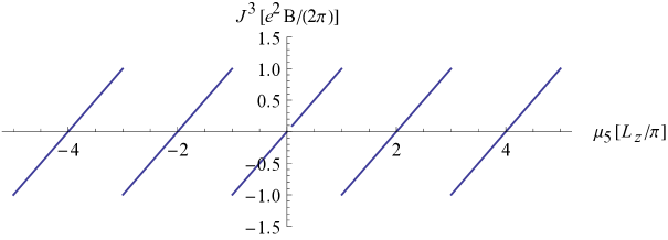
Figure 1: Current density at zero temperature as a function of the chiral chemical potential.

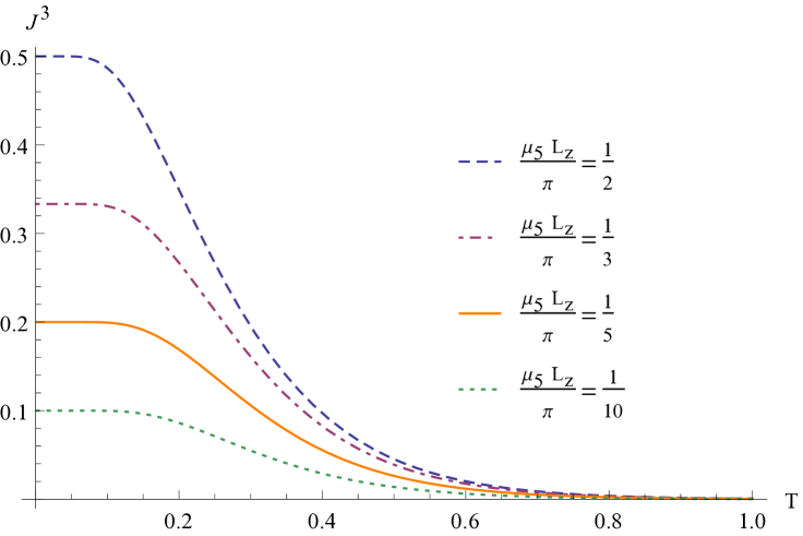
Figure 2: Current density (in units of $\frac{e^{2}B}{2\pi}$) as a function of the temperature (in units of $\frac{L_{z}}{\pi}$), for some values of the axial chemical potential.

IV Conclusions

To summarize, we have performed a full computation of the current associated to the chiral magnetic effect, in the framework of finite temperature field theory, regularized through the gauge-invariant zeta function method in the path integral formulation. From our calculation, some remarkable conclusions arise:

In the first place, there is no CME when the manifold is infinite in the $x^{3}$-direction, which is an evident consequence of gauge invariance, preserved by our regularization method. From our detailed calculations it is evident that any other gauge-invariant regularization will lead to the same conclusion, which is consistent with the results found, for instance, in reference Hou et al. (2011), where canonical quantization was performed, together with a Pauli-Villars regularization, and also in Rebhan et al. (2010), where an holographic approach was employed. Moreover, a generalization of Bloch’s no-go theorem was, indeed, shown to hold for relativistic fields, on the basis of gauge invariance Yamamoto (2015).

On the other hand, we have shown that, in the compact case with antiperiodic boundary conditions, the CME arises from the special modes, whose properties we studied in detail. The associated current coincides, at zero temperature, with the result usually quoted for the non-compact case (see, for instance, Kharzeev (2014)), and seemingly considered to be valid at any temperature in the case of a constant chiral potential. Here, always as a consequence of gauge invariance, this time meaning invariance under “large” gauge transformations, we found that the CME current depends on $\mu_{5}$ in a periodic way. This dependence appears in FIG. 1. We understand this point would be something worth exploring experimentally. As is well known, the zero-temperature expression, combined with the assumption that the chiral potential $\mu_{5}$ is proportional to the four-dimensional anomaly gives, for parallel electric and magnetic fields, a longitudinal magnetic conductance proportional to the square of the magnetic field, something that seems to have been confirmed experimentally by now Kim et al. (2013); Li et al. (2016); Xiong et al. (2015); Li et al. (2015).

Moreover, our calculation shows that, for a given length $L_{z}$, the CME current decreases as the temperature increases. In this article, we have determined its precise dependence on the temperature. In particular, we have reobtained the disappearance of the effect in the noncompact case, by explicitly performing the infinite temperature limit in appendix B. The disappearance of the effect with the temperature is usually attributed to a dependence of the chiral chemical potential with the square of the inverse temperature. We find, instead, that the effect decreases with the temperature, even when $\mu_{5}$ is a constant. Here, we have presented a clear deduction of the way it decreases. The temperature dependence for given values of the remaining variables appears in FIG. 2. We understand that it would also be interesting to contrast this point with experiments.

Now, our explicit calculation leads to some predictions for other boundary conditions, both nonlocal and local ones, in a finite size sample. In the first place, it is easy to see that, in the case of periodic (instead of antiperiodic) nonlocal boundary conditions, the results are essentially the same as in our case, except for a shift in the dependence on $\mu_{5}$. As concerns local elliptic boundary conditions of the bag or even chiral bag type Beneventano et al. (2003), there will not be a CME at all, since such boundary conditions are gauge-invariant. This is in total agreement with previous results as, for instance, the ones obtained in reference Gorbar et al. (2015) for a slab with pure bag boundary conditions. Indeed, in this reference, the CME for a constant chiral chemical potential was shown to vanish, not only in mean but also locally. The same conclusion was arrived to in reference Sitenko (2016), which presents a generalization of the results in Gorbar et al. (2015) to the most general confining local boundary conditions and to finite temperature.

Appendix A Contribution of the special modes to the effective action in the unbounded case

As an example of how gauge invariance prevents the existence of CME at any temperature, we evaluate here the zeta-regularized contribution of the special modes to the effective action and show how, once the gauge invariant zeta regularization is applied, the result is $\alpha$-independent. For these modes,

$$\zeta_{sp}(s) = \left(1+(-1)^{-\frac{s}{2}}\right)\frac{eB}{2\pi}\frac{L_{z}}{2\pi}\rho^{s}\sum_{l=-\infty}^{\infty}\int_{-\infty}^{\infty}dk_{3}\left[\omega_{l}^{2}+\left(k_{3}+\alpha-\mu_{5}\right)^{2}\right]^{-\frac{s}{2}}\,.$$ (36)

In order to perform the analytic extension of $\zeta_{sp}$, we Mellin-transform this last expression, and get

$$\zeta_{sp}(s) = \left(1+(-1)^{-\frac{s}{2}}\right)\frac{eB}{2\pi}\frac{L_{z}}{2\pi}\rho^{s}\sum_{l=-\infty}^{\infty}\int_{-\infty}^{\infty}dk_{3}\frac{1}{\Gamma(s/2)}\int_{0}^{\infty}dt\,t^{\frac{s}{2}-1}e^{-\left[\omega_{l}^{2}+\left(k_{3}+\alpha-\mu_{5}\right)^{2}\right]t}\,,$$ (37)

which, after changing variable to $\kappa=k_{3}+\alpha$, and performing the $\kappa$ integration, leads to

$$\zeta_{sp}(s) = \left(1+(-1)^{-\frac{s}{2}}\right)\frac{eB}{2\pi}\frac{L_{z}}{2\pi}\rho^{s}\sum_{l=-\infty}^{\infty}\frac{\sqrt{\pi}}{\Gamma(s/2)}\int_{0}^{\infty}dt\,t^{\frac{s-1}{2}-1}e^{-\omega_{l}^{2}t}$$ (38)

$$= \left(1+(-1)^{-\frac{s}{2}}\right)\frac{eB}{2\pi}\frac{L_{z}}{2\pi}\rho^{s}\sum_{l=-\infty}^{\infty}\frac{\sqrt{\pi}}{\Gamma(s/2)}\Gamma\left(\frac{s-1}{2}\right)\left((2l+1)\frac{\pi}{\beta}\right)^{1-s}$$

$$= \left(1+(-1)^{-\frac{s}{2}}\right)\frac{eB}{2\pi}\frac{L_{z}}{2\pi}\rho^{s}\frac{s\sqrt{\pi}}{2\Gamma(s/2+1)}\Gamma\left(\frac{s-1}{2}\right)\left(\frac{2\pi}{\beta}\right)^{1-s}2\zeta_{H}(s-1,\frac{1}{2})\,.$$

Now, as can be easily seen, this part of the zeta function vanishes at $s=0$. So, it is easy to perform the $s$-derivative to get this partial contribution to the effective action, which we will call $S_{{\rm eff},sp}$

$$S_{{\rm eff},sp}=-4\pi\frac{eB}{2\pi}\frac{L_{z}}{\beta}\zeta_{H}(-1,\frac{1}{2})\,.$$ (39)

It is clear that, this expression being $\alpha$-independent, gives no contribution whatsoever to a current in the direction of the magnetic field. This lack of CME is a consequence of the gauge invariance of the problem, which is well-known to be preserved by the zeta-function regularization. In fact, $\alpha-\mu_{5}$ can be removed from equation (24) through a gauge transformation.

Appendix B High temperature limit of $J^{3}$

As is well known (see, for instance,Asorey et al. (2013)), in order study the high temperature limit of the CME, i.e. the $\beta\rightarrow 0$-limit of $J^{3}$, we use the inversion formula of the Jacobi Theta function in the index $k$ in (30),

$$\zeta_{sp}(s) = \left(1+(-1)^{-\frac{s}{2}}\right)\frac{eB}{2\pi}\rho^{s}\sum_{l=-\infty}^{\infty}\sum_{k=-\infty}^{\infty}\frac{1}{\Gamma(s/2)}\int_{0}^{\infty}dt\,t^{\frac{s}{2}-1}e^{-\left[\omega_{l}^{2}+\left(q_{k}+\alpha-\mu_{5}\right)^{2}\right]t}$$ (40)

$$= \left(1+(-1)^{-\frac{s}{2}}\right)\frac{eB}{2\pi}\rho^{s}{\left(\frac{2\pi}{L_{z}}\right)}^{-s}\frac{{\pi}^{\frac{1}{2}}}{\Gamma(s/2)}\sum_{l,k=-\infty}^{\infty}\int_{0}^{\infty}dt\,t^{\frac{s-1}{2}-1}(-1)^{k}e^{-\frac{{\pi}^{2}k^{2}}{t}}e^{i\,k(\alpha-\mu_{5})L_{z}}e^{-\left((2l+1)\frac{L_{z}}{2\beta}\right)^{2}t}$$

$$= \left(1+(-1)^{-\frac{s}{2}}\right)\frac{eB}{2\pi}\rho^{s}{\left(\frac{2\pi}{L_{z}}\right)}^{-s}\frac{{\pi}^{\frac{1}{2}}}{\Gamma(s/2)}\left\{\sum_{l=-\infty}^{\infty}\Gamma\left(\frac{s-1}{2}\right)\left[\left((2l+1)\frac{L_{z}}{2\beta}\right)^{2}\right]^{\frac{1-s}{2}}\right.$$

$$+ \left.2\sum_{k=1}^{\infty}\sum_{l=-\infty}^{\infty}\int_{0}^{\infty}dt\,t^{\frac{s-1}{2}-1}(-1)^{k}e^{-\frac{{\pi}^{2}k^{2}}{t}}\cos(k(\alpha-\mu_{5})L_{z})\,e^{-\left((2l+1)\frac{L_{z}}{2\beta}\right)^{2}t}\right\}$$

$$= \left(1+(-1)^{-\frac{s}{2}}\right)\frac{eB}{2\pi}\rho^{s}{\left(\frac{2\pi}{L_{z}}\right)}^{-s}\frac{{\pi}^{\frac{1}{2}}}{\Gamma(s/2)}\left\{2\Gamma\left(\frac{s-1}{2}\right)\left(\frac{L_{z}}{\beta}\right)^{1-s}\zeta_{H}\left(s-1,\frac{1}{2}\right)\right.$$

$$+ \left.8\sum_{k=1}^{\infty}\sum_{l=0}^{\infty}(-1)^{k}\cos(k(\alpha-\mu_{5})L_{z})\left(\frac{2\pi k\beta}{(2l+1)L_{z}}\right)^{\frac{s-1}{2}}K_{\frac{s-1}{2}}\left(\frac{\pi k(2l+1)L_{z}}{\beta}\right)\right\}\,.$$

Performing the $s$-derivative, and evaluating at $s=0$, we obtain an alternative expression for the effective action in equation (33), which allows for the high temperature limit to be taken.

$$S_{{\rm eff},sp}^{k=0}=-4\pi\frac{eB}{2\pi}\frac{L_{z}}{\beta}\zeta_{H}(-1,\frac{1}{2})\,.$$ (41)

This coincides with equation (39), this contribution to $S_{{\rm eff},sp}$ being exactly all that is obtained from the special modes in the unbounded space case. As stated before, it gives no contribution to the current in the direction of the magnetic field.

The $k\neq 0$ terms contribute to $S_{{\rm eff},sp}$ with

$$S_{{\rm eff},sp}^{k\neq 0}=4\frac{eB}{2\pi}\sum_{k=1}^{\infty}\sum_{l=0}^{\infty}\frac{(-1)^{k}}{k}\cos(k(\alpha-\mu_{5})L_{z})\,e^{-\frac{\pi k(2l+1)L_{z}}{\beta}}\,.$$ (42)

Given that, as already explained, the ordinary modes do not give any contribution to the current, all that is left comes from this last equation. We thus obtain an alternative expression for the current $J^{3}$, given by

$$J^{3}=-\frac{2e^{2}B}{\pi\beta}\sum_{k=1}^{\infty}\sum_{l=0}^{\infty}(-1)^{k}L_{z}\sin(k\mu_{5}L_{z})\,e^{-\frac{\pi k(2l+1)L_{z}}{\beta}}\,.$$ (43)

From this expression, it is easily seen that the current in the direction of the magnetic field vanishes in the high temperature limit.

References

- Nielsen and Ninomiya (1983) H. B. Nielsen and M. Ninomiya, Phys. Lett. 130B, 389 (1983).
- Semenoff (1984) G. W. Semenoff, Phys. Rev. Lett. 53, 2449 (1984).
- Haldane (1988) F. D. M. Haldane, Phys. Rev. Lett. 61, 2015 (1988).
- Wehling et al. (2014) T. O. Wehling, A. M. Black-Schaffer, and A. V. Balatsky, Adv. Phys. 63, 1 (2014), arXiv:1405.5774 [cond-mat.mtrl-sci] .
- Gusynin et al. (2007) V. P. Gusynin, S. G. Sharapov, and J. P. Carbotte, Int. J. Mod. Phys. B21, 4611 (2007), arXiv:0706.3016 [cond-mat.mes-hall] .
- Beneventano et al. (2007) C. G. Beneventano, P. Giacconi, E. M. Santangelo, and R. Soldati, J. Phys. A40, F435 (2007), arXiv:hep-th/0701095 [hep-th] .
- Vozmediano et al. (2010) M. A. H. Vozmediano, M. I. Katsnelson, and F. Guinea, Phys. Rept. 496, 109 (2010), arXiv:1003.5179 [cond-mat.mes-hall] .
- Fialkovsky and Vassilevich (2012) I. V. Fialkovsky and D. V. Vassilevich, Proceedings, 10th Conference on Quantum field theory under the influence of external conditions (QFEXT 11): Benasque, Spain, September 18-24, 2011, Int. J. Mod. Phys. A27, 1260007 (2012), [Int. J. Mod. Phys. Conf. Ser.14,88(2012)], arXiv:1111.3017 [hep-th] .
- Cortijo et al. (2012) A. Cortijo, F. Guinea, and M. A. H. Vozmediano, J. Phys. A45, 383001 (2012), arXiv:1112.2054 [cond-mat.mes-hall] .
- Beneventano et al. (2014) C. G. Beneventano, I. V. Fialkovsky, E. M. Santangelo, and D. V. Vassilevich, Eur. Phys. J. B87, 50 (2014), arXiv:1311.0254 [cond-mat.mes-hall] .
- Beneventano et al. (2018) C. G. Beneventano, I. V. Fialkovsky, M. Nieto, and E. M. Santangelo, Phys. Rev. B97, 155406 (2018), arXiv:1803.02760 [cond-mat.mes-hall] .
- Chernodub et al. (2014) M. N. Chernodub, A. Cortijo, A. G. Grushin, K. Landsteiner, and M. A. H. Vozmediano, Phys. Rev. B89, 081407 (2014), arXiv:1311.0878 [hep-th] .
- Witten (2016) E. Witten, Riv. Nuovo Cim. 39, 313 (2016), arXiv:1510.07698 [cond-mat.mes-hall] .
- Pozo et al. (2018) O. Pozo, Y. Ferreiros, and M. A. H. Vozmediano, Phys. Rev. B98, 115122 (2018), arXiv:1802.02632 [cond-mat.str-el] .
- Fukushima et al. (2008) K. Fukushima, D. E. Kharzeev, and H. J. Warringa, Phys. Rev. D78, 074033 (2008), arXiv:0808.3382 [hep-ph] .
- Kharzeev (2014) D. E. Kharzeev, Prog. Part. Nucl. Phys. 75, 133 (2014), arXiv:1312.3348 [hep-ph] .
- Landsteiner (2016) K. Landsteiner, Proceedings, 56th Cracow School of Theoretical Physics : A Panorama of Holography: Zakopane, Poland, May 24-June 1, 2016, Acta Phys. Polon. B47, 2617 (2016), arXiv:1610.04413 [hep-th] .
- Adler (1969) S. L. Adler, Phys. Rev. 177, 2426 (1969).
- Bell and Jackiw (1969) J. S. Bell and R. Jackiw, Nuovo Cim. A60, 47 (1969).
- Kim et al. (2013) H.-J. Kim, K.-S. Kim, J. F. Wang, M. Sasaki, N. Satoh, A. Ohnishi, M. Kitaura, M. Yang, and L. Li, Phys. Rev. Lett. 111, 246603 (2013), arXiv:1307.6990 [cond-mat.str-el] .
- Li et al. (2016) Q. Li, D. E. Kharzeev, C. Zhang, Y. Huang, I. Pletikosic, A. V. Fedorov, R. D. Zhong, J. A. Schneeloch, G. D. Gu, and T. Valla, Nature Phys. 12, 550 (2016), arXiv:1412.6543 [cond-mat.str-el] .
- Xiong et al. (2015) J. Xiong, S. K. Kushwaha, T. Liang, J. W. Krizan, M. Hirschberger, W. Wang, R. J. Cava, and N. P. Ong, Science 350, 413 (2015).
- Li et al. (2015) C.-Z. Li, L.-X. Wang, H. Liu, J. Wang, Z.-M. Liao, and D.-P. Yu, Nature Communications 6, 10137 (2015).
- Dowker and Critchley (1976) J. S. Dowker and R. Critchley, Phys. Rev. D13, 3224 (1976).
- Valgushev et al. (2016) S. N. Valgushev, M. Puhr, and P. V. Buividovich, Proceedings, 33rd International Symposium on Lattice Field Theory (Lattice 2015): Kobe, Japan, July 14-18, 2015, PoS LATTICE2015, 043 (2016), arXiv:1512.01405 [cond-mat.str-el] .
- Yamamoto (2015) N. Yamamoto, Phys. Rev. D 92, 085011 (2015).
- Dunne (1999) G. V. Dunne, “Aspects of chern-simons theory,” (1999), arXiv:hep-th/9902115 [hep-th] .
- Gilkey and Kirsten (2005) P. Gilkey and K. Kirsten, Lett. Math. Phys. 73, 147 (2005), arXiv:math/0510152 [math-ap] .
- Beneventano et al. (2003) C. G. Beneventano, P. B. Gilkey, K. Kirsten, and E. M. Santangelo, J. Phys. A36, 11533 (2003), arXiv:hep-th/0306156 [hep-th] .
- Fialkovsky et al. (2019) I. Fialkovsky, M. Kurkov, and D. Vassilevich, Physical Review D 100 (2019), 10.1103/physrevd.100.045026.
- Gorbar et al. (2015) E. V. Gorbar, V. A. Miransky, I. A. Shovkovy, and P. O. Sukhachov, Physical Review B 92 (2015), 10.1103/physrevb.92.245440.
- Sitenko (2016) Y. A. Sitenko, Phys. Rev. D 94, 085014 (2016).
- Basar and Dunne (2013) G. Basar and G. V. Dunne, Lect. Notes Phys. 871, 261 (2013), arXiv:1207.4199 [hep-th] .
- Gradshteyn and Ryzhik (2014) I. Gradshteyn and I. Ryzhik, Table of Integrals, Series, and Products (Elsevier, 2014).
- Gamboa Saravi et al. (1981) R. E. Gamboa Saravi, F. A. Schaposnik, and J. E. Solomin, Nucl. Phys. B185, 239 (1981).
- Sissakian et al. (1998) A. N. Sissakian, O. Y. Shevchenko, and S. B. Solganik, “Topological effects in medium,” (1998), arXiv:hep-th/9806047 [hep-th] .
- Hou et al. (2011) D.-f. Hou, H. Liu, and H.-c. Ren, Journal of High Energy Physics 2011 (2011), 10.1007/jhep05(2011)046.
- Rebhan et al. (2010) A. Rebhan, A. Schmitt, and S. A. Stricker, Journal of High Energy Physics 2010 (2010), 10.1007/jhep01(2010)026.
- Asorey et al. (2013) M. Asorey, C. G. Beneventano, D. D’Ascanio, and E. M. Santangelo, JHEP 04, 068 (2013), arXiv:1212.6220 [hep-th] .