Capacity, Bandwidth, and Compositionality in Emergent Language Learning

Abstract.

Many recent works have discussed the propensity, or lack thereof, for emergent languages to exhibit properties of natural languages. A favorite in the literature is learning compositionality. We note that most of those works have focused on communicative bandwidth as being of primary importance. While important, it is not the only contributing factor. In this paper, we investigate the learning biases that affect the efficacy and compositionality in multi-agent communication. Our foremost contribution is to explore how the capacity of a neural network impacts its ability to learn a compositional language. We additionally introduce a set of evaluation metrics with which we analyze the learned languages. Our hypothesis is that there should be a specific range of model capacity and channel bandwidth that induces compositional structure in the resulting language and consequently encourages systematic generalization. While we empirically see evidence for the bottom of this range, we curiously do not find evidence for the top part of the range and believe that this is an open question for the community.

1. Introduction

Compositional language learning in the context of multi agent emergent communication has been extensively studied (Sukhbaatar et al., 2016; Foerster et al., 2016; Lazaridou et al., 2017; Baroni, 2020). These works have found that while most emergent languages do not tend to be compositional, they can be guided towards this attribute through artificial task-specific constraints (Kottur et al., 2017; Lee et al., 2018).

In this paper, we focus on how a neural network, specifically a generative one, can learn a compositional language. Moreover, we ask how this can occur without task-specific constraints. To accomplish this, we first define what is a language and what we mean by compositionality. In tandem, we introduce precision and recall, two metrics that help us measure how well a generative model at large has learned a grammar from a finite set of training instances. We then use a variational autoencoder with a discrete sequence bottleneck to investigate how well the model learns a compositional language, in addition to what affects that learning. This allows us to derive residual entropy, a third metric that reliably measures compositionality in our particular environment. We use this metric to cross-validate precision and recall. Finally, while there may be a connection between our study and human-level languages, we do not experiment with human data or languages in this work.

Our environment lets us experiment with a syntactic, compositional language while varying the channel width and the number of parameters, our surrogate for the capacity of a model. Our experiments reveal that our smallest models are only able to solve the task when the channel is wide enough to allow for a surface-level compositional representation. In contrast, large models learn a language as long as the channel is large enough. However, large models also have the ability to memorize the training set. We hypothesize that this memorization would lead to non-compositional representations and overfitting, albeit this does not yet manifest empirically. This setup allows us to test our hypothesis that there is a network capacity above which models will tend to produce languages with non-compositional structure.

2. Related Work

There has recently been renewed interest in studies of emergent language (Foerster et al., 2016; Lazaridou et al., 2017; Havrylov and Titov, 2017) that originated with works such as Steels and Kaplan (2000); Steels (1997). Some of these approaches use referential games (Evtimova et al., 2018; Lazaridou et al., 2018; Lowe* et al., 2020) to produce an emergent language that ideally has properties of human languages, with compositionality being a commonly sought after property (Barrett et al., 2018; Baroni, 2020; Chaabouni et al., 2019a).

Our paper is most similar to Kottur et al. (2017), which showed that compositional language arose only when certain constraints on the agents are satisfied. While the constraints they examined were either making their models memoryless or having a minimal vocabulary in the language, we hypothesized about the importance for agents to have small capacity relative to the number of disentangled representations (concepts) to which they are exposed. This is more general because both of the scenarios they described fall under the umbrella of reducing model capacity. To ask this, we built a much bigger dataset to illuminate how capacity and channel width effect the resulting compositionality in the language. LiskaLiska et al. (2018) suggests that the average training run for recurrent neural networks does not converge to a compositional solution, but that a large random search will produce compositional solutions. This implies that the optimization approach biases learning, which is also confirmed in our experiments. However, we further analyze other biases. SpikeSpike et al. (2017) describes three properties that bias models towards successful learned signaling: the creation and transmission of referential information, a bias against ambiguity, and information loss. This lies on a similar spectrum to our work, but pursues a different intent in that they study biases that lead to optimal signaling; we seek compositionality. Each of Verhoef et al. (2016); Kirby et al. (2015); Zaslavsky et al. (2018) examine the trade-off between expression and compression in both emergent and natural languages, in addition to how that trade-off affects the learners. We differ in that we target a specific aspect of the agent (capacity) and ask how that aspect biases the learning. ChenChen et al. (2018) describes how the probability distribution on the set of all strings produced by a recurrent model can be interpreted as a weighted language; this is relevant to our formulation of the language.

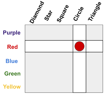
Figure 1. The grid above shows five shapes and five colors. Agents with a non-compositional language can use this shared map to communicate ”Red Circle” with only $\lceil\log_{2}{5^{2}}\rceil=5$ bits. If they instead used a compositional language, it would require $\lceil\log_{2}5\rceil=3$ bits for each concept for a total of $6$ bits to convey the string. On the other hand, the agent needs $25$ memory slots to store the concepts in the former case but only $10$ slots in the compositional case. This trade-off exemplifies the motivation for our investigation because it suggests that a key driver of compositionality in language is the capacity of an agent relative to the total number of objects in its environment.

Most other works studying compositionality in emergent languages (Andreas, 2019; Mordatch and Abbeel, 2018; Chaabouni et al., 2019b; Lee et al., 2019) have focused on learning interpretable representations. See Hupkes et al. (2020) for a broad survey of the different approaches. By and large, these are orthogonal to our work because none pose the question we ask - how does an agent’s capacity effect the resulting language’s compositionality?

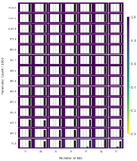
(a) Precision

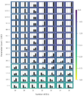
(b) Recall

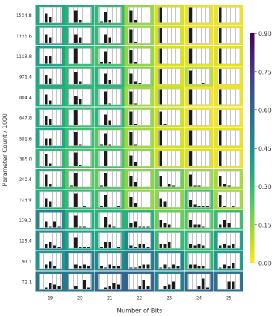
(c) Entropy

Figure 2. Histograms for model A showing precision, recall (defined in § 3.2), and entropy (defined in § 5.1) over the test set. We show results for bits $19$ to $25$ and parameter range $72k$ to $1534k$ (details in § 5). Each bit/parameter combination is trained for $10$ seeds over $200k$ steps. Precision and Recall are as described in Eqs. (5) and (6) with $M=|D_{\text{test}}|$ and $N=10000$.

3. Compositional Language and Learning

We start by defining a language and what it means for a language to be compositional. We then discuss what it means for a network to learn a compositional language, based on which we derive evaluation metrics.

3.1. Compositional Language

A language $L$ is a subset of $\Sigma^{*}$, where $\Sigma$ denotes an alphabet and $s$ denotes a string:

$$\Sigma^{*}=\left\{s\mid\forall i=1,\ldots,|s|\quad s_{i}\in\Sigma\wedge|s|\geq 0\right\}.$$

In this paper, we constrain a language to contain only finite-length strings, i.e., $|s|<\infty$, implying that $L$ is a finite language. We use $K_{\max}$ to denote the maximum length of any $s\in L$.

We define a generator $G$ from which we can sample one valid string $s\in L$ at a time. It never generates an invalid string and generates all the valid strings in $L$ in finite time such that

$$s\sim G\Leftrightarrow s\in L.$$ (1)

We define the length $|G|$ of the description of $G$ as the sum of the number of non-terminal symbols $\mathcal{N}$ and the number of production rules $\mathcal{P}$, where $|\mathcal{N}|<\infty$ and $|\mathcal{P}|<\infty$. Each production rule $\rho\in\mathcal{P}$ takes as input an intermediate string $s^{\prime}\in(\Sigma\cup\mathcal{N})^{*}$ and outputs another string $s^{\prime\prime}\in(\Sigma\cup\mathcal{N})^{*}$. The generator starts from an empty string $\varnothing$ and applies an applicable production rule (uniformly selected at random) until the output string consists only of characters from the alphabet (terminal symbols).

Languages and compositionality

When the number of such production rules $|\mathcal{P}|$ plus the number of intermediate symbols $|\mathcal{N}|$ is smaller than the size $|L|$ of the language that $G$ generates, we call $L$ a compositional language. In other words, $L$ is compositional if and only if $|L|>|\mathcal{P}|+|\mathcal{N}|$.

One such example is when we have sixty characters in the alphabet, $\Sigma=\left\{0,1,2,\ldots,59\right\}$, and six intermediate symbols, $\mathcal{N}=\left\{C_{1},C_{2},\ldots,C_{6}\right\}$, for a total of $6\times 10+1$ production rules $\mathcal{P}$:

• $\varnothing\to C_{1}C_{2}C_{3}C_{4}C_{5}C_{6}$.

• For each $i\in[1,6]$, $C_{i}\to w$, where $w\in\left\{10i-10,\ldots,10i-1\right\}$

From these production rules and intermediate symbols, we obtain a language of size $10^{6}\gg 67=|\mathcal{P}|+|\mathcal{N}|$. We thus consider this language to be compositional and will use it in our experiments.

3.2. Learning a language

We consider the problem of learning an underlying language $L^{\star}$ from a finite set of training strings randomly drawn from it:

$$D=\left\{s|s\sim G^{\star}\right\}$$

where $G^{\star}$ is the minimal length generator associated with $L^{\star}$. We assume $|D|\ll|L^{\star}|$ and our goal is to use $D$ to learn a language $L$ that approximates $L^{\star}$ as well as possible. We know that there exists an equivalent generator $G$ for $L$, and so our problem becomes estimating a generator from this finite set rather than reconstructing an entire set of strings belonging to the original language $L^{*}$.

We cast the problem of estimating a generator $G$ as density modeling, in which case the goal is to estimate a distribution $p(s)$. Sampling from $p(s)$ is equivalent to generating a string from the generator $G$. Language learning is then

$$\max_{p\in\mathcal{M}}\frac{1}{|D|}\sum_{n=1}^{|D|}\log p(s_{n})+\lambda R(p),$$ (2)

where $R$ is a regularization term, $\lambda$ its strength, and $\mathcal{M}$ is a model space.

Evaluation metrics

When the language was learned perfectly, any string sampled from the learned distribution $p(s)$ must belong to $L^{\star}$. Also, any string in $L^{\star}$ must be assigned a non-zero probability under $p(s)$. Otherwise, the set of strings generated from this generator, implicitly defined via $p(s)$, is not identical to the original language $L^{\star}$. This observation leads to two metrics for evaluating the quality of the estimated language with the distribution $p(s)$, precision and recall:

$$\text{Precision}(L^{\star},p)=\frac{1}{|L^{\star}|}\sum_{s\in L}\mathbb{I}(s\in L^{\star})$$ (3)

$$\text{Recall}(L^{\star},p)=\sum_{s\in L^{\star}}\log p(s)$$ (4)

where $\mathbb{I}(x)$ is the indicator function. These metrics are designed to be fit for any compositional structure rather than one-off evaluation approaches. Because these are often intractable to compute, we approximate them using Monte-Carlo by sampling $N$ samples from $p(s)$ for calculating precision and $M$ uniform samples from $L^{\star}$ for calculating recall.

$$\text{Precision}(L^{\star},p)\approx\frac{1}{N}\sum_{n=1}^{N}\mathbb{I}(s_{n}\in L^{\star})$$ (5)

$$\text{Recall}(L^{\star},p)\approx\sum_{m=1}^{M}\log p(s_{m}),$$ (6)

where $s_{n}\sim p(s)$ and $s_{m}$ is a uniform sample from $L^{\star}$.

3.3. Compositionality, learning, and capacity

When learning an underlying compositional language $L^{\star}$, there are three possible outcomes:

Overfitting: $p(s)$ could memorize all the strings that were presented when solving Eq. (2) and assign non-zero probabilities to those strings and zero probabilities to all others. This would maximize precision, but recall will be low as the estimated generator does not cover $L^{\star}$.

Systematic generalization: $p(s)$ could capture the underlying compositional structures of $L^{\star}$ characterized by the production rules $\mathcal{P}$ and intermediate symbols $\mathcal{N}$. In this case, $p(s)$ will assign non-zero probabilities to all the strings that are reachable via these production rules (and zero probability to all others) and generalize to strings from $L^{\star}$ that were unseen during training, leading to high precision and recall. This behavior was characterized in Lake (2019).

Failure: $p(s)$ may neither memorize the entire training set nor capture the underlying production rules and intermediate symbols, resulting in both low precision and recall.

We hypothesize that a major factor determining the compositionality of the resulting language is the capacity of the most complicated distribution $p(s)$ within the model space $\mathcal{M}$. When the model capacity is too high, the first case of total memorization is likely. When it is too low, the third case of catastrophic failure will happen. Only when the model capacity is just right will language learning correctly capture the compositional structure underlying the original language $L^{\star}$ and exhibit systematic generalization (Bahdanau et al., 2019). We empirically investigate this hypothesis using a neural network as a language learner, in particular a variational autoencoder with a discrete sequence bottleneck. This admits the interpretation of a two-player ReferIt game (Lewis, 1969) in addition to being a density estimator of $p(s)$. Together, these let us use recall and precision to analyze the resulting emergent language.

4. Variational autoencoders and their capacity

A variational autoencoder (Kingma and Welling, 2014) consists of two neural networks which are often referred to as an encoder $f_{\theta}$, a decoder $g_{\phi}$, and a prior $p_{\lambda}$. These two networks are jointly updated to maximize the variational lower bound to the marginal log-probability of training instances $s$:

$$\mathcal{L}(\theta,\phi,\lambda;s)=\mathbb{E}_{z\sim f_{\theta}(z|s)}\left[\log g_{\phi}(s|z)\right]-\text{KL}(f_{\theta}(z|s)\|p_{\lambda}).$$ (7)

We use $\mathcal{L}$ as a proxy to the true $p(s)$ captured by this model. Once trained, we can efficiently sample $\tilde{z}$ from the prior $p_{\lambda}$ and then sample a string from $g_{\phi}(s|\tilde{z})$.

The usual formulation of variational autoencoders uses a continuous latent variable $z$, which conveniently admits reparametrization that reduces the variance in the gradient estimate. However, this infinitely large latent variable space makes it difficult to understand the resulting capacity of the model. We thus constrain the latent variable to be a binary string of a fixed length $l$, i.e., $z\in\left\{0,1\right\}^{l}$. Assuming deterministic decoding, i.e., $\operatorname*{argmax}_{s}\log g_{\phi}(s|z)$, this puts a strict upperbound of $2^{l}$ on the size of the language $|L|$ captured by the variational autoencoder.

4.1. Variational autoencoder as a communication channel

As described above, using variational autoencoders with a discrete sequence bottleneck allows us to analyze the capacity of the model in terms of computation and bandwidth. We can now interpret this variational autoencoder as a communication channel in which a novel protocol must emerge as a by-product of learning. We will refer to the encoder as the speaker and the decoder as the listener when deployed in this communication game. If each string $s\in L^{\star}$ in the original language is a description of underlying concepts, then the goal of the speaker $f_{\theta}$ is to encode those concepts in a binary string $z$ following an emergent communication protocol. The listener $g_{\phi}$ receives this string and must interpret which set of concepts were originally seen by the speaker.

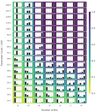
(a) Model A Training

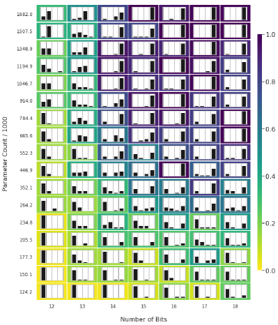
(b) Model A Testing

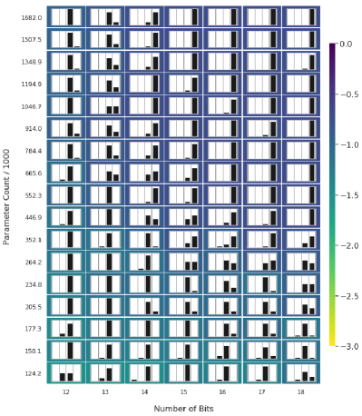
(c) Model A Recall

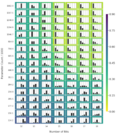
(d) Model A Entropy

Figure 3. Results when running Model A with $N=4$ categories instead of $N=6$. We show results for bits $12$ to $18$ and parameter range $124k$ to $1682k$. We need at least $\lceil\log_{2}10^{4}\rceil=14$ bits to cover all the input combinations. Observe that there is not much difference to the $N=6$ scenario show in fig 2. See § 3.2 and §5.1 for the definitions of recall and entropy.

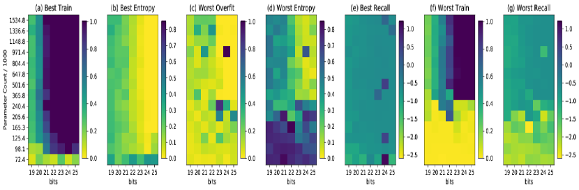
Figure 4. Main results for model A showing best and worst performances of the proposed metrics over $10$ seeds. See Section 5.2 for detailed analysis. Panels (a) and (f) show the accuracy of the training data, (b) and (d) show entropy, (e) and (g) show recall over the test data, and (c) plots the max difference in accuracy between training and test.

Our setup

We simplify and assume that each of the characters in the string $s\in L^{\star}$ correspond to underlying concepts. While the inputs are ordered according to the sequential concepts, our model encodes them using a bag of words (BoW) representation.

The speaker $f_{\theta}$ is parameterized using a recurrent policy which receives the sequence of concatenated one-hot input tokens of $s$ and converts each of them to an embedding. It then runs an LSTM (Hochreiter and Schmidhuber, 1997) non-autoregressively for $l$ timesteps taking the flattened representation of the input embeddings as its input and linearly projecting each result to a probability distribution over $\{0,1\}$. This results in a sequential Bernoulli distribution over $l$ latent variables:

$$f_{\theta}(z|s)=\prod_{t=1}^{l}p(z_{t}|s;\theta)$$

From this distribution, we can sample a latent string $z=(z_{1},\ldots,z_{l})$.

The listener $g_{\phi}$ receives $z$ and uses a BoW representation to encode them into its own embedding space. Taking the flattened representation of these embeddings as input, we run an LSTM for $|\mathcal{N}|$ time steps, each time outputting a probability distribution over the full alphabet $\Sigma$:

$$g_{\phi}(s|z)=\prod_{j=1}^{|\mathcal{N}|}p(s_{j}|z;\phi)$$

To train the whole system end-to-end (Sukhbaatar et al., 2016; Mordatch and Abbeel, 2018) via backpropogation, we apply a continuous approximation to $z_{t}$ that depends on a learned temperature parameter $\tau$. We use the ‘straight-through‘ version of Gumbel-Softmax (Jang et al., 2017; Maddison et al., 2017) to convert the continuous distribution to a discrete distribution for each $z_{t}$. This corresponds to the original discrete distribution in the zero-temperature limit. The final sequence of one hot vectors encoding $z$ is our message, which is passed to the listener $g_{\phi}$. If $G_{j}\sim\textrm{Gumbel}(0,1)$ and the Bernoulli random variable corresponding to $z_{t}$ has class probabilities $z_{t_{0}}$ and $z_{t_{1}}$, then $z_{t}=\texttt{one\_hot}(\underset{j}{\arg\max}[G_{j}+\log z_{t_{j}}])$.

The prior $p_{\lambda}$ encodes the message $z$ using a BoW representation. It gives the probability of $z$ according to the prior (binary) distribution for each $z_{t}$ and is defined as:

$$p_{\lambda}(z)=\prod_{t=1}^{l}p(z_{t}|\lambda).$$

This can be used both to compute the prior probability of a latent string and also to efficiently sample from $p_{\lambda}$ using ancestral sampling. Penalizing the KL divergence between the speaker’s distribution and the prior distribution in Eq. (7) encourages the emergent protocol to use latent strings that are as diverse as possible.

4.2. Capacity of a variational autoencoder with discrete sequence bottleneck

This view of a variational autoencoder with discrete sequence bottleneck presents an opportunity for us to separate the model’s capacity into two parts. The first part is the capacity of the communication channel, imposed by the size of the latent variable. As described earlier, the size of the original language $L^{\star}$ that can be perfectly captured by this model is strictly upper bounded by $2^{l}$, where $l$ is the preset length of the latent string $z$. If $l<\log_{2}|L^{\star}|$, the model will not be able to learn the language completely, although it may memorize all the training strings $s\in D$ if $l\geq\log_{2}|D|$. A resulting question is whether $2^{l}\geq|L^{\star}|$ is a sufficient condition for the model to learn $L^{\star}$ from a finite set of training strings.

The second part involves the capacity of the speaker and listener to map between the latent variable $z$ and a string $s$ in the original language $L^{\star}$. Taking the parameter count as a proxy to the number of patterns that could be memorized by a neural network, we can argue that the problem can be solved if the speaker and listener each have $\Omega(l|L^{\star}|)$ parameters, in which case they can implement a hashmap between a string in the original language $L^{\star}$ and that of the learned latent language defined by the $z$ strings.

However, when the underlying language is compositional as defined in §3.1, we can have a much more compact representation of the entire language than a hashmap. Given the status quo understanding of neural networks, it is impossible to correlate the parameter count with the language specification (production rules and intermediate symbols) and the complexity of using that language. It is however reasonable to assume that there is a monotonic relationship between the number of parameters $|\theta|$, or $|\phi|$, and the capacity of the network to encode the compositional structures underlying the original language (Collins et al., 2017). Thus, we use the parameter count as a proxy to measure the capacity.

In summary, there are two axes in determining the capacity of the proposed model: the length of the latent sequence $l$ and the number of parameters $|\theta|$ ($|\phi|$) in the speaker (listener). We vary these two quantities in the experiments and investigate how they affect compositional language learning by the model.

4.3. Implications and hypotheses on compositionality

Under this framework for language learning, we can make the following observations:

• If the length of the latent sequence $l<\log_{2}|L^{\star}|$, it is impossible for the model to avoid the failure case because there will be $|L^{\star}|-2^{l}$ strings in $L^{\star}$ that cannot be generated from the trained model. Consequently, recall cannot be maximized. However, this may be difficult to check using the sample-based estimate as the chance of sampling $s\in L^{\star}\backslash\int g_{\phi}(s|z)p_{\lambda}(z)\text{d}z$ decreases proportionally to the size of $L^{\star}$. This is especially true when the gap $|L^{\star}|-2^{l}$ is narrow.

• When $l\geq\log_{2}|L^{\star}|$, there are three cases. The first is when there are not enough parameters $\theta$ to learn the underlying compositional grammar given by $\mathcal{P}$, $\mathcal{N}$, and $\Sigma$, in which case $L^{\star}$ cannot be learned. The second case is when the number of parameters $|\theta|$ is greater than that required to store all the training strings, i.e., $|\theta|=O(l|D|)$. Here, it is highly likely for the model to overfit as it can map each training string with a unique latent string without having to learn any of $L^{\star}$’s compositional structure. Lastly, when the number of parameters lies in between these two poles, we hypothesize that the model will capture the underlying compositional structure and exhibit systematic generalization.

In short, we hypothesize that the effectiveness of compositional language learning is maximized when both the length of the latent sequence is large enough ($l\geq\log|L^{\star}|$), and the number of parameters $|\theta|$ is between $k(|\mathcal{P}|+|\mathcal{N}|+|\Sigma|)$ and $kl|D|$ for some positive integer $k$. Our experiments test this by varying the length of the latent sequence $l$ and the number of parameters $|\theta|$ while checking the sample-based estimates of precision and recall (Eq. (5)–(6)).

5. Experiments

Data

	Model A	Model B
speaker Total	708k	670k
listener Total	825k	690k
speaker Embedding	100	40
speaker LSTM	200	300
speaker Linear	300	60
listener Embedding	300	125
listener LSTM	300	325

Table 1. The base hyperparameter counts used in our experiments for each of models A and B.

As described in §3.1, we run experiments where the size of the language is much larger than the number of production rules. The task is to communicate $6$ concepts, each of which have $10$ possible values with a total dataset size of $10^{6}$. We build three finite datasets $D_{\text{train}}$, $D_{\text{val}}$, $D_{\text{test}}$:

$$S_{\text{train}}=\left\{s\in L^{\star}\mid s\neq(*C^{\text{val}}_{1}*C^{\text{val}}_{2}*)\wedge s\neq(*C^{\text{test}}_{1}*C^{\text{test}}_{2}*)\right\}$$

$$S_{\text{val}}=\left\{s=(*C^{\text{val}}_{1}*C^{\text{val}}_{2}*)\right\}$$

$$S_{\text{test}}=\left\{s=(*C^{\text{test}}_{1}*C^{\text{test}}_{2}*)\wedge s\notin D_{\text{val}}\right\}$$

$$D_{\text{train}}=\text{subsample}\left(S_{\text{train}},N_{\text{train}}\right)$$

$$D_{\text{val}}=\text{subsample}\left(S_{\text{val}},N_{\text{val}}\right)$$

$$D_{\text{test}}=\text{subsample}\left(S_{\text{test}},N_{\text{val}}\right),$$

where $\text{subsample}(S,N)$ uniformly selects $N$ random items from $S$ without replacement. The randomly selected concept values $(C^{\text{val}}_{1},C^{\text{val}}_{2})$ and $(C^{\text{test}}_{1},C^{\text{test}}_{2})$ ensure that concept combinations are unique to each set. The $*$ symbol refers to any number of concepts, as in regular expressions.

Models and Learning

We train the proposed variational autoencoder (described in §4.1) on $D_{\text{train}}$, using the Adam optimizer (Kingma and Ba, 2015) with a learning rate of $3\times 10^{-3}$, weight decay coefficient of $10^{-4}$ and a batch size of $1000$. The Gumbel-Softmax temperature parameter $\tau$ in is initialized to 1. Since systematic generalization may only happen in some training runs (Weber et al., 2018), each model is trained for each of $10$ seeds over $200k$ steps. We trained our models using (Paszke et al., 2019).

We train two sets of models. Each set is built from an independent base model, the architectures of which are described in Table 1. We gradually decrease the number of LSTM units from the base model by a factor $\alpha\in\left(0,1\right]$. This is how we control the number of parameters ($|\theta|$ and $|\phi|$), a factor we hypothesize to influence the resulting compositionality. We obtain seven models from each of these by varying the length of the latent sequence $l$ from $\left\{19,20,21,22,23,24,25\right\}$. These were chosen because we both wanted to show a range of bits and because we need at least $20$ bits to cover the $10^{6}$ strings in $L^{*}$ ($\lceil\log_{2}10^{6}\rceil=20$).

Note that results for the two models are similar and so we arbitrarily spotlight one of them - model A. We additionally show the results for model B in Figs. 5, 6, and 8, but do not dive into its results in the main section.

5.1. Evaluation: Residual Entropy

Our setup allows us to design a metric by which we can check the compositionality of the learned language $L$ by examining how the underlying concepts are described by a string. For instance, $(2,11,24,31,44,56)\in L^{\star}$ describes that $C_{1}=2$, $C_{2}=11$, $C_{3}=24$, $C_{4}=31$, $C_{5}=44$ and $C_{6}=56$. Furthermore, we know that the value of a concept $C_{i}$ is independent of the other concepts $C_{j\neq i}$, and so our custom generative setup with a discrete latent sequence allows us to inspect a learned language $L$ by considering $z$.

Let $p$ be a sequence of partitions of $\left\{1,2,\ldots,l\right\}$. We define the degree of compositionality as the ratio between the variability of each concept $C_{i}$ and the variability explained by a latent subsequence $z[p_{i}]$ indexed by an associated partition $p_{i}$. More formally, the degree of compositionality given the partition sequence $p$ is defined as a residual entropy

$$\text{re}(p,L,L^{\star})=\frac{1}{|\mathcal{N}|}\sum_{i=1}^{|\mathcal{N}|}\mathcal{H}_{L}(C_{i}|z[p_{i}])/\mathcal{H}_{L^{\star}}(C_{i})$$

where there are $|\mathcal{N}|$ concepts by the definition of our language. When each term inside the summation is close to zero, it implies that a subsequence $z[p_{i}]$ explains most of the variability of the specific concept $C_{i}$, and we consider this situation compositional. The residual entropy of a trained model is then the smallest $\text{re}(p)$ over all possible sequences of partitions $\mathcal{P}$ and spans from $0$ (compositional) to $1$ (non-compositional).

$$\text{re}(L,L^{\star})=\min_{p\in\mathcal{P}}\text{re}(p,L,L^{\star}).$$

5.2. Results

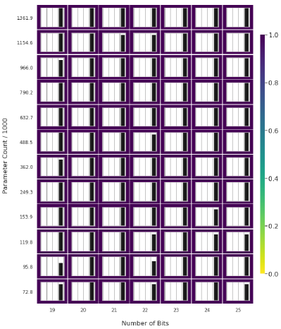
(a) Model B Precision

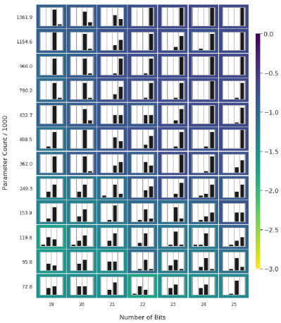
(b) Model B Recall

Figure 5. Precision and recall for model B. Like model A, model B has perfect precision. However, its recall chart shows a different story. The first takeaway is that while there is still a strong region in the top right bounded below by $\sim 360k$ parameters, it does not extend to $22$ bits on the left side. This supports our notion of a minimal capacity threshold but adds a wrinkle in that this architecture influences the model’s ability to succeed with fewer bits.

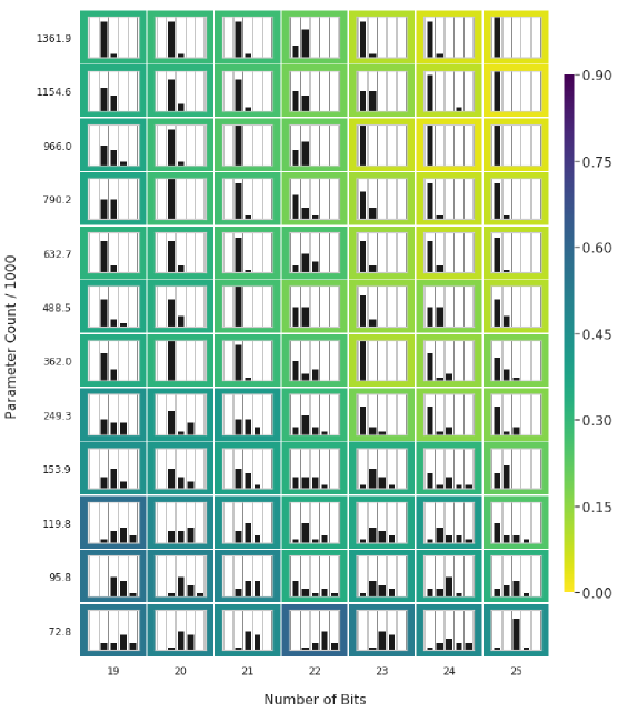
Figure 6. Entropy metric for model B as described in §5.1. Similar to model A, we see that model B’s entropy supports the view we had of its recall in Figure 5 - there is a strong region in the top right that supports the notion of a minimal capacity and bit threshold.

Fig. 4 shows the main findings of our research. In plot (a), we see the parameter counts at the threshold. Below these values, the model cannot solve the task but above these, it can solve it. Further, observe the curve delineated by the lower left corner of the shift from unsuccessful to successful models. This inverse relationship between bits and parameters shows that the more parameters in the model, the fewer bits it needs to solve the task. Note however that it could only solve the task with fewer bits if it was forming a non-compositional code, suggesting that higher parameter models are able to do so while lower parameter ones cannot.

Observe further that all of our models above the minimum threshold (72,400) have the capacity to learn a compositional code. This is shown by the perfect training accuracy achieved by all of those models in plot (a) for 24 bits and by the perfect compositionality (zero entropy) in plot (b) for 24 bits. Together with the above, this validates that learning compositional codes requires less capacity than learning non-compositional codes.

Plot (c) confirms our hypothesis that large models can memorize the entire dataset. The 24 bit model with 971,400 parameters achieves a train accuracy of 1.0 and a validation accuracy of 0.0. Cross-validating this with plots (d) and (g), we find that a member of the same parameter class is non-compositional and that there is one that achieves unusually low recall. We verified that these are all the same seed, which shows that the agents in this model are memorizing the dataset. This is supplemented by Fig. 7 where we see the non-compositional behavior by plotting residual entropy versus overfitting.

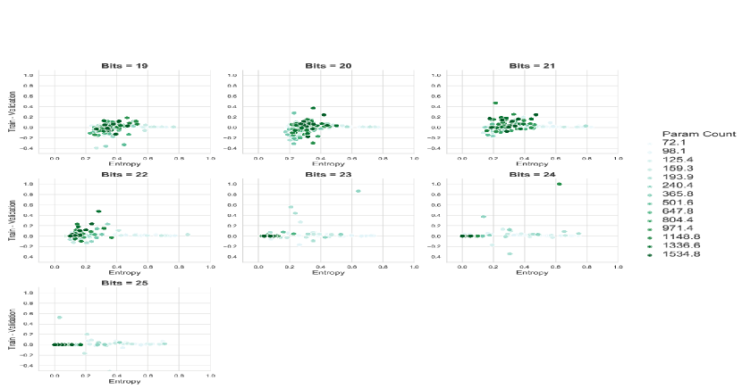
Figure 7. Model A Entropy vs Overfitting: Charts showing per-bit results for Entropy vs (Train - Validation) over the parameter range. Observe the two models in bits $23$ and $24$ which were too successful in producing a non-compositional code and consequently overfit to the data.

Plots (b) and (e) show that our compositionality metrics pass two sanity checks - high recall and perfect entropy can only be achieved with a channel that is sufficiently large (i.e. 24 bits) to allow for a compositional latent representation.

Plot (f) shows that while the capacity does not affect the ability to learn a compositional language across the model range, it does change the learnability. Here we find that smaller models can fail to solve the task for any bandwidth, which coincides with literature suggesting a link between overparameterization and learnability (Li and Liang, 2018; Du et al., 2019). This is supported by the efficacy results in Fig. 8.

Finally, as expected, we find that no model learns to solve the task with $<20$ bits, validating that the minimum required number of bits for learning a language of size $|L|$ is $\lceil\log(|L|)\rceil$. We also see that no model learns to solve it for $20$ bits, which is likely due to optimization difficulties.

In Fig. 2, we present histograms showing precision, recall and residual entropy measured for each bit and parameter combination over the test set. The histograms show the distributions of these metrics, upon which we make a number of observations.

We first confirm the effectiveness of training by observing that almost all the models achieve perfect precision (Fig. 2 (a)), implying that $L\subseteq L^{\star}$, where $L$ is the language learned by the model. This occurs even with our learning objective in Eq. (7) encouraging the model to capture all training strings rather than to focus on only a few training strings.

A natural follow-up question is how large is $L^{\star}\backslash L$. We measure this with recall in Fig. 2 (b), which shows a clear phase transition according to the model capacity when $l\geq 22$. This agrees with what we saw in Fig. 4 and is equivalent to saying $|L^{\star}\backslash L|\gg 0$ at a value that is close to our predicted boundary of $l=\lceil\log_{2}10^{6}\rceil=20$. We attribute this gap to the difficulty in learning a perfectly-parameterized neural network.

In Fig. 7 we show the empirical relation between entropy and overfitting over the parameter range. While it was hard for the models to overfit, there were some in bits 23 and 24 that did do so. For those models, the entropy was also found to be higher relative to the other models.

Even when $l\geq 22$, we observe training runs that fail to achieve optimal recall when the number of parameters is $\leq 365800$ (Fig. 2). Due to insufficient understanding of the relationship between the number of parameters and the capacity in a deep neural network, we cannot make a rigorous conclusion. We however conjecture that this is the upperbound to the minimal model capacity necessary to capture the tested compositional language. Above this threshold, the recall is almost always perfect, implying that the model has likely captured the compositional structure underlying $L^{\star}$ from a finite set of training strings. We run further experiments up to $1.5M$ parameters, but do not observe the expected overfitting.

As shown in Fig. 3, we also run experiments with the number of categories reduced from $6$ to $4$ and similarly do not find the upperbound. It is left for future studies to determine why. Two conjectures that we have are that it is either due to insufficient model capacity to memorize the hash map between all the strings in $L^{\star}$ and $2^{l}$ latent strings or due to an inclination towards compositionality in our variational autoencoder.

These results clearly confirm the first part of our hypothesis - the latent sequence length must be at least as large as $\log|L^{\star}|$. They also confirm that there is a lowerbound on the number of parameters over which this model can successfully learn the underlying language. We have not been able to verify the upper bound in our experiments, which may require either a more (computationally) extensive set of experiments with even more parameters or a better theoretical understanding of the inherent biases behind learning with this architecture, such as from recent work on overparameterized models (Belkin et al., 2019; Nakkiran et al., 2020).

6. Conclusion

In this paper, we hypothesize a thus far ignored connection between learnability, capacity, bandwidth, and compositionality for language learning. We empirically verfiy that learning the underlying compositional structure requires less capacity than memorizing a dataset. We also introduce a set of metrics to analyze the compositional properties of a learned language. These metrics are not only well motivated by theoretical insights, but are cross-validated by our task-specific metric.

This paper opens the door for a vast amount of follow-up research. All our models were sufficiently large to represent the compositional structure of the language when given sufficient bandwidth, however there should be an upper bound for representing this compositional structure that we did not reach. We consider answering that to be the foremost question.

Furthermore, while large models did overfit, this was an exception rather than the rule. We hypothesize that this is due to the large number of examples in our language, which almost forces the model to generalize, but note that there are likely additional biases at play that warrant further investigation.

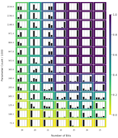
(a) Model A Training

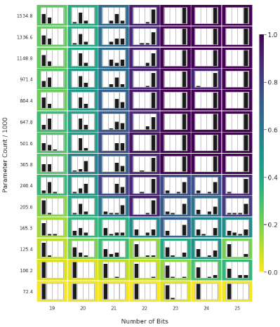
(b) Model A Testing

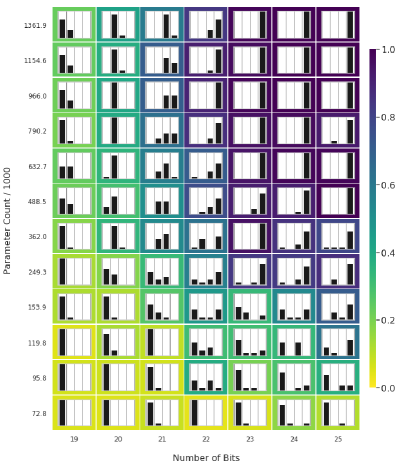
(c) Model B Training

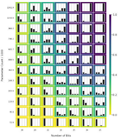
(d) Model B Testing

Figure 8. Efficacy results for models A and B.

References

- (1)
- Andreas (2019) Jacob Andreas. 2019. Measuring Compositionality in Representation Learning. In International Conference on Learning Representations. https://openreview.net/forum?id=HJz05o0qK7
- Bahdanau et al. (2019) Dzmitry Bahdanau, Shikhar Murty, Michael Noukhovitch, Thien Huu Nguyen, Harm de Vries, and Aaron Courville. 2019. Systematic Generalization: What Is Required and Can It Be Learned?. In International Conference on Learning Representations. https://openreview.net/forum?id=HkezXnA9YX
- Baroni (2020) Marco Baroni. 2020. Linguistic generalization and compositionality in modern artificial neural networks. Philosophical Transactions of the Royal Society B: Biological Sciences 375 (02 2020), 20190307. https://doi.org/10.1098/rstb.2019.0307
- Barrett et al. (2018) Jeffrey A. Barrett, Brian Skyrms, and Calvin Cochran. 2018. Hierarchical Models for the Evolution of Compositional Language. http://philsci-archive.pitt.edu/14725/
- Belkin et al. (2019) Mikhail Belkin, Daniel Hsu, Siyuan Ma, and Soumik Mandal. 2019. Reconciling modern machine-learning practice and the classical bias–variance trade-off. Proceedings of the National Academy of Sciences 116, 32 (2019), 15849–15854. https://doi.org/10.1073/pnas.1903070116 arXiv:https://www.pnas.org/content/116/32/15849.full.pdf
- Chaabouni et al. (2019a) Rahma Chaabouni, Eugene Kharitonov, Emmanuel Dupoux, and Marco Baroni. 2019a. Anti-efficient encoding in emergent communication. In Advances in Neural Information Processing Systems 32, H. Wallach, H. Larochelle, A. Beygelzimer, F. d\textquotesingle Alché-Buc, E. Fox, and R. Garnett (Eds.). Curran Associates, Inc., 6290–6300. http://papers.nips.cc/paper/8859-anti-efficient-encoding-in-emergent-communication.pdf
- Chaabouni et al. (2019b) Rahma Chaabouni, Eugene Kharitonov, Alessandro Lazaric, Emmanuel Dupoux, and Marco Baroni. 2019b. Word-order biases in deep-agent emergent communication. arXiv:1905.12330 [cs] (May 2019). arXiv: 1905.12330.
- Chen et al. (2018) Yining Chen, Sorcha Gilroy, Andreas Maletti, Jonathan May, and Kevin Knight. 2018. Recurrent Neural Networks as Weighted Language Recognizers. In Proceedings of the 2018 Conference of the North American Chapter of the Association for Computational Linguistics: Human Language Technologies, Volume 1 (Long Papers). Association for Computational Linguistics, 2261–2271. https://doi.org/10.18653/v1/N18-1205
- Collins et al. (2017) Jasmine Collins, Jascha Sohl-Dickstein, and David Sussillo. 2017. Capacity and Trainability in Recurrent Neural Networks. In International Conference on Learning Representations. https://openreview.net/forum?id=BydARw9ex
- Du et al. (2019) Simon S. Du, Xiyu Zhai, Barnabas Poczos, and Aarti Singh. 2019. Gradient Descent Provably Optimizes Over-parameterized Neural Networks. In International Conference on Learning Representations. https://openreview.net/forum?id=S1eK3i09YQ
- Evtimova et al. (2018) Katrina Evtimova, Andrew Drozdov, Douwe Kiela, and Kyunghyun Cho. 2018. Emergent Communication in a Multi-Modal, Multi-Step Referential Game. In International Conference on Learning Representations. https://openreview.net/forum?id=rJGZq6g0-
- Foerster et al. (2016) Jakob Foerster, Ioannis Alexandros Assael, Nando de Freitas, and Shimon Whiteson. 2016. Learning to Communicate with Deep Multi-Agent Reinforcement Learning. In Advances in Neural Information Processing Systems 29, D. D. Lee, M. Sugiyama, U. V. Luxburg, I. Guyon, and R. Garnett (Eds.). Curran Associates, Inc., 2137–2145. http://papers.nips.cc/paper/6042-learning-to-communicate-with-deep-multi-agent-reinforcement-learning.pdf
- Havrylov and Titov (2017) Serhii Havrylov and Ivan Titov. 2017. Emergence of Language with Multi-agent Games: Learning to Communicate with Sequences of Symbols. In Advances in Neural Information Processing Systems 30, I. Guyon, U. V. Luxburg, S. Bengio, H. Wallach, R. Fergus, S. Vishwanathan, and R. Garnett (Eds.). Curran Associates, Inc., 2149–2159. http://papers.nips.cc/paper/6810-emergence-of-language-with-multi-agent-games-learning-to-communicate-with-sequences-of-symbols.pdf
- Hochreiter and Schmidhuber (1997) Sepp Hochreiter and Jürgen Schmidhuber. 1997. Long Short-Term Memory. Neural Computation 9, 8 (Nov. 1997), 1735–1780. https://doi.org/10.1162/neco.1997.9.8.1735
- Hupkes et al. (2020) Dieuwke Hupkes, Verna Dankers, Mathijs Mul, and Elia Bruni. 2020. The compositionality of neural networks: integrating symbolism and connectionism. Journal of Artificial Intelligence Research (2020).
- Jang et al. (2017) Eric Jang, Shixiang Gu, and Ben Poole. 2017. Categorical Reparameterization with Gumbel-Softmax. In International Conference on Learning Representations. https://openreview.net/forum?id=rkE3y85ee
- Kingma and Ba (2015) Diederik P. Kingma and Jimmy Ba. 2015. Adam: A Method for Stochastic Optimization. In International Conference on Learning Representations.
- Kingma and Welling (2014) Diederik P Kingma and Max Welling. 2014. Auto-encoding Variational Bayes. In International Conference on Learning Representations. https://openreview.net/forum?id=33X9fd2-9FyZd
- Kirby et al. (2015) Simon Kirby, Monica Tamariz, Hannah Cornish, and Kenny Smith. 2015. Compression and Communication in the Cultural Evolution of Linguistic Structure. Cognition 141 (2015), 87–102. https://doi.org/10.1016/j.cognition.2015.03.016
- Kottur et al. (2017) Satwik Kottur, José Moura, Stefan Lee, and Dhruv Batra. 2017. Natural Language Does Not Emerge ‘Naturally’ in Multi-Agent Dialog. In Proceedings of the 2017 Conference on Empirical Methods in Natural Language Processing. Association for Computational Linguistics, 2962–2967. https://doi.org/10.18653/v1/D17-1321
- Lake (2019) Brenden M Lake. 2019. Compositional generalization through meta sequence-to-sequence learning. In Advances in Neural Information Processing Systems 32, H. Wallach, H. Larochelle, A. Beygelzimer, F. d'Alché-Buc, E. Fox, and R. Garnett (Eds.). Curran Associates, Inc., 9788–9798. http://papers.nips.cc/paper/9172-compositional-generalization-through-meta-sequence-to-sequence-learning.pdf
- Lazaridou et al. (2018) Angeliki Lazaridou, Karl Moritz Hermann, Karl Tuyls, and Stephen Clark. 2018. Emergence of Linguistic Communication from Referential Games with Symbolic and Pixel Input. In International Conference on Learning Representations. https://openreview.net/forum?id=HJGv1Z-AW
- Lazaridou et al. (2017) Angeliki Lazaridou, Alexander Peysakhovich, and Marco Baroni. 2017. Multi-Agent Cooperation and the Emergence of (Natural) Language. In International Conference on Learning Representations. https://openreview.net/forum?id=Hk8N3Sclg
- Lee et al. (2019) Jason Lee, Kyunghyun Cho, and Douwe Kiela. 2019. Countering Language Drift via Visual Grounding. In Proceedings of the 2019 Conference on Empirical Methods in Natural Language Processing and the 9th International Joint Conference on Natural Language Processing (EMNLP-IJCNLP). Association for Computational Linguistics, Hong Kong, China, 4376–4386. https://doi.org/10.18653/v1/D19-1447
- Lee et al. (2018) Jason Lee, Kyunghyun Cho, Jason Weston, and Douwe Kiela. 2018. Emergent Translation in Multi-Agent Communication. In International Conference on Learning Representations. https://openreview.net/forum?id=H1vEXaxA-
- Lewis (1969) David Lewis. 1969. Convention: A philosophical study. Harvard University Press.
- Li and Liang (2018) Yuanzhi Li and Yingyu Liang. 2018. Learning Overparameterized Neural Networks via Stochastic Gradient Descent on Structured Data. In Advances in Neural Information Processing Systems 31. Curran Associates, Inc., 8157–8166.
- Liska et al. (2018) Adam Liska, Germán Kruszewski, and Marco Baroni. 2018. Memorize or generalize? Searching for a compositional RNN in a haystack. CoRR abs/1802.06467 (2018). arXiv:1802.06467 http://arxiv.org/abs/1802.06467
- Lowe* et al. (2020) Ryan Lowe*, Abhinav Gupta*, Jakob Foerster, Douwe Kiela, and Joelle Pineau. 2020. On the interaction between supervision and self-play in emergent communication. In International Conference on Learning Representations. https://openreview.net/forum?id=rJxGLlBtwH
- Maddison et al. (2017) Chris J. Maddison, Andriy Mnih, and Yee Whye Teh. 2017. The Concrete Distribution: A Continuous Relaxation of Discrete Random Variables. In International Conference on Learning Representations. https://openreview.net/forum?id=S1jE5L5gl
- Mordatch and Abbeel (2018) Igor Mordatch and Pieter Abbeel. 2018. Emergence of Grounded Compositional Language in Multi-Agent Populations. In AAAI Conference on Artificial Intelligence. https://aaai.org/ocs/index.php/AAAI/AAAI18/paper/view/17007
- Nakkiran et al. (2020) Preetum Nakkiran, Gal Kaplun, Yamini Bansal, Tristan Yang, Boaz Barak, and Ilya Sutskever. 2020. Deep Double Descent: Where Bigger Models and More Data Hurt. In International Conference on Learning Representations. https://openreview.net/forum?id=B1g5sA4twr
- Paszke et al. (2019) Adam Paszke, Sam Gross, Francisco Massa, et al. 2019. PyTorch: An Imperative Style, High-Performance Deep Learning Library. In NeurIPS, H. Wallach, H. Larochelle, A. Beygelzimer, F. d'Alché-Buc, E. Fox, and R. Garnett (Eds.). Curran Associates, Inc., 8024–8035. http://papers.nips.cc/paper/9015-pytorch-an-imperative-style-high-performance-deep-learning-library.pdf
- Spike et al. (2017) Matthew Spike, Kevin Stadler, Simon Kirby, and Kenny Smith. 2017. Minimal Requirements for the Emergence of Learned Signaling. In Cognitive Science. https://doi.org/10.1111/cogs.12351
- Steels (1997) Luc Steels. 1997. The Synthetic Modeling of Language Origins. Evolution of Communication 1, 1 (1997), 1–34. https://doi.org/10.1075/eoc.1.1.02ste
- Steels and Kaplan (2000) Luc Steels and Frédéric Kaplan. 2000. AIBO’s first words: The social learning of language and meaning. Evolution of Communication 4 (2000). http://www.jbe-platform.com/content/journals/10.1075/eoc.4.1.03ste
- Sukhbaatar et al. (2016) Sainbayar Sukhbaatar, Arthur Szlam, and Rob Fergus. 2016. Learning Multiagent Communication with Backpropagation. In NeurIPS, D. D. Lee, M. Sugiyama, U. V. Luxburg, I. Guyon, and R. Garnett (Eds.). Curran Associates, Inc., 2244–2252. http://papers.nips.cc/paper/6398-learning-multiagent-communication-with-backpropagation.pdf
- Verhoef et al. (2016) Tessa Verhoef, Simon Kirby, and Bart de Boer. 2016. Iconicity and the Emergence of Combinatorial Structure in Language. Cognitive Science 40, 8 (2016), 1969–1994. https://doi.org/10.1111/cogs.12326
- Weber et al. (2018) Noah Weber, Leena Shekhar, and Niranjan Balasubramanian. 2018. The Fine Line between Linguistic Generalization and Failure in Seq2Seq-Attention Models. In Proceedings of the Workshop on Generalization in the Age of Deep Learning. Association for Computational Linguistics, 24–27. https://doi.org/10.18653/v1/W18-1004
- Zaslavsky et al. (2018) Noga Zaslavsky, Charles Kemp, Terry Regier, and Naftali Tishby. 2018. Efficient compression in color naming and its evolution. Proceedings of the National Academy of Sciences 115, 31 (July 2018), 7937–7942. https://doi.org/10.1073/pnas.1800521115