Calibration tests in multi-class classification:
A unifying framework

Abstract

In safety-critical applications a probabilistic model is usually required to be calibrated, i.e., to capture the uncertainty of its predictions accurately. In multi-class classification, calibration of the most confident predictions only is often not sufficient. We propose and study calibration measures for multi-class classification that generalize existing measures such as the expected calibration error, the maximum calibration error, and the maximum mean calibration error. We propose and evaluate empirically different consistent and unbiased estimators for a specific class of measures based on matrix-valued kernels. Importantly, these estimators can be interpreted as test statistics associated with well-defined bounds and approximations of the p-value under the null hypothesis that the model is calibrated, significantly improving the interpretability of calibration measures, which otherwise lack any meaningful unit or scale.

1 Introduction

Consider the problem of analyzing microscopic images of tissue samples and reporting a tumour grade, i.e., a score that indicates whether cancer cells are well-differentiated or not, affecting both prognosis and treatment of patients. Since for some pathological images not even experienced pathologists might all agree on one classification, this task contains an inherent component of uncertainty. This type of uncertainty that can not be removed by increasing the size of the training data set is typically called aleatoric uncertainty (Kiureghian and Ditlevsen, 2009). Unfortunately, even if the ideal model is among the class of models we consider, with a finite training data set we will never obtain the ideal model but we can only hope to learn a model that is, in some sense, close to it. Worse still, our model might not even be close to the ideal model if the model class is too restrictive or the number of training data is small—which is not unlikely given the fact that annotating pathological images is expensive. Thus ideally our model should be able to express not only aleatoric uncertainty but also the uncertainty about the model itself. In contrast to aleatoric uncertainty this so-called epistemic uncertainty can be reduced by additional training data.

Dealing with these different types of uncertainty is one of the major problems in machine learning. The application of our model in clinical practice demands “meaningful” uncertainties to avoid doing harm to patients. Being too certain about high tumour grades might cause harm due to unneeded aggressive therapies and overly pessimistic prognoses, whereas being too certain about low tumour grades might result in insufficient therapies. “Proper” uncertainty estimates are also crucial if the model is supervised by a pathologist that takes over if the uncertainty reported by the model is too high. False but highly certain gradings might incorrectly keep the pathologist out of the loop, and on the other hand too uncertain gradings might demand unneeded and costly human intervention.

Probability theory provides a solid framework for dealing with uncertainties. Instead of assigning exactly one grade to each pathological image, so-called probabilistic models report subjective probabilities, sometimes also called confidence scores, of the tumour grades for each image. The model can be evaluated by comparing these subjective probabilities to the ground truth.

One desired property of such a probabilistic model is sharpness (or high accuracy), i.e., if possible, the model should assign the highest probability to the true tumour grade (which maybe can not be inferred from the image at hand but only by other means such as an additional immunohistochemical staining). However, to be able to trust the predictions the probabilities should be calibrated (or reliable) as well (Murphy and Winkler, 1977; DeGroot and Fienberg, 1983). This property requires the subjective probabilities to match the relative empirical frequencies: intuitively, if we could observe a long run of predictions $(0.5,0.1,0.1,0.3)$ for tumour grades $1$, $2$, $3$, and $4$, the empirical frequencies of the true tumour grades should be $(0.5,0.1,0.1,0.3)$. Note that accuracy and calibration are two complementary properties: a model with over-confident predictions can be highly accurate but miscalibrated, whereas a model that always reports the overall proportion of patients of each tumour grade in the considered population is calibrated but highly inaccurate.

Research of calibration in statistics and machine learning literature has been focused mainly on binary classification problems or the most confident predictions: common calibration measures such as the expected calibration error ($\operatorname{ECE}$) (Naeini et al., 2015), the maximum calibration error ($\operatorname{MCE}$) (Naeini et al., 2015), and the kernel-based maximum mean calibration error ($\operatorname{MMCE}$) (Kumar et al., 2018), and reliability diagrams (Murphy and Winkler, 1977) have been developed for binary classification. This is insufficient since many recent applications of machine learning involve multiple classes. Furthermore, the crucial finding of Guo et al. (2017) that many modern deep neural networks are miscalibrated is also based only on the most confident prediction.

Recently Vaicenavicius et al. (2019) suggested that this analysis might be too reduced for many realistic scenarios. In our example, a prediction of $(0.5,0.3,0.1,0.1)$ is fundamentally different from a prediction of $(0.5,0.1,0.1,0.3)$, since according to the model in the first case it is only half as likely that a tumour is of grade 3 or 4, and hence the subjective probability of missing out on a more aggressive therapy is smaller. However, commonly in the study of calibration all predictions with a highest reported confidence score of $0.5$ are grouped together and a calibrated model has only to be correct about the most confident tumour grade in 50% of the cases, regardless of the other predictions. Although the $\operatorname{ECE}$ can be generalized to multi-class classification, its applicability seems to be limited since its histogram-regression based estimator requires partitioning of the potentially high-dimensional probability simplex and is asymptotically inconsistent in many cases (Vaicenavicius et al., 2019). Sample complexity bounds for a bias-reduced estimator of the $\operatorname{ECE}$ introduced in metereological literature (Ferro and Fricker, 2012; Bröcker, 2011) were derived in concurrent work (Kumar et al., 2019).

2 Our contribution

In this work, we propose and study a general framework of calibration measures for multi-class classification. We show that this framework encompasses common calibration measures for binary classification such as the expected calibration error ($\operatorname{ECE}$), the maximum calibration error ($\operatorname{MCE}$), and the maximum mean calibration error ($\operatorname{MMCE}$) by Kumar et al. (2018). In more detail we study a class of measures based on vector-valued reproducing kernel Hilbert spaces, for which we derive consistent and unbiased estimators. The statistical properties of the proposed estimators are not only theoretically appealing, but also of high practical value, since they allow us to address two main problems in calibration evaluation.

As discussed by Vaicenavicius et al. (2019), all calibration error estimates are inherently random, and comparing competing models based on these estimates without taking the randomness into account can be very misleading, in particular when the estimators are biased (which, for instance, is the case for the commonly used histogram-regression based estimator of the $\operatorname{ECE}$). Even more fundamentally, all commonly used calibration measures lack a meaningful unit or scale and are therefore not interpretable as such (regardless of any finite sample issues).

The consistency and unbiasedness of the proposed estimators facilitate comparisons between competing models, and allow us to derive multiple statistical tests for calibration that exploit these properties. Moreover, by viewing the estimators as calibration test statistics, with well-defined bounds and approximations of the corresponding p-value, we give them an interpretable meaning.

We evaluate the proposed estimators and statistical tests empirically and compare them with existing methods. To facilitate multi-class calibration evaluation we provide the Julia packages ConsistencyResampling.jl (Widmann, 2019c), CalibrationErrors.jl (Widmann, 2019a), and CalibrationTests.jl (Widmann, 2019b) for consistency resampling, calibration error estimation, and calibration tests, respectively.

3 Background

We start by shortly summarizing the most relevant definitions and concepts. Due to space constraints and to improve the readability of our paper, we do not provide any proofs in the main text but only refer to the results in the supplementary material, which is intended as a reference for mathematically precise statements and proofs.

3.1 Probabilistic setting

Let $(X,Y)$ be a pair of random variables with $X$ and $Y$ representing inputs (features) and outputs, respectively. We focus on classification problems and hence without loss of generality we may assume that the outputs consist of the $m$ classes $1$, …, $m$.

Let $\Delta^{m}$ denote the $(m-1)$-dimensional probability simplex $\Delta^{m}\coloneqq\{z\in\mathbb{R}_{\geq 0}^{m}\colon\|z\|_{1}=1\}$. Then a probabilistic model $g$ is a function that for every input $x$ outputs a prediction $g(x)\in\Delta^{m}$ that models the distribution

$$\big{(}\operatorname{\mathbb{P}}[Y=1\,|\,X=x],\ldots,\operatorname{\mathbb{P}}[Y=m\,|\,X=x]\big{)}\in\Delta^{m}$$

of class $Y$ given input $X=x$.

3.2 Calibration

3.2.1 Common notion

The common notion of calibration, as, e.g., used by Guo et al. (2017), considers only the most confident predictions $\max_{y}g_{y}(x)$ of a model $g$. According to this definition, a model is calibrated if

$$\operatorname{\mathbb{P}}[Y=\operatorname*{arg\,max}_{y}g_{y}(X)\,|\,\max_{y}g_{y}(X)]=\max_{y}g_{y}(X)$$ (1)

holds almost always. Thus a model that is calibrated according to Eq. 1 ensures that we can partly trust the uncertainties reported by its predictions. As an example, for a prediction of $(0.4,0.3,0.3)$ the model would only guarantee that in the long run inputs that yield a most confident prediction of $40\%$ are in the corresponding class $40\%$ of the time.

3.2.2 Strong notion

According to the more general calibration definition of Bröcker (2009); Vaicenavicius et al. (2019), a probabilistic model $g$ is calibrated if for almost all inputs $x$ the prediction $g(x)$ is equal to the distribution of class $Y$ given prediction $g(X)=g(x)$. More formally, a calibrated model satisfies

$$\operatorname{\mathbb{P}}[Y=y\,|\,g(X)]=g_{y}(X)$$ (2)

almost always for all classes $y\in\{1,\ldots,m\}$. As Vaicenavicius et al. (2019) showed, for multi-class classification this formulation is stronger than the definition of Zadrozny and Elkan (2002) that only demands calibrated marginal probabilities. Thus we can fully trust the uncertainties reported by the predictions of a model that is calibrated according to Eq. 2. The prediction $(0.4,0.3,0.3)$ would actually imply that the class distribution of the inputs that yield this prediction is $(0.4,0.3,0.3)$. To emphasize the difference to the definition in Eq. 1, we call calibration according to Eq. 2 calibration in the strong sense or strong calibration.

To simplify our notation, we rewrite Eq. 2 in vectorized form. Equivalent to the definition above, a model $g$ is calibrated in the strong sense if

$$r(g(X))-g(X)=0$$ (3)

holds almost always, where

$$r(\xi)\coloneqq\big{(}\operatorname{\mathbb{P}}[Y=1\,|\,g(X)=\xi],\ldots,\operatorname{\mathbb{P}}[Y=m\,|\,g(X)=\xi]\big{)}$$

is the distribution of class $Y$ given prediction $g(X)=\xi$.

The calibration of certain aspects of a model, such as the five largest predictions or groups of classes, can be investigated by studying the strong calibration of models induced by so-called calibration lenses. For more details about evaluation and visualization of strong calibration we refer to Vaicenavicius et al. (2019).

3.3 Matrix-valued kernels

The miscalibration measure that we propose in this work is based on matrix-valued kernels $k\colon\Delta^{m}\times\Delta^{m}\to\mathbb{R}^{m\times m}$. Matrix-valued kernels can be defined in a similar way as the more common real-valued kernels, which can be characterized as symmetric positive definite functions (Berlinet and Thomas-Agnan, 2004, Lemma 4).

Definition 1 (Micchelli and Pontil (2005, Definition 2); Caponnetto et al. (2008, Definition 1))

We call a function $k\colon\Delta^{m}\times\Delta^{m}\to\mathbb{R}^{m\times m}$ a matrix-valued kernel if for all $s,t\in\Delta^{m}$ $k(s,t)=k(t,s)^{\intercal}$ and it is positive semi-definite, i.e., if for all $n\in\mathbb{N}$, $t_{1},\ldots,t_{n}\in\Delta^{m}$, and $u_{1},\ldots,u_{n}\in\mathbb{R}^{m}$

$$\sum_{i,j=1}^{n}u_{i}^{\intercal}k(t_{i},t_{j})u_{j}\geq 0.$$

There exists a one-to-one mapping of such kernels and reproducing kernel Hilbert spaces (RKHSs) of vector-valued functions $f\colon\Delta^{m}\to\mathbb{R}^{m}$. We provide a short summary of RKHSs of vector-valued functions on the probability simplex in Appendix D. A more detailed general introduction to RKHSs of vector-valued functions can be found in the publications by Micchelli and Pontil (2005); Carmeli et al. (2010); Caponnetto et al. (2008).

Similar to the scalar case, matrix-valued kernels can be constructed from other matrix-valued kernels and even from real-valued kernels. Very simple matrix-valued kernels are kernels of the form $k(s,t)=\tilde{k}(s,t)\mathbf{I}_{m}$, where $\tilde{k}$ is a scalar-valued kernel, such as the Gaussian or Laplacian kernel, and $\mathbf{I}_{m}$ is the identity matrix. As Example D.1 shows, this construction can be generalized by, e.g., replacing the identity matrix with an arbitrary positive semi-definite matrix.

An important class of kernels are so-called universal kernels. Loosely speaking, a kernel is called universal if its RKHS is a dense subset of the space of continuous functions, i.e., if in the neighbourhood of every continuous function we can find a function in the RKHS. Prominent real-valued kernels on the probability simplex such as the Gaussian and the Laplacian kernel are universal, and can be used to construct universal matrix-valued kernels of the form in Example D.1, as Lemma D.3 shows.

4 Unification of calibration measures

In this section we introduce a general measure of strong calibration and show its relation to other existing measures.

4.1 Calibration error

In the analysis of strong calibration the discrepancy in the left-hand side of Eq. 3 lends itself naturally to the following calibration measure.

Definition 2

Let $\mathcal{F}$ be a non-empty space of functions $f\colon\Delta^{m}\to\mathbb{R}^{m}$. Then the calibration error ($\operatorname{CE}$) of model $g$ with respect to class $\mathcal{F}$ is

$$\operatorname{CE}[\mathcal{F},g]\coloneqq\sup_{f\in\mathcal{F}}\operatorname{\mathbb{E}}\left[{(r(g(X))-g(X))}^{\intercal}f(g(X))\right].$$

A trivial consequence of the design of the $\operatorname{CE}$ is that the measure is zero for every model that is calibrated in the strong sense, regardless of the choice of $\mathcal{F}$. The converse statement is not true in general. As we show in Theorem C.2, the class of continuous functions is a space for which the $\operatorname{CE}$ is zero if and only if model $g$ is strongly calibrated, and hence allows to characterize calibrated models. However, since this space is extremely large, for every model the $\operatorname{CE}$ is either $0$ or $\infty$.. Thus a measure based on this space does not allow us to compare miscalibrated models and hence is rather impractical.

4.2 Kernel calibration error

Due to the correspondence between kernels and RKHSs we can define the following kernel measure.

Definition 3

Let $k$ be a matrix-valued kernel as in Definition 1. Then we define the kernel calibration error ($\operatorname{KCE}$) with respect to kernel $k$ as $\operatorname{KCE}[k,g]\coloneqq\operatorname{CE}[\mathcal{F},g]$, where $\mathcal{F}$ is the unit ball in the RKHS corresponding to kernel $k$.

As mentioned above, a RKHS with a universal kernel is a dense subset of the space of continuous functions. Hence these kernels yield a function space that is still large enough for identifying strongly calibrated models.

Theorem 1 (cf. Theorem C.1).

Let $k$ be a matrix-valued kernel as in Definition 1, and assume that $k$ is universal. Then $\operatorname{KCE}[k,g]=0$ if and only if model $g$ is calibrated in the strong sense.

From the supremum-based Definition 2 it might not be obvious how the $\operatorname{KCE}$ can be evaluated. Fortunately, there exists an equivalent kernel-based formulation.

Lemma 1 (cf. Lemma E.2).

Let $k$ be a matrix-valued kernel as in Definition 1. If $\operatorname{\mathbb{E}}[\|k(g(X),g(X))\|]<\infty$, then

$$\operatorname{KCE}[k,g]={\Big{(}\operatorname{\mathbb{E}}\big{[}{(e_{Y}-g(X))}^{\intercal}k(g(X),g(X^{\prime})){(e_{Y^{\prime}}-g(X^{\prime}))}\big{]}\Big{)}}^{1/2},$$ (4)

where $(X^{\prime},Y^{\prime})$ is an independent copy of $(X,Y)$ and $e_{i}$ denotes the $i$th unit vector.

4.3 Expected calibration error

The most common measure of calibration error is the expected calibration error ($\operatorname{ECE}$). Typically it is used for quantifying calibration in a binary classification setting but it generalizes to strong calibration in a straightforward way. Let $d\colon\Delta^{m}\times\Delta^{m}\to\mathbb{R}_{\geq 0}$ be a distance measure on the probability simplex. Then the expected calibration error of a model $g$ with respect to $d$ is defined as

$$\operatorname{ECE}[d,g]=\operatorname{\mathbb{E}}[d(r(g(X)),g(X))].$$ (5)

If $d(p,q)=0\Leftrightarrow p=q$, as it is the case for standard choices of $d$ such as the total variation distance or the (squared) Euclidean distance, then $\operatorname{ECE}[d,g]$ is zero if and only if $g$ is strongly calibrated as per Eq. 3.

The ECE with respect to the cityblock distance, the total variation distance, or the squared Euclidean distance, are special cases of the calibration error $\operatorname{CE}$, as we show in Lemma I.1.

4.4 Maximum mean calibration error

Kumar et al. (2018) proposed a kernel-based calibration measure, the so-called maximum mean calibration error ($\operatorname{MMCE}$), for training (better) calibrated neural networks. In contrast to their work, in our publication we do not discuss how to obtain calibrated models but focus on the evaluation of calibration and on calibration tests. Moreover, the $\operatorname{MMCE}$ applies only to a binary classification setting whereas our measure quantifies strong calibration and hence is more generally applicable. In fact, as we show in Example I.1, the $\operatorname{MMCE}$ is a special case of the $\operatorname{KCE}$.

5 Calibration error estimators

Consider the task of estimating the calibration error of model $g$ using a validation set $\mathcal{D}=\{(X_{i},Y_{i})\}_{i=1}^{n}$ of $n$ i.i.d. random pairs of inputs and labels that are distributed according to $(X,Y)$.

From the expression for the $\operatorname{ECE}$ in Eq. 5, the natural (and, indeed, standard) approach for estimating the $\operatorname{ECE}$ is as the sample average of the distance $d$ between the predictions $g(X)$ and the calibration function $r(g(X))$. However, this is problematic since the calibration function is not readily available and needs to be estimated as well. Typically, this is addressed using histogram-regression, see, e.g., Guo et al. (2017); Naeini et al. (2015); Vaicenavicius et al. (2019), which unfortunately leads to inconsistent and biased estimators in many cases (Vaicenavicius et al., 2019) and can scale poorly to large $m$. In contrast, for the $\operatorname{KCE}$ in Eq. 4 there is no explicit dependence on $r$, which enables us to derive multiple consistent and also unbiased estimators.

Let $k$ be a matrix-valued kernel as in Definition 1 with $\operatorname{\mathbb{E}}[\|k(g(X),g(X))\|]<\infty$, and define for $1\leq i,j\leq n$

$$h_{i,j}\coloneqq{(e_{Y_{i}}-g(X_{i}))}^{\intercal}k(g(X_{i}),g(X_{j}))(e_{Y_{j}}-g(X_{j})).$$

Then the estimators listed in Table 1 are consistent estimators of the squared kernel calibration error $\operatorname{SKCE}[k,g]\coloneqq\operatorname{KCE}^{2}[k,g]$ (see Lemmas F.1, F.2 and F.3). The subscript letters “q” and “l” refer to the quadratic and linear computational complexity of the unbiased estimators, respectively.

Table 1: Three consistent estimators of the $\operatorname{SKCE}$.

Notation	Definition	Properties	Complexity
$\operatorname{\widehat{SKCE}_{b}}$	$n^{-2}\sum_{i,j=1}^{n}h_{i,j}$	biased	$O(n^{2})$
$\operatorname{\widehat{SKCE}_{uq}}$	${\binom{n}{2}}^{-1}\sum_{1\leq i<j\leq n}h_{i,j}$	unbiased	$O(n^{2})$
$\operatorname{\widehat{SKCE}_{ul}}$	${\lfloor n/2\rfloor}^{-1}\sum_{i=1}^{\lfloor n/2\rfloor}h_{2i-1,2i}$	unbiased	$O(n)$

6 Calibration tests

In general, calibration errors do not have a meaningful unit or scale. This renders it difficult to interpret an estimated non-zero error and to compare different models. However, by viewing the estimates as test statistics with respect to Eq. 3, they obtain an interpretable probabilistic meaning.

Similar to the derivation of the two-sample tests by Gretton et al. (2012), we can use the consistency and unbiasedness of the estimators of the $\operatorname{SKCE}$ presented above to obtain bounds and approximations of the p-value for the null hypothesis $H_{0}$ that the model is calibrated, i.e., for the probability that the estimator is greater than or equal to the observed calibration error estimate, if the model is calibrated. These bounds and approximations do not only allow us to perform hypothesis testing of the null hypothesis $H_{0}$, but they also enable us to transfer unintuitive calibration error estimates to an intuitive and interpretable probabilistic setting.

As we show in Theorems H.2, H.4 and H.3, we can obtain so-called distribution-free bounds without making any assumptions about the distribution of $(X,Y)$ or the model $g$. A downside of these uniform bounds is that usually they provide only a loose bound of the p-value.

Lemma 2 (Distribution-free bounds (see Theorems H.2, H.4 and H.3)).

Let $k$ be a matrix-valued kernel as in Definition 1, and assume that $K_{p;q}\coloneqq\sup_{s,t\in\Delta^{m}}\|k(s,t)\|_{p;q}<\infty$ for some $1\leq p,q\leq\infty$. Let $t>0$ and $B_{p;q}\coloneqq 2^{1+1/p-1/q}K_{p;q}$, then for the biased estimator we can bound

$$\operatorname{\mathbb{P}}\Big{[}\operatorname{\widehat{SKCE}_{b}}\geq t\,\Big{|}\,H_{0}\Big{]}\leq\exp{\bigg{(}-\frac{1}{2}{\Big{(}\max\Big{\{}0,\sqrt{nt/B_{p;q}}-1\Big{\}}\Big{)}}^{2}\bigg{)}},$$

and for either of the unbiased estimators $T\in\{\operatorname{\widehat{SKCE}_{uq}},\operatorname{\widehat{SKCE}_{ul}}\}$, we can bound

$$\operatorname{\mathbb{P}}\Big{[}T\geq t\,\Big{|}\,H_{0}\Big{]}\leq\exp{\bigg{(}-\frac{\lfloor n/2\rfloor t^{2}}{2B_{p;q}^{2}}\bigg{)}}.$$

Asymptotic bounds exploit the asymptotic distribution of the test statistics under the null hypothesis, as the number of validation data points goes to infinity. The central limit theorem implies that the linear estimator is asymptotically normally distributed.

Lemma 3 (Asymptotic distribution of $\operatorname{\widehat{SKCE}_{ul}}$ (see Corollary G.1)).

Let $k$ be a matrix-valued kernel as in Definition 1, and assume that $\operatorname{\mathbb{E}}[\|k(g(X),g(X))\|]<\infty$. If $\operatorname{Var}[h_{i,j}]<\infty$, then

$$\operatorname{\mathbb{P}}\Big{[}\sqrt{\lfloor n/2\rfloor}\operatorname{\widehat{SKCE}_{ul}}\geq t\,\Big{|}\,H_{0}\Big{]}\to 1-\Phi\bigg{(}\frac{t}{\hat{\sigma}}\bigg{)}\quad\text{as}\quad n\to\infty,$$

where $\hat{\sigma}$ is the sample standard deviation of $h_{2i-1,2i}$ ($i=1,\ldots,\lfloor n/2\rfloor$) and $\Phi$ is the cumulative distribution function of the standard normal distribution.

In Theorem G.2 we derive a theoretical expression of the asymptotic distribution of $n\operatorname{\widehat{SKCE}_{uq}}$, under the assumption of strong calibration. This limit distribution can be approximated, e.g., by bootstrapping (Arcones and Giné, 1992) or Pearson curve fitting, as discussed by Gretton et al. (2012).

7 Experiments

We conduct experiments to confirm the derived theoretical properties of the proposed calibration error estimators empirically and to compare them with a standard histogram-regression based estimator of the $\operatorname{ECE}$, denoted by $\widehat{\operatorname{ECE}}$.

We construct synthetic data sets $\{(g(X_{i}),Y_{i})\}_{i=1}^{250}$ of 250 labeled predictions for $m=10$ classes from three generative models. For each model we first sample predictions $g(X_{i})\sim\operatorname{Dir}(0.1,\dots,0.1)$, and then simulate corresponding labels $Y_{i}$ conditionally on $g(X_{i})$ from

$$\mathbf{M1}\colon\,\operatorname{Cat}(g(X_{i})),\quad\mathbf{M2}\colon\,0.5\operatorname{Cat}(g(X_{i}))+0.5\operatorname{Cat}(1,0,\dots,0),\quad\mathbf{M3}\colon\,\operatorname{Cat}(0.1,\dots,0.1),$$

where $\mathbf{M1}$ gives a calibrated model, and $\mathbf{M2}$ and $\mathbf{M3}$ are uncalibrated. In Section J.2 we investigate the theoretical properties of these models in more detail.

For simplicity, we use the matrix-valued kernel $k(x,y)=\exp{(-\|x-y\|/\nu)}\mathbf{I}_{10}$, where the kernel bandwidth $\nu>0$ is chosen by the median heuristic. The total variation distance is a common distance measure of probability distributions and the standard distance measure for the $\operatorname{ECE}$ (Guo et al., 2017; Vaicenavicius et al., 2019; Bröcker and Smith, 2007), and hence it is chosen as the distance measure for all studied calibration errors.

7.1 Calibration error estimates

In Fig. 1 we show the distribution of $\widehat{\operatorname{ECE}}$ and of the three proposed estimators of the $\operatorname{SKCE}$, evaluated on $10^{4}$ randomly sampled data sets from each of the three models. The true calibration error of these models, indicated by a dashed line, is calculated theoretically for the $\operatorname{ECE}$ (see Section J.2.1) and empirically for the $\operatorname{SKCE}$ using the sample mean of all unbiased estimates of $\operatorname{\widehat{SKCE}_{uq}}$. The results confirm the unbiasedness of $\operatorname{\widehat{SKCE}_{ul}}$.

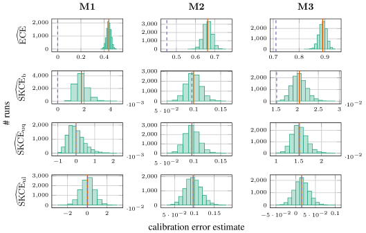
Figure 1: Distribution of calibration error estimates of $10^{4}$ data sets that are randomly sampled from the generative models $\mathbf{M1}$, $\mathbf{M2}$, and $\mathbf{M3}$. The solid line indicates the mean of the calibration error estimates, and the dashed line displays the true calibration error.

7.2 Calibration tests

We repeatedly compute the bounds and approximations of the p-value for the calibration error estimators that were derived in Section 6 on $10^{4}$ randomly sampled data sets from each of the three models. More concretely, we evaluate the distribution-free bounds for $\operatorname{\widehat{SKCE}_{b}}$ ($\mathbf{D}_{\mathrm{b}}$), $\operatorname{\widehat{SKCE}_{uq}}$ ($\mathbf{D}_{\mathrm{uq}}$), and $\operatorname{\widehat{SKCE}_{ul}}$ ($\mathbf{D}_{\mathrm{ul}}$) and the asymptotic approximations for $\operatorname{\widehat{SKCE}_{uq}}$ ($\mathbf{A}_{\mathrm{uq}}$) and $\operatorname{\widehat{SKCE}_{ul}}$ ($\mathbf{A}_{\mathrm{l}}$), where the former is approximated by bootstrapping. We compare them with a previously proposed hypothesis test for the standard $\operatorname{ECE}$ estimator based on consistency resampling ($\mathbf{C}$), in which data sets are resampled under the assumption that the model is calibrated by sampling labels from resampled predictions (Bröcker and Smith, 2007; Vaicenavicius et al., 2019).

For a chosen significance level $\alpha$ we compute from the p-value approximations $p_{1},\ldots,p_{10^{4}}$ the empirical test error

$$\frac{1}{10^{4}}\sum_{i=1}^{10^{4}}\mathbbm{1}_{[0,\alpha]}(p_{i})\quad\text{ (for }\mathbf{M1}\text{)}\qquad\text{and}\qquad\frac{1}{10^{4}}\sum_{i=1}^{10^{4}}\mathbbm{1}_{(\alpha,1]}(p_{i})\quad\text{ (for }\mathbf{M2}\text{ and }\mathbf{M3}\text{)}.$$

In Fig. 2 we plot these empirical test errors versus the significance level.

As expected, the distribution-free bounds seem to be very loose upper bounds of the p-value, resulting in statistical tests without much power. The asymptotic approximations, however, seem to estimate the p-value quite well on average, as can be seen from the overlap with the diagonal in the results for the calibrated model $\mathbf{M1}$ (the empirical test error matches the chosen significance level). Additionally, calibration tests based on asymptotic distribution of these statistics, and in particular of $\operatorname{\widehat{SKCE}_{uq}}$, are quite powerful in our experiments, as the results for the uncalibrated models $\mathbf{M2}$ and $\mathbf{M3}$ show. For the calibrated model, consistency resampling leads to an empirical test error that is not upper bounded by the significance level, i.e., the null hypothesis of the model being calibrated is rejected too often. This behaviour is caused by an underestimation of the p-value on average, which unfortunately makes the calibration test based on consistency resampling for the standard $\operatorname{ECE}$ estimator unreliable.

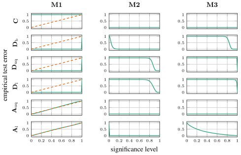
Figure 2: Empirical test error versus significance level for different bounds and approximations of the p-value, evaluated on $10^{4}$ data sets that are randomly sampled from the generative models $\mathbf{M1}$, $\mathbf{M2}$, and $\mathbf{M3}$. The dashed line highlights the diagonal of the unit square.

7.3 Additional experiments

In Section J.2.3 we provide results for varying number of classes and a non-standard $\operatorname{ECE}$ estimator with data-dependent bins. We observe negative and positive bias for both $\operatorname{ECE}$ estimators, whereas $\operatorname{\widehat{SKCE}_{b}}$ is guaranteed to be biased upwards. The bias of $\widehat{\operatorname{ECE}}$ becomes more prominent with increasing number of classes, showing high calibration error estimates even for calibrated models. The $\operatorname{SKCE}$ estimators are not affected by the number of classes in the same way. In some experiments with 100 and 1000 classes, however, the distribution of $\operatorname{\widehat{SKCE}_{ul}}$ shows multi-modality.

The empirical evaluations in Section J.2.4 indicate that the reliability of the p-value approximations based on $\widehat{\operatorname{ECE}}$ decreases with increasing number of classes, both for the estimator with bins of uniform size and, to a smaller extent, for the estimator with data-dependent bins.

The considered calibration measures depend only on the predictions and the true labels, not on how these predictions are computed. Hence directly specifying the predictions allows a clean numerical evaluation and enables comparisons of the estimates with the true calibration error. Nevertheless, we provide a more practical evaluation of calibration for several modern neural networks in Section J.3.

8 Conclusion

We have presented a unified framework for quantifying the calibration error of probabilistic classifiers. The framework encompasses several existing error measures and enables the formulation of a new kernel-based measure. We have derived unbiased and consistent estimators of the kernel-based error measures, which are properties not readily enjoyed by the more common and less tractable $\operatorname{ECE}$. The impact of the kernel and its hyperparameters on the estimators is an important question for future research. We have refrained from investigating it in this paper, since it deserves a more exhaustive study than, what we felt, would have been possible in this work.

The calibration error estimators can be viewed as test statistics. This confers probabilistic interpretability to the error measures. Specifically, we can compute well-founded bounds and approximations of the p-value for the observed error estimates under the null hypothesis that the model is calibrated. We have derived distribution-free bounds and asymptotic approximations for the estimators of the proposed kernel-based error measure, that allow reliable calibration tests in contrast to previously proposed tests based on consistency resampling with the standard estimator of the $\operatorname{ECE}$.

Acknowledgements

We thank the reviewers for all the constructive feedback on our paper. This research is financially supported by the Swedish Research Council via the projects Learning of Large-Scale Probabilistic Dynamical Models (contract number: 2016-04278) and Counterfactual Prediction Methods for Heterogeneous Populations (contract number: 2018-05040), by the Swedish Foundation for Strategic Research via the project Probabilistic Modeling and Inference for Machine Learning (contract number: ICA16-0015), and by the Wallenberg AI, Autonomous Systems and Software Program (WASP) funded by the Knut and Alice Wallenberg Foundation.

Appendix A Notation

We introduce some additional notation to keep the following discussion concise.

Let $U$ be a compact metric space and $V$ be a Hilbert space. In this paper we only consider $U=[0,1]$ and $U=\Delta^{m}$. By $\mathcal{C}(U,V)$ we denote the space of continuous functions $f\colon U\to V$.

For $1\leq p<\infty$, $L^{p}(U,\mu;V)$ is the space of (equivalence classes of) measurable functions $f\colon U\to V$ such that $\|f\|^{p}$ is $\mu$-integrable, equipped with norm $\|f\|_{\mu,p}={(\int_{U}\|f(x)\|^{p}\,\mu(\mathrm{d}x))}^{1/p}$; for $p=\infty$, $L^{\infty}(U,\mu;V)$ is the space of $\mu$-essentially bounded measurable functions $f\colon U\to V$ with norm $\|f\|_{\mu,\infty}=\mu\text{-}\operatorname*{ess\,sup}_{x\in\mathcal{X}}\|f(x)\|$. We denote the closed unit ball of the space $L^{p}(U,\mu;V)$ by $K^{p}(U,\mu;V)\coloneqq\{f\in L^{p}(U,\mu;V)\colon\|f\|_{\mu,p}\leq 1\}$.

If the norm $\|.\|_{V}$ on $V$ is not clear from the context we indicate it by writing $L^{p}(U,\mu;V,\|.\|_{V})$, $K^{p}(U,\mu;V,\|.\|_{V})$, and $\|.\|_{\mu,p;\|.\|_{V}}$. If $V\subset\mathbb{R}^{d}$, all possible norms $\|.\|_{V}$ are equivalent and hence we choose $\|.\|_{p}$ on $V$ to simplify our calculations, if not stated otherwise. Moreover, if $V\subset\mathbb{R}^{d}$ and $\|.\|_{V}=\|.\|_{q}$ for some $1\leq q\leq\infty$, for convenience we write $\|.\|_{\mu,p;q}=\|.\|_{\mu,p;\|.\|_{V}}$.

Let $W$ be another Hilbert space. Then $\mathcal{L}(V,W)$ denotes the space of bounded linear operators $T\colon V\to W$; if $W=V$, we write $\mathcal{L}(V)\coloneqq\mathcal{L}(V,V)$. The induced operator norm on $\mathcal{L}(V,W)$ is defined by

$$\begin{split}\|T\|_{\|.\|_{V};\|.\|_{W}}&=\inf\{c\geq 0\colon\|Tv\|_{W}\leq c\|v\|_{V}\text{for all }v\in V\}\\ &=\sup_{v\in V\colon\|v\|_{V}\leq 1}\|Tv\|_{W}.\end{split}$$

If $W=V$, we write $\|.\|_{\|.\|_{V}}=\|.\|_{\|.\|_{V};\|.\|_{V}}$. Moreover, for convenience if $V\subset\mathbb{R}^{d}$ and $\|.\|_{V}=\|.\|_{p}$ for some $1\leq p\leq\infty$, we use the notation $\|.\|_{p;\|.\|_{W}}=\|.\|_{\|.\|_{V};\|.\|_{W}}$. In the same way, if $W\subset\mathbb{R}^{d}$ and $\|.\|_{W}=\|.\|_{q}$ for some $1\leq q\leq\infty$, we write $\|.\|_{\|.\|_{V};q}=\|.\|_{\|.\|_{V};\|.\|_{W}}$.

By $\mathcal{B}(T)$ we denote the Borel $\sigma$-algebra of a topological space $T$.

We write $\mu_{A}$ for the distribution of a random variable $A$, i.e., the pushforward measure it induces, if $A$ is defined on a probability space with probability measure $\mu$.

Appendix B Probabilistic setting

Let $(\Omega,\mathcal{A},\mu)$ be a probability space. Let $m\in\mathbb{N}$ and define the random variables $X\colon(\Omega,\mathcal{A})\to(\mathcal{X},\Sigma_{X})$ and $Y\colon(\Omega,\mathcal{A})\to(\{1,\ldots,m\},2^{\{1,\ldots,m\}})$, such that $\Sigma_{X}$ contains all singletons. We denote a version of the regular conditional distribution of $Y$ given $X$ by $\mu_{Y|X}(\cdot|x)$ for all $x\in\mathcal{X}$.

We consider the problem of learning a measurable function $g\colon(\mathcal{X},\Sigma_{X})\to(\Delta^{m},\mathcal{B}(\Delta^{m}))$ that returns the prediction $g_{y}(x)$ of $\mu_{Y|X}(\{y\}|x)$ for all $x\in\mathcal{X}$ and $y\in\{1,\ldots,m\}$. We define the random variable $G\colon(\Omega,\mathcal{A})\to(\Delta^{m},\mathcal{B}(\Delta^{m}))$ as $G\coloneqq g(X)$.

In the same way as above, we denote a version of the regular conditional distribution of $Y$ given $G$ by $\mu_{Y|G}(\cdot|t)$ for all $t\in\Delta^{m}$. The function $\delta\colon(\Delta^{m},\mathcal{B}(\Delta^{m}))\to(\mathbb{R}^{m},\mathcal{B}(\mathbb{R}^{m}))$, given by

$$\delta(t)\coloneqq\begin{pmatrix}\mu_{Y|G}(1|t)-t\\ \vdots\\ \mu_{Y|G}(m|t)-t\end{pmatrix}$$

for all $t\in\Delta^{m}$, gives rise to another random variable $\Delta\colon(\Omega,\mathcal{A})\to(\mathbb{R}^{m},\mathcal{B}(\mathbb{R}^{m}))$ that is defined by $\Delta\coloneqq\delta(G)$.

Using the newly introduced mathematical notation, we can reformulate strong calibration in a compact way. A model $g$ is calibrated in the strong sense if $\mu_{Y|G}(\cdot|G)=G$ almost surely, or equivalently if $\Delta=0$ almost surely.

Appendix C Calibration error

Definition C.1 (Calibration error)

Let $\mathcal{F}\subset L^{1}(\Delta^{m},\mu_{G};\mathbb{R}^{m})$ be non-empty. Then the calibration error $\operatorname{CE}$ of model $g$ with respect to class $\mathcal{F}$ is

$$\operatorname{CE}[\mathcal{F},g]\coloneqq\sup_{f\in\mathcal{F}}\operatorname{\mathbb{E}}\left[\langle\Delta,f(G)\rangle_{\mathbb{R}^{m}}\right].$$

Remark C.1

Note that $\|\Delta\|_{\infty}\leq 1$ almost surely, and thus $\|\delta\|_{\mu_{G},\infty}\leq 1$. Hence by Hölder’s inequality for all $f\in\mathcal{F}$ we have

$$|\operatorname{\mathbb{E}}[\langle\Delta,f(G)\rangle_{\mathbb{R}^{m}}]|\leq\operatorname{\mathbb{E}}[|\langle\Delta,f(G)\rangle_{\mathbb{R}^{m}}|]\leq\|\delta\|_{\mu_{G},\infty}\|f\|_{\mu_{G},1}\leq\|f\|_{\mu_{G},1}<\infty.$$

However, it is still possible that $\operatorname{CE}[\mathcal{F},g]=\infty$.

Remark C.2

If $\mathcal{F}$ is symmetric in the sense that $f\in\mathcal{F}$ implies $-f\in\mathcal{F}$, then $\operatorname{CE}[\mathcal{F},g]\geq 0$.

The measure highly depends on the choice of $\mathcal{F}$ but strong calibration always implies a calibration error of zero.

Theorem C.1 (Strong calibration implies zero error).

Let $\mathcal{F}\subset L^{1}(\Delta^{m},\mu_{G};\mathbb{R})$. If model $g$ is calibrated in the strong sense, then $\operatorname{CE}[\mathcal{F},g]=0$.

Proof.

If model $g$ is calibrated in the strong sense, then $\Delta=0$ almost surely. Hence for all $f\in\mathcal{F}$ we have $\operatorname{\mathbb{E}}[\langle\Delta,f(G)\rangle_{\mathbb{R}}]=0$, which implies $\operatorname{CE}[\mathcal{F},g]=0$. ∎

Of course, the converse statement is not true in general. A similar result as above shows that the class of continuous functions, albeit too large and impractical, allows to identify calibrated models.

Theorem C.2.

Let $\mathcal{F}=\mathcal{C}(\Delta^{m},\mathbb{R}^{m})$. Then $\operatorname{CE}[\mathcal{F},g]=0$ if and only if model $g$ is calibrated in the strong sense.

Proof.

Note that $\mathcal{F}$ is well defined since $\mathcal{F}\subset L^{1}(\Delta^{m},\mu_{G};\mathbb{R}^{m})$.

If model $g$ is calibrated in the strong sense, then $\operatorname{CE}[\mathcal{F},g]=0$ by Theorem C.1.

If model $g$ is not calibrated in the strong sense, then $\Delta=0$ does not hold almost surely. In particular, there exists $s\in\{-1,1\}^{m}$ such that $\langle\Delta,s\rangle_{\mathbb{R}^{m}}\leq 0$ does not hold almost surely. Define the function $f_{s}\colon\Delta^{m}\to\mathbb{R}^{m}$ by $f_{s}\coloneqq\langle\delta(\cdot),s\rangle_{\mathbb{R}^{m}}$ and let $A_{s}\coloneqq f_{s}^{-1}((0,\infty))$. Then $A_{s}\in\mathcal{B}(\Delta^{m})$ since $f_{s}$ is Borel measurable, and $\mu_{G}(A_{s})>0$. Hence we know that

$$\alpha_{s}\coloneqq\operatorname{\mathbb{E}}[\langle\Delta,s\mathbbm{1}_{A_{s}}(G)\rangle_{\mathbb{R}^{m}}]>0.$$

Since $\mu_{G}$ is a Borel probability measure on a compact metric space, it is regular and hence there exist a compact set $K$ and an open set $U$ such that $K\subset A_{s}\subset U$ and $\mu_{G}(U\setminus K)<\alpha_{s}/4$ (Rudin, 1986, Theorem 2.17). Thus by Urysohn’s lemma applied to the closed sets $K$ and $U^{c}$, there exists a continuous function $h\in\mathcal{C}(\Delta^{m},\mathbb{R})$ such that $\mathbbm{1}_{K}\leq h\leq\mathbbm{1}_{U}$. By defining $f=sh\in\mathcal{C}(\Delta^{m},\mathbb{R}^{m})$ and applying Hölder’s inequality we obtain

$$\begin{split}\operatorname{\mathbb{E}}[\langle\Delta,f(G)\rangle_{\mathbb{R}^{m}}]&=\operatorname{\mathbb{E}}[\langle\Delta,s\mathbbm{1}_{A_{s}}(G)\rangle_{\mathbb{R}^{m}}]\\ &\quad+\operatorname{\mathbb{E}}[\langle\Delta,f(G)-s\mathbbm{1}_{A_{s}}(G)\rangle_{\mathbb{R}^{m}}]\\ &\geq\alpha_{s}-|\operatorname{\mathbb{E}}[(h(G)-\mathbbm{1}_{A_{s}}(G))\langle\Delta,s\rangle_{\mathbb{R}^{m}}]|\\ &\geq\alpha_{s}-\operatorname{\mathbb{E}}[|h(G)-\mathbbm{1}_{A_{s}}(G)||\langle\Delta,s\rangle_{\mathbb{R}^{m}}|]\\ &\geq\alpha_{s}-\operatorname{\mathbb{E}}[\mathbbm{1}_{U\setminus K}(G)\|\Delta\|_{1}\|s\|_{\infty}]\geq\alpha_{s}-2\mu_{G}(U\setminus K)\\ &>\alpha_{s}-\alpha_{s}/2=\alpha_{s}/2>0.\end{split}$$

This implies $\operatorname{CE}[\mathcal{F},g]>0$. ∎

Appendix D Reproducing kernel Hilbert spaces of vector-valued functions on the probability simplex

Definition D.1 (Micchelli and Pontil (2005, Definition 1))

Let $\mathcal{H}$ be a Hilbert space of vector-valued functions $f\colon\Delta^{m}\to\mathbb{R}^{m}$ with inner product $\langle.,.\rangle_{\mathcal{H}}$. We call $\mathcal{H}$ a reproducing kernel Hilbert space (RKHS), if for all $t\in\Delta^{m}$ and $u\in\mathbb{R}^{m}$ the functional $E_{t,u}\colon\mathcal{H}\to\mathbb{R}$, $E_{t,u}f\coloneqq\langle u,f(t)\rangle_{\mathbb{R}^{m}}$, is a bounded (or equivalently continuous) linear operator.

Riesz’s representation theorem ensures that there exists a unique function $k\colon\Delta^{m}\times\Delta^{m}\to\mathbb{R}^{m\times m}$ such that for all $t\in\Delta^{m}$ the function $k(\cdot,t)$ is a linear map from $\Delta^{m}$ to $\mathcal{H}$ and for all $u\in\mathbb{R}^{m}$ it satisfies the so-called reproducing property

$$\langle u,f(t)\rangle_{\mathbb{R}^{m}}=E_{t,u}f=\langle k(\cdot,t)u,f\rangle_{\mathcal{H}}.$$ (D.1)

It can be shown that function $k$ is self-adjoint and positive semi-definite, and hence a kernel according to Definition 1 (Micchelli and Pontil, 2005, Proposition 1). Similar to the scalar-valued case, conversely by the Moore-Aronszaijn theorem (Aronszajn, 1950) to every kernel $k\colon\Delta^{m}\times\Delta^{m}\to\mathcal{L}(\mathbb{R}^{m})$ there exists a unique RKHS $\mathcal{H}\subset{(\mathbb{R}^{m})}^{\Delta^{m}}$ with $k$ as reproducing kernel (Micchelli and Pontil, 2005, Theorem 1).

Other useful properties are summarized in Lemma D.1. Micchelli and Pontil (2005) considered only the Euclidean norm on $\mathbb{R}^{m}$, corresponding to $p=q=2$ in our statement. For convenience we use the notation $\|.\|_{p;\mathcal{H}}=\|.\|_{\|.\|_{p};\|.\|_{\mathcal{H}}}$.

Lemma D.1 (Micchelli and Pontil (2005, Proposition 1)).

Let $\mathcal{H}\subset{(\mathbb{R}^{m})}^{\Delta^{m}}$ be a RKHS with kernel $k\colon\Delta^{m}\times\Delta^{m}\to\mathcal{L}(\mathbb{R}^{m})$. Let $1\leq p,q\leq\infty$ with Hölder conjugates $p^{\prime}$ and $q^{\prime}$, respectively.

1. For all $t\in\Delta^{m}$

   $$\|k(\cdot,t)\|_{p;\mathcal{H}}={\|k(t,t)\|}^{1/2}_{p;p^{\prime}}.$$ (D.2)

2. For all $s,t\in\Delta^{m}$

   $$\|k(s,t)\|_{p;q}\leq\|k(s,s)\|_{q^{\prime};q}^{1/2}\|k(t,t)\|_{p;p^{\prime}}^{1/2}.$$ (D.3)

3. For all $f\in\mathcal{H}$ and $t\in\Delta^{m}$

   $$\|f(t)\|_{p}\leq\|f\|_{\mathcal{H}}\|k(\cdot,t)\|_{p^{\prime};\mathcal{H}}=\|f\|_{\mathcal{H}}{\|k(t,t)\|}^{1/2}_{p^{\prime};p}.$$ (D.4)

Proof.

Let $t\in\Delta^{m}$. From the reproducing property, Hölder’s inequality, and the definition of the operator norm, we obtain for all $u\in\mathbb{R}^{m}$

$$\|k(\cdot,t)u\|_{\mathcal{H}}^{2}=\langle k(\cdot,t)u,k(\cdot,t)u\rangle_{\mathcal{H}}=\langle u,k(t,t)u\rangle_{\mathbb{R}^{m}}\leq\|u\|_{p}\|k(t,t)u\|_{p^{\prime}}\leq{\|u\|}^{2}_{p}\|k(t,t)\|_{p;p^{\prime}},$$

which implies that

$$\|k(\cdot,t)\|_{p;\mathcal{H}}=\sup_{u\in\mathbb{R}^{m}\setminus\{0\}}\frac{\|k(\cdot,t)u\|_{\mathcal{H}}}{\|u\|_{p}}\leq\|k(t,t)\|_{p;p^{\prime}}^{1/2}.$$ (D.5)

On the other hand, for all $u,v\in\mathbb{R}^{m}$ it follows from the reproducing property, the Cauchy-Schwarz inequality, and the definition of the operator norm that

$$\langle u,k(t,t)v\rangle_{\mathbb{R}^{m}}=\langle k(\cdot,t)u,k(\cdot,t)v\rangle_{\mathcal{H}}\leq\|k(\cdot,t)u\|_{\mathcal{H}}\|k(\cdot,t)v\|_{\mathcal{H}}\leq\|u\|_{p}\|v\|_{p}\|k(\cdot,t)\|^{2}_{p;\mathcal{H}}.$$

Since the $\ell_{p}$-norm is the dual norm of the $\ell_{p^{\prime}}$-norm, it follows that

$$\|k(t,t)v\|_{p^{\prime}}=\sup_{u\in\mathbb{R}^{m}\colon\|u\|_{p}\leq 1}\langle u,k(t,t)v\rangle_{\mathbb{R}^{m}}\leq\|v\|_{p}\|k(\cdot,t)\|^{2}_{p;\mathcal{H}},$$

which implies that

$$\|k(t,t)\|_{p;p^{\prime}}=\sup_{v\in\mathbb{R}^{m}\setminus\{0\}}\frac{\|k(t,t)v\|_{p^{\prime}}}{\|v\|_{p}}\leq\|k(\cdot,t)\|^{2}_{p;\mathcal{H}}.$$ (D.6)

Equation D.2 follows from Eqs. D.5 and D.6.

Let $s,t\in\Delta^{m}$. From the reproducing property, the Cauchy-Schwarz inequality, and the definition of the operator norm, we get for all $u,v\in\mathbb{R}^{m}$

$$\begin{split}\langle u,k(s,t)v\rangle_{\mathbb{R}^{m}}&\leq\langle k(\cdot,s)u,k(\cdot,t)v\rangle_{\mathcal{H}}\leq\|k(\cdot,s)u\|_{\mathcal{H}}\|k(\cdot,t)v\|_{\mathcal{H}}\\ &\leq\|u\|_{q^{\prime}}\|v\|_{p}\|k(\cdot,s)\|_{q^{\prime};\mathcal{H}}\|k(\cdot,t)\|_{p;\mathcal{H}}.\end{split}$$

Thus we obtain

$$\|k(s,t)v\|_{q}=\sup_{u\in\mathbb{R}^{m}\colon\|u\|_{q^{\prime}}\leq 1}\langle u,k(s,t)v\rangle_{\mathbb{R}^{m}}\leq\|v\|_{p}\|k(\cdot,s)\|_{q^{\prime};\mathcal{H}}\|k(\cdot,t)\|_{p;\mathcal{H}},$$

which implies

$$\|k(s,t)\|_{p;q}=\sup_{v\in\mathbb{R}^{m}\setminus\{0\}}\frac{\|k(s,t)v\|_{q}}{\|v\|_{p}}\leq\|k(\cdot,s)\|_{q^{\prime};\mathcal{H}}\|k(\cdot,t)\|_{p;\mathcal{H}}.$$

Hence from Eq. D.2 we obtain Eq. D.3.

For the third statement, let $f\in\mathcal{H}$ and $t\in\Delta^{m}$. From the reproducing property, the Cauchy-Schwarz inequality, and the definition of the operator norm, we obtain for all $u\in\mathbb{R}^{m}$

$$\langle u,f(t)\rangle_{\mathbb{R}^{m}}=\langle k(\cdot,t)u,f\rangle_{\mathcal{H}}\leq\|k(\cdot,t)u\|_{\mathcal{H}}\|f\|_{\mathcal{H}}\leq\|u\|_{p^{\prime}}\|k(\cdot,t)\|_{p^{\prime};\mathcal{H}}\|f\|_{\mathcal{H}}.$$

Thus the duality of the $\ell_{p}$- and the $\ell_{p^{\prime}}$-norm implies

$$\|f(t)\|_{p}=\sup_{u\in\mathbb{R}^{m}\colon\|u\|_{p^{\prime}}\leq 1}\langle u,f(t)\rangle_{\mathbb{R}^{m}}\leq\|k(\cdot,t)\|_{p^{\prime};\mathcal{H}}\|f\|_{\mathcal{H}},$$

which together with Eq. D.2 yields Eq. D.4. ∎

If $\mu$ is a measure on $\Delta^{m}$, we define for $1\leq p,q\leq\infty$ $\|k\|_{\mu,p;q}\coloneqq\|\tilde{k}_{q}\|_{\mu,p}$ where $\tilde{k}_{q}\colon\Delta^{m}\to\mathbb{R}$ is given by $\tilde{k}(t)\coloneqq\|k(\cdot,t)\|_{q;\mathcal{H}}=\|k(t,t)\|_{q;q^{\prime}}^{1/2}$. We omit the value of $q$ if it is clear from the context or does not matter, since all norms on $\mathbb{R}^{m}$ are equivalent.

It is possible to construct certain classes of matrix-valued kernels from scalar-valued kernels, as the following example shows.

Example D.1 (Micchelli and Pontil (2005); Caponnetto et al. (2008, Example 1))

For all $i\in\{1,\ldots,n\}$, let $k_{i}\colon\Delta^{m}\times\Delta^{m}\to\mathbb{R}$ be a scalar-valued kernel and $A_{i}\in\mathbb{R}^{m\times m}$ be a positive semi-definite matrix. Then the function

$$k\colon\Delta^{m}\times\Delta^{m}\to\mathbb{R}^{m\times m},\qquad k(s,t)\coloneqq\sum_{i=1}^{n}k_{i}(s,t)A_{i},$$ (D.7)

is a matrix-valued kernel.

We state a simple result about measurability of functions in the considered RKHSs. The result can be formulated in a much more general fashion and is similar to a result by Christmann and Steinwart (2008, Lemma 4.24).

Lemma D.2 (Measurable RKHS).

Let $\mathcal{H}\subset{(\mathbb{R}^{m})}^{\Delta^{m}}$ be a RKHS with kernel $k\colon\Delta^{m}\times\Delta^{m}\to\mathcal{L}(\mathbb{R}^{m})$. Then all $f\in\mathcal{H}$ are measurable if and only if $k(\cdot,t)u\in{(\mathbb{R}^{m})}^{\Delta^{m}}$ is measurable for all $t\in\Delta^{m}$ and $u\in\mathbb{R}^{m}$.

Proof.

If all $f\in\mathcal{H}$ are measurable, then $k(\cdot,t)u\in\mathcal{H}$ is measurable for all $t\in\Delta^{m}$ and $u\in\mathbb{R}^{m}$.

If $k(\cdot,t)u$ is measurable for all $t\in\Delta^{m}$ and $u\in\mathbb{R}^{m}$, then all functions in $\mathcal{H}_{0}\coloneqq\operatorname{span}{\{k(\cdot,t)u\colon t\in\Delta^{m},u\in\mathbb{R}^{m}\}}\subset\mathcal{H}$ are measurable.

Let $f\in\mathcal{H}$. Since $\mathcal{H}=\overline{\mathcal{H}}_{0}$ (see, e.g., Carmeli et al., 2010), there exists a sequence $(f_{n})_{n\in\mathbb{N}}\subset\mathcal{H}_{0}$ such that $\lim_{n\to\infty}\|f-f_{n}\|_{\mathcal{H}}=0$. For all $t\in\Delta^{m}$, since the operator $k^{*}(\cdot,t)$ is continuous, by the reproducing property we obtain $\lim_{n\to\infty}f_{n}(t)=f(t)$. Thus $f$ is measurable. ∎

By definition (see, e.g., Carmeli et al., 2010, Definition 1), a RKHS with a continuous kernel is a subspace of the space of continuous functions. The following equivalent formulation is an immediate consequence of the result by Carmeli et al. (2010).

Corollary D.1 (Carmeli et al. (2010, Proposition 1)).

A kernel $k\colon\Delta^{m}\times\Delta^{m}\to\mathbb{R}^{m}$ is continuous if for all $t\in\Delta^{m}$ $t\mapsto\|k(t,t)\|$ is bounded and for all $t\in\Delta^{m}$ and $u\in\mathbb{R}^{m}$ $k(\cdot,t)u$ is a continuous function from $\Delta^{m}$ to $\mathbb{R}^{m}$.

An important class of continuous kernels are so-called universal kernels, for which the corresponding RKHS is a dense subset of the space of continuous functions with respect to the uniform norm. A result by Caponnetto et al. (2008) shows under what assumptions matrix-valued kernels of the form in Example D.1 are universal.

Lemma D.3 (Caponnetto et al. (2008, Theorem 14)).

For all $i\in\{1,\ldots,n\}$, let $k_{i}\colon\Delta^{m}\times\Delta^{m}\to\mathbb{R}$ be a universal scalar-valued kernel and $A_{i}\in\mathbb{R}^{m\times m}$ be a positive semi-definite matrix. Then the matrix-valued kernel defined in Eq. D.7 is universal if and only if $\sum_{i=1}^{n}A_{i}$ is positive definite.

Appendix E Kernel calibration error

The one-to-one correspondence between matrix-valued kernels and RKHSs of vector-valued functions motivates the introduction of the kernel calibration error ($\operatorname{KCE}$) in Definition 3. For certain kernels we are able to identify strongly calibrated models.

Theorem E.1.

Let $k\colon\Delta^{m}\times\Delta^{m}\to\mathcal{L}(\mathbb{R}^{m})$ be a universal continuous kernel. Then $\operatorname{KCE}[k,g]=0$ if and only if model $g$ is calibrated in the strong sense.

Proof.

Let $\mathcal{F}$ be the unit ball in the RKHS $\mathcal{H}\subset{(\mathbb{R}^{m})}^{\Delta^{m}}$ corresponding to kernel $k$. Since kernel $k$ is continuous, by definition $\mathcal{H}\subset\mathcal{C}(\Delta^{m},\mathbb{R}^{m})$ (Carmeli et al., 2010, Definition 1). Thus $\mathcal{F}$ is well defined since $\mathcal{F}\subset\mathcal{C}(\Delta^{m},\mathbb{R}^{m})\subset L^{1}(\Delta^{m},\mu_{G};\mathbb{R}^{m})$.

If $g$ is calibrated in the strong sense, it follows from Theorem C.1 that $\operatorname{KCE}[k,g]=\operatorname{CE}[\mathcal{F},g]=0$.

Assume that $\operatorname{KCE}[k,g]=\operatorname{CE}[\mathcal{F},g]=0$. This implies $\operatorname{\mathbb{E}}[\langle\Delta,f(G)\rangle_{\mathbb{R}^{m}}]=0$ for all $f\in\mathcal{F}$. Let $f\in\mathcal{C}(\Delta^{m},\mathbb{R}^{m})$. Since $\mathcal{H}$ is dense in $\mathcal{C}(\Delta^{m},\mathbb{R}^{m})$ (Carmeli et al., 2010, Theorem 1), for all $\epsilon>0$ there exists a function $h\in\mathcal{H}$ with $\|f-h\|_{\infty}<\epsilon/2$. Define $\tilde{h}\in\mathcal{F}$ by $\tilde{h}\coloneqq h/\|h\|_{\mathcal{H}}$ if $\|h\|_{\mathcal{H}}\neq 0$ and $\tilde{h}\coloneqq h$ otherwise. Since

$$\operatorname{\mathbb{E}}[\langle\Delta,h(G)\rangle_{\mathbb{R}^{m}}]=\|h\|_{\mathcal{H}}\operatorname{\mathbb{E}}[\langle\Delta,\tilde{h}(G)\rangle_{\mathbb{R}^{m}}]=0,$$

by Hölder’s inequality we obtain

$$\begin{split}|\operatorname{\mathbb{E}}[\langle\Delta,f(G)\rangle_{\mathbb{R}^{m}}]|&=|\operatorname{\mathbb{E}}[\langle\Delta,f(G)-h(G)\rangle_{\mathbb{R}^{m}}]|\\ &\leq\operatorname{\mathbb{E}}[|\langle\Delta,f(G)-h(G)\rangle_{\mathbb{R}^{m}}|]\\ &\leq\|\delta\|_{\mu_{G},1}\|f-h\|_{\mu_{G},\infty}\\ &\leq 2\|f-h\|_{\infty}<\epsilon.\end{split}$$

Thus $\operatorname{CE}[\mathcal{C}(\Delta^{m},\mathbb{R}^{m}),g]=0$, and hence $g$ is calibrated in the strong sense by Theorem C.2. ∎

Similar to the maximum mean discrepancy (Gretton et al., 2012), if we consider functions in a RKHS, we can rewrite the expectation $\operatorname{\mathbb{E}}[\langle\Delta,f(G)\rangle_{\mathbb{R}^{m}}]$ as an inner product in the Hilbert space.

Lemma E.1 (Existence and uniqueness of embedding).

Let $\mathcal{H}\subset{(\mathbb{R}^{m})}^{\Delta^{m}}$ be a RKHS with kernel $k\colon\Delta^{m}\times\Delta^{m}\to\mathcal{L}(\mathbb{R}^{m})$, and assume that $k(\cdot,t)u$ is measurable for all $t\in\Delta^{m}$ and $u\in\mathbb{R}^{m}$, and $\|k\|_{\mu_{G},1}<\infty$.

Then there exists a unique embedding $\mu_{g}\in\mathcal{H}$ such that for all $f\in\mathcal{H}$

$$\operatorname{\mathbb{E}}[\langle\Delta,f(G)\rangle_{\mathbb{R}^{m}}]=\langle f,\mu_{g}\rangle_{\mathcal{H}}.$$

The embedding $\mu_{g}$ satisfies for all $t\in\Delta^{m}$ and $y\in\mathbb{R}^{m}$

$$\langle y,\mu_{g}(t)\rangle_{\mathbb{R}^{m}}=\operatorname{\mathbb{E}}[\langle\Delta,k(G,t)y\rangle_{\mathbb{R}^{m}}].$$

Proof.

By Lemma D.2 all $f\in\mathcal{H}$ are measurable. Moreover, by Eq. D.4 for all $f\in\mathcal{H}$ we have

$$\begin{split}\int_{\Delta^{m}}\|f(t)\|_{1}\mu_{G}(\mathrm{d}t)&\leq\|f\|_{\mathcal{H}}\int_{\Delta^{m}}{\|k(t,t)\|}_{\infty;1}^{1/2}\,\mu_{G}(\mathrm{d}t)\\ &=\|f\|_{\mathcal{H}}\|k\|_{\mu_{G},1;\infty}<\infty,\end{split}$$

and thus $\mathcal{H}\subset L^{1}(\Delta^{m},\mu_{G};\mathbb{R}^{m})$. Hence from Remark C.1 (with $\mathcal{F}=\mathcal{H}$) we know that for all $f\in\mathcal{H}$ the expectation $\operatorname{\mathbb{E}}[\langle\Delta,f(G)\rangle_{\mathbb{R}^{m}}]$ exists and is finite.

Define the linear operator $T_{g}\colon\mathcal{H}\to\mathbb{R}$ by $T_{g}f\coloneqq\operatorname{\mathbb{E}}[\langle\Delta,f(G)\rangle_{\mathbb{R}^{m}}]$ for all $f\in\mathcal{H}$. In the same way as above, for all functions $f\in\mathcal{H}$ Hölder’s inequality and Eq. D.4 imply

$$\begin{split}|T_{g}f|=|\operatorname{\mathbb{E}}[\langle\Delta,f(G)\rangle_{\mathbb{R}^{m}}]&\leq\operatorname{\mathbb{E}}[|\langle\Delta,f(G)\rangle_{\mathbb{R}^{m}}|]\\ &\leq\|\delta\|_{\mu_{G},\infty}\|f\|_{\mu_{G},1}\\ &\leq\|f\|_{\mu_{G},1}\leq\|f\|_{\mathcal{H}}\|k\|_{\mu_{G},1;\infty}<\infty.\end{split}$$

Thus $T_{g}$ is a continuous linear operator, and therefore it follows from Riesz’s representation theorem that there exists a unique function $\mu_{g}\in\mathcal{H}$ such that

$$\operatorname{\mathbb{E}}[\langle\Delta,f(G)\rangle_{\mathbb{R}^{m}}]=T_{g}f=\langle f,\mu_{g}\rangle_{\mathcal{H}}$$

for all $f\in\mathcal{H}$. This implies that for all $t\in\Delta^{m}$ and $y\in\mathbb{R}^{m}$

$$\langle y,\mu_{g}(t)\rangle_{\mathbb{R}^{m}}=\langle k(\cdot,t)y,\mu_{g}\rangle_{\mathcal{H}}=\operatorname{\mathbb{E}}[\langle\Delta,k(G,t)y\rangle_{\mathbb{R}^{m}}].\qed$$

Lemma E.1 allows us to rewrite $\operatorname{KCE}[k,g]$ in a more explicit way.

Lemma E.2 (Explicit formulation).

Let $\mathcal{H}\subset{(\mathbb{R}^{m})}^{\Delta^{m}}$ be a RKHS with kernel $k\colon\Delta^{m}\times\Delta^{m}\to\mathcal{L}(\mathbb{R}^{m})$, and assume that $k(\cdot,t)u$ is measurable for all $t\in\Delta^{m}$ and $u\in\mathbb{R}^{m}$ and $\|k\|_{\mu_{G},1}<\infty$. Then

$$\operatorname{KCE}[k,g]=\|\mu_{g}\|_{\mathcal{H}},$$

where $\mu_{g}$ is the embedding defined in Lemma E.1. Moreover,

$$\operatorname{SKCE}[k,g]\coloneqq\operatorname{KCE}^{2}[k,g]=\operatorname{\mathbb{E}}[\langle e_{Y}-g(X),k(g(X),g(X^{\prime}))(e_{Y^{\prime}}-g(X^{\prime}))\rangle_{\mathbb{R}^{m}}],$$

where $(X^{\prime},Y^{\prime})$ is an independent copy of $(X,Y)$ and $e_{i}$ denotes the $i$th unit vector.

Proof.

Let $\mathcal{F}$ be the unit ball in the RKHS $\mathcal{H}$. From Lemma E.1 we know that for all $f\in\mathcal{F}$ the expectation $\operatorname{\mathbb{E}}[\langle\Delta,f(G)\rangle_{\mathbb{R}^{m}}]$ exists and is given by

$$\operatorname{\mathbb{E}}[\langle\Delta,f(G)\rangle_{\mathbb{R}^{m}}]=\langle f,\mu_{g}\rangle_{\mathcal{H}},$$

where $\mu_{g}$ is the embedding defined in Lemma E.1. Thus the definition of the dual norm yields

$$\operatorname{KCE}[k,g]=\operatorname{CE}[\mathcal{F},g]=\sup_{f\in\mathcal{F}}\operatorname{\mathbb{E}}[\langle\Delta,f(G)\rangle_{\mathbb{R}^{m}}]=\sup_{f\in\mathcal{F}}\langle f,\mu_{g}\rangle_{\mathcal{H}}=\|\mu_{g}\|_{\mathcal{H}}.$$

Thus from the reproducing property and Lemma E.1 we obtain

$$\begin{split}\operatorname{SKCE}[k,g]=\operatorname{KCE}^{2}[k,g]&=\langle\mu_{g},\mu_{g}\rangle_{\mathcal{H}}=\operatorname{\mathbb{E}}[\langle\Delta,\mu_{g}(G)\rangle_{\mathbb{R}^{m}}]\\ &=\operatorname{\mathbb{E}}[\operatorname{\mathbb{E}}[\langle\Delta^{\prime},k(G^{\prime},G)\Delta\rangle_{\mathbb{R}^{m}}|G]]\\ &=\operatorname{\mathbb{E}}[\langle\Delta,k(G,G^{\prime})\Delta^{\prime}\rangle_{\mathbb{R}^{m}}],\end{split}$$

where $G^{\prime}$ is an independent copy of $G$ and $\Delta^{\prime}\coloneqq\delta(G^{\prime})$.

By rewriting

$$\Delta=\operatorname{\mathbb{E}}[e_{Y}|G]-G=\operatorname{\mathbb{E}}[e_{Y}-G|G]$$

and $\Delta^{\prime}$ in the same way, we get

$$\operatorname{SKCE}[k,g]=\operatorname{\mathbb{E}}[\langle e_{Y}-G,k(G,G^{\prime})(e_{Y^{\prime}}-G^{\prime})\rangle_{\mathbb{R}^{m}}].$$

Plugging in the definitions of $G$ and $G^{\prime}$ yields

$$\operatorname{SKCE}[k,g]=\operatorname{\mathbb{E}}[\langle e_{Y}-g(X),k(g(X),g(X^{\prime}))(e_{Y^{\prime}}-g(X^{\prime}))\rangle_{\mathbb{R}^{m}}].\qed$$

Appendix F Estimators

Let $\mathcal{D}=\{(X_{i},Y_{i})\}_{i=1}^{n}$ be a set of random variables that are i.i.d. as $(X,Y)$. Regardless of the space $\mathcal{F}$ the plug-in estimator of $\operatorname{CE}[\mathcal{F},g]$ is

$$\widehat{\operatorname{CE}}[\mathcal{F},g,\mathcal{D}]\coloneqq\sup_{f\in\mathcal{F}}\frac{1}{n}\sum_{i=1}^{n}\langle\delta(X_{i},Y_{i}),f(g(X_{i}))\rangle_{\mathbb{R}^{m}}.$$

If $\mathcal{F}$ is the unit ball in a RKHS, i.e., for the kernel calibration error, we can calculate this estimator explicitly.

Lemma F.1 (Biased estimator).

Let $\mathcal{F}$ be the unit ball in a RKHS $\mathcal{H}\subset{(\mathbb{R}^{m})}^{\Delta^{m}}$ with kernel $k\colon\Delta^{m}\times\Delta^{m}\to\mathcal{L}(\mathbb{R}^{m})$. Then

$$\widehat{\operatorname{CE}}[\mathcal{F},g,\mathcal{D}]=\frac{1}{n}{\left[\sum_{i,j=1}^{n}\left\langle\delta(X_{i},Y_{i}),k(g(X_{i}),g(X_{j}))\delta(X_{j},Y_{j})\right\rangle_{\mathbb{R}^{m}}\right]}^{1/2}.$$

Proof.

From the reproducing property and the definition of the dual norm it follows that

$$\widehat{\operatorname{CE}}[\mathcal{F},g,\mathcal{D}]=\sup_{f\in\mathcal{F}}\left\langle\frac{1}{n}\sum_{i=1}^{n}k(\cdot,g(X_{i}))\delta(X_{i},Y_{i}),f\right\rangle_{\mathcal{H}}=\frac{1}{n}{\left\|\sum_{i=1}^{n}k(\cdot,g(X_{i}))\delta(X_{i},Y_{i})\right\|}_{\mathcal{H}}.$$

Applying the reproducing property yields the result. ∎

Since we can uniquely identify the unit ball $\mathcal{F}$ with the matrix-valued kernel $k$ and the plug-in estimator in Lemma F.1 does not depend on $\mathcal{F}$ explicitly, we introduce the notation

$$\widehat{\operatorname{KCE}}[k,g,\mathcal{D}]\coloneqq\widehat{\operatorname{CE}}[\mathcal{F},g,\mathcal{D}]\quad\text{and}\quad\operatorname{\widehat{SKCE}_{b}}[k,g,\mathcal{D}]\coloneqq\widehat{\operatorname{KCE}}^{2}[k,g,\mathcal{D}],$$

where $\mathcal{F}$ is the unit ball in the RKHS $\mathcal{H}\subset{(\mathbb{R}^{m})}^{\Delta^{m}}$ corresponding to kernel $k$. By removing the terms involving the same random variables we obtain an unbiased estimator.

Lemma F.2 (Unbiased estimator).

Let $k\colon\Delta^{m}\times\Delta^{m}\to\mathcal{L}(\mathbb{R}^{m})$ be a kernel, and assume that $k(\cdot,t)u$ is measurable for all $t\in\Delta^{m}$ and $u\in\mathbb{R}^{m}$, and $\|k\|_{\mu_{G},1}<\infty$. Then

$$\operatorname{\widehat{SKCE}_{uq}}[k,g,\mathcal{D}]\coloneqq\frac{1}{n(n-1)}\sum_{\begin{subarray}{c}i,j=1,\\ i\neq j\end{subarray}}^{n}\left\langle\delta(X_{i},Y_{i}),k(g(X_{i}),g(X_{j}))\delta(X_{j},Y_{j})\right\rangle_{\mathbb{R}^{m}}$$

is an unbiased estimator of $\operatorname{SKCE}[k,g]$.

Proof.

The assumptions of Lemma E.2 are satisfied, and hence we know that

$$\operatorname{SKCE}[k,g]=\operatorname{\mathbb{E}}[\langle\delta(X,Y),k(g(X),g(X^{\prime}))\delta(X^{\prime},Y^{\prime})\rangle_{\mathbb{R}^{m}}],$$

where $(X^{\prime},Y^{\prime})$ is an independent copy of $(X,Y)$. Since $(X,Y)$, $(X^{\prime},Y^{\prime})$, and $(X_{i},Y_{i})$ are i.i.d., we have

$$\begin{split}\operatorname{\mathbb{E}}[\operatorname{\widehat{SKCE}_{uq}}[k,g,\mathcal{D}]]&=\frac{1}{n(n-1)}\sum_{\begin{subarray}{c}i=1,\\ i\neq j\end{subarray}}^{n}\operatorname{\mathbb{E}}[\langle\delta(X,Y),k(g(X),g(X^{\prime}))\delta(X^{\prime},Y^{\prime})\rangle_{\mathbb{R}^{m}}]\\ &=\operatorname{\mathbb{E}}[\langle\delta(X,Y),k(g(X),g(X^{\prime}))\delta(X^{\prime},Y^{\prime})\rangle_{\mathbb{R}^{m}}]\\ &=\operatorname{SKCE}[k,g],\end{split}$$

which shows that $\operatorname{\widehat{SKCE}_{uq}}[k,g,\mathcal{D}]$ is an unbiased estimator of $\operatorname{SKCE}[k,g]$. ∎

There exists an unbiased estimator with higher variance that scales not quadratically but only linearly with the number of samples.

Lemma F.3 (Linear estimator).

Let $k\colon\Delta^{m}\times\Delta^{m}\to\mathcal{L}(\mathbb{R}^{m})$ be a kernel, and assume that $k(\cdot,t)u$ is measurable for all $t\in\Delta^{m}$ and $u\in\mathbb{R}^{m}$, and $\|k\|_{\mu_{G},1}<\infty$. Then

$$\operatorname{\widehat{SKCE}_{ul}}[k,g,\mathcal{D}]\coloneqq\frac{1}{\lfloor n/2\rfloor}\sum_{i=1}^{\lfloor n/2\rfloor}\left\langle\delta(X_{2i-1},Y_{2i-1}),k(g(X_{2i-1}),g(X_{2i}))\delta(X_{2i},Y_{2i})\right\rangle_{\mathbb{R}^{m}}$$

is an unbiased estimator of $\operatorname{SKCE}[k,g]$.

Proof.

The assumptions of Lemma E.2 are satisfied, and hence we know that

$$\operatorname{SKCE}[k,g]=\operatorname{\mathbb{E}}[\langle\delta(X,Y),k(g(X),g(X^{\prime}))\delta(X^{\prime},Y^{\prime})\rangle_{\mathbb{R}^{m}}],$$

where $(X^{\prime},Y^{\prime})$ is an independent copy of $(X,Y)$. Since $(X,Y)$, $(X^{\prime},Y^{\prime})$, and $(X_{i},Y_{i})$ are i.i.d., we have

$$\begin{split}\operatorname{\mathbb{E}}[\operatorname{\widehat{SKCE}_{ul}}[k,g,\mathcal{D}]]&=\frac{1}{\lfloor n/2\rfloor}\sum_{i=1}^{\lfloor n/2\rfloor}\operatorname{\mathbb{E}}[\langle\delta(X,Y),k(g(X),g(X^{\prime}))\delta(X^{\prime},Y^{\prime})\rangle_{\mathbb{R}^{m}}]\\ &=\operatorname{\mathbb{E}}[\langle\delta(X,Y),k(g(X),g(X^{\prime}))\delta(X^{\prime},Y^{\prime})\rangle_{\mathbb{R}^{m}}]\\ &=\operatorname{SKCE}[k,g],\end{split}$$

which shows that $\operatorname{\widehat{SKCE}_{ul}}[k,g,\mathcal{D}]$ is an unbiased estimator of $\operatorname{SKCE}[k,g]$. ∎

Appendix G Asymptotic distributions

In this section we investigate the asymptotic behaviour of the proposed estimators. We start with a simple but very useful statement.

Lemma G.1.

Let $k\colon\Delta^{m}\times\Delta^{m}\to\mathcal{L}(\mathbb{R}^{m})$ be a kernel, and assume that $k(\cdot,t)u$ is measurable for all $t\in\Delta^{m}$ and $u\in\mathbb{R}^{m}$, and $\|k\|_{\mu_{G},2}<\infty$.

Then $\operatorname{Var}[\langle\Delta,k(G,G^{\prime})\Delta^{\prime}\rangle_{\mathbb{R}^{m}}]<\infty$, where $G^{\prime}$ is an independent copy of $G$ and $\Delta^{\prime}\coloneqq\delta(G^{\prime})$.

Proof.

From the Cauchy-Schwarz inequality and the definition of the operator norm we obtain

$$\operatorname{\mathbb{E}}[\langle\Delta,k(G,G^{\prime})\Delta^{\prime}\rangle_{\mathbb{R}^{m}}^{2}]\leq\operatorname{\mathbb{E}}[\|\Delta\|^{2}_{2}\|k(G,G^{\prime})\|^{2}_{2;2}\|\Delta\|^{2}_{2}]\leq 4\operatorname{\mathbb{E}}[\|k(G,G^{\prime})\|^{2}_{2;2}].$$

Hence by Eq. D.3

$$\begin{split}\operatorname{\mathbb{E}}[\langle\Delta^{\prime},k(G,G^{\prime})\Delta^{\prime}\rangle_{\mathbb{R}^{m}}^{2}]&\leq 4\operatorname{\mathbb{E}}[\|k(G,G)\|_{2;2}\|k(G^{\prime},G^{\prime})\|_{2;2}]\\ &=4\operatorname{\mathbb{E}}[\|k(G,G)\|_{2;2}]\operatorname{\mathbb{E}}[\|k(G^{\prime},G^{\prime})\|_{2;2}]=4{\left(\operatorname{\mathbb{E}}[\|k(G,G)\|_{2;2}]\right)}^{2},\end{split}$$

which implies

$$\operatorname{\mathbb{E}}[\langle\Delta,k(G,G^{\prime})\Delta^{\prime}\rangle_{\mathbb{R}^{m}}^{2}]<\infty$$

since by assumption $\|k\|_{\mu_{G},2;2}<\infty$. ∎

Since the unbiased estimator $\operatorname{\widehat{SKCE}_{uq}}$ is a U-statistic, we know that the random variable $\sqrt{n}(\operatorname{\widehat{SKCE}_{uq}}-\operatorname{SKCE})$ is asymptotically normally distributed under certain conditions.

Theorem G.1.

Let $k\colon\Delta^{m}\times\Delta^{m}\to\mathcal{L}(\mathbb{R}^{m})$ be a kernel, and assume that $k(\cdot,t)u$ is measurable for all $t\in\Delta^{m}$ and $u\in\mathbb{R}^{m}$, and $\|k\|_{\mu_{G},1}<\infty$.

If $\operatorname{Var}[\langle\Delta,k(G,G^{\prime})\Delta^{\prime}\rangle_{\mathbb{R}^{m}}]<\infty$, then

$$\sqrt{n}\left(\operatorname{\widehat{SKCE}_{uq}}[k,g,\mathcal{D}]-\operatorname{SKCE}[k,g]\right)\xrightarrow{d}\mathcal{N}(0,4\zeta_{1}),$$

where

$$\zeta_{1}\coloneqq\operatorname{\mathbb{E}}[\langle\Delta,k(G,G^{\prime})\Delta^{\prime}\rangle_{\mathbb{R}^{m}}\langle\Delta,k(G,G^{\prime\prime})\Delta^{\prime\prime}\rangle_{\mathbb{R}^{m}}]-\operatorname{SKCE}^{2}[k,g],$$

where $G^{\prime}$ and $G^{\prime\prime}$ are independent copies of $G$ and $\Delta^{\prime}\coloneqq\delta(G^{\prime})$ and $\Delta^{\prime\prime}\coloneqq\delta(G^{\prime\prime})$.

Proof.

The statement follows immediately from van der Vaart (Theorem 12.3 1998). ∎

If model $g$ is strongly calibrated, then $\zeta_{1}=0$, and hence $\operatorname{\widehat{SKCE}_{uq}}$ is a so-called degenerate U-statistic (see, e.g., Section 12.3 van der Vaart, 1998).

Theorem G.2.

Let $k\colon\Delta^{m}\times\Delta^{m}\to\mathcal{L}(\mathbb{R}^{m})$ be a kernel, and assume that $k(\cdot,t)u$ is measurable for all $t\in\Delta^{m}$ and $u\in\mathbb{R}^{m}$, and $\|k\|_{\mu_{G},2}<\infty$.

If $g$ is strongly calibrated, then

$$n\operatorname{\widehat{SKCE}_{uq}}[k,g,\mathcal{D}]\xrightarrow{d}\sum_{i=1}^{\infty}\lambda_{i}(Z_{i}^{2}-1),$$

where $Z_{i}$ are independent standard normally distributed random variables and $\lambda_{i}$ with $\sum_{i=1}^{\infty}\lambda_{i}^{2}<\infty$ are eigenvalues of the integral operator

$$Kf(\xi,y)\coloneqq\int\langle e_{y}-\xi,k(\xi,\xi^{\prime})(e_{y^{\prime}}-\xi^{\prime})\rangle_{\mathbb{R}^{m}}f(\xi^{\prime},y^{\prime})\,\mu_{G\times Y}(\mathrm{d}(\xi^{\prime},y^{\prime}))$$

on the space $L^{2}(\Delta^{m}\times\{1,\ldots,m\},\mu_{G\times Y})$.

Proof.

From Lemma G.1 we know that

$$\operatorname{Var}[\langle\Delta,k(G,G^{\prime})\Delta^{\prime}\rangle_{\mathbb{R}^{m}}]<\infty.$$

Moreover, since $g$ is strongly calibrated, $\Delta=0$ almost surely and by Theorem C.1 $\operatorname{KCE}[k,g]=0$. Thus we obtain

$$\operatorname{\mathbb{E}}[\langle\Delta,k(G,G^{\prime})\Delta^{\prime}\rangle_{\mathbb{R}^{m}}\langle\Delta,k(G,G^{\prime\prime})\Delta^{\prime\prime}\rangle_{\mathbb{R}^{m}}]-\operatorname{SKCE}^{2}[k,g]=0.$$

The statement follows from Serfling (Theorem in Section 5.5.2 1980). ∎

As discussed by Gretton et al. (2012) in the case of two-sample tests, a natural idea is to find a threshold $c$ such that $\mathbb{P}[n\operatorname{\widehat{SKCE}_{uq}}[k,g,\mathcal{D}]>c\,|\,H_{0}]\leq\alpha$, where $H_{0}$ is the null hypothesis that the model is strongly calibrated. The desired quantile can be estimated by fitting Pearson curves to the empirical distribution by moment matching (Gretton et al., 2012), or alternatively by bootstrapping (Arcones and Giné, 1992), both computed and performed under the assumption that the model is strongly calibrated.

If model $g$ is strongly calibrated we know $\operatorname{\mathbb{E}}[\operatorname{\widehat{SKCE}_{uq}}[k,g,\mathcal{D}]]=0$. Moreover, it follows from Hoeffding (p. 299 1948) that

$$\operatorname{\mathbb{E}}\left[\operatorname{\widehat{SKCE}_{uq}}^{2}[k,g,\mathcal{D}]\right]=\frac{2}{n(n-1)}\operatorname{\mathbb{E}}\left[{\left(\langle e_{Y}-g(X),k(g(X),g(X^{\prime}))(e_{Y^{\prime}}-g(X^{\prime}))\rangle_{\mathbb{R}^{m}}\right)}^{2}\right],$$

where $(X^{\prime},Y^{\prime})$ is an independent copy of $(X,Y)$. By some tedious calculations we can retrieve higher-order moments as well. If model $g$ is strongly calibrated, we know from Serfling (1980, Lemma B, Section 5.2.2) that for $r\geq 2$

$$\operatorname{\mathbb{E}}\left[\operatorname{\widehat{SKCE}_{uq}}^{r}[k,g,\mathcal{D}]\right]=O(n^{-r})$$

as the number of samples $n$ goes to infinity, provided that

$$\operatorname{\mathbb{E}}\left[{\left|\langle e_{Y}-g(X),k(g(X),g(X^{\prime}))(e_{Y^{\prime}}-g(X^{\prime}))\rangle_{\mathbb{R}^{m}}\right|}^{r}\right]<\infty.$$

Alternatively, as discussed by Arcones and Giné (Section 5 1992), we can estimate $c$ by using quantiles of the bootstrap statistic

$$\begin{split}T&=2n^{-1}\sum_{1\leq i<j\leq n}\left[h((X_{*,i},Y_{*,i}),(X_{*,j},Y_{*,j}))-n^{-1}\sum_{k=1}^{n}h((X_{*,i},Y_{*,i}),(X_{k},Y_{k}))\right.\\ &\qquad\qquad\qquad\qquad\left.-n^{-1}\sum_{k=1}^{n}h((X_{k},Y_{k}),(X_{*,j},Y_{*,j}))+n^{-2}\sum_{k,l=1}^{n}h((X_{k},Y_{k}),(X_{l},Y_{l}))\right],\end{split}$$

where

$$h((x,y),(x^{\prime},y^{\prime}))\coloneqq\langle\delta(x,y),k(g(x),g(x^{\prime}))\delta(x^{\prime},y^{\prime})\rangle_{\mathbb{R}^{m}}$$

and $(X_{*,1},Y_{*,1}),\ldots,(X_{*,n},Y_{*,n})$ are sampled with replacement from the data set $\mathcal{D}$. Then asymptotically

$$\operatorname{\mathbb{P}}\left[n\operatorname{\widehat{SKCE}_{uq}}[k,g,\mathcal{D}]>c\,|\,H_{0}\right]\approx\operatorname{\mathbb{P}}[T>c\,|\,\mathcal{D}].$$

For the linear estimator, the asymptotical behaviour follows from the central limit theorem (e.g., Theorem A in Section 1.9 Serfling, 1980).

Corollary G.1.

Let $k\colon\Delta^{m}\times\Delta^{m}\to\mathcal{L}(\mathbb{R}^{m})$ be a kernel, and assume that $k(\cdot,t)u$ is measurable for all $t\in\Delta^{m}$ and $u\in\mathbb{R}^{m}$, and $\|k\|_{\mu_{G},1}<\infty$.

If $\sigma^{2}\coloneqq\operatorname{Var}[\langle\delta(X,Y),k(g(X),g(X^{\prime}))\delta(X^{\prime},Y^{\prime})\rangle_{\mathbb{R}^{m}}]<\infty$, where $(X^{\prime},Y^{\prime})$ is an independent copy of $(X,Y)$, then

$$\sqrt{\lfloor n/2\rfloor}\left(\operatorname{\widehat{SKCE}_{ul}}[k,g,\mathcal{D}]-\operatorname{SKCE}[k,g]\right)\xrightarrow{d}\mathcal{N}(0,\sigma^{2}).$$

As noted in the following statement, the variance $\sigma^{2}$ is finite if $t\mapsto\|k(t,t)\|$ is $L^{2}$-integrable with respect to measure $\mu_{G}$.

Corollary G.2.

Let $k\colon\Delta^{m}\times\Delta^{m}\to\mathcal{L}(\mathbb{R}^{m})$ be a kernel, and assume that $k(\cdot,t)u$ is measurable for all $t\in\Delta^{m}$ and $u\in\mathbb{R}^{m}$, and $\|k\|_{\mu_{G},2}<\infty$.

Then $\sigma^{2}\coloneqq\operatorname{Var}[\langle\delta(X,Y),k(G,G^{\prime})\delta(X^{\prime},Y^{\prime})\rangle_{\mathbb{R}^{m}}]<\infty$, where $(X^{\prime},Y^{\prime})$ is an independent copy of $(X,Y)$ with $G^{\prime}=g(X^{\prime})$, and

$$\sqrt{\lfloor n/2\rfloor}\left(\operatorname{\widehat{SKCE}_{ul}}[k,g,\mathcal{D}]-\operatorname{SKCE}[k,g]\right)\xrightarrow{d}\mathcal{N}(0,\sigma^{2}).$$

Proof.

The statement follows from Corollary G.1. ∎

The weak convergence of $\operatorname{\widehat{SKCE}_{ul}}$ yields the following asymptotic test.

Corollary G.3.

Let the assumptions of Corollary G.1 be satisfied.

A one-sided statistical test with test statistic $\operatorname{\widehat{SKCE}_{ul}}[k,g,\mathcal{D}]$ and asymptotic significance level $\alpha$ has the acceptance region

$$\sqrt{\lfloor n/2\rfloor}\operatorname{\widehat{SKCE}_{ul}}[k,g,\mathcal{D}]<z_{1-\alpha}\hat{\sigma},$$

where $z_{1-\alpha}$ is the $(1-\alpha)$-quantile of the standard normal distribution and $\hat{\sigma}$ is a consistent estimator of the standard deviation of $\langle\delta(X,Y),k(g(X),g(X^{\prime}))\delta(X^{\prime},Y^{\prime})\rangle_{\mathbb{R}^{m}}$.

Appendix H Distribution-free bounds

First we prove a helpful bound.

Lemma H.1.

Let $k\colon\Delta^{m}\times\Delta^{m}\to\mathcal{L}(\mathbb{R}^{m})$ be a kernel, and assume that $K_{p;q}\coloneqq\sup_{s,t\in\Delta^{m}}\|k(s,t)\|_{p;q}<\infty$ for some $1\leq p,q\leq\infty$. Then

$$\sup_{x,x^{\prime}\in\mathcal{X},y,y^{\prime}\in\{1,\ldots,m\}}\left|\langle\delta(x,y),k(g(x),g(x^{\prime}))\delta(x^{\prime},y^{\prime})\rangle_{\mathbb{R}^{m}}\right|\leq 2^{1+1/p-1/q}K_{p;q}\eqqcolon B_{p;q}.$$

Proof.

By Hölder’s inequality and the definition of the operator norm for all $s,t\in\Delta^{m}$ and $u,v\in\mathbb{R}^{m}$

$$|\langle u,k(s,t)v\rangle_{\mathbb{R}^{m}}|\leq\|u\|_{q^{\prime}}\|k(s,t)v\|_{q}\leq\|u\|_{q^{\prime}}\|v\|_{p}\|k(s,t)\|_{p;q}\leq K_{p;q}\|u\|_{q^{\prime}}\|v\|_{p}.$$

The result follows from the fact that $\max_{s,t\in\Delta^{m}}\|s-t\|_{p}=2^{1/p}$ and $\max_{s,t\in\Delta^{m}}\|s-t\|_{q^{\prime}}=2^{1/q^{\prime}}=2^{1-1/q}$. ∎

Unfortunately, the tightness of the bound in Lemma H.1 depends on the choice of $p$ and $q$, as the following example shows.

Example H.1

Let $k=\phi\mathbf{I}_{m}$, where $\phi\colon\Delta^{m}\times\Delta^{m}\to\mathbb{R}$ is a scalar-valued kernel and $\mathbf{I}_{m}\in\mathbb{R}^{m\times m}$ is the identity matrix. Assume that $\Phi\coloneqq\sup_{s,t\in\Delta^{m}}|\phi(s,t)|<\infty$. One can show that for all $s,t\in\Delta^{m}$

$$\|k(s,t)\|_{p;q}=\begin{cases}\phi(s,t)&\text{if }p\leq q,\\ m^{1/q-1/p}\phi(s,t)&\text{if }p>q,\end{cases}$$

which implies that

$$K_{p;q}=\begin{cases}\Phi&\text{if }p\leq q,\\ m^{1/q-1/p}\Phi&\text{if }p>q.\end{cases}$$

Thus the bound $B_{p;q}$ in Lemma H.1 is

$$B_{p;q}=\begin{cases}2^{1+1/p-1/q}\Phi&\text{if }p\leq q,\\ 2^{1+1/p-1/q}m^{1/q-1/p}\Phi&\text{if }p>q,\end{cases}$$

which attains its smallest value $\min_{1\leq p,q\leq\infty}B_{p;q}=2\Phi$ if and only if $p=q$ or $m=2$ and $p>q$. Thus for any other choice of $p$ and $q$ Lemma H.1 provides a non-optimal bound.

Theorem H.1.

Let $k\colon\Delta^{m}\times\Delta^{m}\to\mathcal{L}(\mathbb{R}^{m})$ be a kernel, and assume that $k(\cdot,t)u$ is measurable for all $t\in\Delta^{m}$ and $u\in\mathbb{R}^{m}$, and $K_{p;q}\coloneqq\sup_{s,t\in\Delta^{m}}\|k(s,t)\|_{p;q}<\infty$ for some $1\leq p,q\leq\infty$. Then for all $\epsilon>0$

$$\operatorname{\mathbb{P}}\left[\left|\widehat{\operatorname{KCE}}[k,g,\mathcal{D}]-\operatorname{KCE}[k,g]\right|\geq 2{(B_{p;q}/n)}^{1/2}+\epsilon\right]\leq\exp{\left(-\frac{\epsilon^{2}n}{2B_{p;q}}\right)}.$$

Proof.

Let $\mathcal{F}$ be the unit ball in the RKHS $\mathcal{H}\subset{(\mathbb{R}^{m})}^{\Delta^{m}}$ corresponding to kernel $k$. We consider the random variable

$$F\coloneqq\left|\widehat{\operatorname{KCE}}[k,g,\mathcal{D}]-\operatorname{KCE}[k,g]\right|.$$

The randomness of $F$ is due to the randomness of the data points $(X_{i},Y_{i})$, and by Lemmas E.2 and F.1 we can rewrite $F$ as

$$F=n^{-1}\left|\left\|\sum_{i=1}^{n}k(\cdot,g(X_{i}))\delta(X_{i},Y_{i})\right\|_{\mathcal{H}}-n\left\|\mu_{g}\right\|_{\mathcal{H}}\right|\eqqcolon f((X_{1},Y_{1}),\ldots,(X_{n},Y_{n})),$$

where $\mu_{g}$ is the embedding defined in Lemma E.1. The triangle inequality implies that for all $z_{i}=(x_{i},y_{i})\in\mathcal{X}\times\{1,\ldots,m\}$

$$\begin{split}f(z_{1},\ldots,z_{n})&=n^{-1}\left|\left\|\sum_{i=1}^{n}k(\cdot,g(x_{i}))\delta(x_{i},y_{i})\right\|_{\mathcal{H}}-n\|\mu_{g}\|_{\mathcal{H}}\right|\\ &\leq n^{-1}\left\|\sum_{i=1}^{n}\left(k(\cdot,g(x_{i}))\delta(x_{i},y_{i})-\mu_{g}\right)\right\|_{\mathcal{H}}\eqqcolon h(z_{1},\ldots,z_{n}),\end{split}$$ (H.1)

where $h\colon{(\mathcal{X}\times\{1,\ldots,m\})}^{n}\to\mathbb{R}$ is measurable and hence induces a random variable $H\coloneqq h((X_{1},Y_{1}),\ldots,(X_{n},Y_{n}))$.

By the reproducing property and Lemma H.1, for all $x,x^{\prime}\in\mathcal{X}$ and $y,y^{\prime}\in\{1,\ldots,m\}$ we have

$$\begin{split}\left\|k(\cdot,g(x))\delta(x,y)-k(\cdot,g(x^{\prime}))\delta(x^{\prime},y^{\prime})\right\|^{2}_{\mathcal{H}}&=\langle\delta(x,y),k(g(x),g(x))\delta(x,y)\rangle_{\mathbb{R}^{m}}\\ &\quad-\langle\delta(x,y),k(g(x),g(x^{\prime}))\delta(x^{\prime},y^{\prime})\rangle_{\mathbb{R}^{m}}\\ &\quad-\langle\delta(x^{\prime},y^{\prime}),k(g(x^{\prime}),g(x))\delta(x,y)\rangle_{\mathbb{R}^{m}}\\ &\quad+\langle\delta(x^{\prime},y^{\prime}),k(g(x^{\prime}),g(x^{\prime}))\delta(x^{\prime},y^{\prime})\rangle_{\mathbb{R}^{m}}\\ &\leq 4B_{p;q}.\end{split}$$

Thus for all $i\in\{1,\ldots,m\}$ the triangle inequality implies

$$\sup_{z,z^{\prime},z_{j}(j\neq i)}|h(z_{1},\ldots,z_{i-1},z,z_{i+1},\ldots,z_{n})-h(z_{1},\ldots,z_{i-1},z^{\prime},z_{i+1},\ldots,z_{n})|\\ \leq\sup_{x,x,y,y^{\prime}}n^{-1}\left\|k(\cdot,g(x))\delta(x,y)-k(\cdot,g(x^{\prime}))\delta(x^{\prime},y^{\prime})\right\|_{\mathcal{H}}\leq\frac{2B_{p;q}^{1/2}}{n}.$$

Hence we can apply McDiarmid’s inequality to the random variable $H$, which yields for all $\epsilon>0$

$$\operatorname{\mathbb{P}}\left[H\geq\operatorname{\mathbb{E}}[H]+\epsilon\right]\leq\exp{\left(-\frac{\epsilon^{2}n}{2B_{p;q}}\right)}.$$ (H.2)

In the final parts of the proof we bound the expectation $\operatorname{\mathbb{E}}[H]$. By Lemmas E.1 and F.1, we know that

$$\begin{split}H&=h((X_{1},Y_{1}),\ldots,(X_{n},Y_{n}))\\ &=\sup_{f\in\mathcal{F}}n^{-1}\left|\sum_{i=1}^{n}\Big{(}\langle\delta(X_{i},Y_{i}),f(g(X_{i}))\rangle_{\mathbb{R}^{m}}-\operatorname{\mathbb{E}}\left[\langle\delta(X,Y),f(g(X))\rangle_{\mathbb{R}^{m}}\right]\Big{)}\right|\\ &=\sup_{f\in\mathcal{F}_{0}}n^{-1}\left|\sum_{i=1}^{n}f(X_{i},Y_{i})-\operatorname{\mathbb{E}}[f(X,Y)]\right|,\end{split}$$

where $\mathcal{F}_{0}\coloneqq\{f\colon\mathcal{X}\times\{1,\ldots,m\}\to\mathbb{R},(x,y)\mapsto\langle\delta(x,y),\tilde{f}(g(x))\rangle_{\mathbb{R}^{m}}\colon\tilde{f}\in\mathcal{F}\}$ is a class of measurable functions. As Gretton et al. (2012), we make use of symmetrization ideas (van der Vaart and Wellner, 1996, p. 108). From van der Vaart and Wellner (1996, Lemma 2.3.1) it follows that

$$\operatorname{\mathbb{E}}[H]=\operatorname{\mathbb{E}}\left[\sup_{f\in\mathcal{F}_{0}}n^{-1}\left|\sum_{i=1}^{n}f(X_{i},Y_{i})-\operatorname{\mathbb{E}}[f(X,Y)]\right|\right]\leq 2\operatorname{\mathbb{E}}\left[\sup_{f\in\mathcal{F}_{0}}\left|n^{-1}\sum_{i=1}^{n}\epsilon_{i}f(X_{i},Y_{i})\right|\right],$$

where $\epsilon_{1},\ldots,\epsilon_{n}$ are independent Rademacher random variables. Similar to Bartlett and Mendelson (2002, Lemma 22), we obtain

$$\begin{split}\operatorname{\mathbb{E}}[H]&\leq 2n^{-1}\operatorname{\mathbb{E}}\left[\sup_{f\in\mathcal{F}}\left|\sum_{i=1}^{n}\epsilon_{i}\langle\delta(X_{i},Y_{i}),f(g(X_{i}))\rangle_{\mathbb{R}^{m}}\right|\right]\\ &=2n^{-1}\operatorname{\mathbb{E}}\left[\sup_{f\in\mathcal{F}}\left|\left\langle\sum_{i=1}^{n}\epsilon_{i}k(\cdot,g(X_{i}))\delta(X_{i},Y_{i}),f\right\rangle_{\mathcal{H}}\right|\right]\\ &=2n^{-1}\operatorname{\mathbb{E}}\left[\left\|\sum_{i=1}^{n}\epsilon_{i}k(\cdot,g(X_{i}))\delta(X_{i},Y_{i})\right\|_{\mathcal{H}}\right]\\ &=2n^{-1}\operatorname{\mathbb{E}}\left[{\left(\sum_{i,j=1}^{n}\epsilon_{i}\epsilon_{j}\langle k(\cdot,g(X_{i}))\delta(X_{i},Y_{i}),k(\cdot,g(X_{j}))\delta(X_{j},Y_{j})\rangle_{\mathcal{H}}\right)}^{1/2}\right].\end{split}$$

By Jensen’s inequality we get

$$\begin{split}\operatorname{\mathbb{E}}[H]&\leq 2n^{-1}{\left(\sum_{i,j=1}^{n}\operatorname{\mathbb{E}}\left[\epsilon_{i}\epsilon_{j}\langle k(\cdot,g(X_{i}))\delta(X_{i},Y_{i}),k(\cdot,g(X_{j}))\delta(X_{j},Y_{j})\rangle_{\mathcal{H}}\right]\right)}^{1/2}\\ &=2n^{-1/2}{\Big{(}\operatorname{\mathbb{E}}\left[\langle k(\cdot,g(X))\delta(X,Y),k(\cdot,g(X))\delta(X,Y)\rangle_{\mathcal{H}}\right]\Big{)}}^{1/2}\\ &\leq 2{(B_{p;q}/n)}^{1/2}.\end{split}$$ (H.3)

All in all, from Eqs. H.1, H.2 and H.3 we obtain for all $\epsilon>0$

$$\begin{split}\operatorname{\mathbb{P}}\left[\left|\widehat{\operatorname{KCE}}[k,g,\mathcal{D}]-\operatorname{KCE}[k,g]\right|\geq 2{(B_{p;q}/n)}^{1/2}+\epsilon\right]&=\operatorname{\mathbb{P}}[F\geq 2{(B_{p;q}/n)}^{1/2}+\epsilon]\\ &\leq\operatorname{\mathbb{P}}[H\geq 2{(B_{p;q}/n)}^{1/2}+\epsilon]\\ &\leq\operatorname{\mathbb{P}}[H\geq\operatorname{\mathbb{E}}[H]+\epsilon]\\ &\leq\exp{\left(-\frac{\epsilon^{2}n}{2B_{p;q}}\right)},\end{split}$$

which concludes our proof. ∎

If model $g$ is calibrated in the strong sense, we can improve the bound.

Theorem H.2.

Let $k\colon\Delta^{m}\times\Delta^{m}\to\mathcal{L}(\mathbb{R}^{m})$ be a kernel, and assume that $k(\cdot,t)u$ is measurable for all $t\in\Delta^{m}$ and $u\in\mathbb{R}^{m}$, and $K_{p;q}\coloneqq\sup_{s,t\in\Delta^{m}}\|k(s,t)\|_{p;q}<\infty$ for some $1\leq p,q\leq\infty$. Define

$$B_{1} \coloneqq n^{-1/2}\left[\operatorname{\mathbb{E}}\left[\langle\delta(X,Y),k(g(X),g(X))\delta(X,Y)\rangle_{\mathbb{R}^{m}}\right]\right]^{1/2},\qquad\text{and}$$

$$B_{2} \coloneqq{\left(B_{p;q}/n\right)}^{1/2}.$$

Then $B_{1}\leq B_{2}$, and for all $\epsilon>0$ and $i\in\{1,2\}$

$$\operatorname{\mathbb{P}}\left[\widehat{\operatorname{KCE}}[k,g,\mathcal{D}]\geq B_{i}+\epsilon\right]\leq\exp{\left(-\frac{\epsilon^{2}n}{2B_{p;q}}\right)},$$

if $g$ is calibrated in the strong sense.

Proof.

Let $\mathcal{F}$ be the unit ball in the RKHS $\mathcal{H}\subset{(\mathbb{R}^{m})}^{\Delta^{m}}$ corresponding to kernel $k$. Lemma H.1 implies

$$\begin{split}B_{1}&=n^{-1/2}\left[\operatorname{\mathbb{E}}\left[\langle\delta(X,Y),k(g(X),g(X))\delta(X,Y)\rangle_{\mathbb{R}^{m}}\right]\right]^{1/2}\\ &\leq n^{-1/2}\left[\operatorname{\mathbb{E}}[B_{p;q}]\right]^{1/2}={(B_{p;q}/n)}^{1/2}=B_{2}.\end{split}$$ (H.4)

Let $H$ be defined as in the proof of Theorem H.1. Since $g$ is strongly calibrated, it follows from Theorems C.1 and E.2 that $\mu_{g}=0$, and thus by Lemma F.1

$$H=n^{-1}\left\|\sum_{i=1}^{n}k(\cdot,g(x_{i}))\delta(x_{i},y_{i})\right\|_{\mathcal{H}}=\widehat{\operatorname{KCE}}[k,g,\mathcal{D}].$$

Thus Eq. H.2 implies

$$\operatorname{\mathbb{P}}\left[\widehat{\operatorname{KCE}}[k,g,\mathcal{D}]\geq\operatorname{\mathbb{E}}[\widehat{\operatorname{KCE}}[k,g,\mathcal{D}]+\epsilon\right]\leq\exp{\left(-\frac{\epsilon^{2}n}{2B_{p;q}}\right)}.$$ (H.5)

Next we bound $\operatorname{\mathbb{E}}[\widehat{\operatorname{KCE}}[k,g,\mathcal{D}]]$. From Lemma F.1 we get

$$\operatorname{\mathbb{E}}[\widehat{\operatorname{KCE}}[k,g,\mathcal{D}]]=\frac{1}{n}\operatorname{\mathbb{E}}\left[{\left(\sum_{i,j=1}^{n}\langle\delta(X_{i},Y_{i}),k(g(X_{i}),g(X_{j}))\delta(X_{j},Y_{j})\rangle_{\mathbb{R}^{m}}\right)}^{1/2}\right],$$

and hence by Jensen’s inequality we obtain

$$\begin{split}\operatorname{\mathbb{E}}[\widehat{\operatorname{KCE}}[k,g,\mathcal{D}]]&\leq\frac{1}{n}{\left(\operatorname{\mathbb{E}}\left[\sum_{i,j=1}^{n}\langle\delta(X_{i},Y_{i}),k(g(X_{i}),g(X_{j}))\delta(X_{j},Y_{j})\rangle_{\mathbb{R}^{m}}\right]\right)}^{1/2}\\ &=\frac{1}{n}\bigg{(}n\operatorname{\mathbb{E}}\left[\langle\delta(X,Y),k(g(X),g(X))\delta(X,Y)\rangle_{\mathbb{R}^{m}}\right]\\ &\qquad+n(n-1)\operatorname{\mathbb{E}}\left[\langle\delta(X,Y),k(g(X),g(X^{\prime}))\delta(X^{\prime},Y^{\prime})\rangle_{\mathbb{R}^{m}}\right]\bigg{)}^{1/2},\end{split}$$

where $(X^{\prime},Y^{\prime})$ denotes an independent copy of $(X,Y)$. From Lemma E.2 it follows that

$$\operatorname{\mathbb{E}}[\widehat{\operatorname{KCE}}[k,g,\mathcal{D}]\leq\left(\frac{1}{n}\operatorname{\mathbb{E}}\left[\langle\delta(X,Y),k(g(X),g(X))\delta(X,Y)\rangle_{\mathbb{R}^{m}}\right]+\left(1-\frac{1}{n}\right)\operatorname{SKCE}[k,g]\right)^{1/2}.$$

If model $g$ is calibrated in the strong sense, we know from Theorem C.1 that $\operatorname{SKCE}[k,g]=0$. Thus we obtain

$$\operatorname{\mathbb{E}}[\widehat{\operatorname{KCE}}[k,g,\mathcal{D}]]\leq B_{1}.$$ (H.6)

All in all, from Eqs. H.4, H.5 and H.6 it follows that for all $\epsilon>0$ and $i\in\{1,2\}$

$$\begin{split}\operatorname{\mathbb{P}}\left[\widehat{\operatorname{KCE}}[k,g,\mathcal{D}]\geq B_{i}+\epsilon\right]&\leq\operatorname{\mathbb{P}}\left[\widehat{\operatorname{KCE}}[k,g,\mathcal{D}]\geq B_{1}+\epsilon\right]\\ &\leq\operatorname{\mathbb{P}}\left[\widehat{\operatorname{KCE}}[k,g,\mathcal{D}]\geq\operatorname{\mathbb{E}}[\widehat{\operatorname{KCE}}[k,g,\mathcal{D}]+\epsilon\right]\\ &\leq\exp{\left(-\frac{-\epsilon^{2}n}{2B_{p;q}}\right)},\end{split}$$

if $g$ is calibrated in the strong sense. ∎

Thus we obtain the following distribution-free hypothesis test.

Corollary H.1.

Let the assumptions of Theorem H.2 be satisfied.

A statistical test with test statistic $\widehat{\operatorname{KCE}}[k,g,\mathcal{D}]$ and significance level $\alpha$ for the null hypothesis of model $g$ being calibrated in the strong sense has the acceptance region

$$\widehat{\operatorname{KCE}}[k,g,\mathcal{D}]<{(B_{p;q}/n)}^{1/2}(1+\sqrt{-2\log\alpha}).$$

A distribution-free bound for the deviation of the unbiased estimator can be obtained from the theory of U-statistics.

Theorem H.3.

Let $k\colon\Delta^{m}\times\Delta^{m}\to\mathcal{L}(\mathbb{R}^{m})$ be a kernel, and assume that $k(\cdot,t)u$ is measurable for all $t\in\Delta^{m}$ and $u\in\mathbb{R}^{m}$, and $K_{p;q}\coloneqq\sup_{s,t\in\Delta^{m}}\|k(s,t)\|_{p;q}$ for some $1\leq p,q\leq\infty$. Then for all $t>0$

$$\mathbb{P}\left[\operatorname{\widehat{SKCE}_{uq}}[k,g,\mathcal{D}]-\operatorname{SKCE}[k,g]\geq t\right]\leq\exp{\left(-\frac{\lfloor n/2\rfloor t^{2}}{2B_{p;q}^{2}}\right)}.$$

The same bound holds for $\mathbb{P}\left[\operatorname{\widehat{SKCE}_{uq}}[k,g,\mathcal{D}]-\operatorname{SKCE}[k,g]\leq-t\right]$.

Proof.

By Lemma F.2, $\operatorname{\mathbb{E}}[\operatorname{\widehat{SKCE}_{uq}}[k,g,\mathcal{D}]]=\operatorname{SKCE}[k,g]$. Moreover, by Lemma H.1 we know that

$$\sup_{x,x^{\prime}\in\mathcal{X},y,y^{\prime}\in\{1,\ldots,m\}}\left|\langle\delta(x,y),k(g(x),g(x^{\prime}))\delta(x^{\prime},y^{\prime})\rangle_{\mathbb{R}^{m}}\right|\leq B_{p;q}.$$

Thus the result follows from the bound on U-statistics by Hoeffding (1963, p. 25). ∎

We can derive a hypothesis test using the unbiased estimator.

Corollary H.2.

Let the assumptions of Theorem H.3 be satisfied.

A one-sided statistical test with test statistic $\operatorname{\widehat{SKCE}_{uq}}[k,g,\mathcal{D}]$ and significance level $\alpha$ for the null hypothesis of model $g$ being calibrated in the strong sense has the acceptance region

$$\operatorname{\widehat{SKCE}_{uq}}[k,g,\mathcal{D}]<\frac{B_{p;q}}{\sqrt{\lfloor n/2\rfloor}}\sqrt{-2\log{\alpha}}.$$

Analogously we can obtain a bound for the linear estimator.

Theorem H.4.

Let $k\colon\Delta^{m}\times\Delta^{m}\to\mathcal{L}(\mathbb{R}^{m})$ be a kernel, and assume that $k(\cdot,t)u$ is measurable for all $t\in\Delta^{m}$ and $u\in\mathbb{R}^{m}$, and $K_{p;q}\coloneqq\sup_{s,t\in\Delta^{m}}\|k(s,t)\|_{p;q}$ for some $1\leq p,q\leq\infty$. Then for all $t>0$

$$\operatorname{\mathbb{P}}\left[\operatorname{\widehat{SKCE}_{ul}}[k,g,\mathcal{D}]-\operatorname{SKCE}[k,g]\geq t\right]\leq\exp{\left(-\frac{\lfloor n/2\rfloor t^{2}}{2B_{p;q}^{2}}\right)}.$$

The same bound holds for $\operatorname{\mathbb{P}}\left[\operatorname{\widehat{SKCE}_{ul}}[k,g,\mathcal{D}]-\operatorname{SKCE}[k,g]\leq-t\right]$.

Proof.

By Lemma F.3, $\operatorname{\mathbb{E}}[\operatorname{\widehat{SKCE}_{ul}}[k,g,\mathcal{D}]]=\operatorname{SKCE}[k,g]$. Moreover, by Lemma H.1 we know that

$$\sup_{x,x^{\prime}\in\mathcal{X},y,y^{\prime}\in\{1,\ldots,m\}}\left|\langle\delta(x,y),k(g(x),g(x^{\prime}))\delta(x^{\prime},y^{\prime})\rangle_{\mathbb{R}^{m}}\right|\leq B_{p;q}.$$

Thus by Hoeffding’s inequality (Hoeffding, 1963, Theorem 2) for all $t>0$

$$\operatorname{\mathbb{P}}\left[\operatorname{\widehat{SKCE}_{ul}}[k,g,\mathcal{D}]-\operatorname{SKCE}[k,g]\geq t\right]\leq\exp{\left(-\frac{\lfloor n/2\rfloor t^{2}}{2B_{p;q}^{2}}\right)}.\qed$$

Obviously this results yields another distribution-free hypothesis test.

Corollary H.3.

Let the assumptions of Theorem H.4 be satisfied.

A one-sided statistical test with test statistic $\operatorname{\widehat{SKCE}_{ul}}[k,g,\mathcal{D}]$ and significance level $\alpha$ for the null hypothesis of model $g$ being calibrated in the strong sense has the acceptance region

$$\operatorname{\widehat{SKCE}_{ul}}[k,g,\mathcal{D}]<\frac{B_{p;q}}{\sqrt{\lfloor n/2\rfloor}}\sqrt{-2\log{\alpha}}.$$

Appendix I Comparisons

I.1 Expected calibration error and maximum calibration error

For certain spaces of bounded functions the calibration error $\operatorname{CE}$ turns out to be a form of the $\operatorname{ECE}$. In particular, the $\operatorname{ECE}$ with respect to the cityblock distance, the total variation distance, and the squared Euclidean distance are special cases of $\operatorname{CE}$. Choosing $p=1$ in the following statement corresponds to the special case of the $\operatorname{MCE}$.

Lemma I.1 ($\operatorname{ECE}$ and $\operatorname{MCE}$ as special cases).

Let $1\leq p\leq\infty$ with Hölder conjugate $p^{\prime}$. If $\mathcal{F}=K^{p}(\Delta^{m},\mu_{G};\mathbb{R}^{m})$, then $\operatorname{CE}[\mathcal{F},g]=\|\delta\|_{\mu_{G},p^{\prime}}$.

Proof.

Note that $\mathcal{F}$ is well defined since $\mathcal{F}\subset L^{1}(\Delta^{m},\mu_{G};\mathbb{R}^{m})$.

The statement follows from the extremal case of Hölder’s inequality. More explicitly, let $\nu$ denote the counting measure on $\{1,\ldots,m\}$. Since both $\mu_{G}$ and $\nu$ are $\sigma$-finite measures, the product measure $\mu_{G}\otimes\nu$ on the product space $B\coloneqq\Delta^{m}\times\{1,\ldots,m\}$ is uniquely defined and $\sigma$-finite. Define $\tilde{\delta}(t,k)\coloneqq\delta_{k}(t)$ for all $(t,k)\in B$. Then we can rewrite

$$\begin{split}\operatorname{CE}[\mathcal{F},g]&=\sup_{f\in K^{p}(\Delta^{m},\mu_{G};\mathbb{R}^{m})}\int_{\Delta^{m}}\langle\delta(x),f(x)\rangle_{\mathbb{R}^{m}}\,\mu_{G}(\mathrm{d}x)\\ &=\sup_{f\in K^{p}(B,\mu_{G}\otimes\nu;\mathbb{R}^{m})}\int_{B}|\tilde{\delta}(x,k)f(x,k)|\,(\mu_{G}\times\nu)(\mathrm{d}(x,k))\\ &=\|\tilde{\delta}\|_{\mu_{G}\otimes\nu,p^{\prime}}=\|\delta\|_{\mu_{G},p^{\prime}},\end{split}$$

to make the reasoning more apparent. Since $\mu_{G}\otimes\nu$ is $\sigma$-finite the statement holds even for $p=1$. ∎

I.2 Maximum mean calibration error

The so-called “correctness score” (Kumar et al. (2018)) $c(x,y)$ of an input $x$ and a class $y$ is defined as $c(x,y)=\mathbbm{1}_{\{\operatorname*{arg\,max}_{y^{\prime}}g_{y^{\prime}}(x)\}}(y)$. It is $1$ if class $y$ is equal to the class that is most likely for input $x$ according to model $g$, and $0$ otherwise. Let $k\colon[0,1]\times[0,1]\to\mathbb{R}$ be a scalar-valued kernel. Then the maximum mean calibration error $\operatorname{MMCE}[k,g]$ of a model $g$ with respect to kernel $k$ is defined as

$$\operatorname{MMCE}[k,g]\\ ={\bigg{(}\operatorname{\mathbb{E}}[(c(X,Y)-g_{\max}(X))(c(X^{\prime},Y^{\prime})-g_{\max}(X^{\prime}))k(g_{\max}(X),g_{\max}(X^{\prime}))]\bigg{)}}^{1/2},$$

where $(X^{\prime},Y^{\prime})$ is an independent copy of $(X,Y)$.

Example I.1 shows that the $\operatorname{KCE}$ allows exactly the same analysis of the common notion of calibration as the $\operatorname{MMCE}$ proposed by Kumar et al. (2018) by applying it to a model that is reduced to the most confident predictions.

Example I.1 (MMCE as special case)

Reduce model $g$ to its most confident predictions by defining a new model $\tilde{g}$ with $\tilde{g}(x)\coloneqq(g_{\max}(x),1-g_{\max}(x))$. The predictions $\tilde{g}(x)$ of this new model can be viewed as a model of the conditional probabilities $(\operatorname{\mathbb{P}}[\tilde{Y}=1\,|\,X=x],\operatorname{\mathbb{P}}[\tilde{Y}=2\,|\,X=x])$ in a classification problem with inputs $X$ and classes $\tilde{Y}\coloneqq 2-c(X,Y)$.

Let $k\colon[0,1]\times[0,1]\to\mathbb{R}$ be a scalar-valued kernel. Define a matrix-valued function $\tilde{k}\colon\Delta^{2}\times\Delta^{2}\to\mathbb{R}^{2\times 2}$ by

$$\tilde{k}((p_{1},p_{2}),(q_{1},q_{2}))=\frac{k(p_{1},q_{1})}{2}\mathbf{I}_{2}.$$

Then by Caponnetto et al. (2008, Example 1 and Theorem 14) $\tilde{k}$ is a matrix-valued kernel and, if it is continuous, it is universal if and only if $k$ is universal. By construction $e_{\tilde{Y}}-\tilde{g}(X)=(c(X,Y)-g_{\max}(X))(1,-1)$, and hence

$$\begin{split}\operatorname{SKCE}[\tilde{k},\tilde{g}]&=\operatorname{\mathbb{E}}[{(e_{\tilde{Y}}-\tilde{g}(X))}^{\intercal}\tilde{k}(\tilde{g}(X),\tilde{g}(X^{\prime}))(e_{\tilde{Y}}-\tilde{g}(X^{\prime}))]\\ &=\operatorname{\mathbb{E}}[(c(X,Y)-g_{\max}(X))(c(X^{\prime},Y^{\prime})-g_{\max}(X^{\prime}))k(g_{\max}(X),g_{\max}(X^{\prime}))]\\ &=\operatorname{MMCE}^{2}[k,g],\end{split}$$

where $(X^{\prime},\tilde{Y}^{\prime})$ and $(X^{\prime},Y^{\prime})$ are independent copies of $(X,\tilde{Y})$ and $(X,Y)$, respectively.

Appendix J Experiments

The Julia implementation for all experiments is available online at https://github.com/devmotion/CalibrationPaper. The code is written and documented with the literate programming tool Weave.jl (Pastell, 2017) and exported to HTML files that include results and figures.

J.1 Calibration errors

In our experiments we evaluate the proposed estimators of the $\operatorname{SKCE}$ and compare them with two estimators of the $\operatorname{ECE}$.

J.1.1 Expected calibration error

As commonly done (Bröcker and Smith, 2007; Guo et al., 2017; Vaicenavicius et al., 2019), we study the $\operatorname{ECE}$ with respect to the total variation distance.

The standard histogram-regression estimator of the $\operatorname{ECE}$ is based on a partitioning of the probability simplex (Guo et al., 2017; Vaicenavicius et al., 2019). In our experiments we use two different partitioning schemes. The first scheme is the commonly used partitioning into bins of uniform size, based on splitting the predictions of each class into 10 bins. The other partitioning is data-dependent: the data set is split iteratively along the median of the class predictions with the highest variance such that the number of samples in each bin is at least 5.

J.1.2 Kernel calibration error

We consider the matrix-valued kernel $k(x,y)=\exp{(-\|x-y\|/\nu)}\mathbf{I}_{m}$ with kernel bandwidth $\nu>0$. Analogously to the $\operatorname{ECE}$, we take the total variation distance as distance measure. Moreover, we choose the bandwidth adaptively with the so-called median heuristic. The median heuristic is a common heuristic that proposes to set the bandwidth to the median of the pairwise distances of samples in a, not necessarily separate, validation data set (see, e.g., Gretton et al., 2012).

J.2 Generative models

Since the considered calibration errors depend only on the predictions and labels, we specify generative models of labeled predictions $(g(X),Y)$ without considering $X$. Instead we only specify the distribution of the predictions $g(X)$ and the conditional distribution of $Y$ given $g(X)=g(x)$. This setup allows us to design calibrated and uncalibrated models in a straightforward way, which enables clean numerical evaluations with known calibration errors.

We study the generative model

$$g(X) \sim\operatorname{Dir}(\alpha),$$

$$Z \sim\operatorname{Ber}(\pi),$$

$$Y\,|\,Z=1,\,g(X)=\gamma \sim\operatorname{Cat}(\beta),$$

$$Y\,|\,Z=0,\,g(X)=\gamma \sim\operatorname{Cat}(\gamma),$$

with parameters $\alpha\in\mathbb{R}_{>0}^{m}$, $\beta\in\Delta^{m}$, and $\pi\in[0,1]$. The model is calibrated if and only if $\pi=0$, since for all labels $y\in\{1,\ldots,m\}$ we obtain

$$\operatorname{\mathbb{P}}[Y=y\,|\,g(X)]=\pi\beta_{y}+(1-\pi)g_{y}(X),$$

and hence $\Delta=\pi(\beta-g(X))=0$ almost surely if and only if $\pi=0$.

By setting $\alpha=(1,\ldots,1)$ we can model uniformly distributed predictions, and by decreasing the magnitude of $\alpha$ we can push the predictions towards the edges of the probability simplex, mimicking the predictions of a trained model (cf., e.g., Vaicenavicius et al., 2019).

J.2.1 Theoretical expected calibration error

For the considered model, the $\operatorname{ECE}$ with respect to the total variation distance is

$$\begin{split}\operatorname{ECE}[\|.\|_{\mathrm{TV}},g]&=\operatorname{\mathbb{E}}[\|\Delta\|_{\mathrm{TV}}]=\pi\operatorname{\mathbb{E}}[\|\beta-g(X)\|_{\mathrm{TV}}]=\pi/2\sum_{i=1}^{m}\operatorname{\mathbb{E}}[|\beta_{i}-g_{i}(X)|]\\ &=\frac{\pi}{2}\sum_{i=1}^{m}\left(\left(\frac{\alpha_{i}}{\alpha_{0}}-\beta_{i}\right)\left(1-\frac{2B(\beta_{i};\alpha_{i},\alpha_{0}-\alpha_{i})}{B(\alpha_{i},\alpha_{0}-\alpha_{i})}\right)+\frac{2\beta_{i}^{\alpha_{i}}{(1-\beta_{i})}^{\alpha_{0}-\alpha_{i}}}{\alpha_{0}B(\alpha_{i},\alpha_{0}-\alpha_{i})}\right),\end{split}$$

where $\alpha_{0}\coloneqq\sum_{i=1}^{m}\alpha_{i}$ and $B(x;a,b)$ denotes the incomplete Beta function $\int_{0}^{x}t^{a-1}{(1-t)}^{b-1}\,\mathrm{d}t$. By exploiting $\sum_{i=1}^{m}\beta_{i}=1$, we get

$$\operatorname{ECE}[\|.\|_{\mathrm{TV}},g]=\frac{\pi}{\alpha_{0}}\sum_{i=1}^{m}\frac{(\alpha_{0}\beta_{i}-\alpha_{i})B(\beta_{i};\alpha_{i},\alpha_{0}-\alpha_{i})+\beta_{i}^{\alpha_{i}}{(1-\beta_{i})}^{\alpha_{0}-\alpha_{i}}}{B(\alpha_{i},\alpha_{0}-\alpha_{i})}.$$

Let $I(x;a,b)\coloneqq B(x;a,b)/B(a,b)$ denote the regularized incomplete Beta function. Due to the identity $x^{a}(1-x)^{b}/B(a,b)=a(I(x;a,b)-I(x;a+1,b)$, we obtain

$$\operatorname{ECE}[\|.\|_{\mathrm{TV}},g]=\pi\sum_{i=1}^{m}\left(\beta_{i}I(\beta_{i};\alpha_{i},\alpha_{0}-\alpha_{i})-\frac{\alpha_{i}}{\alpha_{0}}I(\beta_{i};\alpha_{i}+1,\alpha_{0}-\alpha_{i})\right).$$

If $\alpha=(a,\ldots,a)$ for some $a>0$, then

$$\operatorname{ECE}[\|.\|_{\mathrm{TV}},g]=\pi\sum_{i=1}^{m}\left(\beta_{i}I(\beta_{i};a,(m-1)a)-m^{-1}I(\beta_{i};a+1,(m-1)a)\right).$$

If $\beta=e_{j}$ for some $j\in\{1,\ldots,m\}$ we get

$$\begin{split}\operatorname{ECE}[\|.\|_{\mathrm{TV}},g]&=\pi\left(I(1;a,(m-1)a)-m^{-1}I(1;a+1,(m-1)a)\right)\\ &=\pi(1-m^{-1})=\frac{\pi(m-1)}{m},\end{split}$$

whereas if $\beta=(1/m,\ldots,1/m)$ we obtain

$$\begin{split}\operatorname{ECE}[\|.\|_{\mathrm{TV}},g]&=\pi\left(I(m^{-1};a,(m-1)a)-I(m^{-1};a+1,(m-1)a)\right)\\ &=\pi\frac{m^{-a}{(1-m^{-1})}^{(m-1)a}}{aB(a,(m-1)a)}=\frac{\pi}{aB(a,(m-1)a)}{\left(\frac{{(m-1)}^{m-1}}{m^{m}}\right)}^{a}.\end{split}$$

We see that, as the number of classes goes to infinity, the $\operatorname{ECE}$ with respect to the total variation distance tends to $\pi$ and $\pi\exp{(-a)}a^{a-1}/\Gamma(a)$, respectively.

J.2.2 Mean total variation distance

For the considered generative models, we can compute the mean total variation distance $\operatorname{\mathbb{E}}[\|X-X^{\prime}\|_{\mathrm{TV}}]$, which does not depend on the number of available samples (but, of course, is usually not available). If $X$ and $X^{\prime}$ are i.i.d. according to $\operatorname{Dir}(\alpha)$ with parameter $\alpha\in\mathbb{R}^{m}_{>0}$, then their mean total variation distance is

$$\begin{split}\operatorname{\mathbb{E}}[\|X-X^{\prime}\|_{\mathrm{TV}}]&=1/2\sum_{i=1}^{m}\operatorname{\mathbb{E}}[|X_{i}-X^{\prime}_{i}|]\\ &=\sum_{i=1}^{m}\operatorname{\mathbb{E}}[X_{i}-X^{\prime}_{i}\,|\,X_{i}>X^{\prime}_{i}]\\ &=\frac{2B(\alpha_{0},\alpha_{0})}{\alpha_{0}}\sum_{i=1}^{m}{[B(\alpha_{i},\alpha_{i})B(\alpha_{0}-\alpha_{i},\alpha_{0}-\alpha_{i})]}^{-1},\end{split}$$

where $\alpha_{0}\coloneqq\sum_{i=1}^{m}\alpha_{i}$. We conduct additional experiments in which we set the kernel bandwidth to the mean total variation distance.

J.2.3 Calibration error estimates: Additional figures

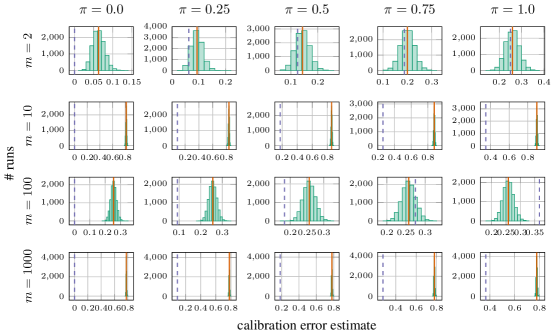
Figure 3: Distribution of $\widehat{\operatorname{ECE}}$ with bins of uniform size, evaluated on $10^{4}$ data sets of 250 labeled predictions that are randomly sampled from generative models with $\alpha=(1,\ldots,1)$ and $\beta=(1/m,\ldots,1/m)$.

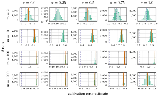
Figure 4: Distribution of $\widehat{\operatorname{ECE}}$ with bins of uniform size, evaluated on $10^{4}$ data sets of 250 labeled predictions that are randomly sampled from generative models with $\alpha=(0.1,\ldots,0.1)$ and $\beta=(1/m,\ldots,1/m)$.

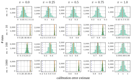
Figure 5: Distribution of $\widehat{\operatorname{ECE}}$ with bins of uniform size, evaluated on $10^{4}$ data sets of 250 labeled predictions that are randomly sampled from generative models with $\alpha=(1,\ldots,1)$ and $\beta=(1,0,\ldots,0)$.

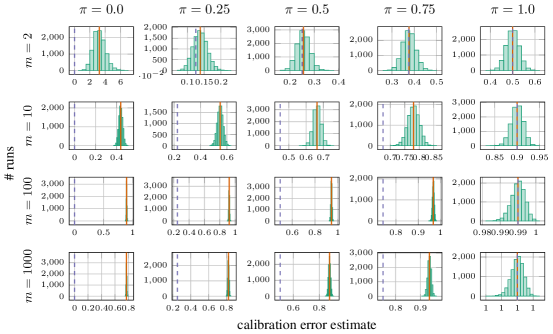
Figure 6: Distribution of $\widehat{\operatorname{ECE}}$ with bins of uniform size, evaluated on $10^{4}$ data sets of 250 labeled predictions that are randomly sampled from generative models with $\alpha=(0.1,\ldots,0.1)$ and $\beta=(1,0,\ldots,0)$.

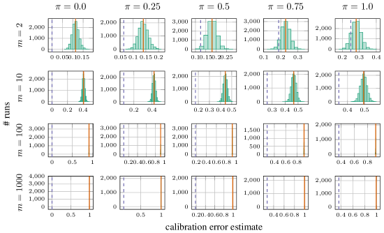
Figure 7: Distribution of $\widehat{\operatorname{ECE}}$ with data-dependent bins, evaluated on $10^{4}$ data sets of 250 labeled predictions that are randomly sampled from generative models with $\alpha=(1,\ldots,1)$ and $\beta=(1/m,\ldots,1/m)$.

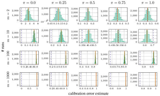
Figure 8: Distribution of $\widehat{\operatorname{ECE}}$ with data-dependent bins, evaluated on $10^{4}$ data sets of 250 labeled predictions that are randomly sampled from generative models with $\alpha=(0.1,\ldots,0.1)$ and $\beta=(1/m,\ldots,1/m)$.

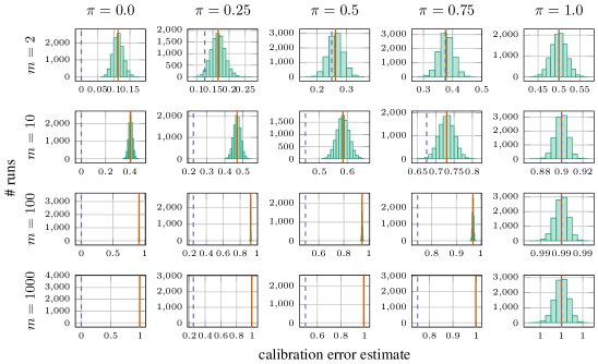
Figure 9: Distribution of $\widehat{\operatorname{ECE}}$ with data-dependent bins, evaluated on $10^{4}$ data sets of 250 labeled predictions that are randomly sampled from generative models with $\alpha=(1,\ldots,1)$ and $\beta=(1,0,\ldots,0)$.

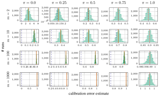
Figure 10: Distribution of $\widehat{\operatorname{ECE}}$ with data-dependent bins, evaluated on $10^{4}$ data sets of 250 labeled predictions that are randomly sampled from generative models with $\alpha=(0.1,\ldots,0.1)$ and $\beta=(1,0,\ldots,0)$.

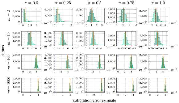
Figure 11: Distribution of $\operatorname{\widehat{SKCE}_{b}}$ with the median heuristic, evaluated on $10^{4}$ data sets of 250 labeled predictions that are randomly sampled from generative models with $\alpha=(1,\ldots,1)$ and $\beta=(1/m,\ldots,1/m)$.

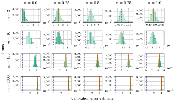
Figure 12: Distribution of $\operatorname{\widehat{SKCE}_{b}}$ with the median heuristic, evaluated on $10^{4}$ data sets of 250 labeled predictions that are randomly sampled from generative models with $\alpha=(0.1,\ldots,0.1)$ and $\beta=(1/m,\ldots,1/m)$.

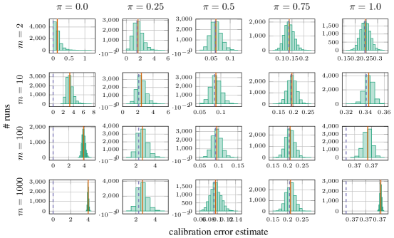
Figure 13: Distribution of $\operatorname{\widehat{SKCE}_{b}}$ with the median heuristic, evaluated on $10^{4}$ data sets of 250 labeled predictions that are randomly sampled from generative models with $\alpha=(1,\ldots,1)$ and $\beta=(1,0,\ldots,0)$.

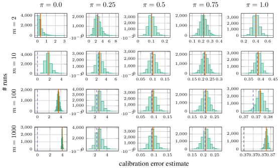
Figure 14: Distribution of $\operatorname{\widehat{SKCE}_{b}}$ with the median heuristic, evaluated on $10^{4}$ data sets of 250 labeled predictions that are randomly sampled from generative models with $\alpha=(0.1,\ldots,0.1)$ and $\beta=(1,0,\ldots,0)$.

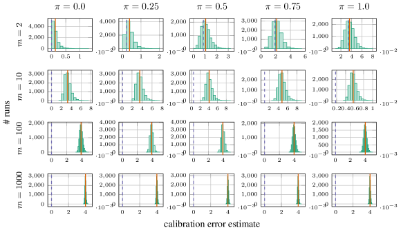
Figure 15: Distribution of $\operatorname{\widehat{SKCE}_{b}}$ with the mean total variation distance, evaluated on $10^{4}$ data sets of 250 labeled predictions that are randomly sampled from generative models with $\alpha=(1,\ldots,1)$ and $\beta=(1/m,\ldots,1/m)$.

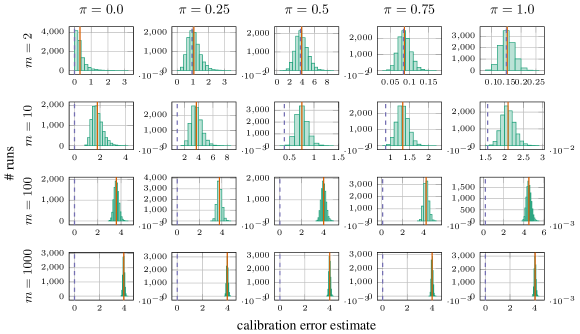
Figure 16: Distribution of $\operatorname{\widehat{SKCE}_{b}}$ with the mean total variation distance, evaluated on $10^{4}$ data sets of 250 labeled predictions that are randomly sampled from generative models with $\alpha=(0.1,\ldots,0.1)$ and $\beta=(1/m,\ldots,1/m)$.

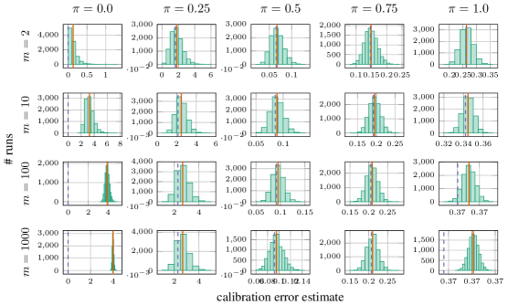
Figure 17: Distribution of $\operatorname{\widehat{SKCE}_{b}}$ with the mean total variation distance, evaluated on $10^{4}$ data sets of 250 labeled predictions that are randomly sampled from generative models with $\alpha=(1,\ldots,1)$ and $\beta=(1,0,\ldots,0)$.

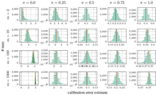
Figure 18: Distribution of $\operatorname{\widehat{SKCE}_{b}}$ with the mean total variation distance, evaluated on $10^{4}$ data sets of 250 labeled predictions that are randomly sampled from generative models with $\alpha=(0.1,\ldots,0.1)$ and $\beta=(1,0,\ldots,0)$.

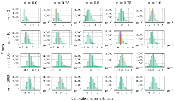
Figure 19: Distribution of $\operatorname{\widehat{SKCE}_{uq}}$ with the median heuristic, evaluated on $10^{4}$ data sets of 250 labeled predictions that are randomly sampled from generative models with $\alpha=(1,\ldots,1)$ and $\beta=(1/m,\ldots,1/m)$.

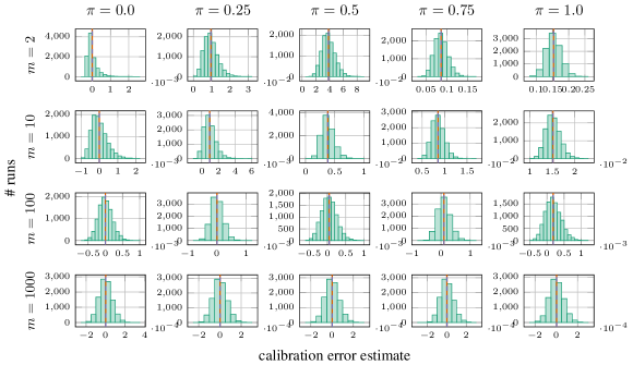
Figure 20: Distribution of $\operatorname{\widehat{SKCE}_{uq}}$ with the median heuristic, evaluated on $10^{4}$ data sets of 250 labeled predictions that are randomly sampled from generative models with $\alpha=(0.1,\ldots,0.1)$ and $\beta=(1/m,\ldots,1/m)$.

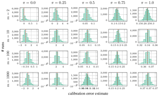
Figure 21: Distribution of $\operatorname{\widehat{SKCE}_{uq}}$ with the median heuristic, evaluated on $10^{4}$ data sets of 250 labeled predictions that are randomly sampled from generative models with $\alpha=(1,\ldots,1)$ and $\beta=(1,0,\ldots,0)$.

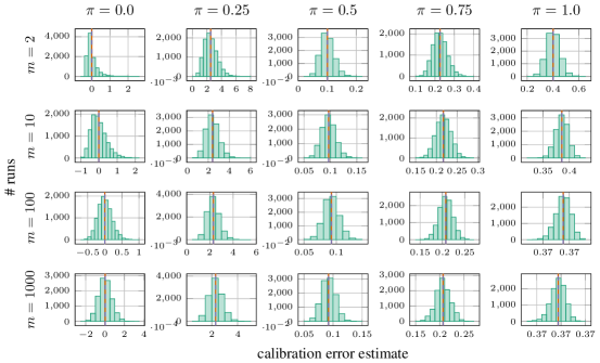
Figure 22: Distribution of $\operatorname{\widehat{SKCE}_{uq}}$ with the median heuristic, evaluated on $10^{4}$ data sets of 250 labeled predictions that are randomly sampled from generative models with $\alpha=(0.1,\ldots,0.1)$ and $\beta=(1,0,\ldots,0)$.

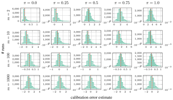
Figure 23: Distribution of $\operatorname{\widehat{SKCE}_{uq}}$ with the mean total variation distance, evaluated on $10^{4}$ data sets of 250 labeled predictions that are randomly sampled from generative models with $\alpha=(1,\ldots,1)$ and $\beta=(1/m,\ldots,1/m)$.

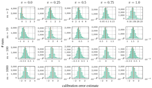
Figure 24: Distribution of $\operatorname{\widehat{SKCE}_{uq}}$ with the mean total variation distance, evaluated on $10^{4}$ data sets of 250 labeled predictions that are randomly sampled from generative models with $\alpha=(0.1,\ldots,0.1)$ and $\beta=(1/m,\ldots,1/m)$.

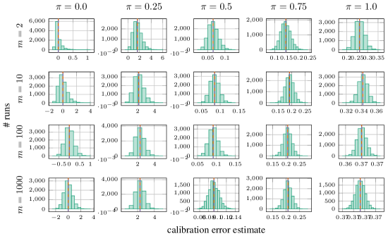
Figure 25: Distribution of $\operatorname{\widehat{SKCE}_{uq}}$ with the mean total variation distance, evaluated on $10^{4}$ data sets of 250 labeled predictions that are randomly sampled from generative models with $\alpha=(1,\ldots,1)$ and $\beta=(1,0,\ldots,0)$.

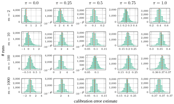
Figure 26: Distribution of $\operatorname{\widehat{SKCE}_{uq}}$ with the mean total variation distance, evaluated on $10^{4}$ data sets of 250 labeled predictions that are randomly sampled from generative models with $\alpha=(0.1,\ldots,0.1)$ and $\beta=(1,0,\ldots,0)$.

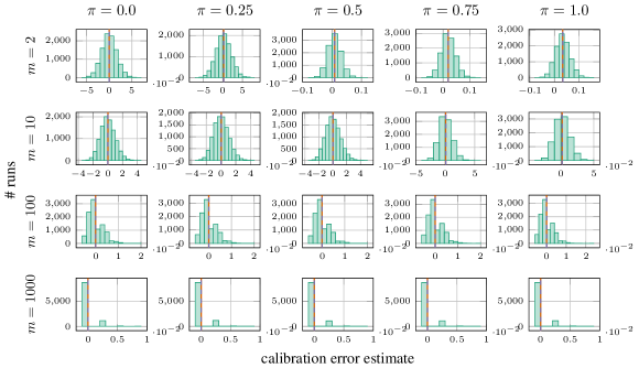
Figure 27: Distribution of $\operatorname{\widehat{SKCE}_{ul}}$ with the median heuristic, evaluated on $10^{4}$ data sets of 250 labeled predictions that are randomly sampled from generative models with $\alpha=(1,\ldots,1)$ and $\beta=(1/m,\ldots,1/m)$.

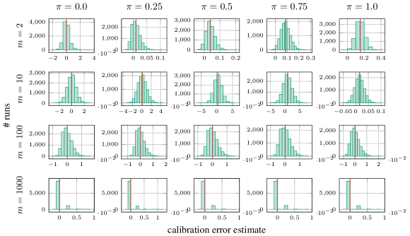
Figure 28: Distribution of $\operatorname{\widehat{SKCE}_{ul}}$ with the median heuristic, evaluated on $10^{4}$ data sets of 250 labeled predictions that are randomly sampled from generative models with $\alpha=(0.1,\ldots,0.1)$ and $\beta=(1/m,\ldots,1/m)$.

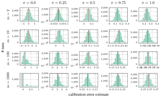
Figure 29: Distribution of $\operatorname{\widehat{SKCE}_{ul}}$ with the median heuristic, evaluated on $10^{4}$ data sets of 250 labeled predictions that are randomly sampled from generative models with $\alpha=(1,\ldots,1)$ and $\beta=(1,0,\ldots,0)$.

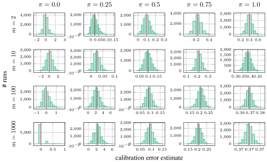
Figure 30: Distribution of $\operatorname{\widehat{SKCE}_{ul}}$ with the median heuristic, evaluated on $10^{4}$ data sets of 250 labeled predictions that are randomly sampled from generative models with $\alpha=(0.1,\ldots,0.1)$ and $\beta=(1,0,\ldots,0)$.

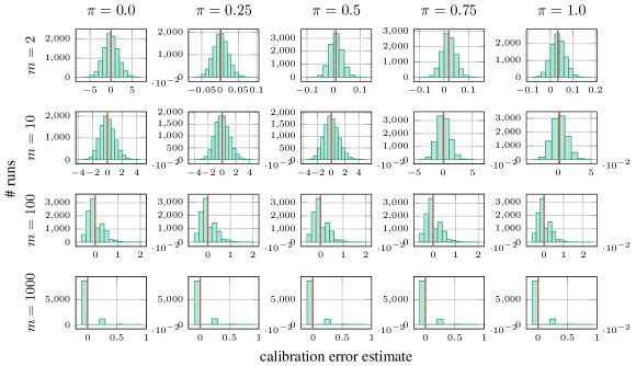
Figure 31: Distribution of $\operatorname{\widehat{SKCE}_{ul}}$ with the mean total variation distance, evaluated on $10^{4}$ data sets of 250 labeled predictions that are randomly sampled from generative models with $\alpha=(1,\ldots,1)$ and $\beta=(1/m,\ldots,1/m)$.

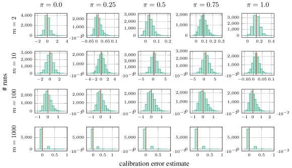
Figure 32: Distribution of $\operatorname{\widehat{SKCE}_{ul}}$ with the mean total variation distance, evaluated on $10^{4}$ data sets of 250 labeled predictions that are randomly sampled from generative models with $\alpha=(0.1,\ldots,0.1)$ and $\beta=(1/m,\ldots,1/m)$.

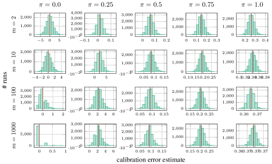
Figure 33: Distribution of $\operatorname{\widehat{SKCE}_{ul}}$ with the mean total variation distance, evaluated on $10^{4}$ data sets of 250 labeled predictions that are randomly sampled from generative models with $\alpha=(1,\ldots,1)$ and $\beta=(1,0,\ldots,0)$.

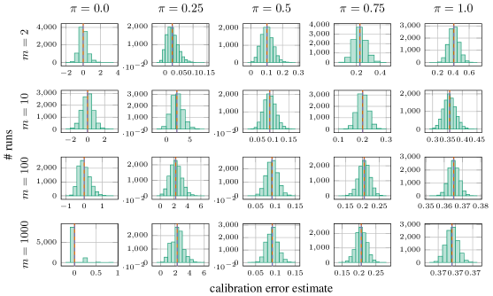
Figure 34: Distribution of $\operatorname{\widehat{SKCE}_{ul}}$ with the mean total variation distance, evaluated on $10^{4}$ data sets of 250 labeled predictions that are randomly sampled from generative models with $\alpha=(0.1,\ldots,0.1)$ and $\beta=(1,0,\ldots,0)$.

J.2.4 Calibration tests: Additional figures

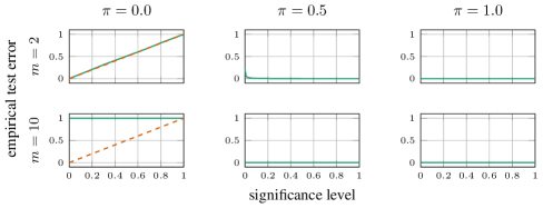
Figure 35: Empirical test error versus significance level for approximations of the p-value with consistency resampling based on $\widehat{\operatorname{ECE}}$ with bins of uniform size, evaluated on $10^{4}$ data sets of 250 labeled predictions that are randomly sampled from generative models with $\alpha=(1,\ldots,1)$ and $\beta=(1/m,\ldots,1/m)$.

Figure 36: Empirical test error versus significance level for approximations of the p-value with consistency resampling based on $\widehat{\operatorname{ECE}}$ with bins of uniform size, evaluated on $10^{4}$ data sets of 250 labeled predictions that are randomly sampled from generative models with $\alpha=(0.1,\ldots,0.1)$ and $\beta=(1/m,\ldots,1/m)$.

Figure 37: Empirical test error versus significance level for approximations of the p-value with consistency resampling based on $\widehat{\operatorname{ECE}}$ with bins of uniform size, evaluated on $10^{4}$ data sets of 250 labeled predictions that are randomly sampled from generative models with $\alpha=(1,\ldots,1)$ and $\beta=(1,0,\ldots,0)$.

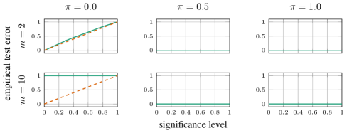
Figure 38: Empirical test error versus significance level for approximations of the p-value with consistency resampling based on $\widehat{\operatorname{ECE}}$ with bins of uniform size, evaluated on $10^{4}$ data sets of 250 labeled predictions that are randomly sampled from generative models with $\alpha=(0.1,\ldots,0.1)$ and $\beta=(1,0,\ldots,0)$.

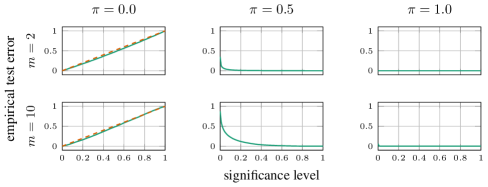
Figure 39: Empirical test error versus significance level for approximations of the p-value with consistency resampling based on $\widehat{\operatorname{ECE}}$ with data-dependent bins, evaluated on $10^{4}$ data sets of 250 labeled predictions that are randomly sampled from generative models with $\alpha=(1,\ldots,1)$ and $\beta=(1/m,\ldots,1/m)$.

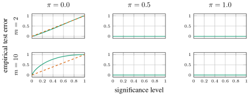
Figure 40: Empirical test error versus significance level for approximations of the p-value with consistency resampling based on $\widehat{\operatorname{ECE}}$ with data-dependent bins, evaluated on $10^{4}$ data sets of 250 labeled predictions that are randomly sampled from generative models with $\alpha=(0.1,\ldots,0.1)$ and $\beta=(1/m,\ldots,1/m)$.

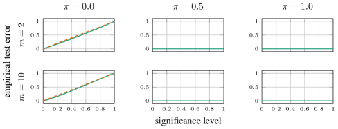
Figure 41: Empirical test error versus significance level for approximations of the p-value with consistency resampling based on $\widehat{\operatorname{ECE}}$ with data-dependent bins, evaluated on $10^{4}$ data sets of 250 labeled predictions that are randomly sampled from generative models with $\alpha=(1,\ldots,1)$ and $\beta=(1,0,\ldots,0)$.

Figure 42: Empirical test error versus significance level for approximations of the p-value with consistency resampling based on $\widehat{\operatorname{ECE}}$ with data-dependent bins, evaluated on $10^{4}$ data sets of 250 labeled predictions that are randomly sampled from generative models with $\alpha=(0.1,\ldots,0.1)$ and $\beta=(1,0,\ldots,0)$.

Figure 43: Empirical test error versus significance level for distribution-free bounds of the p-value based on $\operatorname{\widehat{SKCE}_{b}}$ with the median heuristic, evaluated on $10^{4}$ data sets of 250 labeled predictions that are randomly sampled from generative models with $\alpha=(1,\ldots,1)$ and $\beta=(1/m,\ldots,1/m)$.

Figure 44: Empirical test error versus significance level for distribution-free bounds of the p-value based on $\operatorname{\widehat{SKCE}_{b}}$ with the median heuristic, evaluated on $10^{4}$ data sets of 250 labeled predictions that are randomly sampled from generative models with $\alpha=(0.1,\ldots,0.1)$ and $\beta=(1/m,\ldots,1/m)$.

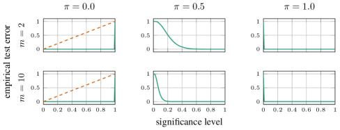
Figure 45: Empirical test error versus significance level for distribution-free bounds of the p-value based on $\operatorname{\widehat{SKCE}_{b}}$ with the median heuristic, evaluated on $10^{4}$ data sets of 250 labeled predictions that are randomly sampled from generative models with $\alpha=(1,\ldots,1)$ and $\beta=(1,0,\ldots,0)$.

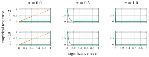
Figure 46: Empirical test error versus significance level for distribution-free bounds of the p-value based on $\operatorname{\widehat{SKCE}_{b}}$ with the median heuristic, evaluated on $10^{4}$ data sets of 250 labeled predictions that are randomly sampled from generative models with $\alpha=(0.1,\ldots,0.1)$ and $\beta=(1,0,\ldots,0)$.

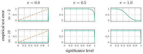
Figure 47: Empirical test error versus significance level for distribution-free bounds of the p-value based on $\operatorname{\widehat{SKCE}_{b}}$ with the mean total variation distance, evaluated on $10^{4}$ data sets of 250 labeled predictions that are randomly sampled from generative models with $\alpha=(1,\ldots,1)$ and $\beta=(1/m,\ldots,1/m)$.

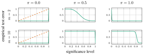
Figure 48: Empirical test error versus significance level for distribution-free bounds of the p-value based on $\operatorname{\widehat{SKCE}_{b}}$ with the mean total variation distance, evaluated on $10^{4}$ data sets of 250 labeled predictions that are randomly sampled from generative models with $\alpha=(0.1,\ldots,0.1)$ and $\beta=(1/m,\ldots,1/m)$.

Figure 49: Empirical test error versus significance level for distribution-free bounds of the p-value based on $\operatorname{\widehat{SKCE}_{b}}$ with the mean total variation distance, evaluated on $10^{4}$ data sets of 250 labeled predictions that are randomly sampled from generative models with $\alpha=(1,\ldots,1)$ and $\beta=(1,0,\ldots,0)$.

Figure 50: Empirical test error versus significance level for distribution-free bounds of the p-value based on $\operatorname{\widehat{SKCE}_{b}}$ with the mean total variation distance, evaluated on $10^{4}$ data sets of 250 labeled predictions that are randomly sampled from generative models with $\alpha=(0.1,\ldots,0.1)$ and $\beta=(1,0,\ldots,0)$.

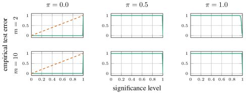
Figure 51: Empirical test error versus significance level for distribution-free bounds of the p-value based on $\operatorname{\widehat{SKCE}_{uq}}$ with the median heuristic, evaluated on $10^{4}$ data sets of 250 labeled predictions that are randomly sampled from generative models with $\alpha=(1,\ldots,1)$ and $\beta=(1/m,\ldots,1/m)$.

Figure 52: Empirical test error versus significance level for distribution-free bounds of the p-value based on $\operatorname{\widehat{SKCE}_{uq}}$ with the median heuristic, evaluated on $10^{4}$ data sets of 250 labeled predictions that are randomly sampled from generative models with $\alpha=(0.1,\ldots,0.1)$ and $\beta=(1/m,\ldots,1/m)$.

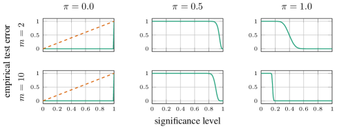
Figure 53: Empirical test error versus significance level for distribution-free bounds of the p-value based on $\operatorname{\widehat{SKCE}_{uq}}$ with the median heuristic, evaluated on $10^{4}$ data sets of 250 labeled predictions that are randomly sampled from generative models with $\alpha=(1,\ldots,1)$ and $\beta=(1,0,\ldots,0)$.

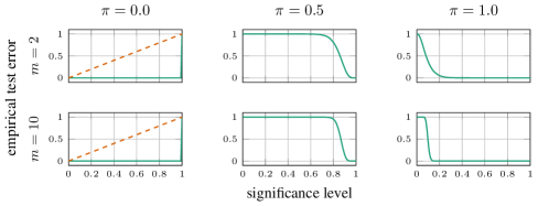
Figure 54: Empirical test error versus significance level for distribution-free bounds of the p-value based on $\operatorname{\widehat{SKCE}_{uq}}$ with the median heuristic, evaluated on $10^{4}$ data sets of 250 labeled predictions that are randomly sampled from generative models with $\alpha=(0.1,\ldots,0.1)$ and $\beta=(1,0,\ldots,0)$.

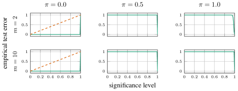
Figure 55: Empirical test error versus significance level for distribution-free bounds of the p-value based on $\operatorname{\widehat{SKCE}_{uq}}$ with the mean total variation distance, evaluated on $10^{4}$ data sets of 250 labeled predictions that are randomly sampled from generative models with $\alpha=(1,\ldots,1)$ and $\beta=(1/m,\ldots,1/m)$.

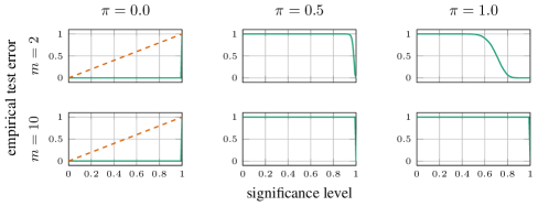
Figure 56: Empirical test error versus significance level for distribution-free bounds of the p-value based on $\operatorname{\widehat{SKCE}_{uq}}$ with the mean total variation distance, evaluated on $10^{4}$ data sets of 250 labeled predictions that are randomly sampled from generative models with $\alpha=(0.1,\ldots,0.1)$ and $\beta=(1/m,\ldots,1/m)$.

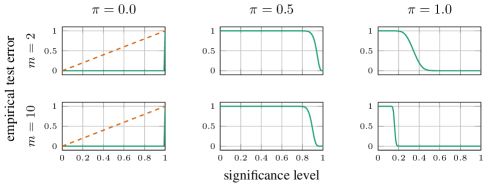
Figure 57: Empirical test error versus significance level for distribution-free bounds of the p-value based on $\operatorname{\widehat{SKCE}_{uq}}$ with the mean total variation distance, evaluated on $10^{4}$ data sets of 250 labeled predictions that are randomly sampled from generative models with $\alpha=(1,\ldots,1)$ and $\beta=(1,0,\ldots,0)$.

Figure 58: Empirical test error versus significance level for distribution-free bounds of the p-value based on $\operatorname{\widehat{SKCE}_{uq}}$ with the mean total variation distance, evaluated on $10^{4}$ data sets of 250 labeled predictions that are randomly sampled from generative models with $\alpha=(0.1,\ldots,0.1)$ and $\beta=(1,0,\ldots,0)$.

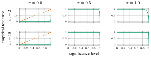
Figure 59: Empirical test error versus significance level for distribution-free bounds of the p-value based on $\operatorname{\widehat{SKCE}_{ul}}$ with the median heuristic, evaluated on $10^{4}$ data sets of 250 labeled predictions that are randomly sampled from generative models with $\alpha=(1,\ldots,1)$ and $\beta=(1/m,\ldots,1/m)$.

Figure 60: Empirical test error versus significance level for distribution-free bounds of the p-value based on $\operatorname{\widehat{SKCE}_{ul}}$ with the median heuristic, evaluated on $10^{4}$ data sets of 250 labeled predictions that are randomly sampled from generative models with $\alpha=(0.1,\ldots,0.1)$ and $\beta=(1/m,\ldots,1/m)$.

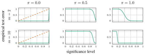
Figure 61: Empirical test error versus significance level for distribution-free bounds of the p-value based on $\operatorname{\widehat{SKCE}_{ul}}$ with the median heuristic, evaluated on $10^{4}$ data sets of 250 labeled predictions that are randomly sampled from generative models with $\alpha=(1,\ldots,1)$ and $\beta=(1,0,\ldots,0)$.

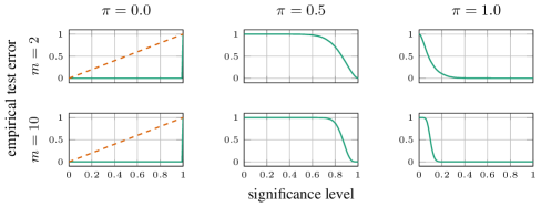
Figure 62: Empirical test error versus significance level for distribution-free bounds of the p-value based on $\operatorname{\widehat{SKCE}_{ul}}$ with the median heuristic, evaluated on $10^{4}$ data sets of 250 labeled predictions that are randomly sampled from generative models with $\alpha=(0.1,\ldots,0.1)$ and $\beta=(1,0,\ldots,0)$.

Figure 63: Empirical test error versus significance level for distribution-free bounds of the p-value based on $\operatorname{\widehat{SKCE}_{ul}}$ with the mean total variation distance, evaluated on $10^{4}$ data sets of 250 labeled predictions that are randomly sampled from generative models with $\alpha=(1,\ldots,1)$ and $\beta=(1/m,\ldots,1/m)$.

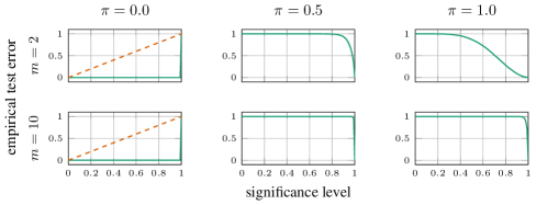
Figure 64: Empirical test error versus significance level for distribution-free bounds of the p-value based on $\operatorname{\widehat{SKCE}_{ul}}$ with the mean total variation distance, evaluated on $10^{4}$ data sets of 250 labeled predictions that are randomly sampled from generative models with $\alpha=(0.1,\ldots,0.1)$ and $\beta=(1/m,\ldots,1/m)$.

Figure 65: Empirical test error versus significance level for distribution-free bounds of the p-value based on $\operatorname{\widehat{SKCE}_{ul}}$ with the mean total variation distance, evaluated on $10^{4}$ data sets of 250 labeled predictions that are randomly sampled from generative models with $\alpha=(1,\ldots,1)$ and $\beta=(1,0,\ldots,0)$.

Figure 66: Empirical test error versus significance level for distribution-free bounds of the p-value based on $\operatorname{\widehat{SKCE}_{ul}}$ with the mean total variation distance, evaluated on $10^{4}$ data sets of 250 labeled predictions that are randomly sampled from generative models with $\alpha=(0.1,\ldots,0.1)$ and $\beta=(1,0,\ldots,0)$.

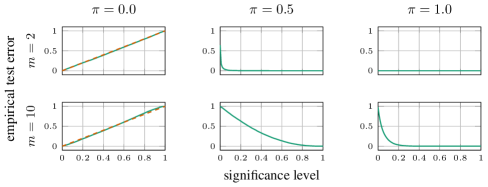
Figure 67: Empirical test error versus significance level for asymptotic approximations of the p-value based on $\operatorname{\widehat{SKCE}_{uq}}$ with the median heuristic, evaluated on $10^{4}$ data sets of 250 labeled predictions that are randomly sampled from generative models with $\alpha=(1,\ldots,1)$ and $\beta=(1/m,\ldots,1/m)$.

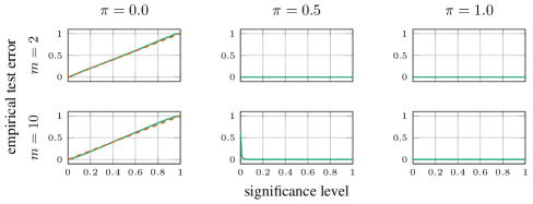
Figure 68: Empirical test error versus significance level for asymptotic approximations of the p-value based on $\operatorname{\widehat{SKCE}_{uq}}$ with the median heuristic, evaluated on $10^{4}$ data sets of 250 labeled predictions that are randomly sampled from generative models with $\alpha=(0.1,\ldots,0.1)$ and $\beta=(1/m,\ldots,1/m)$.

Figure 69: Empirical test error versus significance level for asymptotic approximations of the p-value based on $\operatorname{\widehat{SKCE}_{uq}}$ with the median heuristic, evaluated on $10^{4}$ data sets of 250 labeled predictions that are randomly sampled from generative models with $\alpha=(1,\ldots,1)$ and $\beta=(1,0,\ldots,0)$.

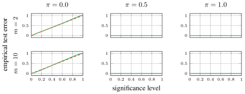
Figure 70: Empirical test error versus significance level for asymptotic approximations of the p-value based on $\operatorname{\widehat{SKCE}_{uq}}$ with the median heuristic, evaluated on $10^{4}$ data sets of 250 labeled predictions that are randomly sampled from generative models with $\alpha=(0.1,\ldots,0.1)$ and $\beta=(1,0,\ldots,0)$.

Figure 71: Empirical test error versus significance level for asymptotic approximations of the p-value based on $\operatorname{\widehat{SKCE}_{uq}}$ with the mean total variation distance, evaluated on $10^{4}$ data sets of 250 labeled predictions that are randomly sampled from generative models with $\alpha=(1,\ldots,1)$ and $\beta=(1/m,\ldots,1/m)$.

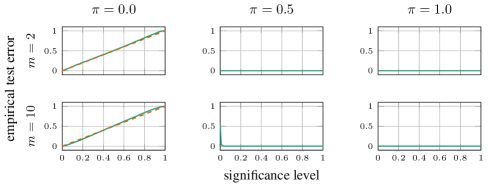
Figure 72: Empirical test error versus significance level for asymptotic approximations of the p-value based on $\operatorname{\widehat{SKCE}_{uq}}$ with the mean total variation distance, evaluated on $10^{4}$ data sets of 250 labeled predictions that are randomly sampled from generative models with $\alpha=(0.1,\ldots,0.1)$ and $\beta=(1/m,\ldots,1/m)$.

Figure 73: Empirical test error versus significance level for asymptotic approximations of the p-value based on $\operatorname{\widehat{SKCE}_{uq}}$ with the mean total variation distance, evaluated on $10^{4}$ data sets of 250 labeled predictions that are randomly sampled from generative models with $\alpha=(1,\ldots,1)$ and $\beta=(1,0,\ldots,0)$.

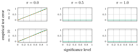
Figure 74: Empirical test error versus significance level for asymptotic approximations of the p-value based on $\operatorname{\widehat{SKCE}_{uq}}$ with the mean total variation distance, evaluated on $10^{4}$ data sets of 250 labeled predictions that are randomly sampled from generative models with $\alpha=(0.1,\ldots,0.1)$ and $\beta=(1,0,\ldots,0)$.

Figure 75: Empirical test error versus significance level for asymptotic approximations of the p-value based on $\operatorname{\widehat{SKCE}_{ul}}$ with the median heuristic, evaluated on $10^{4}$ data sets of 250 labeled predictions that are randomly sampled from generative models with $\alpha=(1,\ldots,1)$ and $\beta=(1/m,\ldots,1/m)$.

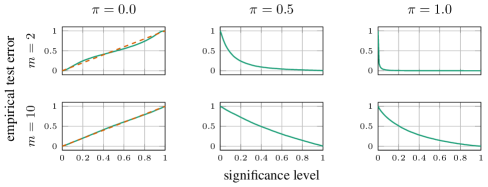
Figure 76: Empirical test error versus significance level for asymptotic approximations of the p-value based on $\operatorname{\widehat{SKCE}_{ul}}$ with the median heuristic, evaluated on $10^{4}$ data sets of 250 labeled predictions that are randomly sampled from generative models with $\alpha=(0.1,\ldots,0.1)$ and $\beta=(1/m,\ldots,1/m)$.

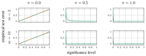
Figure 77: Empirical test error versus significance level for asymptotic approximations of the p-value based on $\operatorname{\widehat{SKCE}_{ul}}$ with the median heuristic, evaluated on $10^{4}$ data sets of 250 labeled predictions that are randomly sampled from generative models with $\alpha=(1,\ldots,1)$ and $\beta=(1,0,\ldots,0)$.

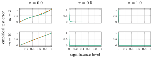
Figure 78: Empirical test error versus significance level for asymptotic approximations of the p-value based on $\operatorname{\widehat{SKCE}_{ul}}$ with the median heuristic, evaluated on $10^{4}$ data sets of 250 labeled predictions that are randomly sampled from generative models with $\alpha=(0.1,\ldots,0.1)$ and $\beta=(1,0,\ldots,0)$.

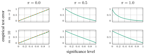
Figure 79: Empirical test error versus significance level for asymptotic approximations of the p-value based on $\operatorname{\widehat{SKCE}_{ul}}$ with the mean total variation distance, evaluated on $10^{4}$ data sets of 250 labeled predictions that are randomly sampled from generative models with $\alpha=(1,\ldots,1)$ and $\beta=(1/m,\ldots,1/m)$.

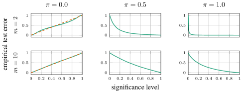
Figure 80: Empirical test error versus significance level for asymptotic approximations of the p-value based on $\operatorname{\widehat{SKCE}_{ul}}$ with the mean total variation distance, evaluated on $10^{4}$ data sets of 250 labeled predictions that are randomly sampled from generative models with $\alpha=(0.1,\ldots,0.1)$ and $\beta=(1/m,\ldots,1/m)$.

Figure 81: Empirical test error versus significance level for asymptotic approximations of the p-value based on $\operatorname{\widehat{SKCE}_{ul}}$ with the mean total variation distance, evaluated on $10^{4}$ data sets of 250 labeled predictions that are randomly sampled from generative models with $\alpha=(1,\ldots,1)$ and $\beta=(1,0,\ldots,0)$.

Figure 82: Empirical test error versus significance level for asymptotic approximations of the p-value based on $\operatorname{\widehat{SKCE}_{ul}}$ with the mean total variation distance, evaluated on $10^{4}$ data sets of 250 labeled predictions that are randomly sampled from generative models with $\alpha=(0.1,\ldots,0.1)$ and $\beta=(1,0,\ldots,0)$.

J.3 Modern neural networks

In the main experiments of our paper discussed in Section J.2 we focus on an experimental confirmation of the derived theoretical properties of the kernel-based estimators and their comparison with the commonly used $\operatorname{ECE}$. In contrast to Guo et al. (2017), neither the study of the calibration of different neural network architectures nor the re-calibration of uncalibrated models are the main goal of our paper. The calibration measures that we consider only depend on the predictions and the true labels, not on how these predictions are computed. We therefore believe that directly specifying the predictions in a “controlled way” results in a cleaner and more informative numerical evaluation.

That being said, we recognize that this approach might result in an unnecessary disconnect between the results of the paper and a practical use case. We therefore conduct additional evaluations with different modern neural networks as well. We consider pretrained ResNet, DenseNet, VGGNet, GoogLeNet, MobileNet, and Inception neural networks (Phan, 2019) for the classification of the CIFAR-10 image data set (Krizhevsky, 2009). The CIFAR-10 data set is a labeled data set of $32\times 32$ colour images and consists of 50000 training and 10000 test images in 10 classes. The calibration of the neural network models is estimated from their predictions on the CIFAR-10 test data set. We use the same calibration error estimators and p-value approximations as for the generative models above; however, the minimum number of samples per bin in the data-dependent binning scheme of the $\operatorname{ECE}$ estimator is increased to 100 to account for the increased number of data samples.

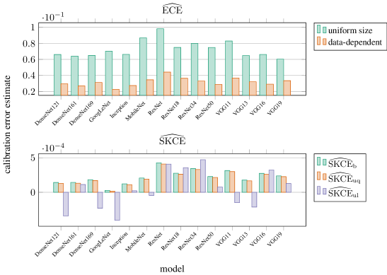
Figure 83: Calibration error estimates of modern neural networks for classification of the CIFAR-10 image data set.

The computed calibration error estimates are shown in Fig. 83. As we argue in our paper, the raw calibration estimates are not interpretable and can be misleading. The results in Fig. 83 endorse this opinion. The estimators rank the models in different order (also the two estimators of the $\operatorname{ECE}$), and it is completely unclear if the observed calibration error estimates (in the order of $10^{-2}$ and $10^{-4}$!) actually indicate that the neural network models are not calibrated.

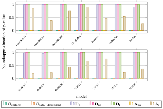
Figure 84: Bounds and approximations of the p-value of modern neural networks for classification of the CIFAR-10 image data set for different calibration error estimators, assuming the models are calibrated.

Hence to obtain an interpretable measure, we consider different bounds and approximations of the p-value for the calibration error estimators, assuming the models are calibrated. More concretely, we estimate the p-value by consistency resampling of the standard ($\mathbf{C}_{\mathrm{uniform}}$) and the data-dependent ($\mathbf{C}_{\mathrm{data-dependent}}$) estimator of the $\operatorname{ECE}$, evaluate the distribution-free bounds of the p-value for the estimators $\operatorname{\widehat{SKCE}_{b}}$ ($\mathbf{D}_{\mathrm{b}}$), $\operatorname{\widehat{SKCE}_{uq}}$ ($\mathbf{D}_{\mathrm{uq}}$), and $\operatorname{\widehat{SKCE}_{ul}}$ ($\mathbf{D}_{\mathrm{l}}$) of the $\operatorname{SKCE}$, and approximate the p-value using the asymptotic distribution of the estimators $\operatorname{\widehat{SKCE}_{uq}}$ ($\mathbf{A}_{\mathrm{uq}}$) and $\operatorname{\widehat{SKCE}_{ul}}$ ($\mathbf{A}_{\mathrm{l}}$). The results are shown in Fig. 84.

The approximations obtained by consistency resampling are always zero. However, since our controlled experiments with the generative models showed that consistency resampling might underestimate the p-value of calibrated models on average, these approximations could be misleading. On the contrary, the bounds and approximations of the p-value for the estimators of the $\operatorname{SKCE}$ are theoretically well-founded. In our experiments with the generative models, the asymptotic distribution of the estimator $\operatorname{\widehat{SKCE}_{uq}}$ seemed to allow to approximate the p-value quite accurately on average and yielded very powerful tests. For all studied neural network models these p-value approximations are zero, and hence for all models we would always reject the null hypothesis of calibration. The p-value approximations based on the asymptotic distribution of the estimator $\operatorname{\widehat{SKCE}_{ul}}$ vary between around $0.18$ for the ResNet18 and $0.91$ for the GoogLeNet model. The higher p-value approximations correspond to the increased empirical test errors with the uncalibrated generative models compared to the tests based on the asymptotic distribution of the estimator $\operatorname{\widehat{SKCE}_{uq}}$. Most distribution-free bounds of the p-value are between 0.99 and 1, indicating again that these bounds are quite loose.

All in all, the evaluations of the modern neural networks seem to match the theoretical expectations and are consistent with the results we obtained in the experiments with the generative models. Moreover, the p-value approximations of zero are consistent with Guo et al. (2017)’s finding that modern neural networks are often not calibrated.

J.4 Computational time

The computational time, although dependent on our Julia implementation and the hardware used, might provide some insights to the interested reader in addition to the algorithmic complexity. However, in our opinion, a fair comparison of the proposed calibration error estimators should take into account the error of the calibration error estimation, similar to work precision diagrams for numerical differential equation solvers.

A simple comparison of the computational time for the calibration error estimators used in the experiments with the generative models in Section J.2 on our computer (3.6 GHz) shows the expected scaling of the computational time with increasing number of samples. As Fig. 85 shows, even for 1000 samples and 1000 classes the estimators $\operatorname{\widehat{SKCE}_{b}}$ and $\operatorname{\widehat{SKCE}_{uq}}$ with the median heuristic can be evaluated in around 0.1 seconds.

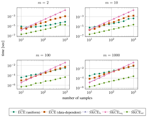
Figure 85: Computational time for the evaluation of calibration error estimators on data sets with different number of classes versus number of data samples.

References

- Arcones and Giné (1992) M. A. Arcones and E. Giné. On the bootstrap of and statistics. The Annals of Statistics, 20(2):655–674, 1992.
- Aronszajn (1950) N. Aronszajn. Theory of reproducing kernels. Transactions of the American Mathematical Society, 68(3):337–337, 3 1950.
- Bartlett and Mendelson (2002) P. L. Bartlett and S. Mendelson. Rademacher and Gaussian complexities: Risk bounds and structural results. Journal of Machine Learning Research, 3:463–482, 2002.
- Berlinet and Thomas-Agnan (2004) A. Berlinet and C. Thomas-Agnan. Reproducing Kernel Hilbert Spaces in Probability and Statistics. Springer US, 2004.
- Bröcker (2009) J. Bröcker. Reliability, sufficiency, and the decomposition of proper scores. Quarterly Journal of the Royal Meteorological Society, 135(643):1512–1519, 7 2009.
- Bröcker (2011) J. Bröcker. Estimating reliability and resolution of probability forecasts through decomposition of the empirical score. Climate Dynamics, 39(3–4):655–667, 2011.
- Bröcker and Smith (2007) J. Bröcker and L. A. Smith. Increasing the reliability of reliability diagrams. Weather and Forecasting, 22(3):651–661, 6 2007.
- Caponnetto et al. (2008) A. Caponnetto, C. A. Micchelli, M. Pontil, and Y. Ying. Universal multi-task kernels. Journal of Machine Learning Research, 9:1615–1646, 6 2008.
- Carmeli et al. (2010) C. Carmeli, E. De Vito, A. Toigo, and V. Umanità. Vector valued reproducing kernel Hilbert spaces and universality. Analysis and Applications, 08(01):19–61, 01 2010.
- Christmann and Steinwart (2008) A. Christmann and I. Steinwart. Support Vector Machines. Information Science and Statistics. Springer New York, 2008.
- DeGroot and Fienberg (1983) M. H. DeGroot and S. E. Fienberg. The comparison and evaluation of forecasters. The Statistician, 32(1/2):12, 3 1983.
- Ferro and Fricker (2012) C. A. T. Ferro and T. E. Fricker. A bias-corrected decomposition of the Brier score. Quarterly Journal of the Royal Meteorological Society, 138(668):1954–1960, 2012.
- Gretton et al. (2012) A. Gretton, K. M. Borgwardt, M. J. Rasch, B. Schölkopf, and A. Smola. A kernel two-sample test. Journal of Machine Learning Research, 13:723–773, 3 2012.
- Guo et al. (2017) C. Guo, G. Pleiss, Y. Sun, and K. Q. Weinberger. On calibration of modern neural networks. In Proceedings of the 34th International Conference on Machine Learning, volume 70 of Proceedings of Machine Learning Research, pages 1321–1330, 2017.
- Hoeffding (1948) W. Hoeffding. A class of statistics with asymptotically normal distribution. The Annals of Mathematical Statistics, 19(3):293–325, 9 1948.
- Hoeffding (1963) W. Hoeffding. Probability inequalities for sums of bounded random variables. Journal of the American Statistical Association, 58(301):13–30, 1963.
- Kiureghian and Ditlevsen (2009) A. D. Kiureghian and O. Ditlevsen. Aleatory or epistemic? Does it matter? Structural Safety, 31(2):105–112, 3 2009.
- Krizhevsky (2009) A. Krizhevsky. Learning multiple layers of features from tiny images. 2009.
- Kumar et al. (2018) A. Kumar, S. Sarawagi, and U. Jain. Trainable calibration measures for neural networks from kernel mean embeddings. In Proceedings of the 35th International Conference on Machine Learning, volume 80 of Proceedings of Machine Learning Research, pages 2805–2814, 2018.
- Kumar et al. (2019) A. Kumar, P. Liang, and T. Ma. Verified uncertainty calibration. In Advances in Neural Information Processing Systems 32. 2019.
- Micchelli and Pontil (2005) C. A. Micchelli and M. Pontil. On learning vector-valued functions. Neural Computation, 17(1):177–204, 2005.
- Murphy and Winkler (1977) A. H. Murphy and R. L. Winkler. Reliability of subjective probability forecasts of precipitation and temperature. Applied Statistics, 26(1):41, 1977.
- Naeini et al. (2015) M. P. Naeini, G. Cooper, and M. Hauskrecht. Obtaining well calibrated probabilities using Bayesian binning. In Twenty-Ninth AAAI Conference on Artificial Intelligence, 2015.
- Pastell (2017) M. Pastell. Weave.jl: Scientific reports using Julia. The Journal of Open Source Software, 2(11):204, Mar. 2017.
- Phan (2019) H. Phan. PyTorch-CIFAR10, 2019. URL https://github.com/huyvnphan/PyTorch-CIFAR10/.
- Rudin (1986) W. Rudin. Real and complex analysis. McGraw-Hill, New York, 3 edition, 1986.
- Serfling (1980) R. J. Serfling, editor. Approximation Theorems of Mathematical Statistics. John Wiley & Sons, Inc., 11 1980.
- Vaicenavicius et al. (2019) J. Vaicenavicius, D. Widmann, C. Andersson, F. Lindsten, J. Roll, and T. B. Schön. Evaluating model calibration in classification. In Proceedings of Machine Learning Research, volume 89 of Proceedings of Machine Learning Research, pages 3459–3467, 2019.
- van der Vaart (1998) A. W. van der Vaart. Asymptotic Statistics. Cambridge University Press, 1998.
- van der Vaart and Wellner (1996) A. W. van der Vaart and J. A. Wellner. Weak Convergence and Empirical Processes. Springer New York, 1996.
- Widmann (2019a) D. Widmann. devmotion/CalibrationErrors.jl: v0.1.0, Sept. 2019a. URL https://doi.org/10.5281/zenodo.3457945.
- Widmann (2019b) D. Widmann. devmotion/CalibrationTests.jl: v0.1.0, Oct. 2019b. URL https://doi.org/10.5281/zenodo.3514933.
- Widmann (2019c) D. Widmann. devmotion/ConsistencyResampling.jl: v0.2.0, May 2019c. URL https://doi.org/10.5281/zenodo.3232854.
- Zadrozny and Elkan (2002) B. Zadrozny and C. Elkan. Transforming classifier scores into accurate multiclass probability estimates. In Proceedings of the eighth ACM SIGKDD international conference on Knowledge discovery and data mining - KDD. ACM Press, 2002.