Ground state mass in short lattices by controlling overconfidence and bias in Bayesian fits

Abstract

We investigate the seemingly ill-defined problem of extracting a ground-state mass from a lattice simulation where the extent of the lattice is not long enough to project out the ground-state properly. We regulate the problem using a Bayesian method. We show that controlling meta-parameters (overconfidence) can allow the data to overcome the input priors (bias). We can write the method as a black-box technique which allows extraction of a ground-state mass, even on a relatively short lattice.

1 Introduction

The numerical extraction of physically relevant quantities from simulations of lattice gauge theories typically involve fitting. The paradigmatic statistical problem is to extract the masses from the measurement of a correlator using the fitting formula

$$C(t)=\sum_{i=0}^{\infty}A_{i}\cosh\left[m_{i}\left(\frac{N}{2}-t\right)\right],$$ (1)

where we assume an ordering $m_{0}<m_{1}<m_{2}\cdots$, and the Euclidean time $t$ runs over a finite set of integers, $0\leq t<N$, and $N$ is the lattice extent in the direction of Euclidean time. The infinite number of parameters is effectively truncated because all the terms with $1/m_{i}\leq 1$ can be absorbed into a single mass $m_{M}$ and coefficient $A_{M}$, so that the sum in eq. (1) can be taken to run only over $M$ states. We will examine the case where periodic boundary conditions are applied, although other boundary conditions can be dealt with by a straightforward extension of the analysis we present.

In the usual fitting method one strives to take $N\gg 1/(m_{1}-m_{0})$. In that case there is a long interval of $t>T$ where one term of the fit suffices. This is usually monitored by computing local masses, $m_{\rm loc}$, which are defined as the solution of the equation

$$\dfrac{\cosh[m_{\rm loc}(t-\frac{N}{2})]}{\cosh[m_{\rm loc}(t-1-\frac{N}{2})]}=\dfrac{C(t)}{C(t-1)},$$ (2)

where the correlation functions on the right are measured inputs. For those $t$ where $m_{\rm loc}$ is constant and independent of $t$, the ground state dominates and the value of $m_{\rm loc}$ is an estimate of $m_{0}$. It is clear that very close to $t=N/2$ and $t=0$, the expression for $C(t)$ in eq. (1) cannot be dominated by the $i=0$ term. As a result, the plateau in $m_{\rm loc}(t)$ that we would like to observe cannot be close to either end. So one must search for $N\gg T\gg 0$, which usually implies that simulations must be performed with large $N$.

Some time ago a Bayesian method was introduced [1] which did not search for $T$. With sufficient control over the method, one could think of extracting the ground state mass even when the condition $N\gg 1/(m_{1}-m_{0})$ is violated, and $m_{\rm loc}$ is not constant. Since the CPU cost for a simulation grows a little faster than linearly in $N$ (every other parameter being fixed), it would be useful to understand the fitting process well enough to be able to reduce $N$ with confidence. In a recent study of hadron masses extracted from QCD simulations of two flavours of light staggered quarks, we came across one such case.

In this paper we examine the process of Bayesian fitting to decide between various ways of treating meta-parameters. Although the process we finally use, successfully, has been used earlier qualitatively [2, 3], there has been no quantitative statement before. In fact, radically different treatments of meta-parameters have been used in lattice gauge theory [4]. So we feel it is important to set down this method as we have used it.

2 Understanding the method

2.1 A simple model

Perhaps the simplest problem of statistical inference is the extraction of the probability that a tossed coin will land heads up. The frequentist answer is to observe tosses of the coin $N$ times. If the number of times this lands heads up is $H$, then the frequentist answer is

$$p=\frac{H}{N}\left[1+{\cal O}\left(\frac{1}{\sqrt{N}}\right)\right].$$ (3)

Understanding the error term is the beginning of a sophisticated analysis [5], which is common background knowledge today for physicists.

A very small number of experiments, $N$, may by chance yield extreme values of $p$ such as 0 or 1. If one analyzes the error terms seriously then one will assign large errors to these extreme values. However, it is possible to regulate these extreme values by doing a Bayesian analysis instead.

A Bayesian analysis of the same experiment would begin by noting that one could improve the method of inference by bringing our prior knowledge into the analysis [2]. Since all of us have observed tosses of coins before, we should take this prior knowledge into account. Call $p_{0}$ our prior knowledge of the probability. This comes from some previous observation which we may or may not have been scrupulous about recording. We can quantify the depth of our prior knowledge by a number $N_{0}$. The quantity $N_{0}$ has no experimental significance at all, since we have never recorded any previous measurements, and therefore, corresponds to what we may call meta-parameters. Quantities such as these are also sometimes called nuisance parameters, since they are not values of parameters we are interested in extracting. Note also, that the meta-parameters are necessary in order to combine two different experiments. In that case $N_{0}$ is simply the number of coin tosses made in the first experiment. An effective prior count of heads is $H_{0}=p_{0}N_{0}$. Note that the choices of $p_{0}$ and $N_{0}$ are completely arbitrary.

The experiment adds to our knowledge, so the result should give us

$$p=\frac{H_{0}+H}{N_{0}+N}$$ (4)

To analyze how rapidly the experiment changes our prior knowledge, we first note that the prior leads us to expect that the result of the experiment should be $E_{0}[H]=Np_{0}$ heads. Suppose that the prior knowledge is very weighty, i.e., $N_{0}\gg N$. Then one may write

$$p=p_{0}+\frac{H-E_{0}[H]}{N_{0}}\left[1-\frac{N}{N_{0}}+\frac{N^{2}}{N_{0}^{2}}+\cdots\right],$$ (5)

so, in this case, the effect of the experiment shifts our experience only slightly. If, on the other hand, our previous experience is slight, so that $N_{0}\ll N$, then

$$p=\frac{H}{N}+\left(\frac{E_{0}[H]-H}{N}\right)\,\left(\frac{N_{0}}{N}\right)\left[1-\frac{N_{0}}{N}+\frac{N_{0}^{2}}{N^{2}}+\cdots\right].$$ (6)

In this case, our previous experience adds mildly to the results of the experiment. The leading term is the frequentist result, but note that the subleading term starts as $1/N^{2}$, instead of $1/N^{3/2}$. In the special case $H=0$, which needed regulation, the leading result is not $p=0$, but $p=p_{0}(N_{0}/N)^{2}$.

An instructive way to understand this is to define $p_{1}=H/N$ and $n=N/N_{0}$. Then the Bayesian formula becomes

$$p=p_{1}+\frac{p_{0}-p_{1}}{1+n}.$$ (7)

The cross over from the region where $n$ is small and eq. (5) holds, to that where $n$ is large and eq. (6) holds becomes clear. The region $n\simeq 1$ is the region of cross over. The Bayesian point of view is often accused of introducing a bias in the experiment in the form of a value for $p_{0}$. This is clearly true, and, to the Bayesian, a feature and not a bug. However, it is clear from the expression in eq. (7) that the problem of bias lies essentially in the choice of $N_{0}$, i.e., in deciding the relative weights given to the prior and the experiment. In order to pin down this notion, we may say that bias (through prior assumptions for physical parameters) is not as important as the degree of overconfidence (through inappropriate choice of meta-parameters).

This discussion can be phrased in the language of fitting parameters to the results of an experiment. This closely parallels a discussion in [3]. Use the convention that heads are recorded as 1 and tails as 0. The experiment generates a series of 0s and 1s, ${\cal E}=\{x_{i}|1\leq i\leq N,x_{i}\in\{0,1\}\}$. Clearly

$$H=\sum_{i}^{N}x_{i}.$$ (8)

The probability distribution from which the $x$s are drawn is

$$B(x_{i}|p) = p^{x_{i}}(1-p)^{1-x_{i}},\qquad{\rm and}$$ (9)

$$P({\cal E}|p) = \prod_{i=1}^{N}B(x_{i}|p)=p^{H}(1-p)^{N-H},$$

since the successive tosses are independent. Note that $p$ is assumed to be given. The expected value of $x$ is $E[x]=p$. The variance is $V[x]=p(1-p)$. The frequentist method of extracting the parameter $p$ form the data $\cal E$ would be to maximize $\log P({\cal E}|p)$. This gives the result $p=H/N$.

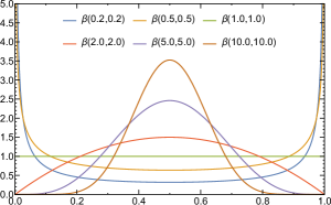
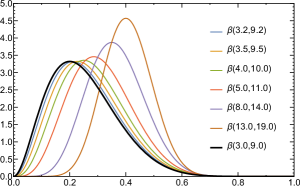
Figure 1: Several prior distributions (upper panel), all with $p_{0}=1/2$ and different $N_{0}$. The x-axis is $p$ and the y-axis is the probability distribution. With increasing $N_{0}$ the prior distribution is narrower. The corresponding posterior distributions (lower panel), with $H=3$ and $N=12$ so that $p_{1}=1/4$. For small $N_{0}$, the posterior distributions $P(p|{\cal E})$ are close to the thick black curve, which is $P({\cal E}|p)$, i.e., the likelihood function.

The Bayesian approach is to find the probability distribution of $p$ given $\cal E$. By Bayes’ theorem, one has

$$P(p|{\cal E})\propto P({\cal E}|p)\,{\rm Pr\/}(p),$$ (10)

where ${\rm Pr\/}(p)$ is the prior distribution of $p$. There are no rules for choosing this distribution, and convenience is the guiding principle. In this example we choose the prior distribution in a form that the posterior distribution, i.e., $P(p|{\cal E})$ is of the same form. This is achieved by the beta distribution,

$${\rm Pr\/}(p)=\beta(p,a,b)=\frac{\Gamma(a+b)}{\Gamma(a)\,\Gamma(b)}p^{a-1}(1-p)^{b-1}.$$ (11)

One has $E[p]=a/(a+b)$ and $V[p]=a(a+1)/(a+b)/(a+b+1)$. The value of $E[p]$ shows that one should make the identification $a=H_{0}$ and $b=N_{0}-H_{0}$. After the experiment, the posterior distribution of $p$ is

$$P(p|{\cal E})=\frac{\Gamma(a+b+N)}{\Gamma(a+H)\,\Gamma(b+N-H)}\times$$ (12)

$$p^{a+H-1}(1-p)^{b+N-H-1}.$$

The expectation value of $p$ in this distribution is exactly the Bayesian result given in eq. (4). As a result, maximizing $\log P(p|{\cal E})$ gives the Bayesian result. The interpretation of this is exactly what we discussed without writing the probability formulae.

An example is shown in Figure 1 with $H=3$ and $N=12$, which means the frequentist result is $p_{1}=1/4$. Different Bayesian priors with $p_{0}=1/2$ are shown for different $N_{0}$. With increasing $N_{0}$ the prior distribution of $p$ is narrower. The Bayesian posterior distributions are also shown. When $N_{0}$ is large, the experimental evidence does not shift the expectation value of $p$, although the distribution changes significantly. As $N_{0}$ becomes small the distributions tend to a limit shown with a thick black line. This limit is equivalent to the frequentist result. For $N_{0}=1$ the expectation value of $p$ is well within the width of the frequentist distribution of $p$. This is compatible with the estimate that the error in $p_{1}$ is of order $1/\sqrt{N}\simeq 0.3$, whereas the bias due to the Bayesian prior is multiplied by $N_{0}/N\simeq 0.1$.

A generalizable lesson is that choosing an inappropriate prior, $p_{0}$ need not be a problem. As long as too much reliance is not placed on the prior (i.e., $N_{0}$ is chosen small enough), the data can lead to the empirically supported probability of heads. In other words, bias is not a problem if overconfidence is avoided.

2.2 Application to fitting

The simplest problems of fitting parameters arise with the so-called linear models, where one has a set of data $C_{i}$ (with $1\leq i\leq N$) which are to be fitted to parameters $p_{\alpha}$ (with $1\leq\alpha\leq P$). The model to be used is $C_{i}=K_{i\alpha}p_{\alpha}$ where the coefficient matrix elements $K_{i\alpha}$ are known. We will collect $C_{i}$ into a vector $C$ and $p_{\alpha}$ into a vector $p$. The simplest example is fitting a straight line to $N$ measurements of data. In this case $P=2$, with $p_{1}$ being possibly the intercept and $p_{2}$ the slope. Then $K_{i1}=1$ for all $i$ and $K_{12}=t_{i}$ where $t_{1}$ is the value of the independent variable at which $C_{i}$ is measured.

If the covariance matrix of the measurements is $\Sigma$, then the usual frequentist procedure [6] is to maximize the probability that the parameters describe the data,

$$P(C|p)\propto{\rm e}^{-\chi^{2}/2},\qquad{\rm where}$$ (13)

$$\chi^{2}=\Delta^{T}\Sigma^{-1}\Delta,\qquad\Delta=C-Kp.$$

Maximizing the posterior probability is the same as minimizing $\chi^{2}$. A Bayesian extension is to maximize the prior probability

$$P(p|C)\propto P(C|p){\rm Pr\/}(p).$$ (14)

Note the similarity to eq. (10).

In the general case, two models for the prior probability distribution are widely used. One corresponding to the Maximum Entropy Method (MEM) is

$${\rm Pr\/}(p)\propto\exp\left(\gamma\sum_{\alpha=1}^{P}\left[p_{\alpha}-p_{\alpha}^{0}-p_{\alpha}\log\left(\frac{p_{\alpha}}{p_{\alpha}^{0}}\right)\right]\right).$$ (15)

The parameter $\gamma$ is the single meta-parameter. The larger it is, the narrower is the prior distribution. So large values of $\gamma$ correspond to overconfidence. The other model is used in the Method of Constrained Fitting (MCF),

$${\rm Pr\/}(p)\propto\prod_{\alpha=1}^{P}\exp\left(-\frac{(p_{\alpha}-p_{\alpha}^{0})^{2}}{2(\sigma_{\alpha}^{0})^{2}}\right).$$ (16)

Here there are multiple meta-parameters $\sigma_{\alpha}^{0}$. The smaller they are, the narrower is the prior distribution. So small values of $\sigma_{\alpha}^{0}$ correspond to overconfidence. In view of the discussion in the preceding subsection, we will dial down the overconfidence by taking the limit of the results when $\gamma\to 0$ or $\sigma_{\alpha}^{0}\to\infty$. We will see later that stability against changes in the values of these meta-parameters sets in quickly, so that the limit is not hard to take. Since the meta-parameters appear only in the prior probability in eq. (14), exactly the same process can be used when the parameters appear non-linearly in the fitting function.

2.3 Application to lattice correlators

It seems reasonable to argue that Bayesian methods work when the posterior is not sensitively dependent on priors, as we saw in the toy model before. This has an effect on the kind of problems which lattice gauge theory can be used for.

The analytic continuation of thermal (Euclidean) correlators to (Minkowski) real-time involves an integral relation formally written as

$$C(t)=\int_{0}^{\infty}d\omega K(\omega,t)\rho(\omega),$$ (17)

where $C(t)$ are the measured values of the correlator at $0\leq t<N_{t}/2$, and $K(\omega,t)$ is a known kernel [7]. Clearly, the extraction of the function $\rho(\omega)$ is a pathologically under-constrained problem if one has no prior knowledge of its form.

Assuming zero knowledge, one may discretize the integral into a Riemann sum over a set $\{\omega_{i}|1\leq i\leq M\}$, and write $K_{i}(t)=K(\omega_{i},t)$ and $\rho_{i}=(\omega_{i}-\omega_{i-1})\rho(\omega_{i})$ choosing $\omega_{0}=0$. Then this becomes a problem of fitting a hyperplane through a set of data:

$$C(t)=\sum_{i=1}^{M}\rho_{i}K_{i}(t).$$ (18)

The ordered set $(K_{1}(t),K_{2}(t)\cdots,K_{M}(t),C(t))$ can be thought of as the coordinate directions in this $M+1$-dimensional space and $\rho_{i}$ are the slopes of the hyperplane which we want to fit. There are only $N_{t}/2+1$ independent pieces of data. When $M>N_{t}/2+1$, none of the $\rho_{i}$ are constrained. Taking a Bayesian approach does not help, since there is no limit in which the problem is data-driven. As a result, the prior choices of parameters bias the solution no matter how the meta-parameters are tuned.

To fix our ideas, we note that taking $N_{t}=0$ and $M=2$ gives the problem of fitting a straight line to one piece of data. We know that any solution to this problem depends on the priors, no matter how the overconfidence meta-parameters are tuned. Increasing both $N_{t}$ and $M$ while keeping $M>N_{t}/2+1$ does nothing to improve the situation. The analytic continuation of finite temperature correlators to real-time has been treated in this formulation.

A careful analysis of the physics may constrain the spectral function $\rho(\omega)$ in such a way that the problem becomes tractable. The results contain priors, but these are vetted by physical constraints. An example is the argument using a transfer matrix, which says that the spectral function is a series of Dirac-delta functions. The positions and strengths of the functions are parameters to be determined.

At zero temperature this form is used along with heuristics which allow us to use $M<N_{t}/2+1$. These arise from examining the nature of $K(\omega,t)$, which predicts an exponential fall in the correlator when $N_{t}\to\infty$, and gives rise to the form in eq. (1). When $N_{t}$ is large enough, then there is a perfectly reasonable likelihood function, which is able to constrain some of the fit parameters. A Bayesian prior probability then regulates the problem through the mechanism which we explored in the analysis of the Bernoulli problem. We explore a borderline case in this paper where the heuristics begin to break down.

3 Extracting masses

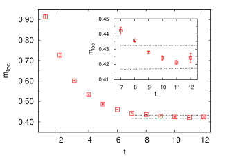
Figure 2: Local mass, $m_{loc}$ obtained from a measurement of the pion correlation function with staggered quarks on $24^{4}$ lattice with periodic boundary conditions at $\beta=5.6$ and bare quark mass $ma=0.025$. A close look shows that there is no plateau in $m_{loc}$ as $t$ changes.

In [8] we had reported a measurement of the pion mass using two flavours of staggered quarks in a $24^{4}$ lattice at $\beta=5.6$ and with bare quark mass $ma=0.025$. The best estimate was $m_{\pi}a=0.425\pm 0.008$. This was close to, but not in good agreement with, an earlier estimate [9] of $m_{\pi}a=0.415\pm 0.002$ which was made on smaller or comparable lattices.

However, a closer look at the plot of local masses, shown in Figure 2, shows that the estimate is not very satisfactory, since the local mass never seems to reach a plateau on lattices of this size. This is odd, since $m_{\pi}L\simeq 10$, and it would seem that this lattice size should be more than adequate for the extraction of this mass. This result can mean that at least one of the excited states cannot be easily decoupled from the ground state, either because it lies close in mass or because the operator used to excite a pion couples more strongly to one or more of these excited state.

In either case it would be possible to create several different kinds of sources with the same quantum number in order to perform a variational computation which isolates the ground state. This is the preferred method today [10]. However, it is also possible to adapt the MCF in [1] to this problem. In principle this yields a black-box similar to machine-learning applications today. It would be interesting also to combine the two methods in future.

The statistical analyses of the Goldstone pion correlators and local masses are discussed in detail in [8]. Errors on the local masses are calculated through a statistical bootstrap, nesting bootstrap loops where necessary. When the local mass is not constant, then the approximation of keeping only one state in eq. (2) fails, and one must keep at least one more mass in the hierarchy of eq. (1). Fitting the correlator keeping at least two states involves fitting 4 constants.

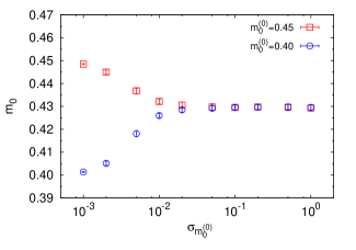
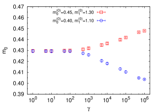
Figure 3: (Upper panel) The best fit value of $m_{0}$ changes systematically with the nuisance parameter $\sigma^{(0)}_{m_{0}}$ in MCF. For small values of this parameter the best fit to the mass is determined largely by the prior. However, for larger values, the best fit does not depend on $m_{0}^{(0)}$. (Lower panel) The dependence on the nuisance parameter $\gamma$ in MEM is the inverse. Both these figures are for the analysis of pion masses at $\beta=5.6$ and bare quark mass $ma=0.025$.

In the MCF we write the prior values $m_{0}^{0}$, $m_{1}^{0}$, $A_{0}^{0}$, $A_{1}^{0}$, and the corresponding meta-parameters $\sigma^{0}_{m_{0}}$, $\sigma^{0}_{m_{0}}$, $\sigma^{0}_{A_{0}}$, $\sigma^{0}_{A_{1}}$ for the parameters in eq. (1). In the MEM, priors carry the same notations as in MCF and there is a single meta-parameter $\gamma$. We show in Figure 3 that as the meta-parameter is tuned away from overconfidence a stable fit is obtained that is not very sensitive to the initial bias in the physical parameters. We quantify this further in the following way. For the MCF we choose priors in the large 8-dimensional hypercube with $m_{0}$ and $m_{1}$ allowed to vary between 0.1 and 1, $A_{0}$ varying in the range from $10^{-3}$ to 0.1, $A_{1}$ taking values between $10^{-7}$ and $10^{-5}$, and all the meta-parameters allowed to vary between 0.1 and 10. Within this hypercube we sampled points using the low-discrepancy Halton sequence [11]. We found that a little over 50% of the volume of priors gave results with 68% confidence limits of our best estimate for $m_{0}$, more than 95% of priors yielded a fit value within 95% confidence limits, and the full volume yielded results within 99% confidence limits. Similar results were obtained in the MEM. This indicates that prior bias is not a major issue.

Using this method, we have the estimate of the ground state pion mass is

$$am_{0}=0.429\pm 0.002$$ (19)

$$(\beta=5.6,\ am=0.025,\ N_{f}=2,\ {\rm pion})$$

with the 68% confidence limit on it, as shown in Figure 3. Exactly the same result is obtained on changing the Bayesian analysis from MEM to MCF. The distribution of the fitted parameter is strongly non-Gaussian, as can be seen from the fact that the 95% confidence limits are $0.429^{+0.052}_{-0.013}$. The above-calculated value of the ground state mass is consistent with the previously reported value [9], at the 95% confidence limit.

We are also able to obtain a similarly stable value for one excited state

$$am_{1}=1.21\pm 0.03$$ (20)

$$(\beta=5.6,\ am=0.025,\ N_{f}=2,\ {\rm pion})$$

at the 68% confidence level. Note that the difference $a\Delta m=am_{1}-am_{0}\simeq 0.78$ is large. This implies that the problem in disentangling the ground state probably comes from the fact that the composite operator used to excite a pion has a small overlap with the ground state.

According to the criteria discussed already after eq. (1), since $am_{1}>1$, we should stop at using only one excited state. The lattice lacks sensitivity to multiple excited states with masses above the lattice cutoff. In fact, if we use a third state, with mass $m_{2}$, and a corresponding coefficient $A_{2}$, in eq. (1), further complications arise. The fits tend to $m_{1}\simeq m_{2}$ with $A_{1}$ and $A_{2}$ varying wildly. We find that a stable fit can only be obtained if one imposes the restrictions $m_{2}\gg m_{1}$ and $A_{2}\ll A_{1}$. This is again an indication that there are only two masses smaller than or around the inverse lattice spacing. Scanning the meta-parameters, and priors with the restrictions above, yields the same stable value of $m_{0}$.

One way of quantifying the need to include an excited state is to examine how large a fraction of the correlator at $t=0$ is contained in the ground state term in eq. (1). Using the measured value, $C(0)$, of the correlator at $t=0$ and the fitted ground state parameters $am_{0}$ and $A_{0}$, we define the ground state overlap as the ratio

$$\Omega=\frac{A_{0}\cosh(am_{0}N_{t}/2)}{C(0)}$$ (21)

In the unlikely case in which $\Omega=1$, the full correlation function, even at distance $t=0$ would be described by a single state. We find that $\Omega=0.318\pm 0.009$ for this set. Although more than two-thirds of the correlation function come from excited states, the first excited state mass is already at the UV cutoff $1/a$, and one cannot resolve the tower of states above it.

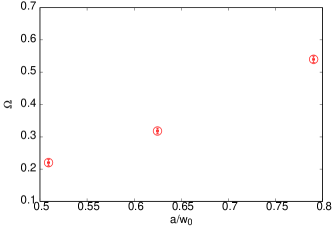
Figure 4: The ground state overlap obtained as explained here at $\beta=5.5$, 5.6 and 5.7 with bare quark mass $ma=0.025$. The lattice spacing in units of $w_{0}$ is taken from [8]. With decreasing lattice spacing the point source has rapidly decreasing overlap with the ground state.

We are able to do a similar analysis at $\beta=5.7$ and bare quark mass $ma=0.025$. Using two terms of the tower in eq. (1) we find

$$am_{0}=0.407^{+0.005}_{-0.006}$$ (22)

$$(\beta=5.7,\ am=0.025,\ N_{f}=2,\ {\rm pion})$$

where the errors are at the 68% confidence limit. This data set gives a more nearly Gaussian distribution of the fitted mass, with the errors doubling at the 95% confidence limit. A previous measurement [12] gave a similar value namely $am_{\pi}=0.388\pm 0.001$.

We show the ground state overlap as a function of the lattice spacing in Figure 4. One sees that a roughly 30% change in the lattice spacing causes the overlap to decrease by about a factor of two. It is interesting that the same Bayesian analysis can remove the contamination of masses by higher-lying states even though the overlap decreases so strongly. Extraction of the pion decay constant using the ground state amplitude $A_{0}$ shows that lattice spacing effects are small at fixed pion mass, when both are extracted in physical units. As a result, we found that the technique is a good black box even when the local mass plateau is not fully developed. In these cases we found that the excited state is non-physical, so the use of the modern machinery of variational computations [10] to simultaneously fit ground and multiple excited states is too ponderous.

4 Conclusions

In this paper we have examined the Bayesian approach to parameter extraction when all the parameters are not determined by the data. We have shown that meta-parameters, which we have called overconfidence, cause the solution to cross over from a prior dominated to a data dominated region in the best of the cases. When this happens, then a reasonable way to deal with the meta-parameters is to take them to lie in the region where the solution is data driven.

We applied this idea to extracting the lowest mass on a lattice which is too short for the local masses to show a plateau. This is usually due to (at least) one other state which has not decoupled since the lattice is not long enough. Rough estimates of the ground state and an excited state can often be made from inspection of the data. We showed that in the multi-parameter space of priors, convergence to a stable value is obtained once the meta-parameters are fixed using the notions developed in the previous section. This is, of course, the statement that the prior bias is not important once the overconfidence parameters have been dialled down. As a result, there is a black-box method for the fit.

We showed that fitting correlators with eq. (1) using MCF and MEM gave results consistent with other published estimates at the 95% confidence limits. We have checked that a simple-minded fit to local masses also gives results consistent with the above-mentioned estimates. However, the fit to correlators using eq. (1) is to be preferred since it makes weaker assumptions about the data. Our results mildly correct previous measurements of the pion mass at the same values of bare parameters.

An interesting physics result is given in Figure 4 where we show quantitatively how the overlap of a point source on the physical pion decreases with the lattice spacing. Interestingly, we showed that although the ground state overlap decreases, the excited states which couple to the operators are above the lattice cutoff. The variational methods which are used today [10] to project on to the ground state are too expensive, since the simultaneous extraction of excited state properties will not give physics results. In such cases the simple black-box method that we describe becomes useful.