Reconstruction of Past Human land-use from Pollen Data and Anthropogenic land-cover Changes Scenarios

Abstract

Accurate maps of past land cover and human land-use are necessary when studying the impact of anthropogenic land-cover changes on climate. Ideally the maps of past land cover would be separated into naturally occurring vegetation and human induced changes, allowing us to quantify the effect of human land-use on past climate. Here we investigate the possibility of combining regional, fossil pollen based, land-cover reconstructions with, population based, estimates of past human land-use. By merging these two datasets and interpolating the pollen based land-cover reconstructions we aim at obtaining maps that provide both past natural land-cover and the anthropogenic land-cover changes.

We develop a Bayesian hierarchical model to handle the complex data, using a latent Gaussian Markov random fields (GMRF) for the interpolation. Estimation of the model is based on a block updated Markov chain Monte Carlo (MCMC) algorithm. The sparse precision matrix of the GMRF together with an adaptive Metropolis adjusted Langevin step allows for fast inference. Uncertainties in the land-use predictions are computed from the MCMC posterior samples.

The model uses the pollen based observations to reconstruct three composition of land cover; Coniferous forest, Broadleaved forest and Unforested/Open land. The unforested land is then further decomposed into natural and human induced openness by inclusion of the estimates of past human land-use. The model is applied to five time periods - centred around 1900 CE, 1725 CE, 1425 CE, 1000 and, 4000 BCE over Europe. The results suggest pollen based observations can be used to recover past human land-use by adjusting the population based anthropogenic land-cover changes estimates.

1 Introduction

Human activities mainly influences the climate through the emission of greenhouse gases and anthropogenic land-cover changes (ALCC) (Kalnay and Cai, 2003). The effects of both natural and human induced land-cover changes on climate have been investigated in several simulation studies at both global (e.g. Claussen et al., 2001; Brovkin et al., 2002; Bala et al., 2007; Betts et al., 2007; Pitman et al., 2009; Pongratz et al., 2009; Christidis et al., 2013; Armstrong et al., 2016) and regional scales (e.g. Kalnay and Cai, 2003; Strandberg et al., 2014).

Historic ALCC consists mainly of deforestation to allow for agriculture and urbanization (Ruddiman, 2005). The temperate latitudes simulation studies indicate that replacing forests with agricultural land tends to decrease the radiative forcing (and thus temperature) (Bala et al., 2007; Betts et al., 2007), while observational studies show local temperature increases due to urbanization (Kalnay and Cai, 2003). The temperature decreases due to human deforestation are, to some extent, balanced by greenhouse gas emission due to the deforestation ($\text{CO}_{2}$) and farming practices (Methane) on the deforested land (Ruddiman, 2005; Kaplan, 2013). Earth system models that include dynamic vegetation, allowing for feedback between changes in climate, global $\text{CO}_{2}$-levels, and vegetation, give an even more complex picture. For these models the effects of ALCC depends on the global $\text{CO}_{2}$-levels, the climate region, and the natural land-cover replaced by human land-use (Armstrong et al., 2016).

Comparing historical temperature records with past natural land-cover and ALCC might improve our understanding of interactions among climate, land cover, and human land-use (Strandberg et al., 2014). However, descriptions of both past natural land-cover (e.g. Brovkin et al., 2002; Strandberg et al., 2011; Hickler et al., 2012) and past ALCC scenarios (e.g. Kaplan et al., 2009; Pongratz et al., 2009; Klein Goldewijk et al., 2011) varies considerably (Gaillard et al., 2010). It was previously shown that fossil pollen records can be used to reconstruct past vegetation and land cover at both local (Sugita, 2007a), regional (Sugita, 2007b; Paciorek and McLachlan, 2009; Sugita et al., 2010), and continental scales (Pirzamanbein et al., 2014).

This paper investigates the possibility of reconstructing both past natural land-cover and the ALCC by extending the Bayesian hierarchical model introduced by Pirzamanbein et al. (2018). The fossil pollen data can be used to obtain past land cover (Sugita, 2007b), but does not distinguish naturally open land from deforestation caused by ALCC. Ideally we would like to combine land-cover estimates based on fossil pollen records with archaeological data. However, initial studies of available archaeological data revealed a number of potential issues (see discussion in Section 5.1).

To investigate if the modelling is possible we instead used ALCC scenarios (Kaplan et al., 2009; Klein Goldewijk et al., 2011) as an estimate of past ALCC. The resulting model can be seen as an adjustment of the ALCC scenarios based on information in the pollen records (The available data is described in Section 2). The reconstruction is done across Europe for five time periods — centred around 1900, 1725, 1425 CE and 1000, 4000 BCE. These time periods represent important historical periods (recent past, little ice age, black death, late bronze age, and early Neolithic) and are commonly used in both climate modelling and palaeoecological studies. In Section 5.1 we outline one way of extending the model to include archaeological data, and we hope that our results will encourage the development of archaeological databases, that can be used in future modelling.

The model presented here (see Section 3) considers the pollen based land-cover data to be Dirichlet observations and the ALCC scenarios to beta observations of underlying latent fields. The spatial structure in the latent fields is modelled using covariates and Gaussian Markov Random Fields (Lindgren et al., 2011). The model is estimated using a Markov chain Monte Carlo (MCMC) algorithm based on the Metropolis Adjusted Langevin algorithm (MALA) (Girolami and Calderhead, 2011). Results are presented in Section 4 and Section 5 concludes the analysis with a discussion.

2 Data

The available data consist of fossil pollen based land-cover data, estimates of past human land-use (ALCC scenarios) and potential covariates (elevation and output from a dynamic vegetation model – DVM).

2.1 Pollen based land-cover compositions

Pollen based estimates of three land-cover compositions (LCCs), Coniferous forest (C), Broadleaved forest (B) and Unforested land (U), were obtained from the LANDCLIM project (Gaillard et al., 2010) using the REVEALS model (Sugita, 2007b). These three land-cover types are commonly used in studies of past climate and climate modelling (Strandberg et al., 2014). REVEALS is a mechanistic model which uses inter-taxonomic differences in pollen productivity, dispersal and the size of sedimentary basins to estimate regional land-cover from pollen records. The sedimentary pollen records used by REVEALS are obtained from lakes and bogs and presented as grid based REVEALS estimates for the $1^{\circ}\times 1^{\circ}$ grid cells containing sampled lakes and/or bogs (Hellman et al., 2008, showed that the spatial scale of REVEALS reconstructions is around $100\times 100$ km). The resulting land-cover data consists of pollen based LCCs for respectively 175, 181, 193, 204 and 196 grid cells during the five time periods centred around 1900, 1725 and 1425 CE, 1000 and 4000 BCE (Trondman et al., 2015). For use in climate modelling these sparse LCC observations can be interpolated to continuous spatial maps (Pirzamanbein et al., 2018). Here we will perform the interpolation while also trying to separate the LCC into natural vegetation and ALCC.

2.2 Anthropogenic land-cover change scenarios

Two anthropogenic land-cover change (ALCC) scenarios are used as estimates of human land-use: 1) The Kaplan and Krumhardt 2010 scenario (KK10; Kaplan et al., 2009), and 2) The History Database of the Global Environment (HYDE; Klein Goldewijk et al., 2011) . KK10 and HYDE are both based on historic human population density estimates, the land needed to feed that population, and soil productivity. To match the pollen records, the two estimates of human land-use were upscaled (by averaging) to the $1^{\circ}\times 1^{\circ}$ grid cells.

The KK10 and HYDE datasets differ substantially for the older time periods (see Fig. 1), due to differences in assumptions, modelling approaches, and historical records used. In general KK10 gives higher estimates of human land-use. Both datasets exhibit substantial local structure.

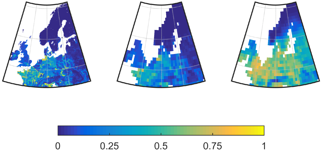
Figure 1: Anthropogenic land-cover changes (ALCC) scenarios for 1400 CE. From left to right: The high-resolution ($5^{\prime}$ or about $10$ km) HYDE ALCC scenario (Klein Goldewijk et al., 2011), HYDE upscaled to $1^{\circ}$ resolution matching the pollen data, and the KK10 (Kaplan et al., 2009) ALCC scenario at $1^{\circ}$ resolution.

2.3 Covariates

To capture large scale structures in the LCC, covariates consisting of elevation (from the Shuttle Radar Topography Mission, Becker et al., 2009) and model based vegetation estimates can be used (Pirzamanbein et al., 2017).

The model based estimates of potential natural vegetation were obtained by running a process-based dynamic vegetation model (DVM), LPJ-GUESS, (Smith et al., 2001) for the study area and specified time periods. LPJ-GUESS estimates the potential natural vegetation based on bio-climatic variables such as temperature, precipitation, and soil types (see Pirzamanbein et al., 2014, for details regarding the LPJ-GUESS runs).

3 Model

For the modelling we assume that each grid cell has a natural LCC, ${\boldsymbol{p}}_{L}=(p_{C},p_{B},p_{U})$, representing the proportion of each grid cell that would be coniferous, broadleaved, or unforested without any human activity. Additionally we let $p_{H}$ denote the share of each grid cell that is affected by ALCC. Since the ALCC data represents human land-use for food production we assume that all human land-use can be seen as a replacement of the corresponding proportion of natural land-cover with open land. The resulting link between natural and actual land cover, ${\boldsymbol{z}}=(z_{C},z_{B},z_{U})$, is

$$\begin{split}z_{C}&=p_{C}(1-p_{H}),\\ z_{B}&=p_{B}(1-p_{H}),\\ z_{U}&=p_{U}(1-p_{H})+p_{H},\end{split}$$

with the transformation being denoted ${\boldsymbol{z}}=h({\boldsymbol{p}}_{L},p_{H})$ (compare to the covariate adjustments in Pirzamanbein et al., 2014).

The pollen based land-cover compositions ${\boldsymbol{L}}=(L_{C},L_{B},L_{U})$ are now seen as Dirichlet distributed observations of the actual land cover, ${\boldsymbol{z}}$. Similarly the ALCC proportions $H$ are modelled as draws from beta distributions with expectation $p_{H,k}$, where $p_{H,k}$ are perturbations of $p_{H}$ introduced to handle the (large) differences between the two ALCC datasets (see Figure 1). The resulting model for the pollen and ALCC data given the underlying proportions is

$$\begin{split}{\boldsymbol{L}}({\boldsymbol{s}})|\alpha,{\boldsymbol{z}}({\boldsymbol{s}})&\sim\mathsf{Dir}\left(\alpha,{\boldsymbol{z}}({\boldsymbol{s}})\right),\\ H_{k}({\boldsymbol{s}})|\lambda,p_{H,k}({\boldsymbol{s}})&\sim\mathsf{Beta}\left(\lambda p_{H,k}({\boldsymbol{s}}),\lambda(1-p_{H,k}({\boldsymbol{s}}))\right).\end{split}$$ (1)

Here ${\boldsymbol{s}}$ is the location of each grid cell and $\alpha$ and $\lambda$ are concentration parameters controlling the uncertainty in the Dirichlet and beta distributions.

We model the grid cell proportions ${\boldsymbol{p}}_{L}({\boldsymbol{s}})=(p_{C}({\boldsymbol{s}}),\,p_{B}({\boldsymbol{s}}),\,p_{U}({\boldsymbol{s}}))$ and $p_{H}({\boldsymbol{s}})$ as a transformation of an multivariate latent field ${\boldsymbol{\eta}}({\boldsymbol{s}})$,

$${\boldsymbol{p}}_{L}({\boldsymbol{s}}) =f\bigl{(}{\boldsymbol{\eta}}_{L}({\boldsymbol{s}})\bigr{)}, p_{H}({\boldsymbol{s}}) =g\bigl{(}\eta_{H}({\boldsymbol{s}})\bigr{)}$$

with $f:\mathbb{R}^{2}\rightarrow(0,1)^{3}$ and $g:\mathbb{R}\rightarrow(0,1)$. For $f$ we use the inverse additive log-ratio transformation (applied for each grid cell, ${\boldsymbol{s}}$),

$$\begin{split}{\boldsymbol{\eta}}_{L}&=\left(\log\left(\dfrac{p_{C}}{p_{U}}\right),\log\left(\dfrac{p_{B}}{p_{U}}\right)\right)=\left(\eta_{L_{1}},\eta_{L_{2}}\right)\\ p_{\bullet}&=\begin{cases}\dfrac{\exp(\eta_{L_{i}})}{1+\sum_{i}\exp(\eta_{L_{i}})}&\text{for $p_{C}$ and $p_{B}$ with $i=1,2$,}\\ \vspace{-0.3cm}&\\ \dfrac{1}{1+\sum_{i}\exp(\eta_{L_{i}})}&\text{for $p_{U}$.}\end{cases}\end{split}$$ (2)

and for $g$ the inverse logit transformation

$$\eta_{H} =\log\left(\dfrac{p_{H}}{1-p_{H}}\right) p_{H} =\dfrac{\exp(\eta_{H})}{1+\exp(\eta_{H})}.$$ and (3)

The components of the latent field ${\boldsymbol{\eta}}({\boldsymbol{s}})$ are collected into a column vector and modelled using a mean part, ${\boldsymbol{B}}{\boldsymbol{\beta}}$, and a component capturing spatial dependencies ${\boldsymbol{X}}$:

$$\begin{split}{\boldsymbol{\eta}}&=\begin{bmatrix}{\boldsymbol{\eta}}_{L_{1}}\\ {\boldsymbol{\eta}}_{L_{2}}\\ {\boldsymbol{\eta}}_{H}\end{bmatrix}={\boldsymbol{B}}{\boldsymbol{\beta}}+{\boldsymbol{X}}.\end{split}$$

Here ${\boldsymbol{B}}$ is a matrix of covariates, ${\boldsymbol{\beta}}$ is a vector of regression coefficients, and ${\boldsymbol{X}}$ is a multivariate spatial field.

For ${\boldsymbol{\eta}}_{H}$ covariates in ${\boldsymbol{B}}$ consist of an intercept and elevation. For ${\boldsymbol{\eta}}_{L}$ two possible sets of covariates consisting of either intercept and elevation; or intercept, elevation, and model based vegetation estimates (from LPJ-GUESS) will be evaluated. For the LPJ-GUESS covariates the DVM based 3-compositions of natural potential vegetation were transformed to $\mathbb{R}^{2}$ using (2), resulting in two covariates, LPJ-GUESS_1,2. The spatial field, ${\boldsymbol{X}}$, is modelled using a Gaussian Markov random field (GMRF, Rue and Held, 2004) with a separable covariance structure,

$${\boldsymbol{X}}\sim\mathsf{N}\left({\boldsymbol{0}},{\boldsymbol{\Sigma}}\otimes{\boldsymbol{Q}}(\kappa)^{-1}\right)$$

where ${\boldsymbol{\Sigma}}$ is a $3\times 3$ covariance matrix, ${\boldsymbol{Q}}(\kappa)$ is the precision matrix of a GMRF that approximates fields with Matérn covariance function (Lindgren et al., 2011; Lindgren and Rue, 2015), and $\kappa$ governs the range of the spatial dependence.

To handle the differences between the KK10 and HYDE data, perturbed proportions of human land-use $p_{H,k}({\boldsymbol{s}})$ were introduced in the data model, (1). These perturbations are created by adding random effects to the ${\boldsymbol{\eta}}_{H}$-field; $p_{H,k}({\boldsymbol{s}})$ is computed from $\eta_{H,k}({\boldsymbol{s}})=\eta_{H}({\boldsymbol{s}})+\epsilon_{k}$ using (3) where $\epsilon_{k}\sim\mathsf{N}\left(0,\tau_{\epsilon}^{-1}\right)$. Note that $\epsilon_{k}$ are common terms added to the entire field, an attempt to use different random effects for each grid cell, i.e. $\epsilon_{k}({\boldsymbol{s}})$, resulted in an unidentifiable model.

The full hierarchical model is illustrated in Figure 2. The final part of the model is to specify suitable priors, following (Pirzamanbein et al., 2018) we use wide priors for $\alpha$ and $\lambda$; conjugate priors for ${\boldsymbol{\Sigma}}$; for $\kappa$ we pick a prior appropriate to the size of our spatial domain (Fuglstad et al., 2016). For ${\boldsymbol{\beta}}$ we choose a grouped horseshoe shrinkage prior with global and local hyper-parameters $\varphi$ and $\gamma_{i}$. This shrinks insignificant coefficients towards zero aiding the variable selection. Hyper-parameters for $\gamma_{i}$ and $\varphi$ are given as the standard half-Cauchy distribution ($\mathsf{C}^{+}$) (Makalic and Schmidt, 2016). Finally we pick a conjugate prior for $\tau_{\epsilon}$ since this, similar to ${\boldsymbol{\Sigma}}$, allows for simple MCMC updates. The resulting priors are

$$\alpha \sim\mathsf{\Gamma}\left(1.5,0.1\right),\qquad\lambda\sim\mathsf{\Gamma}\left(1.5,0.1\right), \tau_{\epsilon} \sim\mathsf{\Gamma}\left(1.5,0.1\right),$$

$$\kappa \sim\mathsf{\Gamma}\left(1,\frac{\log(100)}{\sqrt{8}}\right), {\boldsymbol{\Sigma}} \sim\mathsf{IW}\left(\mathbb{I},10\right),$$

$$\beta_{ki}|\gamma_{i},\varphi \sim\mathsf{N}\left(0,\varphi^{2}\gamma_{i}^{2}\right), i =1\cdots p$$

$$\gamma_{i} \sim\mathsf{C}^{+}\left(0,1\right), \varphi \sim\mathsf{C}^{+}\left(0,1\right).$$

Figure 2: Directed acyclic graph describing the conditional dependencies in the hierarchical model.

3.1 Estimation using MCMC

To estimate model parameters and reconstruct the latent field we use a block-updated MCMC algorithm. In the first block the latent fields – ${\boldsymbol{\eta}}$, ${\boldsymbol{\beta}}$, and $\epsilon_{k}$ – and the Dirichlet and beta concentration parameters – $\alpha$ and $\lambda$ – are updated using a MALA proposal (Girolami and Calderhead, 2011) and the conjugate posterior for $\tau_{\epsilon}$, $\gamma$ and $\varphi$. In the second block, we update the range parameter of the GMRF – $\kappa$ – using a random walk in log scale and the covariance matrix – ${\boldsymbol{\Sigma}}$ – using the conjugacy (conditioned on $\kappa$). Finally $\tau_{\epsilon}$ is updated using the conjugate posterior. In each iteration the MCMC alternates between these three blocks. To get the desired acceptance rate we use an adaptive scheme (Andrieu and Thoms, 2008) where the step size of the MALA proposal and the random walk are adjusted to maintain $57\%$ and $40\%$ acceptance rate, respectively (Roberts et al., 2001). This MCMC is an extension of the implementation, for a simpler model, described by Pirzamanbein et al. (2018).

We ran $100\,000$ MCMC iterations with a burn-in sample size of $10\,000$ to estimates the parameters of each model. The MCMC chain plots show convergence and good mixing of the parameters.

4 Results and discussion

The reconstruction of human land-use, potential natural vegetation and land-cover compositions are shown in Figure 3 for the 1425 CE time period. The results for the other time periods are available in Appendix B. In general, the reconstructions capture the variability in the observed datasets. The human land-use reconstructions mostly capture the spatial patterns of KK10 while the amount of land-use is closer to HYDE. Moreover, the model with only elevation as covariates estimates slightly higher amounts of human land-use compared to the model also including LPJ-GUESS as covariates.

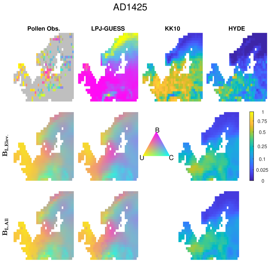
Figure 3: The observation datasets (row 1) and the reconstructions using two different sets of covariates (row 2 and 3) for 1425 CE. From left to right: land-cover composition, natural land-cover, and human land-use.

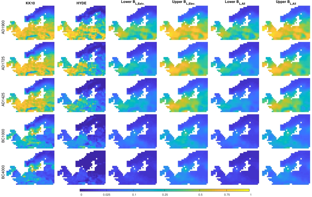
Figure 11: HYDE and KK10 observations and confidence bound for human land-use reconstructions, see page C.

The estimates of $\epsilon_{k}$ for HYDE and KK10 (Figure 4) also indicate that the human land-use reconstructions are, on average, closer to HYDE than KK10 for all the time periods. The difference between HYDE and KK10, as captured by $\epsilon_{k}$, increases for older time periods (see Figure 11 in Appendix. C). The estimates of $\epsilon_{k}$ are higher when the model includes both elevation and LPJ-GUESS as covariates compared to the model only including elevation. This is in accordance with the higher estimates of human land-use in the model containing only elevation.

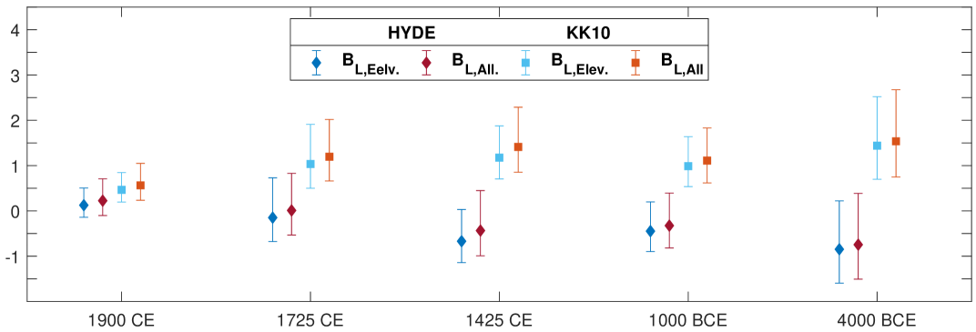
Figure 4: Estimated $\epsilon_{k}$ for HYDE and KK10 and corresponding $95\%$ confidence intervals for all time periods. The blue color represents model includes only elevation and red color represents model include both elevation and LPJ-GUESS.

The uncertainties in the human land-use reconstructions denote higher variation in the model with LPJ-GUESS as covariates than the model with only elevation (Figure 11 in Appendix. C). The uncertainty in the compositional reconstructions, i.e. natural potential land-cover and land-cover composition, are computed using transformed elliptical confidence regions (Pirzamanbein et al., 2018). The results together with confidence intervals for human land-use are illustrated in Figure 5 for three locations during the 1425 CE time period. The confidence regions are based on the model using only elevation, in order to allow a comparison between the NLC estimates and LPJ-GUESS. The selected point in the Baltic (column 1 in Figure 5) represents a location with contrasting values in the different data sources, i.e. about $70\%$ of coniferous forest in LCC, $70\%$ of broadleaved forest in LPJ-GUESS, and $40\%$ or $10\%$ of human land-use in KK10 and HYDE respectively. The differences among the data sources are balanced in the reconstruction of LCC, NLC and human land-use. In contrast, when the differences are smaller the confidence regions include the observations quiet well (columns 2 and 3 in Figure 5). The selected point in Scotland (column 3 in Figure 5) shows the improvement of the NLC reconstruction compared to the LPJ-GUESS estimate. The reconstruction suggests that the $80\%$ of unforested land consist of $10\%$ human land-use while LPJ-GUESS suggests $30\%$ unforested land and $70\%$ boardleaved forest.

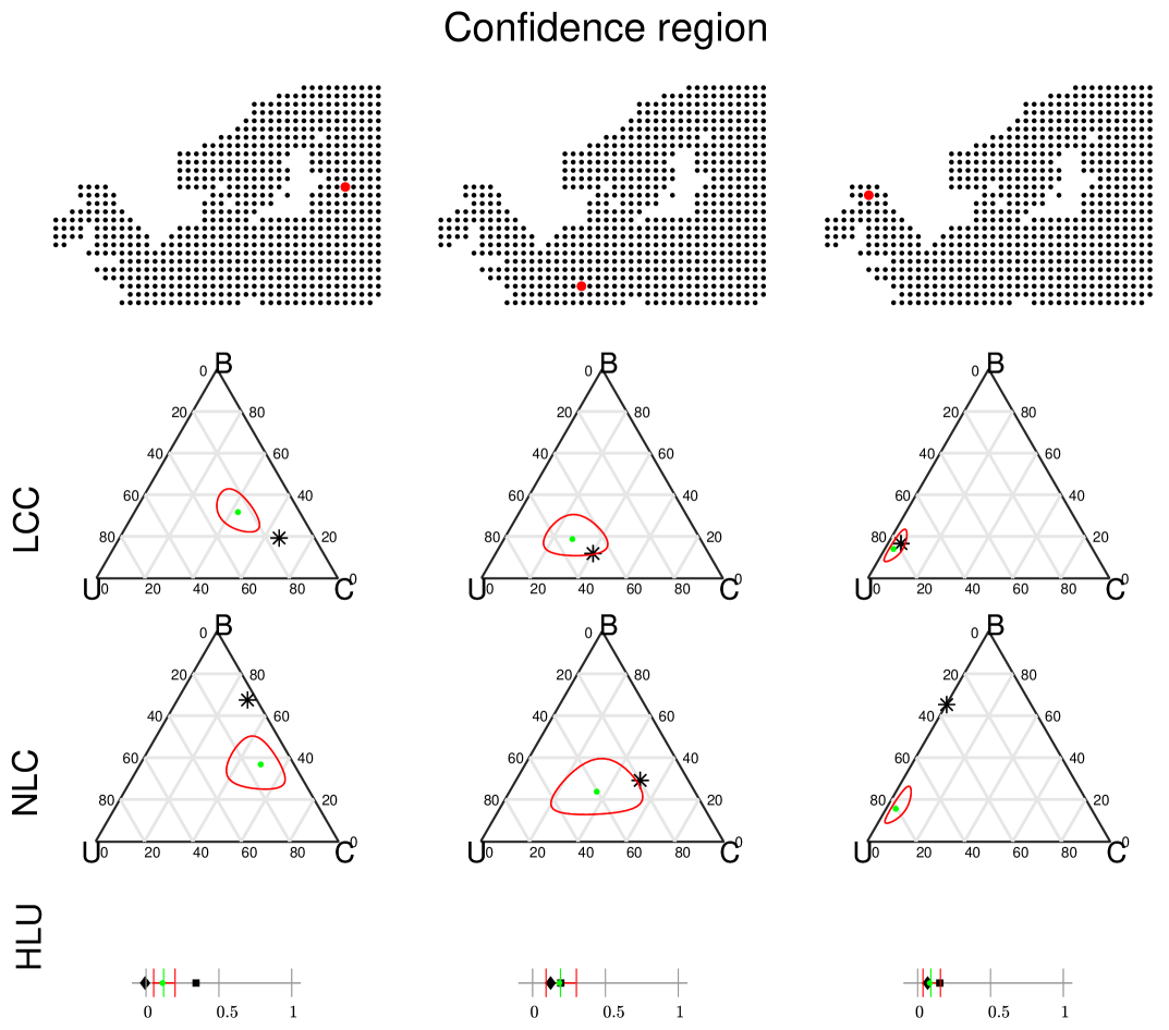
Figure 5: The reconstruction and prediction regions for three locations for land-cover composition (LCC), natural land-cover (NLC) and human land-use (HLU) for 1425 CE. For LCC and NLC (rows 2 and 3) the observations, pollen based REVEALS reconstructions and LPJ-GUESS output respectively, are marked with ($\ast$). For HLU (row 4) the two ALCC observations are given by HYDE (${\blacklozenge}$) and KK10 ($\blacksquare$). For all figures the green dots indicate estimated values and the red lines represent the corresponding confidence regions. All estimates and confidence regions are based on the model without LPJ-GUESS_1,2 as covariates.

A leave out validation is used to evaluate the performance of the model. The validation is performed by randomly removing $10\%$ of observed grid cells in the LCC and ALCC data and reconstruct these values based on the remaining observations. The resulting land-cover reconstructions are compared to LCC using average compositional distance (ACD; see Aitchison et al., 2000; Pirzamanbein et al., 2018), and the human land-use reconstructions are compared to both KK10 and HYDE using root mean squared error (RMSE). Comparing the ACD and RMSE (Table 1), there is no general preference in for any of the two models with different covariates. As has previously been noted the HLU estimates are, in general, closer to HYDE than to KK10.

ACD RMSE REV KK10 HYDE ${\boldsymbol{B}}_{\text{All}}$ ${\boldsymbol{B}}_{\text{Elev.}}$ ${\boldsymbol{B}}_{\text{All}}$ ${\boldsymbol{B}}_{\text{Elev.}}$ ${\boldsymbol{B}}_{\text{All}}$ ${\boldsymbol{B}}_{\text{Elev.}}$ 1900 CE 1.11 0.97 0.16 0.13 0.14 0.12 1725 CE 1.11 1.01 0.26 0.22 0.14 0.12 1425 CE 1.25 1.15 0.25 0.23 0.09 0.10 1000 BCE 1.17 1.14 0.14 0.13 0.05 0.06 4000 BCE 1.14 1.27 0.14 0.12 0.02 0.02

Table 1: Leave out validation results for models with two different sets of covariates, ${\boldsymbol{B}}_{\text{All}}$,${\boldsymbol{B}}_{\text{Elev.}}$ and all time periods. The reconstructions of land-cover compositions (LCC) are compared using average compositional distances (ACD). The human land-use (HLU) reconstructions are compared using root mean square error (RMSE). The bold number indicates the lowest value in the row for LCC and HLU.

5 Conclusion

In this paper, we developed a Bayesian hierarchical model to reconstruct the past human land-use for five time periods centred around 1900 CE, 1725 CE, 1425 CE, 1000 BCE and 4000 BCE. The reconstructions are based on combination of pollen based land-cover compositions (Trondman et al., 2015) and population based anthropogenic land-cover changes (ALCC) estimates.

Due to discrepancies between the past ALCC estimates, the model uses two different datasets of human land-use: • anthropogenic land cover changes scenario of Kaplan et al. (2009, KK10) and historic data base of global environment (HYDE; Klein Goldewijk et al., 2011) . The past human land-use reconstruction capture the spatial patterns of KK10 while being closer in value to the proportions of HYDE. This suggests that pollen based LCC can be used to adjust the existing population based human land use to match observed past vegetation patterns and recover past human land-use from pollen based LCC.

We note that the model would allow the inclusion of additional anthropogenic land-cover changes scenarios and it would be interesting to also include archaeological data. However, our initial attempts to use archaeological data have so far, as described below, been unsuccessful.

5.1 Including archaeological data in the model

We initially considered using archaeological data, instead of the ALCC scenarios, as a measure of human land-use. Given an archaeological dataset containing the locations of relevant archaeological finds during each of the five time periods we would replace the $\beta$-observations of the ALCC scenarios with a point process (Simpson et al., 2016) over the archaeological finds. The base idea being that more finds, in a given region, would correspond to a higher human activity and thus a higher proportion of ALCC.

One possible model would be an exponential link-function between the latent field, ${\boldsymbol{\eta}}_{H}$, and the intensity, ${\boldsymbol{\lambda}}$, of the point process for the archaeological finds, e.g.

$${\boldsymbol{\lambda}} =\exp\left({\boldsymbol{\eta}}_{H}\right)$$

$$\log\mathsf{P}({\boldsymbol{A}}|\lambda) =\left\lvert\Omega\right\rvert-\int_{\Omega}\lambda(s)\,\mathrm{d}s+\sum_{i=1}^{n}\log\lambda(s_{i})$$

where ${\boldsymbol{A}}=\{s_{i}\}$ are the locations of the archaeological finds. Since the point process provides the relative frequency of events, the latent field, ${\boldsymbol{\eta}}_{H}$, might only be determined up to an additive constant. To make the model identifiable the ALCC scenarios could still be needed, either as observations or as covariates. While it would be very interesting to investigate this model we have been unable to find a suitable archaeological dataset.

For us, a large detrimental factor to the use of archaeological data has been our inability to find archaeological databases covering the entire study area. One option considered was to restrict the modelling to Sweden using the Fornsök-database maintained by the Swedish National Heritage Board. This database contains information regarding roughly 1.7 million finds, but is incomplete with data contributions largely depending on the local municipalities (kommuner).

An initial search of the database resulted in $68\,000$ dated finds marked as relating to agricultural and/or settlement activities. And an additional $54\,000$ finds in these categories without any dating information. The spatial information regarding finds is good ($\pm 250$ m, i.e. much smaller than the spatial resolution of the pollen based LCCs). However, the dating information ranges from very good (based on $C_{14}$ or dendrochronology) to rather inexact. With most of the finds being dated based on typology, i.e. as belonging to one (or several) of 5 time periods. The wide ranges of possible dates and the uncertainty regarding selection bias due to differing priorities among the contributing municipalities makes the data unsuitable for our purposes (see Fig. 6).

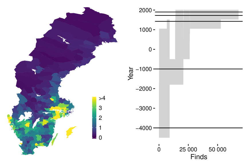
Figure 6: Overview of the Swedish archaeological data. The left pane shows the total number of finds per square kilometer for each of the 290 municipalities (kommuner) of Sweden. In the right pane the grey area indicates the dating range given for each archaeological find. The five time periods for which we have pollen data are indicated by the horizontal black lines.

Appendix A Computation for MALA proposal

For MALA proposal, the computation of the log density, first derivatives and expected Fisher information of the Beta distribution are required. The Fisher information is the negative expectation with respect to observations of the second and partial derivatives of the log density with respect to parameters and latent field.

A.1 Beta distribution computations

The Beta density is

$$\mathsf{P}({\boldsymbol{y}}|\lambda,{\boldsymbol{p}}) =\frac{\Gamma(\lambda)}{\Gamma(\lambda{\boldsymbol{p}})\Gamma(\lambda(1-{\boldsymbol{p}}))}{\boldsymbol{y}}^{\lambda{\boldsymbol{p}}-1}(1-{\boldsymbol{y}})^{\lambda(1-{\boldsymbol{p}})-1} \lambda >0,\ {\boldsymbol{p}}\in(0,1),$$

therefore the log density becomes

$$\begin{split}l=\log\mathsf{P}({\boldsymbol{y}}|\lambda,{\boldsymbol{p}})=&\log\Gamma(\lambda)-\log\Gamma(\lambda{\boldsymbol{p}})-\log\Gamma(\lambda(1-{\boldsymbol{p}}))\\ &+(\lambda{\boldsymbol{p}}-1)\log{\boldsymbol{y}}+(\lambda(1-{\boldsymbol{p}})-1)\log(1-{\boldsymbol{y}}).\end{split}$$

The first derivatives with respect to the parameters, $\lambda$ and ${\boldsymbol{p}}$ are

$$\begin{split}\dfrac{\partial l}{\partial\lambda}&=\psi(\lambda)-{\boldsymbol{p}}\psi(\lambda{\boldsymbol{p}})-(1-{\boldsymbol{p}})\psi(\lambda(1-{\boldsymbol{p}}))+{\boldsymbol{p}}\log{\boldsymbol{y}}+(1-{\boldsymbol{p}})\log(1-{\boldsymbol{y}}),\\ \dfrac{\partial l}{\partial{\boldsymbol{p}}}&=-\lambda\psi(\lambda{\boldsymbol{p}})+\lambda\psi(\lambda(1-{\boldsymbol{p}}))+\lambda\log{\boldsymbol{y}}-\lambda\log(1-{\boldsymbol{y}}).\end{split}$$

The second and partial derivatives are

$$\begin{split}\dfrac{\partial^{2}l}{\partial\lambda^{2}}=&\psi^{\prime}(\lambda)-{\boldsymbol{p}}^{2}\psi^{\prime}(\lambda{\boldsymbol{p}})-(1-{\boldsymbol{p}})^{2}\psi^{\prime}(\lambda(1-{\boldsymbol{p}})),\\ \dfrac{\partial^{2}l}{\partial{\boldsymbol{p}}^{2}}=&-\lambda^{2}\psi^{\prime}(\lambda{\boldsymbol{p}})-\lambda^{2}\psi^{\prime}(\lambda(1-{\boldsymbol{p}})),\\ \dfrac{\partial^{2}l}{\partial{\boldsymbol{p}}\partial\lambda}=&-\psi(\lambda{\boldsymbol{p}})-\lambda{\boldsymbol{p}}\psi^{\prime}(\lambda{\boldsymbol{p}})+\psi(\lambda(1-{\boldsymbol{p}}))+\lambda(1-{\boldsymbol{p}})\psi^{\prime}(\lambda(1-{\boldsymbol{p}}))\\ &+\log{\boldsymbol{y}}-\log(1-{\boldsymbol{y}}).\end{split}$$

The symmetric Fisher information is

$$\mathcal{I}=\begin{bmatrix}\mathcal{I}_{\lambda,\lambda}&\mathcal{I}_{\lambda,{\boldsymbol{p}}}\\ &\mathcal{I}_{{\boldsymbol{p}},{\boldsymbol{p}}}\end{bmatrix}=-\mathsf{E}_{\boldsymbol{y}}\begin{bmatrix}\dfrac{\partial^{2}l}{\partial\lambda^{2}}&\dfrac{\partial^{2}l}{\partial{\boldsymbol{p}}\partial\lambda}\\ &\\ &\dfrac{\partial^{2}l}{\partial{\boldsymbol{p}}^{2}}\end{bmatrix}$$

with elements

$$\begin{split}\mathcal{I}_{\lambda,\lambda}=&-\psi^{\prime}(\lambda)+{\boldsymbol{p}}^{2}\psi^{\prime}(\lambda{\boldsymbol{p}})+(1-{\boldsymbol{p}})^{2}\psi^{\prime}(\lambda(1-{\boldsymbol{p}}))\\ \mathcal{I}_{{\boldsymbol{p}},{\boldsymbol{p}}}=&\lambda^{2}\psi^{\prime}(\lambda{\boldsymbol{p}})+\lambda^{2}\psi^{\prime}(\lambda(1-{\boldsymbol{p}}))\\ \mathcal{I}_{\lambda,{\boldsymbol{p}}}=&-\psi(\lambda{\boldsymbol{p}})-\lambda{\boldsymbol{p}}\psi^{\prime}(\lambda{\boldsymbol{p}})+\psi(\lambda(1-{\boldsymbol{p}}))+\lambda(1-{\boldsymbol{p}})\psi^{\prime}(\lambda(1-{\boldsymbol{p}}))\\ &+\log{\boldsymbol{y}}-\log(1-{\boldsymbol{y}}).\end{split}$$

Since $\mathsf{E}(\log{\boldsymbol{y}})=\psi(\lambda{\boldsymbol{p}})-\psi(\lambda)$, $\mathcal{I}_{\lambda,{\boldsymbol{p}}}$ simplifies to

$$\begin{split}\mathcal{I}_{\lambda,{\boldsymbol{p}}}=\lambda{\boldsymbol{p}}\psi^{\prime}(\lambda{\boldsymbol{p}})-\lambda(1-{\boldsymbol{p}})\psi^{\prime}(\lambda(1-{\boldsymbol{p}})).\end{split}$$

Appendix B Maps of reconstructed land-cover and human land-use

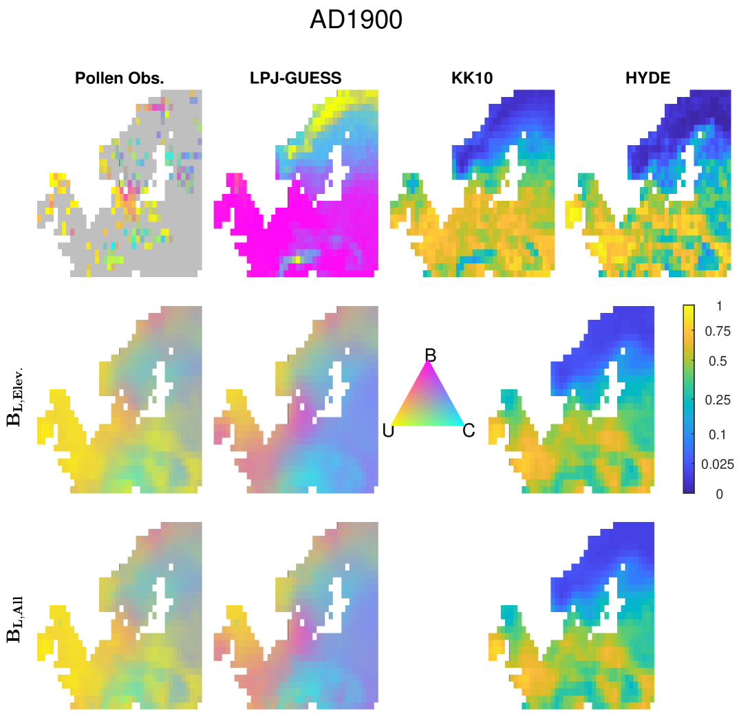
Figure 7: The observation datasets (row 1) and the reconstructions using two different sets of covariates (row 2 and 3) for 1900 CE. From left to right: land-cover composition, natural land-cover, and human land-use.

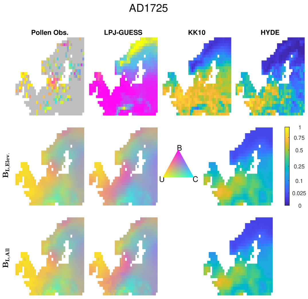
Figure 8: The observation datasets (row 1) and the reconstructions using two different sets of covariates (row 2 and 3) for 1725 CE. From left to right: land-cover composition, natural land-cover, and human land-use.

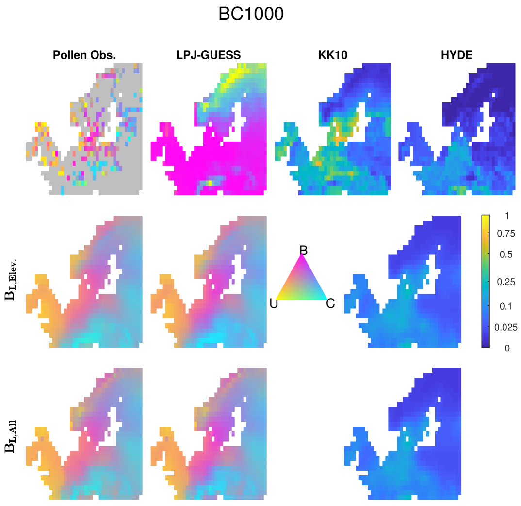
Figure 9: The observation datasets (row 1) and the reconstructions using two different sets of covariates (row 2 and 3) for 1000 BCE. From left to right: land-cover composition, natural land-cover, and human land-use.

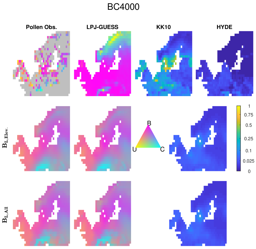
Figure 10: The observation datasets (row 1) and the reconstructions using two different sets of covariates (row 2 and 3) for 4000 BCE. From left to right: land-cover composition, natural land-cover, and human land-use.

Appendix C Uncertainties in land-use reconstruction

The desription of the figure in this appendix is as follows,
$95\%$ confidence interval for human land-use reconstructions for all time periods. From left to right: HYDE observations, KK10 observations, lower bound and upper bound for reconstruction of the model with only elevation as covariates, ${\boldsymbol{B}}_{\text{Elev.}}$, and lower bound and upper bound for reconstructions of the model with both elevation and LPJ-GUESS as covariates, ${\boldsymbol{B}}_{\text{All}}$.

References

- Aitchison et al. (2000) J. Aitchison, C. Barceló-Vidal, J. Martín-Fernández, and V. Pawlowsky-Glahn. Logratio analysis and compositional distance. Math. Geol., 32(3):271–275, 2000.
- Andrieu and Thoms (2008) C. Andrieu and J. Thoms. A tutorial on adaptive MCMC. Statist. and Comput., 18(4):343–373, 2008.
- Armstrong et al. (2016) E. Armstrong, P. Valdes, J. House, and J. Singarayer. The role of CO2 and dynamic vegetation on the impact of temperate land-use change in the HadCM3 coupled climate model. Earth Interactions, 20(10):1–20, 2016.
- Bala et al. (2007) G. Bala, K. Caldeira, M. Wickett, T. Phillips, D. Lobell, C. Delire, and A. Mirin. Combined climate and carbon-cycle effects of large-scale deforestation. Natl. Acad. Sci., 104(16):6550–6555, 2007.
- Becker et al. (2009) J. J. Becker, D. T. Sandwell, W. H. F. Smith, J. Braud, B. Binder, J. Depner, D. Fabre, J. Factor, S. Ingalls, S. H. Kim, R. Ladner, K. Marks, S. Nelson, A. Pharaoh, G. Sharman, R. Trimmer, J. VonRosenburg, G. Wallace, and P. Weatherall. Global bathymetry and elevation data at 30 arc seconds resolution: SRTM30_PLUS. Mar. Geod., 32(4):355–371, 2009.
- Betts et al. (2007) R. A. Betts, P. D. Falloon, K. K. Goldewijk, and N. Ramankutty. Biogeophysical effects of land use on climate: Model simulations of radiative forcing and large-scale temperature change. Agricultural and Forest Meteorology, 142(2–4):216–233, 2007.
- Brovkin et al. (2002) V. Brovkin, J. Bendtsen, M. Claussen, A. Ganopolski, C. Kubatzki, V. Petoukhov, and A. Andreev. Carbon cycle, vegetation, and climate dynamics in the Holocene: Experiments with the CLIMBER-2 model. Global. Biogeochem. Cy., 16(4):1139, 2002.
- Christidis et al. (2013) N. Christidis, P. A. Stott, G. C. Hegerl, and R. A. Betts. The role of land use change in the recent warming of daily extreme temperatures. Geophys. Res. Lett., 40(3):589–594, 2013.
- Claussen et al. (2001) M. Claussen, V. Brovkin, and A. Ganopolski. Biogeophysical versus biogeochemical feedbacks of large-scale land cover change. Geophys. Res. Lett., 28(6):1011–1014, 2001.
- Fuglstad et al. (2016) G.-A. Fuglstad, D. Simpson, F. Lindgren, and H. Rue. Interpretable priors for hyperparameters for Gaussian Random Fields. arXiv preprint arXiv:1503.00256, 2016.
- Gaillard et al. (2010) M.-J. Gaillard, S. Sugita, F. Mazier, A.-K. Trondman, A. Brostrom, T. Hickler, J. O. Kaplan, E. Kjellström, U. Kokfelt, P. Kuneš, , C. Lemmen, P. Miller, J. Olofsson, A. Poska, M. Rundgren, B. Smith, G. Strandberg, R. Fyfe, A. Nielsen, T. Alenius, L. Balakauskas, L. Barnekov, H. Birks, A. Bjune, L. Björkman, T. Giesecke, K. Hjelle, L. Kalnina, M. Kangur, W. van der Knaap, T. Koff, P. Lagerås, M. Latałowa, M. Leydet, J. Lechterbeck, M. Lindbladh, B. Odgaard, S. Peglar, U. Segerström, H. von Stedingk, and H. Seppä. Holocene land-cover reconstructions for studies on land cover-climate feedbacks. Clim. Past., 6:483–499, 2010.
- Girolami and Calderhead (2011) M. Girolami and B. Calderhead. Riemann manifold langevin and hamiltonian monte carlo methods. J. Roy. Statist. Soc. Ser. B, 73(2):123–214, 2011.
- Hellman et al. (2008) S. E. Hellman, M.-j. Gaillard, A. Broström, and S. Sugita. Effects of the sampling design and selection of parameter values on pollen-based quantitative reconstructions of regional vegetation: a case study in southern Sweden using the REVEALS model. Veg. Hist. Archaeobot., 17(5):445–459, 2008.
- Hickler et al. (2012) T. Hickler, K. Vohland, J. Feehan, P. A. Miller, B. Smith, L. Costa, T. Giesecke, S. Fronzek, T. R. Carter, W. Cramer, I. Kühn, and M. T. Sykes. Projecting the future distribution of European potential natural vegetation zones with a generalized, tree species-based dynamic vegetation model. Global. Ecol. Biogeogr., 21(1):50–63, 2012.
- Kalnay and Cai (2003) E. Kalnay and M. Cai. Impact of urbanization and land-use change on climate. Nature, 423(6939):528–531, 2003.
- Kaplan (2013) J. O. Kaplan. From forest to farmland and meadow to metropolis: What role for humans in explaining the enigma of Holocene CO2 and methane concentrations? In EGU General Assembly Conference Abstracts, volume 15, page 886, 2013.
- Kaplan et al. (2009) J. O. Kaplan, K. M. Krumhardt, and N. Zimmermann. The prehistoric and preindustrial deforestation of Europe. Quaternary. Sci. Rev., 28(27):3016–3034, 2009.
- Klein Goldewijk et al. (2011) K. Klein Goldewijk, A. Beusen, G. Van Drecht, and M. De Vos. The HYDE 3.1 spatially explicit database of human-induced global land-use change over the past 12,000 years. Global. Ecol. Biogeogr., 20(1):73–86, 2011.
- Lindgren and Rue (2015) F. Lindgren and H. Rue. Bayesian spatial modelling with R-INLA. J. Stat. Softw., 63(19), 2015.
- Lindgren et al. (2011) F. Lindgren, H. Rue, and J. Lindström. An explicit link between Gaussian fields and Gaussian Markov random fields: the stochastic partial differential equation approach. J. Roy. Statist. Soc. Ser. B, 73(4):423–498, 2011.
- Makalic and Schmidt (2016) E. Makalic and D. F. Schmidt. A simple sampler for the horseshoe estimator. IEEE. Signal. Process. Lett, 23(1):179–182, 2016.
- Paciorek and McLachlan (2009) C. J. Paciorek and J. S. McLachlan. Mapping ancient forests: Bayesian inference for spatio-temporal trends in forest composition using the fossil pollen proxy record. J. Am. Statist. Assoc., 104(486):608–622, 2009.
- Pirzamanbein et al. (2014) B. Pirzamanbein, J. Lindström, A. Poska, S. Sugita, A.-K. Trondman, R. Fyfe, F. Mazier, A. B. Nielsen, J. O. Kaplan, A. E. Bjune, H. J. B. Birks, T. Giesecke, M. Kangur, M. Latałowa, L. Marquer, B. Smith, and M.-J. Gaillard. Creating spatially continuous maps of past land cover from point estimates: A new statistical approach applied to pollen data. Ecol. Complex., 20(0):127–141, 2014.
- Pirzamanbein et al. (2017) B. Pirzamanbein, A. Poska, and J. Lindström. Bayesian reconstruction of past land-cover from pollen data: model robustness and sensitivity to auxiliary variables, 2017.
- Pirzamanbein et al. (2018) B. Pirzamanbein, J. Lindström, A. Poska, and M.-J. Gaillard. Modelling spatial compositional data: Reconstructions of past land cover and uncertainties. Spat. Stat., 24:14–31, 2018.
- Pitman et al. (2009) A. Pitman, N. de Noblet-Ducoudré, F. Cruz, E. Davin, G. Bonan, V. Brovkin, M. Claussen, C. Delire, L. Ganzeveld, V. Gayler, B. J. J. M. van den Hurk, P. J. Lawrence, M. K. van der Molen, C. Müller, C. H. Reick, S. I. Seneviratne, B. J. Strengers, and A. Voldoire. Uncertainties in climate responses to past land cover change: First results from the LUCID intercomparison study. Geophys. Res. Lett., 36(14), 2009.
- Pongratz et al. (2009) J. Pongratz, C. Reick, T. Raddatz, and M. Claussen. Effects of anthropogenic land cover change on the carbon cycle of the last millennium. Global. Biogeochem. Cy., 23(4):GB4001, 2009.
- Roberts et al. (2001) G. O. Roberts, J. S. Rosenthal, et al. Optimal scaling for various Metropolis-Hastings algorithms. Statist. Sci., 16(4):351–367, 2001.
- Ruddiman (2005) W. F. Ruddiman. How did humans first alter global climate? Sci. Am., March 2005:34–41, 2005.
- Rue and Held (2004) H. Rue and L. Held. Gaussian Markov random fields: theory and applications. CRC Press, 2004.
- Simpson et al. (2016) D. Simpson, J. Illian, F. Lindgren, S. Sorbye, and H. Rue. Going off grid: Computationally efficient inference for log-Gaussian Cox processes. Biometrika, 103(1):49–70, 2016.
- Smith et al. (2001) B. Smith, I. C. Prentice, and M. T. Sykes. Representation of vegetation dynamics in the modelling of terrestrial ecosystems: Comparing two contrasting approaches within European climate space. Global. Ecol. Biogeogr., 10(6):621–637, 2001.
- Strandberg et al. (2011) G. Strandberg, J. Brandefelt, E. Kjellström, and B. Smith. High-resolution regional simulation of last glacial maximum climate in Europe. Tellus. A, 63(1):107–125, 2011.
- Strandberg et al. (2014) G. Strandberg, E. Kjellström, A. Poska, S. Wagner, M.-J. Gaillard, A.-K. Trondman, A. Mauri, B. A. S. Davis, J. O. Kaplan, H. J. B. Birks, A. E. Bjune, R. Fyfe, T. Giesecke, L. Kalnina, M. Kangur, W. O. van der Knaap, U. Kokfelt, P. Kuneš, M. Latał owa, L. Marquer, F. Mazier, A. B. Nielsen, B. Smith, H. Seppä, and S. Sugita. Regional climate model simulations for Europe at 6 and 0.2 k bp: sensitivity to changes in anthropogenic deforestation. Clim. Past., 10(2):661–680, 2014.
- Sugita (2007a) S. Sugita. Theory of quantitative reconstruction of vegetation II: all you need is love. The Holocene, 17(2):243–257, 2007a.
- Sugita (2007b) S. Sugita. Theory of quantitative reconstruction of vegetation I: pollen from large sites REVEALS regional vegetation composition. The Holocene, 17(2):229–241, 2007b.
- Sugita et al. (2010) S. Sugita, T. Parshall, R. Calcote, and K. Walker. Testing the landscape reconstruction algorithm for spatially explicit reconstruction of vegetation in northern Michigan and Wisconsin. Quaternary. Res., 74(2):289–300, 2010.
- Trondman et al. (2015) A.-K. Trondman, M.-J. Gaillard, F. Mazier, S. Sugita, R. Fyfe, A. B. Nielsen, C. Twiddle, P. Barratt, H. J. B. Birks, A. E. Bjune, L. Björkman, A. Broström, C. Caseldine, R. David, J. Dodson, W. Dörfler, E. Fischer, B. van Geel, T. Giesecke, T. Hultberg, L. Kalnina, M. Kangur, P. van der Knaap, T. Koff, P. Kuneš, P. Lagerås, M. Latałowa, J. Lechterbeck, C. Leroyer, M. Leydet, M. Lindbladh, L. Marquer, F. J. G. Mitchell, B. V. Odgaard, S. M. Peglar, T. Persson, A. Poska, M. Rösch, H. Seppä, S. Veski, and L. Wick. Pollen-based quantitative reconstructions of holocene regional vegetation cover (plant-functional types and land-cover types) in europe suitable for climate modelling. Glob. Change Biol., 21(2):676–697, 2015.