Abstract

Low Earth orbit (LEO) satellites are being considered for expanding legacy terrestrial cellular networks. The end users may not be able to optimize satellite orbits and constellations, however, they can optimize locations of ground stations which aggregate terrestrial traffic and inter-connect with over-passing satellites. Such optimization requires a model of satellite visibility to decide when the satellite becomes visible to the ground station in a given geographical location. Our model assumes ideal Kepler orbits parameterized by six orbital elements to describe the satellite movements. The steps of Kepler orbit modeling are presented in detail to enable other studies requiring geometric representation of satellite trajectories in the 3D space or their 2D footprint on the Earth surface. The long-term mean time satellite visibility (MTSV) metric is defined to measure satellite visibility at a given ground station. Numerical results reveal that efficiency of optimizing the ground station locations is dependent on the satellite orbit and other satellite visibility constraints. The ground station location optimization is especially important when MTSV is improved by orthogonal time sharing schemes using multiple satellites on the same or different orbits. Similar conclusions can be drawn assuming other performance metrics such as the capacity of links between the ground station and the satellites.

Regional Coverage Analysis of LEO Satellites with Kepler Orbits Iestyn Morgan-Jones¹ and Pavel Loskot¹ Highlights

• A detailed model of Kepler orbit is presented, so it can be implemented in commonly available simulation software.

• Kepler orbit model yields celestial trajectories of satellites in the sky as well as the ground footprint trajectories.

• Simulating satellite trajectories is important to design and analyze satellite communication networks, to understand spatial geometry of satellite constellations, to model more realistic satellite communication channels and the associated terrestrial coverage, and to investigate communication protocols in satellite networks with given topology.

ECEF	Earth-centered Earth-fixed coordinates
ECI	Earth-centered inertial coordinates
GHA	Greenwich hour angle
GMST	Greenwich mean sidereal time
LEO	low Earth orbit
MRE	minimum required elevation
MTSV	mean time satellite visibility
RAAN	right ascension of ascending node

Constants

$398600.4$	$\left[\mathrm{km^{3}/s^{2}}\right]$	standard gravitational parameter wkp:standardgravpar
$6.3781\text{\times}{10}^{6}$	$\left[\mathrm{m}\right]$	Earth radius wkp:earthrad
$7.292\,115\,0\text{\times}{10}^{-5}$	$\left[\mathrm{rad/s}\right]$	Earth rotation angular speed wkp:earthrot
$1.727\,564\,3$	$\left[\mathrm{rad}\right]$	angular offset for Greenwich mean sidereal time wkp:sidertime

 

1 Introduction

Satellite technology is getting progressively cheaper due to advances in making the satellites smaller and lighter. This trend is supported by new aerospace enterprises who are starting to offer the cost affordable satellite launches into the orbit. Telecommunication services enabled by LEO satellite networks are particularly attractive due to their relative proximity to the Earth surface which reduces signal attenuations. The key design considerations for satellite networks are choosing appropriate satellite constellation, maintaining stable orbits, dynamically allocating frequency channels, and managing the connectivity and interference to terrestrial stations as well as in between satellites. However, satellite communication services are still rather expensive due to high initial (CapEx) and operational expenditures (OpEx), and the time constrained bandwidth sharing by a large pool of terrestrial users. In order to reduce the deployment times and costs while also minimizing the need for propulsive corrections at the orbit, small scale satellites are often launched together in batches and separated at the orbit to form the desired constellation Crisp et al. (2015).

The vision of a dense satellite network to provide the ubiquitous Internet access all over the Earth including basic capacity calculations for such network is presented in Khan (2016). The Quality-of-Service (QoS) issues in satellite mesh networks with delay-sensitive as well as delay-tolerant traffic are studied in Lee and Park (2019) assuming the link layer and network layer protocols. The link state routing for satellite networks having regular topology and embracing the whole Earth while experiencing uneven traffic distribution over different geographical areas is investigated in Wang et al. (2019). However, none of these works assume specific satellite trajectories. Precise observations of satellite trajectories require detailed understanding of orbital mechanics Clifford et al. (1994–2002). The main but not all steps for calculating Kepler orbits are presented in Zantou et al. (2005). Comprehensive review of satellite orbital mechanics is provided, for example, in Chobotov (2002) and in Vallado and McClain (1997). At lower altitudes up to about 800 km above the Earth surface, satellite orbits are more complex as their trajectories are subject to orbital decays due to residual atmospheric drag Bowman and Storz (2003). The upper atmosphere and gravity field are causing small changes in satellite movements referred to as perturbations. The Lagrangian perturbation forces are studied in Gergely (2015) to generalize Kepler laws of idealistic satellite motions to more realistic scenarios. The description of satellite trajectories, their ground tracks, orbits relative to the Earth, and modeling Earth views from the satellites can be found in Capderou (2005).

The problem of satellite constellation design to achieve the full Earth coverage has been addressed in Ballard (1980). The geometries of satellite constellations as a function of the inter-satellite distances and the maximum latitude to provide the continuous Earth coverage are investigated in Danesfahani and Pirhadi (2006). The capacity of satellite communication network created by some satellite constellations in different orbits is evaluated in Werner et al. (1995). The satellite constellation to maximize visibility from a given group of ground terminals is optimized in Chen et al. (2017). The methodology for calculating the mean visibility of satellite network from a ground station possibly equipped with the tracking antenna is developed in Rec. ITU-R S.1257 (1997). The long-term optimum locations of terrestrial stations having optical communication links to multiple satellites are investigated in Lyras et al. (2018). The optical satellite channels are affected by the presence of atmospheric clouds, so switching among terrestrial stations creates the transmission diversity. Accurate approximation of the closest approach for LEO satellites with the largest elevation to the ground terminal is derived in Ali et al. (1999). However, neither other orbital in-view periods which may also provide connectivity nor the minimum required elevation of the satellite above the horizon are considered. Typical value of the minimum elevation for a satellite to become visible is about $10^{\circ}$ Ali et al. (1998); Danesfahani and Pirhadi (2006). The coverage of a single LEO satellite at the fixed sky location is obtained in Pratt et al. (1999), and later elaborated in Cakaj et al. (2014). Assuming the circular LEO satellite orbits with uniformly distributed ground stations, the distribution of satellite in-view times are obtained in Seyedi and Safavi (2012). However, the analyses in Pratt et al. (1999); Cakaj et al. (2014); Seyedi and Safavi (2012) are limited in accounting for generally spatially non-synchronous trajectories of LEO satellites where every additional satellite overpass over the ground station is further shifted to the East or to the West.

Since satellites move over complex orbits, maintaining stable inter-satellite connectivity in large satellite constellations is rather challenging Hossain et al. (2017). The link performance in satellite channels is dominated by shadowing. Using empirical measurements, it was shown in Lutz et al. (1991) that satellite links fluctuate between good and bad transmission channels. The scattered multi-path components in satellite channels can be assumed to be Rayleigh distributed whereas Nakagami distribution is a good fit to empirical measurements for the line-of-sight component Abdi et al. (2003). The Doppler frequency shift of satellite channels is proportional to the satellite elevation above the ground station Ali et al. (1998).

Even though satellite constellations and orbits can be designed to maximize their visibility over a given geographical region, such option is rarely available to majority of terrestrial users. The users can, however, optimize the location of ground observation stations. Hence, in this paper, satellite visibility over a whole geographical region is evaluated numerically, so the locations of terrestrial stations can be optimized. The satellites are assumed to follow Kepler orbits. The satellite visibility is defined as the long-term mean in-view time from one or more terrestrial stations. The case of a single satellite station is the basic building block for evaluating the regional coverage of multi-satellite constellations.

It is found that the efficiency of optimizing the locations of terrestrial stations is dependent on the specific satellite orbit and on the minimum required elevation (MRE) of the satellite above the horizon. Selecting the ground station locations becomes even more important when orthogonal time sharing schemes are used with multi-satellite networks forming non-overlapping visibility windows in time. The detailed description of Kepler orbits is necessary to study satellite trajectories beyond simple circular orbits. Among research problems involving satellite spatial geometries are satellite communications. The orbits of satellite constellations affect the characteristics of satellite communication channels, the terrestrial coverage as well as topology and protocols of inter-satellite communication networks. Even though commercial software for calculating precise satellite trajectories exist, majority of researchers may prefer to implement Kepler orbits in their simulations in order to avoid possibly large financial costs for acquiring commercial software. It is of course possible to extend the model of Kepler orbits with additional features to improve the modeling accuracy of satellite trajectories. For example, the oblateness of the Earth induces drifts in the Kepler orbits, and for lower orbits, the atmospheric drag cannot be neglected.

The rest of this paper is organized as follows. Section 2 presents a detailed step-by-step model of Kepler orbits representing the satellite trajectory in 3D space including the corresponding 2D trajectory on the Earth surface. The satellite visibility is defined and analyzed in Section 3. Discussion in Section 4 concludes the paper. In our mathematical notation, $\left\|\mathbf{v}\right\|$ denotes the Euclidean norm of vector $\mathbf{v}$, $\hat{\mathbf{v}}=\mathbf{v}/\left\|\mathbf{v}\right\|$ is the unit length vector, $\mathbf{v}_{1}\times\mathbf{v}_{2}$ and $\mathbf{v}_{1}\cdot\mathbf{v}_{2}$ are the cross product and dot product of two vectors, respectively, and the components of 3D vectors are denoted as $\mathbf{v}=(v_{x},v_{y},v_{z})$.

2 Kepler orbits of LEO satellites

In many communications scenarios, it is sufficient to model satellite movements by assuming Kepler’s two-body mechanics. The resulting Kepler orbit describes the time dependent satellite trajectory in 3D space. Kepler orbit can be fully defined by the two vectors: initial position $\mathbf{r}(0)$ and initial speed $\mathbf{v}(0)$ at time $t=0$. These vectors represent a simple model of launching the satellite into a given orbit. The position and speed vectors $\mathbf{r}(t)$ and $\mathbf{v}(t)$, respectively, are normally expressed in the Earth-centered inertial (ECI) coordinates having the origin at the center of mass of the Earth while the axes do not rotate with the Earth wkp:ecicor . The vectors $\mathbf{r}(0)$ and $\mathbf{v}(0)$ can be used to calculate the six basic elements of Kepler orbit Chobotov (2002). The values of these elements fully define the orbit, so they can be specified instead of the initial vectors. Specifically, semi-major axis and eccentricity, respectively, describe the orbit size and shape. Inclination, right ascension (or longitude) of the ascending node (RAAN) and argument of perigee describe the orbit orientation in 3D space. Finally, true anomaly determines the satellite position in its orbit. Thus, the space of all Kepler orbits can be searched using either polar coordinates of vectors $\mathbf{r}$ and $\mathbf{v}$, or using the six orbital elements.

Eccentricity $e=\left\|\mathbf{e}\right\|$ is the magnitude of eccentricity vector wkp:excvec ; wkp:orbexc ; wkp:excanom ,

$$\mathbf{e}=\mathbf{v}\times\mathbf{h}/\mu-\hat{\mathbf{r}}$$

where the angular momentum vector $\mathbf{h}=\mathbf{r}\times\mathbf{v}$ wkp:angmom , and $\mu=G\cdot M_{E}=398600.4$ $\left[\mathrm{km^{3}/s^{2}}\right]$ is the standard gravitational parameter wkp:standardgravpar . The inclination angle $\iota$ of the orbit is computed as, $\iota=\cos^{-1}(\hat{\mathbf{h}}\cdot\mathbf{k}_{z})$ wkp:orbinc where the unit vector $\mathbf{k}_{z}=(0,0,1)$. Using the vis-viva equation wkp:visviva , the semi-major axis $a$ is calculated as wkp:semaxes ,

$$a=\left(2/\left\|\mathbf{r}\right\|-\left\|\mathbf{v}\right\|^{2}/\mu\right)^{-1}.$$

The RAAN angle $\Omega$ is calculated by first defining the vector $\mathbf{n}$ pointing towards the ascending node wkp:lonanode , i.e., let $\mathbf{n}=\mathbf{k}_{z}\times\mathbf{h}$, and,

$$\Omega=\left\{\begin{array}[]{cc}\cos^{-1}(n_{x}/\left\|\mathbf{n}\right\|)&n_{y}\geq 0\\ 2\pi-\cos^{-1}(n_{x}/\left\|\mathbf{n}\right\|)&\mbox{otherwise}.\end{array}\right.$$

The argument of periapsis $\omega$ is the angle from the ascending node to its periapsis measured in the direction of its motion wkp:argper , i.e., it is the angle between vectors $\mathbf{n}$ and $\mathbf{e}$ which can be calculated as,

$$\omega=\cos^{-1}(\hat{\mathbf{n}}\cdot\hat{\mathbf{e}}).$$

In order to determine the correct quadrant for $\omega$, we can also calculate,

$$\omega=\sin^{-1}\left(\frac{|\hat{\mathbf{n}}\times\hat{\mathbf{e}}|}{|\hat{\mathbf{n}}||\hat{\mathbf{e}}|}\right).$$

Finally, true anomaly $\nu$ is the angle between direction of periapsis and the current satellite position wkp:trueanom , i.e., it is the angle between the vectors $\mathbf{e}$ and $\mathbf{r}$. This angle can be calculated as,

$$\nu=\left\{\begin{array}[]{cc}\cos^{-1}\left(\frac{\mathbf{e}}{e}\cdot\hat{\mathbf{r}}\right)&\mathbf{r}\cdot\mathbf{v}\geq 0\\ 2\pi-\cos^{-1}\left(\frac{\mathbf{e}}{e}\cdot\hat{\mathbf{r}}\right)&\mbox{otherwise}.\end{array}\right.$$

In addition to the six basic orbital elements $\{e,\iota,a,\Omega,\omega,\nu\}$, it is useful to define the following parameters describing the satellite trajectory. In particular, mean anomaly is the angle the satellite would move along a hypothetical circular orbit having the same speed and the same orbital period wkp:meananom . It is calculated from the eccentric anomaly $E$ which is related to the true anomaly as,

$$\tan\frac{\nu}{2}=\sqrt{\frac{1+e}{1-e}}\,\tan\frac{E}{2},\mbox{ and }\sin E=\frac{\sqrt{1-e^{2}}\sin\nu}{1+e\,\cos\nu}.$$

The mean anomaly is then calculated as,

$$M=E-e\,\sin E.$$

Numerically, it is beneficial to calculate the mean anomaly $M_{0}$ at the initial epoch (i.e., the reference time) $t_{0}$, and then update the mean anomaly at time $t$ as wkp:meanmotion ,

$$M(t)=M_{0}+n(t-t_{0})$$

where $n=\sqrt{\mu/a^{3}}$ is the satellite angular frequency (i.e., the number of revolutions per unit of time). The new value of $E$ can be efficiently calculated from the updated mean anomaly using, for example, the Newton-Raphson iterations wkp:newrap .

The instantaneous radius $r=\left\|\mathbf{r}\right\|$ of the satellite orbit is calculated as, $r=a(1-e\cos E)$, where $r=R_{E}+h_{s}$, $R_{E}=6,378.1$ km is the Earth radius wkp:earthrad , and $h_{s}$ is the satellite altitude above the Earth surface. The semi-minor axis of Kepler orbit is computed as, $b=a\sqrt{1-e^{2}}$. The orbital period $T_{0}$ of the satellite is given by the Kepler’s third law wkp:keplaws , i.e.,

$$T_{0}=\sqrt{\frac{a^{3}4pi^{2}}{\mu}}.$$

Greenwich mean sidereal time (GMST) is used to measure longitude of the vernal equinox (i.e., the angle from prime meridian), accounting for the number of Earth rotations (measured in days) $J_{2000}$ since the 1st January 2000 wkp:sidertime . Assuming the angular speed of Earth rotations, $\omega_{E}=$7.292\,116\text{\times}{10}^{-5}$$ $\left[\mathrm{rad/s}\right]$ wkp:earthrot , the sidereal day duration of $86164$ seconds, and $G_{0}=1.727564$ being the Greenwich hour angle (GHA) corresponding to the 1st second of year 2000, we have,

$$\mathrm{GMST}_{0}=G_{0}+86164\,\omega_{E}(J_{2000}+1/2)\mod 2\pi.$$

The values of $\mathrm{GMST}$ are then simply updated as,

$$\mathrm{GMST}(t)=\mathrm{GMST}_{0}+(t-t_{0})2\pi/86164.$$

Finally, the instantaneous satellite position is expressed in the Earth-centered Earth-fixed (ECEF) coordinates wkp:ecefcor . The ECEF coordinates have the origin at the Earth center of mass, and they rotate with the Earth. The $x$-axis is passing through the vernal equinox (one of the two crossings of the ecliptic and the celestial equators), the $z$-axis is aligned with the Earth rotation axis, and the $y$-axis is perpendicular to the other two. Thus, after updating true anomaly $\nu$, and the current radius $r$, the current ECEF coordinates of the satellite are expressed in polar coordinates as,

$$X_{\mathrm{ecef}} = r\left(\cos(\omega+\nu)\cos(\Omega)-\sin(\omega+\nu)\sin(\Omega)\cos(\iota)\right)$$

$$Y_{\mathrm{ecef}} = r\left(\cos(\omega+\nu)\sin(\Omega)+\sin(\omega+\nu)\cos(\Omega)\cos(\iota)\right)$$

$$Z_{\mathrm{ecef}} = r\sin(\omega+\nu)\sin(\iota).$$

3 Satellite visibility

The ground track of the satellite is obtained by converting the ECEF coordinates to latitude $\phi_{s}$, longitude $\lambda_{s}$, and altitude $h_{s}$ using vectors,

$$\mathbf{g} = (\cos(\mathrm{GMST}),\sin(\mathrm{GMST}),0)$$

$$\mathbf{s}_{12} = (X_{\mathrm{ecef}},Y_{\mathrm{ecef}},0)$$

$$\mathbf{c} = \mathbf{g}\times\mathbf{s}_{12}=(c_{x},0,0).$$

We then obtain the ground track coordinates,

$$\phi_{s} = \tan^{-1}\left(\frac{Z_{\mathrm{ecef}}}{X_{\mathrm{ecef}}^{2}+Y_{\mathrm{ecef}}^{2}}\right)$$

$$\lambda_{s} = {\operatorname{sign}}\!\left(c_{z}\right)\,\mathrm{atan2}(\left\|\mathbf{c}\right\|,\mathbf{g}\cdot\mathbf{s}_{12})\mod 2\pi$$

where $\mathrm{atan2}$ is the 4-quadrant arc-tangent function, ${\operatorname{sign}}\!\left(\cdot\right)$ is the sign function, and the altitude $h_{s}=\left\|\mathbf{r}\right\|-R_{E}$. Our goal is to assess the satellite visibility from a ground station at specific location on the Earth surface at latitude $\phi_{p}$, longitude $\lambda_{p}$, and altitude $h_{p}=0$. The Earth rotation is accounted for by first computing the RAAN value,

$$\Omega_{p}=\mathrm{atan2}(\sin(\lambda_{p}+\mathrm{GMST}),\cos(\lambda_{p}+\mathrm{GMST})).$$

The ECI coordinates of the selected ground station location are given by the polar to Cartesian transformation,

$$X_{p} = (h_{p}+R_{E})\cos(\Omega_{p})\cos(\phi_{p})$$

$$Y_{p} = (h_{p}+R_{E})\sin(\Omega_{p})\cos(\phi_{p})$$

$$Z_{p} = (h_{p}+R_{E})\sin(\phi_{p}).$$

To decide on satellite visibility from a ground station, define vectors $\mathbf{s}=(X_{\mathrm{ecef}},Y_{\mathrm{ecef}},Z_{\mathrm{ecef}})$ of the current satellite orbital position, and $\mathbf{p}=(X_{p},Y_{p},Z_{p})$ of the observation point on the Earth surface. Assuming a 2D plane touching the Earth at the point $\mathbf{p}$, the satellite is visible as long as it is above the horizon represented by this plane. However, in realistic scenarios, local obstacles, satellite altitude and elevation as well as antenna radiation and reception patterns dictate the actual MRE of the satellite above the horizon in order it becomes visible at the ground station. Denoting such MRE value as $\epsilon_{\mathrm{mre}}$, the satellite visibility condition can be expressed mathematically using the cosine law, i.e.,

$$C_{1}:\ \frac{(\mathbf{s}-\mathbf{p})}{d_{sp}}\cdot\frac{\mathbf{p}}{R_{E}}\geq\cos\left(\frac{\pi}{2}-\epsilon_{\mathrm{mre}}\right)$$ (3)

where $d_{sp}=\left\|\mathbf{s}-\mathbf{p}\right\|$ denotes the distance between the satellite and the observation point, and we assume $\left\|\mathbf{p}\right\|=R_{E}$. Consequently, by increasing the value $\epsilon_{\mathrm{mre}}$, the satellite visibility time window during one overpass of the ground station is reduced by a factor,

$$f(\epsilon_{\mathrm{mre}})=1-\frac{2}{\pi}\,\epsilon_{\mathrm{mre}}.$$

3.1 Numerical analysis of LEO satellite visibility

Using the expressions defining Kepler orbit given in Section 2, it is straightforward to verify that the minimum satellite orbital speed to sustain its orbit is increasing with decreasing altitude. For instance, assuming circular orbit, the speeds greater than $\left\|\mathbf{v}\right\|\geq 7.1$ $\left[\mathrm{km/s}\right]$ are required for sustaining the orbital altitudes below $1530$ km. The orbits above 200 km up to about 2000 km above the Earth are classified as low Earth orbits. The sample footprint and altitude of a LEO satellite are shown in Figure 1 assuming the initial position and speed vectors $\mathbf{r}=(700+R_{E},0,0)$ [km] and $\mathbf{v}=7.5\times(0,\sqrt{2}/2,\sqrt{2}/2)$ [km/s]. For these initial vectors, the orbital period is $T_{0}=98.59$ min, i.e., about $14.56$ rotations in a day (i.e., in 86164 sec), so the satellite trajectory is not ground periodic (also referred to as Earth-repeat, or Earth synchronous Rec. ITU-R S.1257 (1997)). The Earth periodic orbit has to account for the Earth oblateness effect. For other orbits, the number of revolutions for the satellite to pass again over the same ground point is large (typically greater than $100$). We observe in Figure 1 that latitude trajectory as well as altitude changes can be well approximated by a sine waveform (however, for other orbits, the sine approximation may not be valid). Note also that, for Kepler orbits, the maximum and the minimum attainable latitudes are equal. The chosen initial conditions yield the elliptical orbit, so the satellite altitude appears periodic. The longitude trajectory appears periodic, since it is considered modulo $2\pi$, and one of its periods can be approximated by the exponential function in time $t$ as,

$$\lambda_{s}\approx\pi\,{\operatorname{sign}}\!\left(t\right)\Big{|}\frac{t}{T_{\lambda}}\Big{|}^{\alpha}$$

where $|\cdot|$ denotes the absolute value, $T_{\lambda}$ is the period, and $0<\alpha<1$ is the fitting constant.

The attainable altitudes of the satellite can be adjusted by changes in the speed magnitude $\left\|\mathbf{v}\right\|$. On the other hand, the initial speed direction affects the attainable ground track latitudes. In particular, for Kepler orbit, the highest latitude is equal to the inclination, and it is symmetric about the equator. These dependencies are illustrated in Figure 2 where we assumed the initial speed vector, $\mathbf{v}=\left\|\mathbf{v}\right\|\times(0,v_{y},v_{z})$ where $v_{y}=\cos\angle\mathbf{v}$ and $v_{z}=\sin\angle\mathbf{v}$. In this case, the inclination, $\iota=\angle\mathbf{v}$. Some theoretical calculations of the maximum attainable latitudes are presented in (Capderou, 2005, p. 168 and 179).

Given an observation point on the Earth surface, the periodicity of ground satellite track such as the one shown in Figure 1 makes the condition (3) to be satisfied in bursts of time intervals. This is indicated by periodically appearing clusters of $6$ red bars in the lower sub-figure of Figure 3 assuming the satellite trajectory from Figure 1, and $\epsilon_{\mathrm{mre}}=5^{\circ}$, $\phi_{p}=-5^{\circ}$, and $\lambda_{p}=15^{\circ}$. The bars correspond to the in-view time instances at the location $(\phi_{p},\lambda_{p})$, i.e., when the condition (3) is satisfied. The average in-view duration is $13.1$ min (i.e., the average width of red bars) whereas the average spacing between visibility windows within a cluster is $95.3$ min (i.e., the average separation of red bars). The average spacing between clusters is $1437.8$ min (i.e., the average separation of red bar clusters).

The sparsity of relatively short visibility windows can be exploited to interleave additional non-overlapping visibility windows from other satellites. The so-called train satellite constellation when satellites are following the same orbital trajectory with some delay is attractive for its easy of maintenance. The blue and green bars in Figure 3 are the visibility windows of the other two satellites on the same orbit, but delayed by $58$ min and $754$ min after the first satellite, respectively. The first and the second satellites provides better satellites visibility within the visibility cluster whereas the third satellite makes the visibility intervals to be more evenly distributed over time by increasing frequency of the visibility clusters.

As a case study, in the sequel, we assume the region of the whole central Africa spanning approximately latitudes $\phi_{p}\in(-15,5)$ and longitudes $\lambda_{p}\in(10,40)$ to study the visibility of a single LEO satellite. The MTSV $\eta_{s}$ is a function of location and time, i.e., $\eta_{s}=f(\phi_{p},\lambda_{p};t)$. The MTSV can be then defined as,

$$\bar{\eta}_{s}(\phi_{p},\lambda_{p})=\lim_{T\to\infty}\frac{1}{T}\int_{-T/2}^{T/2}\eta_{s}(\phi_{p},\lambda_{p};t){\,\operatorname{d}}t=\operatorname{Pr}\!\left((\phi_{p},\lambda_{p}):C_{1}\right)$$ (4)

where

$$\eta_{s}(\phi_{p},\lambda_{p};t)=\left\{\begin{array}[]{cc}1&C_{1}\mbox{ satisfied}\\ 0&\mbox{otherwise}.\end{array}\right.$$

In other words, $\bar{\eta}_{s}(\phi_{p},\lambda_{p})$ is the probability that the satellite visibility condition (3) is satisfied at the selected ground station location $(\phi_{p},\lambda_{p})$.

The mean visibility is shown in the upper sub-figure of Figure 3 over the 24 hour observation window across the whole region considered assuming the same satellite orbit as in Figure 1 (i.e., about $15$ satellite rotations in one day with inclination $\iota=15^{\circ}$), and the conservative MRE value $\epsilon_{\mathrm{mre}}=20^{\circ}$. The difference between the locations with the smallest visibility of just $2.5\%$ and those with the largest visibility of $3.75\%$ is $3.7/2.5=1.50$ times. Thus, even though the mean visibility is only several percent, the differences in satellite visibility among different locations even within a relatively small region can reach $50\%$ which can translate to $50\%$ larger transmission capacity. Furthermore, multiple satellites spaced over the same or different orbits can be used to increase the regional visibility. For instance, assuming 3 constellations of 6 satellites each, the satellite visibility windows are shown in the lower sub-figure of Figure 3 as discussed above. More importantly, it should be noted that the differences between the best and the poorest satellite visibility locations are multiplied by the number of visibility windows, i.e., the number of satellites in the constellation and the number of constellations considered. Therefore, the optimization of ground station locations is more crucial in scenarios with multi-satellite constellations in order to use the time limited bandwidth within the satellite network efficiently.

It is useful to investigate the dependency of MTSV values on orbital parameters. Here, we investigate the MTSV dependency on orbit inclination $\iota$ and the visibility parameter $\epsilon_{\mathrm{mre}}$, respectively. We again assume the satellite orbit corresponding to the ground trajectory shown in Figure 1. The MTSV $\bar{\eta}_{s}$ values versus inclination $\iota$ for two different values of $\epsilon_{\mathrm{mre}}=20^{\circ}$ and $\epsilon_{\mathrm{mre}}=0^{\circ}$ are shown in Figure 4. The maximum, minimum and the average values of $\bar{\eta}_{s}$ in Figure 4 are obtained over the whole region as in Figure 3 with $1^{\circ}$ resolution in both latitude and longitude. The maximum MTSV monotonically decreases with inclination. However, the minimum and average MTSV are first increasing before they monotonically start to decrease with increasing inclination. For smaller values of inclination, the differences among locations with the best and the poorest satellite visibility are largest, so it becomes more important to optimize the locations of satellite ground stations. Furthermore, the satellite visibility decreases with $\epsilon_{\mathrm{mre}}$ as expected.

The MTSV versus $\epsilon_{\mathrm{mre}}$ is shown in Figure 5. These curves complement the results shown in Figure 4. However, now, all MTSV statistics monotonically decrease with $\epsilon_{\mathrm{mre}}$. The differences among the locations are larger for smaller values of $\epsilon_{\mathrm{mre}}$. The corresponding empirically computed probability that the average MTSV value over the whole region of interest is larger than the visibility threshold $\eta_{\mathrm{thr}}$ is plotted in the lower sub-figure of Figure 5. We observe that MTSV of at least $0.75\%$ is guaranteed at all locations within the region considered.

\psfrag{yy1}[cc][0.9][0]{$\phi_{s}$ [deg]}\psfrag{xx1}[cc][0.9][0]{$\lambda_{s}$ [deg]}\psfrag{yy2}[cc][0.9][0]{$h_{s}$ [km]}\psfrag{xx2}[cc][0.9][0]{\quad\qquad$t$ [min]}\includegraphics[scale={0.45},draft=false]{fig1x.eps}

Figure 1: The ground track of a LEO satellite (latitude vs. longitude) and the altitude for $5$ revolutions about the Earth.

\psfrag{yy1}[cc][0.9][0]{$h_{s}$ [km]}\psfrag{xx1}[cc][0.9][0]{$\left\|\mathbf{v}\right\|$ [m/s]}\psfrag{yy2}[cc][0.9][0]{$\phi_{s}$ [deg]}\psfrag{xx2}[cc][0.9][0]{$\angle\mathbf{v}$ [rad]}\includegraphics[scale={0.75},draft=false]{fig2ed.eps}

Figure 2: (upper sub-figure) The maximum and minimum orbital altitudes vs. the initial speed magnitude for $\angle\mathbf{v}=45^{\circ}$. (lower sub-figure) The maximum and minimum attainable latitudes vs. the initial speed direction for $\left\|\mathbf{v}\right\|=7.5$ km/s.

\psfrag{yy1}[cc][0.9][0]{$\phi_{p}$}\psfrag{xx1}[cc][0.9][0]{$\lambda_{p}$}\psfrag{zz}[cc][0.9][0]{$\bar{\eta}_{s}$ [\%]}\psfrag{xx2}[cc][0.9][0]{$t$ [min]}\includegraphics[scale={0.75},draft=false]{fig5ed.eps}

Figure 3: The satellite follows the Kepler orbit with inclination $\iota=15^{\circ}$ and the MRE $\epsilon_{\mathrm{mre}}=20^{\circ}$. (upper sub-figure) The MTSV values accumulated over a $24$ hour observation window within the rectangular region with coordinates $(\phi_{p},\lambda_{p})$. (lower sub-figure) The satellite visibility time windows for 3 satellite constellations of 6 satellites each denoted by blue, red and green bars, respectively, and the observer at location $(-5^{\circ},15^{\circ})$.

Finally, we note that the MTSV metric can be incorporated as a weighting factor for other performance measures $\mathcal{M}_{s}$ such as the mean transmission distance from the satellite or the capacity of satellite channel experienced at location $(\phi_{p},\lambda_{p})$ on the ground. The mean value of such metric can be calculated as the long-term time average, i.e.,

$$\bar{M}_{s}(\phi_{p},\lambda_{p})=\lim_{T\to\infty}\frac{1}{T}\int_{-T/2}^{T/2}\eta_{s}(\phi_{p},\lambda_{p};t)\,M_{s}(\phi_{p},\lambda_{p};t){\,\operatorname{d}}t$$ (5)

where the satellite visibility $\eta_{s}(\phi_{p},\lambda_{p};t)$ is used as a weighting factor (or indicator, as in our definition, it is either equal to 1 or 0) of the metric of interest. Consequently, we can expect similar dependency of the mean metric $\bar{M}_{s}$ on the orbital parameters as in case of the MTSV.

4 Discussion

We investigated visibility of a single LEO satellite over a large geographical area. The ground trajectory of the LEO satellite is modeled as the projection of ideal Kepler orbit onto the Earth surface while neglecting the real world orbital perturbations. Optimizing the satellite constellations or orbits to maximize the coverage in a given region would not be economically viable unless the region is sufficiently large and has high population density (for instance, India and China may launch LEO satellites to provide the viable satellite Internet access in their countries). However, the satellite networks are normally assumed for more global coverage, and the end users can only optimize locations of the ground stations. The satellite visibility in our paper is measured using MTSV values. Other similar satellite visibility metrics can be defined which may be more suitable in different scenarios. The satellite visibility can appear as a weighting factor, for example, in evaluating the area capacity of satellite links in a given region. Our numerical experiments show that the long-term average values of MTSV within the large region can differ by as much as $50\%$. The MTSV values are dependent on the satellite orbit and the chosen value of MRE. Furthermore, the differences in MTSV among different locations within the region are increasing proportionally with the number of satellites and the number of satellite constellations.

Relatively short visibility windows of the overflying satellites require that the satellites are closely spaced on multiple orbits to create a continuous coverage of the whole Earth surface as indicated in Figure 6. In order to manage traffic routing among the relatively large number of satellites, the satellite networks can be organized hierarchically into several tiers deployed at different orbital altitudes, so only the lowest tier being closest to the Earth surface communicate with ground stations. The ground footprints of these lowest tier satellites are partially overlapping which requires careful management of transmission channels to avoid possible inference issues in these overlapping areas. It may be useful to form separate transmission and reception antenna beams at satellite stations to exploit a full capacity of the interference-free non-overlapping regions. The number of satellites $N_{\mathrm{sat}}$ required for the continuous Earth coverage can be estimated as,

$$N_{\mathrm{sat}}\approx\frac{4\pi R_{E}^{2}}{\pi R_{\mathrm{fp}}^{2}}(1+\kappa)=(4+4\kappa)\left(\frac{R_{E}}{R_{\mathrm{fp}}}\right)^{2}$$

where $R_{E}/R_{\mathrm{fp}}$ is the Earth radius normalized by the radius of the satellite footprint, and $\kappa$ is the overlapping factor expressed as the percentage of single satellite footprint. Assuming $R_{\mathrm{fp}}=100$ km, and $\kappa=50\%$, we get, $N_{\mathrm{sat}}\approx 24,400$ satellites. This is in agreement with the recent reports by several satellite network providers to launch about $25,000$ small LEO satellites over the next several years.

\psfrag{yy1}[cc][0.9][0]{$\bar{\eta}_{s}$ [\%]}\psfrag{xx1}[cc][0.9][0]{$\iota$ [deg]}\psfrag{yy2}[cc][0.9][0]{$\bar{\eta}_{s}$ [\%]}\psfrag{xx2}[cc][0.9][0]{$\iota$ [deg]}\includegraphics[scale={0.75},draft=false]{fig3ed.eps}

Figure 4: The maximum, minimum and the average MTSV vs. orbit inclination. (upper sub-figure) The MRE value $\epsilon_{\mathrm{mre}}=20^{\circ}$. (lower sub-figure) The MRE value $\epsilon_{\mathrm{mre}}=0^{\circ}$.

\psfrag{yy1}[cc][0.9][0]{$\bar{\eta}_{s}$ [\%]}\psfrag{xx1}[cc][0.9][0]{$\epsilon_{\mathrm{mre}}$ [deg]}\psfrag{yy2}[cc][0.9][0]{$\operatorname{Pr}\!\left(\bar{\eta}_{s}\geq\eta_{\mathrm{thr}}\right)$}\psfrag{xx2}[cc][0.9][0]{$\eta_{\mathrm{thr}}$ [\%]}\includegraphics[scale={0.75},draft=false]{fig4ed.eps}

Figure 5: (upper sub-figure) The maximum, minimum and the average MTSV vs. MRE for inclination $\iota=45^{\circ}$. (lower sub-figure) The probability that the average MTSV is above the threshold over the whole rectangular area considered assuming $\epsilon_{\mathrm{mre}}=20^{\circ}$.

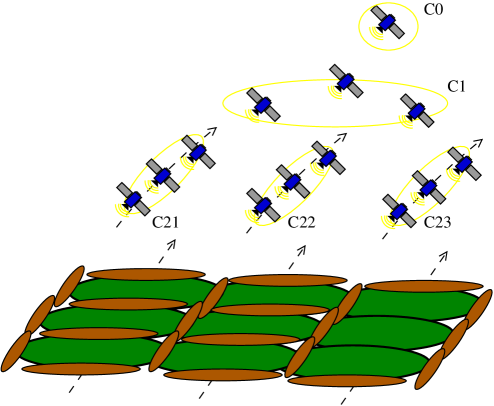
Figure 6: Three tiers of satellite constellations denoted as C0, C1 and C2x, and the corresponding moving ground footprints with overlapping (brown color) and non-overlapping (green color) regions.

Since architectures of existing cellular networks are well understood, equivalent solutions can be considered also for communication networks comprising the terrestrial and satellite segments. In particular, satellites can act as base stations for the terrestrial users who are mobile with respect to the satellites. However, as satellites are getting smaller to reduce the infrastructure costs, such satellites have limited power supply and small antennas, and cannot provide sufficiently strong signals to all ground users in the area. Thus, small satellite designs constrain the number of ground users being able to directly connect to the same satellite at the same time. These issues can be overcome by aggregating traffic of terrestrial users using a relatively small number of terminal stations on the ground. These ground stations act as base stations and interconnect mobile users on the ground with moving satellites. More importantly, the ground stations can exploit large antenna arrays with beamforming to simultaneously track one or more satellites in the sky, and they can implement other techniques developed previously for cellular systems such as coordinated multi-point transmissions to improve the reliability of communication links to satellites. Moreover, since terrestrial transmissions are likely to be cheaper than the transmissions via satellite relays, the key communication service provided by the satellite relays is to interconnect otherwise isolated sub-networks, especially if such terrestrial connections would be difficult to implement. Figure 7 shows the satellite communication bridge connecting two mutually isolated autonomous systems separated by the high mountains, the sea, or other such natural obstacles where using satellites may be the only viable option. Future work may assume constellation design for the ground stations as a counterpart of satellite constellations, especially with large MRE values due to antenna radiation patterns.

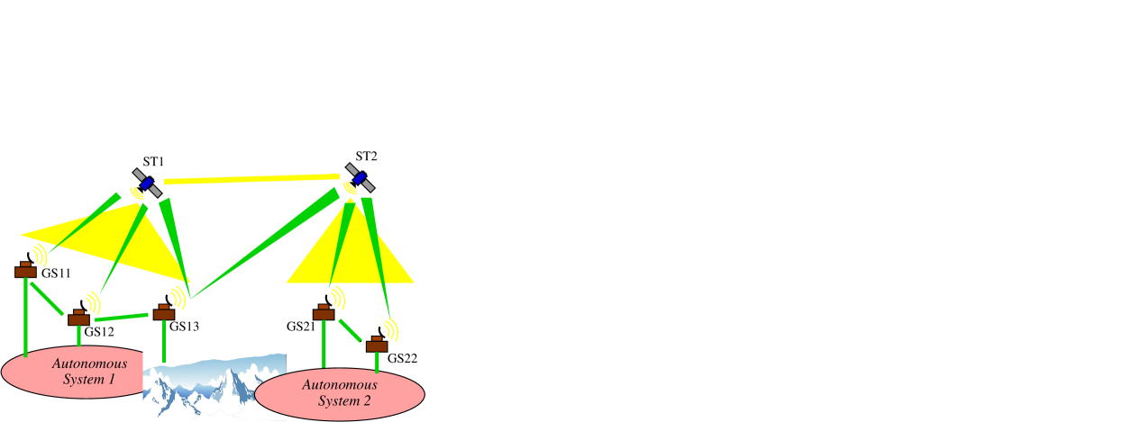
Figure 7: The satellite communication bridge interconnecting two autonomous systems separated by the natural obstacle (e.g., mountains, sea), so the terrestrial connection between the ground stations (GS) in different autonomous systems would be too expensive or too difficult.

References

It should be noted that the following resources on Wikipedia are summarized here mainly for the convenience. For more rigorous understanding of orbital mechanics, the interested reader is referred to classical textbooks on this topic, for example, Chobotov (2002) and Vallado and McClain (1997) cited above.

Wikipedia references

References

- Crisp et al. (2015) Crisp, N.; Smith, K.; Hollingsworth, P. Launch and deployment of distributed small satellite systems. Acta Astronautica 2015, 114, 65–78.
- Khan (2016) Khan, F. Multi-Comm-Core Architecture for Terabit-per-Second Wireless. IEEE Communications. Magazine 2016, 54, 124–129.
- Lee and Park (2019) Lee, K.H.; Park, K.Y. Overall Design of Satellite Networks for Internet Services with QoS Support. Electronics 2019, 8, 1–21.
- Wang et al. (2019) Wang, C.; Wang, H.; Wang, W. A Two-Hops State-Aware Routing Strategy Based on Deep Reinforcement Learning for LEO Satellite Networks. Electronics 2019, 8, 1–17.
- Clifford et al. (1994–2002) Clifford, N.; Pontieu, B.D.; Hunt, J. Visual Satellite Observer. http://www.satobs.org/.
- Zantou et al. (2005) Zantou, E.B.; Kherras, A.; Addaim, A. Orbit Calculation and Doppler Correction Algorithm in a LEO Satellite Small Ground Terminal. 19th Annual AIAA/USU Conference on Small Satellites, 2005, pp. 1–8.
- Chobotov (2002) Chobotov, V.A. Orbital Mechanics, 3rd ed. ed.; AIAA, 2002.
- Vallado and McClain (1997) Vallado, D.A.; McClain, W.D. Fundamentals and Astrodynamics and Applications, 1st ed. ed.; McGraw Hill, 1997.
- Bowman and Storz (2003) Bowman, B.R.; Storz, M.F. High accuracy satellite drag model (HASDM) review. American Astronautical Society 2003, 03-625, 1–10.
- Gergely (2015) Gergely, L.A. Celestial mechanics: The perturbed Kepler problem. Technical report, Univ. of Szeged, 2015.
- Capderou (2005) Capderou, M. Satellites Orbits and Missions; Springer, 2005.
- Ballard (1980) Ballard, A. Rosette Constellations of Earth Satellites. IEEE Transactions on Aerospace and Electronic Systems 1980, AES-16, 656–673.
- Danesfahani and Pirhadi (2006) Danesfahani, R.; Pirhadi, M. A Novel Constellation of Satellites. ICICT, 2006, pp. 2491–2495.
- Werner et al. (1995) Werner, M.; Jahn, A.; Lutz, E.; Böttcher, A. Analysis of System Parameters for LEO/ICO-Satellite Communication Networks. IEEE Journal on Selected Areas in Communications 1995, 13, 371–381.
- Chen et al. (2017) Chen, X.; Dai, G.; Reinelt, G.; Wang, M. A Semi-Analytical Method for Periodic Earth Coverage Satellites Optimization. IEEE Communications Letters 2017, 22, 534–537.
- Rec. ITU-R S.1257 (1997) Rec. ITU-R S.1257. Analytical Method To Calculate Visibility Statistics For Non-Geostationary Satellite Orbit Satellites As Seen From A Point On The Earth’s Surface. Technical report, ITU, 1997.
- Lyras et al. (2018) Lyras, N.K.; Efrem, C.N.; Kourogiorgas, C.I.; Panagopoulos, A.D. Optimum Monthly-Based Selection of Ground Stations for Optical Satellite Networks. IEEE Communications Letters 2018, 22, 1192–1195.
- Ali et al. (1999) Ali, I.; Al-Dhahir, N.; Hershey, J.E. Predicting the Visibility of LEO Satellites. IEEE Transactions on Aerospace and Electronic Systems 1999, 35, 1183–1190.
- Ali et al. (1998) Ali, I.; Al-Dhahir, N.; Hershey, J.E. Doppler Characterization for LEO Satellites. IEEE Transactions on Communications 1998, 46, 309–313.
- Pratt et al. (1999) Pratt, S.R.; Raines, R.A.; Fossa Jr., C.E.; Temple, M.A. An Operational and Performance Overview of the Iridium Low Earth Orbit Satellite Systems. IEEE Communication Surveys and Tutorials 1999, 2, 2–10.
- Cakaj et al. (2014) Cakaj, S.; Kamo, B.; Lala, A.; Rakipi, A. The Coverage Analysis for Low Earth Orbiting Satellites at Low Elevation. International Journal of Advanced Computer Science and Applications 2014, 5, 6–10.
- Seyedi and Safavi (2012) Seyedi, Y.; Safavi, S.M. On the Analysis of Random Coverage Time in Mobile LEO Satellite Communications. IEEE Communications Letters 2012, 16, 612–615.
- Hossain et al. (2017) Hossain, M.S.; Hassan, S.S.; Atiquzzaman, M.; Ivancic, W. Survivability and scalability of space networks: a survey. Telecommunication Systems 2017. doi:\changeurlcolorblack10.1007/s11235-017-0396-y.
- Lutz et al. (1991) Lutz, E.; Cygan, D.; Dippold, M.; Dolainsky, F.; Papke, W. The Land Mobile Satellite Communication Channel-Recording, Statistics, and Channel Model. IEEE Transactions on Vehicular Technology 1991, 40, 375–386.
- Abdi et al. (2003) Abdi, A.; Lau, W.C.; Alouini, M.S.; Kaveh, M. A New Simple Model for Land Mobile Satellite Channels: First- and Second-Order Statistics. IEEE Transactions on Communications 2003, 2, 519–528.

References

- (1) Wikipedia contributors, “Angular momentum,” Wikipedia, The Free Encyclopedia, https://en.wikipedia.org/w/index.php?title=Angular_momentum (accessed September 17, 2019).
- (2) Wikipedia contributors, “Argument of periapsis,” Wikipedia, The Free Encyclopedia, https://en.wikipedia.org/w/index.php?title=Argument_of_periapsis (accessed September 17, 2019).
- (3) Wikipedia contributors, “Earth-centered, Earth-fixed,” Wikipedia, The Free Encyclopedia, https://en.wikipedia.org/w/index.php?title=ECEF (accessed September 17, 2019).
- (4) Wikipedia contributors, “Earth-centered inertial,” Wikipedia, The Free Encyclopedia, https://en.wikipedia.org/w/index.php?title=Earth-centered_inertial (accessed September 17, 2019).
- (5) Wikipedia contributors, “Earth radius,” Wikipedia, The Free Encyclopedia, https://en.wikipedia.org/w/index.php?title=Earth_radius (accessed September 17, 2019).
- (6) Wikipedia contributors, “Earth’s rotation,” Wikipedia, The Free Encyclopedia, https://en.wikipedia.org/w/index.php?title=Earth%27s_rotation (accessed September 17, 2019).
- (7) Wikipedia contributors, “Eccentric anomaly,” Wikipedia, The Free Encyclopedia, https://en.wikipedia.org/w/index.php?title=Eccentric_anomaly (accessed September 17, 2019).
- (8) Wikipedia contributors, “Eccentricity vector,” Wikipedia, The Free Encyclopedia, https://en.wikipedia.org/w/index.php?title=Eccentricity_vector (accessed September 17, 2019).
- (9) Wikipedia contributors, “Kepler’s laws of planetary motion,” Wikipedia, The Free Encyclopedia, https://en.wikipedia.org/w/index.php?title=Kepler%27s_laws_of_planetary_motion (accessed September 17, 2019).
- (10) Wikipedia contributors, “Longitude of the ascending node,” Wikipedia, The Free Encyclopedia, https://en.wikipedia.org/w/index.php?title=Longitude_of_the_ascending_node (accessed September 17, 2019).
- (11) Wikipedia contributors, “Mean anomaly,” Wikipedia, The Free Encyclopedia, https://en.wikipedia.org/w/index.php?title=Mean_anomaly (accessed September 17, 2019).
- (12) Wikipedia contributors, “Mean motion,” Wikipedia, The Free Encyclopedia, https://en.wikipedia.org/w/index.php?title=Mean_motion (accessed September 17, 2019).
- (13) Wikipedia contributors, “Newton’s method,” Wikipedia, The Free Encyclopedia, https://en.wikipedia.org/w/index.php?title=Newton%27s_method (accessed September 17, 2019).
- (14) Wikipedia contributors, “Orbital eccentricity,” Wikipedia, The Free Encyclopedia, https://en.wikipedia.org/w/index.php?title=Orbital_eccentricity (accessed September 17, 2019).
- (15) Wikipedia contributors, “Orbital inclination,” Wikipedia, The Free Encyclopedia, https://en.wikipedia.org/w/index.php?title=Orbital_inclination (accessed September 17, 2019).
- (16) Wikipedia contributors, “Semi-major and semi-minor axes,” Wikipedia, The Free Encyclopedia, https://en.wikipedia.org/w/index.php?title=Semi-major_and_semi-minor_axes (accessed September 17, 2019).
- (17) Wikipedia contributors, “Sidereal time,” Wikipedia, The Free Encyclopedia, https://en.wikipedia.org/w/index.php?title=Sidereal_time (accessed September 17, 2019).
- (18) Wikipedia contributors, “Standard gravitational parameter,” Wikipedia, The Free Encyclopedia, https://en.wikipedia.org/w/index.php?title=Standard_gravitational_parameter (accessed September 17, 2019).
- (19) Wikipedia contributors, “True anomaly,” Wikipedia, The Free Encyclopedia, https://en.wikipedia.org/w/index.php?title=True_anomaly (accessed September 17, 2019).
- (20) Wikipedia contributors, “Vis-viva equation,” Wikipedia, The Free Encyclopedia, https://en.wikipedia.org/w/index.php?title=Vis-viva_equation (accessed September 17, 2019).