Spectral properties of quasars from Sloan Digital Sky Survey data release 14: The catalog

Abstract

We present measurements of the spectral properties for a total of 526,265 quasars, out of which 63% have continuum S/N$>3$ pixel^-1, selected from the fourteenth data release of the Sloan Digital Sky Survey (SDSS-DR14) quasar catalog. We performed a careful and homogeneous analysis of the SDSS spectra of these sources, to estimate the continuum and line properties of several emission lines such as H${\alpha}$, H${\beta}$, H${\gamma}$, Mg ii, C iii], C iv and Ly${\alpha}$. From the derived emission line parameters, we estimated single-epoch virial black hole masses ($M_{\mathrm{BH}}$) for the sample using H${\beta}$, Mg ii and C iv emission lines. The sample covers a wide range in bolometric luminosity ($\log L_{\mathrm{bol}}$; erg s^-1) between 44.4 and 47.3 and $\log M_{\mathrm{BH}}$ between 7.1 and 9.9 $M_{\odot}$. Using the ratio of $L_{\mathrm{bol}}$ to the Eddington luminosity as a measure of the accretion rate, the logarithm of the accretion rate is found to be in the range between $-$2.06 and 0.43. We performed several correlation analyses between different emission line parameters and found them to match with that known earlier using smaller samples. We noticed that strong Fe ii sources with large Balmer line width, and highly accreting sources with large $M_{\mathrm{BH}}$ are rare in our sample. We make available online an extended and complete catalog that contains various spectral properties of 526,265 quasars derived in this work along with other properties culled from the SDSS-DR14 quasar catalog.

=1

1 Introduction

Quasars, a class of active galactic nuclei (AGN), are powered by accretion of matter onto a super massive black hole surrounded by an accretion disk (e.g. Antonucci, 1993). The availability of a large number of quasars with measured line and continuum properties is of paramount importance in a wide variety of astrophysical research such as galaxy evolution, black hole growth, etc. For example, the mass of the black holes ($M_{\mathrm{BH}}$) in AGN is found to be strongly correlated with host galaxies velocity dispersion suggesting the co-evolution of the black hole and host galaxy (e.g., Kormendy & Ho, 2013). Thus, measuring $M_{\mathrm{BH}}$ for a large sample of quasars is required to study the growth and evolution of black hole across cosmic time. A direct method to measure $M_{\mathrm{BH}}$ in quasars over a large range of redshifts is via the technique of reverberation mapping (Blandford & McKee, 1982; Peterson, 1993) and such studies show a strong correlation between the quasar monochromatic luminosity ($L$) at 5100 Å  and the size ($R$) of the broad line region (BLR; e.g., Kaspi et al., 2000; Bentz et al., 2009, 2013). Since reverberation mapping requires long-term monitoring campaign, which is difficult for high redshift and high luminosity objects, the size-luminosity ($R-L$) relation has been used to estimate $M_{\mathrm{BH}}$ from the single-epoch spectrum for which monochromatic luminosity and emission line width measurements are available (e.g., Woo & Urry, 2002; Shen et al., 2011). The values of $M_{\mathrm{BH}}$ estimated from single-epoch spectrum are mostly consistent with the reverberation mapping $M_{\mathrm{BH}}$ estimates within a factor of few (e.g., Wandel et al. 1999; Vestergaard 2002; McLure & Jarvis 2002; Grier et al. 2017 but also see Vestergaard & Peterson 2006, Shen 2013 and Peterson 2014 for merits and caveats of single-epoch $M_{\mathrm{BH}}$).

Also, statistical studies of quasars will help in a better understanding of quasar properties (Urry & Padovani, 1995; Kellermann et al., 1989) such as the quasar luminosity function (Richards et al., 2006b), black hole mass function, which shows a peak at $z\sim 2$ (Vestergaard & Osmer, 2009; Kelly et al., 2010), and the Eddington ratio distribution, which peaks at $L_{\mathrm{bol}}/L_{\mathrm{Edd}}\sim 0.05$ (Kelly et al., 2010), where, $L_{\mathrm{bol}}$ is the bolometric luminosity and $L_{\mathrm{Edd}}=1.3\times 10^{38}$ ($M_{\mathrm{BH}}$/$M_{\odot}$) erg s^-1 is the Eddington luminosity. Several correlations between continuum and emission line properties in quasars are available, e.g., the anti-correlation between line equivalent width (EW) and continuum luminosity (Baldwin, 1977), especially strong in C iv and Mg ii lines (Shen et al., 2011), correlations between continuum luminosity and line widths and luminosities, etc. (e.g., Boroson & Green, 1992; Greene & Ho, 2005; Shen et al., 2011; Rakshit et al., 2017; Calderone et al., 2017). Also, studies of the emission lines from AGN will help in enhancing our understanding of the physical conditions of the gas close to the central regions of AGN (Osterbrock, 1989).

All of the above studies require large samples of quasars. Since the discovery of quasars about more than half a century ago (Schmidt, 1963), the number of quasars that are known has increased gradually. A significant increase in the number of quasars happened in the last two decades with the bulk of the contribution coming from the Sloan Digital Sky Survey (SDSS; York et al., 2000). In addition to SDSS, other surveys too have contributed to the increase in the number of quasars such as the 2dF quasar redshift survey (2QZ; Croom et al., 2004), the bright quasar survey (Schmidt & Green, 1983) and the large bright quasar survey (LBQS; Hewett et al. 1995). Also, the number of quasars is expected to increase manifold in the future from the next generation large optical imaging survey using the Large Synoptic Survey Telescope (LSST, now known as Vera C. Rubin Observatory; Ivezić et al., 2019, 2014).

Among the many available quasar surveys, SDSS has provided us with the largest homogeneous sample of quasars with optical spectra. Each SDSS quasar survey had different science goals. For example SDSS DR7 quasar catalog (Schneider et al., 2010) consists of 105,783 spectroscopically confirmed quasars from SDSS-I/II survey (York et al., 2000) whose aim was to study quasar luminosity function (e.g. Richards et al., 2006b) and clustering properties (e.g. Hennawi et al., 2006; Shen et al., 2007). The survey also led to the discovery of many high redshift $z\sim 6$ quasars (e.g., Fan et al., 2006; Jiang et al., 2008), and broad absorption line quasars (e.g., Reichard et al., 2003; Trump et al., 2006; Gibson et al., 2008). The SDSS-III/BOSS survey (Eisenstein et al., 2011; Dawson et al., 2013) was intended to discover a large sample of quasars with Lyman-$\alpha$ forest, which fall in the redshift range of $2.15-3.5$ to constrain the Baryon Acoustic Oscillation (BAO) scale. This survey lead to the discovery of 270,000 quasars, mostly at $z>2$, which helped to provide strong cosmological constraints at z$\sim 2.5$ through the auto-correlation of Lyman-$\alpha$ forest (e.g. Bautista et al., 2017) and cross-correlation of quasars and Lyman-$\alpha$ forest (e.g., du Mas des Bourboux et al., 2017).

The SDSS-IV has multiple goals, SDSS-IV/eBOSS (see Dawson et al., 2016) is dedicated to measure percent-level angular diameter distance $d_{A}$(z) and Hubble parameter H(z) using 250,000 new spectroscopically confirmed luminous red galaxies, 195,000 new emission line galaxies, 500,000 spectroscopically confirmed quasars and 60,000 new Lyman-$\alpha$ forest quasar measurements at redshifts $z>2.1$. The time-domain Spectroscopic Survey (TDSS) of SDSS-IV was designed to study the spectroscopic variability of quasars, and the Spectroscopic Identification of eROSITA Sources (SPIDERS) program was designed to investigate X-ray sources in SDSS-IV. Pâris et al. (2018) recently compiled a quasar catalog from SDSS-IV including all previously spectroscopically selected quasars from SDSS I, II and III surveys. This catalog consists of 526,356 quasars over 9376 degree² region of the sky from SDSS with 144,046 newly discovered quasars from SDSS-IV. The catalog of Pâris et al. (2018) is, therefore, a unique and the largest list of spectroscopically confirmed quasars selected homogeneously and covering a large part of the northern sky. Once all the spectral properties of the quasars in Pâris et al. (2018) are available, the catalog can serve as the largest quasar database useful to address a wide variety of astrophysical problems and/or revisit the correlations already known between various quasar properties.

The spectral properties of SDSS DR7 quasars have been studied by Shen et al. (2011, hereafter S11), consisting of about 100,000 quasars. Calderone et al. (2017, hereafter C17) studied spectral properties of about 70,000 quasars at $z<2$ from SDSS-DR10 (Ahn et al., 2014), which contains the first data release from SDSS-III. The latest SDSS-DR14 quasar catalog of Pâris et al. (2018) not only increases the number of quasars by a factor of 5 compared to SDSS DR7, it also covers about 1.5 mag fainter sources ($i$-band absolute magnitude M${}_{i}(z=2)<-20.5$) than SDSS DR7 (M${}_{i}(z=2)<-22$). As the DR14 quasar catalog includes much fainter quasars, this opens up the possibility of the exploration of the properties of quasars over a large range in luminosity. Though the catalog contains the X-ray, UV, optical, IR and radio imaging properties of the quasars wherever available, it lacks spectral information of the sources. About 332,000 ($\sim$ 63%) sources in DR14 catalog have the continuum S/N$>3$ pixel^-1. This is a factor of 3 larger than the entire sample of S11 catalog. Thus, DR14 catalog with spectral information will be useful for the astronomical community not only for statistical studies of quasars but also to discover and investigate peculiar objects.

We, therefore, carried out detailed spectral modeling of all the quasars cataloged in Pâris et al. (2018) and provide a new catalog of continuum and emission line properties of 526,265 quasars along with $M_{\mathrm{BH}}$ and Eddington ratio. This paper is structured as follows. Our data and spectral analysis procedures are described in section 2. We compare our measurements with the previous works in section 3. In section 4, we discuss the impact of the S/N of the spectra on the derived spectral quantities. We discuss some applications of the catalog in section 5 with a summary in section 6. In Appendix A we define and describe the quality of our spectral measurements and in Appendix B we present the spectral catalog. A cosmology with $H_{0}=70\,\mathrm{km\,s^{-1}\,Mpc^{-1}}$, $\Omega_{\mathrm{m}}=0.3$, and $\Omega_{\lambda}=0.7$ is assumed throughout.

2 Data and spectral analysis

We started with the SDSS DR14 quasar catalog (version “DR14Q$\_$v4$\_$4”) by Pâris et al. (2018, hereafter DR14Q), which includes all the spectroscopically confirmed quasars observed during any SDSS data release, consisting of 526,356 quasars based on $i$-band absolute magnitude M${}_{i}(z=2)<-20.5$ and having at least one emission line with full width at half maximum (FWHM) larger than 500 km$s^{-1}$ or having interesting/complex absorption features. It was constructed from SDSS-DR14 (Abolfathi et al., 2018) and a major part of the newly discovered quasars in DR14Q are from the extended Baryon Oscillation Spectroscopic Survey (eBOSS) of SDSS IV (Myers et al., 2015). A detailed description of DR14Q can be found in Pâris et al. (2018).

To measure the spectral information of the quasars in DR14Q, we first downloaded all the processed and calibrated spectra from the SDSS database. We then analysed each spectrum using the publicly available multi-component spectral fitting code PyQSOFit developed by Guo et al. (2018). A detailed description of the code and its applications can be found in Guo et al. (2019) and Shen et al. (2019). First, we corrected each spectrum for Galactic extinction using the Schlegel et al. (1998) map and a Milky Way extinction law of Fitzpatrick (1999) with $R_{V}=3.1$. We then transformed the observed spectrum to the rest frame wavelength using the redshift ($z$) value provided in DR14Q. Finally, we performed multi-component spectral fittings to each spectrum.

Table 1: Emission line fitting parameters. The columns are as follows (1) name of the line complex, (2) wavelength range (in Å) of the line fitting window, (3) name of the emission line and (4) number of Gaussian used in the fitting.

Complex name	wavelength range	emission line name	Number of Gaussian
	(Å)
(1)	(2)	(3)	(4)
H$\alpha$	6400-6800	H$\alpha$ broad	3
		H$\alpha$ narrow	1
		[N ii]6549	1
		[N ii]6585	1
		[S ii]6718	1
		[S ii]6732	1
H$\beta$	4640-5100	H$\beta$ broad	3
		H$\beta$ narrow	1
		[O iii]4959 core	1
		[O iii]4959 wing	1
		[O iii]5007 core	1
		[O iii]5007 wing	1
H$\gamma$	4250-4440	H$\gamma$ broad	1
		H$\gamma$ narrow	1
		[O iii]4364	1
Mg ii	2700-2900	Mg ii broad	2
		Mg ii narrow	1
C iii]	1850-1970	C iii]	2
C iv	1500-1600	C iv	3
Ly$\alpha$	1150-1290	Ly$\alpha$	3
		N v 1240	1

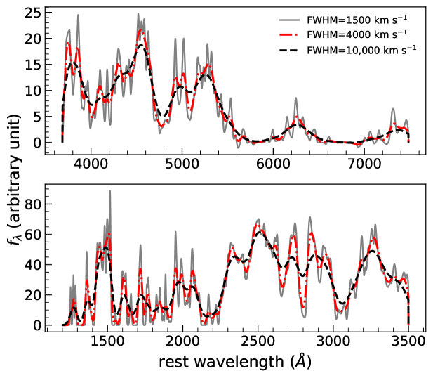
Figure 1: Examples of iron template broadened by the convolution of a Gaussian of different FWHM (parameter $b1$ in equation 3). The upper panel is the optical Fe II from Boroson & Green (1992) and lower panel is the UV Fe II built by Shen et al. (2019) from the templates of Vestergaard & Wilkes (2001), Tsuzuki et al. (2006) and Salviander et al. (2007).

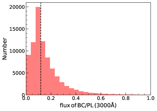
Figure 2: The distribution of flux ratio of Balmer continuum to power-law at 3000 Å  for $z<1.1$. The dashed line represents the median of the distribution.

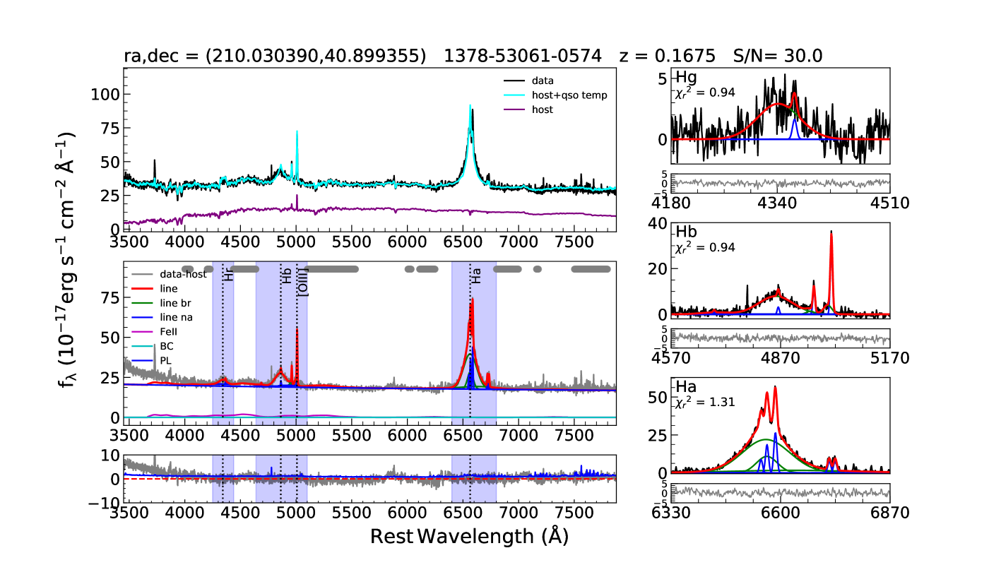
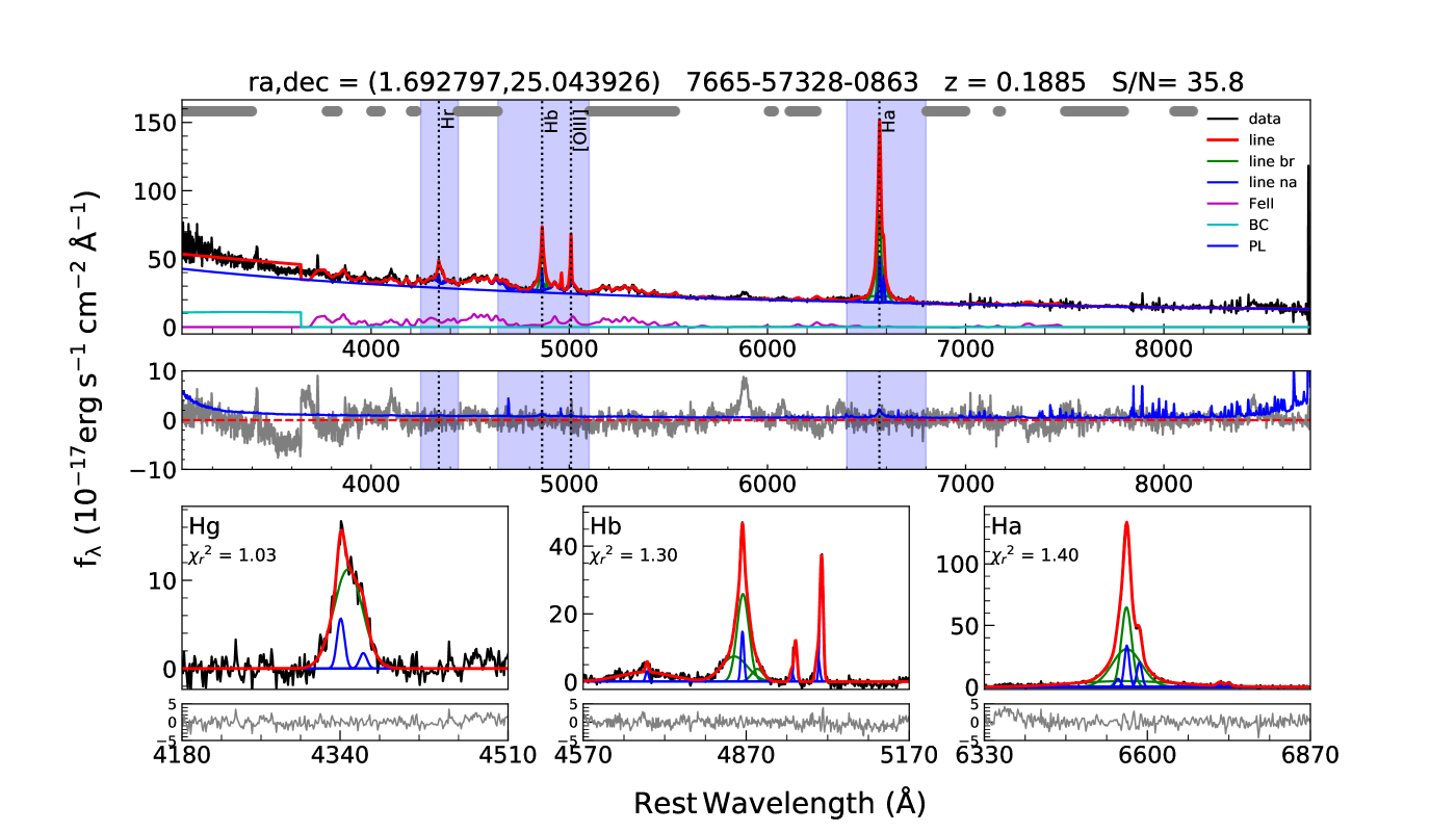
Figure 3: Examples of spectral decomposition. Top: an example of a quasar spectrum with significant host galaxy contribution. Upper subplot: SDSS data (black), the best fit quasar+host galaxy template (cyan) and the decomposed host galaxy (purple). Middle subplot: The host subtracted spectrum (gray), the power-law (blue), Fe II (magenta), broad line (green), narrow line (blue) and the total best fit model (red), which is a sum of $f_{\mathrm{cont}}$+line are shown. The wavelength windows used to fit AGN continuum is also shown at the top (bar). Bottom subplot: The residual (gray) in the unit of error spectrum i.e., (data-model)/error, is shown along with error spectrum (blue). Bottom: An example of a quasar spectrum without significant host galaxy contribution. Upper subplot: the power-law (blue), Fe ii (magenta), broad line (green), narrow line (blue) and the total best fit model (red), which is a sum of $f_{\mathrm{cont}}$+line are shown in each panel. Middle plot: residual (gray) in the unit of error spectrum (blue). A zoomed version of individual line complex is also shown along with the residual in the unit of error spectrum. The shaded region shows the wavelength window at which each line complex was fitted (see Table 1) and the reduced $\chi^{2}$ obtained for each of the line complex. The median continuum S/N per pixel is also given.

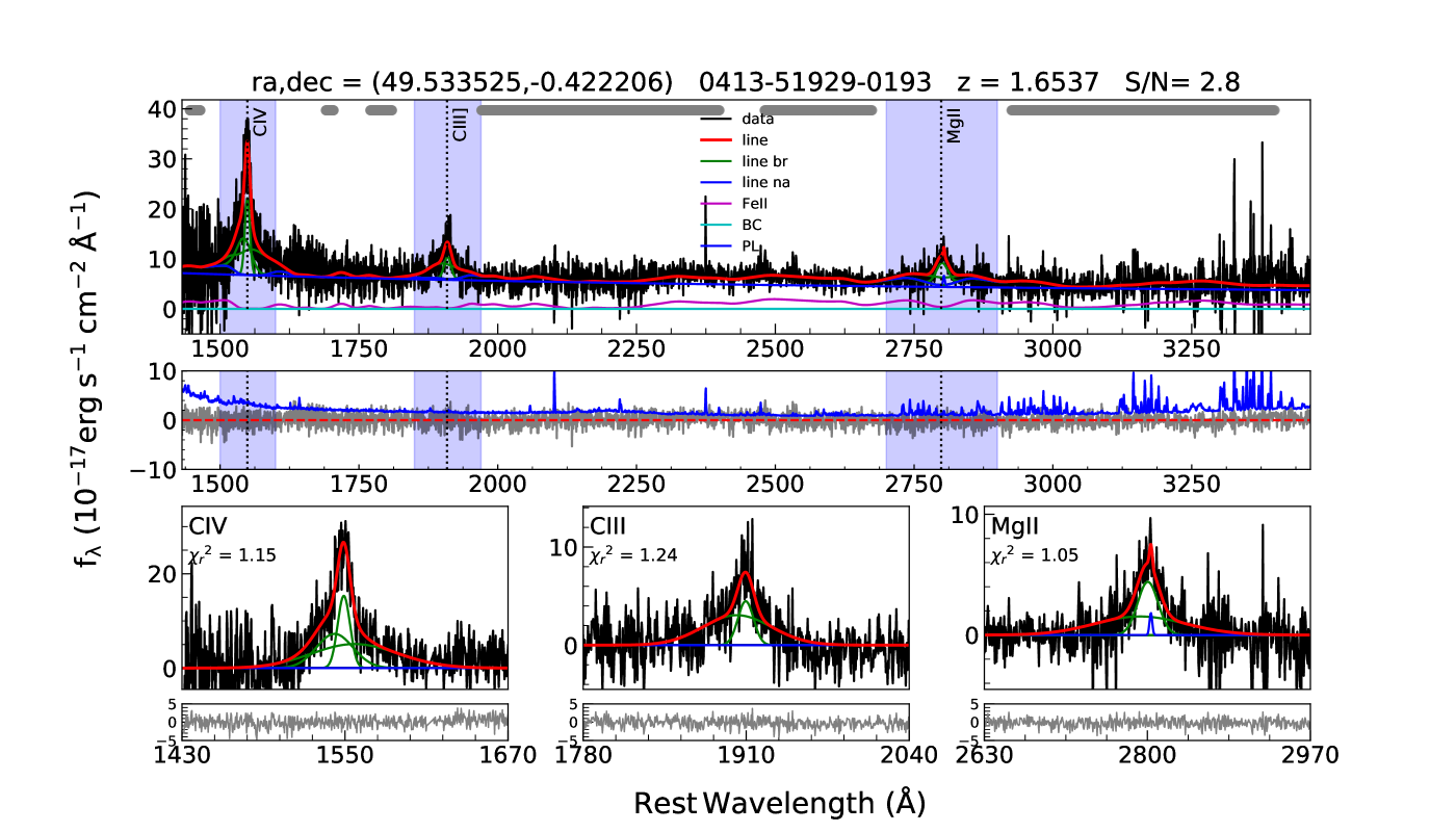
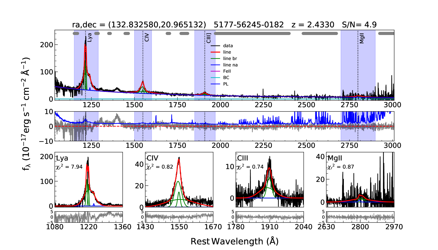
Figure 4: Example of spectral decomposition for poor continuum S/N spectra. Labels are same as in Figure 3.

2.1 Continuum components

The light from stars in the host-galaxy of a quasar can contribute to the observed quasar’s spectrum, particularly significant for low-z quasars ($z<0.8$). Thus, to extract intrinsic AGN properties, the host galaxy contribution to each spectrum must be removed. We, therefore, carried out host galaxy-quasar decomposition to the spectra for $z<0.8$ quasars based on the principal component analysis (PCA; Yip et al., 2004a, b) implemented in PyQSOFit code. The PCA method has been used in several previous studies (Vanden Berk et al., 2006; Shen et al., 2008a, 2015) to decompose host galaxy and quasar contribution assuming that the observed composite spectrum is a combination of two independent sets of eigenspectra taken from pure galaxy (Yip et al., 2004a) and pure quasar (Yip et al., 2004b) samples. The first three galaxy eigenspectra contain 98% of the galaxy sample information while the first ten quasar eigenspectra contain 92% of the quasar sample information. Vanden Berk et al. (2006) performed PCA on 11,000 SDSS quasars. They also studied the reliability of spectral decomposition with signal-to-noise ratio (S/N) of the spectrum, host galaxy fraction, galaxy class, etc. The host galaxy decomposition is considered to be successful if the host galaxy fraction in the wavelength range of 4160-4210Å  is larger than 10%. This method also has been applied by Shen et al. (2008a, 2015) to decompose the host galaxy from the SDSS spectra. Here too, we applied PCA to decompose the host-galaxy contribution using 5 PCA components for galaxies that can reproduce about 98% of the galaxy sample and 20 PCA components for quasars that can reproduce about 96% of the quasar sample and the global model (independent of redshift and luminosity). We then subtracted the host contribution, if present, from each spectrum.

Using the host-galaxy subtracted spectrum, we modeled the entire continuum, masking the prominent emission lines as

$$f_{\mathrm{cont}}=f_{\mathrm{pl}}+f_{\mathrm{BC}}+f_{\mathrm{FeII}}$$ (1)

where the power-law continuum ($f_{\mathrm{pl}}$) is

$$f_{\mathrm{pl}}=\beta\big{(}\lambda/\lambda_{0}\big{)}^{\alpha},$$ (2)

with a reference wavelength $\lambda_{0}=3000\AA$. The parameters $\alpha$ and $\beta$ are the power-law slope and normalization parameter, respectively.

The Fe ii model ($f_{\mathrm{Fe\,\textsc{ii}}}$) is

$$f_{\mathrm{Fe\,\textsc{ii}}}=b_{0}\,F_{\mathrm{Fe\,\textsc{ii}}}(\lambda,b1,b2),$$ (3)

where the parameters $b_{0}$, $b1$, $b2$ are the normalization, the Gaussian FWHM used to convolve the Fe II template, and the wavelength shift applied to the Fe II template, respectively, to fit the data. Both the UV and optical Fe II emission were modeled. In PyQSOFit, the UV Fe II template is a modified template built by Shen et al. (2019) with constant velocity dispersion of 103.6 km s^-1 from the templates of Vestergaard & Wilkes (2001), Tsuzuki et al. (2006) and Salviander et al. (2007). For the wavelength range of $1000-2200$Å  the template is from Vestergaard & Wilkes (2001), for $2200-3090$Å  the template is from Salviander et al. (2007) which extrapolates the Fe II flux underneath the Mg II line and for $3090-3500$Å  the template is from Tsuzuki et al. (2006). The optical Fe ii template (3686$-$7484 Å ) is based on Boroson & Green (1992). To model the Fe II emission for each of our spectra, we first convolved the template with the parameter $b1$ which is constrained in the range of 1200-10,000 km s^-1 with an initial guess of 3000 km s^-1. A small wavelength shift ($b2$), constrained to be within 1% of the template wavelength was also applied to fit the data. Then the parameters $b_{0}$, $b1$, and $b2$ were varied within the range mentioned above until the best fit model which represents the data was found. In Figure 1, we show examples of template broadening for different values of Gaussian FWHM ($b1$).

The Balmer continuum ($f_{\mathrm{BC}}$; Grandi, 1982; Dietrich et al., 2002) is defined as

$$f_{\mathrm{BC}}=F_{\mathrm{BE}}B_{\lambda}(T_{\mathrm{e}})\big{(}1-e^{-\tau_{\lambda}(\lambda/\lambda_{\mathrm{BE}})^{3}}\big{)}$$ (4)

where $F_{\mathrm{BE}}$ is the normalized flux density, $\tau_{\lambda}$ is the optical depth at the Balmer edge of wavelength $\lambda_{\mathrm{BE}}=3646$Å, $B_{\lambda}(T_{\mathrm{e}})$ is the Planck function at the electron temperature $T_{e}$. As many low-z objects do not have enough spectral coverage to fit a Balmer component, it is fitted whenever the continuum window has at least 100 pixels below $\lambda_{\mathrm{BE}}$. We used $F_{\mathrm{BE}}$ as a free parameter keeping $T_{e}=15,000$ K, and $\tau_{\lambda}=1$ fixed to avoid degeneracy between the parameters following Dietrich et al. (2002) and C17. Moreover, for sources with $z>1.1$, the Balmer component resembles a simple power-law. Thus, following previous studies (e.g., C17), we further allowed $F_{\mathrm{BE}}$ to vary between 0 and $0.1\times F_{3675}$. Here $F_{3675}$ is the flux density at $\lambda=3675$Å, where the Fe II contribution is insignificant. The upper limit is also justified from the distribution of flux ratio of Balmer to power-law continuum at 3000Å  (see Figure 2) for $z<1.1$ sources, which has a median of $\sim$0.1.

We noticed that in a few low-z ($z<0.3$) objects the blue part of the spectrum between $3000-4000$ Å is much steeper and the entire continuum cannot be well-fitted with a power-law and Balmer component. For those objects, we limited the spectral fitting range to above 4000Å, thereby excluding the steep rise towards the UV.

Many high-z spectra were affected by broad and narrow absorption lines that could bias the line fitting results, hence, we used ‘rej_abs = True’ option in PyQSOFit to reduce this bias. The code first performed continuum modeling (‘tmp_cont’) of the spectrum and removed the 3$\sigma$ (where $\sigma$ is the flux uncertainty) outliers below the continuum (i.e., pixels where flux $<$ tmp_cont $-$3 $\times$ flux uncertainty) for wavelength $<3500$Å  and then performed a second iteration of continuum model fit to the 10 pixels box-car smoothed spectrum excluding the outliers. Such a method is found to be useful to reduce the impact of absorption features as noted in Shen et al. (2011, 2019).

2.2 Emission line components

The best fit continuum model was subtracted from each spectrum leading to only the line spectrum. Individual line complex was fitted separately, while all the emission lines within a line complex were fitted together. The full list of emission lines and the number of Gaussian components used for the individual line are given in Table 1. Broad emission line profiles in many objects can be very complex (e.g., double-peaked, flat top, asymmetric) and can not be well represented by a single Gaussian. Moreover, the line width estimated by a single Gaussian model is systematically larger by 0.1 dex compared to the multiple Gaussian model (Shen et al., 2008b, 2011). Thus, following previous studies, we used multiple Gaussians to model the broad emission line profiles (e.g., Greene & Ho, 2005; Shen et al., 2011). During the fitting, the velocity and width of all the narrow components in H$\beta$ and H$\alpha$ complex were tied together with an added constraint that the maximum allowed FWHM of narrow components is 900 km s^-1, while the broad components have FWHM $>900$ km s^-1. The FWHM criterion was adopted to separate Type 1 AGN from the Type 2 AGN following previous studies (e.g., Wang et al., 2009; Calderone et al., 2017; Wang et al., 2019; Coffey et al., 2019). The velocity offsets of the broad and narrow components were restricted to $\pm$3000 km s^-1 and $\pm$1000 km s^-1, respectively. Furthermore, the flux ratios of [O iii] and [N ii] doublets were fixed to their theoretical values, i.e., $F(5007)/F(4959)=3$ and $F(6585)/F(6549)=3$. Note that, we did not use any narrow component to model C iii] and C iv emission lines and the line FWHM and flux were determined from the whole line because of ambiguity in the presence of narrow components in these lines (also see Shen et al., 2011, 2019).

A few examples of the spectral decomposition are shown in Figures 3 and 4 for spectra of different qualities. The median continuum S/N (estimated from the rest-frame spectrum in the regions around 5100Å, 4210Å, 3000Å, 2245Å, and 1350Å  depending on the spectral coverage) is also noted in the Figure. Note that due to a large number of quasars, visual inspection of all the spectral fittings was not possible. Thus, only random checks of a few thousand spectra in various redshift and S/N bins were made. All the spectral fitting plots and individual model components are made publicly available for the users. We also provide various quality flags on the spectral quantities to access the reliability of the measurements. The good quality measurements are given a quality flag=0. Any measurements with quality flag $>0$, may not be reliable either due to poor S/N or bad spectral decomposition. Therefore, sources with flag $>0$ should be used cautiously. The criteria for fulfillment of each quality flag is defined and described in Appendix A including detailed statistics on each quality flag.

2.3 Spectral quantities

We measured the continuum (slope, luminosity) and emission line (line peak, FWHM, EW, luminosity, etc.) properties from the best fit model. Various studies (e.g., Collin et al., 2006; Rafiee & Hall, 2011) suggested that line dispersion ($\sigma_{\mathrm{line}}$) i.e., the second moment of the line (see Peterson et al., 2004) is a better measure of emission line width compared to FWHM. However, FWHM is less affected by the noise in the line wings and treatments of line blending (e.g., H$\beta$ blended with Fe II, He II$\lambda$4686 and [O III]) than the ${\sigma}_{\mathrm{line}}$. On the other hand, ${\sigma}_{\mathrm{line}}$ is less sensitive to the treatments of narrow component removal and peculiar line profiles. Instead of line dispersion, FWHM is preferred because of its easiness of the measurement and repeatability, especially in poor quality spectra where the line wings are difficult to constrain and ${\sigma}_{\mathrm{line}}$ can not be measured reliably. Despite that, following the prescription of Wang et al. (2019), we also measured ${\sigma}_{\mathrm{line}}$ for all the broad emission lines and included them in the catalog.

The uncertainty in each of the spectral quantities was estimated using Monte Carlo approach (e.g., Shen et al., 2011, 2019; Rakshit & Woo, 2018). We created a mock spectrum by adding to the original spectrum at each pixel a Gaussian random deviate with zero mean and $\sigma$ given by the flux uncertainty at that pixel. We then performed the same spectral fitting on the mock spectrum as was done for the original spectrum and estimated all the spectral quantities from the mock spectrum. We created 50 such mock spectra for each object allowing us to obtain the distribution of each spectral quantity. Finally, for each spectral quantity, semi-amplitude of the range enclosing the 16th and 84th percentiles of the distribution was taken as the uncertainty of that quantity. Therefore, all the uncertainties of the spectral quantities reported in this work were calculated using the Monte Carlo approach.

We calculated $L_{\mathrm{bol}}$ from the monochromatic luminosity using the bolometric correction factor given in S11 as adapted from the analysis in Richards et al. (2006a)

$$L_{\mathrm{bol}}=\begin{cases}9.26\times L_{5100},&\text{if }z<0.8\\ 5.15\times L_{3000},&\text{if }0.8\leq z<1.9\\ 3.81\times L_{1350},&\text{if }z\geq 1.9\end{cases}$$

Note that the above correction factors are derived from the mean spectral energy distribution of AGN and using a single value could lead to 50% uncertainty in $L_{\mathrm{bol}}$ measurements (Richards et al., 2006a). Estimating bolometric luminosity for individual source requires multi-band data from radio to X-ray to build spectral energy distribution, which is not available for most of the quasars. However, the bolometric correction factor allows us to estimate the bolometric luminosity from their monochromatic luminosity albeit with large uncertainty.

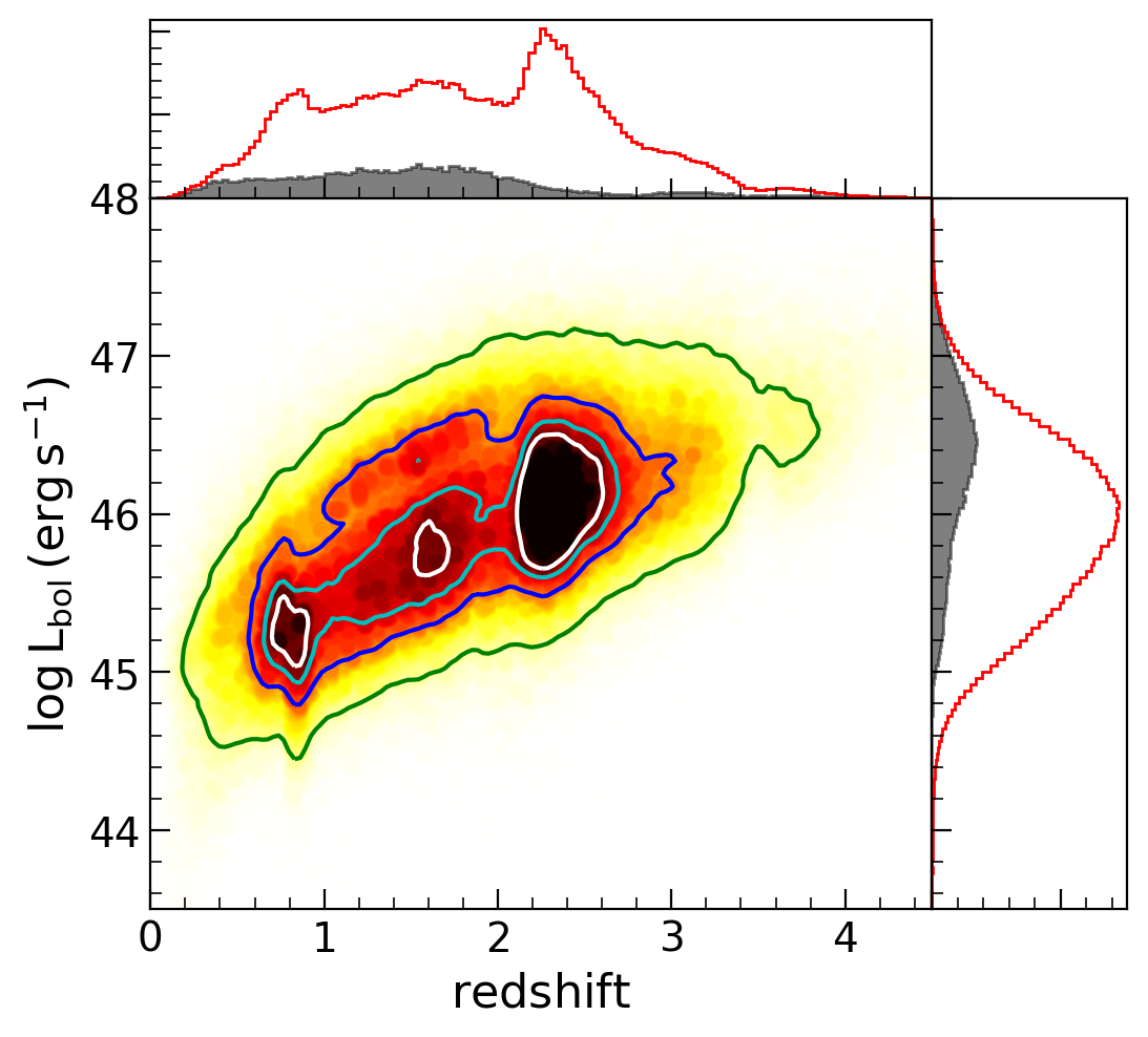
Figure 5: Bolometric luminosity vs. redshift. The 20, 40, 68 and 95 percentile density contours along with density maps are shown. The redshift and bolometric luminosity distributions are also shown for DR14 quasars sample (empty histogram, this work) along with DR7 quasars (filled histogram, S11). A large number of high redshift and low luminous quasars were targeted by DR14 compared to DR7.

In Figure 5, we plot $L_{\mathrm{bol}}$ against redshift for DR14 quasars. The DR7 quasars from S11 are also shown. As mentioned in Pâris et al. (2018), the peak of the redshift distribution at $z\sim 2.5$ is due to the quasars observed by SDSS-III to access Ly$\alpha$ forest while the peaks at $z\sim 0.8$ and 1.6 are due to the known degeneracy in color-redshift relation of the quasar target selection (see also Ross et al., 2012). For example, a large number of quasars at $z\sim 0.8$ have Mg II line at the same wavelength as Ly$\alpha$ at $z\sim 3.1$ providing the same broad-band color. Similarly, quasars at $z\sim 1.6$ have C IV line at the same wavelength as Ly$\alpha$ at $z\sim 2.3$. The bolometric luminosity has a median of $\log(L_{\mathrm{bol}})=45.94^{+0.54}_{-0.59}\,\mathrm{erg\,s^{-1}}$ with a range of $44.43-47.32$ erg s^-1 ($3\sigma$ around the median). The errors given in the median bolometric luminosity do not include the uncertainties in the bolometric correction factor. A large fraction of low-luminosity quasars is included in DR14 compared to DR7. For example, the fraction of quasars with $\log L_{\mathrm{bol}}<46\,\mathrm{erg\,s^{-1}}$ in DR14 is about 54% compared to 27% in DR7.

We included the commonly used BALnicity Index (BI; Weymann et al., 1991) and its uncertainty from the SDSS DR14 quasars catalog of Pâris et al. (2018) to flag the broad absorption line quasars (BAL-QSOs) in this work. Due to a large number of quasars, Pâris et al. (2018) performed a fully automated detection of BAL for all $z>1.57$ quasars focusing on C iv absorption troughs. A total of 21,876 quasars with C iv absorption troughs wider than 2000 km s^-1 are present in this work. We also included the BAL Flag of SDSS DR7 quasars from S11 who culled the BAL flag from the study of Gibson et al. (2009) SDSS DR5 BALQSO catalog and visually inspected post-DR5 BALQSO with redshift $z>1.45$.

All the parameters and their uncertainties derived in this work are compiled into a catalog (“dr14q_spec_prop.fits”), which is described in section B and Table LABEL:Table:catalog, containing 274 columns. We also provide an extended catalog (“dr14q_spec_prop_ext.fits”) where we appended all other information from Pâris et al. (2018), which include multi-band imaging properties, thereby leading to 380 columns in our extended catalog. Both the catalogs along with other supplementary materials (e.g., best-fit model components and spectral decomposition plots for all objects) are available online.

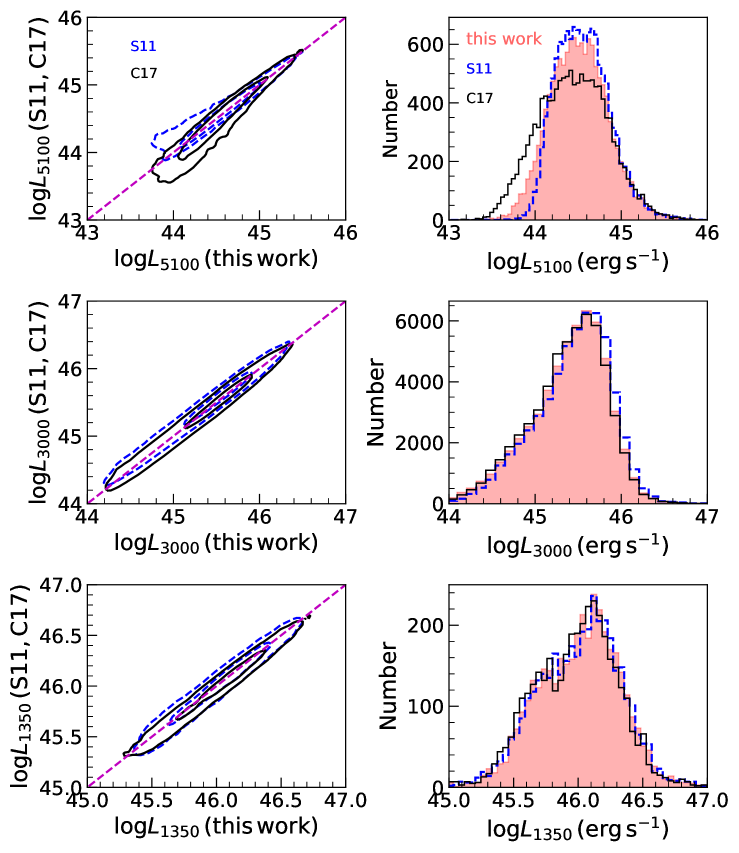
Figure 6: Comparison of continuum luminosity measurements between our work and S11 and C17 for all the common quasars. The inner and outer contours are the $1\sigma$ and $2\sigma$ density contours. The one-to-one line is also shown.

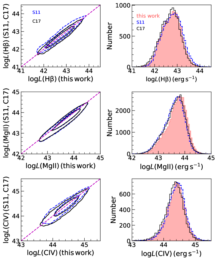
Figure 7: Same as in Figure 6 but for line luminosities.

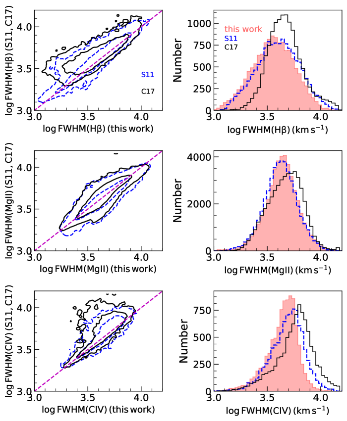
Figure 8: Same as in Figure 6 but for line FWHM.

3 Comparison with previous studies

We compared our measurements with S11 and C17 catalogs. The former catalog is based on all DR7 quasars up to $z=5$ with 105,783 entries while the later is based on DR10 quasars up to $z=2$ with 71,261 entries (catalog version “qsfit$\_$1.2.4”). Although different methods were used by both the authors than the PyQSOFit code used in our analysis, a comparison can be made. We refer the readers to Calderone et al. (2017) for a discussion on S11 and C17 spectral analysis methods. Here we summarize the main differences

1. S11 didn’t decompose host galaxy contamination. C17 used an elliptical galaxy template to represent the host galaxy contamination. We subtracted host galaxy contribution using the PCA method with 5 PCA components for galaxy (see section 2.1).

2. S11 modeled local AGN continuum (using a power-law) including Fe II emission then fitted the emission lines of the continuum and Fe II subtracted spectrum. C17 fitted continuum (power-law + Balmer continuum) of the whole spectrum and at the final fitting step, they fitted all components (continuum + galaxy + iron + emission lines) simultaneously. We first removed the host galaxy contribution if present and then fitted AGN continuum (power-law + Balmer continuum) and Fe II template of the whole host subtracted spectrum. Finally, we fitted the emission lines of the continuum subtracted spectrum.

3. Both S11 and C17 used the UV Fe II template from Vestergaard & Wilkes (2001), which is limited to $3090\AA$, while the UV Fe II template used in this work has an extended coverage up to $3500\AA$.

4. S11 fitted broad lines with up to three Gaussian while C17 started their modeling of broad lines with single Gaussian (‘known’ line) and added more Gaussian if ‘unknown’ emission lines are present close to the known lines. We fitted most of the broad emission lines using multiple Gaussians (see Table 1).

We cross-matched our catalog with S11 and C17 using TOPCAT (Taylor, 2005) and took only the common entries (71,163) for comparison. However, different catalogs may include spectra of different quality for the same target as repeated observations have been performed by SDSS. Quasars also show spectral variability, which can affect the measurements included in different catalogs. Therefore, we cross-matched sources having the same SDSS plate-mjd-fiber in all three catalogs and found 65,170 matches. Furthermore, we only included measurements having a quality flag of 0 in both C17 and our work.

In Figure 6, we compare our continuum luminosity measurements with S11 and C17 where our measurements are plotted along the x-axis in the left panels. We also plot the distribution of measurements for all three catalogs in the right panels. In general, we find excellent agreement between the measurements. The mean and standard deviation of the difference between this work and S11 (C17) is $0.001\pm 0.052$ ($0.023\pm 0.031$) dex for $L_{1350}$ (3827 sources), $-0.054\pm 0.055$ ($0.010\pm 0.052$) dex for $L_{3000}$ (56,577 sources) and $-0.045\pm 0.104$ ($0.067\pm 0.122$) dex for $L_{5100}$ (12,967 sources). We notice a larger difference in the estimates of $L_{5100}$ compared to other luminosities between S11, C17 and our work but mainly for low-luminosity quasars. Our estimates of $L_{5100}$ lie in between S11 and C17. We attribute this difference due to differences in the host galaxy subtraction procedures. For example, S11 did not perform host galaxy decomposition, thus, their measurements are contaminated by the host galaxy contribution. On the other hand, C17 used a single 5 Gyr old elliptical galaxy template to subtract the host galaxy contribution, while, we used the PCA method implemented in PyQSOFit to subtract the host galaxy (see section 2.1). Although the PCA host decomposition method allowed us to systematically decompose stellar contribution from a large number of spectra, it is a simplistic approach and in principle one can use other host galaxy decomposition methods (e.g., Matsuoka et al., 2015; Rakshit & Woo, 2018) using different stellar templates (e.g., Bruzual & Charlot, 2003; Valdes et al., 2004) to decompose the stellar contribution from the spectra of quasars.

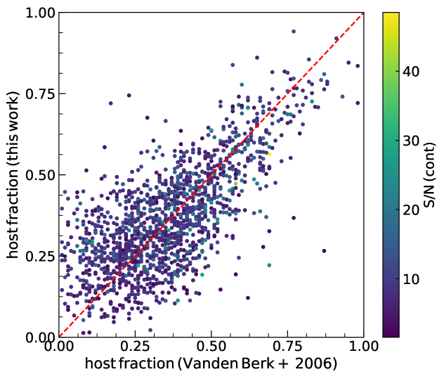
Figure 9: Host galaxy fraction to that of the total flux in the wavelength range of 4160-4210Å  in this work (y-axis) is compared to that of Vanden Berk et al. (2006) color codded by continuum S/N. The one-to-one line is also plotted (dashed-line).

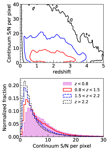
Figure 10: Top: The median continuum S/N per pixel is plotted against redshift. The 1$\sigma$ (red), 2$\sigma$ (blue) and 3$\sigma$ (black) density contours are shown. Bottom: Normalized distribution (i.e. the area under each histogram is unity) of continuum S/N for different redshift range. The x-axis is limited to 30.

In Figure 7, we compare the H$\beta$ (top), Mg ii (middle) and C iv (bottom) line luminosity measurements between all three catalogs. In all cases, we found strong agreement. The mean and standard deviation of H$\beta$ (13,177 sources) line luminosity between this work and S11 (C17) are $-0.045\pm 0.111$ ($0.044\pm 0.109$) dex, while the same for Mg ii (45,048 sources) and C iv (9,384 sources) line luminosities are $0.094\pm 0.083$ ($0.067\pm 0.088$) dex and $-0.014\pm 0.106$ ($0.043\pm 0.106$) dex, respectively. All the line luminosity plots show a strong correlation with the Spearman rank correlation coefficient $r_{s}>0.95$ for both H$\beta$ and Mg ii lines, while 0.94 (0.93) for C iv line luminosity between this work and SII (C17). We note that compared to H$\beta$ and CIV line luminosities, Mg II line luminosity shows a larger offset. Our estimated Mg II luminosity is slightly larger compared to S11 and C17. This could be due to the use of different UV Fe II templates. For example, Shin et al. (2019) found that Tsuzuki et al. (2006) template provides an average 0.13 dex higher Mg II flux and 0.10 dex lower UV Fe II flux compared to Vestergaard & Wilkes (2001) template.

The emission line widths in different catalogs are less strongly correlated (Figure 8) having $r_{s}=0.85$ (0.75) for H$\beta$, 0.82 (0.82) for Mg ii and 0.72 (0.45) for C iv between this work and S11 (C17) indicating the complexity in the measurement of FWHM. The mean and standard deviation between this work and S11 (C17) is $-0.045\pm 0.113$ ($-0.111\pm 0.140$) dex for H$\beta$, $0.011\pm 0.097$ ($-0.031\pm 0.100$) dex for Mg ii and $-0.048\pm 0.119$ ($-0.118\pm 0.173$) dex for C iv line width measurement. We note that on average our FWHM measurements are more consistent with S11 compared to C17. Although a slight discrepancy between different catalogs is found, measurements are in general agreement with S11 and C17. The discrepancy between different catalogs is due to the use of different spectral decomposition methods as mentioned above.

We compared our estimated host fraction with that of Vanden Berk et al. (2006) where the host fraction, the ratio of host flux to the total flux, is estimated in the wavelength range of 4160-4210Å. To avoid any difference due to the spectral quality between the two catalogs, we only considered objects having the same spectra in both the works (SDSS plate-mjd-fiber). There are 1486 sources, which have host contribution $>0$ in both the works. We plotted them in Figure 9 (color-codded by continuum S/N). Our results are consistent with them having a median ratio (our to their) of $1.01^{+0.58}_{-0.31}$. Therefore, our stellar fraction measurements are consistent with that of Vanden Berk et al. (2006).

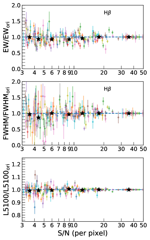
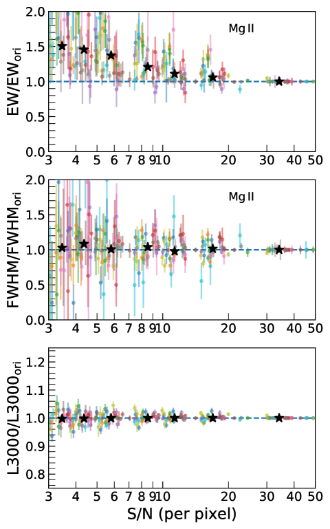
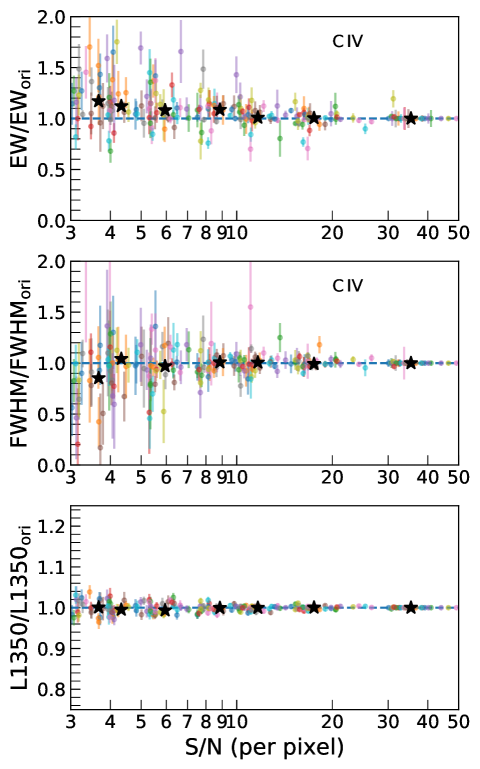
Figure 11: The ratio of EW (top), FWHM (middle) and continuum luminosity (bottom) of the S/N degraded spectra to the original spectra. A sample of 30 high-S/N spectra (measurement from individual spectrum is represented by an unique color) was chosen for each line and their S/N is degraded by adding noise by a factor of 2, 3, 4, 6, 8 and 10 to their original flux errors. The sample median is also shown (star-marker). Although on average the measurements are consistent up to a very low S/N $\sim 3$, any individual spectrum can deviate by 50% or more.

4 Impact of S/N on spectral quantities

Although spectral decomposition of high S/N spectra can be reliable, the decomposition of low S/N spectra is usually difficult. In Figure 10, we plot the density contours of median continuum S/N with redshift in the upper panel and the distribution of median continuum S/N at different redshift range in the lower panel. The tail of the S/N distribution decreases rapidly at higher redshift. At low redshift $z<0.8$, the fraction of sources with S/N$>3$ pixel^-1 is 84%, while for high-redshift $z>2.2$, the fraction of sources with S/N$>3$ pixel^-1 is 54%. The total number of sources with S/N$>3$ pixel^-1 in our catalog is 332,204 i.e., about 63% of the total sample.

Several authors (e.g., Shen et al., 2011; Denney et al., 2016; Shen et al., 2019) have investigated the impact of S/N on the spectral decomposition method. They found that for high equivalent width (EW) objects, FWHMs and EWs are biased by less than $\pm 20$% if line S/N reduced to as low as about 3, while for low-EW objects, the FWHMs and EWs are biased by $>20$% for $S/N<5$. However, in all cases even at very low S/N, continuum luminosity measurements are unbiased. To investigate the impact of S/N on the measurement of our spectral quantities, we followed an approach similar to the previous studies. First, we selected a sample of thirty high-S/N original spectra independently for H$\beta$ in the redshift of $z<0.8$, Mg II in the redshift range of $z=0.8-1.8$ and CIV in the redshift range of $z=1.8-3.2$. Then for each spectrum, we multiplied a constant factor of 2, 3, 4, 6, 8 and 10 to their original flux errors and added to the original spectrum a Gaussian random deviate of zero mean and standard deviation given by the new flux errors. We then repeated our spectral decomposition method as used in the decomposition of high-S/N original spectra, re-measured all the spectral quantities from the de-graded spectra, and finally compared them with the high-S/N original spectra. In Figure 11, we plot the ratio of the measurements from degraded spectra to the original high-S/N spectra as a function of the median continuum S/N for all thirty objects for each line (measurement from individual spectrum is represented by an unique color). With decreasing S/N, measurement uncertainties increase as per expectation. For example, when the sample median S/N reduced by a factor of 10 from 36.5 to 3.6, uncertainty in EW increased from 4.8Å  to 10.2Å, and uncertainty in FWHM increased from 221 km s^-1 to 1246 km s^-1. The offsets represented by the sample median (star-marker) are negligible even at very low S/N suggesting the measurements are unbiased. However, measurements of any individual spectrum can have 50% or more deviation. The Mg II EW (top-middle) shows a systematic offsets with decreasing S/N. However, this is not present in the case of H$\beta$ (top-left) and CIV (top-right) EW. The reason of this offset in Mg II could be due to the blending UV Fe II and Mg II line. The continuum luminosity is unbiased even at very low S/N.

The above investigation suggests that on average our spectral decomposition method recovers the measurements of the high S/N ratio spectra although individual measurements can deviate by 50% or more. For peculiar sources, e.g., ones with double peak emission line our decomposition may fail badly. For this purpose, we provide various quality flags for each object, as described in detail in Appendix A, based on several criteria. These quality flags give the reliability of our measurements.

Figure 12: The H$\alpha$ (top), H$\beta$ (middle) and [O III] ($\lambda$5007) line luminosities is plotted against 5100Å continuum luminosity. The best linear fit using linmix is shown by the black-dashed line while the fits obtained by bces considering x-axis as independent variable (blue dashed-dot line), y-axis as independent variable (cyan dotted line) and orthogonal least squares fit (magenta-dashed line) are shown. The 20 (white), 40 (cyan), 68 (blue) and 95 (green) percentile density contours along with the density map are shown.

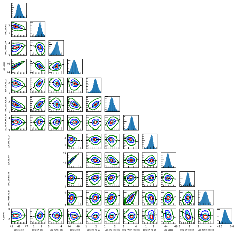
Figure 13: Correlation between various quasar parameters for objects with quality flag $=0$. Linear fits to the diagram is shown by a straight line in each plot using linmix. The corresponding best fit coefficients are mentioned in Table 2. The 20 (red), 40 (cyan), 68 (blue) and 95 (green) percentile density contours are also shown. The histograms are the projected one-dimensional distributions.

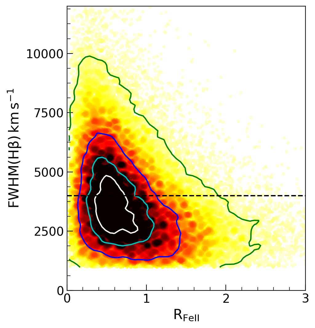
Figure 14: H$\beta$ line width vs. optical Fe ii strength. The 20, 40, 68 and 95 percentile density contours along with the density map are shown. The horizontal line at 4000 km s^-1 is also shown.

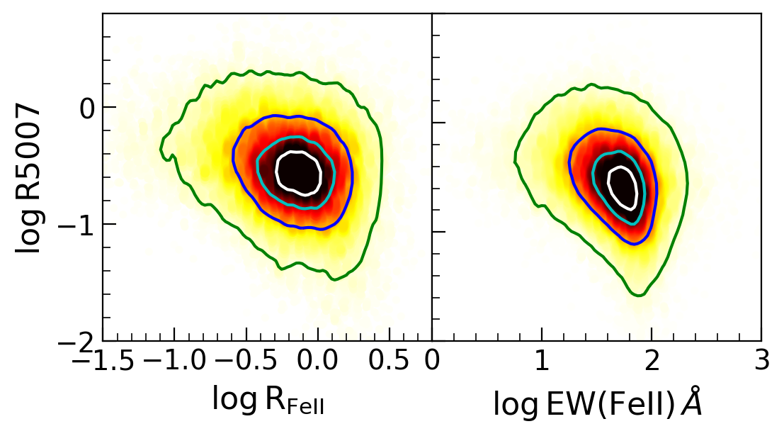
Figure 15: The R5007 (ratio of [O iii] to H$\beta$ equivalent width) against R${}_{\mathrm{Fe\,\textsc{ii}}}$ (left) and Fe ii equivalent width (right). The 20, 40, 68 and 95 percentile density contours along with the density map are shown.

5 Applications

5.1 Correlation analysis

The spectral catalog generated in this work for a large number of quasars can be used to investigate the correlation between various line and continuum properties in detail. Here, we studied some of the correlations. For this, we considered measurements with a quality flag of zero. The luminosity of Balmer lines show strong correlation with the monochromatic continuum luminosity at 5100 Å over a wide range of redshift and luminosity suggesting that the physical mechanisms behind the correlation are the same in different AGN across all redshift and luminosity range (e.g., Greene & Ho, 2005; Jun et al., 2015; Rakshit et al., 2017). In Figure 12, we plot the luminosity of H$\alpha$ (top panel) and H$\beta$ (middle panel) against $L_{5100}$. In both cases, a strong correlation is found with $r_{s}$ of 0.93 and 0.86, respectively. We performed linear regression analysis with measurement errors on both axes using Bayesian code linmix (Kelly, 2007) and obtained

$$\log L(H\alpha)=(1.126\pm 0.004)\log L(5100)+(-6.89\pm 0.20)$$ (5)

$$\log L(H\beta)=(0.947\pm 0.002)\log L(5100)+(-0.45\pm 0.09)$$ (6)

with an intrinsic scatter of $0.025\pm 0.001$ and $0.035\pm 0.001$, respectively. These correlations are shown by the black dashed line in Figure 12. For equation 5, a linear regression using bces (Akritas & Bershady, 1996; Nemmen et al., 2012) gives a slope (m) of $1.125\pm 0.005$ and intercept (c) of $-6.86\pm 0.22$ considering $\log L(5100)$ as the independent variable (blue dashed-dot line), m$=1.264\pm 0.006$ and c$=-12.97\pm 0.27$ considering $\log L(H\alpha)$ as the independent variable (cyan dotted line) and m$=1.120\pm 0.005$ and c$=-10.37\pm 0.25$ for orthogonal least squares (magenta-dashed line). The same for equation 6 is found to be $0.937\pm 0.002$ and $0.89\pm 0.11$ (m, c) for $\log L(5100)$ as independent variable, m$=1.177\pm 0.002$ and c$=-9.75\pm 0.11$ considering $\log L(H\beta)$ as the independent variable and m$=1.057\pm 0.002$ and c$=-4.41\pm 0.10$ for orthogonal least squares. The slopes of the $\log L(H\alpha)-\log L(5100)$ and $\log L(H\beta)-\log L(5100)$ correlations agree with the previous studies. For example, using a sample of low-z ($z<0.35$) SDSS quasars, Greene & Ho (2005) found a slope of $1.157\pm 0.005$ for equation 5 and $1.133\pm 0.005$ for equation 6. For high redshift ($z=1.5-2.2$) and high-luminosity ($\log L_{5100}=45.4-47.0$) quasars, Shen & Liu (2012) obtained a slope of $1.010\pm 0.042$ and $1.251\pm 0.067$ for equations 5 and 6, respectively. Jun et al. (2015) investigated $\log L(H\alpha)-\log L(5100)$ correlation using quasars of $z=0.0-6.2$ and luminosity of $\log L_{5100}=41.7-47.2$ and obtained a slope of $1.044\pm 0.008$.

The correlation between $L\mathrm{[OIII]}-L(5100)$ has been widely used to estimate bolometric luminosity for Type 2 AGN since their host galaxy contamination prevents reliable estimation of $L_{5100}$ (see Kauffmann et al., 2003; Heckman et al., 2004). However, this relation has a large scatter (Heckman et al., 2004; Shen et al., 2011). The L([O III]$\lambda 5007$) as a function of $L_{5100}$ is plotted in the bottom panel ($r_{s}=0.58$) of Figure 12. The best-fit linear regression using linmix gives

$$\log L\mathrm{[OIII]}=(0.720\pm 0.003)\log L(5100)+(10.08\pm 0.13)$$ (7)

with an intrinsic scatter of $0.102\pm 0.001$. But the same using bces is found to be m$=0.693\pm 0.003$ and c$=11.24\pm 0.15$ when $\log L(5100)$ is the independent variable, m$=1.347\pm 0.031$ and c$=-17.74\pm 1.41$ when $\log L\mathrm{[OIII]}$ is the independent variable and m$=0.953\pm 0.015$ and c$=-0.30\pm 0.69$ for orthogonal least squares. Depending on the treatment of the independent variable, the $L\mathrm{[OIII]}-L(5100)$ relation shows a range of slopes of $0.7$ to $1.3$ due to large scatter. This agrees with Shen et al. (2011), who noted a scatter of $\sim$0.4 dex around the best-fit $L\mathrm{[OIII]}-L(5100)$ relation and a slope of 0.77 when $L_{5100}$ is considered as the independent variable, and 1.34 for bisector linear regression fit.

In Figure 13, we plot various such line and continuum quantities and performed correlation analysis between them. The fits to the data are shown by dashed lines in Figure 13 and the results of the fitting are given in Table 2. Most of the correlation agrees with the previous works based on smaller samples. For example, the continuum luminosity at 1350Å, 3000Å, and 5100Å  are strongly correlated with each other (e.g., Jun et al., 2015). The line width of H$\beta$ and Mg II shows a strong correlation (e.g., Wang et al., 2009), however, the correlation is very weak between Mg II and CIV line FWHM. All the parameters are uncorrelated with spectral index except for a weak anti-correlation with $L_{5100}$ and H$\beta$ EW (Shen et al., 2011). Emission line FWHM is weakly correlated with line EW both for H$\beta$ and Mg II lines similar to what has been noted for Mg II line by Dong et al. (2009). The well-known anti-correlation between continuum luminosity and line EW is found both for Mg II and CIV (Baldwin, 1977) but not for H$\beta$ EW. Although no correlation between EW of optical Fe II (measured from the best-fit optical Fe II template in the wavelength range of 4435-4685$\AA$) and EW of H$\beta$ is found, EW of UV Fe II (measured from the best-fit UV Fe II template in the wavelength range of 2200-3090$\AA$) is strongly correlated with the EW of Mg II line and C IV (e.g., Kovačević-Dojčinović & Popović, 2015).

Table 2: Linear regression analysis to the y vs. x correlation for objects with quality flag =0 using linmix having slope (m), intercept (c) and intrinsic scatter ($\sigma_{\mathrm{int}}$). The Spearman rank correlation coefficient ($r_{s}$) is also noted.

y	x	m	c	$\sigma_{\mathrm{int}}$	$r_{s}$
PL_SLOPE	LOG_FWHM_HB_BR	$-$0.280 $\pm$ 0.018	$-$0.239 $\pm$ 0.064	0.463 $\pm$ 0.003	$-$0.09
PL_SLOPE	LOG_EW_HB_BR	$-$1.051 $\pm$ 0.017	0.702 $\pm$ 0.030	0.445 $\pm$ 0.003	$-$0.30
PL_SLOPE	LOG_L5100	$-$0.389 $\pm$ 0.006	16.100 $\pm$ 0.256	0.508 $\pm$ 0.003	$-$0.24
PL_SLOPE	LOG_EW_FE_OP	0.040 $\pm$ 0.013	$-$1.308 $\pm$ 0.021	0.492 $\pm$ 0.003	$-$0.05
PL_SLOPE	LOG_FWHM_MGII_BR	0.317 $\pm$ 0.008	$-$2.476 $\pm$ 0.030	0.311 $\pm$ 0.001	0.03
PL_SLOPE	LOG_EW_MGII_BR	0.420 $\pm$ 0.005	$-$2.042 $\pm$ 0.009	0.313 $\pm$ 0.001	0.15
PL_SLOPE	LOG_EW_FE_UV	0.250 $\pm$ 0.005	$-$1.816 $\pm$ 0.010	0.297 $\pm$ 0.001	0.07
PL_SLOPE	LOG_L3000	$-$0.183 $\pm$ 0.002	6.972 $\pm$ 0.073	0.341 $\pm$ 0.001	$-$0.12
PL_SLOPE	LOG_FWHM_CIV	$-$0.293 $\pm$ 0.007	$-$0.208 $\pm$ 0.024	0.258 $\pm$ 0.001	$-$0.08
PL_SLOPE	LOG_EW_CIV	0.274 $\pm$ 0.004	$-$1.754 $\pm$ 0.008	0.254 $\pm$ 0.001	0.15
PL_SLOPE	LOG_L1350	$-$0.057 $\pm$ 0.002	1.407 $\pm$ 0.100	0.317 $\pm$ 0.001	$-$0.03
LOG_FWHM_HB_BR	LOG_EW_HB_BR	0.260 $\pm$ 0.005	3.087 $\pm$ 0.008	0.031 $\pm$ 0.001	0.22
LOG_FWHM_HB_BR	LOG_L5100	0.072 $\pm$ 0.002	0.338 $\pm$ 0.086	0.030 $\pm$ 0.001	0.16
LOG_FWHM_HB_BR	LOG_EW_FE_OP	$-$0.159 $\pm$ 0.004	3.829 $\pm$ 0.006	0.030 $\pm$ 0.001	$-$0.21
LOG_FWHM_HB_BR	LOG_FWHM_MGII_BR	1.023 $\pm$ 0.004	$-$0.089 $\pm$ 0.014	0.005 $\pm$ 0.001	0.67
LOG_FWHM_HB_BR	LOG_EW_MGII_BR	0.243 $\pm$ 0.004	3.171 $\pm$ 0.007	0.024 $\pm$ 0.001	0.21
LOG_FWHM_HB_BR	LOG_EW_FE_UV	0.082 $\pm$ 0.005	3.420 $\pm$ 0.010	0.024 $\pm$ 0.001	0.09
LOG_FWHM_HB_BR	LOG_L3000	0.064 $\pm$ 0.002	0.730 $\pm$ 0.075	0.030 $\pm$ 0.001	0.17
LOG_EW_HB_BR	LOG_L5100	$-$0.049 $\pm$ 0.002	3.987 $\pm$ 0.091	0.034 $\pm$ 0.001	$-$0.04
LOG_EW_HB_BR	LOG_EW_FE_OP	0.209 $\pm$ 0.003	1.491 $\pm$ 0.005	0.027 $\pm$ 0.001	0.24
LOG_EW_HB_BR	LOG_FWHM_MGII_BR	0.112 $\pm$ 0.007	1.433 $\pm$ 0.027	0.037 $\pm$ 0.001	0.09
LOG_EW_HB_BR	LOG_EW_MGII_BR	0.288 $\pm$ 0.005	1.354 $\pm$ 0.008	0.035 $\pm$ 0.001	0.24
LOG_EW_HB_BR	LOG_EW_FE_UV	0.240 $\pm$ 0.006	1.367 $\pm$ 0.012	0.041 $\pm$ 0.001	0.21
LOG_EW_HB_BR	LOG_L3000	$-$0.005 $\pm$ 0.002	2.029 $\pm$ 0.083	0.034 $\pm$ 0.001	0.04
LOG_L5100	LOG_EW_FE_OP	$-$0.022 $\pm$ 0.006	44.438 $\pm$ 0.011	0.150 $\pm$ 0.001	0.02
LOG_L5100	LOG_FWHM_MGII_BR	0.169 $\pm$ 0.009	43.874 $\pm$ 0.034	0.135 $\pm$ 0.001	0.10
LOG_L5100	LOG_EW_MGII_BR	$-$0.752 $\pm$ 0.006	45.792 $\pm$ 0.010	0.107 $\pm$ 0.001	$-$0.42
LOG_L5100	LOG_EW_FE_UV	$-$0.463 $\pm$ 0.007	45.396 $\pm$ 0.014	0.118 $\pm$ 0.001	$-$0.24
LOG_L5100	LOG_L3000	0.806 $\pm$ 0.001	8.576 $\pm$ 0.044	0.019 $\pm$ 0.001	0.93
LOG_EW_FE_OP	LOG_FWHM_MGII_BR	$-$0.450 $\pm$ 0.009	3.312 $\pm$ 0.033	0.053 $\pm$ 0.001	$-$0.24
LOG_EW_FE_OP	LOG_EW_MGII_BR	$-$0.068 $\pm$ 0.007	1.820 $\pm$ 0.012	0.057 $\pm$ 0.001	$-$0.13
LOG_EW_FE_OP	LOG_EW_FE_UV	0.094 $\pm$ 0.008	1.564 $\pm$ 0.015	0.047 $\pm$ 0.001	0.00
LOG_EW_FE_OP	LOG_L3000	$-$0.025 $\pm$ 0.003	2.792 $\pm$ 0.119	0.062 $\pm$ 0.001	0.00
LOG_FWHM_MGII_BR	LOG_EW_MGII_BR	0.262 $\pm$ 0.001	3.207 $\pm$ 0.002	0.017 $\pm$ 0.001	0.32
LOG_FWHM_MGII_BR	LOG_EW_FE_UV	0.103 $\pm$ 0.001	3.461 $\pm$ 0.003	0.018 $\pm$ 0.001	0.12
LOG_FWHM_MGII_BR	LOG_L3000	0.014 $\pm$ 0.001	3.041 $\pm$ 0.025	0.019 $\pm$ 0.001	0.06
LOG_FWHM_MGII_BR	LOG_FWHM_CIV	0.241 $\pm$ 0.003	2.797 $\pm$ 0.013	0.013 $\pm$ 0.001	0.17
LOG_FWHM_MGII_BR	LOG_EW_CIV	0.064 $\pm$ 0.002	3.563 $\pm$ 0.003	0.014 $\pm$ 0.001	0.06
LOG_FWHM_MGII_BR	LOG_L1350	$-$0.031 $\pm$ 0.001	5.100 $\pm$ 0.045	0.015 $\pm$ 0.001	$-$0.02
LOG_EW_MGII_BR	LOG_EW_FE_UV	0.708 $\pm$ 0.002	0.342 $\pm$ 0.003	0.021 $\pm$ 0.001	0.58
LOG_EW_MGII_BR	LOG_L3000	$-$0.214 $\pm$ 0.001	11.388 $\pm$ 0.029	0.033 $\pm$ 0.001	$-$0.49
LOG_EW_MGII_BR	LOG_FWHM_CIV	$-$0.215 $\pm$ 0.006	2.511 $\pm$ 0.020	0.047 $\pm$ 0.001	$-$0.12
LOG_EW_MGII_BR	LOG_EW_CIV	0.536 $\pm$ 0.002	0.781 $\pm$ 0.004	0.026 $\pm$ 0.001	0.62
LOG_EW_MGII_BR	LOG_L1350	$-$0.338 $\pm$ 0.001	17.098 $\pm$ 0.064	0.028 $\pm$ 0.001	$-$0.65
LOG_EW_FE_UV	LOG_L3000	$-$0.146 $\pm$ 0.001	8.516 $\pm$ 0.039	0.043 $\pm$ 0.001	$-$0.27
LOG_EW_FE_UV	LOG_FWHM_CIV	$-$0.257 $\pm$ 0.006	2.882 $\pm$ 0.022	0.047 $\pm$ 0.001	$-$0.10
LOG_EW_FE_UV	LOG_EW_CIV	0.515 $\pm$ 0.003	1.048 $\pm$ 0.005	0.029 $\pm$ 0.001	0.54
LOG_EW_FE_UV	LOG_L1350	$-$0.217 $\pm$ 0.002	11.805 $\pm$ 0.084	0.043 $\pm$ 0.001	$-$0.31
LOG_L3000	LOG_FWHM_CIV	0.784 $\pm$ 0.007	42.513 $\pm$ 0.027	0.173 $\pm$ 0.001	0.28
LOG_L3000	LOG_EW_CIV	$-$0.952 $\pm$ 0.003	47.099 $\pm$ 0.006	0.120 $\pm$ 0.001	$-$0.57
LOG_L3000	LOG_L1350	0.896 $\pm$ 0.001	4.624 $\pm$ 0.047	0.033 $\pm$ 0.001	0.91
LOG_FWHM_CIV	LOG_EW_CIV	$-$0.179 $\pm$ 0.002	3.938 $\pm$ 0.003	0.025 $\pm$ 0.001	$-$0.21
LOG_FWHM_CIV	LOG_L1350	0.129 $\pm$ 0.001	$-$2.278 $\pm$ 0.038	0.024 $\pm$ 0.001	0.33
LOG_EW_CIV	LOG_L1350	$-$0.305 $\pm$ 0.001	15.749 $\pm$ 0.042	0.038 $\pm$ 0.001	$-$0.53

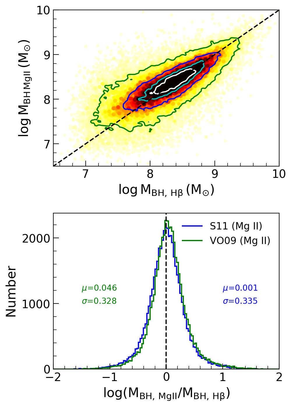
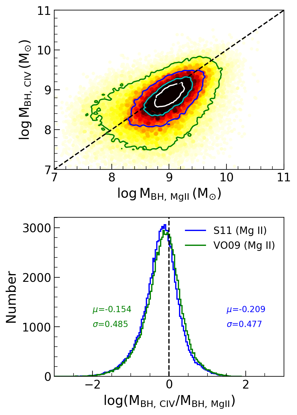
Figure 16: Left: Comparison between black holes masses estimated based on Mg ii and H$\beta$ line. The distribution of the mass ratios is shown in the lower panel along with the number of objects for which both the masses were estimated, sample mean ($\mu$) and dispersion ($\sigma$) are noted. Right: Comparison between C iv and Mg ii based mass measurements for objects having both the lines. The offset and dispersion of M${}_{\mathrm{BH,C\textsc{iv}}}$/M_BH,MgII is larger than that of M_BH,MgII/M_BH,Hβ. The 20, 40, 68 and 95 percentile density contours along with the density map are shown in the upper panels. Only sources with quality flag =0 are included.

Boroson & Green (1992) performed PCA using a sample of 87 PG quasars ($z<0.5$) and found various correlations involving optical Fe II, [O III]5007 and H$\beta$ broad component, radio to optical flux ratio and the optical to X-ray spectral index. The first PCA eigenvector (Eigenvector 1; hereafter E1) strongly anti-correlates with $R_{\mathrm{Fe\,II}}$ (defined by the ratio of the EW of Fe II (4435$-$4685Å ) to H$\beta$ broad line) and luminosity of [O III]$\lambda 4959,5007$. The main parameters of the well-known 4DE1 (Sulentic et al., 2000b, 2002), which can account for the diverse nature of broad line AGN, are the FWHM of broad H$\beta$ line and $R_{\mathrm{Fe\,\textsc{ii}}}$. These two quantities are plotted in Figure 14 for objects with quality flag =0 in the catalog. Firstly, quasars with a wide range of Fe ii strength can be found at a given FWHM(H$\beta$). Similarly, at a given Fe ii strength, the H$\beta$ can have a large range. The $R_{\mathrm{Fe\,II}}$ distribution peaks at $\sim 0.7$ which can be occupied by quasars with FWHM(H$\beta$) of $\sim 1000-10,000$ km s^-1. This dispersion is suggested to be due to an orientation effect (see Shen & Ho, 2014; Sun & Shen, 2015). Secondly, the well-known trend of decreasing FWHM with increasing $R_{\mathrm{FeII}}$ is noticed as also shown in previous studies (e.g., Shen et al., 2011; Coffey et al., 2019). Thus, quasars with a very broad H$\beta$ line and strong Fe ii strength is rare, especially in the low redshift SDSS sample. However, IR spectroscopic study of high-z quasars shows a systematically larger FWHM(H$\beta$) compared to the low-z sources at high $R_{\mathrm{Fe\,II}}$ (Shen, 2016). The dashed line represents the separation of quasars into two populations; the population A (FWHM(H$\beta$, broad) $\leq 4000$ km s^-1) sources with strong Fe ii and soft X-ray excess, and population B (FWHM(H$\beta$, broad) $>4000$ km s^-1) sources with weak Fe ii and a lack of soft X-ray excess (Sulentic et al., 2000a).

Previous studies found an anti-correlation between [O iii] and Fe ii emission, i.e., objects with strong [O iii] are found to be weak Fe ii emitters and vice versa (e.g., Boroson & Green, 1992; Grupe et al., 1999; McIntosh et al., 1999; Rakshit et al., 2017) although Véron-Cetty et al. (2001) found such anti-correlation to be very weak. In Figure 15, we plot R5007, i.e. the ratio of EW of [O III]5007 to the EW of total H$\beta$ (sum of the EW of broad and narrow H$\beta$ components) against R${}_{\mathrm{Fe\,\textsc{ii}}}$ (left) and EW of Fe ii (right). We found that the anti-correlation, although weak, is present with correlation coefficient $r_{s}=-0.23$ between R5007 and R${}_{\mathrm{Fe\,\textsc{ii}}}$, while the R5007 vs. EW (Fe ii) anti-correlation is moderately strong with $r_{s}=-0.32$. The anti-correlations become stronger with $r_{s}=-0.37$ for R5007 vs. R${}_{\mathrm{Fe\,II}}$ and $r_{s}=-0.45$ for R5007 vs. EW (Fe II) when sources with continuum S/N$>10$ pixel^-1 is considered. The correlation found here is consistent with previous studies. For example, Boroson & Green (1992) found $r_{s}=-0.36$ for R5007 vs. R${}_{\mathrm{Fe\,II}}$ relation and $-0.52$ for R5007 vs. EW (Fe II) relation. Similarly, McIntosh et al. (1999) found $r_{s}=-0.43$ for R5007 vs. R${}_{\mathrm{Fe\,II}}$ relation and $r_{s}=-0.54$ for R5007 vs. EW (Fe II) relation while Grupe et al. (1999) found $r_{s}=-0.36$ for R5007 vs. EW (Fe II) relation. Therefore, the strong Fe ii sources may have weak [O iii] emission or vice versa.

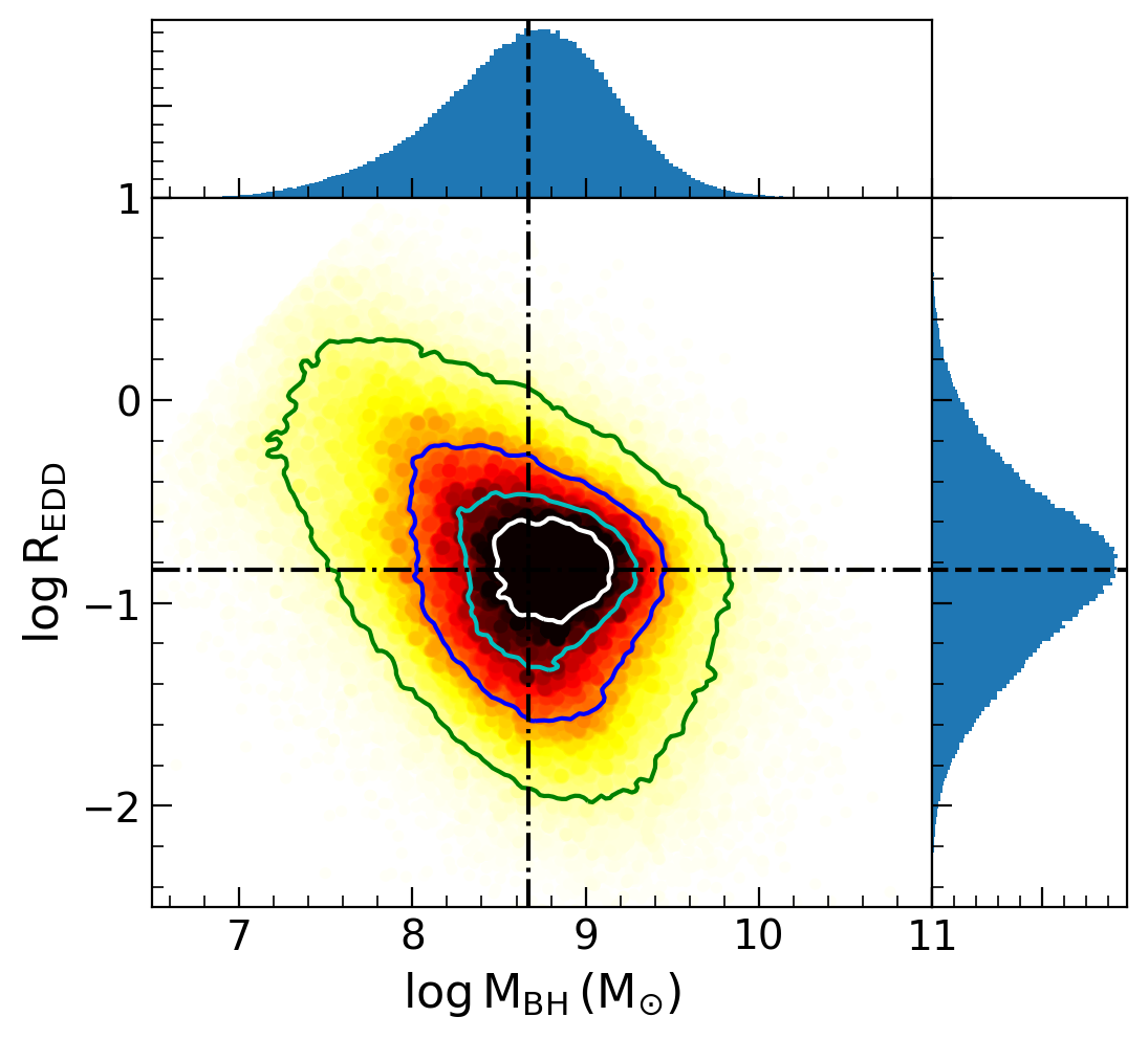
Figure 17: Eddington ratio vs. black hole masses for all quasars in the catalog. The dashed lines represent the median of the distribution. The 20, 40, 68 and 95 percentile density contours along with the density map are shown. Only sources with quality flag =0 are included.

5.2 Black hole mass measurement

The value of $M_{\mathrm{BH}}$ in an AGN can be estimated using virial relation from single-epoch spectrum for which continuum luminosity and line width measurements are available as follows

$$\log\left(\frac{M_{\mathrm{BH}}}{M_{\odot}}\right)=A+B\log\left(\frac{\lambda L_{\lambda}}{10^{44}\mathrm{erg\,s^{-1}}}\right)+2\log\left(\frac{\mathrm{FWHM}}{\mathrm{km\,s^{-1}}}\right)$$ (8)

where $A$ and $B$ are the constants empirically calibrated by various authors using reverberation mapping $R-L$ relations of local AGN (Kaspi et al., 2000, 2005; Bentz et al., 2013) as well as internally calibrated based on the availability of multiple strong emission lines such as Mg ii with H$\beta$ (e.g., McLure & Jarvis, 2002; McLure & Dunlop, 2004; Vestergaard & Peterson, 2006; Shen et al., 2011; Woo et al., 2018) and C iv with Mg ii or H$\beta$ (e.g., Vestergaard & Peterson, 2006; Assef et al., 2011; Park et al., 2017). In this work, we used the black hole mass calibrations from Vestergaard & Peterson (2006, thereafter VP06), Assef et al. (2011, thereafter A11), Vestergaard & Osmer (2009, thereafter VO09) and S11.

$$A,B=\begin{cases}(0.910,0.50),&\text{for H$\beta$; VP06}\\ (0.895,0.52),&\text{for H$\beta$; A11}\\ (0.860,0.50),&\text{for Mg {ii}; VO09}\\ (0.740,0.62),&\text{for Mg {ii}; S11}\\ (0.660,0.53),&\text{for C {iv}; VP06}\end{cases}$$

We caution that the derived virial $M_{\mathrm{BH}}$ values could have uncertainty $>0.4$ dex due to the different systematics (e.g., different line width measures, geometry and kinematics of BLR, see Collin et al., 2006; Shen, 2013) involved in the calibrations used, which have not been taken in to account. The uncertainties in the virial $M_{\mathrm{BH}}$ values that are provided in the catalog are only the measurement uncertainties calculated via error propagation of Equation 8. In Figure 16 we compare $M_{\mathrm{BH}}$ calculated using different lines. We plot Mg II based black hole masses against H$\beta$ (upper left) and the ratio of the two masses (lower panels). Both S11 and VO09 provide consistent Mg II based masses with negligible offsets between Mg II and H$\beta$ based masses but with a dispersion of $\sim 0.3$. In the right panel, we compare CIV based masses against Mg II based masses. Here, we notice a larger offset and dispersion in the ratio of CIV to Mg II based masses compared to Mg II to H$\beta$ based mass ratio. In the catalog, we provide ‘fiducial’ virial $M_{\mathrm{BH}}$ values calculated based on (a) H$\beta$ line (for $z<0.8$) using the calibration of VP06, (b) Mg ii line (for $0.8\leq z<1.9$) using the calibration provided by VO09, and (c) C iv line (for $z\geq 1.9$) using VP06 calibration.

We estimated Eddington ratio ($R_{\mathrm{Edd}}$), which is the ratio of bolometric (see section 2.3) to Eddington luminosity ($L_{\mathrm{Edd}}$). The values of $M_{\mathrm{BH}}$ and Eddington ratios for all quasars are also provided in the catalog. In Figure 17, we plot $R_{\mathrm{Edd}}$ against $M_{\mathrm{BH}}$ for sources with quality flag =0. Firstly, the accretion rate decreases with increasing $M_{\mathrm{BH}}$ and highly accreting quasars with massive black holes are rare which is expected considering that $R_{\mathrm{Edd}}$ is inversely proportional to $M_{\mathrm{BH}}$ that increases with line width. Secondly, low accreting and low mass black holes are also rare due to the flux limit of SDSS. The distribution of $R_{\mathrm{Edd}}$ and $M_{\mathrm{BH}}$ is also plotted. The median of the $\log M_{\mathrm{BH}}$ distribution is $8.67^{+0.45}_{-0.53}\,M_{\odot}$ having a range of $7.1-9.9\,M_{\odot}$ ($3\sigma$ around the median) and the $\log R_{\mathrm{Edd}}$ distribution has a median of $-0.83^{+0.42}_{-0.44}$ with a range of $-2.06$ to $0.43$.

6 Summary

We have carried out detailed spectral decompositions, that include host galaxy subtraction, AGN continuum, and emission line modeling for more than 500,000 quasars spectra from SDSS DR14 quasar catalog and estimated spectral properties such as line flux, FWHM, wavelength shift, etc. We estimated virial $M_{\mathrm{BH}}$ and Eddington ratios for the quasars. We performed various correlation analysis to show the applicability of the measurements presented in this work in a larger context. The strong Fe ii emitters with larger line FWHM, and highly accreting high mass sources are found to be rare in this large sample of quasars. In particular, we found the well-known inverse correlation between EW and continuum flux in C iv and Mg ii, and the strong correlation between Balmer line and continuum luminosity. We provide all the measurements in the form of a catalog, which is the largest catalog containing the spectral properties of quasars till date. This catalog will be of immense use to the community to study various properties of quasars.

Appendix A Quality flag

We provide quality flags on the various spectral quantities in the catalog to access the reliability of the measurements following Calderone et al. (2017). The quality flags are an integer number which is calculated as 2^Bit_0+ 2^Bit_1+ $2^{\mathrm{Bit}\_2}$+…+$2^{\mathrm{Bit}\_n}$ where ‘Bits’ can have values of 0 (no flag raised) or 1 (flag raised). Therefore, a quality flag of zero means all Bits are zero and the associated quantity is reliable while a flag $>$0 means the associated quantity should be used with caution. Below we tabulate the quality flag statistics and mention the criteria used to set those quality flags for continuum and line quantities as footnotes in Tables LABEL:Table:PCA_flag, LABEL:Table:cont_flag and LABEL:Table:line_flag. Here we summarize the criteria used to define the flag.

The quality flags are assigned based on the measured quantities and their uncertainties. For emission line quantities, if line PEAK_FLUX $<$3$\times$ PEAK_FLUX_ERR i.e. relative uncertainty in PEAK_FLUX_ERR/PEAK_FLUX $>$ 1/3, a bit is assigned to have a value of 1 and the quantity for a given line is unreliable. Moreover, if the line luminosity, FWHM and velocity offsets and their uncertainties $=0$ or infinite, the associated bits have a value of 1. Also, relative uncertainty (i.e. the ratio of the uncertainty to the reported value) in line luminosity $>$1.5 and FWHM$>$2, and uncertainties in the velocity offsets $>1000$ km s^-1 are considered for the associated bits to have a value of 1. Similarly, for PCA decomposition, if the host fraction at 4200$\AA$ or 5100$\AA$ is $>100$, the PCA decomposition is considered to be unreliable and assigned to have a value of 1. Moreover, if the reduced-$\chi^{2}>15$ and host fraction is $>0.3$ a bit equal to 1 is assigned. For AGN continuum luminosity, if luminosity or continuum slope, and their uncertainty is zero or infinite a bit is assigned to a value of 1. We also considered sources with relative uncertainty in continuum luminosity $>1.5$ and slope $>0.3$, and reduced-$\chi^{2}>50$ in the continuum fit to have a value of 1.

decomposition is not applied.

decomposition is applied.

all bits set to zero.

fraction of host to the total flux is higher than 100% at 4200Å or 5100Å.

reduced $\chi^{2}$ of host-galaxy decomposition $>15$ and fraction of host$>0.3$.

Table 3: Quality flag on host galaxy decomposition using PCA. The criteria used to set the quality flags are also given in the footnote.

Quality flag	Number of sources with host decomposition
No PCA+	513458
PCA++	12807
Good quality*	12674 ( 99.0%)
Bit_0a	126 ( 1.0%)
Bit_1b	7 ( 0.1%)

wavelength is outside the observed range.

wavelength is inside the observed range.

all bits set to zero. If PCA flag is $>0$ then a value of 1000 is added to the final continuum flag.

luminosity or its uncertainty is zero or NaN.

relative uncertainty of luminosity $>$ 1.5.

slope or its uncertainty is zero or NaN.

slope hits a limit in the fit.

slope uncertainty $>$ 0.3.

reduced $\chi^{2}$ of the continuum fit $>$ 50.

Table 4: Quality flag statistics for continuum luminosity. The criteria used to set the quality flags are also given in the footnote.

Quality flag		continuum luminosity
	L5100	L4400	L3000	L1350
No Cont+	436243	379399	118583	234287
Cont++	90022	146866	407682	291978
Good quality*	88821 (98.7%)	145586 (99.1%)	405085 (99.4%)	290334 (99.4%)
Bit_0a	103 (0.1%)	109 (0.1%)	281 (0.1%)	211 (0.1%)
Bit_1b	6 (0.0%)	7 (0.0%)	234 (0.1%)	285 (0.1%)
Bit_2c	149 (0.2%)	169 (0.1%)	272 (0.1%)	171 (0.%)
Bit_3d	388 (0.4%)	425 (0.3%)	694 (0.2%)	378 (0.1%)
Bit_4e	909 (1.0%)	947 (0.6%)	1915 (0.5%)	1095 (0.4%)
Bit_5f	7 (0.0%)	14 (0.0%)	39 (0.0%)	75 (0.0%)

line fitting window is outside the observed range.

line fitting window is inside the observed range.

all bits set to zero.

relative uncertainty of peak flux $>$ 1/3.

luminosity or its uncertainty is zero or NaN.

relative uncertainty of luminosity $>$ 1.5.

FWHM or its uncertainty is zero or NaN.

FWHM value hits lower or upper limit in the fit.

relative uncertainty of FWHM $>$ 2.

Velocity offset or its uncertainty is zero or NaN.

Velocity offset value hits lower or upper limit in the fit.

uncertainty in velocity offset $>$1000kms${-1}$.

Table 5: Quality flag statistics for different emission lines. The criteria used to set the quality flags are also given in the footnote.

Quality flag				Emission lines
	H$\alpha$	H$\beta$	H$\gamma$	MgII	CIII	CIV	Ly$\alpha$
No line+	515758	436306	383649	107258	89887	175854	318884
Line++	10507	89959	142616	419007	436378	350411	207381
Good quality*	8115 (77.2%)	63312 (70.4%)	51588 (36.2%)	309166 (73.8%)	312896 (71.7%)	290053 (82.8%)	150779 (72.7%)
Bit$\_$0a	1112 (10.6%)	18179 (20.2%)	84024 (58.9%)	60226 (14.4%)	85667 (19.6%)	20586 (5.9%)	9829 (4.7%)
Bit$\_$1b	1378 (13.1%)	3204 (3.6%)	22431 (15.7%)	46903 (11.2%)	16234 (3.7%)	25474 (7.3%)	18884 (9.1%)
Bit$\_$2c	23 (0.2%)	521 (0.6%)	5801 (4.1%)	637 (0.2%)	134 (0.1%)	410 (0.1%)	451 (0.2%)
Bit$\_$3d	1378 (13.1%)	3204 (3.6%)	22431 (15.7%)	46905 (11.2%)	16234 (3.7%)	25474 (7.3%)	18884 (9.1%)
Bit$\_$4e	1406 (13.4%)	3826 (4.3%)	35091 (24.6%)	47192 (11.3%)	36912 (8.5%)	31504 (9.0%)	36125 (17.4%)
Bit$\_$5f	43 (0.4%)	1639 (1.8%)	9175 (6.4%)	15157 (3.6%)	27241 (6.2%)	6533 (1.9%)	5005 (2.4%)
Bit$\_$6g	22 (0.2%)	741 (0.8%)	17627 (12.4%)	291 (0.1%)	146 (0.1%)	525 (0.2%)	275 (0.1%)
Bit$\_$7h	62 (0.6%)	2138 (2.4%)	30612 (21.5%)	11230 (2.7%)	6846 (1.6%)	4202 (1.2%)	8548 (4.1%)
Bit$\_$8i	409 (3.9%)	18538 (20.6%)	76873 (53.9%)	74823 (17.9%)	45939 (10.5%)	23637 (6.7%)	12964 (6.3%)

Appendix B Catalog format and column information

We provide two catalogs:

1. The main catalog (“dr14q_spec_prop.fits”) is based on the spectral information from this study consisting of 274 columns, which are described in Table LABEL:Table:catalog.

2. An extended catalog (“dr14q_spec_prop_ext.fits”) where all the columns of DR14Q (Pâris et al., 2018) is appended after the main catalog (i.e., after column # 274). The extended catalog has a total of 380 columns.

Table 6: FITS catalog description and column information of the spectral catalog: (1) FITS column number, (2) name of columns, (3) format (4) unit, and (5) description. The unmeasurable values are indicated with $-999$. All the measured continuum and line spectral quantities are from the model and their uncertainties are from the Monte Carlo simulation as mentioned in the text.

Number	Column Name	Format	Unit	Description
(1)	(2)	(3)	(4)	(5)
1	SDSS_NAME	String		40cmThe DR14 object designation as given in
DR14 quasars catalog
2	RA	Double	Degree	Right Ascension (J2000)
3	DEC	Double	Degree	Declination (J2000)
4	SDSS_ID	String		PLATE-MJD-FIBER
5	PLATE	Long		SDSS plate number
6	MJD	Long		MJD when spectrum was observed
7	FIBERID	Long		SDSS fiber
8	REDSHIFT	Double		Redshift
9	SN_RATIO_CONT	Double		40cmContinuum median S/N per pixel estimated at wavelength
around 1350, 2245, 3000, 4210, 5100 Å  depending on the
spectral coverage
10	MIN_WAVE	Double	Å	Minimum wavelength of the rest frame spectrum
11	MAX_WAVE	Double	Å	Maximum wavelength of the rest frame spectrum
12	PL_NORM	Double	erg s-1 cm-2 $\AA^{-1}$	Normalization parameter-AGN power-law
13	PL_NORM_ERR	Double	erg s-1 cm-2 $\AA^{-1}$	Measurement error in PL_NORM
14	PL_SLOPE	Double		Slope of AGN power-law
15	PL_SLOPE_ERR	Double		Measurement error in PL_SLOPE
16	CONT_RED_CHI2	Double		Reduced $\chi^{2}$ of the continuum fitting
17	HOST_FR_4200	Double		40cmFraction of host galaxy flux with respect to the total flux
at 4200Å
18	HOST_FR_5100	Double		same as Col. 17 but at 5100Å
19	PCA_RED_CHI2	Double		Reduced $\chi^{2}$ of the PCA decomposition
20	QUALITY_PCA	Double		Quality flag of PCA decomposition
21	LOG_L1350	Double	erg s-1	Logarithmic continuum luminosity at rest-frame 1350 Å
22	LOG_L1350_ERR	Double	erg s-1	Measurement error in LOG_L1350
23	QUALITY_L1350	Double		Quality flag of L1350 measurement
24	LOG_L3000	Double	erg s-1	Logarithmic continuum luminosity at rest-frame 3000 Å
25	LOG_L3000_ERR	Double	erg s-1	Measurement error in LOG_L3000
26	QUALITY_L3000	Double		Quality flag of L3000 measurement
27	LOG_L4400	Double	erg s-1	Logarithmic continuum luminosity at rest-frame 4400 Å
28	LOG_L4400_ERR	Double	erg s-1	Measurement error in LOG_L4400
29	QUALITY_L4400	Double		Quality flag of L4400 measurement
30	LOG_L5100	Double	erg s-1	Logarithmic continuum luminosity at rest-frame 5100 Å
31	LOG_L5100_ERR	Double	erg s-1	Measurement error in LOG_L5100
32	QUALITY_L5100	Double		Quality flag of L5100 measurement
33	FBC_FR_3000	Double		Fraction of Balmer continuum to total continuum at 3000 Å
34	LOGL_FE_UV	Double	erg s-1	40cmLogarithmic luminosity of the UV Fe II complex
within the 2200-3090 Å
35	LOGL_FE_UV_ERR	Double	erg s-1	Measurement error in LOGL_FE_UV
36	LOGL_FE_OP	Double	erg s-1	40cmLogarithmic luminosity of the optical Fe II complex
within the 4435-4685 Å
37	LOGL_FE_OP_ERR	Double	erg s-1	Measurement error in LOGL_FE_OP
38	EW_FE_UV	Double	Å	40cmRest-frame equivalent width of UV Fe II complex
within the 2200-3090 Å
39	EW_FE_UV_ERR	Double	Å	Measurement error in EW_FE_UV
40	EW_FE_OP	Double	Å	40cmRest-frame equivalent width of optical Fe II complex
within the 4435-4685 Å
41	EW_FE_OP_ERR	Double	Å	Measurement error in EW_FE_OP
42	LINE_NPIX_HA	Double		Number of good pixels for the rest-frame 6400-6765 Å
43	LINE_MED_SN_HA	Double		Median S/N per pixel for the rest-frame 6400-6765 Å
44	LINE_NPIX_HB	Double		Number of good pixels for the rest-frame 4750-4950 Å
45	LINE_MED_SN_HB	Double		Median S/N per pixel for the rest-frame 4750-4950 Å
46	LINE_NPIX_HG	Double		Number of good pixels for the rest-frame 4280-4400 Å
47	LINE_MED_SN_HG	Double		Median S/N per pixel for the rest-frame 4280-4400 Å
48	LINE_NPIX_MGII	Double		Number of good pixels for the rest-frame 2700-2900 Å
49	LINE_MED_SN_MGII	Double		Median S/N per pixel for the rest-frame 2700-2900 Å
50	LINE_NPIX_CIII	Double		Number of good pixels for the rest-frame 1850-1970 Å
51	LINE_MED_SN_CIII	Double		Median S/N per pixel for the rest-frame 1850-1970 Å
52	LINE_NPIX_CIV	Double		Number of good pixels for the rest-frame 1500-1600 Å
53	LINE_MED_SN_CIV	Double		Median S/N per pixel for the rest-frame 1500-1600 Å
54	LINE_NPIX_LYA	Double		Number of good pixels for the rest-frame 1150-1290 Å
55	LINE_MED_SN_LYA	Double		Median S/N per pixel for the rest-frame 1150-1290 Å
56	LYA_LINE_STATUS	Long		Line fitting status in Ly$\alpha$ fitting
57	LYA_LINE_CHI2	Double		$\chi^{2}$ in Ly$\alpha$ fitting
58	LYA_LINE_RED_CHI2	Double		Reduced $\chi^{2}$ in Ly$\alpha$ fitting
59	LYA_NDOF	Long		Degrees of freedom in L$\alpha$ fitting
60	CIV_LINE_STATUS	Long		Line fitting status in CIV fitting
61	CIV_LINE_CHI2	Double		$\chi^{2}$ in CIV fitting
62	CIV_LINE_RED_CHI2	Double		Reduced $\chi^{2}$ in CIV fitting
63	CIV_NDOF	Long		Degrees of freedom in CIV fitting
64	CIII_LINE_STATUS	Long		Line fitting status in CIII fitting
65	CIII_LINE_CHI2	Double		$\chi^{2}$ in CIII fitting
66	CIII_LINE_RED_CHI2	Double		Reduced $\chi^{2}$ in CIII fitting
67	CIII_NDOF	Long		Degrees of freedom in CIII fitting
68	MGII_LINE_STATUS	Long		Line fitting status in Mg II fitting
69	MGII_LINE_CHI2	Double		$\chi^{2}$ in Mg II fitting
70	MGII_LINE_RED_CHI2	Double		Reduced $\chi^{2}$ in Mg II fitting
71	MGII_NDOF	Long		Degrees of freedom in Mg II fitting
72	HG_LINE_STATUS	Long		Line fitting status in H$\gamma$ fitting
73	HG_LINE_CHI2	Double		$\chi^{2}$ in H$\gamma$ fitting
74	HG_LINE_RED_CHI2	Double		Reduced $\chi^{2}$ in H$\gamma$ fitting
75	HG_NDOF	Long		Degrees of freedom in H$\gamma$ fitting
76	HB_LINE_STATUS	Long		Line fitting status in H$\beta$ fitting
77	HB_LINE_CHI2	Double		$\chi^{2}$ in H$\beta$ fitting
78	HB_LINE_RED_CHI2	Double		Reduced $\chi^{2}$ in H$\beta$ fitting
79	HB_NDOF	Long		Degrees of freedom in H$\beta$ fitting
80	HA_LINE_STATUS	Long		Line fitting status in H$\alpha$ fitting
81	HA_LINE_CHI2	Double		$\chi^{2}$ in H$\alpha$ fitting
82	HA_LINE_RED_CHI2	Double		Reduced $\chi^{2}$ in H$\alpha$ fitting
83	HA_NDOF	Long		Degrees of freedom in H$\alpha$ fitting
84	LOGL_HA_NA	Double	erg s-1	Logarithmic line luminosity of the H$\alpha$ narrow component
85	LOGL_HA_NA_ERR	Double	erg s-1	Measurement error in LOGL_HA_NA
86	EW_HA_NA	Double	Å	Rest-frame equivalent width of H$\alpha$ narrow component
87	EW_HA_NA_ERR	Double	Å	Measurement error in EW_HA_NA
88	FWHM_HA_NA	Double	km s-1	FWHM of H$\alpha$ narrow component
89	FWHM_HA_NA_ERR	Double	km s-1	Measurement error in FWHM_HA_NA
90	LOGL_NII6549	Double	erg s-1	Logarithmic line luminosity of NII6549
91	LOGL_NII6549_ERR	Double	erg s-1	Measurement error in LOGL_NII6549
92	EW_NII6549	Double	Å	Rest-frame equivalent width of NII6549
93	EW_NII6549_ERR	Double	Å	Measurement error in EW_NII6549
94	LOGL_NII6585	Double	erg s-1	Logarithmic line luminosity of NII6585
95	LOGL_NII6585_ERR	Double	erg s-1	Measurement error in LOGL_NII6585
96	EW_NII6585	Double	Å	Rest-frame equivalent width of NII6585
97	EW_NII6585_ERR	Double	Å	Measurement error in EW_NII6585
98	LOGL_SII6718	Double	erg s-1	Logarithmic line luminosity of SII6718
99	LOGL_SII6718_ERR	Double	erg s-1	Measurement error in LOGL_SII6718
100	EW_SII6718	Double	Å	Rest-frame equivalent width of SII6718
101	EW_SII6718_ERR	Double	Å	Measurement error in EW_SII6718
102	LOGL_SII6732	Double	erg s-1	Logarithmic line luminosity of SII6732
103	LOGL_SII6732_ERR	Double	erg s-1	Measurement error in LOGL_SII6732
104	EW_SII6732	Double	Å	Rest-frame equivalent width of SII6732
105	EW_SII6732_ERR	Double	Å	Measurement error in EW_SII6732
106	FWHM_HA_BR	Double	km s-1	FWHM of H$\alpha$ broad component
107	FWHM_HA_BR_ERR	Double	km s-1	Measurement error in FWHM_HA_BR
108	SIGMA_HA_BR	Double	km s-1	Line dispersion (second moment) of H$\alpha$ broad component
109	SIGMA_HA_BR_ERR	Double	km s-1	Measurement error in SIGMA_HA_BR
110	EW_HA_BR	Double	Å	Rest-frame equivalent width of H$\alpha$ broad component
111	EW_HA_BR_ERR	Double	Å	Measurement error in EW_HA_BR
112	PEAK_HA_BR	Double	Å	Peak wavelength of H$\alpha$ broad component
113	PEAK_HA_BR_ERR	Double	Å	Measurement error in PEAK_HA_BR
114	PEAK_FLUX_HA_BR	Double	erg s-1 cm-2 $\AA^{-1}$	Peak flux of H$\alpha$ broad component
115	PEAK_FLUX_HA_BR_ERR	Double	erg s-1 cm-2 $\AA^{-1}$	Measurement error in PEAK_FLUX_HA_BR
116	LOGL_HA_BR	Double	erg s-1	Logarithmic line luminosity of H$\alpha$ broad component
117	LOGL_HA_BR_ERR	Double	erg s-1	Measurement error in LOGL_HA_BR
118	QUALITY_HA	Double		Quality of H$\alpha$ line fitting
119	LOGL_HB_NA	Double	erg s-1	Logarithmic line luminosity of H$\beta$ narrow component
120	LOGL_HB_NA_ERR	Double	erg s-1	Measurement error in LOGL_HB_NA
121	EW_HB_NA	Double	Å	Rest-frame equivalent width of H$\beta$ narrow component
122	EW_HB_NA_ERR	Double	Å	Measurement error in EW_HB_NA
123	FWHM_HB_NA	Double	km s-1	FWHM of H$\beta$ narrow component
124	FWHM_HB_NA_ERR	Double	km s-1	Measurement error in FWHM_HB_NA
125	LOGL_OIII4959C	Double	erg s-1	Logarithmic line luminosity of OIII4959 core component
126	LOGL_OIII4959C_ERR	Double	erg s-1	Measurement error in LOGL_OIII4959C
127	EW_OIII4959C	Double	Å	Rest-frame equivalent width of OIII4959 core component
128	EW_OIII4959C_ERR	Double	Å	Measurement error in EW_OIII4959C
129	LOGL_OIII5007C	Double	erg s-1	Logarithmic line luminosity of OIII5007 core component
130	LOGL_OIII5007C_ERR	Double	erg s-1	Measurement error in LOGL_OIII5007C
131	EW_OIII5007C	Double	Å	Rest-frame equivalent width of OIII5007 core component
132	EW_OIII5007C_ERR	Double	Å	Measurement error in EW_OIII5007C
133	LOGL_OIII4959W	Double	erg s-1	Logarithmic line luminosity of OIII4959 wing component
134	LOGL_OIII4959W_ERR	Double	erg s-1	Measurement error in LOGL_OIII4959W
135	EW_OIII4959W	Double	Å	Rest-frame equivalent width of OIII4959 wing component
136	EW_OIII4959W_ERR	Double	Å	Measurement error in EW_OIII4959W
137	LOGL_OIII5007W	Double	erg s-1	Logarithmic line luminosity of OIII5007 wing component
138	LOGL_OIII5007W_ERR	Double	erg s-1	Measurement error in LOGL_OIII5007W
139	EW_OIII5007W	Double	Å	Rest-frame equivalent width of OIII5007 wing component
140	EW_OIII5007W_ERR	Double	Å	Measurement error in EW_OIII5007W
141	LOGL_OIII4959	Double	erg s-1	Logarithmic line luminosity of entire OIII4959
142	LOGL_OIII4959_ERR	Double	erg s-1	Measurement error in LOGL_OIII4959
143	EW_OIII4959	Double	Å	Rest-frame equivalent width of entire OIII4959
144	EW_OIII4959_ERR	Double	Å	Measurement error in EW_OIII4959
145	LOGL_OIII5007	Double	erg s-1	Logarithmic line luminosity of entire OIII5007
146	LOGL_OIII5007_ERR	Double	erg s-1	Measurement error in LOGL_OIII5007
147	EW_OIII5007	Double	Å	Rest-frame equivalent width of entire OIII5007
148	EW_OIII5007_ERR	Double	Å	Measurement error in EW_OIII5007
149	LOGL_HEII4687_BR	Double	erg s-1	Logarithmic line luminosity of HeII4687 broad component
150	LOGL_HEII4687_BR_ERR	Double	erg s-1	Measurement error in LOGL_HEII4687_BR
151	EW_HEII4687_BR	Double	Å	Rest-frame equivalent width of HeII4687 broad component
152	EW_HEII4687_BR_ERR	Double	Å	Measurement error in EW_HEII4687_BR
153	LOGL_HEII4687_NA	Double	erg s-1	Logarithmic line luminosity of HeII4687 narrow component
154	LOGL_HEII4687_NA_ERR	Double	erg s-1	Measurement error in LOGL_HEII4687_NA
155	EW_HEII4687_NA	Double	Å	Rest-frame equivalent width of HeII4687 narrow component
156	EW_HEII4687_NA_ERR	Double	Å	Measurement error in EW_HEII4687_NA
157	FWHM_HB_BR	Double	km s-1	FWHM of H$\beta$ broad component
158	FWHM_HB_BR_ERR	Double	km s-1	Measurement error in FWHM_HB_BR
159	SIGMA_HB_BR	Double	km s-1	Line dispersion (second moment) of H$\beta$ broad component
160	SIGMA_HB_BR_ERR	Double	km s-1	Measurement error in SIGMA_HB_BR
161	EW_HB_BR	Double	Å	Rest-frame equivalent width of H$\beta$ broad component
162	EW_HB_BR_ERR	Double	Å	Measurement error in EW_HB_BR
163	PEAK_HB_BR	Double	Å	Peak wavelength of H$\beta$ broad component
164	PEAK_HB_BR_ERR	Double	Å	Measurement error in PEAK_HB_BR
165	PEAK_FLUX_HB_BR	Double	erg s-1 cm-2 $\AA^{-1}$	Peak flux of H$\beta$ broad component
166	PEAK_FLUX_HB_BR_ERR	Double	erg s-1 cm-2 $\AA^{-1}$	Measurement error in PEAK_FLUX_HB_BR
167	LOGL_HB_BR	Double	erg s-1	Logarithmic line luminosity of H$\beta$ broad component
168	LOGL_HB_BR_ERR	Double	erg s-1	Measurement error in LOGL_HB_BR
169	QUALITY_HB	Double		Quality of H$\beta$ line fitting
170	LOGL_HG_NA	Double	erg s-1	Logarithmic line luminosity of H$\gamma$ narrow component
171	LOGL_HG_NA_ERR	Double	erg s-1	Measurement error in LOGL_HG_NA
172	EW_HG_NA	Double	Å	Rest-frame equivalent width of H$\gamma$ narrow component
173	EW_HG_NA_ERR	Double	Å	Measurement error in EW_HG_NA
174	LOGL_OIII4364	Double	erg s-1	Logarithmic line luminosity of OIII4364
175	LOGL_OIII4364_ERR	Double	erg s-1	Measurement error in LOGL_OIII4364
176	EW_OIII4364	Double	Å	Rest-frame equivalent width of OIII4364
177	EW_OIII4364_ERR	Double	Å	Measurement error in EW_OIII4364
178	FWHM_HG_BR	Double	km s-1	FWHM of H$\gamma$ broad component
179	FWHM_HG_BR_ERR	Double	km s-1	Measurement error in FWHM_HG_BR
180	SIGMA_HG_BR	Double	km s-1	Line dispersion (second moment) of H$\gamma$ broad component
181	SIGMA_HG_BR_ERR	Double	km s-1	Measurement error in SIGMA_HG_BR
182	EW_HG_BR	Double	Å	Rest-frame equivalent width of H$\gamma$ broad component
183	EW_HG_BR_ERR	Double	Å	Measurement error in EW_HG_BR
184	PEAK_HG_BR	Double	Å	Peak wavelength of H$\gamma$ broad component
185	PEAK_HG_BR_ERR	Double	Å	Measurement error in PEAK_HG_BR
186	PEAK_FLUX_HG_BR	Double	erg s-1 cm-2 $\AA^{-1}$	Peak flux of H$\gamma$ broad component
187	PEAK_FLUX_HG_BR_ERR	Double	erg s-1 cm-2 $\AA^{-1}$	Measurement error in PEAK_FLUX_HG_BR
188	LOGL_HG_BR	Double	erg s-1	Logarithmic line luminosity of H$\gamma$ broad component
189	LOGL_HG_BR_ERR	Double	erg s-1	Measurement error in LOGL_HG_BR
190	QUALITY_HG	Double		Quality of H$\gamma$ line fitting
191	LOGL_MGII_NA	Double	erg s-1	Logarithmic line luminosity of Mg II narrow component
192	LOGL_MGII_NA_ERR	Double	erg s-1	Measurement error in LOGL_MGII_NA
193	EW_MGII_NA	Double	Å	Rest-frame equivalent width of Mg II narrow component
194	EW_MGII_NA_ERR	Double	Å	Measurement error in EW_MGII_NA
195	FWHM_MGII_NA	Double	km s-1	FWHM of Mg II narrow component
196	FWHM_MGII_NA_ERR	Double	km s-1	Measurement error in FWHM_MGII_NA
197	FWHM_MGII_BR	Double	km s-1	FWHM of Mg II broad component
198	FWHM_MGII_BR_ERR	Double	km s-1	Measurement error in FWHM_MGII_BR
199	SIGMA_MGII_BR	Double	km s-1	Line dispersion (second moment) of MGII broad component
200	SIGMA_MGII_BR_ERR	Double	km s-1	Measurement error in SIGMA_MGII_BR
201	EW_MGII_BR	Double	Å	Rest-frame equivalent width of Mg II broad component
202	EW_MGII_BR_ERR	Double	Å	Measurement error in EW_MGII_BR
203	PEAK_MGII_BR	Double	Å	Peak wavelength of Mg II broad component
204	PEAK_MGII_BR_ERR	Double	Å	Measurement error in PEAK_MGII_BR
205	PEAK_FLUX_MGII_BR	Double	erg s-1 cm-2 $\AA^{-1}$	Peak flux of MGII broad component
206	PEAK_FLUX_MGII_BR_ERR	Double	erg s-1 cm-2 $\AA^{-1}$	Measurement error in PEAK_FLUX_MGII_BR
207	LOGL_MGII_BR	Double	erg s-1	Logarithmic line luminosity of Mg II broad component
208	LOGL_MGII_BR_ERR	Double	erg s-1	Measurement error in LOGL_MGII_BR
209	QUALITY_MGII	Double		Quality of MGII line fitting
210	FWHM_CIII	Double	km s-1	FWHM of entire CIII
211	FWHM_CIII_ERR	Double	km s-1	Measurement error in FWHM_CIII
212	SIGMA_CIII	Double	km s-1	Line dispersion (second moment) of entire CIII
213	SIGMA_CIII_ERR	Double	km s-1	Measurement error in SIGMA_CIII
214	EW_CIII	Double	Å	Rest-frame equivalent width of entire CIII
215	EW_CIII_ERR	Double	Å	Measurement error in EW_CIII
216	PEAK_CIII	Double	Å	Peak wavelength of entire CIII
217	PEAK_CIII_ERR	Double	Å	Measurement error in PEAK_CIII
218	PEAK_FLUX_CIII	Double	erg s-1 cm-2 $\AA^{-1}$	Peak flux of CIII
219	PEAK_FLUX_CIII_ERR	Double	erg s-1 cm-2 $\AA^{-1}$	Measurement error in PEAK_FLUX_CIII
220	LOGL_CIII	Double	erg s-1	Logarithmic line luminosity of entire CIII
221	LOGL_CIII_ERR	Double	erg s-1	Measurement error in LOGL_CIII
222	QUALITY_CIII	Double		Quality of CIII line fitting
223	FWHM_CIV	Double	km s-1	FWHM of entire CIV
224	FWHM_CIV_ERR	Double	km s-1	Measurement error in FWHM_CIV
225	SIGMA_CIV	Double	km s-1	Line dispersion (second moment) of entire CIV
226	SIGMA_CIV_ERR	Double	km s-1	Measurement error in SIGMA_CIV
227	EW_CIV	Double	Å	Rest-frame equivalent width of entire CIV
228	EW_CIV_ERR	Double	Å	Measurement error in EW_CIV
229	PEAK_CIV	Double	Å	Peak wavelength of entire CIV
230	PEAK_CIV_ERR	Double	Å	Measurement error in PEAK_CIV
231	PEAK_FLUX_CIV	Double	erg s-1 cm-2 $\AA^{-1}$	Peak flux of CIV
232	PEAK_FLUX_CIV_ERR	Double	erg s-1 cm-2 $\AA^{-1}$	Measurement error in PEAK_FLUX_CIV
233	LOGL_CIV	Double	erg s-1	Logarithmic line luminosity of entire CIV
234	LOGL_CIV_ERR	Double	erg s-1	Measurement error in LOGL_CIV
235	QUALITY_CIV	Double		Quality of CIV line fitting
236	FWHM_LYA	Double	km s-1	FWHM of entire Ly$\alpha$
237	FWHM_LYA_ERR	Double	km s-1	Measurement error in FWHM_LYA
238	SIGMA_LYA	Double	km s-1	Line dispersion (second moment) of entire LYA
239	SIGMA_LYA_ERR	Double	km s-1	Measurement error in SIGMA_LYA
240	EW_LYA	Double	Å	Rest-frame equivalent width of entire Ly$\alpha$
241	EW_LYA_ERR	Double	Å	Measurement error in EW_LYA
242	PEAK_LYA	Double	Å	Peak wavelength of entire Ly$\alpha$
243	PEAK_LYA_ERR	Double	Å	Measurement error in PEAK_LYA
244	PEAK_FLUX_LYA	Double	erg s-1 cm-2 $\AA^{-1}$	Peak flux of LYA
245	PEAK_FLUX_LYA_ERR	Double	erg s-1 cm-2 $\AA^{-1}$	Measurement error in PEAK_FLUX_LYA
246	LOGL_LYA	Double	erg s-1	Logarithmic line luminosity of entire Ly$\alpha$
247	LOGL_LYA_ERR	Double	erg s-1	Measurement error in LOGL_LYA
248	QUALITY_LYA	Double		Quality of LYA line fitting
249	LOGL_NV	Double	erg s-1	Logarithmic line luminosity of Nv1240
250	LOGL_NV_ERR	Double	erg s-1	Measurement error in LOGL_NV
251	EW_NV	Double	Å	Rest-frame equivalent width of Nv1240
252	EW_NV_ERR	Double	Å	Measurement error in EW_NV
253	FWHM_NV	Double	km s-1	FWHM of Nv1240
254	FWHM_NV_ERR	Double	km s-1	Measurement error in FWHM_NV
255	LOG_MBH_HB_VP06	Double	$M_{\odot}$	40cmLogarithmic single-epoch BH mass estimate based
on H$\beta$ (VP06)
256	LOG_MBH_HB_VP06_ERR	Double	$M_{\odot}$	Measurement error in LOG_MBH_HB_VP06
257	LOG_MBH_HB_A11	Double	$M_{\odot}$	40cmLogarithmic single-epoch BH mass estimate based
on H$\beta$ (A11)
258	LOG_MBH_HB_A11_ERR	Double	$M_{\odot}$	Measurement error in LOG_MBH_HB_A11
259	LOG_MBH_MGII_VO09	Double	$M_{\odot}$	40cmLogarithmic single-epoch BH mass estimate based
on Mg II (VO09)
260	LOG_MBH_MGII_VO09_ERR	Double	$M_{\odot}$	Measurement error in LOG_MBH_MGII_VO09
261	LOG_MBH_MGII_S11	Double	$M_{\odot}$	40cmLogarithmic single-epoch BH mass estimate based
on Mg II (S11)
262	LOG_MBH_MGII_S11_ERR	Double	$M_{\odot}$	Measurement error in LOG_MBH_MGII_S11
263	LOG_MBH_CIV_VP06	Double	$M_{\odot}$	40cmLogarithmic single-epoch BH mass estimate based
on CIV (VP06)
264	LOG_MBH_CIV_VP06_ERR	Double	$M_{\odot}$	Measurement error in LOG_MBH_CIV_VP06
265	LOG_MBH	Double	$M_{\odot}$	Logarithmic fiducial single-epoch BH mass
266	LOG_MBH_ERR	Double	$M_{\odot}$	Measurement error in LOG_MBH
267	QUALITY_MBH	Double		40cmQuality of MBH estimation (A sum of quality
of continuum luminosity and quality of line FWHM)
268	LOG_LBOL	Double	erg s-1	Logarithmic fiducial bolometric luminosity
269	QUALITY_LBOL	Double		40cmQuality of LBOL estimation (=quality
of continuum luminosity)
270	LOG_REDD	Double		40cmLogarithmic Eddington ratio based on
fiducial single-epoch BH mass
271	QUALITY_REDD	Double		40cmQuality of REDD estimation (A sum of quality of
continuum luminosity and quality of line MBH)
272	BI_CIV	Double	km s-1	40cmBALnicity Index of C IV absorption trough
from Paris et al. (2018)
273	ERR_BI_CIV	Double	km s-1	Measurement error in BI_CIV from Paris et al. (2018)
274	BAL_FLAG			BAL flag from Shen et al. (2011)

References

- Abolfathi et al. (2018) Abolfathi, B., Aguado, D. S., Aguilar, G., et al. 2018, ApJS, 235, 42
- Ahn et al. (2014) Ahn, C. P., Alexandroff, R., Allende Prieto, C., et al. 2014, ApJS, 211, 17
- Akritas & Bershady (1996) Akritas, M. G., & Bershady, M. A. 1996, ApJ, 470, 706
- Antonucci (1993) Antonucci, R. 1993, ARA&A, 31, 473
- Assef et al. (2011) Assef, R. J., Denney, K. D., Kochanek, C. S., et al. 2011, ApJ, 742, 93
- Baldwin (1977) Baldwin, J. A. 1977, ApJ, 214, 679
- Bautista et al. (2017) Bautista, J. E., Busca, N. G., Guy, J., et al. 2017, A&A, 603, A12
- Bentz et al. (2009) Bentz, M. C., Peterson, B. M., Netzer, H., Pogge, R. W., & Vestergaard, M. 2009, ApJ, 697, 160
- Bentz et al. (2013) Bentz, M. C., Denney, K. D., Grier, C. J., et al. 2013, ApJ, 767, 149
- Blandford & McKee (1982) Blandford, R. D., & McKee, C. F. 1982, ApJ, 255, 419
- Boroson & Green (1992) Boroson, T. A., & Green, R. F. 1992, ApJS, 80, 109
- Bruzual & Charlot (2003) Bruzual, G., & Charlot, S. 2003, MNRAS, 344, 1000
- Calderone et al. (2017) Calderone, G., Nicastro, L., Ghisellini, G., et al. 2017, MNRAS, 472, 4051
- Coffey et al. (2019) Coffey, D., Salvato, M., Merloni, A., et al. 2019, A&A, 625, A123
- Collin et al. (2006) Collin, S., Kawaguchi, T., Peterson, B. M., & Vestergaard, M. 2006, A&A, 456, 75
- Croom et al. (2004) Croom, S. M., Smith, R. J., Boyle, B. J., et al. 2004, MNRAS, 349, 1397
- Dawson et al. (2013) Dawson, K. S., Schlegel, D. J., Ahn, C. P., et al. 2013, AJ, 145, 10
- Dawson et al. (2016) Dawson, K. S., Kneib, J.-P., Percival, W. J., et al. 2016, AJ, 151, 44
- Denney et al. (2016) Denney, K. D., Horne, K., Shen, Y., et al. 2016, ApJS, 224, 14
- Dietrich et al. (2002) Dietrich, M., Appenzeller, I., Vestergaard, M., & Wagner, S. J. 2002, ApJ, 564, 581
- Dong et al. (2009) Dong, X.-B., Wang, T.-G., Wang, J.-G., et al. 2009, ApJ, 703, L1
- du Mas des Bourboux et al. (2017) du Mas des Bourboux, H., Le Goff, J.-M., Blomqvist, M., et al. 2017, A&A, 608, A130
- Eisenstein et al. (2011) Eisenstein, D. J., Weinberg, D. H., Agol, E., et al. 2011, AJ, 142, 72
- Fan et al. (2006) Fan, X., Strauss, M. A., Richards, G. T., et al. 2006, AJ, 131, 1203
- Fitzpatrick (1999) Fitzpatrick, E. L. 1999, PASP, 111, 63
- Gibson et al. (2008) Gibson, R. R., Brandt, W. N., Schneider, D. P., & Gallagher, S. C. 2008, ApJ, 675, 985
- Gibson et al. (2009) Gibson, R. R., Jiang, L., Brandt, W. N., et al. 2009, ApJ, 692, 758
- Grandi (1982) Grandi, S. A. 1982, ApJ, 255, 25
- Greene & Ho (2005) Greene, J. E., & Ho, L. C. 2005, ApJ, 630, 122
- Grier et al. (2017) Grier, C. J., Trump, J. R., Shen, Y., et al. 2017, ApJ, 851, 21
- Grupe et al. (1999) Grupe, D., Beuermann, K., Mannheim, K., & Thomas, H.-C. 1999, A&A, 350, 805
- Guo et al. (2019) Guo, H., Liu, X., Shen, Y., et al. 2019, MNRAS, 482, 3288
- Guo et al. (2018) Guo, H., Shen, Y., & Wang, S. 2018, PyQSOFit: Python code to fit the spectrum of quasars, Astrophysics Source Code Library, ascl:1809.008
- Heckman et al. (2004) Heckman, T. M., Kauffmann, G., Brinchmann, J., et al. 2004, The Astrophysical Journal, 613, 109
- Hennawi et al. (2006) Hennawi, J. F., Strauss, M. A., Oguri, M., et al. 2006, AJ, 131, 1
- Hewett et al. (1995) Hewett, P. C., Foltz, C. B., & Chaffee, F. H. 1995, AJ, 109, 1498
- Hunter (2007) Hunter, J. D. 2007, Computing in Science Engineering, 9, 90
- Ivezić et al. (2014) Ivezić, Ž., Brandt, W. N., Fan, X., et al. 2014, in IAU Symposium, Vol. 304, Multiwavelength AGN Surveys and Studies, ed. A. M. Mickaelian & D. B. Sanders, 11–17
- Ivezić et al. (2019) Ivezić, Ž., Kahn, S. M., Tyson, J. A., et al. 2019, ApJ, 873, 111
- Jiang et al. (2008) Jiang, L., Fan, X., Annis, J., et al. 2008, AJ, 135, 1057
- Jun et al. (2015) Jun, H. D., Im, M., Lee, H. M., et al. 2015, ApJ, 806, 109
- Kaspi et al. (2005) Kaspi, S., Maoz, D., Netzer, H., et al. 2005, ApJ, 629, 61
- Kaspi et al. (2000) Kaspi, S., Smith, P. S., Netzer, H., et al. 2000, ApJ, 533, 631
- Kauffmann et al. (2003) Kauffmann, G., Heckman, T. M., Tremonti, C., et al. 2003, MNRAS, 346, 1055
- Kellermann et al. (1989) Kellermann, K. I., Sramek, R., Schmidt, M., Shaffer, D. B., & Green, R. 1989, AJ, 98, 1195
- Kelly (2007) Kelly, B. C. 2007, ApJ, 665, 1489
- Kelly et al. (2010) Kelly, B. C., Vestergaard, M., Fan, X., et al. 2010, ApJ, 719, 1315
- Kormendy & Ho (2013) Kormendy, J., & Ho, L. C. 2013, ARA&A, 51, 511
- Kovačević-Dojčinović & Popović (2015) Kovačević-Dojčinović, J., & Popović, L. Č. 2015, ApJS, 221, 35
- Matsuoka et al. (2015) Matsuoka, Y., Strauss, M. A., Shen, Y., et al. 2015, ApJ, 811, 91
- McIntosh et al. (1999) McIntosh, D. H., Rieke, M. J., Rix, H.-W., Foltz, C. B., & Weymann, R. J. 1999, ApJ, 514, 40
- McLure & Dunlop (2004) McLure, R. J., & Dunlop, J. S. 2004, MNRAS, 352, 1390
- McLure & Jarvis (2002) McLure, R. J., & Jarvis, M. J. 2002, MNRAS, 337, 109
- Myers et al. (2015) Myers, A. D., Palanque-Delabrouille, N., Prakash, A., et al. 2015, ApJS, 221, 27
- Nemmen et al. (2012) Nemmen, R. S., Georganopoulos, M., Guiriec, S., et al. 2012, Science, 338, 1445
- Osterbrock (1989) Osterbrock, D. E. 1989, Astrophysics of gaseous nebulae and active galactic nuclei
- Pâris et al. (2018) Pâris, I., Petitjean, P., Aubourg, É., et al. 2018, A&A, 613, A51
- Park et al. (2017) Park, D., Barth, A. J., Woo, J.-H., et al. 2017, ApJ, 839, 93
- Peterson (1993) Peterson, B. M. 1993, PASP, 105, 247
- Peterson (2014) —. 2014, Space Sci. Rev., 183, 253
- Peterson et al. (2004) Peterson, B. M., Ferrarese, L., Gilbert, K. M., et al. 2004, ApJ, 613, 682
- Rafiee & Hall (2011) Rafiee, A., & Hall, P. B. 2011, ApJS, 194, 42
- Rakshit et al. (2017) Rakshit, S., Stalin, C. S., Chand, H., & Zhang, X.-G. 2017, ApJS, 229, 39
- Rakshit & Woo (2018) Rakshit, S., & Woo, J.-H. 2018, ApJ, 865, 5
- Reichard et al. (2003) Reichard, T. A., Richards, G. T., Schneider, D. P., et al. 2003, AJ, 125, 1711
- Richards et al. (2006a) Richards, G. T., Lacy, M., Storrie-Lombardi, L. J., et al. 2006a, ApJS, 166, 470
- Richards et al. (2006b) Richards, G. T., Strauss, M. A., Fan, X., et al. 2006b, AJ, 131, 2766
- Ross et al. (2012) Ross, N. P., Myers, A. D., Sheldon, E. S., et al. 2012, ApJS, 199, 3
- Salviander et al. (2007) Salviander, S., Shields, G. A., Gebhardt, K., & Bonning, E. W. 2007, ApJ, 662, 131
- Schlegel et al. (1998) Schlegel, D. J., Finkbeiner, D. P., & Davis, M. 1998, ApJ, 500, 525
- Schmidt (1963) Schmidt, M. 1963, Nature, 197, 1040
- Schmidt & Green (1983) Schmidt, M., & Green, R. F. 1983, ApJ, 269, 352
- Schneider et al. (2010) Schneider, D. P., Richards, G. T., Hall, P. B., et al. 2010, AJ, 139, 2360
- Shen et al. (2008a) Shen, J., Vanden Berk, D. E., Schneider, D. P., & Hall, P. B. 2008a, AJ, 135, 928
- Shen (2013) Shen, Y. 2013, Bulletin of the Astronomical Society of India, 41, 61
- Shen (2016) —. 2016, ApJ, 817, 55
- Shen et al. (2008b) Shen, Y., Greene, J. E., Strauss, M. A., Richards, G. T., & Schneider, D. P. 2008b, ApJ, 680, 169
- Shen & Ho (2014) Shen, Y., & Ho, L. C. 2014, Nature, 513, 210
- Shen & Liu (2012) Shen, Y., & Liu, X. 2012, ApJ, 753, 125
- Shen et al. (2007) Shen, Y., Strauss, M. A., Oguri, M., et al. 2007, AJ, 133, 2222
- Shen et al. (2011) Shen, Y., Richards, G. T., Strauss, M. A., et al. 2011, ApJS, 194, 45
- Shen et al. (2015) Shen, Y., Greene, J. E., Ho, L. C., et al. 2015, ApJ, 805, 96
- Shen et al. (2019) Shen, Y., Hall, P. B., Horne, K., et al. 2019, ApJS, 241, 34
- Shin et al. (2019) Shin, J., Nagao, T., Woo, J.-H., & Le, H. A. N. 2019, ApJ, 874, 22
- Sulentic et al. (2000a) Sulentic, J. W., Marziani, P., & Dultzin-Hacyan, D. 2000a, ARA&A, 38, 521
- Sulentic et al. (2002) Sulentic, J. W., Marziani, P., Zamanov, R., et al. 2002, ApJ, 566, L71
- Sulentic et al. (2000b) Sulentic, J. W., Zwitter, T., Marziani, P., & Dultzin-Hacyan, D. 2000b, ApJ, 536, L5
- Sun & Shen (2015) Sun, J., & Shen, Y. 2015, ApJ, 804, L15
- Taylor (2005) Taylor, M. B. 2005, in Astronomical Society of the Pacific Conference Series, Vol. 347, Astronomical Data Analysis Software and Systems XIV, ed. P. Shopbell, M. Britton, & R. Ebert, 29
- Terlouw & Vogelaar (2014) Terlouw, J. P., & Vogelaar, M. G. R. 2014, Kapteyn Package, version 2.3b3, Kapteyn Astronomical Institute, Groningen, available from http://www.astro.rug.nl/software/kapteyn/
- The Astropy Collaboration et al. (2013) The Astropy Collaboration, Robitaille, Thomas P., Tollerud, Erik J., et al. 2013, A&A, 558, A33
- Trump et al. (2006) Trump, J. R., Hall, P. B., Reichard, T. A., et al. 2006, ApJS, 165, 1
- Tsuzuki et al. (2006) Tsuzuki, Y., Kawara, K., Yoshii, Y., et al. 2006, ApJ, 650, 57
- Urry & Padovani (1995) Urry, C. M., & Padovani, P. 1995, PASP, 107, 803
- Valdes et al. (2004) Valdes, F., Gupta, R., Rose, J. A., Singh, H. P., & Bell, D. J. 2004, ApJS, 152, 251
- van der Walt et al. (2011) van der Walt, S., Colbert, S. C., & Varoquaux, G. 2011, Computing in Science Engineering, 13, 22
- Vanden Berk et al. (2006) Vanden Berk, D. E., Shen, J., Yip, C.-W., et al. 2006, AJ, 131, 84
- Véron-Cetty et al. (2001) Véron-Cetty, M.-P., Véron, P., & Gonçalves, A. C. 2001, A&A, 372, 730
- Vestergaard (2002) Vestergaard, M. 2002, ApJ, 571, 733
- Vestergaard & Osmer (2009) Vestergaard, M., & Osmer, P. S. 2009, ApJ, 699, 800
- Vestergaard & Peterson (2006) Vestergaard, M., & Peterson, B. M. 2006, ApJ, 641, 689
- Vestergaard & Wilkes (2001) Vestergaard, M., & Wilkes, B. J. 2001, ApJS, 134, 1
- Virtanen et al. (2020) Virtanen, P., Gommers, R., Oliphant, T. E., et al. 2020, Nature Methods, 17, 261–272
- Wandel et al. (1999) Wandel, A., Peterson, B. M., & Malkan, M. A. 1999, ApJ, 526, 579
- Wang et al. (2009) Wang, J.-G., Dong, X.-B., Wang, T.-G., et al. 2009, ApJ, 707, 1334
- Wang et al. (2019) Wang, S., Shen, Y., Jiang, L., et al. 2019, ApJ, 882, 4
- Weymann et al. (1991) Weymann, R. J., Morris, S. L., Foltz, C. B., & Hewett, P. C. 1991, ApJ, 373, 23
- Woo et al. (2018) Woo, J.-H., Le, H. A. N., Karouzos, M., et al. 2018, ApJ, 859, 138
- Woo & Urry (2002) Woo, J.-H., & Urry, C. M. 2002, ApJ, 579, 530
- Yip et al. (2004a) Yip, C. W., Connolly, A. J., Szalay, A. S., et al. 2004a, AJ, 128, 585
- Yip et al. (2004b) Yip, C. W., Connolly, A. J., Vanden Berk, D. E., et al. 2004b, AJ, 128, 2603
- York et al. (2000) York, D. G., Adelman, J., Anderson, Jr., J. E., et al. 2000, AJ, 120, 1579