Quaternion, harmonic oscillator, and high-dimensional topological states

Abstract

Quaternion, an extension of complex number, is the first discovered non-commutative division algebra by William Rowan Hamilton in 1843. In this article, we review the recent progress on building up the connection between the mathematical concept of quaternoinic analyticity and the physics of high-dimensional topological states. Three- and four-dimensional harmonic oscillator wavefunctions are reorganized by the SU(2) Aharanov-Casher gauge potential to yield high-dimensional Landau levels possessing the full rotational symmetries and flat energy dispersions. The lowest Landau level wavefunctions exhibit quaternionic analyticity, satisfying the Cauchy-Riemann-Fueter condition, which generalizes the two-dimensional complex analyticity to three and four dimensions. It is also the Euclidean version of the helical Dirac and the chiral Weyl equations. After dimensional reductions, these states become two- and three-dimensional topological states maintaining time-reversal symmetry but exhibiting broken parity. We speculate that quaternionic analyticity can provide a guiding principle for future researches on high-dimensional interacting topological states. Other progresses including high-dimensional Landau levels of Dirac fermions, their connections to high energy physics, and high-dimensional Landau levels in the Landau-type gauges, are also reviewed. This research is also an important application of the mathematical subject of quaternion analysis in theoretical physics, and provides useful guidance for the experimental explorations on novel topological states of matter.

I Introduction

Quaternions, also called Hamilton numbers, are the first non-commutative division algebra as a natural extension to complex numbers (See the quaternion plaque in Fig. 1). Imaginary quaternion units $i,j$ and $k$ are isomorphic to the anti-commutative SU(2) Pauli matrices $-i\sigma_{1,2,3}$. Hamilton used quaternions to represent three-(3D) and four-dimensional (4D) rotations, and performed the product of two rotations. In fact, it is amazing that he was well ahead of his time – equivalently he was using the spin-$\frac{1}{2}$ fundamental representations of the SU(2) group, which was before quantum mechanics was discovered. Nevertheless, the development of quaternoinic analysis met significant difficulty since quaternions do not commute. An important progress was made by Fueter in 1935 as reviewed in Ref. Sudbery (1979), who defined the Cauchy-Riemann-Fueter condition for quaternionic analyticity. Amazingly again, this is essentially the Euclidean version of the Weyl equation proposed in 1929. Later on, there have been considerable efforts in constructing quantum mechanics and quantum field theory based on quaternions Adler (1995); Finkelstein (1962); Yang (2005).

On the other hand, the past decade has witnessed a tremendous progress in the study of topological states of matter, in particular, time-reversal invariant topological insulators in two dimensions (2D) and 3D. Topological properties of their band structures are characterized by a $\mathbb{Z}_{2}$-index, which are stable against time-reversal invariant perturbations and weak interactions Bernevig and Zhang (2006); Kane and Mele (2005a, b); Fu and Kane (2007); Fu et al. (2007); Moore and Balents (2007); Bernevig et al. (2006); Wu et al. (2006); Qi et al. (2008); Roy (2009, 2010). These studies are further developments of quantum anomalous Hall insulators characterized by the integer-valued Chern numbers Thouless et al. (1982); Haldane (1988). Later on, topological states of matter including both insulating and superconducting states have been classified into ten different classes in terms of their properties under the chiral, time-reversal, and particle-hole symmetries Kitaev (2009); Schnyder et al. (2008). These studies have mostly focused on lattice systems. The wavefunctions of the Bloch bands are complicated, and their energy spectra are dispersive, both of which are obstacles for the study of high-dimensional fractional topological states.

In contrast, the 2D quantum Hall states Klitzing et al. (1980); Tsui et al. (1982) are early examples of topological states of matter studied in condensed matter physics. They arise from Landau level quantizations due to the cyclotron motion of electrons in magnetic fields Girvin (1999). Their wavefunctions are simple and elegant, which are basically harmonic oscillator wavefunctions. They are reorganized to exhibit analytic properties by an external magnetic field.

Generally speaking, a 2D quantum mechanical wavefunction $\psi(x,y)$ is complex-valued, but not necessarily complex analytic. We do not need all the set of 2D harmonic oscillator wavefunctions, but would like to select a subset of them with non-trivial topological properties, then complex analyticity is a natural selection criterion. Indeed, the lowest Landau level wavefunctions exhibit complex analyticity. Mathematically, it is imposed by the Cauchy-Riemann condition (See Eq. 4 in the text.), and physically it is implemented by the magnetic field, which reflects that the cyclotron motion is chiral. This fact greatly facilitated the construction of Laughlin wavefunction in the study of fractional quantum Hall states Laughlin (1983).

How to generalize Landau levels to 3D and even higher dimensions is a challenging question. A pioneering work was done by Shoucheng and his former student Jiangping Hu in 2001 Zhang and Hu (2001). They constructed the Landau level problem on a compact space of the $S^{4}$ sphere, which generalizes Haldane’s formulation of the 2D Landau levels on an $S^{2}$ sphere. Haldane’s construction is based on the 1st Hopf map Haldane (1983), in which a particle is coupled to the vector potential from a $U(1)$ magnetic monopole. Zhang and Hu considered a particle lying on the $S^{4}$ sphere coupled to an SU(2) monopole gauge field, and employed the 2nd Hopf map which maps a unit vector on the $S^{4}$ sphere to a normalized 4-component spinor. The Landau level wavefunctions are expressed in terms of the four components of the spinor. Such a system is topologically non-trivial characterized by the 2nd Chern number possessing time-reversal symmetry. This construction is very beautiful, nevertheless, it needs significantly advanced mathematical physics knowledge which may not be common for the general readers in the condensed matter physics, and atomic, molecular, and optical physics community.

We have constructed high-dimensional topological states (e.g. 3D and 4D) based on harmonic oscillator wavefunctions in flat spaces Li et al. (2012a); Li and Wu (2013). They exhibit flat energy dispersions and non-trivial topological properties, hence, they are generalizations of the 2D Landau level problem to high dimensions. Again we will select and reorganize a subset of wavefunctions in seeking for non-trivial topological properties. The strategy we employ is to use quaternion analyticity as the new selection criterion to replace the previous one of complex analyticity. Physically it is imposed by spin-orbit coupling, which couples orbital angular momentum and spin together to form the helicity structure. In other words, the helicity generated by spin-orbit coupling plays the role of 2D chirality due to the magnetic field. Our proposed Hamiltonians can also be formulated in terms of spin-$\frac{1}{2}$ fermions coupled to the SU(2) gauge potential, or, the Aharanov-Casher potential. Gapless helical Dirac surface modes, or, chiral Weyl modes, appear on open boundaries manifesting the non-trivial topology of the bulk states.

We have also constructed high-dimensional Landau levels of Dirac fermions Li et al. (2012b), whose Hamiltonians can be interpreted in terms of complex quaternions. The zeroth Landau levels of Dirac fermions are a branch of half-fermion Jackiw-Rebbi modes Jackiw and Rebbi (1976), which are degenerate over all the 3D angular momentum quantum numbers. Unlike the usual parity anomaly and chiral anomaly in which massless Dirac fermions are minimally coupled to the background gauge fields, these Dirac Landau level problems correspond to a non-minimal coupling between massless Dirac fermions and background fields. This problem lies at the interfaces among condensed matter physics, mathematical physics, and high energy physics.

High-dimensional Landau levels can also be constructed in the Landau-type gauge, in which rotational symmetry is explicitly broken Li et al. (2013). The helical, or, chiral plane-waves are reorganized by spatially dependent spin-orbit coupling to yield non-trivial topological properties. The 4D quantum Hall effect of the SU(2) Landau levels have also been studied in the Landau-type gauge, which exhibits the quantized non-linear electromagnetic response as a spatially separated 3D chiral anomaly.

We speculate that quaternionic analyticity would act as a guiding principle for studying high-dimensional interacting topological states, which are a major challenging question. The high-dimensional Landau level problems reviewed below provide an ideal platform for this research. This research is at the interface between mathematical and condensed matter physics, and has potential benefits to both fields.

This review is organized as follows: In Sect. II, histories of complex number and quaternion, and the basic knowledge of complex analysis and quaternion analysis are reviewed. In Sect. III, the 2D Landau level problems are reviewed both for the non-relativistic particles and for relativistic particles. The complex analyticity of the lowest Landau level wavefunctions is presented. In Sect. IV, the constructions of high-dimensional Landau levels in 3D and 4D with explicit rotational symmetries are reviewed. The quaternionic analyticity of the lowest Landau level wavefunctions, and the bulk-boundary correspondences in terms of the Euclidean and Minkowski versions of the Weyl equation are presented. In Sect. V, we review the dimensional reductions from the 3D and 4D Landau level problems to yield the 2D and 3D isotropic but parity-broken Landau levels. They can be constructed by combining harmonic potentials and linear spin-orbit couplings. In Sect. VI, the high-dimensional Landau levels of Dirac fermions are constructed, which can be viewed as Dirac equations in the phase spaces. They are related to gapless Dirac fermions non-minimally coupled to background fields. In Sect. VII, high-dimensional Landau levels in the anisotropic Landau-type gauge are reviewed. The 4D quantum Hall responses are derived as a spatially separated chiral anomaly. Conclusions and outlooks are presented in Sect. VIII.

II Histories of complex number and quaternion

II.1 Complex number

Complex number plays an essential role in mathematics and quantum physics. The invention of complex number was actually related to the history of solving the algebraic cubic equations, rather than solving the quadratic equation of $x^{2}=-1$. If one lived in the 16th century, one could simply say that such an equation has no solution. But cubic equations are different. Consider a reduced cubic equation $x^{3}+px+q=0$, which can be solved by using radicals. Here is the Cardano formula,

$$x_{1} = c_{1}+c_{2},~{}~{}x_{2}=c_{1}e^{i\frac{2\pi}{3}}+c_{2}e^{-i\frac{2\pi}{3}},$$

$$x_{3} = c_{1}e^{-i\frac{2\pi}{3}}+c_{2}e^{i\frac{2\pi}{3}},$$ (1)

where

$$c_{1}=\sqrt[3]{-\frac{q}{2}+\sqrt{\Delta}},\ \ \,\ \ \,c_{2}=\sqrt[3]{-\frac{q}{2}-\sqrt{\Delta}},$$ (2)

with the discriminant $\Delta=(\frac{q}{2})^{2}+(\frac{p}{3})^{3}$. The key point of the expressions in Eq. 1 is that they involve complex numbers. For example, consider a cubic equation with real coefficients and three real roots $x_{1,2,3}$. It is purely a real problem: It starts with real coefficients and ends up with real solutions. Nevertheless, it can be proved that there is no way to bypass $i$. Complex conjugate numbers appear in the intermediate steps, and finally they cancel to yield real solutions. For a concrete example, for the case that $p=-9$ and $q=8$, complex numbers are unavoidable since $\sqrt{\Delta}=\sqrt{-11}$. The readers may check how to arrive at three real roots of $x_{1,2,3}=1,-\frac{1}{2}\pm\frac{\sqrt{33}}{2}$.

Once the concept of complex number was accepted, it opened up an entire new field for both mathematics and physics. Early developments include the geometric interpretation of complex numbers in terms of the Gauss plane, the application of complex numbers for two-dimensional rotations, and the Euler formula

$$e^{i\theta}=\cos\theta+i\sin\theta.$$ (3)

The complex phase appears in the Euler formula, which is widely used in describing mechanical and electromagnetic waves in classic physics, and also quantum mechanical wavefunctions. Moreover, when a complex-valued function $f(x,y)$ satisfies the Cauchy-Riemann condition,

$$\frac{\partial f}{\partial x}+i\frac{\partial f}{\partial y}=0,$$ (4)

it means that it only depends on $z=x+iy$ but not on $\bar{z}=x-iy$. The Cauchy-Riemann condition sets up the foundation of complex analysis, giving rise to the Cauchy integral,

$$\frac{1}{2\pi i}\oint\frac{1}{z-z_{0}}dzf(z)=f(z_{0}).$$ (5)

For physicists, one practical use of complex analysis is to calculate loop integrals. Certainly, its importance is well beyond this. Complex analysis is the basic tool for many modern branches of mathematics. For example, it gives the most elegant proof to the fundamental theorem of algebra: An algebraic equation $f(z)=0$, i.e. $f(z)$ is a $n$-th order polynomial, has $n$ complex roots. The proof is essentially to count the phase winding number of $1/f(z)$ as moving around a circle of radius $R\to+\infty$, which simply equals $n$. On the other hand, the winding number is a topological invariant equal to the number of poles of $1/f(z)$, or, the number of zeros of $f(z)$. It is also the basic tool for number theory: The Riemann hypothesis, which aims at studying the distribution of prime numbers, is formulated as a complex analysis problem of the distributions of the zeros of the Riemann $\zeta(z)$-function.

Complex numbers actually are inessential in the entire branches of classical physics. It is well-known that the complex number description for classic waves is only a convenience but not necessary. The first time that complex numbers are necessary is in quantum mechanics – the Schrödinger equation,

$$i\hbar\partial_{t}\psi=H\psi.$$ (6)

In contrast, classic wave equations involve $\partial_{t}^{2}$. In fact, Schröedinger attempted to eliminate $i$ in his equation, but did not succeed. Hence, to a certain extent, $i$, or, the complex phase, is more important than $\hbar$ in quantum physics.

II.2 Quaternion and quaternoinic analyticity

Since 2D rotations can be elegantly described by the multiplication of complex numbers. It is reasonable to expect that 3D rotations could also be described in a similar way by extending complex numbers to include the 3rd dimension. Simply adding another imaginary unit $j$ to construct $x+yi+zj$ does not work, since the product of two imaginary units $ij\neq i\neq j\neq\pm 1$. It has to be a new imaginary unit defined as $k=ij$, and then the quaternion is constructed as,

$$q=x+yi+zj+uk.$$ (7)

The quaternion algebra,

$$i^{2}=j^{2}=k^{2}=ijk=-1,$$ (8)

was invented by Hamilton in 1843 when he passed the Brougham bridge in Dublin (See Fig. 1.). He realized in a genius way that the product table of the imaginary units cannot be commutative. In fact, it can be derived based on Eq. 8 that $i$, $j$, and $k$ anti-commute with one another, i.e.,

$$ij=-ji,\ \ \,jk=-kj,\ \ \,ki=-ik.$$ (9)

This is the first non-commutative division algebra discovered, and actually it was constructed before the invention of the concept of matrix. In modern languages, quaternion imaginary units are isomorphic to Pauli matrices $-i\sigma_{1},-i\sigma_{2},-i\sigma_{3}$.

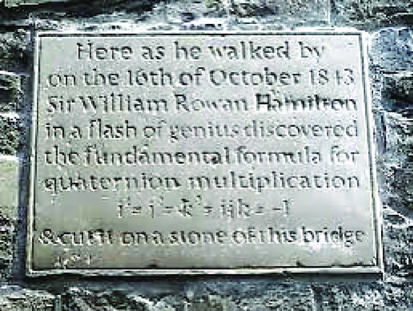
Figure 1: The quaternion plaque on Brougham Bridge, Dublin. From wikipedia https://en.wikipedia.org/wiki/History_of_quaternions

Hamilton employed quaternions to describe the 3D rotations. Essentially he used the spin-$\frac{1}{2}$ spinor representation: Consider a 3D rotation $R$ around the axis along the direction of $\hat{\Omega}$ and the rotation angle is $\gamma$. Define a unit imaginary quaternion,

$$\omega(\hat{\Omega})=i\sin\theta\cos\phi+j\sin\theta\sin\phi+k\cos\theta,$$ (10)

where $\theta$ and $\phi$ are the polar and azimuthal angles of $\hat{\Omega}$. Then a unit quaternion associated with such a rotation is defined as

$$q=\cos\frac{\gamma}{2}+\omega(\hat{\Omega})\sin\frac{\gamma}{2},$$ (11)

which is essentially an SU(2) matrix. A 3D vector $\vec{r}$ is mapped to an imaginary quaternion $r=xi+yj+zk$. After the rotation, $\vec{r}$ is transformed to $\vec{r}^{\prime}$, and its quaternion form is

$$r^{\prime}=qrq^{-1}.$$ (12)

This expression defines the homomorphism from SU(2) to SO(3). In fact, using quaternions to describe rotation is more efficient than using the 3D orthogonal matrix, hence, quaternions are widely used in computer graphics and aerospace engineering even today. If set $\vec{r}=\hat{z}$ in Eq. 12, and let $q$ run over unit quaternions, which span the $S^{3}$ sphere, then a mapping from $S^{3}$ to $S^{2}$ is defined as

$$n=qkq^{-1},$$ (13)

which is the 1st Hopf map.

Hamilton spent the last 20 years of his life to promote quaternions. His ambition was to invent quaternion analysis which could be as powerful as complex analysis. Unfortunately, this was not successful because of the non-commutative nature of quaternions. Nevertheless, Fueter found the analogy to the Cauchy-Riemann condition for quaternion analysis Sudbery (1979); Frenkel and Libine (2008). Consider a quaternionically valued function $f(x,y,z,u)$: It is quaternionic analytic if it satisfies the following Cauchy-Riemann-Fueter condition,

$$\frac{\partial f}{\partial x}+i\frac{\partial f}{\partial y}+j\frac{\partial f}{\partial z}+k\frac{\partial f}{\partial u}=0.$$ (14)

Eq. 14 is the left-analyticity condition since imaginary units are multiplied from the left. A right-analyticity condition can also be similarly defined in which imaginary units are multiplied from the right. The left one is employed throughout this article for consistency. For a quaternionic analytic function, the analogy to the Cauchy integral is

$$\frac{1}{2\pi^{2}}\oiiint\frac{1}{|q-q_{0}|^{2}(q-q_{0})}Dqf(q)=f(q_{0}),$$ (15)

where the integral is over a closed three-dimensional volume surrounding $q_{0}$. The measure of the volume element is,

$$D(q) = dy\wedge dz\wedge du-idx\wedge dz\wedge du$$ (16)

$$+ jdx\wedge dy\wedge du-kdx\wedge dy\wedge dz,$$

and $K(q)$ is the four-dimensional Green’s function,

$$K(q)=\frac{1}{q|q|^{2}}=\frac{x-yi-zj-uk}{(x^{2}+y^{2}+z^{2}+u^{2})^{2}}.$$ (17)

There have also been considerable efforts in formulating quantum mechanics and quantum field theory based on quaternions instead of complex numbers Finkelstein (1962); Adler (1995). Quaternions are also used to formulate the Laughlin-like wavefunctions in the 2D fractional quantum Hall physics Balatsky (1992).

As discussed in “Selected Papers (1945-1980) of Chen Ning Yang with Commentary” Yang (2005), C. N. Yang speculated that quaternion quantum theory would be a major revolution to physics, mostly based on the viewpoint of non-Abelian gauge theory. He wrote, “… I continue to believe that the basic direction is right. There must be an explanation for the existence of SU(2) symmetry: Nature, we have repeatedly learned, does not do random things at the fundamental level. Furthermore, the explanation is most likely in quaternion algebra: its symmetry is exactly SU(2). Besides, the quaternion algebra is a beautiful structure. Yes, it is noncommutative. But we have already learned that nature chose noncommutative algebra as the language of quantum mechanics. How could she resist using the only other possible nice algebra as the language to start all the complex symmetries that she built into the universe?”

III Complex analyticity and two-dimensional Landau level

In this section, I recapitulate the basic knowledge of the 2D Landau level problem, including both the non-relativistic Schrödinger equation in Sect. III.1 and the Dirac equation in Sect. III.2. I explain the complex analyticity of the 2D lowest Landau level wavefunctions.

III.1 2D Landau level for non-relativistic electrons

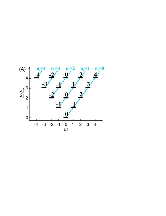
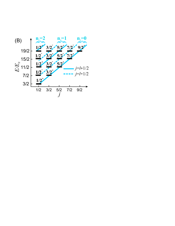
Figure 2: A) The energy level diagram of 2D harmonic oscillators v.s. the magnetic quantum number $m$. The states along the tilted lines are reorganized into the 2D flat Landau levels. B) The eigenstates of the 3D harmonic oscillator labeled by total angular momentum $j_{\pm}=l\pm\frac{1}{2}$ Following the tilted solid (dashed) lines, these states are reorganized into the 3D Landau level sates with the positive (negative) helicity for $H^{\pm}_{3D,symm}$, respectively. (From Ref.Li and Wu (2013)).

The reason that the 2D Landau level wavefunctions are so interesting is that their elegancy. The external magnetic field reorganizes harmonic oscillator wavefunctions to yield analytic properties. To be concrete, the Hamiltonian for a 2D electron moving in an external magnetic field $B$ reads,

$$H_{2D,sym}=\frac{(\vec{P}-\frac{q}{c}\vec{A})^{2}}{2M}.$$ (18)

In the symmetric gauge, i.e., $A_{x}=-\frac{1}{2}By$ and $A_{y}=\frac{1}{2}Bx$, the 2D rotational symmetry is explicit. The diamagnetic $A^{2}$-term gives rise to the harmonic potential, and the cross term becomes the orbital Zeeman term. Then Eq. 18 can be reformulated as

$$H_{2D,sym}=\frac{P_{x}^{2}+P_{y}^{2}}{2M}+\frac{1}{2}M\omega_{0}^{2}(x^{2}+y^{2})-\omega_{0}L_{z},$$ (19)

where $\omega_{0}$ is half of the cyclotron frequency $\omega_{c}$; $\omega_{c}=qB/(Mc)$ and $qB>0$ is assumed. Eq. 19 can also be interpreted as the Hamiltonian of a rotating 2D harmonic potential, which is how the Landau level Hamiltonian is realized in cold atom systems.

Since these the harmonic potential and orbital Zeeman term commute with each other, the Landau level wavefunctions are just wavefunctions of 2D harmonic oscillators. In Fig. 2 A), the spectra of the 2D harmonic oscillator v.s. the magnetic quantum number $m$ are plotted, exhibiting a linear dependence on $m$ as $E_{n_{r},m}=\hbar\omega_{0}(2n_{r}+m+1)$ where $n_{r}$ is the radial quantum number. If we view this diagram horizontally, they are with finite degeneracies exhibiting a trivial topology. But if they are viewed along the diagonal direction, they become Landau levels. This reorganization is due to the orbital Zeeman term, which also disperses linearly $E_{Z}=-m\hbar\omega_{0}$. It cancels the same linear dispersion of the 2D harmonic oscillator, such that the Landau level energies become flat. The wavefunctions of the lowest Landau level states with $n_{r}=0$ are $\psi_{LLL,m}(z)=z^{m}e^{-|z|^{2}/(4l_{B}^{2})}$ with $m\geq 0$, where the magnetic length $l_{B}=\sqrt{\hbar c/(qB)}$.

Now we impose the complex analyticity, i.e., the Cauchy-Riemann condition, to select a subset of harmonic oscillator wavefunctions. Physically it is implemented by the magnetic field. It just means that the cyclotron motion is chiral. After suppressing the Gaussian factor, the lowest Landau level wavefunction is simply,

$$\psi_{LLL}(z)=f(z),$$ (20)

which has a one-to-one correspondence to a complex analytic function. In fact, the complex analyticity greatly facilitated the construction of the many-body Laughlin wavefunctions Laughlin (1983),

$$\psi_{L}(z_{1},...,z_{n})=\Pi_{i<j}(z_{i}-z_{j})^{3}e^{-\sum_{i}\frac{|z_{i}|^{2}}{4l^{2}_{b}}},$$ (21)

which is actually analytic in terms of multi-complex variables.

Along the edge of a 2D Landau level system, the bulk flat states change to 1D dispersive chiral edge modes. They satisfy the chiral wave equation Girvin (1999),

$$\Big{(}\frac{1}{v_{f}}\frac{\partial}{\partial t}-\frac{\partial}{\partial x}\Big{)}\psi(x,t)=0,$$ (22)

where $v_{f}$ is the Fermi velocity.

III.2 2D Landau level for Dirac fermions

The is essentially a square-root problem of the Landau level Hamiltonian of a Schrödinger fermion in Eq. 18. The Hamiltonian reads Semenoff (1984),

$$H^{D}_{2D}=l_{0}\omega\Big{\{}(p_{x}-A_{x})\sigma_{x}+(p_{y}-A_{y})\sigma_{y}\Big{\}},$$ (23)

where $A_{x}=-\frac{1}{2}By$, $A_{y}=\frac{1}{2}Bx$, $l_{0}=\sqrt{\frac{2\hbar c}{|qB|}}$, and $\omega=\frac{|qB|}{2mc}$. It can be recast in the form of

$$H_{2D}^{D}=\frac{\hbar\omega}{\sqrt{2}}\left[\begin{array}[]{cc}0&a_{y}^{\dagger}+ia_{x}^{\dagger}\\ a_{y}-ia_{x}&0\end{array}\right],$$ (26)

where $a_{i}=\frac{1}{\sqrt{2}}(x_{i}/l_{0}+ip_{i}l_{0}/\hbar)$ $(i=x,y)$ are the phonon annihilation operators.

The square of Eq. 26 is reduced to the Landau level Hamiltonian of a Schrödinger fermion with a supersymmetric structure as

$$(H_{2D}^{D})^{2}/(\frac{1}{2}\hbar\omega)=\left[\begin{array}[]{cc}H_{2D,sym}-\frac{1}{2}\hbar\omega&0\\ 0&H_{2D,sym}+\frac{1}{2}\hbar\omega\end{array}\right],$$ (29)

where $H_{2D,sym}$ is given in Eq. 19. The spectra of Eq. 26 are $E_{\pm n}=\pm\sqrt{n}\hbar\omega$ where $n$ is the Landau level index. The zeroth Landau level states are singled out: Only the upper component of their wavefunctions is nonzero,

$$\Psi_{2D,LLL}^{D}(z)=\left(\begin{array}[]{c}\psi_{LLL}(z)\\ 0\end{array}\right).$$ (33)

$\psi_{LLL}(z)$ is the 2D lowest Landau level wavefunctions of the Schrödinger equation, which is complex analytic. Other Landau levels with positive and negative energies distribute symmetrically around the zero energy.

Due to the particle-hole symmetry, each state of the zeroth Landau level is a half-fermion Jackiw-Rebbi mode Jackiw and Rebbi (1976); Heeger et al. (1988). When the chemical potential $\mu$ approaches $0^{\pm}$, the zeroth Landau level is fully occupied, or, empty, respectively. The corresponding electromagnetic response is,

$$j_{\mu}=\pm\frac{1}{8\pi}\frac{q^{2}}{\hbar}\epsilon_{\mu\nu\lambda}F_{\nu\lambda},$$ (34)

known as the 2D parity anomaly Redlich (1984a, b); Semenoff (1984); Niemi and Semenoff (1986), where $\pm$ refer to $\mu=0^{\pm}$, respectively. The two spatial components of Eq. 34 are just the half-quantized quantum Hall conductance, and the temporal component is the half-quantized Streda formula Streda (1982).

IV 3D Landau level and quaternionic analyticity

We have seen the close connection between complex analyticity and 2D topological states. In this section, we discuss how to construct high-dimensional topological states in flat spaces based on quaternionic analyticity.

IV.1 3D Landau level Hamiltonian

Our strategy is based on high-dimensional harmonic oscillator wavefunctions. Again we need to select a subset of them for non-trivial topological properties: The selection criterion is quaternionic analyticity, and physically it is imposed by spin-orbit coupling. The physical picture of the 3D Landau level wavefunctions in the symmetric-like gauge is intuitively presented in Fig. 3 (A). It generalizes the fixed complex plane in the 2D Landau level problem to a moving frame embedded in 3D. Define a frame with the orthogonal axes $\hat{e}_{1}$, $\hat{e}_{2}$, and $\hat{e}_{3}$, and the complex analytic wavefunctions are defined in the $\hat{e}_{1}$-$\hat{e}_{2}$ plane with spin polarized along the $\hat{e}_{3}$ direction. Certainly this frame can be rotated to an arbitrary configuration. The same strategy can be applied to any high dimensions.

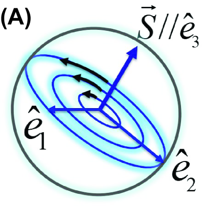
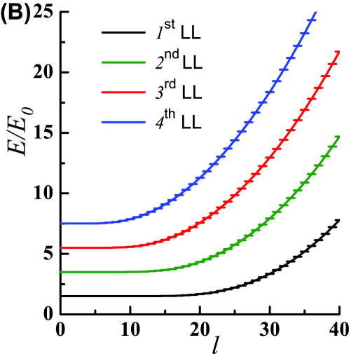
Figure 3: A) The coherent state picture for 3D lowest Landau level wavefunctions based on Eq. 37. $\hat{e}_{1}$-$\hat{e}_{2}$-$\hat{e}_{3}$ form an orthogonal triad. The lowest Landau level wavefunction is complex analytic in the orbital plane $\hat{e}_{1}$-$\hat{e}_{2}$ and spin is polarized along $\hat{e}_{3}$. B) The surface spectra for the 3D Landau level Hamiltonian Eq.35. The open boundary condition is used for a ball with the radius $R_{0}/l_{so}=8$. (From Ref. Li and Wu (2013).)

Now we present the 3D Landau level Hamiltonian as constructed in Ref. Li and Wu (2013). Consider to couple a spin-$\frac{1}{2}$ fermion to the 3D isotropic SU(2) Aharanov-Casher potential $\vec{A}=\frac{G}{2}\vec{\sigma}\times\vec{r}$ where $G$ is the coupling constant and $\vec{\sigma}$’s are the Pauli matrices. The resultant Hamiltonian is

$$H^{\pm}_{3D,sym} = \frac{1}{2M}\big{(}\vec{P}-\frac{q}{c}\vec{A}(\vec{r})\big{)}^{2}+V(\vec{r})$$ (35)

$$= \frac{P^{2}}{2M}+\frac{1}{2}M\omega_{0}^{2}r^{2}\mp\omega_{0}\vec{\sigma}\cdot\vec{L},$$

where $\pm$ refer to $G>0~{}(<0)$, respectively; $\omega_{0}=\frac{1}{2}\omega_{so}$ and $\omega_{so}=|qG|/(Mc)$ is the analogy of the cyclotron frequency. $V(r)=-\frac{1}{2}M\omega_{0}^{2}r^{2}$, nevertheless, the $\frac{1}{2M}(\frac{q}{c})^{2}A^{2}(r)$ term in the kinetic energy contributes a quadratic scalar potential which equals $2|V(r)|$, hence, Eq. 35 is still bound from below. In contrast to the 2D case, $H^{\pm}_{3D,sym}$ preserve time-reversal symmetry. It can also be formulated as a 3D harmonic potential plus a spin-orbit coupling term. Again since these two terms commute, the 3D Landau level wavefunctions are just the eigenstates of a 3D harmonic oscillator.

Consider the eigenstates of a 3D harmonic oscillator with an additional spin degeneracy $\uparrow$ and $\downarrow$. For later convenience, their eigenstates are organized into the bases of the total angular momentum $j_{\pm}=l\pm\frac{1}{2}$, where $\pm$ represent the positive and negative helicities, respectively. The corresponding spectra are plotted in Fig. 2 (B), showing a linear dispersion with respect to $l$ as $E_{n_{r},J_{\pm}=l\pm\frac{1}{2},J_{z}}=\hbar\omega_{0}(2n_{r}+l+\frac{3}{2})$.

Again, if we view the spectra along the diagonal direction, the novel topology appears. The spin-orbit coupling term $\vec{\sigma}\cdot\vec{k}$ has two branches of eigenvalues, both of which disperse linearly with $l$ as $l\hbar$ and $-(l+1)\hbar$ for the positive and negative helicity sectors, respectively. Combining the harmonic potential and spin-orbit coupling, we arrive at the flat Landau levels: For $H^{+}_{3D}$, the positive helicity states become dispersionless with respect to $j_{+}$ , a main feature of Landau levels. Similarly, the negative helicity states become flat for $H^{-}_{3D}$. States in the 3D Landau level show the same helicity.

IV.2 The SU(2) group manifold for the lowest Landau level wavefunctions

Having understood why the spectra are flat, now we provide an intuitive picture for the lowest Landau level wavefunctions with the positive helicity. If expressed in the orthonormal basis of $(j\pm,j_{z})$, they are rather complicated,

$$\psi_{LLL,j_{+}=l+\frac{1}{2},j_{z}}(r,\hat{\Omega})=r^{l}Y_{j_{+}=l+\frac{1}{2},j_{z}}(\hat{\Omega})e^{-\frac{r^{2}}{4l_{so}^{2}}},$$ (36)

where $l_{so}=\sqrt{\hbar c/|qG|}$ is the analogy of the magnetic length and $Y_{j_{+}=l+\frac{1}{2},j_{z}}(\hat{\Omega})$ is the spin-orbit coupled spherical harmonic function.

Instead, they become very intuitive in the coherent state representation. Let us start with the highest weight states with $j_{+}=j_{z}$, whose wavefunctions are $\psi_{LLL,j_{+}=j_{z}}(r,\hat{\Omega})=(x+iy)^{l}\exp\{-\frac{r^{2}}{4l_{so}^{2}}\}\otimes|\uparrow\rangle$. Their spins are polarized along the $z$-direction and orbital parts are complex analytic in the $xy$ plane. We then perform a general SU(2) rotation such that the $xyz$-frame is rotated to the frame of $\hat{e}_{1}$-$\hat{e}_{2}$-$\hat{e}_{3}$. For a coordinate vector $\vec{r}$, its projection in the $\hat{e}_{1}$-$\hat{e}_{2}$ plane forms a complex variable $\vec{r}\cdot(\hat{e}_{1}+i\hat{e}_{2})$ based on which we construct complex analytic functions. Now it is clear why spin-orbit coupling is essential. Otherwise, if the plane is flipped, then the complex variable changes to its conjugate, and the complex analyticity is lost. Nevertheless, since spin is polarized perpendicular to the $\hat{e}_{1}$-$\hat{e}_{2}$-plane, spin also flips during the flipping of the orbital plane, such that the helicity remains invariant. In general, we can perform an arbitrary $SU(2)$ rotation on the highest weight states and arrive at a set of coherent states forming the over-complete bases of the lowest Landau level states as

$$\psi_{LLL,\hat{e}_{1,2,3},j_{+}}(r,\hat{\Omega})=[(\hat{e}_{1}+i\hat{e}_{2})\cdot\vec{r}]^{l}e^{-\frac{r^{2}}{4l_{so}^{2}}}\otimes|\alpha_{\hat{e}_{3}}\rangle,(l\geq 0)$$

(37)

where $(\hat{e}_{3}\cdot\vec{\sigma})|\alpha_{\hat{e}_{3}}\rangle=|\alpha_{\hat{e}_{3}}\rangle$.

Now we can make a comparison among harmonic oscillator wavefunctions in different dimensions.

1. In 1D, we only have the real Hermite polynomials.

2. In 2D, a subset of harmonic wavefunctions $z^{m}$ (lowest Landau level) are selected exhibiting the $U(1)$ structure.

3. In 3D, the complex plane $\hat{e}_{1}$-$\hat{e}_{2}$ associated with the frame $\hat{e}_{1}$-$\hat{e}_{2}$-$\hat{e}_{3}$ are floating. This is similar to the rigid-body configuration. In other words, the configuration space of the 3D lowest Landau level states is that of a triad, or, the $SU(2)$ group manifold.

Since the SU(2) group manifold is isomorphic to the space of unit quaternions, this motivates us to consider the analytic structure in terms of quaternions, which will be presented in Sect. IV.4.

IV.3 The off-centered solutions to the lowest Landau level states

Different from the 2D Landau level Hamiltonian, which possesses the magnetic translation symmetry, the 3D one of Eq. 35 does not possess such a symmetry due to the non-Abelian nature of the SU(2) gauge potential. Nevertheless, based on the coherent states described by Eq. 37, we can define magnetic translations within the $\hat{e}_{1}$-$\hat{e}_{2}$ plane, and organize the off-centered solutions in the lowest Landau level.

Consider all the coherent states in the $\hat{e}_{1}$-$\hat{e}_{2}$ plane described by Eq. 37. We define the magnetic translation for this set of states as

$$T_{\hat{e}_{3}}(\vec{\delta})=\exp[-\vec{\delta}\cdot\vec{\nabla}+\frac{i}{4l_{so}^{2}}~{}\vec{r}_{12}\cdot(\hat{e}_{3}\times\vec{\delta})],$$ (38)

where the translation vector $\vec{\delta}$ lies in the $\hat{e}_{1,2}$-plane and $\vec{r}_{12}=\vec{r}-\hat{e}_{3}(\vec{r}\cdot\hat{e}_{3})$. Set $\hat{e}_{1}=\hat{z}$, and the normal vector $\hat{e}_{3}$ lying in the $xy$-plane with an azimuthal angle $\phi^{\prime}$, i.e., $\hat{e}_{3}(\phi^{\prime})=\hat{x}\cos\phi^{\prime}+\hat{y}\sin\phi^{\prime}$, then $\alpha_{\hat{e}_{3}}(\phi^{\prime})=\frac{1}{\sqrt{2}}(|\uparrow\rangle+e^{i\phi^{\prime}}|\downarrow\rangle)$. Consider the lowest Landau level states localized at the origin,

$$\psi_{l=0,\hat{e}_{3}}(r,\hat{\Omega})=e^{-\frac{r^{2}}{4l_{so}^{2}}}\otimes|\alpha_{\hat{e}_{3}}\rangle,$$ (39)

and translate it along $\hat{z}$ at the distance $R$. According to Eq. 38, we arrive at

$$\psi_{\phi^{\prime},R}(\rho,\phi,z)=e^{i\frac{1}{2l_{so}^{2}}R\rho\sin(\phi-\phi^{\prime})}e^{-|\vec{r}-R\hat{z}|^{2}/4l_{so}^{2}}\otimes\alpha_{\hat{e}_{3}}(\phi^{\prime}),~{}$$ (40)

where $\rho=\sqrt{x^{2}+y^{2}}$ and $\phi$ is the azimuthal angular of $\vec{r}$ in the $xy$-plane.

Now we can restore the rotational symmetry around the $\hat{z}$-axis by performing the Fourier transform with respect to the angle $\phi^{\prime}$, i.e., $\psi_{j_{z}=m+\frac{1}{2},R}(\rho,\phi,z)=\int_{0}^{2\pi}\frac{d\phi^{\prime}}{2\pi}e^{im\phi^{\prime}}\psi_{\phi^{\prime},R}$. We arrive at the eigenstates of $j_{z}$ as

$$\psi_{j_{z}=m+\frac{1}{2},R}(\rho,\phi,z) = e^{\frac{-|\vec{r}-R\hat{z}|^{2}}{4l_{so}^{2}}}e^{im\phi}\Big{\{}J_{m}(x)|\uparrow\rangle$$ (41)

$$+ J_{m+1}(x)e^{i\phi}|\downarrow\rangle\Big{\}},$$

where $x=R\rho/(2l_{so}^{2})$. It describes a wavefunction with the shape of an ellipsoid, whose distribution in the $xy$-plane is within the distance of $ml_{so}^{2}/R$. The narrowest states $\psi_{\pm\frac{1}{2},R}$ have an aspect ratio scaling as $l_{so}/R$ when $R$ goes large. On the other hand, for those states with $|m|<R/l_{so}$, they localize within the distance of $l_{so}$ from the center located at $R\hat{z}$. As a result, the real space local density of states of the lowest Landau level grows linearly with $R$.

IV.4 Quaternionic analyticity of the lowest Landau level wavefunctions

In analogy to complex analyticity of the 2D lowest Landau level states, we have found that the helicity structure of the 3D lowest Landau levels leads to quaternionic analyticity.

Just like two real numbers forming a complex number, a two-component complex spinor $\psi=(\psi_{\uparrow},\psi_{\downarrow})^{T}$ can be mapped to a quaternion by multiplying a $j$ to the 2nd component

$$f=\psi_{\uparrow}+j\psi_{\downarrow}.$$ (42)

Then the familiar symmetry transformations can be represented via multiplying quaternions. The time-reversal transformation $i\sigma_{2}\psi^{*}$ becomes $Tf=-fj$ satisfying $T^{2}=-1$. The $U(1)$ phase $e^{i\theta}\to fe^{i\theta}$, and the SU(2) rotation becomes

$$e^{i\frac{\phi}{2}\sigma_{x}}\psi\to e^{k\frac{\phi}{2}}f,\ \ \,e^{i\frac{\phi}{2}\sigma_{y}}\psi\to e^{j\frac{\phi}{2}}f,\ \ \,e^{i\frac{\phi}{2}\sigma_{z}}\psi\to e^{-i\frac{\phi}{2}}f.$$

To apply the Cauchy-Riemann-Fueter condition Eq. 15 to 3D, we simply suppress the 4th coordinate,

$$\frac{\partial f}{\partial x}+i\frac{\partial f}{\partial y}+j\frac{\partial f}{\partial z}=0.$$ (44)

We prove a remarkable property below that this condition (Eq. 44) is rotationally invariant.

Lemma 1

If a quaternionic wavefunction $f(x,y,z)$ is quaternionic analytic, i.e., it satisfies the Cauchy-Riemann-Futer condition, then after an arbitrary rotation, the consequential wavefunction $f^{\prime}(x,y,z)$ remains quaternionic analytic.

Proof: Consider an arbitrary SU(2) rotation $g(\alpha,\beta,\gamma)=e^{-i\frac{\alpha}{2}\sigma_{z}}e^{-i\frac{\beta}{2}\sigma_{y}}e^{-i\frac{\gamma}{2}\sigma_{z}}$, where $\alpha,\beta,\gamma$ are Eulerian angles. In the quaternion representation, it maps to $g=e^{i\frac{\alpha}{2}}e^{-j\frac{\beta}{2}}e^{i\frac{\gamma}{2}}$. After this rotation $f(x,y,z)$ transforms to

$$f^{\prime}(x,y,z)=e^{i\frac{\alpha}{2}}e^{-j\frac{\beta}{2}}e^{i\frac{\gamma}{2}}f(x^{\prime},y^{\prime},z^{\prime}),$$ (45)

where $(x^{\prime},y^{\prime}$, $z^{\prime})$ are the coordinates by applying $g^{-1}$ on $(x,y,z)$. It can be checked that

$$\Big{(}\frac{\partial}{\partial x}+i\frac{\partial}{\partial y}+j\frac{\partial}{\partial z}\Big{)}e^{i\frac{\alpha}{2}}e^{-j\frac{\beta}{2}}e^{i\frac{\gamma}{2}}$$ (46)

$$= e^{i\frac{\alpha}{2}}e^{-j\frac{\beta}{2}}e^{i\frac{\gamma}{2}}\Big{(}\frac{\partial}{\partial x^{\prime}}+i\frac{\partial}{\partial y^{\prime}}+j\frac{\partial}{\partial z^{\prime}}\Big{)}.$$

Then we have

$$(\frac{\partial}{\partial x}+i\frac{\partial}{\partial y}+j\frac{\partial}{\partial z})f^{\prime}(x,y,z)=0.$$ (47)

Hence, the Cauchy-Riemann-Fueter condition is rotationally invariant.   

Based on this lemma, we prove the quaternionic analyticity of the 3D lowest Landau level wavefunctions.

Theorem 1

The 3D lowest Landau level wavefunctions of $H^{+}_{3D,sym}$ in Eq. 35 have a one-to-one correspondence to the quaternionic analytic polynomials in 3D.

Proof: We denote the quaternionic polynomials, which correspond to the orthonormal bases of the lowest Landau level wavefunctions in Eq. 36, as $f^{LLL}_{j_{+},j_{z}}$ with $j_{+}=l+\frac{1}{2}$, and $-j_{+}\leq j_{z}\leq j_{+}$. The highest weight states $f^{LLL}_{j_{+},j_{+}}=(x+iy)^{l}$ are complex analytic in the $xy$-plane, hence, it is obviously quaternionic analytic. Since all the coherent states can be obtained from the highest weight states via rotations, they are also quaternionic analytic. The coherent states form a set of overcomplete basis of the lowest Landau level wavefunctions, hence all the lowest Landau level wavefunctions are quaternionic analytic.

Next we prove the completeness that $f^{LLL}_{j_{+},j_{z}}$’s form the complete basis of the quaternoinic analytic polynomials in 3D. By counting the degrees of freedom of the $l$-th order polynomials of $x,y,z$, and the number of the constraints from Eq. 15, we calculate the total number of the linearly independent $l$-th order quaternionic analytic polynomials as $C^{2}_{l+2}-C^{2}_{l+1}=l+1$. On the other hand, any lowest Landau level state in the sector of $j_{+}=l+\frac{1}{2}$ can be represented as

$$f_{l}(x,y,z)=\sum_{m=0}^{l}f^{LLL}_{j_{+}=l+\frac{1}{2},j_{z}=m+\frac{1}{2}}q_{m},$$ (48)

where $q_{m}$ is a quaternion constant coefficient. Please note that $q_{lm}$’s are multiplied from right due to the non-commutativity of quaternions. In Eq. 48, we have taken into account the fact $f^{LLL}_{j_{+},-j_{z}}=-f^{LLL}_{j_{+},-j_{z}}j$ due to the time-reversal transformation. Hence, the degrees of freedom in the lowest Landau level with $j_{+}=l+\frac{1}{2}$ is also $l+1$. Hence, the lowest Landau level wavefunctions are complete for quaternionic analytic polynomials.   

IV.5 Generalizations to 4D and above

The above procedure can be straightforwardly generalized to four and even higher dimensions. To proceed, we need to employ the Clifford algebra $\Gamma$-matrices. Their ranks in different dimensions and concrete representations are presented in Appendix A. Then we use the $N$-D harmonic oscillator potential combined with spin-orbit coupling as

$$H^{ND,LL}=\frac{p_{ND}^{2}}{2m}+\frac{1}{2}m\omega_{0}^{2}r_{ND}^{2}-\omega_{0}\sum_{1\leq i<j\leq N}\Gamma_{ij}L_{ij},$$ (49)

where $L_{ij}=r_{i}p_{j}-r_{j}p_{i}$. The spectra of Eq. 49 were studied in the context of the supersymmetric quantum mechanics Bagchi (2001). However, its connection with Landau levels was not noticed there. The spin operators in $N$-dimensions are defined as $\frac{1}{2}\Gamma_{ij}$.

For the 4D case, the minimal representations for the $\Gamma$-matrices are still two-dimensional. They are defined as

$$\Gamma_{ij}=-\frac{i}{2}[\sigma_{i},\sigma_{j}],\ \ \,\Gamma_{i4}=\pm\sigma_{i},$$ (50)

with $1\leq i<j\leq 3$. The $\pm$ signs of $\Gamma^{i4}$ correspond to two complex conjugate irreducible fundamental spinor representations of $SO(4)$, and the $+$ sign will be taken below. The spectra of the positive helicity states are flat as $E_{+,n_{r}}=(2n_{r}+2)\hbar\omega$. The coherent state picture for the 4D lowest Landau levels can be similarly constructed as follows: Again pick up two orthogonal axes $\hat{e}$ and $\hat{f}$ to form a 2D complex plane, and define complex analytic functions therein as,

$$(x_{a}\hat{e}_{a}+ix_{a}\hat{f}_{a})^{l}e^{-\frac{r^{2}}{4l_{so}^{2}}}\otimes|\alpha_{\hat{e},\hat{f}}\rangle,$$ (51)

where $|\alpha_{\hat{e},\hat{f}}\rangle$ is the eigenstate of $\Gamma^{\hat{e},\hat{f}}=\hat{e}_{a}\hat{f}_{b}\Gamma^{ab}$ satisfying

$$\Gamma^{\hat{e},\hat{f}}|\alpha_{\hat{e},\hat{f}}\rangle=|\alpha_{\hat{e},\hat{f}}\rangle.$$ (52)

Hence, its spin is locked with its orbital angular momentum in the $\hat{e}$-$\hat{f}$ plane.

Following similar methods in Sect. IV.4, we can prove that the 4D lowest Landau level wavefunctions for Eq. 49 satisfy the 4D Cauchy-Riemann-Futer condition Eq. 14, and thus are quaternionic analytic functions. Again it can be proved that they form the complete basis for quaternionic left-analytic polynomials in 4D. As for even higher dimensions, quaternions are not defined. Nevertheless, the picture of the complex analytic function defined in the moving frame still applies. If we still work in the spinor representation, we can express the lowest Landau level wavefunctions as $\psi_{LLL}(x_{i})=f_{LLL}(x_{i})e^{-\frac{r^{2}}{2l_{0}^{2}}}$, where each component of the spinor $f_{LLL}$ is a polynomial of $r_{i}$ $(1\leq i\leq N)$. To work out the analytic properties of $f_{LLL}$, we factorize Eq. 49 as

$$H^{ND,LL}=\hbar\omega_{0}\left(\Gamma^{i}a_{i}^{\dagger}\right)\left(\Gamma^{j}a_{j}\right),$$ (53)

where $a_{i}$ is the phonon operator in the $i$-th dimension defined as $a_{i}=\frac{1}{\sqrt{2}}\big{(}\frac{1}{l_{0}}r_{i}+i\frac{l_{0}}{\hbar}p_{i}\big{)}$, and $l_{0}=\sqrt{\frac{\hbar}{m\omega_{0}}}$. Then $f_{LLL}(x_{i})$ satisfies the following equation,

$$\Gamma^{j}\frac{\partial}{\partial x_{j}}f_{LLL}(x_{i})=0,$$ (54)

which can be viewed as the Euclidean version of the Weyl equation. When coming back to 3D and 4D, and following the mapping Eq. 42, we arrive at quaternionic analyticity.

New let us construct the off-centered solutions to the lowest Landau level states in 4D. We use $\vec{r}$ to denote a point in the subspace of $x_{1}$-$x_{2}$-$x_{3}$, and $\hat{\Omega}$ as an arbitrary unit vector in it. Set $\hat{e}=\hat{\Omega}$ and $\hat{f}=\hat{e}_{4}$ (the unit vector along the 4th axis) in Eq. 51. $\alpha_{\hat{\Omega}\hat{e}_{4}}$ satisfies

$$(\sigma_{i4}\Omega_{i})\alpha_{\hat{\Omega}\hat{e}_{4}}=(\vec{\sigma}\cdot\hat{\Omega})\alpha_{\hat{\Omega}\hat{e}_{4}}=\alpha_{\hat{\Omega}\hat{e}_{4}},$$ (55)

hence,

$$\alpha_{\hat{\Omega}\hat{e}_{4}}=(\cos\frac{\theta}{2},\sin\frac{\theta}{2}e^{i\phi})^{T},$$ (56)

where we have used the gauge convention that the singularity is located at the south pole. Define the magnetic translation in the $\hat{\Omega}$-$\hat{e}_{4}$ plane,

$$T_{\hat{\Omega}x_{4}}(u_{0}\hat{x}_{4})=\exp\Big{(}-u_{0}\partial_{x_{4}}-\frac{i}{4l_{so}^{2}}(\vec{r}\cdot\hat{\Omega})u_{0}\Big{)},$$ (57)

which translates along the $\hat{e}_{4}$-axis at the distance of $u_{0}$. Apply this translation to the state of $e^{-r^{2}/4l_{so}^{2}}\otimes\alpha_{\hat{\Omega}\hat{e}_{4}}$, we arrive at the off-center solution

$$\psi_{\Omega,u_{0}}(\vec{r},x_{4})=e^{-\frac{r^{2}+x_{4}^{2}}{4l_{so}^{2}}}e^{-i\frac{ru_{0}}{2l_{so}^{2}}}\otimes\alpha_{\hat{\Omega}\hat{e}_{4}}.$$ (58)

Next, we perform the Fourier transform over the direction $\hat{\Omega}$,

$$\psi_{4D;j,j_{z}}(\vec{r},x_{4}) = \int d\Omega~{}Y_{-\frac{1}{2},l+\frac{1}{2},m+\frac{1}{2}}(\hat{\Omega})\psi_{\Omega,w_{0}}(\vec{r},x_{4}),\ \ \,\ \ \,$$ (59)

where $j=l+\frac{1}{2}$ and $j_{z}=m+\frac{1}{2}$. Due to the Berry phase structure $\alpha_{\hat{\Omega}\hat{e}_{4}}$ over $\hat{\Omega}$, monopole spherical harmonics, $Y_{-\frac{1}{2},l+\frac{1}{2},m+\frac{1}{2}}(\hat{\Omega})$, are used instead of the regular spherical harmonics. Then Eq. 59 possesses the 3D rotational symmetry around the new center $(0,0,0,w_{0})$, and Eq. 59 possesses with the good quantum numbers of 3D angular momentum $(j,j_{z})$. The monopole harmonic function $Y_{q;jj_{z}}(\hat{\Omega})$ here is defined as

$$Y_{q;jj_{z}}(\hat{\Omega})=\sqrt{\frac{2j+1}{4\pi}}e^{i(j_{z}+q)\phi}d^{l}_{j_{z},-q}(\theta),$$ (60)

where $\theta$ and $\phi$ are the polar and azimuthal angles of $\hat{\Omega}$, and $d^{l}_{j_{z},-q}(\theta)=\langle jj_{z}|e^{-iJ_{y}\theta}|j-q\rangle$ is the standard Wigner rotation $d$-matrix. The gauge choice is consistent with that of the Eq. 56.

IV.6 Boundary helical Dirac and Weyl modes

The topological nature of the 3D Landau level states exhibits clearly in the gapless surface spectra. Consider a ball of the radius $R_{0}\gg l_{so}$ imposed by the open boundary condition. We have numerically solved the spectra as shown in Fig. 3 (B). Inside the bulk, the Landau level spectra are flat with respect to $j_{+}=l+\frac{1}{2}$. As $l$ increases to large values such that the classic orbital radiuses approach the boundary, the Landau levels become surface states and develop dispersive spectra.

We can also derive the effective equation for the surface mode based on Eq. 35. Since $r$ is fixed at the boundary, it becomes a rotator equation on the sphere. By linearizing the dispersion at the chemical potential $\mu$, and replacing the angular momentum quantum number $l$ by the operator $\vec{\sigma}\cdot\vec{L}$, we arrive at $H_{sf}=(v_{f}/R_{0})\vec{\sigma}\cdot\vec{L}-\mu$ with $v_{f}$ the Fermi velocity. This is the helical Dirac equation defined on the boundary sphere. When expanded in the local patch around the north pole $R_{0}\hat{z}$, we arrive at

$$H_{sf}=\hbar v_{f}(\vec{k}\times\vec{\sigma})\cdot\hat{z}-\mu.$$ (61)

The gapless surface states are robust against time-reversal invariant perturbations if odd numbers of helical Fermi surfaces exist according to the $\mathbb{Z}_{2}$ criterion Kane and Mele (2005a, b). Since each fully occupied Landau level contributes one helical Dirac Fermi surface, the bulk is topologically nontrivial if odd numbers of Landau levels are occupied.

A similar procedure can be applied to the high-dimensional case by imposing the open boundary condition to Eq. 49. For example, around the north pole of $r_{N}=(0,....,R_{0})$, the linearized low energy equation for the boundary modes is

$$H_{bd}=\hbar v_{f}\sum_{i=1}^{D-1}k_{i}\Gamma^{iN}-\mu.$$ (62)

On the boundary of the 4D sphere, it becomes the 3D Weyl equation that

$$H_{bd}=\hbar v_{f}\vec{k}\cdot\vec{\sigma}-\mu.$$ (63)

IV.7 Bulk-boundary correspondence

	Bulk (Euclidean)	Boundary (Minkowski)
2D LLL	complex analyticity	1D chiral wave
	$\partial_{x}f+i\partial_{y}f=0$	$\partial_{t}\psi+\partial_{x}\psi=0$
3D LLL	(3D) quaternionic analyticity	2D helical Dirac mode
	$\partial_{x}f+i\partial_{y}f+j\partial_{z}f=0$	$\partial_{t}\psi+\sigma_{2}\partial_{x}\psi-\sigma_{1}\partial_{y}\psi=0$
4D LLL	quaternionic analyticity	3D Weyl mode
	$\partial_{x}f+i\partial_{y}f+j\partial_{z}f+k\partial_{u}f=0$	$\partial_{t}\psi+\sigma_{1}\partial_{x}\psi+\sigma_{2}\partial_{y}\psi+\sigma_{3}\partial_{z}\psi=0$

Table 1: Bulk-boundary correspondence in the lowest (LLL) states in 2, 3, and 4 dimensions.

We have already studied the bulk and boundary states of 2D, 3D and 4D lowest Landau level states. They exhibit a series of interesting bulk-boundary correspondences as summarized in Table I. In the 2D case, the bulk wavefunctions in the lowest Landau level is complex analytic satisfying the Cauchy-Riemann condition. The 1D edge states satisfy the chiral wave equation Eq. 22. It is essentially the Weyl equation, which is actually a single component equation in 1D. It can be viewed as the Minkowski version of the Cauchy-Riemann condition of Eq. 4. Or, conversely, the Cauchy-Riemann condition for the bulk wavefunctions can be viewed as the Euclidean version of the Weyl equation.

This correspondence goes in parallel in 3D and 4D lowest Landau level wavefunctions. Their bulk wavefunctions satisfy the quaternionic analytic conditions, which can be viewed as an Euclidean version of the helical Dirac and Weyl equations, respectively.

IV.8 Many-body interacting wavefunctions

It is natural to further investigate many-body interacting wavefunctions in the lowest Landau levels in 3D and 4D. As is well-known that the complex analyticity of the 2D lowest Landau level wavefunctions results in the elegant from of the 2D Laughlin wavefunction Eq. 21, which describes a 2D quantum liquid Laughlin (1983); Girvin (1999). It is natural to further expect that the quaternionic analyticity of the 3D and 4D lowest Landau levels would work as a guidance in constructing high-dimensional SU(2) invariant quantum liquid. Nevertheless, the major difficulty is that quaternions do not commute. It remains challenging how to use quaternions to represent a many-body wavefunction with the spin degree of freedom.

Nevertheless, we present below the spin polarized fractional many-body states in 3D and 4D Landau levels. In the 3D case, if the interaction is spin-independent, we expect spontaneous spin polarization at very low fillings due to the flatness of lowest Landau level states in analogy to the 2D quantum Hall ferromagnetism Lee and Kane (1990); Sondhi et al. (1993); Fertig et al. (1994); Read and Sachdev (1995); Girvin (1999). According to Eq. 37, fermions concentrate to the highest weight states in the orbital plane $\hat{e}_{1}$-$\hat{e}_{2}$ with spin polarized along $\hat{e}_{3}$, then it is reduced to a 2D quantum Hall-like problem on a membrane floating in the 3D space. Any 2D fractional quantum Hall-like state can be formed under suitable interaction pseudopotentials Haldane (1983); Haldane and Rezayi (1985); Prange and Girvin (1990). For example, the $\nu=\frac{1}{3}$ Laughlin-like state on this membrane is constructed as

$$\Psi_{\frac{1}{3}}(\vec{r}_{1},\vec{r}_{2},...,\vec{r}_{n})_{\sigma_{1}\sigma_{2}...\sigma_{n}}$$

$$= \prod_{i<j}[(\vec{r}_{i}-\vec{r}_{j})\cdot(\hat{e}_{1}+i\hat{e}_{2})]^{3}\otimes|\alpha_{\hat{e}_{3}}\rangle_{\sigma_{1}}|\alpha_{\hat{e}_{3}}\rangle_{\sigma_{2}}...|\alpha_{\hat{e}_{3}}\rangle_{\sigma_{n}},$$

where $|\alpha_{\hat{e}_{3}}\rangle$ represents a polarized spin eigenstate along $\hat{e}_{3}$, and the Gaussian weight is suppressed for simplicity. Such a state breaks rotational symmetry and time-reversal symmetry spontaneously, thus it possesses low energy spin-wave modes. Due to the spin-orbit locked configuration in Eq. 37, spin fluctuations couple to the vibrations of the orbital motion plane, thus the metric of the orbital plane becomes dynamic. This is a natural connection to the work of geometrical description in fractional quantum Hall states Haldane (2011); Can et al. (2014); Klevtsov et al. (2017).

Let us consider the 4D case, we assume that spin is polarized as the eigenstate $|\uparrow\rangle$ of $\Gamma^{12}=\Gamma^{34}=\sigma_{3}$. The corresponding spin-polarized lowest Landau level wavefunctions are expressed as

$$\Psi^{4D}_{LLL,m,n}=(x+iy)^{m}(z+iu)^{n}\otimes|\uparrow\rangle,$$ (65)

with $m,n\geq 0$. If all these spin polarized lowest Landau level states with $0\leq m<N_{m}$ and $0\leq n<N_{n}$ are filled, the many-body wavefunction is a Slater-determinant as

$$\Psi^{4D}(v_{1},w_{1};\cdots;v_{N},w_{N})=\det[v_{i}^{\alpha}w_{i}^{\beta}],$$ (66)

where the coordinates of the $i$-th particle form two pairs of complex numbers as $v_{i}=x_{i}+iy_{i}$ and $w_{i}=z_{i}+iu_{i}$; $\alpha$, $\beta$ and $i$ satisfy $0\leq\alpha<N_{m}$, $0\leq\beta<N_{n}$, and $1\leq i\leq N=N_{m}N_{n}$. Such a state has a 4D uniform density as $\rho=\frac{1}{4\pi^{4}l_{G}^{2}}$. A Laughlin-like wavefunction can be written down as $\Psi^{4D}_{k}=(\Psi^{4D})^{k}$ whose filling relative to $\rho$ should be $1/k^{2}$. It would be interesting to further study its electromagnetic responses and fractional topological excitations based on $\Psi^{4D}_{k}$. Again such a state spontaneously breaks rotational symmetry, and the coupled spin and orbital excitations would be interesting.

V Dimensional reductions: 2D and 3D Landau levels with broken parity

In this section, we review another class of isotropic Landau level-like states with time-reversal symmetry but broken parity in both 2D and 3D. The Hamiltonians are again harmonic potential plus spin-orbit coupling, but it is the coupling between spin and linear momentum, not orbital angular momentum Wu et al. (2011); Li et al. (2012a, 2016). They exhibit topological properties very similar to Landau levels.

An early study of these systems filled with bosons can be found in Ref. Wu and Mondragon-Shem (2008). The spin-orbit coupled Bose-Einstein condensations (BECs) spontaneously break time-reversal symmetry, and exhibit the skyrmion type spin textures coexisting with half-quantum vortices, which have been reviewed in Ref. Zhou et al. (2013). Spin-orbit coupled BECs have become an active research direction of cold-atom physics, as extensively studied in literature. Wu et al. (2011); Hu et al. (2012); Sinha et al. (2011); Ghosh et al. (2011); Wang et al. (2010); Ho and Zhang (2011).

V.1 The 2D parity-broken Landau levels

We consider the Hamiltonian of Rashba spin-orbit coupling combined with a 2D harmonic potential as

$$H_{2D,hm}=-\frac{\hbar^{2}\nabla^{2}}{2M}+\frac{1}{2}M\omega^{2}r^{2}-\lambda(-i\hbar\nabla_{x}\sigma_{y}+i\hbar\nabla_{y}\sigma_{x}),$$

(67)

where $\lambda$ is the spin-orbit coupling strength with the unit of velocity. Eq. 67 possesses the $C_{v\infty}$-symmetry and time-reversal symmetry.

We fill the system with fermions and work on its topological properties. There are two length scales. The trap length scale is defined as $l_{T}=\sqrt{\frac{\hbar}{M\omega}}$. If without the trap, the single particle states $\psi_{\pm}(\vec{k})$ are eigenstates of the helicity operator $\vec{\sigma}\cdot(\vec{k}\times\hat{z})$ with eigenvalues of $\pm 1$. Their spectra are $\epsilon_{\pm}(\vec{k})=\hbar^{2}(k\mp k_{0})^{2}/(2M)$, respectively. The lowest energy states are $\psi_{+}(\vec{k})$ located around a ring in momentum space with radius $k_{0}=M\lambda/\hbar$. This introduces a spin-orbit length scale as $l_{so}=1/k_{0}$. Then the ratio between these two length scales defines a dimensionless parameter $\alpha=l_{T}/l_{so}$, which describes the spin-orbit coupling strength relative to the harmonic potential.

In the case of strong spin-orbit coupling, i.e., $\alpha\gg 1$, a clear picture appears in momentum space. The low energy states are reorganized from the plane-wave states $\psi_{+}(\vec{k})$ with $k\approx k_{0}$. Since $\alpha\gg 1$, we can safely project out the high energy negative helicity states $\psi_{-}(\vec{k})$, then the harmonic potential in the low energy sector becomes a Laplacian in momentum space coupled to a Berry connection $\vec{A}_{k}$ as

$$V=\frac{M}{2}\omega^{2}r^{2}=\frac{M}{2}\omega^{2}(i\nabla_{k}-A_{k})^{2},$$ (68)

which drives particle moving around the ring. It is well-known that for the Rashba Hamiltonian, the Berry connection $A_{k}$ gives rise to a $\pi$-flux at $\vec{k}=(0,0)$ but zero Berry curvature at $\vec{k}\neq 0$ Xiao et al. (2010). The consequence is that the angular momentum eigenvalues become half-integers as $j_{z}=m+\frac{1}{2}$. The angular dispersion of the spectra can be estimated as $E_{agl}(j_{z})=(j_{z}^{2}/2\alpha^{2})\hbar\omega$, which is strongly suppressed by spin-orbit coupling. On the other hand, the radial energy quantization remains as usual $E_{rad}(n_{r})=(n_{r}+\frac{1}{2})\hbar\omega$ up to a constant. Thus the total energy dispersion is

$$E_{n_{r},j_{z}}\approx\Big{(}n_{r}+\frac{1}{2}+\frac{j_{z}^{2}}{2\alpha^{2}}\Big{)}\hbar\omega.$$ (69)

Similar results have also been obtained in recent works of Ref. Hu et al. (2012); Sinha et al. (2011); Ghosh et al. (2011). Since $\alpha\gg 1$, the spectra are nearly flat with respect to $j_{z}$, we can treat $n_{r}$ as a Landau level index. The wavefunctions of Eq. 67 in the lowest Landau level with $n_{r}=0$ can be expressed in the polar coordinate as Eq. 71.

Next we define the edge modes of such systems, and their stability problem is quite different from that of the chiral edge modes of 2D magnetic Landau level systems. In the regime that $\alpha\gg 1$, the spin-orbit length $l_{so}$ is much shorter than $l_{T}$, such that $l_{T}$ is viewed as the cutoff of the sample size. States with $|j_{z}|<\alpha$ are viewed as bulk states which localize within the region of $r<l_{T}$. For states with $|J_{z}|\sim\alpha$, their energies touch the the bottom of the next higher Landau level, and thus they should be considered as edge states. Due to time-reversal symmetry, each filled Landau level of Eq. 67 gives rise to a branch of edge modes of Kramers’ doublets $\psi_{n_{r},\pm j_{z}}$. In other words, these edge modes are helical rather than chiral. Similarly to the $Z_{2}$ criterion in Ref. Kane and Mele (2005a, b), which was defined for Bloch wave states, in our case the following mixing term, $H_{mx}=\psi^{\dagger}_{2D,n_{r},j_{z}}\psi_{2D,n_{r},-j_{z}}+h.c.,$ is forbidden by time-reversal symmetry. Consequently, the topological index for this system is $Z_{2}$.

V.2 Dimensional reduction from 3D

In fact, we construct a Hamiltonian closely related to Eq. 67 such that its ground state is solvable exhibiting exactly flat dispersion. It is a consequence of dimensional reduction based on the 3D Landau level Hamiltonian Eq. 35. We cut a 2D off-centered plane perpendicular to the $z$-axis with the interception $z=z_{0}$. In this off-centered plane, inversion symmetry is broken, and Eq. 35 is reduced to

$$H_{2D,re} = H_{2D,hm}-\omega L_{z}\sigma_{z}.$$ (70)

The first term is just Eq. 67 by identifying $\lambda=\omega z_{0}$ and the frequency of the 2nd term is the same as that of the harmonic trap. If $z_{0}=0$, the Rashba spin-orbit coupling vanishes, and Eq.70 becomes the 2D quantum spin-Hall Hamiltonian, which is a double copy of Eq. 19. At $z_{0}\neq 0$, $\sigma_{z}$ is no longer conserved due to spin-orbit coupling.

In Sect. IV.3, we derived the off-centered ellipsoid type wavefunction in Eq. 41. After setting $z=z_{0}$ in Eq. 41, we arrive at the following 2D wavefunction,

$$\psi_{2D,j_{z}}(r,\phi) = e^{-\frac{r^{2}}{4l_{so}^{2}}}\Big{\{}e^{im\phi}J_{m}(k_{0}r)|\uparrow\rangle$$ (71)

$$+ e^{i(m+1)\phi}J_{m+1}(k_{0}r)|\downarrow\rangle\Big{\}},$$

where $J_{m}(k_{0}r)$’s are the Bessel functions. It is straightforward to prove that the simple reduction indeed gives rise to the solutions to the lowest Landau levels for Eq. 70, since the partial derivative along the $z$-direction of the solution in Eq. 41 equal zero at $z=z_{0}$. We also derive that the energy dispersion is exactly flat as,

$$H_{2D,re}~{}\psi_{2D,j_{z}}=\Big{(}1-\frac{\alpha^{2}}{2}\Big{)}\hbar\omega~{}\psi_{2D,j_{z}}.$$ (72)

The above two Hamiltonians Eq. 70 and Eq. 67 are nearly the same except the $L_{z}\sigma_{z}$ term, whose effect relies on the distance from the origin. Consider the lowest Landau level solutions at $\alpha\gg 1$. The decay length of the Gaussian factor is $l_{T}$. Nevertheless, the Bessel functions peak around $k_{0}r_{0}\approx m$, i.e., $r_{0}\approx\frac{m}{\alpha}l_{T}$. Hence for states with $j_{z}<\alpha$, their wavefunctions already decay before reach $l_{T}$. Then the $L_{z}\sigma_{z}$-term compared to the Rashba one is a small perturbation at the order of $\omega r_{0}/\lambda=r_{0}/z_{0}\ll 1$. In this regime, these two Hamiltonians are equivalent. In contrast, in the opposite limit that $j_{z}\gg\alpha^{2}$, the Bessel functions are cut off by the Gaussian factor, and only their initial power-law parts participate, and the classic orbit radiuses are just $r_{0}\approx\sqrt{m}l_{T}$, then the physics of Eq. 70 is controlled by the $L_{s}\sigma_{z}$-term as in the quantum spin Hall systems. For the intermediate region that $\alpha<j_{z}<\alpha^{2}$, the physics is a crossover between the above two limits.

The many-body physics based on the above spin-orbit coupled Landau levels in Eq. 71 would be very interesting. Fractional topological states would be expected which are both rotationally and time-reversal invariant. However, $s_{z}$ is not a good quantum number and party is also broken, hence, these states should be very different from a double copy of fractional Laughlin states with spin up and down particles. The nature of topological excitations and properties of edge modes will be deferred to a future study.

V.3 The 3D parity-broken Landau levels

We have also considered the problem of 3D harmonic potential plus a Weyl-type spin-orbit coupling as Li et al. (2012a),

$$H_{3D,hm}=-\frac{\hbar^{2}\nabla^{2}}{2M}+\frac{1}{2}M\omega^{2}r^{2}-\lambda(-i\hbar\vec{\nabla}\cdot\vec{\sigma}).$$ (73)

The analysis can be performed in parallel to the 2D case. In the absence of spin-orbit coupling, the low energy states of Eq. 73 in momentum space form a spin-orbit sphere. The harmonic potential further quantizes the energy spectra as

$$E_{n_{r},j,j_{z}}\approx\big{(}n_{r}+\frac{1}{2}+\frac{j(j+1)}{2\alpha^{2}}\big{)}\hbar\omega,$$ (74)

where $n_{r}$ is the Landau level index and $j$ is the total angular momentum. Again $j$ takes half-integer values because the Berry phase on the low energy sphere exhibits a unit monopole structure.

Now we perform the dimensional reduction from the 4D Hamiltonian Eq. 49 to 3D. We cut a 3D off-centered hyper-plane perpendicular to the 4-th axis with the interception $x_{4}=u_{0}$. Within this 3D hyper-plane of $(x_{1},x_{2},x_{3},x_{4}=u_{0})$, Eq. 49 is reduced to

$$H_{3D,re}=H_{3D,hm}-\omega\vec{L}\cdot\vec{\sigma},$$ (75)

where the first term is just Eq. 73 with the spin-orbit coupling strength set by $\lambda=\omega u_{0}$. Again, based on the center-shifted wavefunction in the lowest Landau level Eq. 59, and by setting $x_{4}=u_{0}$, we arrive at the following wavefunction

$$\psi_{3D,JJ_{z}}(\vec{r}) = e^{-\frac{r^{2}}{4l_{so}^{2}}}\Big{\{}j_{l}(k_{0}r)Y_{+,J,J_{z}}(\Omega_{r})$$ (76)

$$+ ij_{l+1}(k_{0}r)Y_{-,J,J_{z}}(\Omega_{r})\Big{\}},$$

where $k_{0}=u_{0}/l_{T}^{2}=m\lambda/\hbar$; $j_{l}$ is the $l$-th order spherical Bessel function. $Y_{\pm,j,l,j_{z}}$’s are the spin-orbit coupled spherical harmonics defined as

$$Y_{+,j,l,j_{z}}(\Omega)=\Big{(}\sqrt{\frac{l+m+1}{2l+1}}Y_{lm},\sqrt{\frac{l-m}{2l+1}}Y_{l,m+1}\Big{)}^{T}$$

with the positive eigenvalue of $l\hbar$ for $\vec{\sigma}\cdot\vec{L}$, and

$$Y_{-,j,l,j_{z}}(\Omega)=\Big{(}-\sqrt{\frac{l-m}{2l+1}}Y_{lm},\sqrt{\frac{l+m+1}{2l+1}}Y_{l,m+1}\Big{)}^{T}$$

with the negative eigenvalue of $-(l+1)\hbar$ for $\vec{\sigma}\cdot\vec{L}$. It is straightforward to check that $\psi_{3D,j,j_{z}}(\vec{r})$ in Eq. 76 is the ground state wavefunction satisfying

$$H_{3D,re}\psi_{3D,j,j_{z}}(\vec{r})=\Big{(}\frac{3}{2}-\frac{\alpha^{2}}{2}\Big{)}\hbar\omega\psi_{3D,j,j_{z}}(\vec{r}).$$ (77)

VI High-dimensional Landau levels of Dirac fermions

In this section, we review the progress on the study of 3D Landau levels of relativistic Dirac fermions Li et al. (2012b). This is a square-root problem of the 3D Landau level problem of Schrödinger fermions reviewed in Sect. IV. This can also be viewed of Landau levels of complex quaternions.

VI.1 3D Landau levels for Dirac fermions

In Eq. 26, two sets of phonon creation and annihilation operators $(a_{x},a_{y};a_{x}^{\dagger},a_{y}^{\dagger})$ are combined with the real and imaginary units to construct Landau level Hamiltonian for 2D Dirac fermions. Science in 3D there exist three sets of phonon creation and annihilation operators, complex numbers are insufficient.

The new strategy is to employ Pauli matrices $\vec{\sigma}$ such that

$$H_{3D}^{D} = v\Big{\{}\alpha_{i}p_{i}+\gamma_{i}i\hbar\frac{r_{i}}{l_{0}^{2}}\Big{\}}=\frac{\hbar\omega}{\sqrt{2}}\left[\begin{array}[]{cc}0&i\sigma_{i}a_{i}^{\dagger}\\ -i\sigma_{i}a_{i}&0\end{array}\right],\ \ \,$$ (80)

where the repeated index $i$ runs over $x,y$ and $z$; $v_{F}=\frac{1}{2}l_{0}\omega$. The convention of $\gamma$-matrices is

$$\beta=\gamma_{0}=\tau_{3}\otimes I,\ \ \,\alpha_{i}=\tau_{1}\otimes\sigma_{i},\ \ \,\gamma_{i}=\beta\alpha_{i}=i\tau_{2}\otimes\sigma_{i}.$$ (81)

Eq. 80 contains the complex combination of momenta and coordinates, thus it can be viewed as the generalized Dirac equation defined in the phase space. Apparently, Eq. 80 is rotationally invariant. It is also time-reversal invariant with the definition $T=\gamma_{2}\gamma_{3}K$ where $K$ is the complex conjugation, and $T^{2}=-1$. Since $\beta H_{3D}^{D}\beta=-H_{3D}^{D}$, $H_{3D}^{D}$ possesses the particle-hole symmetry and its spectra are symmetric with respect to the zero energy.

Similar to the 2D case, $(H^{D}_{3D})^{2}$ has a supersymmetric structure. The square of Eq. 80 is block-diagonal, and two blocks are just the non-relativistic 3D Landau level Hamiltonians in Eq. 35,

$$\frac{(H^{D}_{3D})^{2}}{\frac{1}{2}\hbar\omega}=\left[\begin{array}[]{cc}H^{+}_{3D,sym}-\frac{3}{2}\hbar\omega&0\\ 0&H^{-}_{3D,sym}+\frac{3}{2}\hbar\omega\end{array}\right],$$ (84)

where the mass $M$ in $H^{\pm}_{3D,sym}$ is defined through the relation $l_{0}=\sqrt{\hbar/(M\omega)}$. Based on Eq. 84, the energy eigenvalues of Eq. 80 are $E_{\pm n_{r},j,j_{z}}=\pm\hbar\omega\sqrt{n}_{r}$, corresponding to taking positive and negative square roots of the non-relativistic dispersion, respectively. The Landau level wavefunctions of the 3D Dirac electrons are expressed in terms of the non-relativistic ones of Eq. 35 as

$$\Psi_{\pm n_{r},j,j_{z}}(\vec{r})=\frac{1}{\sqrt{2}}\left(\begin{array}[]{c}\psi_{n_{r},j_{+},l,j_{z}}(\vec{r})\\ \pm i\psi_{n_{r}-1,j_{-},l+1,j_{z}}(\vec{r})\end{array}\right).$$ (87)

Please note that the upper and lower two components possess different values of orbital angular momenta. They exhibit opposite helicities of $j_{\pm}$, respectively. The zeroth Landau level ($n_{r}=0$) states are special: There is only one branch, and only the first two components of the wavefunctions are non-zero as

$$\Psi_{n_{r}=0,j,j_{z}}(\vec{r})=\left[\begin{array}[]{c}\Psi_{LLL,j_{+},j_{z}}(\vec{r})\\ 0\end{array}\right],$$ (90)

where $\Psi_{LLL,j_{+},j_{z}}$’s are the lowest Landau level solutions to the non-relativistic Hamiltonian Eq. 36.

Again the nontrivial topology of the 3D Dirac Landau problem manifests in the gapless surface modes. Consider a spherical boundary with a large radius $R$. The Hamiltonian takes the form of Eq. 80 inside the sphere, and has the usual massive Dirac Hamiltonian $H_{D}=\alpha_{i}P_{i}+\beta\Delta$ outside. We also take the limit of $|\Delta|\rightarrow\infty$. Loosely speaking, this is a square-root version of the open boundary problem of the 3D non-relativistic case in Sect. IV.6. Since square-roots can be taken as positive and negative, each branch of the surface modes in the non-relativistic Schrödinger case corresponds to a pair of relativistic surface branches. These two branches disperse upward and downward as increasing the angular momentum $j$, respectively. However, the zeroth Landau level branch is singled out. We can only take either the positive, or, negative square root, for its surface excitations. Hence, the surface spectra connected to the bulk zeroth Landau level disperse upward or downward depending on the sign of the vacuum mass.

VI.2 Non-minimal Pauli coupling and anomaly

Due to the particle-hole symmetry of Eq. 80, the 3D zeroth Landau level states are half-fermion modes in the same way as those in the 2D Dirac case. Moreover, in the 3D case, the degeneracy is over the 3D angular momentum numbers $(j_{+},j_{z})$, thus the degeneracy is much higher than that of 2D. According to whether the chemical potential $\mu$ approaches $0^{+}$ or $0^{-}$, each state in the zeroth lowest Landau level contributes a positive, or, negative half fermion number, respectively. The Lagrangian of the 3D massless Dirac Landau level problem is,

$$L=\bar{\psi}\Big{\{}\gamma_{0}i\hbar\partial_{t}-iv\gamma_{i}\hbar\partial_{i}\Big{\}}\psi-v\hbar\bar{\psi}i\gamma_{0}\gamma_{i}\psi F^{0i}(r),$$ (91)

where $F^{0i}=x_{i}/l_{0}^{2}$. In all the dimensions higher than 2, $i\gamma_{0}\gamma_{i}$’s are a different set from $\gamma_{i}$’s, thus Eq. 91 is an example of non-minimal coupling of the Pauli type. More precisely, it is a coupling between the electric field and the electric dipole moment. In the 2D case, the Lagrangian has the same form as Eq. 91, however, since $\gamma_{0,1,2}$ are just the usual Pauli matrices, it is reduced to the minimal coupling to the $U(1)$ gauge field.

Eq. 91 is a problem of massless Dirac fermions coupled to a background field via non-minimal Pauli coupling at 3D and above. Fermion density is pumped by the background field from vacuum. This is similar to parity anomaly, and indeed it is reduced to parity anomaly in 2D. However, the standard parity anomaly only exists in even spatial dimensions Redlich (1984a, b); Semenoff (1984); Niemi and Semenoff (1986). By contrast, the Landau level problems of massless Dirac fermions can be constructed in any high spatial dimensions. Obviously, they are not chiral anomalies defined in odd spatial dimensions, either. It would be interesting to further study the nature of such kind of “anomaly”.

In fact, Eq. 80 is just one possible representation for Landau levels of 3D massless Dirac fermions. A general 3D Dirac Landau level Hamiltonian with a mass term can be defined as

$$H_{3D}^{D}(\hat{e}_{1},\hat{e}_{2},\hat{e}_{3}) = v\Big{[}(\vec{\tau}\cdot\hat{e}_{1})\otimes\sigma_{i}P_{i}+\hbar/l_{0}^{2}(\vec{\tau}\cdot\hat{e}_{2})\otimes\sigma_{i}r_{i}\Big{]}$$ (92)

$$+ mv^{2}(\vec{\tau}\cdot\hat{e}_{3})\otimes I,$$

where $\tau_{1,2,3}$ are Pauli matrices acting in the particle-hole channel, and $\hat{e}_{1,2,3}$ form an orthogonal triad in the 3D space. Eq. 80 corresponds to the case of $\hat{e}_{1}=\hat{x}$ and $\hat{e}_{2}=\hat{y}$, and $m=0$. The parameter space of $H_{3D}^{D}(\hat{e}_{1},\hat{e}_{2},\hat{e}_{3})$ is the triad configuration space of $SO(3)$.

Consider that the configuration of the triad $\hat{e}_{1,2,3}$ is spatially dependent. The first term in Eq. 92 should be symmetrized as $\frac{1}{2}\vec{\tau}\cdot\big{[}(\hat{e}_{1}(r)P_{i}+P_{i}\hat{e}_{1}(r)\big{]}\otimes\sigma_{i}$. The spatial distribution of the triad of $\hat{e}_{1,2,3}(\vec{r})$ can be in a topologically nontrivial configuration. If the triad is only allowed to rotate around a fixed axis, its configuration space is $U(1)$ which can form a vortex line type defect. There should be a Callan-Harvey type effect of the fermion zero modes confined around the vortex line Callan and Harvey (1985). In general, we can also have a 3D skyrmion type defect of the triad configuration. These novel defect problems and the associated zero energy fermionic excitations will be deferred for later studies.

VI.3 Landau levels for Dirac fermions in four dimensions and above

The Landau level Hamiltonian for Dirac fermions can be generalized to arbitrary $N$-dimensions ($N$-D) by replacing the Pauli matrices in Eq. 80 with the Clifford algebra $\Gamma$-matrices in $N$-D as presented in Appendix A.

In odd dimensions $D=2k+1$, we use the $k$-th rank $\Gamma$-matrices to construct the $D=2k+1$ dimensional Dirac Landau level Hamiltonian,

$$H^{D}_{2k+1}=\frac{\hbar\omega_{0}}{2}\left(\begin{array}[]{cc}0&i\Gamma_{i}^{(k)}a^{\dagger}_{i}\\ -i\Gamma_{i}^{(k)}a_{i}&0\end{array}\right),$$ (95)

where $\Gamma_{i}^{(k)}$ is $2^{k}\times 2^{k}$ dimensional matrix, and $1\leq i\leq 2k+1$. Again, $(H_{2k+1}^{D})^{2}$ are reduced to a supersymmetric version of the $2k+1$-dimensional Landau level Hamiltonian for Schödinger fermions in Eq. 49. All other properties are parallel to the 3D case explained before.

For even dimensions $D=2k$, we still take Eq. 95 by suppressing the $2k+1$-th dimension. Nevertheless, such a construction is reducible. In the representation presented in Appendix A, Eq 95 after eliminating the $\Gamma^{(k)}_{2k+1}$ term can be factorized into a pair of Hamiltonians

$$H^{\pm,D}_{2k}=\frac{\hbar\omega_{0}}{2}\left(\begin{array}[]{cc}0&\pm a^{\dagger}_{2k}+i\sum_{i=1}^{k}\Gamma_{i}^{(k-1)}a^{\dagger}_{i}\\ \pm a_{k}-i\sum_{i=1}^{k}\Gamma_{i}^{(k-1)}a_{i}&0\end{array}\right),$$ (98)

where $\pm$ correspond to the pair of fundamental and anti-fundamental spinor representations in even dimensions.

For example, for the 4D system, we have

$$H_{4D}^{\pm,D}=\frac{\hbar\omega}{\sqrt{2}}\left[\begin{array}[]{cc}0&\pm a^{\dagger}_{4}+i\sigma_{i}a_{i}^{\dagger}\\ \pm a_{4}-i\sigma_{i}a_{i}&0\end{array}\right].$$ (102)

Since three quaternionic imaginary units $i,j$, and $k$ can be mapped to Pauli matrices $i\sigma_{1},i\sigma_{2}$, and $i\sigma_{3}$, respectively, and the annihilation and creation operators are essentially complex. $\pm a_{4}-i\sigma_{i}a_{i}$ can be viewed as complex quaternions. Hence, Eq. 102 is a complex quaternionic generalization of the 2D Dirac Landau level Hamiltonian Eq. 26.

VII High-dimensional Landau levels in the Landau-like gauge

We have discussed the construction of Landau levels in high dimensions for both Schrödinger and Dirac fermions in the symmetric-like gauge. In those problems, the rotational symmetry is explicitly maintained. Below we review the construction of Landau levels in the Landau-like gauge by reorganizing plane-waves to exhibit non-trivial topological properties Li et al. (2013). It still preserves the flat spectra but not the rotational symmetry.

VII.1 Spatially separated 1D chiral modes – 2D Landau level

We recapitulate the Landau level in the Landau gauge. By setting $A_{x}=By$ and $A_{y}=0$ in the Hamiltonian Eq. 18, we arrive at

$$H_{2D,L} = \frac{P_{y}^{2}}{2M}+\frac{(P_{x}-\frac{e}{c}A_{x})^{2}}{2M}$$ (103)

$$= \frac{P_{y}^{2}}{2M}+\frac{1}{2}M\omega^{2}(y-l_{B}^{2}P_{x})^{2},$$

with $l_{B}=\sqrt{\frac{\hbar}{M\omega}}$. The Landau level wavefunctions are a product of a plane wave along the $x$-direction and a 1D harmonic oscillator wavefunction in the $y$-direction,

$$\psi_{n}(x,y)=e^{ik_{x}}\phi_{n}(y-y_{0}(k)),$$ (104)

where $\phi_{n}$ is the $n$th harmonic oscillator eigenstate with the characteristic length $l_{B}$, and its equilibrium position is determined by the momentum $k_{x}$, $y_{0}(k_{x})=l_{B}^{2}k_{x}$.

Hence, the Landau level states with positive and negative values of $k_{x}$ are shifted oppositely along the $y$-direction, and become spatially separated. If imposing the open boundary condition along the $y$-axis, chiral edge modes appear. The 2D quantum Hall effect is just the spatially separated 1D chiral anomaly in which the chiral current becomes the transverse charge current. After the projection to the lowest Landau level, we identify $y=l_{B}^{2}k_{x}$, hence, the two spatial coordinates $x$ and $y$ become non-commutative as Lee and Leinaas (2004)

$$[x,y]_{LLL}=il_{B}^{2}.$$ (105)

In other words, the $xy$-plane is equivalent to the 2D phase space of a 1D system $(x;k_{x})$ after the lowest Landau level projection.

VII.2 Spatially separated 2D helical modes - 3D Landau level

The above picture can be generalized to the 3D Landau level states: We keep the plane-wave modes with the good momentum numbers $(k_{x},k_{y})$ and shift them along the $z$-axis. Spin-orbit coupling is introduced to generate the helical structure to these plane-waves, and the shifting direction is determined by the sign of helicity. To be concrete, the 3D Landau level Hamiltonian in the Landau-like gauge is constructed as follows Li et al. (2013),

$$H^{\pm}_{3D,L} = \frac{\vec{P}^{2}}{2M}+\frac{1}{2}M\omega_{so}^{2}z^{2}\mp\omega_{so}z(P_{x}\sigma_{y}-P_{y}\sigma_{x})$$

$$= \frac{P_{z}^{2}}{2M}+\frac{1}{2}M\omega_{so}^{2}[z\mp\frac{1}{\hbar}l_{so}^{2}(P_{x}\sigma_{y}-P_{y}\sigma_{x})]^{2},$$

where $l_{so}=\sqrt{\hbar/(M\omega_{so})}$.

The key of Eq. LABEL:eq:3D_Landau is the $z$-dependent Rashba spin-orbit coupling, such that it can be decomposed into a set of 1D harmonic oscillators along the $z$-axis coupled to 2D helical plane-waves. Define the helicity operator $\hat{\Sigma}_{2d}(\hat{k}_{2d})=\hat{k}_{x}\sigma_{y}-\hat{k}_{y}\sigma_{x}$ where $\hat{k}$ is the unit vector along the direction of $\vec{k}$. $\chi_{\Sigma}(\hat{k}_{2d})$ is the eigenstate of $\hat{\Sigma}$ and $\Sigma=\pm 1$ is the eigenvalue. Then the 3D Landau level wavefunctions are expressed as

$$\Psi_{n,\vec{k}_{2d},\Sigma}(\vec{r})=e^{i\vec{k}_{2d}\cdot\vec{r}_{2d}}\phi_{n}[z-z_{0}(k_{2d},\Sigma)]\otimes\chi_{\Sigma}(\hat{k}_{2d}),$$ (107)

where $\vec{k}_{2d}=(k_{x},k_{y})$, $\vec{r}_{2d}=(x,y)$, and $k_{2d}=(k_{x}^{2}+k_{y}^{2})^{\frac{1}{2}}$. The energy spectra of Eq. 107 is flat as $E_{n}=(n+\frac{1}{2})\hbar\omega_{so}$. The center of the oscillator wavefunction in Eq. 107 is shifted to $z_{0}=l_{so}^{2}k_{2d}\Sigma$.

The 3D Landau level wavefunctions of Eq. 107 are spatially separated 2D helical plane-waves along the $z$-axis. As shown in Fig. 4 (A), for states with opposite helicity eigenvalues, their central positions are shifted in opposite directions. If open boundaries are imposed perpendicular to the $z$-axis, each Landau level contributes a branch of gapless helical Dirac modes. For the system described by $H^{+}_{3D,L}$, the surface Hamiltonian is

$$H_{bd}=\pm v_{f}(\vec{p}\times\vec{\sigma})\cdot\hat{z}-\mu,$$ (108)

where $\pm$ apply to upper and lower boundaries, respectively.

Unlike the 2D case in which the symmetric and Landau gauges are equivalent, the Hamiltonian of the symmetric-like gauge Eq. 35 and that of the Landau-like gauge Eq. LABEL:eq:3D_Landau are not gauge equivalent. The Landau-like gauge explicitly breaks the 3D rotational symmetry while the symmetric-like gauge preserves it. Physical quantities calculated based on Eq. LABEL:eq:3D_Landau, such as density of states, are not 3D rotationally symmetric as those from Eq. 35. Nevertheless, these two Hamiltonians belong to the same topological class.

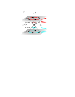
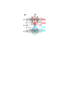
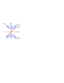
Figure 4: (A) 3D Landau level wavefunctions as spatially separated 2D helical Dirac modes localized along the $z$-axis. (B) 4D Landau level wavefunctions as spatially separated 3D Weyl modes localized along the $u$-axis. Note that 2D plane-wave modes with opposite helicities and the 3D ones with opposite chiralities are located at opposite sides of $z=0$ and $u=0$ planes, respectively. C) The central positions $u_{0}(m,k_{z},\nu)$ of the 4d Landau levels in the presence of the magnetic field $\vec{B}=B\hat{z}$. The branch of $m=0$ runs across the entire $u$-axis, which gives rise to quantized charge transport along $u$-axis in the presence of $\vec{E}\parallel\vec{B}$ as indicated in Eq. 49. From Ref. Li et al. (2013).

VII.3 Spatially separated 3D Weyl modes –4D Landau level

Again we can easily generalize the above procedure to any dimensions. For example, in four dimensions, we need to use the 3d helicity operator $\hat{\Sigma}_{3d}=\hat{P}_{3d}\cdot\vec{\sigma}$, whose eigenstates are denoted as $\chi_{\Sigma}$ with the eigenvalues $\Sigma=\pm 1$. Then the 4D Landau level Hamiltonian is defined as Li et al. (2013)

$$H^{4d,\mp}_{LL} = \frac{P_{u}^{2}+\vec{P}_{3d}^{2}}{2M}+\frac{1}{2}M\omega^{2}u^{2}\mp\omega u\vec{P}_{3d}\cdot\vec{\sigma}$$ (109)

$$= \frac{P_{u}^{2}}{2M}+\frac{1}{2}M\omega_{so}^{2}(u\mp\frac{1}{\hbar}l_{so}^{2}\vec{P}_{3d}\cdot\vec{\sigma})^{2},\ \ \,$$

where $u$ and $P_{u}$ are the coordinate and momentum in the 4th dimension, respectively, and $\vec{P}_{3d}$ is defined in the $xyz$-space. Inside each Landau level, the spectra are flat with respect to $\vec{k}_{3d}$ and $\Sigma$. Similarly to the 3D case, the 4D LL spectra and wavefunctions are solved by reducing Eq. 109 into a set of 1D harmonic oscillators along the $u$-axis as

$$\Psi_{n,\vec{k}_{3d},\Sigma}(\vec{r},u)=e^{i\vec{k}_{3d}\cdot\vec{r}}\phi_{n}[u-u_{0}(k_{3d},\Sigma)]\otimes\chi_{\Sigma}(\vec{k}_{3d}).$$ (110)

The central positions $u_{0}(k_{3d},\Sigma)=\Sigma l_{so}^{2}k_{3d}$. This realizes the spatial separation of the 3D Weyl fermion modes with the opposite chiralities as shown in Fig. 4 (B). With an open boundary imposed along the $u$-direction, the 3D chiral Weyl fermion modes appear on the boundary

$$H_{bd}=\pm v_{f}(\vec{k}_{3D}\cdot\vec{\sigma})-\mu.$$ (111)

VII.4 Phase space picture of high-dimensional Landau levels

For the 2D case described by Eq. 103, the $xy$-plane is equivalent to the 2D phase space of a 1D system $(x;k_{x})$ after the lowest Landau level projection. The discrete step of $k_{x}$ is $\Delta k_{x}=2\pi/L_{x}$, and the momentum cutoff of the bulk state is determined by $L_{y}$ as $k_{bk}=L_{y}/(2l_{B}^{2})$. Since $|k_{x}|<k_{bk}$, the number of states $N_{2D,LL}$ scales with $L_{x}L_{y}$ as the usual 2D systems, but the crucial difference is that enlarging $L_{y}$ does not change $\Delta k_{x}$ but instead increases $k_{bk}$.

Similarly, the 3D Landau level states (Eq. LABEL:eq:3D_Landau) can be viewed as states in the 4D phase space ($xy;k_{x}k_{y}$). The $z$-axis plays the double role of $k_{x}$ and $k_{y}$. After the lowest Landau level projection, $z$ is equivalent to $z=l_{so}^{2}(p_{x}\sigma_{y}-p_{y}\sigma_{x})/\hbar$, and thus

$$[x,z]_{LLL}=il_{so}^{2}\sigma_{y},\ \ \,[y,z]_{LLL}=-il_{so}^{2}\sigma_{x},$$

$$[x,y]_{LLL}=0.$$ (112)

The momentum cutoff of the bulk state is determined as $(k_{x}^{2}+k^{2}_{y})^{\frac{1}{2}}<k_{bk}=\hbar L_{z}/(2l_{so}^{2})$, thus the total number of states $N$ scales as $L_{x}L_{y}L_{z}^{2}$. As a result, the 3D local density of states linearly diverges as $\rho_{3D}(z)\propto|z|/l_{so}^{4}$ as $|z|\rightarrow\infty$. Similar divergence also occurs in the symmetric-like gauge as $\rho_{3D}(r)\propto r/l_{so}^{4}$. Now this seeming pathological result can be understood as the consequence of squeezing states of 4D phase space $(xy;k_{x}k_{y})$ into the 3D real space $(xyz)$. In other words, the correct thermodynamic limit should be taken according to the volume of 4D phase space. This reasoning is easily extended to the 4D LL systems (Eq.109), which can be understood as a 6D phase space of $(xyz;k_{x}k_{y}k_{z})$.

VII.5 Charge pumping and the 4D quantum Hall effects

The above 4D Landau level states presented in Sect. VII.3 exhibit non-linear electromagnetic response Zhang and Hu (2001); Qi et al. (2008); Werner (2012); Fröhlich and Pedrini (2000) as the 4D quantum Hall effect. We apply the electromagnetic fields as

$$\vec{E}=E\hat{z},\ \ \,\vec{B}=B\hat{z},$$ (113)

to the 4D Landau level Hamiltonian Eq. 109 by minimally coupling fermions to the $U(1)$ vector potential,

$$A_{em,x}=0,\ \ \,A_{em,y}=Bx,\ \ \,A_{em,z}=-cEt.$$ (114)

The $\vec{B}$-field further quantizes the chiral plane-wave modes inside the $n$-th 4D spin-orbit Landau level states into a series of 2D magnetic Landau level states in the $xy$-plane as labeled by the magnetic Landau level index $m$. For the case of $m=0$, the eigen-wavefunctions are spin polarized as

$$\Psi_{n,m=0}(k_{y},k_{z}) = e^{ik_{y}y+ik_{z}z}\phi_{n}(u-u_{0}(k_{z},m=0))$$ (115)

$$\times \varphi_{m=0}(x-x_{0}(k_{y}))\otimes|\uparrow\rangle,$$

where $\phi_{n}$ is the $n$-th order harmonic oscillator wavefunction with the spin-orbit length scale $l_{so}$, and $\varphi_{0}$ is the zeroth order harmonic oscillator wavefunction with the magnetic length scale $l_{B}$. The central positions of the $u$-directional and $x$-directional oscillators are

$$x_{0}(k_{y})=l_{B}^{2}k_{y},\ \ \,u_{0}(k_{z},m=0)=l_{so}^{2}k_{z},$$ (116)

respectively. The key point is that $u_{0}(k_{z},m=0)$ runs across the entire $u$-axis. In contrast, wavefunctions $\Psi_{n,m}$ with $m\geq 1$ also exhibit harmonic oscillator wavefunctions along the $u$-axis. However, their central positions at $m\geq 1$ are,

$$u_{0}(k_{z})=\pm l_{so}^{2}\sqrt{k_{z}^{2}+\frac{2m}{l_{B}^{2}}},$$ (117)

which only lie in half of the $u$-axis as shown in Fig. 4 (C).

Since $k_{z}$ increases with time in the presence of $E_{z}$, $u_{0}(m,k_{z}(t))$ moves along the $u$-axis. Only the $m=0$ branch of the magnetic Landau level states contribute to the charge pumping since their centers go across the entire $u$-axis, which results in an electric current along the $u$-direction. Since $k_{z}(t)=k_{z}(0)-\frac{eE}{\hbar}t$, during the time interval $\Delta t$, the number of electrons passing the cross-section at a fixed $u$ is

$$\Delta N=\frac{L_{x}L_{y}}{2\pi l_{B}^{2}}\frac{eE_{z}\Delta t}{2\pi\hbar/L_{z}}=\frac{e^{2}}{4\pi^{2}\hbar^{2}c}\vec{E}\cdot\vec{B}V\Delta t,$$ (118)

where $V$ is the 3D cross-volume. Then the current density is calculated as

$$j_{u}=n_{occ}\frac{e\Delta N}{V\Delta t}=n_{occ}\alpha\frac{e}{4\pi^{2}\hbar}\vec{E}\cdot\vec{B},$$ (119)

where $\alpha$ is the fine-structure constant, and $n_{occ}$ is the occupation number of the 4D spin-orbit Landau levels.

Eq. 119 is in agreement with results from the effective field theory Qi et al. (2008) as the 4D generalization of the quantum Hall effect. If we impose the open boundary condition perpendicular to the $u$-direction, the above charge pump process corresponds to the chiral anomalies of Weyl fermions with opposite chiralities on two opposite 3D boundaries, respectively. Since they are spatially separated, the chiral current corresponds to the electric current along the $u$-direction.

VIII Conclusions and outlooks

I have reviewed a general framework to construct Landau levels in high dimensions based on harmonic oscillator wavefunctions. By imposing spin-orbit coupling, their spectra are reorganized to exhibit flat dispersions. In particular, the lowest Landau level wavefunctions in 3D and 4D in the quaternion representation satisfy the Cauchy-Riemann-Fueter condition, which is the generalization of complex analyticity to high dimensions. The boundary excitations are the 2D helical Dirac surface modes, or, the 3D chiral Weyl modes. There is a beautiful bulk-boundary correspondence that the Cauchy-Riemann-Fueter condition and the helical Dirac (chiral Weyl) equation are the Euclidean and Minkowski representations of the same analyticity condition, respectively. By dimensional reductions, we constructed a class of Landau levels in 2D and 3D which are time-reversal invariant but parity breaking. The Landau level problem for Dirac fermions is a square-root problem of the non-relativistic one, corresponding to complex quaternions. The zeroth Landau level states are a flat band of half-fermion Jackiw-Rebbi zero modes. It is at the interface between condensed matter and high energy physics, related to a new type of anomaly. Unlike parity anomaly and chiral anomaly studied in field theory in which Dirac fermions are coupled to gauge fields through the minimal coupling, here Dirac fermions are coupled to background fields in a non-minimal way.

I speculate that high-dimensional Landau levels could provide a platform for exploring interacting topological states in high dimensions - due to the band flatness, and also the quaternionic analyticity of lowest Landau level wavefunctions. It would stimulate the developments of various theoretical and numerical methods. This would be an important direction in both condensed matter physics and mathematical physics for studying high dimensional topological states for both non-relativistic and relativistic fermions. This research also provides interesting applications of quaternion analysis in theoretical physics.

IX Acknowledgments

I thank Yi Li for collaborations on this set of works on high-dimensional topological states and for bringing in interesting concepts including the quaternionic analyticity. I also thank J. E. Hirsch for stimulating discussions, and S. C. Zhang, T. L. Ho, E. H. Fradkin, S. Das Sarma, F. D. M. Haldane, and C. N. Yang for their warm encouragements and appreciations.

Appendix A Brief review on Clifford algebra

In this part, we review how to construct anti-commutative $\Gamma$-matrices. The familiar group is just the $2\times 2$ Pauli matrices, i.e., rank-1. The rank-$k$ $\Gamma$-matrices can be defined recursively based on the rank-$(k-1)$ ones. At each level, there are $2k+1$ anti-commutative matrices, and their dimensions are $2^{k}\times 2^{k}$. In this article, we use the following representation,

$$\Gamma^{(k)}_{i} = \left[\begin{array}[]{cc}0&\Gamma_{a}^{(k-1)}\\ \Gamma_{a}^{(k-1)}&0\end{array}\right],\ \ \,\Gamma^{(k)}_{2k}=\left[\begin{array}[]{cc}0&-iI\\ iI&0\end{array}\right],$$ (124)

$$\Gamma^{(k)}_{2k+1} = \left[\begin{array}[]{cc}I&0\\ 0&-I\end{array}\right],$$ (127)

where $i=1,...,2k-1$.

In $D=2k+1$-dimensional space, the $SO(2k+1)$ fundamental spinor is $2^{k}$-dimensional. The generators are constructed $S_{ij}=\frac{1}{2}\Gamma_{ij}^{(k)}$ where

$$\Gamma^{(k)}_{ij}=-\frac{i}{2}[\Gamma^{(k)}_{i},\Gamma_{j}^{(k)}].$$ (128)

In the $D=2k$-dimensional space, there are two irreducible fundamental spinor representations for the $SO(2k)$ group, both of which are with $2^{k-1}$-dimensional. Their generators are denoted as $S_{ij}$ and $S_{ij}^{\prime}$, respectively, which can be constructed based on both rank-$(k-1)$ $\Gamma_{i}^{(k-1)}$ and $\Gamma_{ij}^{(k-1)}$-matrices. For the first $2k-1$ dimensions, the generators share the same form as that of the $SO(2k-1)$ group,

$$S_{ij}=S^{\prime}_{ij}=\frac{1}{2}\Gamma_{ij}^{(k-1)},\ \ \,(1\leq i<j\leq 2k-1).$$ (129)

Other generators $S_{i,2k}$ and $S_{i,2k}^{\prime}$ differ by a sign – they are represented by the $\Gamma^{(k-1)}_{i}$ matrices,

$$S_{i,2k}=S^{\prime}_{i,2k}=\pm\frac{1}{2}\Gamma_{i}^{(k-1)},\ \ \,(1\leq i\leq 2k-1).$$ (130)

References

- Sudbery (1979) A. Sudbery, Math. Proc. Cambridge Philos. Soc 85, 199 (1979).
- Adler (1995) S. L. Adler, Quaternionic quantum mechanics and quantum fields, vol. 88 (Oxford University Press, USA, 1995).
- Finkelstein (1962) D. Finkelstein, Journal of Mathematical Physics 3, 207 (1962).
- Yang (2005) C. N. Yang, Selected Papers (1945-1980) with Commentary (World Scientific, 2005).
- Bernevig and Zhang (2006) B. A. Bernevig and S. C. Zhang, Phys. Rev. Lett. 96, 106802 (2006), ISSN 1079-7114.
- Kane and Mele (2005a) C. L. Kane and E. J. Mele, Phys. Rev. Lett. 95, 146802 (2005a), ISSN 1079-7114.
- Kane and Mele (2005b) C. L. Kane and E. J. Mele, Phys. Rev. Lett. 95, 226801 (2005b), ISSN 1079-7114.
- Fu and Kane (2007) L. Fu and C. L. Kane, Phys. Rev. B 76, 045302 (2007), ISSN 1550-235X.
- Fu et al. (2007) L. Fu, C. L. Kane, and E. J. Mele, Phys. Rev. Lett. 98, 106803 (2007), ISSN 1079-7114.
- Moore and Balents (2007) J. E. Moore and L. Balents, Phys. Rev. B 75, 121306 (2007), ISSN 1550-235X.
- Bernevig et al. (2006) B. A. Bernevig, T. L. Hughes, and S. C. Zhang, Science 314, 1757 (2006).
- Wu et al. (2006) C. Wu, B. Bernevig, and S.-C. Zhang, Phys. Rev. Lett. 96, 106401 (2006), ISSN 1079-7114.
- Qi et al. (2008) X. L. Qi, T. L. Hughes, and S. C. Zhang, Phys. Rev. B 78, 195424 (2008), ISSN 1550-235X.
- Roy (2009) R. Roy, Phys. Rev. B 79, 195322 (2009), ISSN 1550-235X.
- Roy (2010) R. Roy, New J. Phys. 12, 065009 (2010).
- Thouless et al. (1982) D. J. Thouless, M. Kohmoto, M. P. Nightingale, and M. den Nijs, Phys. Rev. Lett. 49, 405 (1982), ISSN 1079-7114.
- Haldane (1988) F. D. M. Haldane, Phys. Rev. Lett. 61, 2015 (1988), ISSN 1079-7114.
- Kitaev (2009) A. Kitaev, in American Institute of Physics Conference Series (2009), vol. 1134, pp. 22–30.
- Schnyder et al. (2008) A. Schnyder, S. Ryu, A. Furusaki, and A. Ludwig, Phys. Rev. B 78, 195125 (2008), ISSN 1550-235X.
- Klitzing et al. (1980) K. Klitzing, G. Dorda, and M. Pepper, Phys. Rev. Lett. 45, 494 (1980), ISSN 1079-7114.
- Tsui et al. (1982) D. C. Tsui, H. L. Stormer, and A. C. Gossard, Phys. Rev. Lett. 48, 1559 (1982), URL http://link.aps.org/doi/10.1103/PhysRevLett.48.1559.
- Girvin (1999) S. Girvin, Aspects topologiques de la physique en basse dimension. Topological aspects of low dimensional systems pp. 53–175 (1999).
- Laughlin (1983) R. Laughlin, Phys. Rev. Lett. 50, 1395 (1983), ISSN 1079-7114.
- Zhang and Hu (2001) S. C. Zhang and J. P. Hu, Science 294, 823 (2001).
- Haldane (1983) F. D. M. Haldane, Phys. Rev. Lett. 51, 605 (1983).
- Li et al. (2012a) Y. Li, X. Zhou, and C. Wu, Phys. Rev. B 85, 125122 (2012a).
- Li and Wu (2013) Y. Li and C. Wu, Phys. Rev. Lett. 110, 216802 (2013), URL https://link.aps.org/doi/10.1103/PhysRevLett.110.216802.
- Li et al. (2012b) Y. Li, K. Intriligator, Y. Yu, and C. Wu, Phys. Rev. B 85, 085132 (2012b).
- Jackiw and Rebbi (1976) R. Jackiw and C. Rebbi, Phys. Rev. D 13, 3398 (1976), URL http://link.aps.org/doi/10.1103/PhysRevD.13.3398.
- Li et al. (2013) Y. Li, S.-C. Zhang, and C. Wu, Phys. Rev. Lett. 111, 186803 (2013), URL https://link.aps.org/doi/10.1103/PhysRevLett.111.186803.
- Frenkel and Libine (2008) I. Frenkel and M. Libine, Advances in Mathematics 218, 1806 (2008), ISSN 0001-8708, URL http://www.sciencedirect.com/science/article/pii/S0001870808000935.
- Balatsky (1992) A. V. Balatsky, arXiv:cond-mat/9205006 (1992).
- Semenoff (1984) G. W. Semenoff, Phys. Rev. Lett. 53, 2449 (1984).
- Heeger et al. (1988) A. J. Heeger, S. Kivelson, J. R. Schrieffer, and W. P. Su, Rev. Mod. Phys. 60, 781 (1988), URL http://link.aps.org/doi/10.1103/RevModPhys.60.781.
- Redlich (1984a) A. N. Redlich, Phys. Rev. Lett. 52, 18 (1984a), URL http://link.aps.org/doi/10.1103/PhysRevLett.52.18.
- Redlich (1984b) A. N. Redlich, Phys. Rev. D 29, 2366 (1984b), URL http://link.aps.org/doi/10.1103/PhysRevD.29.2366.
- Niemi and Semenoff (1986) A. J. Niemi and G. W. Semenoff, Physics Reports 135, 99 (1986).
- Streda (1982) P. Streda, Journal of Physics C: Solid State Physics 15, L1299 (1982), URL http://stacks.iop.org/0022-3719/15/i=36/a=006.
- Bagchi (2001) B. K. Bagchi, Supersymmetry in quantum and classical mechanics (Chapman & Hall/CRC, 2001), ISBN 1584881976.
- Lee and Kane (1990) D. H. Lee and C. L. Kane, Phys. Rev. Lett. 64, 1313 (1990), URL http://link.aps.org/doi/10.1103/PhysRevLett.64.1313.
- Sondhi et al. (1993) S. L. Sondhi, A. Karlhede, S. A. Kivelson, and E. H. Rezayi, Phys. Rev. B 47, 16419 (1993).
- Fertig et al. (1994) H. A. Fertig, L. Brey, R. Côté, and A. H. MacDonald, Phys. Rev. B 50, 11018 (1994), URL http://link.aps.org/doi/10.1103/PhysRevB.50.11018.
- Read and Sachdev (1995) N. Read and S. Sachdev, Phys. Rev. Lett. 75, 3509 (1995), URL http://link.aps.org/doi/10.1103/PhysRevLett.75.3509.
- Haldane and Rezayi (1985) F. D. M. Haldane and E. H. Rezayi, Phys. Rev. Lett. 54, 237 (1985), URL http://link.aps.org/doi/10.1103/PhysRevLett.54.237.
- Prange and Girvin (1990) R. E. Prange and S. M. Girvin, eds., The Quantum Hall Effect (Springer-Verlag, New York, 1990), 2nd ed.
- Haldane (2011) D. Haldane, Phys. Rev. Lett. 107, 116801 (2011).
- Can et al. (2014) T. Can, M. Laskin, and P. Wiegmann, Phys. Rev. Lett. 113, 046803 (2014), eprint 1402.1531.
- Klevtsov et al. (2017) S. Klevtsov, X. Ma, G. Marinescu, and P. Wiegmann, Communications in Mathematical Physics 349, 819 (2017), eprint 1510.06720.
- Wu et al. (2011) C. J. Wu, I. Mondragon-Shem, and Z. Xiang-Fa, Chinese Physics Letters 28, 097102 (2011), URL http://stacks.iop.org/0256-307X/28/i=9/a=097102.
- Li et al. (2016) Y. Li, X. Zhou, and C. Wu, Phys. Rev. A 93, 033628 (2016), URL https://link.aps.org/doi/10.1103/PhysRevA.93.033628.
- Wu and Mondragon-Shem (2008) C. Wu and I. Mondragon-Shem, arXiv:0809.3532v1 (2008).
- Zhou et al. (2013) X. Zhou, Y. Li, Z. Cai, and C. Wu, Journal of Physics B Atomic Molecular Physics 46, 134001 (2013), eprint 1301.5403.
- Hu et al. (2012) H. Hu, B. Ramachandhran, H. Pu, and X. J. Liu, Phys. Rev. Lett. 108, 010402 (2012), URL http://link.aps.org/doi/10.1103/PhysRevLett.108.010402.
- Sinha et al. (2011) S. Sinha, R. Nath, and L. Santos, Phys. Rev. Lett. 107, 270401 (2011), URL http://link.aps.org/doi/10.1103/PhysRevLett.107.270401.
- Ghosh et al. (2011) S. K. Ghosh, J. P. Vyasanakere, and V. B. Shenoy, Phys. Rev. A 84, 053629 (2011), URL http://link.aps.org/doi/10.1103/PhysRevA.84.053629.
- Wang et al. (2010) Z. Wang, X.-L. Qi, and S.-C. Zhang, New J. Phys. 12, 065007 (2010).
- Ho and Zhang (2011) T.-L. Ho and S. Zhang, Phys. Rev. Lett. 107, 150403 (2011), URL http://link.aps.org/doi/10.1103/PhysRevLett.107.150403.
- Xiao et al. (2010) D. Xiao, M. Chang, and Q. Niu, Rev. Mod. Phys. 82, 1959 (2010), ISSN 0034-6861.
- Callan and Harvey (1985) C. G. Callan and J. A. Harvey, Nuclear Physics B 250, 427 (1985), ISSN 0550-3213, URL http://www.sciencedirect.com/science/article/pii/0550321385904894.
- Lee and Leinaas (2004) D. H. Lee and J. M. Leinaas, Phys. Rev. Lett. 92, 096401 (2004), URL http://link.aps.org/doi/10.1103/PhysRevLett.92.096401.
- Werner (2012) P. Werner, arXiv:1207.4954 (2012).
- Fröhlich and Pedrini (2000) J. Fröhlich and B. Pedrini, arXiv:hep-th/0002195 (2000).