Spectral Cauchy-characteristic extraction of the gravitational wave news function

Abstract

We present an improved spectral algorithm for Cauchy-characteristic extraction and characteristic evolution of gravitational waves in numerical relativity. The new algorithms improve spectral convergence both at the poles of the spherical-polar grid and at future null infinity, as well as increase the temporal resolution of the code. The key to the success of these algorithms is a new set of high-accuracy tests, which we present here. We demonstrate the accuracy of the code and compare with the existing PittNull implementation.

I Introduction

The discovery of GW150914 Abbott et al. (2016a) heralded the beginning of gravitational wave astronomy. In the subsequent years that detection has been followed up by a number of other signals observed from binary black hole (BBH) mergers Abbott et al. (2016b, 2017a, 2017b, 2017c), as well as from the merger of a binary neutron star (BNS) system Abbott et al. (2017d). As the aLIGO Aasi et al. (2015) and Virgo Acernese et al. (2015) detectors push to ever greater sensitivities, the number of expected observations will continue to grow.

Extracting the signals from the noise involves matching the incoming data against a template bank of theoretically expected waveforms generated across possible binary configurations. The efficacy of extracting the configuration parameters (for instance, masses and spins of the binary components) from a given signal depends on the fidelity of the computed waveforms comprising the template bank; this is because errors in the template bank will bias the estimated parameters. The only ab initio method of generating accurate theoretical waveforms for merging BBH systems is via numerical relativity: the numerical solution of the full Einstein equations on a computer. Other methods of generating theoretical BBH waveforms, such as effective one-body solutions Bohé et al. (2017) and phenomenological models Husa et al. (2016); Khan et al. (2016), are calibrated to numerical relativity.

One limitation of numerical relativity simulations is that they all rely on a Cauchy approach in which the spacetime is decomposed into a foliation of spacelike slices, and the solution marches from one slice to the next. Such an approach can compute the solution to Einstein’s equations only in a region of spacetime with finite spatial and temporal extents bounded around the compact objects, whereas the gravitational radiation is defined at future null infinity $\mathscr{I}^{+}$. While some work has gone into hyperboloidal compactification methods for simulating the propagation of gravitational waves to $\mathscr{I}^{+}$ Husa et al. (2006); Zenginoglu and Husa (2006); Zenginoğlu (2008), these methods have never been fully implemented in the nonlinear regime. Without them, extracting the waveform signal from the simulations with these finite extents requires additional work.

The most common method of extracting the gravitational radiation from a numerical relativity simulation is to compute quantities such as the Newman-Penrose scalar $\Psi_{4}$ Newman and Penrose (1962) or the Regge-Wheeler and Zerilli scalars Sarbach and Tiglio (2001) at some large but finite distance from the near zone (perhaps 100-1000$M$, where $M$ is the total mass of the system), typically on coordinate spheres of constant surface area coordinate coordinate $r$. Because these quantities or the methods of computing them include finite-radius effects, these quantities are computed on a series of shells at different radii $r$, fit to a polynomial in $1/r$, and then extrapolated to infinity by reading off the $1/r$ coefficient of the polynomial Boyle and Mroué (2009). As the extraction surfaces are shells of constant coordinate radii, the choice of gauge implemented in the simulation can contaminate the resulting waveforms. Furthermore, if the shells are too close to the orbiting binary, the extrapolation procedure might not remove all of the near-zone effects.

An alternative method for computing gravitational radiation in numerical relativity is to solve the full Einstein equations in a domain that extends all the way to $\mathscr{I}^{+}$, where gravitational waves can be measured. This can be done by rewriting Einstein’s equations using a characteristic formalism Bondi et al. (1962); Sachs (1962a); Penrose (1963), in which the equations are solved on outgoing null surfaces that extend to $\mathscr{I}^{+}$. This formalism chooses coordinates that correspond to distinct outward propagating null rays, so it fails in the dynamical, strong field regime at any location where outgoing null rays intersect (i.e., caustics). Because of this, characteristic evolution is unable to evolve the near-field region of a merging binary system, so it cannot accomplish a BBH simulation on its own. However, it is possible to combine an interior numerical relativity code that solves the equations on Cauchy slices with an exterior characteristic code that solves them on null slices; the determination of characteristic quantities from Cauchy data is known as Cauchy-characteristic extraction (CCE) (see Fig. 1), and the subsequent numerical evolution of those quantities is known as characteristic evolution.

Specifically, CCE uses the metric and its derivatives computed from a Cauchy evolution (red region in Fig. 1) and evaluated on a worldtube $\Gamma$ (thick red line) that lies on or inside the boundary of the Cauchy region. These quantities on the worldtube are then used as inner boundary data for a characteristic evolution (blue region) based on outgoing null slices (blue curves). Because the combined CCE system uses the full Einstein equations for both the Cauchy and characteristic evolutions, it produces the correct solution at $\mathscr{I}^{+}$, with the characteristic evolution properly resolving near-zone effects. The gravitational radiation is computed according to a particular inertial observer at $\mathscr{I}^{+}$ (green curve). This observer is related to any other inertial observer by a single Bondi-Metzner-Sachs (BMS) transformation Sachs (1962a) (the group of Lorentz boosts, rotations, and supertranslations Sachs (1962b)), so up to this BMS transformation the waveform is independent of the gauge chosen by the Cauchy evolution.

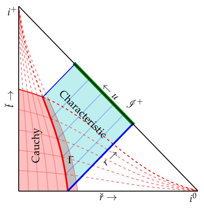
Figure 1: Penrose diagram showing a typical CCE setup. The metric is evolved using 3+1 methods in the Cauchy region (shaded red) and with null methods in the characteristic region (shaded blue). The Cauchy and characteristic regions overlap. Curves of constant $\breve{t}$ or $\breve{r}$, the Cauchy coordinates, are shown in red, and are shown as dashed curves outside the Cauchy region, where they extend to spatial infinity $i^{0}$ or future temporal infinity $i^{+}$. Null curves of constant $u$ are shown in blue. Given data on a worldtube $\Gamma$ (thick red curve) and on an initial null slice (thick blue curve), the characteristic evolution computes the full metric in the characteristic region. In Sec. III we describe the interface from Cauchy to Bondi coordinates on $\Gamma$. In Sec. IV we describe the characteristic evolution. In Sec. V we discuss computing the news function at $\mathscr{I}^{+}$ (thick green curve) and transforming it to coordinates corresponding to a free-falling observer.

The first code to implement CCE and characteristic evolution was the PittNull code Bishop et al. (1996, 1997, 1998). Since its initial implementation there have been a number of improvements made, and the current iteration of that code utilizes stereographic angular coordinate patches, finite differencing, and a null parallelogram scheme with fixed time steps for integrating in the null and time directions. Overall the code is second-order convergent with resolution Reisswig et al. (2007); Babiuc et al. (2011) (although a fourth-order implementation also exists, see Reisswig et al. (2013)). Compared to waveforms computed from a Cauchy code by evaluating $\Psi_{4}$ at finite radii and extrapolating to $r\to\infty$ as described above, waveforms extracted via CCE using PittNull were shown to better remove gauge effects and to better resolve the $m=0$ memory modes Reisswig et al. (2010); Pollney and Reisswig (2011); Taylor et al. (2013).

Currently, PittNull requires thousands of CPU hours to compute a waveform at $\mathscr{I}^{+}$ given worldtube output from a typical Cauchy BBH simulation at multiple resolutions Handmer and Szilágyi (2015). While that cost is smaller than the computational expense of the Cauchy simulation, it is still unwieldy, and is likely one reason that most Cauchy numerical-relativity codes do not use CCE and characteristic evolution despite the availability of PittNull. Because the metric in the characteristic region is smooth, the computational cost of characteristic evolution should be greatly reduced by using spectral methods instead of finite differencing. Such a spectral implementation of characteristic evolution has been introduced in the SpEC framework Handmer and Szilágyi (2015); Handmer et al. (2015, 2016). Their tests showed improved speed and accuracy over the finite-difference implementation of PittNull Handmer and Szilágyi (2015); Handmer et al. (2015).

Our work here describes improvements in accuracy, efficiency, and robustness to the code described in Handmer and Szilágyi (2015); Handmer et al. (2015, 2016). In particular, we discuss an improved handling of the integration along the null slices, we clarify issues related to the particular choice of coordinates along the null slice, and we implement better handling of the inertial coordinates at $\mathscr{I}^{+}$. We demonstrate through a series of analytic tests that our version of CCE and characteristic evolution can compute waveforms with much lower computational cost than PittNull. An earlier version of our implementation has been used to probe the near-field region of a binary black hole ringdown Bhagwat et al. (2017).

We start with a brief summary of the Bondi metric and the null formulation of the Einstein equations in Sec. II. A detailed explanation for how CCE and characteristic evolution works can be broken up into three distinct parts: the inner boundary formalism, the volume characteristic evolution, and the $\mathscr{I}^{+}$ extraction, which we describe in subsequent sections. Section III describes the means by which the metric known on a worldtube is converted into Bondi form to serve as the inner boundary values for the characteristic evolution system. Section IV discusses the process of evolving Einstein’s equations from the inner boundary to $\mathscr{I}^{+}$. Section V explains how to take the metric computed on $\mathscr{I}^{+}$ and extract the Bondi news function in the frame of an inertial observer at $\mathscr{I}^{+}$. In Sec. VI, we describe code tests and performance.

Throughout this paper, indices with Greek letters ($\mu,\nu,\ldots$) correspond to spacetime coordinates, lowercase Roman letters ($i,j,\ldots$) to spatial coordinates, and capitalized Roman letters ($A,B,\ldots$) to angular coordinates, and we choose a system of geometrized units ($c=G=1$). For convenience, we have included a definitions key in Appendix C.

II Summary of characteristic formulation

In the characteristic region (see Fig. 1), we adopt a coordinate system $x^{\mu}=(u,r,x^{A})$, where $u$ is the coordinate labeling the outgoing null cones, $r$ is an areal radial coordinate, and $x^{A}$ are the angular coordinates. Note that a curve of constant $(u,x^{A})$ is an outgoing null ray parametrized by $r$; for this reason we sometimes call $r$ a “radinull” coordinate. The metric can then be expressed in the Bondi-Sachs form Bondi et al. (1962); Sachs (1962a),

$$ds^{2}= -\left(e^{2\beta}\left(1+rW\right)-r^{2}h_{AB}U^{A}U^{B}\right)du^{2}$$

$$- 2e^{2\beta}dudr-2r^{2}h_{AB}U^{B}dudx^{A}$$

$$+ r^{2}h_{AB}dx^{A}dx^{B},$$ (1)

where $W$ corresponds to the mass aspect, $U^{A}$ to the shift, $\beta$ to the lapse, and $h_{AB}$ to the spherical 2-metric. The quantity $h_{AB}$ has the same determinant as the unit sphere metric $q_{AB}$, $|h_{AB}|=|q_{AB}|$. Note that the metric Eq. (1) is not constrained to be asymptotically flat, as required by Bondi-Sachs coordinates. Instead, we impose the weaker constraint that all metric components of Eq. (1) are asymptotically finite at $\mathcal{I}^{+}$. To emphasize this subtle difference with Bondi-Sachs coordinates, we refer to the spacetime metric as having the “Bondi-Sachs form” rather than being expressed in Bondi-Sachs coordinates. An additional intermediate quantity, $Q_{A}$, is defined to reduce the evolution equations to a series of first order partial differential equations (PDEs),

$$Q_{A}=r^{2}e^{-2\beta}h_{AB}U^{B}_{,r}.$$ (2)

Instead of expressing the metric in terms of tensorial objects, we employ a complex dyad so that the metric components can be computed as spin-weighted scalars, and each of these scalars can be expanded in terms of spin-weighted spherical harmonics (SWSHes) of the appropriate spin weight; see Appendix A for details about SWSHes. The dyad $q^{A}$ has the following properties:

$$q^{A}q_{A}= 0,$$ (3)

$$q^{A}\bar{q}_{A}= 2.$$ (4)

If we define $q_{AB}$ and $q^{AB}$ such that

$$q_{AB}= \frac{1}{2}(q_{A}\bar{q}_{B}+\bar{q}_{A}q_{B}),$$ (5)

$$q^{AC}q_{CB}= \delta^{A}_{B},$$ (6)

then

$$q^{A}= q^{AB}q_{B}.$$ (7)

We express the metric coefficients and the quantity $Q_{A}$ in terms of spin-weighted scalars $J$, $K$, $U$, and $Q$, defined by

$$J= \frac{1}{2}h_{AB}q^{A}q^{B},$$ (8)

$$K= \frac{1}{2}h_{AB}q^{A}\bar{q}^{B},$$ (9)

$$U= q_{A}U^{A},$$ (10)

$$Q= Q_{A}q^{A}.$$ (11)

The determinant condition on $h_{AB}$ defines a relationship between $J$ and $K$ as

$$K=\sqrt{1+J\bar{J}}.$$ (12)

We introduce one more intermediate variable $H$, the time derivative of $J$ along slices of constant $r$,

$$H=J_{,u|x^{A},r=\text{const}}$$ (13)

The quantities $J,\beta,$ and $Q$ are all dimensionless while $U,W,$ and $H$ have units of $1/R$ (identically, units of $1/u$ in the case of $H$).

Evaluating the components of the Einstein equation $G_{\mu\nu}=0$ provides a system of equations for the quantities $\beta$, $Q$, $U$, $W$, and $H$:

$$\beta_{,r}= \mathcal{N}_{\beta},$$ (14)

$$(r^{2}Q)_{,r}= -r^{2}(\bar{\eth}J+\eth K)_{,r}+2r^{4}\eth(r^{-2}\beta)_{,r}$$

$$+ \mathcal{N}_{Q},$$ (15)

$$U_{,r}= r^{-2}e^{2\beta}Q+\mathcal{N}_{U},$$ (16)

$$(r^{2}W)_{,r}= \frac{1}{2}e^{2\beta}\mathcal{R}-1-e^{\beta}\eth\bar{\eth}e^{\beta}$$

$$+ \frac{1}{4}r^{-2}(r^{4}(\eth\bar{U}+\bar{\eth}U))_{,r}+\mathcal{N}_{W},$$ (17)

$$2(rH)_{,r}= ((1+rW)(rJ)_{,r})_{,r}-r^{-1}(r^{2}\eth U)_{,r}$$

$$+ 2r^{-1}e^{\beta}\eth^{2}e^{\beta}-(rW)_{,r}J+\mathcal{N}_{J},$$ (18)

where

$$\mathcal{R}= 2K-\eth\bar{\eth}K+\frac{1}{2}(\bar{\eth}^{2}J+\eth^{2}\bar{J})+\frac{1}{4K}(\bar{\eth}\bar{J}\eth J-\bar{\eth}J\eth\bar{J}),$$ (19)

and $\mathcal{N}_{\beta},\mathcal{N}_{W},\mathcal{N}_{Q},\mathcal{N}_{W},$ and $\mathcal{N}_{J}$ are the terms nonlinear in $J$ and its derivatives, according to Bishop et al. (1996). Appendix B provides the full expressions for these equations.

These equations correspond to different components of the Einstein equations, namely, $R_{rr}=0$ gives the equation for $\beta_{,r}$, $R_{rA}q^{A}=0$ gives the equation for $U_{,r}$, $R_{AB}h^{AB}$=0 gives the equation for $W_{,r}$, and $R_{AB}q^{A}q^{B}=0$ gives the equation for $H_{,r}$. These cover six of the ten independent components of Einstein’s equations. As Bishop et al. (1997) discusses in more detail, of the four remaining components of the Einstein equations, one of these is identically zero ($R^{r}_{r}=0$) while the other three ($R^{r}_{u}=0$ and $R^{r}_{A}q^{A}=0$) serve as constraint conditions for the evolution on each of the null slices.

However, computing these constraint conditions involve lengthy expressions that include the $u$-derivatives of evolution quantities other than $J_{,u}$. It is not straightforward to compute these derivatives to the same accuracy achieved by the rest of the code. We leave to future implementations the ability to accurately compute these constraints as a monitor of how well we obey the full Einstein equations during the evolution.

The equations are presented in a useful hierarchical order: the right-hand side of the $\beta$ equation involves only $J$ and its hypersurface derivatives, the right-hand side of the $Q$ equation involves only $J$ and $\beta$ and their hypersurface derivatives, and so on for the other equations. Therefore, given data for all quantities on the inner boundary as well as $J$ on an initial $u=$ const null slice, we can integrate the series of equations in Eqs. (14)-(18) on that slice from the inner boundary to $r=\infty$ to obtain $\beta,Q,U,W,$ and then $H$ in sequence on that slice. Then, given $H=J_{,u|r=\text{const}}$ on that slice, we can integrate forward in time to obtain $J$ on the next null slice.

III Inner Boundary Formalism

The coordinates used to evolve Einstein’s equations in the Cauchy region (red area of Fig. 1) are generally different from the coordinates discussed in Sec. II. The Cauchy coordinates are chosen to make the interior evolution proceed without encountering coordinate singularities; the procedure for choosing these coordinates is complicated and typically involves coordinates that are evolved along with the solution Pretorius (2005); Lindblom et al. (2006); Szilágyi et al. (2009); Scheel et al. (2009); Campanelli et al. (2006); Baker et al. (2006). Therefore, for CCE we must transform from arbitrary Cauchy coordinates to coordinates such that the spacetime metric takes the Bondi-Sachs form [Eq. (1)] at the worldtube.

Here, in the Cauchy region, for simplicity we assume Cartesian coordinates $(\breve{t},\breve{x}^{\breve{\i}})$ in which the worldtube hypersurface $\Gamma$ (which is chosen by the Cauchy code) is a surface of constant $\breve{r}$, where $\breve{r}=\sqrt{\breve{x}^{2}+\breve{y}^{2}+\breve{z}^{2}}$.

We also define angular coordinates $\breve{x}^{\breve{A}}=(\breve{\theta},\breve{\phi})$ in the usual way from the Cartesian coordinates $\breve{x}^{\breve{\i}}$.

The worldtube serves as the inner boundary of the characteristic domain (see Fig. 1). On this boundary, we assume that the interior Cauchy code provides the spatial 3-metric $g_{\breve{\i}\breve{\j}}$, the shift $\beta^{\breve{\i}}$, and the lapse $\breve{\alpha}$, along with the $\breve{r}$ and $\breve{t}$ derivatives of each of these quantities. Angular derivatives of these quantities are necessary as well; however, we can compute those numerically within the worldtube itself, so they need not be provided a priori.

Reference Bishop et al. (1998) describes how to take the data provided by the interior Cauchy code and covert it into Bondi form [Eq. (1)] to extract the inner boundary values of the evolution quantities ($J_{|\Gamma},\beta_{|\Gamma},\ldots$). This section is primarily a summary of their results; however, we use different notation than Ref. Bishop et al. (1998). Additionally, as noted above, the SpEC CCE treatment takes the inner boundary of the domain to be the worldtube provided by the Cauchy code, which is generally not a surface of constant $r$. The PittNull treatment, on the other hand, uses a surface of constant $r$ as the inner boundary of the domain, and performs a Taylor expansion in the affine radial coordinate in order to determine inner boundary data on this surface. Avoiding the Taylor expansion simplifies the boundary computation and may provide marginal precision improvements by avoiding a finite Taylor series truncation error.

III.1 Affine null coordinates

Our goal is to transform from the coordinates $(\breve{t},\breve{x}^{\breve{\i}})$ to coordinates such that the metric takes the Bondi-Sachs form (Eq. (1)). It is simplest to proceed in two steps: the first step, described in this subsection, is to construct coordinates foliated by outgoing null geodesics. The second step, described in Sec. III.2, will be to transform from these affine coordinates to Bondi coordinates.

We begin by constructing a choice null generator $\ell^{\breve{\mu}}$, which involves the unit outward spatial vector normal to the worldtube’s surface, $s^{\breve{\mu}}$, and the unit timelike vector normal to a slice of constant $\breve{t}$, $n^{\breve{\mu}}$:

$$s^{\breve{\mu}}= \left\{0,\frac{g^{\breve{\i}\breve{\j}}\breve{x}_{\breve{\j}}}{\sqrt{g^{\breve{\i}\breve{\j}}\breve{x}_{\breve{\i}}\breve{x}_{\breve{\j}}}}\right\},$$ (20)

$$n^{\breve{\mu}}= \frac{1}{\breve{\alpha}}\left\{1,-\beta^{\breve{\i}}\right\}.$$ (21)

Equation (20) depends on our simplifying assumption that the worldtube is spherical in Cauchy coordinates, and can be generalized. From these equations, the null generator is

$$\ell^{\breve{\mu}}= \frac{n^{\breve{\mu}}+s^{\breve{\mu}}}{\breve{\alpha}-g_{\breve{\i}\breve{\j}}\beta^{\breve{\i}}s^{\breve{\j}}}.$$ (22)

The time derivatives of these vectors are

$$s^{\breve{\mu}}_{,\breve{t}}= \left\{0,~{}(-g^{\breve{\i}\breve{\j}}+s^{\breve{\i}}s^{\breve{\j}}/2)s^{\breve{k}}g_{\breve{\j}\breve{k},\breve{t}}\right\},$$ (23)

$$n^{\breve{\mu}}_{,\breve{t}}= \frac{1}{\breve{\alpha}^{2}}\left\{-\breve{\alpha}_{,\breve{t}},~{}\breve{\alpha}_{,\breve{t}}\beta^{\breve{\i}}-\breve{\alpha}\beta^{\breve{\i}}_{,\breve{t}}\right\},$$ (24)

$$\ell^{\breve{\mu}}_{,\breve{t}}= \frac{n^{\breve{\mu}}_{,\breve{t}}+s^{\breve{\mu}}_{,\breve{t}}+\ell^{\breve{\mu}}\left(-\breve{\alpha}_{,\breve{t}}+g_{\breve{\i}\breve{\j},\breve{t}}\beta^{\breve{\i}}s^{\breve{\j}}+g_{\breve{\i}\breve{\j}}\beta^{\breve{\i}}_{,\breve{t}}s^{\breve{\j}}+g_{\breve{\i}\breve{\j}}\beta^{\breve{\i}}s^{\breve{\j}}_{,\breve{t}}\right)}{\breve{\alpha}-g_{\breve{\i}\breve{\j}}\beta^{\breve{\i}}s^{\breve{\j}}}.$$ (25)

We will now construct a null coordinate system based on outgoing null geodesics generated by $\ell^{\breve{\mu}}$. Let $\bar{\lambda}$ be an affine parameter along these geodesics such that the value of $\bar{\lambda}$ on the worldtube $\Gamma$ is $\bar{\lambda}_{|\Gamma}=0$. We also define a null coordinate $\bar{u}$ and angular coordinates $\bar{x}^{\bar{A}}=(\bar{\theta},\bar{\phi})$ that obey $\bar{u}=\breve{t}$ and $\bar{x}^{\bar{A}}=\breve{x}^{\breve{A}}$ on the worldtube, and are constant along the outgoing null geodesic generated by $\ell^{\breve{\mu}}$. Thus we have defined a new intermediate, affine coordinate system, $\bar{x}^{\bar{\mu}}=(\bar{u},\bar{\lambda},\bar{\theta},\bar{\phi})$, and we will express the metric $g_{\bar{\mu}\bar{\nu}}$ in these affine coordinates.

To do this, we will need to write down the coordinate transformation from $\breve{x}^{\breve{\mu}}$ to $\bar{x}^{\bar{\mu}}$ in a neighborhood of the worldtube, not just on the worldtube itself, because we need derivatives of this transformation. In particular, we will need derivatives with respect to $\bar{\lambda}$. The derivative of the metric components $g_{\breve{\mu}\breve{\nu}}$ along the null direction simply is

$$g_{\breve{\mu}\breve{\nu},\bar{\lambda}}= \ell^{\breve{\gamma}}g_{\breve{\mu}\breve{\nu},\breve{\gamma}}.$$ (26)

The evolution of the coordinates $\breve{x}^{\breve{\mu}}$ along null geodesics implies that in a neighborhood of the worldtube

$$\breve{x}^{\breve{\mu}}_{,\bar{\lambda}}=\ell^{\breve{\nu}}\partial_{\breve{\nu}}\breve{x}^{\breve{\mu}}=\ell^{\breve{\mu}}.$$ (27)

Given the new coordinates $\bar{x}^{\bar{\mu}}$, the metric components in these coordinates are

$$g_{\bar{\mu}\bar{\nu}}=\frac{\partial\breve{x}^{\breve{\alpha}}}{\partial\bar{x}^{\bar{\mu}}}\frac{\partial\breve{x}^{\breve{\beta}}}{\partial\bar{x}^{\bar{\nu}}}g_{\breve{\alpha}\breve{\beta}}.$$ (28)

On the worldtube,

$$\frac{\partial\breve{t}}{\partial\bar{x}^{\bar{A}}} =0$$

$$\frac{\partial\breve{x}^{\breve{i}}}{\partial\bar{x}^{\bar{A}}} =\frac{\partial\breve{x}^{\breve{i}}}{\partial\breve{x}^{\breve{A}}}$$

$$\frac{\partial\breve{t}}{\partial\bar{u}} =1,$$

$$\frac{\partial\breve{x}^{\breve{\i}}}{\partial\bar{u}} =0,$$ (29)

where the term $\partial\breve{x}^{\breve{\i}}/\partial\bar{x}^{\bar{A}}$ is the standard Cartesian to spherical Jacobian. The above values of the Jacobians hold only on the worldtube. In addition to the metric itself, we will also need first derivatives of the metric, including the derivative with respect to $\bar{\lambda}$. This requires the $\bar{\lambda}$ derivatives of the Jacobians evaluated on the worldtube, which we represent here as

$$\frac{\partial^{2}\breve{x}^{\breve{\mu}}}{\partial\bar{x}^{\bar{A}}\partial\bar{\lambda}}= \frac{\partial\ell^{\breve{\mu}}}{\partial\bar{x}^{\bar{A}}}=\ell^{\breve{\mu}}_{,\bar{A}},$$

$$\frac{\partial^{2}\breve{x}^{\breve{\mu}}}{\partial\bar{u}\partial\bar{\lambda}}= \frac{\partial\ell^{\breve{\mu}}}{\partial\bar{u}}=\ell^{\breve{\mu}}_{,\bar{u}},$$ (30)

where we have made use of Eq. (27).

We are now ready to write out the metric in these intermediate coordinates by taking the expression in Eq. (28) and taking the appropriate derivatives,

$$g_{\bar{u}\bar{\lambda}}= -1,$$

$$g_{\bar{\lambda}\bar{\lambda}}= g_{\bar{\lambda}\bar{A}}=0,$$

$$g_{\bar{u}\bar{u}}= g_{\breve{t}\breve{t}},$$

$$g_{\bar{u}\bar{A}}= \frac{\partial\breve{x}^{\breve{\i}}}{\partial\bar{x}^{\bar{A}}}g_{\breve{\i}\breve{t}},$$

$$g_{\bar{A}\bar{B}}= \frac{\partial\breve{x}^{\breve{\i}}}{\partial\bar{x}^{\bar{A}}}\frac{\partial\breve{x}^{\breve{\j}}}{\partial\bar{x}^{\bar{B}}}g_{\breve{\i}\breve{\j}},$$

$$g_{\bar{A}\bar{B},\bar{\lambda}}= \frac{\partial\breve{x}^{\breve{\i}}}{\partial\bar{x}^{\bar{A}}}\frac{\partial\breve{x}^{\breve{\j}}}{\partial\bar{x}^{\bar{B}}}g_{\breve{\i}\breve{\j},\bar{\lambda}}$$

$$+ \left(\ell^{\breve{\mu}}_{~{},\bar{A}}\frac{\partial\breve{x}^{\breve{\i}}}{\partial\bar{x}^{\bar{B}}}+\ell^{\breve{\mu}}_{~{},\bar{B}}\frac{\partial\breve{x}^{\breve{\i}}}{\partial\bar{x}^{\bar{A}}}\right)g_{\breve{\mu}\breve{\i}},$$

$$g_{\bar{A}\bar{B},\bar{u}}= \frac{\partial\breve{x}^{\breve{\i}}}{\partial\bar{x}^{\bar{A}}}\frac{\partial\breve{x}^{\breve{\j}}}{\partial\bar{x}^{\bar{B}}}g_{\breve{\i}\breve{\j},\breve{t}},$$

$$g_{\bar{u}\bar{A},\bar{\lambda}}= \ell^{\breve{\mu}}_{~{},\bar{A}}g_{\breve{t}\breve{\mu}}+\frac{\partial\breve{x}^{\breve{\i}}}{\partial\bar{x}^{\bar{A}}}\left(g_{\breve{\i}\breve{t},\bar{\lambda}}+\ell^{\breve{\mu}}_{~{},\bar{u}}g_{\breve{\i}\breve{\mu}}\right),$$ (31)

and

$$g^{\bar{u}\bar{u}}= g^{\bar{u}\bar{A}}=0,$$

$$g^{\bar{u}\bar{\lambda}}= -1,$$

$$g^{\bar{A}\bar{B}}g_{\bar{B}\bar{C}}= \delta^{\bar{A}}_{\bar{C}},$$

$$g^{\bar{\lambda}\bar{A}}= g^{\bar{A}\bar{B}}g_{\bar{u}\bar{B}},$$

$$g^{\bar{\lambda}\bar{\lambda}}= -g_{\bar{u}\bar{u}}+g^{\bar{\lambda}\bar{A}}g_{\bar{u}\bar{A}},$$

$$g^{\bar{A}\bar{B}}_{~{}~{}~{},\bar{\lambda}}= -g^{\bar{A}\bar{C}}g^{\bar{B}\bar{D}}g_{\bar{C}\bar{D},\bar{\lambda}},$$

$$g^{\bar{\lambda}\bar{A}}_{~{}~{}~{},\bar{\lambda}}= g^{\bar{A}\bar{B}}\left(g_{\bar{u}\bar{B},\bar{\lambda}}-g^{\bar{\lambda}\bar{C}}g_{\bar{B}\bar{C},\bar{\lambda}}\right).$$ (32)

III.2 Bondi form of metric

Given the intermediate null coordinates and the metric in that coordinate system, we apply one last coordinate transformation to put the spacetime metric in Bondi-Sachs form (Eq. (1)). We define coordinates $(u,r,\theta,\phi)$, where $r$ is a surface area coordinate, $u=\bar{u}$, $\theta=\bar{\theta}$, and $\phi=\bar{\phi}$. The surface area coordinate $r$ is defined by

$$r=\left(\frac{|g_{AB}|}{|q_{AB}|}\right)^{\frac{1}{4}}=\left(\frac{|g_{\bar{A}\bar{B}}|}{|q_{\bar{A}\bar{B}}|}\right)^{\frac{1}{4}},$$ (33)

where $q_{\bar{A}\bar{B}}$ is the unit sphere metric.

The components of the metric in Bondi coordinates are then

$$g^{\mu\nu}=\frac{\partial x^{\mu}}{\partial\bar{x}^{\bar{\alpha}}}\frac{\partial x^{\nu}}{\partial\bar{x}^{\bar{\beta}}}g^{\bar{\alpha}\bar{\beta}}.$$ (34)

The Jacobians include the derivatives of the surface area coordinate $r$. We compute

$$r_{,\bar{\alpha}}= \frac{r}{4}\left(g^{\bar{A}\bar{B}}g_{\bar{A}\bar{B},\bar{\alpha}}-\frac{|q_{\bar{A}\bar{B}}|_{,\bar{\alpha}}}{|q_{\bar{A}\bar{B}}|}\right).$$ (35)

Since the only difference between the final boundary coordinates $(u,r,\theta,\phi)$ and intermediate coordinates is the choice of radinull coordinates, the Jacobians for the $u$, $\theta$, and $\phi$ directions are trivial. Equation (32) gives us

$$g^{uu}= g^{\bar{u}\bar{u}}=0,$$

$$g^{uA}= g^{\bar{u}\bar{A}}=0,$$

$$g^{AB}= g^{\bar{A}\bar{B}}.$$ (36)

The other metric components are

$$g^{ur}= \frac{\partial r}{\partial\bar{x}^{\bar{\mu}}}g^{\bar{u}\bar{\mu}}=-r_{,\bar{\lambda}},$$

$$g^{rr}= \frac{\partial r}{\partial\bar{x}^{\bar{\mu}}}\frac{\partial r}{\partial\bar{x}^{\bar{\nu}}}g^{\bar{\mu}\bar{\nu}}=\left(r_{,\bar{\lambda}}\right)^{2}g^{\bar{\lambda}\bar{\lambda}}$$

$$+ 2r_{,\bar{\lambda}}\left(r_{,\bar{A}}g^{\bar{\lambda}\bar{A}}-r_{,\bar{u}}\right)+r_{,\bar{A}}r_{,\bar{B}}g^{\bar{A}\bar{B}},$$

$$g^{rA}= \frac{\partial r}{\partial\bar{x}^{\bar{\mu}}}g^{\bar{A}\bar{\mu}}=r_{,\bar{\lambda}}g^{\bar{\lambda}\bar{A}}+r_{,\bar{B}}g^{\bar{A}\bar{B}}.$$ (37)

From this we can also construct the inverse Jacobian elements. The elements of that Jacobian we shall need are

$$\frac{\partial\bar{u}}{\partial u} =1,$$

$$\frac{\partial\bar{u}}{\partial x^{i}} =0,$$

$$\frac{\partial\bar{\lambda}}{\partial u} =-\frac{r_{,\bar{u}}}{r_{,\bar{\lambda}}},$$

$$\frac{\partial\bar{x}^{\bar{A}}}{\partial x^{A}} =\delta^{\bar{A}}_{A}.$$

$$\frac{\partial\bar{x}^{\bar{A}}}{\partial r}=\frac{\partial\bar{x}^{\bar{A}}}{\partial u} =0.$$ (38)

The final metric element we shall want is $g_{AB}$ which we can compute as

$$g_{AB} =\frac{\partial\bar{x}^{\bar{\alpha}}}{\partial x^{A}}\frac{\partial\bar{x}^{\bar{\beta}}}{\partial x^{B}}g_{\bar{\alpha}\bar{\beta}}$$

$$=g_{\bar{A}\bar{B}}+\frac{\partial\bar{\lambda}}{\partial x^{B}}g_{\bar{\lambda}\bar{A}}+\frac{\partial\bar{\lambda}}{\partial x^{A}}g_{\bar{\lambda}\bar{B}}+\frac{\partial\bar{\lambda}}{\partial x^{A}}\frac{\partial\bar{\lambda}}{\partial x^{B}}g_{\bar{\lambda}\bar{\lambda}}$$

$$=g_{\bar{A}\bar{B}}$$ (39)

where we made use of the fact that $g_{\bar{\lambda}\bar{\lambda}}=g_{\bar{\lambda}\bar{A}}=0$.

Because $u$ and $x^{A}$ are equal to $\breve{t}$ and $\breve{x}^{\breve{A}}$ on the worldtube and are constant along outgoing null geodesics, the time and angular coordinates $(\breve{t},\breve{x}^{\breve{A}})$ on the worldtube determine the coordinates $u$ and $x^{A}$ throughout the characteristic region, including on $\mathscr{I}^{+}$. Thus, the coordinates at $\mathscr{I}^{+}$ will be gauge-dependent, since $\breve{t}$ and $\bar{x}^{\bar{A}}$ are dependent upon the gauge choices made in the 3+1 Cauchy evolution. We will later eliminate this gauge dependence by evolving and transforming to the coordinates of free-falling observers on $\mathscr{I}^{+}$, as described below in Sec. V.2.

III.3 Inner boundary values of characteristic variables

Now that we have the full metric in Bondi-Sachs form [Eq. (1)], we assemble the inner boundary values for the various evolution variables used in the volume, $J,\beta,Q,U,W,$ and $H$. We write out the complex dyads as

$$q_{A}= \left\{-1,-i\sin\theta\right\},$$

$$q^{A}= \left\{-1,-\frac{i}{\sin\theta}\right\}.$$ (40)

Because of the identification between the intermediate angular coordinates $\bar{x}^{\bar{A}}$ and the characteristic coordinates $x^{A}$, the dyads are identified, $q^{A}=q^{\bar{A}}$ and $q_{A}=q_{\bar{A}}$. Then, as a consequence of Eq. (40), $q_{A,\bar{\lambda}}=q^{A}_{~{},\bar{\lambda}}=0$ and $q_{A,\bar{u}}=q^{A}_{~{},\bar{u}}=0$.

Inverting the metric in Eq. (1),

$$g^{\mu\nu}=\begin{bmatrix}0&-e^{-2\beta}&0^{A}\\ -e^{-2\beta}&(1+rW)e^{-2\beta}&-e^{-2\beta}U^{A}\\ 0^{B}&-e^{-2\beta}U^{B}&r^{-2}h^{AB}\end{bmatrix},$$ (41)

where $h_{AB}h^{BC}=\delta^{C}_{A}$ and $|h_{AB}|=|q_{AB}|$.

In the PittNull code, the quantities $J$, $\beta$, $Q$, $U$, and $W$ and their $\bar{\lambda}$ derivatives are computed using an expansion in affine coordinates to compute their values along a surface of constant surface area coordinate $r$ Bishop et al. (1998). PittNull then chooses its internal compactified radinull coordinates in the characteristic region to be surfaces of constant $r$. However, in Ref. Handmer and Szilágyi (2015) and here, we choose our inner boundary to be the worldtube. The value of the surface area coordinate $r$ at the worldtube we define as $R(u,x^{A})$,

$$R= r_{|\Gamma},$$ (42)

$$R_{,\bar{\lambda}}= r_{,\bar{\lambda}|\Gamma},$$ (43)

$$R_{,\bar{u}}= r_{,\bar{u}|\Gamma}.$$ (44)

The consequences of this change in the inner boundary hypersurface are discussed in more detail within Sec. IV.1.

We can now write down the inner boundary values of the characteristic variables in terms of the metric coefficients that we have computed at the inner boundary. Going back to the definition of $J=\frac{1}{2}q^{A}q^{B}h_{AB}$, we get the expressions

$$J_{|\Gamma}= \frac{1}{2R^{2}}q^{A}q^{B}g_{AB}=\frac{1}{2R^{2}}q^{\bar{A}}q^{\bar{B}}g_{\bar{A}\bar{B}},$$ (45)

$$K_{|\Gamma}= \sqrt{1+J_{|\Gamma}\bar{J}_{|\Gamma}},$$ (46)

$$J_{,\bar{\lambda}|\Gamma}= \frac{1}{2R^{2}}q^{\bar{A}}q^{\bar{B}}g_{\bar{A}\bar{B},\bar{\lambda}}-\frac{2R_{,\bar{\lambda}}}{R}J_{|\Gamma},$$ (47)

$$J_{,\bar{u}|\Gamma}= \frac{1}{2R^{2}}q^{\bar{A}}q^{\bar{B}}g_{\bar{A}\bar{B},\bar{u}}-\frac{2R_{,\bar{u}}}{R}J_{|\Gamma}.$$ (48)

To get the inner boundary value of $H$, we expand $J_{,u}$ as

$$J_{,u} =\frac{\partial\bar{u}}{\partial u}J_{,\bar{u}}+\frac{\partial\bar{\lambda}}{\partial u}J_{,\bar{\lambda}}$$ (49)

so then we find after substituting and simplifying that,

$$H_{|\Gamma} =\frac{1}{2R^{2}}q^{\bar{A}}q^{\bar{B}}\left(g_{\bar{A}\bar{B},\bar{u}}-\frac{R_{,\bar{u}}}{R_{,\bar{\lambda}}}g_{\bar{A}\bar{B},\bar{\lambda}}\right).$$ (50)

We can read off the value for $g^{ur}$ to compute $\beta$,

$$\beta_{|\Gamma}=-\frac{1}{2}\ln\left(R_{,\bar{\lambda}}\right).$$ (51)

We will also need $\beta_{,\bar{\lambda}|\Gamma}$ in order to compute $Q_{|\Gamma}$. Directly differentiating Eq. (51) yields

$$\beta_{,\bar{\lambda}|\Gamma}=-\frac{R_{,\bar{\lambda}\bar{\lambda}}}{2R_{,\bar{\lambda}}},$$ (52)

but this involves the quantity $R_{,\bar{\lambda}\bar{\lambda}}$, which appears to depend on second derivatives of the metric. So we instead compute $\beta_{,\bar{\lambda}|\Gamma}$ using $\beta$’s evolution equation, Eq. (163):

$$\beta_{,\bar{\lambda}|\Gamma}=\frac{R}{8R_{,\bar{\lambda}}}\left(J_{,\bar{\lambda}|\Gamma}\bar{J}_{,\bar{\lambda}|\Gamma}-\left(K_{,\bar{\lambda}|\Gamma}\right)^{2}\right),$$ (53)

which involves only first derivatives.

The quantities $U$ and $W$ can similarly be read off from the metric:

$$U_{|\Gamma}= \frac{g^{rA}}{g^{ur}}q_{A},$$ (54)

$$W_{|\Gamma}= \frac{1}{R}\left(-\frac{g^{rr}}{g^{ur}}-1\right).$$ (55)

To get $Q_{|\Gamma}$, we will also need $U_{,\bar{\lambda}|\Gamma}$, which we compute by differentiating the expression for $U_{|\Gamma}$ and using Eq. (52) to eliminate $R_{,\bar{\lambda}\bar{\lambda}}$ in favor of $\beta_{,\bar{\lambda}|\Gamma}$:

$$U_{,\bar{\lambda}|\Gamma}= -\left(g^{\bar{\lambda}\bar{A}}_{~{}~{}~{},\bar{\lambda}}+\frac{R_{,\bar{\lambda}\bar{B}}}{R_{,\bar{\lambda}}}g^{\bar{A}\bar{B}}+\frac{R_{,\bar{B}}}{R_{,\bar{\lambda}}}g^{\bar{A}\bar{B}}_{~{}~{}~{},\bar{\lambda}}\right)q_{\bar{A}}$$

$$+ 2\beta_{,\bar{\lambda}|\Gamma}\left(U_{|\Gamma}+g^{\bar{\lambda}\bar{A}}q_{\bar{A}}\right),$$ (56)

where it is understood that $\beta_{,\bar{\lambda}|\Gamma}$ is to be evaluated using Eq. (53). Now that we have an expression for $U_{,\bar{\lambda}|\Gamma}$, the inner boundary value of $Q$ is given by

$$Q_{|\Gamma}= R^{2}\left(J_{|\Gamma}\bar{U}_{,\bar{\lambda}|\Gamma}+K_{|\Gamma}U_{,\bar{\lambda}|\Gamma}\right).$$ (57)

III.4 Computational domain

We implement angular basis functions through the use of the external code packages Spherepack Boyd (1989); Adams and Swarztrauber , which can handle standard spherical harmonics, and Spinsfast Huffenberger, Kevin M and Wandelt, Benjamin D (2010), which is capable of handling SWSHes. The worldtube metric and most of the intermediate quantities of the inner boundary formalism are real, tensorial metric quantities (i.e. representable by the typical spherical harmonics), so we use Spherepack. Once all of the inner boundary values of the Bondi evolution quantities are computed, they are then projected onto the basis utilized by Spinsfast for use during the volume evolution. Because Cauchy codes evaluate the worldtube data at discrete time slices, we use cubic interpolation to evaluate each of the metric quantities at arbitrary time values.

IV Volume Evolution

IV.1 Computational domain

Because the domain of characteristic evolution extends all of the way out to $\mathscr{I}^{+}$ where the surface area coordinate $r$ is infinite, to express $\mathscr{I}^{+}$ on a finite computational domain, we define a compactified coordinate, $\rho$,

$$\rho=\frac{r}{R+r}$$ (58)

where $R$ is the surface area coordinate of the worldtube given in Eq. (42) so that $\rho$ runs from $\rho_{|\Gamma}=1/2$ to $\rho_{|\mathscr{I}^{+}}=1$. This choice of compactification is subtly different from that which is used in PittNull Reisswig et al. (2013). Because they expand in affine coordinates to obtain a hypersurface of constant Bondi radius, their compactification parameter is constant and unchanging during their entire evolution. By tying our compactification parameter to a fixed Cauchy coordinate radius $\breve{r}$ and allowing the surface area coordinate $r$ to change freely, we must be careful in how we define our derivatives.

One consequence of utilizing $\rho$ is that angular derivatives computed numerically on our grid, $\eth_{|\rho}$, are evaluated at a constant value of $\rho$, so these are not the same as angular derivatives defined on surfaces of constant $r$, which we denote as $\eth$. Since Eqs. (14)–(18) involve $\eth$ and not $\eth_{|\rho}$, we must apply a correction factor to compute $\eth$ from $\eth_{|\rho}$:

$$\eth F= \eth_{|\rho}F-F_{,\rho}\eth_{|\rho}\rho=\eth_{|\rho}F-F_{,\rho}\frac{\rho(1-\rho)}{R}\eth_{|\rho}R,$$ (59)

for an arbitrary spin-weighted scalar quantity $F$. Similar correction factors are needed for second derivatives that appear in the evolution equations:

$$(\eth F)_{,\rho}= \eth_{|\rho}F_{,\rho}-F_{,\rho}\frac{1-2\rho}{R}\eth_{|\rho}R-F_{,\rho\rho}\frac{\rho(1-\rho)}{R}\eth_{|\rho}R,$$ (60)

$$\bar{\eth}\eth F= \bar{\eth}_{|\rho}\eth_{|\rho}F+F_{,\rho}\left(\frac{\rho(1-\rho)}{R^{2}}\right)\left(2(1-\rho)\bar{\eth}_{|\rho}R\eth_{|\rho}R-R\bar{\eth}_{|\rho}\eth_{|\rho}R\right)-\eth_{|\rho}F_{,\rho}\left(\frac{\rho(1-\rho)}{R}\bar{\eth}_{|\rho}R\right)$$

$$- \bar{\eth}_{|\rho}F_{,\rho}\left(\frac{\rho(1-\rho)}{R}\eth_{|\rho}R\right)+F_{,\rho\rho}\left(\frac{\rho(1-\rho)}{R}\right)^{2}\bar{\eth}_{|\rho}R\eth_{|\rho}R.$$ (61)

Correction factors for $\bar{\eth}F$, $\bar{\eth}F_{,\rho}$, $\eth\eth F$, $\eth\bar{\eth}F$, and $\bar{\eth}\bar{\eth}F$ are obtained by appropriately interchanging $\eth$ and $\bar{\eth}$ in Eqs. (59)-(61).

Numerical derivatives with respect to $t$ and $u$ are also taken at constant $\rho$ on our grid, but at constant $r$ in the equations, so similar correction factors are required there as well, as discussed below in Sec. IV.5.

We employ computational grid meshes suitable for spectral methods, Chebyshev-Gauss-Lobatto for the radinull direction and Spinsfast mesh for the angular directions with uniform $\phi$ and $\theta$ grids.

IV.2 Spectral representability

Spectral techniques represent functions over a finite numerical domain as a series of polynomial functions. Such representations are of greatest use when the numerical evolution gives rise to smooth solutions, which converge exponentially with resolution in the spectral expansion. However, any defect in the solution, such as discontinuities, corners, cusps, or the presence of logarithmic dependence, will spoil the exponential convergence of a spectral method, and potentially introduce spurious oscillatory contributions to the numerical result. For this reason, it is of great importance to the characteristic evolution code in SpEC to minimize or eliminate sources of such nonregular contributions to the hypersurface equations.

The nature of the characteristic hypersurface equations permits terms proportional to $\log(r)$ to develop in the solution of the characteristic evolution system. These terms are not representable by polynomial expansions in $1/r$ or by polynomial expansions in $\rho$, so if present they spoil exponential convergence. Such terms creep into the evolved solutions by three principal avenues: (1) via the initial data choice, which if constructed naively can excite logarithmic modes, (2) via poorly chosen coordinates of the metric on the $u=$const hypersurfaces, and (3) via incomplete numerical cancellation in the equations, which possess nontrivial pole structure. Points (1) and (2) arise from the use of the asymptotically nonflat Bondi form of the spacetime metric, Eq. (1). In that form, even mathematically faithful solutions to the hypersurface equations for generic worldtube data possess logarithmic dependence. These logarithmic terms would vanish in an asymptotically flat coordinate system, so they are a pure gauge contribution.

In Secs. IV.3 and IV.4, we explain our methods for minimizing the logarithmic contributions in the characteristic evolution system. As part of the discussion in Sec. IV.3, we describe the choice of initial data that eliminates logarithmic dependence from the first hypersurface of the characteristic evolution system, addressing point (1) above. In Sec. IV.4, we describe improvements to the integration techniques that address point (3) above. These methods reduce logarithmic dependence to the point where it is not noticeable in the tests presented here. However, the full remedy for point (2) requires careful reexamination of the characteristic evolution equations and a set of coordinate transformations for the evolution system that will be considered for future development of spectral characteristic techniques, but is beyond the scope of this paper.

IV.3 Initial data slice

The characteristic evolution equations require boundary data on two boundaries: the worldtube (thick red curve in Fig. 1) and an initial slice $u=u_{0}$ (thick blue curve in Fig. 1). Boundary values on the worldtube were treated in Sec. III above; here we discuss values on the initial slice. Given the hierarchical nature of the evolution equations, the only piece of the metric we need to specify on the initial slice is $J$, as we can compute all of the other evolution quantities from $J$ using Eqs. (14)-(18). The main mathematical consideration for choosing $J$ for the initial slice is ensuring the regularity of $J$ at $\mathscr{I}^{+}$; the main physical consideration in typical applications is choosing a $J$ that corresponds to no incoming radiation, either by a linearized approximation Babiuc et al. (2011), or by matching to a linearized solution Bishop et al. (2011). Finally, there is the numerical consideration mentioned in Sec. IV.2 that we wish to minimize the excitation of pure-gauge logarithmic dependence and keep the initial data $C^{\infty}$ over the numerical domain.

When choosing $J$ on the initial $u=u_{0}$ slice, we wish to match the worldtube data provided by the Cauchy code as closely as possible. The worldtube data that we take as input (see Sec. III) consist of the full spacetime metric and its first radial and time derivatives, which are sufficient to constrain the value of $J$ and the value of $\partial_{r}J$ on the worldtube. By careful analysis of the characteristic evolution equations, one can show that the initial $u=u_{0}$ hypersurface is free of logarithmic dependence if Tamburino and Winicour (1966) $\partial_{\ell}^{2}J-J\left((\partial_{\ell}K)^{2}-\partial_{\ell}J\partial_{\ell}\bar{J}\right)=0$ at $\mathscr{I}^{+}$. This condition is satisfied by the simpler conditions $J=J_{,\ell\ell}=0$ at $\mathscr{I}^{+}$, so we construct an initial $J$ that satisfies $J=J_{,\ell\ell}=0$ at $\mathscr{I}^{+}$ and matches the worldtube data. This construction is consistent with the input Cauchy data in the overlap region of (Fig. 1) to linear order in a radial expansion.

Our initial choice of $J$, determined by the functions $J|_{\Gamma}$ and $\partial_{r}J|_{\Gamma}$, is

$$J_{\text{initial}}=\, \frac{R}{2r}\left(3J|_{\Gamma}+R\partial_{r}J|_{\Gamma}\right)-\frac{R^{3}}{2r^{3}}\left(J|_{\Gamma}+R\partial_{r}J|_{\Gamma}\right)$$

$$=\, \frac{R}{2}\left(\frac{1}{\rho}-1\right)\left(3J|_{\Gamma}+R\partial_{r}J|_{\Gamma}\right)$$

$$-\frac{R^{3}}{2}\left(\frac{1}{\rho}-1\right)^{3}\left(J|_{\Gamma}+R\partial_{r}J|_{\Gamma}\right).$$ (62)

IV.4 Radinull Integration

The characteristic equations Eqs. (14)-(18) can be solved in sequence by integration in $r$ from the worldtube to $\mathscr{I}^{+}$. We use a numerical radinull grid in the compactified variable $\rho$, and we reexpress the characteristic equations in terms of $\rho$ derivatives; see Eqs. (163)-(168). The grid points in $\rho$ are chosen at Chebyshev-Gauss-Lobatto quadrature points. The radinull equations for $\beta_{,\rho}$ and $U_{,\rho}$ [Eqs. (163) and (165)] both lend themselves to straightforward Chebyshev-Gauss-Lobatto quadrature. Starting at the inner boundary values of $\beta_{|\Gamma}$ [Eq. (51)] and $U_{|\Gamma}$ [Eq. (55)], these evolution variables are integrated out to $\mathscr{I}^{+}$.

A quick examination of the radinull equations for the evolution quantities $Q_{,\rho},W_{,\rho},$ and $H_{,\rho}$ [Eqs.  (164), (167), and (168)] reveals powers of $(\rho-1)$ in denominators, so regularity at $\mathscr{I}^{+}$($\rho=1$) is not guaranteed by the form of the equations. A previous version of this same spectral characteristic evolution method Handmer and Szilágyi (2015) utilized integration by parts in order to rewrite the equations in a form without poles, allowing them to be integrated directly via Chebyshev-Gauss-Lobatto quadrature. However, integration by parts introduced logarithmic terms like $\log(1-\rho)$ which canceled analytically in the final results of gauge invariants such as the Bondi news, but which were not well represented by a Chebyshev-Gauss-Lobatto spectral expansion in $\rho$. These logarithmic terms spoiled exponential convergence and led to a large noise floor, limiting the accuracy of the method. We choose an alternative approach here.

The evolution equation for $Q$, Eq. (164), can be written in the form

$$(r^{2}Q)_{,\rho}=\frac{Q_{C}}{(1-\rho)^{2}}+\frac{Q_{D}}{(1-\rho)^{3}},$$ (63)

where $Q_{C}$ corresponds to the $1/(1-\rho)^{2}$ term and $Q_{D}$ is the $1/(1-\rho)^{3}$ term in Eq. (164), and all factors of $(1-\rho)$ in denominators have been written explicitly.

To better characterize the asymptotic behavior of this equation, we rewrite the system in terms of the inverse radinull coordinate $x=R/r=1/\rho-1$. Then Eq. (63) becomes

$$\left(\frac{Q}{x^{2}}\right)_{,x}=\frac{C}{x^{2}}+\frac{D}{x^{3}},$$ (64)

where

$$C =-\frac{Q_{C}+Q_{D}}{R^{2}},$$ (65)

$$D =-\frac{Q_{D}}{R^{2}}.$$ (66)

We know the right-hand side quantities $C$ and $D$ are regular at $x=0$, and we seek a solution $Q$ that is also regular there. So we introduce new variables, motivated by Taylor series expansions of $Q$, $C$, and $D$ about $\mathscr{I}^{+}$ ($x=0$),

$$\mathcal{Q} =Q-Q_{|\mathscr{I}^{+}}-xQ_{,x|\mathscr{I}^{+}},$$ (67)

$$\mathcal{C} =C-C_{|\mathscr{I}^{+}}-xC_{,x|\mathscr{I}^{+}},$$ (68)

$$\mathcal{D} =D-D_{|\mathscr{I}^{+}}-xD_{,x|\mathscr{I}^{+}}-\frac{x^{2}}{2}D_{,xx|\mathscr{I}^{+}}.$$ (69)

Thus, by construction, $\mathcal{Q}$ and $\mathcal{C}$ are both guaranteed to behave like $x^{2}$ near $x=0$ while $\mathcal{D}$ behaves as $x^{3}$. Substituting these variables into Eq. (64) and gathering similar terms, we find the differential equation

$$\left(\frac{\mathcal{Q}}{x^{2}}\right)_{,x} =\frac{\mathcal{C}}{x^{2}}+\frac{\mathcal{D}}{x^{3}}+\frac{2C_{,x|\mathscr{I}^{+}}+D_{,xx|\mathscr{I}^{+}}}{2x}$$

$$+\frac{Q_{,x|\mathscr{I}^{+}}+C_{|\mathscr{I}^{+}}+D_{,x|\mathscr{I}^{+}}}{x^{2}}+\frac{2Q_{|\mathscr{I}^{+}}+D_{|\mathscr{I}^{+}}}{x^{3}}.$$ (70)

Because of how we have defined $\mathcal{Q}$, $\mathcal{C}$, and $\mathcal{D}$, any potential singularity issues are confined to the last three terms. To satisfy Eq. (70) for all $x$, the numerators of each of these terms must identically vanish, providing constraints and boundary conditions on the asymptotic values of $Q$, $C$, and $D$,

$$Q_{|\mathscr{I}^{+}} =-\frac{D_{|\mathscr{I}^{+}}}{2},$$ (71)

$$Q_{,x|\mathscr{I}^{+}} =-C_{|\mathscr{I}^{+}}-D_{,x|\mathscr{I}^{+}},$$ (72)

$$0 =-C_{,x|\mathscr{I}^{+}}-\frac{1}{2}D_{,xx|\mathscr{I}^{+}}.$$ (73)

The last equation, Eq. (73), is a regularity condition on $C$ and $D$. If satisfied, it ensures no logarithmic dependence in the solution to the $Q$ equation. A careful analysis of the differential equations, which will be presented in complete detail in future work, shows that the leading violation of Eq.  (73) is $\propto\bar{\eth}\partial_{x}^{2}J|_{\mathscr{I}^{+}}$, and that Eq.  (73) is entirely satisfied if $J=0$ and $J_{,xx}$ = 0 at $\mathscr{I}^{+}$. The leading violation of the conditions on $J$ can be determined through further analysis to have the leading contribution of $U(\partial_{x}J)^{2}|_{\mathscr{I}^{+}}$. These pure-gauge regularity violations are important to note for precision studies and for unusual regimes for characteristic evolution, but for the practical evolutions, the scales we observe do not typically exceed $U\sim 10^{-6}$, $J\sim 10^{-3}$. So, even for long evolutions, the logarithmic dependence does not grow to a significant fraction of the main contribution.

We now integrate the equation

$$\left(\frac{\mathcal{Q}}{x^{2}}\right)_{,x} =\frac{\mathcal{C}}{x^{2}}+\frac{\mathcal{D}}{x^{3}}$$ (74)

with inner boundary value

$$\mathcal{Q}_{|\Gamma}=Q_{|\Gamma}+\frac{D_{|\mathscr{I}^{+}}}{2}+\left(C_{|\mathscr{I}^{+}}+D_{,x|\mathscr{I}^{+}}\right)$$ (75)

to obtain $\mathcal{Q}$ at all radinull points. Then we reconstruct $Q$ by adding back in its asymptotic values,

$$Q=\mathcal{Q}-\frac{D_{|\mathscr{I}^{+}}}{2}-x\left(C_{|\mathscr{I}^{+}}+D_{,x|\mathscr{I}^{+}}\right).$$ (76)

Because the equation for $Q$ does not mix the real and imaginary parts of $Q$, we follow Handmer and Szilágyi (2015) and solve for real and imaginary parts of $Q$ separately.

Examining the evolution equation for $W$, Eq. (167), we recognize that it has the same form as the equation for $Q$, Eq. (164). Therefore, in order to solve for $W$, we use the same procedure as we do for $Q$, following from Eq. (63) through Eq. (76) but replacing all of the quantities specific to $Q$ with their $W$ equivalents.

The radinull equation for $H$, Eq. (168) can be written as

$$(rH)_{,\rho}-\frac{rJ}{2}(H\bar{T}+\bar{H}T)=H_{A}+\frac{H_{B}}{1-\rho}+\frac{H_{C}}{(1-\rho)^{2}},$$ (77)

where $H_{B}=\Sigma_{i}H_{Bi}$. The form of this equation is very similar to that of Eq. (63) that governs the $Q$ (and $W$) radinull evolution. However, there is now the additional complication that $H_{,\rho}$ has a term proportional to not only $H$, but also to $\bar{H}$. This couples the real and imaginary parts of the equation.

The previous version of this code employed the Magnus expansion in order to handle this difficulty Handmer and Szilágyi (2015). While the Magnus expansion might be useful for systems where the terms in its expansion are rapidly shrinking, there is no guarantee that will hold in general. Instead, we will write the system as a matrix differential equation, expressing $H$ (and $H_{A},H_{B},$ and $H_{C}$) as column vectors such as

$$H=\left(\begin{array}[]{cc}\Re(H)\cr\Im(H)\cr\end{array}\right),$$ (80)

and defining the quantity $M$ as

$$M\equiv\left(\begin{array}[]{cc}\Re(J)\Re(T)&\Re(J)\Im(T)\cr\Im(J)\Re(T)&\Im(J)\Im(T)\cr\end{array}\right),$$ (83)

so that $MH$ here represents matrix multiplication. Then Eq.(77) becomes the matrix equation,

$$(rH)_{,\rho}-rMH=H_{A}+\frac{H_{B}}{1-\rho}+\frac{H_{C}}{(1-\rho)^{2}},$$ (84)

As before, we convert from $\rho$ into the inverse radinull coordinate $x=R/r=1/\rho-1$ to better characterize its behavior near $\mathscr{I}^{+}$,

$$\left(\frac{H}{x}\right)_{,x}+\mathcal{M}\frac{H}{x}=A+\frac{B}{x}+\frac{C}{x^{2}}$$ (85)

where

$$\mathcal{M}= \frac{M}{(1+x)^{2}},$$ (86)

$$A= -\frac{H_{A}}{R(1+x)^{2}},$$ (87)

$$B= -\frac{H_{B}}{R(1+x)},$$ (88)

$$C= -\frac{H_{C}}{R}.$$ (89)

As we did with the $Q$ equation, we shall introduce one final set of variables, motivated by Taylor series expansions of $H,B,$ and $C$ about $x=0$:

$$\mathcal{H}= H-H_{|\mathscr{I}^{+}},$$ (90)

$$\mathcal{B}= B-B_{|\mathscr{I}^{+}}-\mathcal{M}H_{|\mathscr{I}^{+}}+\mathcal{M}_{|\mathscr{I}^{+}}H_{|\mathscr{I}^{+}},$$ (91)

$$\mathcal{C}= C-C_{|\mathscr{I}^{+}}-xC_{,x|\mathscr{I}^{+}}.$$ (92)

Once again, these variables are constructed so that $\mathcal{H}$ and $\mathcal{B}$ behave as $x$ and $\mathcal{C}$ behaves as $x^{2}$ in a neighborhood about $x=0$. Substituting these into Eq. (85), we get

$$\left(\frac{\mathcal{H}}{x}\right)_{,x}+\mathcal{M}\frac{\mathcal{H}}{x}= A+\frac{\mathcal{B}}{x}+\frac{\mathcal{C}}{x^{2}}+\frac{H_{|\mathscr{I}^{+}}+C_{|\mathscr{I}^{+}}}{x^{2}}$$

$$+ \frac{B_{|\mathscr{I}^{+}}+C_{,x|\mathscr{I}^{+}}-\mathcal{M}_{|\mathscr{I}^{+}}H_{|\mathscr{I}^{+}}}{x}$$ (93)

As before, the numerators of the last two terms must vanish, which gives us a boundary condition on $H$ at $\mathscr{I}^{+}$,

$$H_{|\mathscr{I}^{+}}=-C_{|\mathscr{I}^{+}},$$ (94)

and a boundary constraint on $B$, $C$, and $\mathcal{M}$,

$$0=B_{|\mathscr{I}^{+}}+C_{,x|\mathscr{I}^{+}}+\mathcal{M}_{|\mathscr{I}^{+}}C_{|\mathscr{I}^{+}}.$$ (95)

The last constraint is a regularity condition that is guaranteed to be satisfied provided the input spin-weighted scalars $\beta,Q,U,$ and $W$ themselves are regular Tamburino and Winicour (1966). Of course, the small violation that arises from the $Q$ and $W$ equations will lead to a similarly small violation in the regularity of $H$. In principle, a carefully chosen coordinate transformation could fully address all of these small violations.

We then integrate the equation

$$\left(\frac{\mathcal{H}}{x}\right)_{,x}+\mathcal{M}\frac{\mathcal{H}}{x}= A+\frac{\mathcal{B}}{x}+\frac{\mathcal{C}}{x^{2}}$$ (96)

from the worldtube to $\mathscr{I}^{+}$, with boundary value $\mathcal{H}_{|\Gamma}=H_{|\Gamma}+C_{|\mathscr{I}^{+}}$, to obtain $\mathcal{H}$ on the entire null slice. We reconstruct $H$ by computing

$$H=\mathcal{H}-C_{|\mathscr{I}^{+}}.$$ (97)

To help ensure the stability of the system, we perform spectral filtering for each of the evolution quantities $J$, $\beta$, $Q$, $U$, $W$, and $H$ after every time we compute them, similar to Handmer and Szilágyi (2015). For the angular filtering, we set to 0 the highest two $\ell$-modes in the spectral decomposition on each shell of constant $\rho$. Thus, resolving the system up through $\ell_{\text{max}}$ modes requires storing and evolving the evolution quantities in the volume up through $\ell=\ell_{\text{max}}+2$ modes. We filter along the radinull direction by taking the spectral expansion of the evolution quantities along each null ray and scaling the $i$th coefficient by

$$e^{-108\left(i/(n_{\rho}-1)\right)^{16}},$$ (98)

where $n_{\rho}$ is the number of radinull points. This is a fairly stringent filter. Future work may be able to retain more mode content by exploring the precise needs of the filter to avoid aliasing effects in a range of practical simulation data.

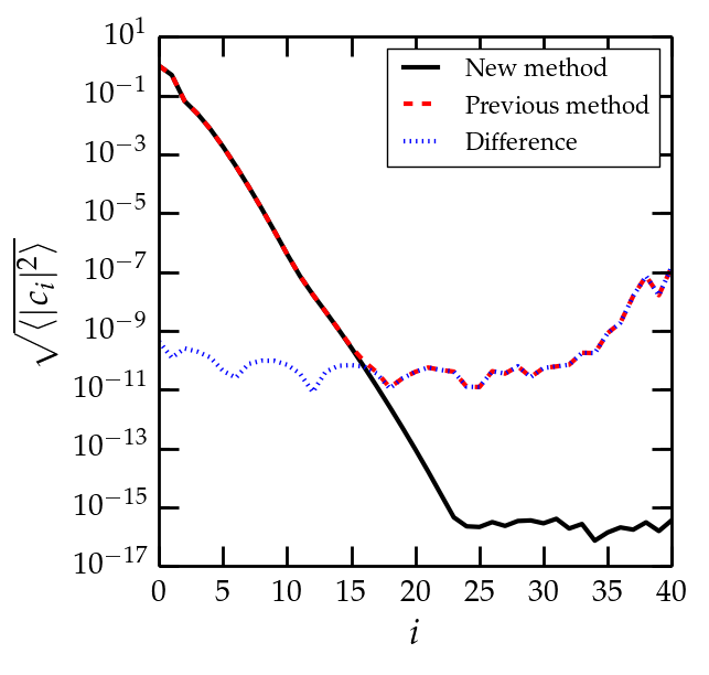
Figure 2: The angle-averaged value of the radinull spectral coefficients of $H$ after integrating Eq. (85) for the test system given in Eqs. (99)-(103) for both the new method of integration described here and the previous method introduced in Handmer and Szilágyi (2015).

To demonstrate the improvement afforded by our new method of treating the radinull integration, we test the new method of integrating Eq. (85) versus the previous method introduced in Handmer and Szilágyi (2015) on an analytic test case. Consider Eq. (85) with

$$A= \frac{.94\sin x-1.53\cos x}{R(1+x)^{2}}\ _{2}Y_{31}\ {}_{0}Y_{2-2}\ {}_{0}Y_{10},$$ (99)

$$B= -\frac{x\sin{x}}{R}\left({}_{2}Y_{3-1}+_{3}Y_{4-3}\ {}_{1}Y_{22}\right)$$

$$+\left({}_{0}Y_{00}-1\right){}_{2}Y_{22}|_{2}Y_{22}|^{2}$$ (100)

$$C= (1-\cos x)\left({}_{2}Y_{3-1}+_{1}Y_{2-2}\ {}_{1}Y_{30}\right)$$

$$+(\sin x+\cos x){}_{2}Y_{22},$$ (101)

and with $\mathcal{M}$ defined by Eqs. (83), (86), and (169) with

$$J= {}_{2}Y_{22},$$ (102)

$$T= {}_{2}Y_{22}\ {}_{0}Y_{00}.$$ (103)

For this test case, we set $R=2.94$ and we resolve the computational domain through $L=10$ and $n_{\rho}=41$. This test case is not necessarily physical, but satisfies the boundary constraint given in Eq. (95). We integrate Eq. (85) from an inner boundary value of $H_{|\Gamma}=0$ to $x=0$, obtaining $H$ as a function of $x$,$\theta$, and $\phi$, or equivalently, obtaining the radial spectral coefficients of $H$, $c_{i}(\theta_{j},\phi_{k})$ at each angular collocation point $(\theta_{j},\phi_{k})$. To reduce the size of the dataset, we average these coefficients over the sphere according to

$$\sqrt{\langle|c_{i}|\rangle}= \sum_{j,k}c_{i}(\theta_{j},\phi_{k})\bar{c_{i}}(\theta_{j},\phi_{i})\sin{\theta_{j}}\frac{2\pi^{2}}{n_{\theta}n_{\phi}},$$ (104)

and we plot these angle-averaged coefficients in Fig. 2.

Because the test case satisfies the regularity conditions, we expect that with sufficient resolution, an accurate integration scheme would be capable of resolving the solution to numerical roundoff. From Fig. 2 we see that our current method demonstrates this behavior. However, the radial modes of the previous method from Handmer and Szilágyi (2015) flattens out about 6 orders of magnitude larger, because the logarithmic terms are not properly represented via our chosen spectral decomposition.

IV.5 Time evolution

To evolve $J$ forward in time, we integrate

$$J_{,u|\rho,x^{A}=\text{const}}=\Phi$$ (105)

at each radinull point using the method of lines. This is done using an ordinary differential equation (ODE) integrator, integrating forward in $u$, with a supplied right-hand side $\Phi$. Here $\Phi$ is computed using

$$\Phi=H+\rho(1-\rho)\frac{R_{,\bar{u}}}{R}J_{,\rho},$$ (106)

where $R_{,\bar{u}}$ is the derivative of the surface area coordinate $r$ along the worldtube given by Eq. (44) and where $H$ is the result of the radinull integration, Eq. (18), accomplished using the method in Sec. IV.4.

The time integration of $J$ [Eq. (105)] uses a fifth order Dormand-Prince ODE solver with adaptive time stepping Press et al. (2007), and a default relative error tolerance of $10^{-8}$ except where otherwise noted. The step sizes are limited entirely by the error measure and is independent of the time steps of the Cauchy evolution used to generate the worldtube. The time evolution is also done in tandem with the evolution of the inertial coordinates [Eq. (134), and of the conformal factor (Eq. (117)] from $\mathscr{I}^{+}$ extraction, as described below.

V $\mathscr{I}^{+}$ Extraction

Once the characteristic equations have been solved in the volume so that the metric variables of the Bondi-Sachs form Eq. (1) are known on $\mathscr{I}^{+}$, the gravitational waveform can be computed. This involves two steps. The first step is computing the Bondi news function at $\mathscr{I}^{+}$ from the metric variables there. The second step involves transforming the news to a freely falling coordinate system at $\mathscr{I}^{+}$; this removes all remaining gauge freedom up to a BMS transformation. These steps are described below.

V.1 News function

The metric in Bondi-Sachs form given in Eq. (1) is divergent at $\mathscr{I}^{+}$ where $r\rightarrow\infty$, so we work with a conformally rescaled Bondi metric, $\hat{g}_{\mu\nu}=\ell^{2}g_{\mu\nu}$, where $\ell=1/r$, that is finite at $r\rightarrow\infty$. Expressing this metric in the coordinate system $\hat{x}^{\hat{\alpha}}=(u,\ell,x^{A})$, it takes the form Bishop et al. (1997)

$$\hat{g}_{\hat{\mu}\hat{\nu}}= -\left(e^{2\beta}(\ell^{2}+\ell W)-h_{AB}U^{A}U^{B}\right)du^{2}$$

$$+ 2e^{2\beta}dud\ell-2h_{AB}U^{B}dudx^{A}$$

$$+ h_{AB}dx^{A}dx^{B}.$$ (107)

Here $h_{AB}$, $\beta$, $W$, and $U^{A}$ are the same quantities that appear in Eq. (1).

To facilitate the computation of the news function, we construct an additional conformal metric

$$\tilde{g}_{\hat{\mu}\hat{\nu}} =\omega^{2}\hat{g}_{\hat{\mu}\hat{\nu}},$$ (108)

that is asymptotically Minkowski at $\mathscr{I}^{+}$. The conformal factor $\omega$ is chosen so that the angular part of $\tilde{g}_{\mu\nu}$ is a unit sphere metric Tamburino and Winicour (1966),

$$q_{AB}=\omega^{2}h_{AB|\mathscr{I}^{+}}.$$ (109)

In terms of the original metric,

$$\tilde{g}_{\hat{\mu}\hat{\nu}}= \Omega g_{\hat{\mu}\hat{\nu}},$$ (110)

$$\Omega= \omega\ell.$$ (111)

On a given constant $u$ slice, $\omega$ can be computed by solving an elliptic equation related to the two-dimensional (2D) curvature scalar,

$$\mathcal{R}=2\left(\omega^{2}+h^{AB}_{|\mathscr{I}^{+}}D_{A}D_{B}\ln\omega\right),$$ (112)

where $D_{A}$ is the covariant derivative associated with $h^{AB}_{|\mathscr{I}^{+}}$. Equation (112) has the effect of setting the asymptotic 2D curvature in the conformally rescaled metric to be $2$, which is the curvature of the unit sphere. Expanding out the covariant derivatives yields Bishop et al. (1997),

$$h^{AB}_{|\mathscr{I}^{+}}D_{A}D_{B}\ln\omega= \frac{1}{4}\Big{(}-2\eth^{2}\ln\omega\bar{J}-2\bar{\eth}^{2}\ln\omega J+4\bar{\eth}\eth\ln\omega K-\eth\ln\omega\eth J\bar{J}^{2}-\eth\ln\omega\eth\bar{J}J\bar{J}-2\eth\ln\omega\eth\bar{J}$$

$$+ 2\eth\ln\omega\eth K\bar{J}K+\eth\ln\omega\bar{\eth}J\bar{J}K+\eth\ln\omega\bar{\eth}\bar{J}JK-2\eth\ln\omega\bar{\eth}KJ\bar{J}+\eth J\bar{\eth}\ln\omega\bar{J}K+\eth\bar{J}\bar{\eth}\ln\omega JK$$

$$- 2\eth K\bar{\eth}\ln\omega J\bar{J}-\bar{\eth}\ln\omega\bar{\eth}JJ\bar{J}-2\bar{\eth}\ln\omega\bar{\eth}J-\bar{\eth}\ln\omega\bar{\eth}\bar{J}J^{2}+2\bar{\eth}\ln\omega\bar{\eth}KJK\Big{)}.$$ (113)

Equation (112) could in principle be used to solve for $\omega$ at each slice of constant $u$. However, we instead solve this equation for $\omega$ only on the initial slice, where the equation simplifies significantly (see below), and then we construct an evolution equation for $\omega$ and we evolve $\omega$ as a function of $u$. Note that when evolving $\omega$, one could use Eq. (112) as a check to monitor the error in $\omega$; however we do not yet do so.

On the initial slice, Eqs. (112) and (113) simplify considerably; we have set $J_{|\mathscr{I}^{+}}=0$ (see Eq. (IV.3)), so Eq. (113) implies that $h^{AB}_{|\mathscr{I}^{+}}D_{A}D_{B}\ln\omega=4\bar{\eth}\eth\ln\omega$ and Eq. (19) implies that $\mathcal{R}=2$, reducing Eq. (112) to $1=\omega^{2}+\bar{\eth}\eth\ln\omega$. This has the trivial solution of $\omega=1$.

The null generators at $\mathscr{I}^{+}$ are defined as Bishop et al. (1997),

$$\tilde{n}^{\hat{\mu}}= \tilde{g}^{\hat{\mu}\hat{\nu}}\nabla_{\hat{\nu}}\Omega_{|\mathscr{I}^{+}},$$ (114)

$$\hat{n}^{\hat{\mu}}= \hat{g}^{\hat{\mu}\hat{\nu}}\nabla_{\hat{\nu}}\ell_{|\mathscr{I}^{+}}=\hat{g}^{\hat{\mu}\ell},$$ (115)

so that

$$\tilde{n}^{\hat{\mu}}=\omega^{-1}\hat{n}^{\hat{\mu}}.$$ (116)

where the covariant derivative $\nabla_{\hat{\nu}}$ is associated with the Bondi metric, $g_{\hat{\mu}\hat{\nu}}$. Derivation for evolution of the conformal factor on $\mathscr{I}^{+}$ in the frame of the compactified metric, is given in Ref Bishop et al. (1997), and can be computed by

$$2\hat{n}^{\hat{\mu}}\nabla_{\hat{\mu}}\ln\omega=-e^{-2\beta}W_{|\mathscr{I}^{+}}.$$ (117)

Reference Bishop et al. (1997) derived the formula for the news function in the conformal metric with the evolution coordinates, with a sign error corrected in Babiuc et al. (2009) (Ref Bishop et al. (1997) chose their convention to agree with Bondi’s original expression in the axisymmetric case Bondi et al. (1962)). Here we have factored the $s_{i}$ slightly differently than they did,

$$N= \frac{1}{16\omega A(K+1)}\left(4s_{1}+2s_{2}-\left(\eth\bar{U}+\bar{\eth}U\right)s_{3}-\frac{8}{\omega^{2}}s_{4}+\frac{2}{\omega}s_{5}\right),$$ (118)

$$A= \omega e^{2\beta},$$ (119)

$$s_{1}= J^{2}\bar{H}_{,\ell}+J\bar{J}H_{,\ell}+2(K+1)\left(H_{,\ell}-JK_{,u\ell}\right),$$ (120)

$$s_{2}= \eth J_{,\ell}J\bar{J}\bar{U}+\eth\bar{J}_{,\ell}J^{2}\bar{U}+2\eth UJ\bar{J}K_{,\ell}+2\eth\bar{U}J\bar{J}J_{,\ell}+\bar{\eth}J_{,\ell}J\bar{J}U+\bar{\eth}\bar{J}_{,\ell}J^{2}U+2\bar{\eth}UJ^{2}\bar{J}_{,\ell}+2\bar{\eth}\bar{U}J^{2}K_{,\ell}$$

$$+ (K+1)\Big{(}2\eth J_{\ell}\bar{U}-2\eth K_{,\ell}J\bar{U}-2\eth UJ\bar{J}_{,\ell}+4\eth UK_{,\ell}-2\eth\bar{U}JK_{,\ell}+4\eth\bar{U}J_{,\ell}+2\bar{\eth}J_{,\ell}U-2\bar{\eth}K_{,\ell}JU$$

$$- 2\bar{\eth}UJK_{,\ell}-2\bar{\eth}\bar{U}JJ_{,\ell}\Big{)},$$ (121)

$$s_{3}= J^{2}\bar{J}_{,\ell}+J\bar{J}J_{,\ell}+2(K+1)(J_{,\ell}-JK_{,\ell}),$$ (122)

$$s_{4}= \eth A\eth\omega J\bar{J}+\bar{\eth}A\bar{\eth}\omega J^{2}+(K+1)\Big{(}2\eth A\eth\omega-\eth A\bar{\eth}\omega J-\bar{\eth}A\eth\omega J\Big{)},$$ (123)

$$s_{5}= 2\eth^{2}AJ\bar{J}+2\bar{\eth}^{2}AJ^{2}+\eth A\eth JJ\bar{J}^{2}+\eth A\eth\bar{J}J^{2}\bar{J}-\eth A\bar{\eth}JJ\bar{J}K-\eth A\bar{\eth}\bar{J}J^{2}K+2\eth A\bar{\eth}KJ^{2}\bar{J}$$

$$+ 2\bar{\eth}A\eth KJ^{2}\bar{J}+\bar{\eth}A\bar{\eth}JJ^{2}\bar{J}+\bar{\eth}A\bar{\eth}\bar{J}J^{3}-2\bar{\eth}A\bar{\eth}KJ^{2}K$$

$$+ (K+1)\Big{(}4\eth^{2}A-4\bar{\eth}\eth AJ+2\eth A\eth J\bar{J}+2\eth A\eth\bar{J}J-4\eth A\eth K+2\eth A\bar{\eth}J-2\bar{\eth}A\eth J+4\bar{\eth}A\eth KJ\Big{)}$$

$$+ (K+2)\Big{(}-2\eth A\eth KJ\bar{J}-\bar{\eth}A\eth JJ\bar{J}-\bar{\eth}A\eth\bar{J}J^{2}\Big{)}.$$ (124)

The news as defined in Eq. (118) has spin weight $+2$. However, the usual convention for gravitational radiation is to work with quantities with spin weight $-2$. Furthermore, the news $N$ has the opposite sign as the usual convention. To relate this news function to the gravitational wave strain defined using the following convention: given a radially outward propagating metric perturbation from Minkowski, $h_{\tilde{\mu}\tilde{\nu}}=g_{\tilde{\mu}\tilde{\nu}}-\eta_{\tilde{\mu}\tilde{\nu}}$ and polarizations given by $h_{+}=(h_{\tilde{\theta}\tilde{\theta}}+h_{\tilde{\phi}\tilde{\phi}})/2$ and $h_{\times}=h_{\tilde{\theta}\tilde{\phi}}$, the strain is given by

$$h=h_{+}-ih_{\times}.$$ (125)

Then the news is related to the strain by,

$$\partial_{\tilde{u}}h=2\overline{N}.$$ (126)

V.2 Inertial coordinates

Once the news function is computed according to Sec. V.1, it is known as a function of coordinates $(u,x^{A})$ on $\mathscr{I}^{+}$. Recall that these coordinates are chosen so that $u=\breve{t}$ and $x^{A}=\breve{x}^{\breve{A}}$ on the worldtube, where $(\breve{t},\breve{x}^{\breve{A}})$ are the time and angular coordinates of the interior Cauchy evolution. Therefore, the news as computed above depends on the choice of Cauchy coordinates.

In this section, we transform the news to a new inertial coordinate system $(\tilde{u},\tilde{x}^{\tilde{A}})$ on $\mathscr{I}^{+}$, where curves of constant $\tilde{x}^{\tilde{A}}$ correspond to worldlines of free-falling observers (because we are working on $\mathscr{I}^{+}$, we can suppress the radinull coordinate). This removes the remaining gauge freedom in the news, up to a choice of free-falling observers (or in other words up to a BMS transformation).

On the initial slice, we choose $\tilde{u}=u$ and $\tilde{x}^{\tilde{A}}=x^{A}$. These inertial coordinates then evolve along the $\mathscr{I}^{+}$ generators Bishop et al. (1997),

$$\hat{n}^{\mu}\partial_{\mu}\tilde{u}=\omega,$$ (127)

$$\hat{n}^{\mu}\partial_{\mu}\tilde{x}^{\tilde{A}}=0,$$ (128)

where the $\hat{n}^{\mu}$ are given by elements of the compactified metric according to Eq. (115).

Since $\tilde{x}^{\tilde{A}}=(\tilde{\theta},\tilde{\phi})$ are not representable via a spectral expansion in spherical harmonics, thus making them poor choices for our numerics, we represent the inertial coordinates using a Cartesian basis $\tilde{x}^{\tilde{\i}}=(\tilde{x},\tilde{y},\tilde{z})$. We reexpand Eq. (128), using the transformations

$$\frac{\partial\tilde{\theta}}{\partial x^{\mu}} =\frac{1}{\tilde{x}^{2}+\tilde{y}^{2}}\left(-\tilde{y}\frac{\partial\tilde{x}}{\partial x^{\mu}}+\tilde{x}\frac{\partial\tilde{y}}{\partial x^{\mu}}\right),$$ (129)

$$\frac{\partial\tilde{\phi}}{\partial x^{\mu}} =\frac{1}{\tilde{r}^{2}\sqrt{\tilde{x}^{2}+\tilde{y}^{2}}}\left(\tilde{x}\tilde{z}\frac{\partial\tilde{x}}{\partial x^{\mu}}+\tilde{y}\tilde{z}\frac{\partial\tilde{y}}{\partial x^{\mu}}-(\tilde{x}^{2}+\tilde{y}^{2})\frac{\partial\tilde{z}}{\partial x^{\mu}}\right).$$ (130)

Plugging those into Eq. (128) yields the coupled equations

$$-\tilde{y}\frac{\partial\tilde{x}}{\partial u}+\tilde{x}\frac{\partial\tilde{y}}{\partial u} =\frac{\hat{n}^{\hat{A}}}{\hat{n}^{u}}\left(-\tilde{y}\frac{\partial\tilde{x}}{\partial\hat{x}^{\hat{A}}}+\tilde{x}\frac{\partial\tilde{y}}{\partial\hat{x}^{\hat{A}}}\right),$$ (131)

$$\tilde{x}\tilde{z}\frac{\partial\tilde{x}}{\partial u}+\tilde{y}\tilde{z}\frac{\partial\tilde{y}}{\partial u}-(\tilde{x}^{2}+\tilde{y}^{2})\frac{\partial\tilde{z}}{\partial u} =\frac{\hat{n}^{\hat{A}}}{\hat{n}^{u}}\left(\tilde{x}\tilde{z}\frac{\partial\tilde{x}}{\partial\hat{x}^{\hat{A}}}+\tilde{y}\tilde{z}\frac{\partial\tilde{y}}{\partial\hat{x}^{\hat{A}}}-(\tilde{x}^{2}+\tilde{y}^{2})\frac{\partial\tilde{z}}{\partial\hat{x}^{\hat{A}}}\right).$$ (132)

By expanding the basis from two coordinates to three, we also need to introduce a constraint which will force the $\tilde{x}^{\tilde{\i}}$ to remain on the unit sphere and eliminate the extra degree of freedom, $\tilde{r}=\sqrt{\tilde{x}^{2}+\tilde{y}^{2}+\tilde{z}^{2}}=1$. While this holds analytically, numerically $\tilde{r}$ will shift away from 1 during the evolution, which makes it necessary to introduce a constraint equation to the system of equations,

$$\frac{\partial\tilde{r}}{\partial u}=\tilde{x}\frac{\partial\tilde{x}}{\partial u}+\tilde{y}\frac{\partial\tilde{y}}{\partial u}+\tilde{z}\frac{\partial\tilde{z}}{\partial u}=\tilde{r}C(\tilde{r}),$$ (133)

where $C(\tilde{r})$ is a constraint term where $C(\tilde{r}=1)=0$. In our code, $C(\tilde{r})=-\kappa(\tilde{r}-1)$ for some positive parameter $\kappa$.

With these three equations, Eqs. (131)-(133), we solve for the three $\frac{\partial\tilde{x}^{\tilde{\i}}}{\partial u}$. After some manipulations and massaging, we obtain the evolution equations for the Cartesian inertial coordinates with respect to the characteristic coordinates,

$$\frac{\partial\tilde{x}^{i}}{\partial u}=\frac{\tilde{x}^{i}}{\tilde{r}}C(\tilde{r})+\frac{1}{\tilde{r}^{2}}\left(-\tilde{x}^{i}\tilde{x}^{j}\delta_{jk}+\delta^{i}{}_{k}\tilde{r}^{2}\right)\frac{\partial\tilde{x}^{k}}{\partial\hat{x}^{\hat{A}}}\frac{\hat{n}^{\hat{A}}}{\hat{n}^{u}}.$$ (134)

Once we know $\tilde{u}(u,x^{A})$, $\tilde{x}^{\tilde{\i}}(u,x^{A})$, then obtaining the news on this grid is a matter of interpolation. Our code does so in two steps. First, each of the spatial coordinates, as well as the news function is interpolated in time onto slices of constant $\tilde{u}$, so that we then have both $\tilde{x}^{\tilde{i}}(\tilde{u},x^{A})$ and $N(\tilde{u},x^{A})=N(\tilde{u},\tilde{x}^{\tilde{\i}})$, using a cubic spline along each grid point on $\mathscr{I}^{+}$.

Then on each constant $\tilde{u}$ slice, we perform the spatial interpolation by projecting the news function onto its spectral coefficients $c^{\ell m}$, using the orthonormality of SWSHes from Eq. (162),

$$c^{\ell m}(\tilde{u})=\int_{S^{2}}N(\tilde{u},\tilde{x}^{\tilde{\i}})\overline{{}^{2}Y^{\ell m}}(\tilde{\theta},\tilde{\phi})\sin\tilde{\theta}d\tilde{\theta}d\tilde{\phi}.$$ (135)

However, since we numerically evaluate news function on the noninertial characteristic coordinates, we must instead do the integration over its area elements, $\sin\theta d\theta d\phi$, so we convert the coordinates of this expression, which introduces the determinant of a Jacobian,

$$d\tilde{\theta}d\tilde{\phi}=d\theta d\phi\left|\frac{\partial\tilde{x}^{\tilde{A}}}{\partial x^{A}}\right|.$$ (136)

Once again, because of the difficulties of representing angular coordinates spectrally, we convert this expression from $\tilde{\theta}$ and $\tilde{\phi}$ to $\tilde{x}^{\tilde{\i}}$. To facilitate our expansion to Cartesian coordinates, we introduce a temporary radial coordinates $\tilde{\mathfrak{r}}$ and $\mathfrak{r}$ on the unit sphere with $\tilde{x}^{\tilde{A}}=(\tilde{\mathfrak{r}},\tilde{\theta},\tilde{\phi})$ and $x^{A}=(\mathfrak{r},\theta,\phi)$ so that we can properly define the determinants (keeping in mind $\tilde{\mathfrak{r}}$ and $\mathfrak{r}$ are analytically identical to 1 and will disappear from the final expressions),

$$\left|\frac{\partial\tilde{x}^{\tilde{A}}}{\partial x^{A}}\right|= \left|\frac{\partial\tilde{x}^{\tilde{A}}}{\partial\tilde{x}^{\tilde{\i}}}\right|\left|\frac{\partial\tilde{x}^{\tilde{\i}}}{\partial x^{A}}\right|$$

$$= \left(\frac{1}{\tilde{\mathfrak{r}}^{2}\sin\tilde{\theta}}\right)\left|\frac{\partial\tilde{x}^{\tilde{\i}}}{\partial x^{A}}\right|.$$ (137)

Plugging everything in yields the full expression,

$$c^{\ell m}(\tilde{u})=\int_{S^{2}}N(\tilde{u},\tilde{x}^{\tilde{\i}})\overline{{}^{2}Y^{\ell m}}(\tilde{\theta},\tilde{\phi})\frac{1}{\sin\theta}\left|\frac{\partial\tilde{x}^{\tilde{\i}}}{\partial x^{A}}\right|\sin\theta d\theta d\phi.$$ (138)

Note that we have included a factor of $\sin\theta/\sin\theta$ which, while analytically trivial, aids with the numerics of our code. Incorporating the $\sin\theta$ in the numerator generates the proper spherical area element for the integration, while we factor the $1/\sin\theta$ into the $\frac{\partial}{\partial\phi}$ terms in the Jacobian, as numerically computed spherical gradients return factors of $\frac{1}{\sin\theta}\frac{\partial}{\partial\phi}$.

If the strain is similarly decomposed into spin weight $-2$ spherical harmonic coefficients, $h_{\ell m}$, then they are related to the news coefficients by,

$$\partial_{\tilde{u}}h_{\ell m}=2(-1)^{-m}\overline{c^{\ell-m}_{\text{CCE}}}.$$ (139)

One potential issue with Eq. (138) is the possibility that there is a significant drift in the inertial coordinates relative to the code coordinates. If there is a large systematic shift in the coordinates (for example, if they all drift toward a single sky location), then there could be regions on the unit sphere which are sparsely represented. Because spectral methods of computing integrals often assume an optimal distribution of grid points across the surface, this drift means there is a risk of underresolving the computation Eq. (138), especially for high $\ell$ modes. To forestall this issue, we have taken to representing the $\mathscr{I}^{+}$ extraction portion at a significantly higher angular resolution from the rest of our code. In particular, when we properly resolve the volume evolution up to $\ell_{\text{max}}$ angular modes, we maintain a basis consisting of $2\ell_{\text{max}}$ angular modes for our $\mathscr{I}^{+}$ extraction code. Our properly resolved information content is still no better than what is resolved in the volume evolution (i.e. $\ell_{\text{max}}$), but this allows us to accurately project onto the inertial coordinates with Eq. (138). Because the $\mathscr{I}^{+}$ extraction portion of the code is only a 2D surface, this choice is an insignificant contribution to the overall computational cost of our code.

While this coordinate evolution projects the news function on an inertial frame, it is not a unique inertial frame. The class of inertial observers at $\mathscr{I}^{+}$ are all related to each other by the group of BMS transformations. Because our CCE inertial coordinates at $\mathscr{I}^{+}$ correspond to free-falling observers, the BMS frame remains constant throughout the entire characteristic evolution. Thus, the BMS frame we use in our evolution is frozen in entirely by our choice to identify our inertial coordinates with the characteristic coordinates on our initial slice (i.e. $\tilde{u}=u$ and $\tilde{x}^{\tilde{A}}=x^{A}$). This choice is in some sense arbitrary, as it is ultimately related to the coordinates provided on the worldtube by the Cauchy evolution on that initial slice, and there are no guarantees of consistency between CCE evolutions on different worldtubes even from the same Cauchy evolution. However, development of a consistent treatment of handing the choice of BMS frame is beyond the scope of this paper.

V.3 Computational grid

We use Spherepack for most of the $\mathscr{I}^{+}$ Extraction, with the final projection onto the inertial coordinates done using Spinsfast. The time evolution of the inertial coordinates, Eq. (134), and of the conformal factor, Eq. (117), is done in tandem with the evolution of $J$, Eq. (106), in the volume extraction, using the same routine (fifth order Dormand-Prince) and error tolerance as specified for that evolution.

VI Code Tests

In order to showcase the accuracy, speed, and robustness of this spectral CCE code, we perform a number of tests on the code. We have two linearized solutions, a trivial analytic solution, and two fully nonlinear tests which outline how well the code can remove purely coordinate effects from the news output.

VI.1 Linearized analytic solution

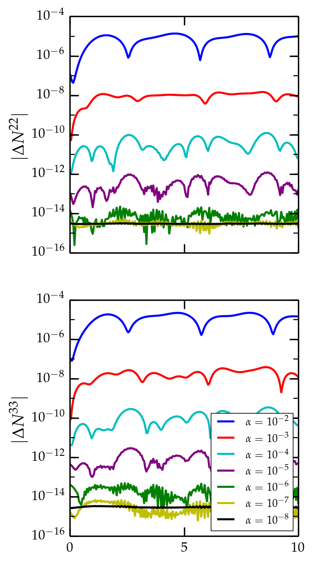
Figure 3: The difference between the numerically evolved news function and the analytic solution for the linearized analytic test of Sec. VI.1, for various amplitudes of the linear perturbation $\alpha$. The $(2,2)$ mode is on the left and the $(3,3)$ mode on the right. We expect differences of order $\alpha^{2}$ because we evolve the nonlinear terms that the linearized analytic solution neglects. For both modes, the magnitude of the differences scales as at least $\alpha^{2}$ until they approach numerical roundoff.

The linearized form for the Bondi-Sachs metric for a shell of outgoing perturbations on a Minkowski background was given in Bishop (2005), though our choice of notation follows more closely with that used in Reisswig et al. (2007). We can express the solutions in terms of the metric quantities

$$J_{\text{lin}}= \sqrt{(\ell+2)!/(\ell-2)!}\ ^{2}Z^{\ell m}\Re\left(J_{\ell}(r)e^{i\nu u}\right),$$

$$U_{\text{lin}}= \sqrt{\ell(\ell+1)}\ ^{1}Z^{\ell m}\Re\left(U_{\ell}(r)e^{i\nu u}\right),$$

$$\beta_{\text{lin}}= \ {}^{0}Z^{\ell m}\Re\left(\beta_{\ell}(r)e^{i\nu u}\right),$$

$$W_{\text{lin}}= \ {}^{0}Z^{\ell m}\Re\left(W_{\ell}(r)e^{i\nu u}\right),$$ (140)

where $\nu$ is a real constant setting the frequency of the perturbations and $J_{\ell}(r),U_{\ell}(r),\beta_{\ell}(r)$, and $W_{\ell}(r)$ are all analytic complex functions of just the radius and $\ell$-mode of the perturbation, given below. The angular content is expressed through the various ${}^{s}Z^{\ell m}$, which are just linear combinations of the typical SWSHes defined as in Bishop (2005)

$${}^{s}Z^{\ell m}= \frac{1}{\sqrt{2}}\left({}^{s}Y^{\ell m}+(-1)^{m}\ {}^{s}Y^{\ell-m}\right) \text{for }m>0,$$

$${}^{s}Z^{\ell m}= \frac{i}{\sqrt{2}}\left((-1)^{m}\ {}^{s}Y^{\ell m}-\ ^{s}Y^{\ell-m}\right) \text{for }m<0,$$

$${}^{s}Z^{\ell 0}= \ {}^{s}Y^{\ell 0}.$$ (141)

To get the linearized expression for $H_{\text{lin}}$, we can simply take a direct $u$ derivative of $J_{\text{lin}}$. Since these expressions are defined according to the Bondi metric, with the surface area coordinate $r$ (rather than $\rho$), $u$ derivatives are taken along curves of constant $r$. Thus $H_{\text{lin}}=J_{\text{lin},u}$.

From this, the linearized news function can be expressed as

$$\mathcal{N}_{\text{lin}}= \Re\left(e^{i\nu u}\lim_{r\to\infty}\left(\frac{\ell(\ell+1)}{4}J_{\ell}-\frac{i\nu r^{2}}{2}J_{\ell,r}\right)+e^{i\nu u}\beta_{\ell}\right)$$

$$\times \sqrt{\frac{(\ell+2)!}{(\ell-2)!}}\ ^{2}Z^{\ell m}.$$ (142)

Reference Reisswig et al. (2007) explicitly wrote out the solutions to the linearized evolution quantities and news function for the $\ell=2$ and $\ell=3$ modes, which we reproduce here. For $\ell=2$,

$$\beta_{2}= B_{2},$$

$$J_{2}(r)= \frac{24B_{2}+3i\nu C_{2a}-i\nu^{3}C_{2b}}{36}+\frac{C_{2a}}{4r}-\frac{C_{2b}}{12r^{3}},$$

$$U_{2}(r)= \frac{-24i\nu B_{2}+3\nu^{2}C_{2a}-\nu^{4}C_{2b}}{36}+\frac{2B_{2}}{r}+\frac{C_{2a}}{2r^{2}}$$

$$+ \frac{i\nu C_{2b}}{3r^{3}}+\frac{C_{2b}}{4r^{4}},$$

$$W_{2}(r)= \frac{24i\nu B_{2}-3\nu^{2}C_{2a}+\nu^{4}C_{2b}}{6}$$

$$+ \frac{3i\nu C_{2a}-6B_{2}-i\nu^{3}C_{2b}}{3r}$$

$$- \frac{\nu^{2}C_{2b}}{r^{2}}+\frac{i\nu C_{2b}}{r^{3}}+\frac{C_{2b}}{2r^{4}},$$

$$\mathcal{N}^{2m}= \Re\left(\frac{i\nu^{3}C_{2b}}{\sqrt{24}}e^{i\nu u}\right)\ ^{2}Z^{2m},$$ (143)

and for $\ell=3$,

$$\beta_{3}= B_{3},$$

$$J_{3}(r)= \frac{60B_{3}+3i\nu C_{3a}+\nu^{4}C_{3b}}{180}+\frac{C_{3a}}{10r}-\frac{i\nu C_{3b}}{6r^{3}}-\frac{C_{3b}}{4r^{4}},$$

$$U_{3}(r)= \frac{-60i\nu B_{3}+3\nu^{2}C_{3a}-i\nu^{5}C_{3b}}{180}+\frac{2B_{3}}{r}+\frac{C_{3a}}{2r^{2}}$$

$$- \frac{2\nu^{2}C_{3b}}{3r^{3}}+\frac{5i\nu C_{3b}}{4r^{4}}+\frac{C_{3b}}{r^{5}},$$

$$W_{3}(r)= \frac{60i\nu B_{3}-3\nu^{2}C_{3a}+i\nu^{5}C_{3b}}{15}$$

$$+ \frac{i\nu C_{3a}-2B_{3}+\nu^{4}C_{3b}}{3r}$$

$$- \frac{2i\nu^{3}C_{3b}}{r^{2}}-\frac{4i\nu^{2}C_{3b}}{r^{3}}+\frac{5\nu C_{3b}}{2r^{4}}+\frac{3C_{3b}}{r^{5}},$$

$$\mathcal{N}^{3m}= \Re\left(\frac{-\nu^{4}C_{3b}}{\sqrt{30}}e^{i\nu u}\right)\ ^{2}Z^{3m},$$ (144)

where $B_{\ell},C_{\ell a}$, and $C_{\ell b}$ are all freely chosen complex constants. Note that only the values of $C_{\ell b}$ show up in the expression for the news.

For the tests we performed here, we follow a similar setup as in Reisswig et al. (2007, 2013), where we evolve a system which is a simple linear combination of the $(2,2)$ and $(3,3)$ modes. Specifically, the parameter values are $\nu=1$, $B_{\ell}=0.5i\alpha$, $C_{\ell a}=1.5\alpha$, and $C_{2b}=-iC_{3b}=0.5\alpha$, where the constant $\alpha$ sets the amplitude of the resulting news as well as the scale of the linearity of the system. Because we evolve the entire nonlinear solution, and not just a linearized version, we expect our results to differ from the analytic solution with differences that scale as the square of the amplitude, $\alpha^{2}$.

We place these linearized values of the evolution quantities $(J,W,U,\beta)$ on a chosen worldtube to serve as the inner boundary values for the volume evolution. By starting with the worldtube in the Bondi metric, we bypass the entire inner boundary formalism since we are already starting with the Bondi metric quantities. To make this test even more demanding, we chose our worldtube such that its surface area coordinate varies both in time and across the surface, given by the formula

$$R(u,x,y,z)=5\left(1+\frac{(-0.42x+0.29y+0.09z)(0.2x+0.1y-0.12z)(0.7x+0.1y-0.3z)(0.12x-0.31y-0.5z)}{(x^{2}+y^{2}+z^{2})^{2}}\sin{\pi u}\right).$$ (145)

We chose this distortion of the surface area coordinate somewhat arbitrarily, ensuring that it had distortions with modes up through $\ell=4$ as well as a time varying component with a frequency distinct from that of the linearized perturbation. This tests the code’s ability to distinguish between $H$ and $\Phi$ with the correct handling of the moving worldtube surface area coordinate, $R$, at least to linear order. Since this test bypasses the inner boundary formalism, we cannot make any claim about whether the coordinate radius $\breve{r}$ of the worldtube is moving as there is no defined coordinate radius.

The data for $J$ on the initial slice we also read off from Eq. (140). With the worldtube metric values and initial slice established, we evolve the full characteristic system. We resolve SWSH modes through $\ell=8$ with a radinull resolution of 20 grid points and a relative time integration error tolerance of $10^{-8}$. We test the characteristic evolution against perturbation amplitudes of $\alpha=(10^{-2},10^{-3},10^{-4},10^{-5},10^{-6},10^{-7},10^{-8})$ from $u=0$ to $u=10$. We compute the difference between the computed news and the analytic results from Eq. (142), $|\Delta N^{\ell m}|=|N^{\ell m}_{\text{Char}}-\mathcal{N}^{\ell m}_{\text{lin}}|$ in Fig. 3. Note, we are examining the news function evaluated at the $\mathscr{I}^{+}$ coordinates $(u,\theta,\phi)$, rather than the inertial coordinates $(\tilde{u},\tilde{\theta},\tilde{\phi})$, because we expect the difference between the two systems to be a small correction to the linearized values.

From Fig. 3 we clearly see that when $\alpha\gtrsim 10^{-6}$, $|\Delta N^{\ell m}|$ scales as $\alpha^{2}$. When $\alpha\lesssim 10^{-6}$, the difference in news rapidly reaches a floor below $10^{-14}$ for the smallest amplitude perturbations. Modes other than $(2,\pm 2)$ and $(3,\pm 3)$ all converge toward $0$ with scaling behavior no worse than $|\Delta N^{\ell m}|\lessapprox\mathcal{O}(\alpha^{2})$ until reaching machine roundoff. The observed scaling with $\alpha$ matches the expected scaling: we are evolving the full nonlinear equations but are comparing to an analytic solution of the linearized equations.

Previous iterations of CCE codes have performed a similar linearized analytic test Babiuc et al. (2009); Reisswig et al. (2010). While their choice of parameters differs slightly from ours, they are most similar to our $\alpha=10^{-6}$, with inner boundaries at fixed, uniform $R$ worldtube surfaces. The error in their news at the resolutions they tested was worse than $10^{-10}$, whereas the error in our news for the $\alpha=10^{-6}$ case is at the order of $10^{-14}$, hovering just about the error of our numerical roundoff. While comparing our results to theirs is not exactly a 1-1 comparison, we believe this is evidence for how effective our code is at resolving the linear case.

VI.2 Teukolsky wave

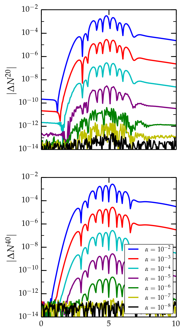
Figure 4: The difference between the numerically evolved news function and the analytic solution for the Teukolsky wave test of Sec. VI.2, for various amplitudes of the linear perturbation $\alpha$. The $(2,0)$ mode is on the left and the $(4,0)$ mode on the right. We expect differences of order $\alpha^{2}$ because we evolve the nonlinear terms that the Teukolsky wave solution neglects. For both modes, the magnitude of the differences scales as at least $\alpha^{2}$ until it approaches numerical roundoff.

A Teukolsky wave is a propagating gravitational wave in the perturbative limit of Einstein’s equations. For outgoing waves the metric has the form Teukolsky (1982)

$$d\breve{s}^{2}= -d\breve{t}^{2}+(1+\breve{f}_{rr})d\breve{r}^{2}+2B\breve{f}_{r\theta}\breve{r}d\breve{r}d\breve{\theta}$$

$$+ 2B\breve{f}_{r\phi}\breve{r}\sin\breve{\theta}d\breve{r}d\breve{\phi}+\left(1+C\breve{f}_{\theta\theta}^{(1)}+A\breve{f}_{\theta\theta}^{(2)}\right)\breve{r}^{2}d\breve{\theta}^{2}$$

$$+ 2(A-2C)\breve{f}_{\theta\phi}\breve{r}^{2}\sin\breve{\theta}d\breve{\theta}d\breve{\phi}$$

$$+ \left(1+C\breve{f}_{\phi\phi}^{(1)}+A\breve{f}_{\phi\phi}^{(2)}\right)\breve{r}^{2}\sin^{2}\breve{\theta}d\breve{\phi}^{2},$$ (146)

where the functions $\breve{f}_{ij}$ are known functions of angles listed below, and the functions $A,B,$ and $C$ are computed from the freely specifiable function $F(\breve{u})=F(\breve{t}-\breve{r})$,

$$A= 3\left(\frac{d_{\breve{u}}^{2}F}{\breve{r}^{3}}+\frac{3d_{\breve{u}}F}{\breve{r}^{4}}+\frac{3F}{\breve{r}^{5}}\right),$$

$$B= -\left(\frac{d_{\breve{u}}^{3}F}{\breve{r}^{2}}+\frac{3d_{\breve{u}}^{2}F}{\breve{r}^{3}}+\frac{6d_{\breve{u}}F}{\breve{r}^{4}}+\frac{6F}{\breve{r}^{5}}\right),$$

$$C= \frac{1}{4}\left(\frac{d_{\breve{u}}^{4}F}{\breve{r}}+\frac{2d_{\breve{u}}^{3}F}{\breve{r}^{2}}+\frac{9d_{\breve{u}}^{2}F}{\breve{r}^{3}}+\frac{21d_{\breve{u}}F}{\breve{r}^{4}}+\frac{21F}{\breve{r}^{5}}\right),$$ (147)

where $d_{\breve{u}}$ is the total derivative with respect to $\breve{u}$. The choice of $F(\breve{t}-\breve{r})$ specifies outward propagating waves, as opposed to $F(\breve{t}+\breve{r})$ which would generate ingoing waves.

Following Fiske et al. (2005); Babiuc et al. (2005), we choose the outgoing solution corresponding to the SWSH ${}^{2}Y^{20}$ mode, defining the $\breve{f}_{ij}$ from above as

$$\breve{f}_{rr}= 2-3\sin^{2}\breve{\theta},\ \breve{f}_{r\theta}=-3\sin\breve{\theta}\cos\breve{\theta},\ \breve{f}_{r\phi}=0,$$

$$\breve{f}_{\theta\theta}^{(1)}= 3\sin^{2}\breve{\theta},\ \breve{f}_{\theta\theta}^{(2)}=-1,\ \breve{f}_{\theta\phi}=0,$$

$$\breve{f}_{\phi\phi}^{(1)}= -\breve{f}_{\theta\theta}^{(1)},\ \breve{f}_{\phi\phi}^{(2)}=3\sin^{2}\breve{\theta}-1,$$ (148)

and defining the profile of the waves with $F(\breve{u})=\alpha e^{-\breve{u}^{2}/\tau^{2}}$, where $\alpha$ and $\tau$ are the amplitude and width of the wave, respectively. This is slightly different from the choice of $F(\breve{u})$ used in either Fiske et al. (2005) or Babiuc et al. (2005).

Because this solution starts with a metric that is not in Bondi-Sachs form, this test utilizes the full inner boundary formalism, in contrast to the linearized analytic test in Sec. VI.1, which tests only the characteristic evolution. We evaluate the components of the metric [see Eq. (146)] at a worldtube of constant radius, $\breve{r}_{|\Gamma}$. The worldtube treatment in Sec. III assumes that the metric is given by the 3+1 variables $\breve{g}_{ij}$, $\breve{\alpha}$, and $\breve{\beta}^{i}$ in Cartesian coordinates; we obtain these 3+1 Cartesian quantities from the spherical components in Eq. (146) in the standard way, using $\breve{x}=\breve{r}\sin\breve{\theta}\cos\breve{\phi}$ and so on.

Given the metric and its derivatives evaluated on a worldtube, the inner boundary formalism creates a correspondence between time and angular coordinates on the worldtube and at $\mathscr{I}^{+}$, i.e. $(u=\breve{t},\theta=\breve{\theta},\phi=\breve{\phi})$. With that in mind, the news function of this waveform at $\mathscr{I}^{+}$ is given by the formula Babiuc et al. (2005)

$$\mathcal{N}=-\frac{3\sin^{2}\breve{\theta}}{4}\partial_{u}^{5}F(\breve{u}),$$ (149)

where $\breve{u}=u-\breve{r}_{|\Gamma}$. For our choice of $F(\breve{u})$,

$$\mathcal{N}^{20}= \alpha\sqrt{\frac{6\pi}{5}}e^{-\breve{u}^{2}}\left(120\breve{u}-160\breve{u}^{3}+32\breve{u}^{5}\right)$$ (150)

with all other news modes $\mathcal{N}^{\ell m\neq 20}=0$. When we compare our computed news with this analytic news, we do so using the news evaluated on the coordinates $(u,\theta,\phi)$, rather than the inertial ones $(\tilde{u},\tilde{\theta},\tilde{\phi})$.

Because this is a solution of the linearized Einstein equations, comparing with our numerical solution of the full nonlinear equations should yield differences that scale like $\alpha^{2}$. Note that even though we represent the magnitude of the linear perturbation with $\alpha$ in both this test and the linearized analytic test above, the absolute amplitude for a given $\alpha$ is not the same for the two tests. The Teukolsky wave news function here is over 2 orders of magnitude larger than the linearized analytic solution for the same value of $\alpha$.

For our test, the worldtube is at a coordinate radius of $\breve{r}_{|\Gamma}=5$, and we start the wave at the origin with a width of $\tau=1$ with amplitudes $\alpha=(10^{-2},10^{-3},10^{-4},10^{-5},10^{-6},10^{-7},10^{-8})$. The CCE code is run to resolve the news up through $\ell=8$ modes with 20 radinull points and a relative time integration error tolerance of $\approx 4\times 10^{-6}$. We evolve the system from $u=0$ through $u=10$, which starts and ends when the metric is effectively flat.

We show the difference between the numerical evolution and the $(2,0)$ mode of the analytic news from Eq. (150), $|\Delta N^{20}|=|N^{20}_{\text{CCE}}-\mathcal{N}^{20}|$ on the left side of Fig. 4. We see for larger perturbations ($\alpha\gtrsim 10^{-6}$) the difference in the news scales with $\alpha^{2}$, while for smaller perturbations $(\alpha\lesssim 10^{-6})$ $|\Delta N^{20}|$ reaches a floor below $10^{-12}$. For other $\ell=$ even, $m=0$ modes, such as the $(4,0)$ mode plotted on the right half of Fig. 4, the behavior is similar. Because we chose a solution with $m=0$, all $m\neq 0$ modes of the numerical solution vanish to numerical roundoff for all $\alpha$.

This behavior is very similar to what we see for the linearized analytic test. This confirms that our CCE code is consistent with the linear solution. Because this test also incorporates the full inner boundary formalism (as opposed to the linearized analytic test which does not), this also confirms that to linear order, we reproduce the Bondi metric on the worldtube.

VI.3 Rotating Schwarzschild

Following the test used in Bishop et al. (1997), we generate data corresponding to the Schwarzschild metric in Eddington-Finkelstein coordinates with a rotating coordinate transformation, $\breve{\phi}\rightarrow\breve{\phi}+\omega\breve{u}$, so the metric is

$$d\breve{s}^{2}= -\left(1-\frac{2M}{\breve{r}}-\omega^{2}\breve{r}^{2}\sin^{2}\breve{\theta}\right)d\breve{u}^{2}-2d\breve{u}d\breve{r}$$

$$+ 2\omega\breve{r}^{2}\sin^{2}\breve{\theta}d\breve{u}d\breve{\phi}+\breve{r}^{2}\sin^{2}\breve{\theta}d\breve{\Omega}^{2},$$ (151)

where $M$ is the mass, $\omega$ is the parameter of the transformation, and $\breve{u}$ is the coordinate $\breve{u}=\breve{t}-\breve{r}^{*}$. For our test, we chose $M=1$ and $\omega=0.1$. The worldtube has a radius of $\breve{r}=3M$ and the solution is evolved from $u=0M$ to $u=0.5M$. Because the metric is just Schwarzschild in different coordinates, there is no gravitational radiation. We ran our code with an $\mathit{absolute}$ time integration error tolerance of $10^{-12}$ and an inertial coordinate damping parameter of $\kappa=10$. The resulting numerical values of all the news modes (resolved up through $\ell=8$) are below absolute values of $10^{-12}$. Because this case uses a spacetime metric that is not in Bondi form and has a nontrivial angular dependence, it is a full, nonlinear test of our code (albeit with no time dependence) from the inner boundary formalism through the extraction of the news function at $\mathscr{I}^{+}$.

VI.4 Bouncing black hole

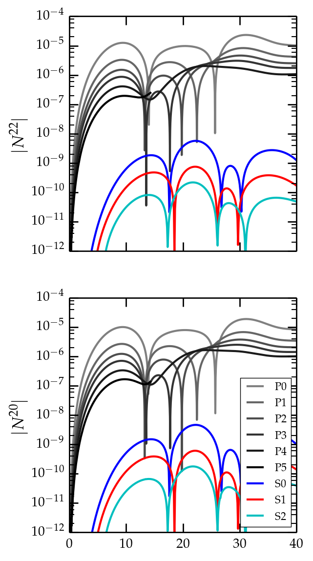
Figure 5: The absolute values of the $(2,2)$ and $(2,0)$ news modes for both the SpEC (color, resolutions denoted by S0 through S2) and PittNull (grayscale, resolutions denoted by P0 through P5) CCE codes for the bouncing black hole test (Sec. VI.4). For this test the news should be zero. Although both codes are convergent, the SpEC results achieve much smaller errors than the PittNull results, especially near the beginning and end of the cycle as the off-center translation vanishes.

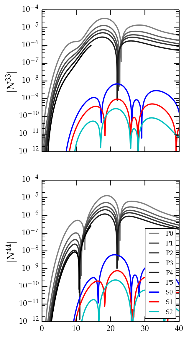
Figure 6: Same as Fig. 5, but for the $(3,3)$ and $(4,4)$ modes of the news. For these modes, the SpEC news is at least two orders of magnitude smaller than that of PittNull.

One expected key feature of CCE is its ability to remove gauge effects from the resulting waveform regardless of the coordinates of the Cauchy metric. We construct a test similar to those in Babiuc et al. (2005); Reisswig et al. (2010). We start with a Schwarzschild black hole and apply a simple time-dependent periodic coordinate translation on the spacetime. Doing so produces a time-dependent, periodic metric at the (coordinate-stationary) worldtube, but because this black hole is not radiating, the news function of this spacetime should be zero; the goal of this test is to verify that we indeed get zero in this nonlinear, time-dependent situation.

Specifically, the solution is that of a Schwarzschild black hole with mass $M=1$ in Kerr-Schild coordinates $(\breve{t},\breve{x},\breve{y},\breve{z})$, with a simple oscillating coordinate transformation

$$\breve{x}\rightarrow\breve{x}+a\sin^{4}\left(\frac{2\pi\breve{t}}{b}\right),$$ (152)

where in our test we chose $a=2M$ and $b=40M$. Thus, in the coordinate frame, which is also the frame of the worldtube, the black hole will appear to bounce back and forth along the $\breve{x}$-axis, but there is no radiated gravitational wave content. The worldtube is placed at $\breve{r}_{\Gamma}=15M$, which is intentionally very small compared to what would be used for a compact binary simulation (typically hundreds of $M$); we chose an artificially small worldtube to produce an extremely difficult test of the CCE code. We evolve the system from $u=0M$ to $u=40M$, one full period of the coordinate oscillation, starting and ending when the coordinates of the black hole are at the origin.

We performed the characteristic evolution with our spectral code at three different resolutions, which we label as S$k$, where $k$ is $(0,1,2)$. We set the resolution at each level of refinement as follows: we retain SWSH modes ${}^{s}Y^{\ell m}$ through $\ell_{\text{max}}=8+2k$, we use $20+2k$ collocation points in the radinull direction, and the adaptive time stepper uses a relative error tolerance of $3\times 10^{-5}\times e^{-k}$ with a maximum step size of $\Delta u=0.1$. For each resolution, we ran our code on a single core on the $Wheeler$ cluster at Caltech an Intel Xeon E5-2680, taking less than $(30,50,120)$ minutes for the (S0, S1, S2) resolutions, respectively.

For simplicity, we examine the news at $\mathscr{I}^{+}$ in the coordinates $(u,\theta,\phi)$ rather than in the inertial coordinates $(\tilde{u},\tilde{\theta},\tilde{\phi})$. Similarly, we expand the news into spherical harmonic modes ${}^{2}Y^{\ell m}(\theta,\phi)$. Since the news function is supposed to be zero uniformly, simple coordinate transformations at $\mathscr{I}^{+}$ are not expected to affect the overall results presented here.

As a baseline for comparison, we also ran the PittNull code on the same worldtube data. We ran PittNull at multiple resolutions (P0-P5). These correspond to a resolution of $(100^{3},200^{2},300^{3},400^{3},600^{3},900^{3})$ spatial points and fixed time steps of $\Delta u=(0.05,0.025,0.01667,0.0125,0.00833,0.00556)M$. Because PittNull takes significant computational resources at high resolution, we intentionally terminated the P5 simulation after less than $15M$. During the time that it ran, that simulation continued trends seen in the lower resolution PittNull simulations. The PittNull resolutions (P0, P1, P2) were run on 24 cores on the $Wheeler$ cluster at Caltech, taking approximately (850, 2650, 5350) total CPU hours, respectively, while resolutions (P3, P4, P5) were run on 512 cores on the BlueWaters cluster, taking approximately (9000, 17000, 24000) total CPU hours, respectively. In the case of P5, that corresponds to the cost expended on the simulation before we terminated it. This massive discrepancy on computational costs between the two codes demonstrates the impressive speed-up achieved by utilizing spectral methods, similar to what was observed with the previous implementation of this spectral code Handmer and Szilágyi (2015); Handmer et al. (2015).

In Figs. 5 and  6, we plot the amplitudes of the $(2,2),(2,0),(3,3)$, and $(4,4)$ modes of the news for both codes for all resolutions for one oscillation period. In both codes, the amplitude of the $\ell+m=$ odd modes vanishes except for numerical roundoff, likely due to the planar symmetry of the system. For the $\ell+m=$ even modes the computed numerical news is nonzero for both codes at finite resolution.

We see in Fig. 5 that for the $\ell=2$ modes the SpEC code does a better job than the PittNull code does at removing the gauge effects from the news function, at our chosen resolutions. This is especially true at the beginning and end of the oscillations when the difference between the shifted coordinates and Schwarzschild is minor.

During the middle of the period, when the coordinate effects on the worldtube metric are the largest, the difference between the SpEC and PittNull news in the $(2,2)$ and $(2,0)$ modes is the smallest. Yet even in this regime, the lowest resolution SpEC simulation improves on the highest resolution PittNull simulation by over an order of magnitude. For the higher order modes, like the $(3,3)$ or $(4,4)$ modes in Fig. 6, the peak errors in the lowest resolution SpEC results are roughly 2 orders of magnitude better than those of PittNull. In all the modes, improving the SpEC CCE resolution reduces the amplitude of the news, suggesting the remaining errors in the SpEC results are due to finite numerical resolution, rather than any issue inherent to the code.

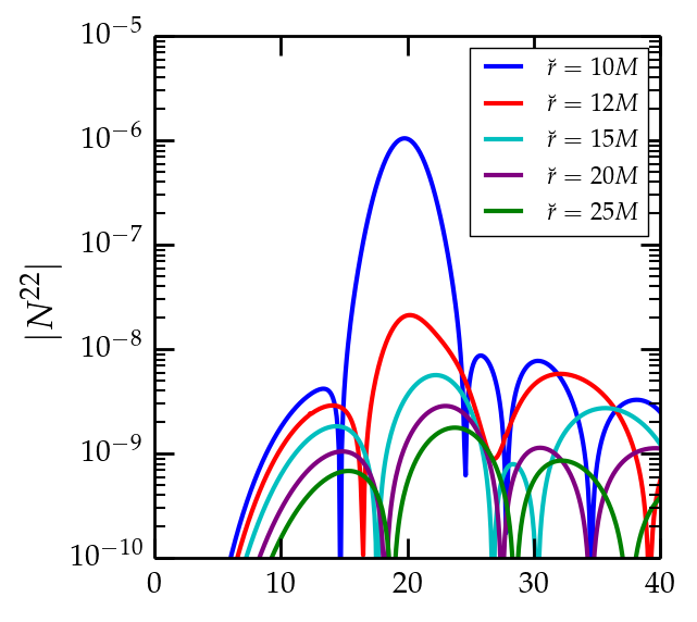
Figure 7: The absolute values of the $(2,2)$ news modes from our SpEC code at the lowest numerical resolution $S1$, for the bouncing black hole test at different coordinate worldtube radii $\breve{r}$.

This test is a rather extreme test of the code’s ability to distinguish coordinate effects, with the black hole moving an appreciable fraction of the worldtube’s radius in its coordinate frame. We also ran our code at the lowest resolution on this identical system while placing the worldtube radius at a series of different coordinate values, $\breve{r}_{|\Gamma}\in(10,12,15,20,25)M$, spread quasi-uniformly in $1/\breve{r}$. In Fig. 7, we plot the amplitude of our code’s $(2,2)$ mode for each of these worldtube radii.

Moving the worldtube to smaller radii raises the error as might be expected; eventually if the worldtube is close enough to the BH we expect caustics to form (i.e. radially outward null rays cross paths) and the characteristic formulation to fail. There is a clear convergence of this error to zero as we move the worldtube farther away and the relative size of the coordinate transformation of the bouncing BH shrinks.

VI.5 Gauge wave

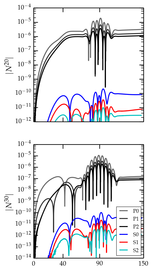
Figure 8: The amplitude of the $(2,0)$ and $(3,0)$ modes of the news for SpEC (color) and PittNull (grayscale) CCE codes, for the gauge wave test (Sec. VI.5). The center of the coordinate shift off-center occurs around $u=40M$ while the peak of the gauge wave propagates to $\mathscr{I}^{+}$ at $u=90M$. For this test, the news should be zero. At all times, the SpEC code is orders of magnitude more accurate than the PittNull code.

The bouncing black hole test is a measure of the code’s ability to remove coordinate effects resulting from simple translations; we now introduce a test to examine the code’s ability to distinguish between outgoing gravitational waves and gauge waves propagating along null slices. To generate this gauge wave, we construct a metric similar to that introduced by Eq. (5.2) in Ref Zhang et al. (2012), except modified for an outward propagating gauge transformation. Starting with the Schwarzschild metric in ingoing Eddington-Finkelstein coordinates, we apply the transformation of $\breve{v}=\breve{t}+\breve{r}+F(\breve{t}-\breve{r})/\breve{r}$ where $F(\breve{u})$ is an arbitrary function. The line element is

$$d\breve{s}^{2}= -\left(1-\frac{2M}{\breve{r}}\right)\left(1+\frac{d_{\breve{u}}F}{\breve{r}}\right)^{2}d\breve{t}^{2}+2\left(1+\frac{d_{\breve{u}}F}{\breve{r}}\right)\left(\frac{2M}{\breve{r}}+\left(1-\frac{2M}{\breve{r}}\right)\left(\frac{d_{\breve{u}}F}{\breve{r}}+\frac{F}{\breve{r}^{2}}\right)\right)d\breve{t}d\breve{r}$$

$$+ \left(1-\frac{d_{\breve{u}}F}{\breve{r}}-\frac{F}{\breve{r}^{2}}\right)\left(1+\frac{2M}{\breve{r}}+\left(1-\frac{2M}{\breve{r}}\right)\left(\frac{d_{\breve{u}}F}{\breve{r}}+\frac{F}{\breve{r}^{2}}\right)\right)d\breve{r}^{2}+\breve{r}^{2}d\breve{\Omega}^{2}.$$ (153)

Here $M$ is the mass of the black hole and $d_{\breve{u}}$ is the total derivative with respect to $\breve{u}$. For the test, we set $M=1$ and we chose $F$ to be a sine-Gaussian,

$$F(\breve{u})=\alpha\sin\left(w\breve{u}+p_{0}\right)e^{-\frac{(\breve{u}-\breve{u}_{0})^{2}}{k^{2}}}.$$ (154)

Here $\alpha$ is the amplitude of the gauge wave, $w$ is the frequency, $p_{0}$ is the initial phase offset, $\breve{u}_{0}$ is the time when the peak is at the origin, and $k$ is its characteristic width. For our test, we choose $\alpha=M$, $w=0.5/M$, $p_{0}=0.01$, $\breve{u}_{0}=40M$, and $k=10$.

Because this system is spherically symmetric, most of the terms in the evolution equations are trivially zero. In order to make the test more stringent and to generate nonzero terms in the evolution equations, we also apply an additional translation to displace the center of the black hole from the center of the worldtube. The translation used is

$$\breve{z}\rightarrow\breve{z}+2\left(1-e^{-(\breve{t}/40)^{4}}\right).$$ (155)

By moving the system entirely along the $\breve{z}$-axis, we expect only $m=0$ modes to be excited. We choose the worldtube radius to be $\breve{r}_{\Gamma}=50M$. Our gauge wave is configured so that the peak will propagate outwards and pass through this worldtube at $\breve{t}=90M$.

We ran our SpEC CCE code at three different resolutions, S$k$, for $k=(0,1,2)$. This corresponds to angular resolution of $\ell_{\text{max}}=8+2k$, radinull resolution of $20+2k$ and $\mathit{absolute}$ time integration error tolerance of $10^{-12}e^{-k}$. The three resolutions, (S0, S1, S2) were run on a single core on Caltech’s Wheeler cluster for approximately $(35,75,165)$ minutes.

PittNull CCE was also run at three resolutions, $P0$-$P2$ corresponding to a finite differencing grid with $(100^{3},200^{3},300^{3})$ spatial points and fixed times steps of size $\Delta u=(0.05,0.025,0.01667)M$. Each resolution was run on 256 cores on the BlueWaters cluster, costing approximately (1100, 3200, 6000) CPU hours.

In Fig. 8, we plot the amplitude of the $(2,0)$ and $(3,0)$ news modes for both codes and in both modes. We expect the news to be zero because the solution is merely Schwarzschild in moving coordinates. At all times both codes show convergence toward zero, with SpEC several orders of magnitude below PittNull. In the SpEC results, at the times corresponding to the coordinate shift, we see the amplitude of the news is noticeably smaller than seen in the bouncing black hole test, consistent with the larger worldtube radius used in this test. The passing gauge wave also leaves an imprint on the news that is appropriately vanishing with resolution.

Examining the higher $\ell$ modes yields a similar picture for both codes just at slightly decreasing amplitudes, as seen in the right panel of Fig. 8. Also, as expected by the axisymmetry of the setup for this test, both codes produce zero news to numerical roundoff for all $m\neq 0$ modes.

VII Conclusion

In this paper, we have detailed the implementation of our spectral CCE code as a means of extracting gravitational wave information from an interior Cauchy evolution of a relativistic system. We summarized the full theoretical framework CCE along with discussion of the changes made to the previous version of the code Handmer and Szilágyi (2015); Handmer et al. (2015). In particular, beyond bug fixes and miscellaneous alterations to the code, we have improved the numerical treatment of the poles contained within the $Q$, $W$, and $H$ evolution equations, switched the time stepper from fixed step size to a fifth order adaptive, changed the representation of the inertial coordinates at $\mathscr{I}^{+}$ for better spectral handling. All of these cumulative effects lead to a more robust and accurate code than before. This paper also clarifies a number of analytic subtleties and paper typos present within Handmer and Szilágyi (2015); Handmer et al. (2015).

We applied our code to a number of analytic test cases in order to examine its efficacy to extract the correct gravitational wave content from the worldtube data. In the pair of linearized test cases, the code successfully reproduces the analytic solution to linear order, with their differences scaling as expected (i.e. scaling by the nonlinear terms unaccounted for by the linear approximations). In these two tests, the code is ultimately limited by the numerical truncation limit of using double precision. A third test, a Schwarzschild black hole in a rotating coordinate frame, is a full nonlinear test of the code with a straightforward vanishing solution. Similar to the linear tests, the code resolves this solution up to numerical truncation limits.

The other two tests, the bouncing black hole and the gauge wave, are more rigorous tests of the code’s capability of eliminating gauge effects from the final output, and are successful at doing so. For these tests, the errors are small and convergent with resolution. Furthermore, as the worldtube boundary is placed farther from the black hole, less resolution is needed to attain a given level of error.

Overall, this version of the code shows marked improvements from the previous standards set by the PittNull code. In both the bouncing black hole and gauge wave tests, we ran PittNull at a series of different resolutions to serve as an independent comparison. The resulting news output from our code, for tests where the news should be zero, was orders of magnitude smaller than that of PittNull. In addition, we still observe the computational speed-up of our code by a factor of $>100$ that had been noted in Handmer and Szilágyi (2015); Handmer et al. (2015).

Our current goal is to run our CCE code on the catalog of SpEC waveforms Boyle et al. (2019); SXS Collaboration . In future work, we plan to couple the CCE code to run concurrently with the SpEC Cauchy evolution. Then CCE would not have to be run as a separate postprocessing step to generate the final waveforms. We would then like to follow that with Cauchy-characteristic matching (CCM) Bishop et al. (1998), whereby information from the Bondi metric is fed back into the Cauchy domain as both the Cauchy and the characteristic systems are jointly evolved. The characteristic evolution would then couple directly with the Cauchy evolution, removing the need for boundary conditions at the artificial outer boundary of the Cauchy domain. While a previous code has successfully performed CCM in the linearized case, they were unable to stably run it for the general case Szilágyi et al. (2000).

VIII Acknowledgments

We thank Leo Stein, Casey Handmer, Harald Pfeiffer, Jeff Winicour, and Saul Teukolsky for helpful advice and many useful discussions about various aspects of this project. This work was supported in part by the Sherman Fairchild Foundation and by NSF Grants No. PHY-1708212 and No. PHY-1708213 at Caltech. Computations were performed on the Wheeler cluster at Caltech, which is supported by the Sherman Fairchild Foundation and by Caltech, and on NSF/NCSA BlueWaters under allocation NSF PRAC-1713694. This research is part of the BlueWaters sustained-petascale computing project, which is supported by the National Science Foundation (Awards No. OCI-0725070 and No. ACI-1238993) and the state of Illinois. BlueWaters is a joint effort of the University of Illinois at Urbana-Champaign and its National Center for Supercomputing Applications.

Appendix A Spin-Weighted Spherical Harmonics

Spin-weighted spherical harmonics (SWSH) are a generalization of the typical spherical harmonics by introducing spin-weight raising ($\eth$) and lowering operators ($\bar{\eth}$) Newman and Penrose (1966); Goldberg et al. (1967). These derivative operators are defined by contracting the dyads with the angular derivative operator. For any spin-weighted scalar quantity $v=q_{1}^{A_{1}}\ldots q_{2}^{A_{2}}v_{A_{1}\ldots A_{n}},$ where each $q_{i}$ may be either $q$ or $\bar{q}$, we define the spin-weighted derivatives,

$$\eth v=q_{1}^{A_{1}}\ldots q_{n}^{A_{n}}q^{B}D_{B}v_{A_{1}\ldots A_{n}},$$ (156)

$$\bar{\eth}v=q_{1}^{A_{1}}\ldots q_{n}^{A_{n}}\bar{q}^{B}D_{B}v_{A_{1}\ldots A_{n}},$$ (157)

where $D$ is the angular covariant derivative on the unit sphere. By contracting these dyads with the tensor component gives the spin-weighted version of the quantities, computed above in Eqs. (8)-(11). The dyads contracted with a given quantity determine its spin weight, with $+1$ for each $q^{A}$, $-1$ for each $\bar{q}^{A}$. For example, the spin weight of $\eth\bar{J}=\frac{1}{2}\partial_{A}h_{BC}q^{A}\bar{q}^{B}\bar{q}^{C}$ is $-1$. Thus we see that $(K,\beta,W)$ have spin weight of 0, $(Q,U)$ have spin weight 1, and $(J,H,\Phi)$ have spin weight 2.

Now we can also express $\eth$ as a complex spherical derivative operator on a given quantity $F$ with a spin weight of $s$, and for our choice of dyad given in Eq. (4),

$$\eth F= -\sin^{s}\theta\left(\frac{\partial}{\partial\theta}+\frac{i}{\sin\theta}\frac{\partial}{\partial\phi}\right)(\sin^{-s}\theta F),$$ (158)

$$\bar{\eth}F= -\sin^{-s}\theta\left(\frac{\partial}{\partial\theta}-\frac{i}{\sin\theta}\frac{\partial}{\partial\phi}\right)(\sin^{s}\theta F).$$ (159)

While PittNull used a finite difference formulation for computing these derivatives Gómez et al. (1997), our code will make use of how $\eth$ acts on individual SWSH modes,

$$\eth~{}^{s}Y^{\ell m}= \sqrt{(\ell-s)(\ell+s+1)}~{}^{s+1}Y^{\ell m}$$ (160)

$$\bar{\eth}~{}^{s}Y^{\ell m}= -\sqrt{(\ell+s)(\ell-s+1)}~{}^{s-1}Y^{\ell m}$$ (161)

With this, we can start from the regular spherical harmonics ($s=0$) and build up the SWSH modes for arbitrary spin weight.

And just like regular spherical harmonics, we can take an arbitrary spin-weighted function of and decompose into spectral coefficients with the use of the expression of orthonormality of the SWSHes over the unit sphere,

$$\int_{S^{2}}~{}^{s}Y^{\ell m}~{}\overline{{}^{s}Y^{\ell^{\prime}m^{\prime}}}d\Omega= \delta_{\ell\ell^{\prime}}\delta_{mm^{\prime}},$$ (162)

where $d\Omega$ is the area element of the unit sphere $S^{2}$. Thus, given a spin-weighted quantity, we can decompose it as a sum of SWSH modes and take $\eth$ and $\bar{\eth}$ derivatives by applying the properties of Eqs. (160) and (161) to the spectral coefficients.

Last, we list some basic, useful properties of SWSHes:

1. It is only possible to add together spin-weighted quantities of identical spin weight.

2. The spin weight of a product of two SWSHes is the sum of their individual spin weights.

3. Because typical spherical harmonics are more generally SWSHes of spin weight 0, SWSHes inherit the same mode properties of spherical harmonics (i.e. $\ell\geq 0,|m|\leq\ell$).

4. In addition, the spin weight serves as a lower bound on possible $\ell$ modes, $\ell\geq|s|$.

5. The $\eth$ and $\bar{\eth}$ operators do not commute as, given spin-weighted quantity $F$ of spin $s$, $\bar{\eth}\eth F=\eth\bar{\eth}F+2sF$.

We utilize two external code packages to assist with the numerical implementation for the angular basis function, Spherepack Boyd (1989); Adams and Swarztrauber for the standard spherical harmonics and Spinsfast Huffenberger, Kevin M and Wandelt, Benjamin D (2010) for the SWSHes. In particular, we use Spherepack primarily during the inner boundary formalism and partially during $\mathscr{I}^{+}$ extraction, while we use Spinsfast during the volume evolution and $\mathscr{I}^{+}$ extraction.

Appendix B Nonlinear Evolution Equations

The full system of nonlinear equations appears below. The equations are the radinull equations on the null hypersurface for a given time slice. Reference Bishop et al. (1996) computed these full nonlinear expressions and first expressed them as SWSH quantities in Bishop et al. (1997), although we follow Handmer and Szilágyi (2015) by writing them in terms of the compactified coordinate $\rho$,

$$\beta_{,\rho}= \frac{\rho(1-\rho)}{8}\left(J_{,\rho}\bar{J}_{,\rho}-K_{,\rho}^{2}\right),$$ (163)

$$\left(r^{2}Q\right)_{,\rho}= \frac{1}{(1-\rho)^{2}}\bigg{[}R^{2}\rho^{2}\left(\vphantom{\frac{1}{2K^{2}}}2\eth\beta_{,\rho}-K\eth K_{,\rho}-K\bar{\eth}J_{,\rho}+\eth\left(\bar{J}J_{,\rho}\right)+\bar{\eth}\left(JK_{,\rho}\right)-J_{,\rho}\bar{\eth}K\right.$$

$$\left.\hphantom{\frac{1}{(1-\rho)^{2}}}\vphantom{\bar{J}^{2}}+\frac{1}{2K^{2}}\left(\eth\bar{J}(J_{,\rho}-J^{2}\bar{J}_{,\rho})+\eth J(\bar{J}_{,\rho}-\bar{J}^{2}J_{,\rho})\right)\right)\bigg{]}$$

$$+ \frac{1}{(1-\rho)^{3}}\left(-4R^{2}\rho\eth\beta\right),$$ (164)

$$U_{,\rho}= \frac{e^{2\beta}}{R\rho^{2}}\left(KQ-J\bar{Q}\right),$$ (165)

$$\mathcal{R}= 2K-\eth\bar{\eth}K+\frac{1}{2}\left(\bar{\eth}^{2}J+\eth^{2}\bar{J}\right)+\frac{1}{4K}\left(\bar{\eth}\bar{J}\eth J-\bar{\eth}J\eth\bar{J}\right),$$ (166)

$$\left(r^{2}W\right)_{,\rho}= \frac{1}{(1-\rho)^{2}}\left(\vphantom{\frac{R^{2}}{2}}-R+\frac{R^{2}\rho^{2}}{4}(\eth\bar{U}_{,\rho}+\bar{\eth}U_{,\rho})-e^{-2\beta}\frac{R^{3}\rho^{4}}{8}(2KU_{,\rho}\bar{U}_{,\rho}+J\bar{U}_{,\rho}^{2}+\bar{J}U_{,\rho}^{2})\right.$$

$$\hphantom{\frac{1}{(1-\rho)^{2}}}\left.+\frac{Re^{2\beta}}{2}\left(\mathcal{R}-2K(\eth\beta\bar{\eth}\beta+\eth\bar{\eth}\beta)+J\bar{\eth}\beta^{2}+\bar{J}\eth\beta^{2}-\eth\beta(\bar{\eth}K-\eth\bar{J})-\bar{\eth}\beta(\eth K-\bar{\eth}J)\right.\right.$$

$$\left.\left.\hphantom{\frac{1}{(1-\rho)^{2}}+Re^{2\beta}}+J\bar{\eth}^{2}\beta+\bar{J}\eth^{2}\beta\right)\vphantom{\frac{Re^{2\beta}}{2}}\right)$$

$$+ \frac{1}{(1-\rho)^{3}}\left(R^{2}\rho(\eth\bar{U}+\bar{\eth}U)\right).$$ (167)

The evolution equation of $J$ is given by $H=J_{,u|r=\text{const}}$,

$$(rH)_{,\rho}-\frac{rJ}{2}(H\bar{T}+\bar{H}T)=H_{A}+\frac{H_{B1}+H_{B2}+H_{B3}+H_{B4}}{1-\rho}+\frac{H_{C}}{(1-\rho)^{2}},$$ (168)

where

$$T= \left(J_{,\rho}-\frac{JK_{,\rho}}{K}\right),$$ (169)

$$H_{A}= (1-\rho)J_{,\rho}+\frac{R}{2}\rho^{2}W_{,\rho}J_{,\rho}+\frac{\rho}{2}(1-\rho+R\rho W)J_{,\rho\rho}-4J\beta_{,\rho},$$ (170)

$$H_{B1}= \frac{R\rho}{4}\left((6-4\rho)WJ_{,\rho}-16JW\beta_{,\rho}-\eth J\bar{U}_{,\rho}-\bar{\eth}JU_{,\rho}-2K\eth U_{,\rho}-J_{,\rho}\left(\eth\bar{U}+\bar{\eth}U\right)+J\left(\bar{\eth}U_{,\rho}-\eth\bar{U}_{,\rho}\right)\right),$$ (171)

$$H_{B2}= \frac{R\rho}{4}\left(\left(\bar{U}\eth J+U\bar{\eth}J\right)\left(J\bar{J}_{,\rho}-\bar{J}J_{,\rho}\right)-2\bar{U}\eth J_{,\rho}-2U\bar{\eth}J_{,\rho}\right.$$

$$\hphantom{\frac{R\rho}{4}}+\left.2\left(KJ_{,\rho}-JK_{,\rho}\right)\left(\bar{U}\eth K+U\bar{\eth}K+K(\bar{\eth}U-\eth\bar{U})+J\bar{\eth}\bar{U}-\bar{J}\eth U\right)\right),$$ (172)

$$H_{B3}= \frac{e^{2\beta}}{2\rho}\left((2+J\bar{J})\left(\eth^{2}\beta+\eth\beta^{2}\right)+J^{2}\left(\bar{\eth}^{2}\beta+\bar{\eth}\beta^{2}\right)-2JK\left(\eth\bar{\eth}\beta+\bar{\eth}\beta\eth\beta\right)+J\left(\eth K\bar{\eth}\beta-\eth\beta\bar{\eth}K+\eth\bar{J}\eth\beta\right)\right.$$

$$\left.\hphantom{\frac{e^{2\beta}}{2\rho}}+\bar{J}\eth J\eth\beta+K\left(\bar{\eth}J\eth\beta-\eth J\bar{\eth}\beta-2\eth K\eth\beta\right)\right),$$ (173)

$$H_{B4}= \frac{e^{-2\beta}R^{2}\rho^{3}}{8}\left((2+J\bar{J})U_{,\rho}^{2}+2JKU_{,\rho}\bar{U}_{,\rho}+J^{2}\bar{U}_{,\rho}^{2}\right),$$ (174)

$$H_{C}= -\frac{R}{2}\left(2K\eth U+\eth J\bar{U}+\bar{\eth}JU-J\bar{\eth}U+J\eth\bar{U}\right).$$ (175)

Appendix C Paper Definition Key

Here we define the quantities we use in the paper for ease of reference.

$$\breve{\alpha} :\text{Lapse function in Cauchy metric}$$

$$\beta^{\breve{\i}} :\text{Shift vector in Cauchy metric}$$

$$\beta :\text{Time-time part of metric in Bondi form, Eq.~{}(\ref{eq:BondiMetric})}$$

$$\eth,\bar{\eth} :\text{Angular derivative operators, Eqs.~{}(\ref{eq:Eth})-(\ref{eq:EthBar})}$$

$$\Gamma :\text{Worldtube hypersurface}$$

$$g_{\mu\nu} :\text{Metric in Bondi form, Eq.~{}(\ref{eq:BondiMetric})}$$

$$\breve{g}_{\breve{\mu}\breve{\nu}} :\text{Cauchy metric}$$

$$\hat{g}_{\hat{\mu}\hat{\nu}} =\ell^{2}g_{\mu\nu}:\text{Compactified metric in Bondi form, Eq.~{}(\ref{eq:BondiMetricCompact})}$$

$$\tilde{g}_{\tilde{\mu}\tilde{\nu}} =\omega^{2}\hat{g}_{\hat{\mu}\hat{\nu}}:\text{Conformal metric in Bondi form, Eq.~{}(\ref{eq:BondiMetricConformal})}$$

$$H :\text{Time derivative of $J$ in Bondi frame, Eq.~{}(\ref{eq:Hdefinition})}$$

$$h_{AB} :\text{Angular part of metric in Bondi form, Eq.~{}(\ref{eq:BondiMetric})}$$

$$\mathscr{I}^{+} :\text{Future null infinity}$$

$$J =\frac{1}{2}h_{AB}q^{A}q^{B}:\text{Spin-weighted angular metric function}$$

$$K =\sqrt{1+J\bar{J}}:\text{Auxiliary angular variable}$$

$$\ell =1/r:\text{Compactified surface-area coordinate}$$

$$\ell^{\breve{\mu}} :\text{Worldtube null generator, Eq.~{}(\ref{eq:WTNullGenerator})}$$

$$\bar{\lambda} :\text{Worldtube affine radinull parameter}$$

$$N :\text{News function, Eq.~{}(\ref{eq:NewsFunction})}$$

$$n^{\breve{\mu}} :\text{Timelike unit vector at worldtube, Eq.~{}(\ref{eq:WTTimeVector})}$$

$$\hat{n}^{\mu} :\text{Compactified Bondi generator at $\mathscr{I}^{+}$, Eq.~{}(\ref{eq:CompactifiedGenerator})}$$

$$\tilde{n}^{\mu} :\text{Conformal Bondi generator at $\mathscr{I}^{+}$, Eq.~{}(\ref{eq:ConformalGenerator})}$$

$$\Phi :\text{Time derivative of $J$ in affine frame, Eq.~{}(\ref{eq:EvolutionEquationJ})}$$

$$Q_{A} :\text{Radial derivative of $U^{A}$, Eq.~{}(\ref{eq:QaDefinition})}$$

$$Q =Q_{A}q^{A}:\text{Spin-weighted radial derivative of $U^{A}$}$$

$$q_{A} :\text{Complex dyad, Eq.~{}(\ref{eq:ComplexDyads})}$$

$$q_{AB} :\text{Unit sphere metric}$$

$$R =r_{|\Gamma}:\text{Radius of worldtube, Eq.~{}(\ref{eq:WorldTubeBondiRadius})}$$

$$\mathcal{R} :\text{Curvature scalar for angular metric, Eq.~{}(\ref{eq:Rcurve})}$$

$$r :\text{Surface-area coordinate}$$

$$\rho =\frac{r}{R+r}:\text{Compactified surface-area coordinate}$$

$$\breve{r} :\text{Radius of worldtube in Cauchy coordinates}$$

$$s^{\breve{\mu}} :\text{Spatial outgoing unit normal to $\Gamma$, Eq.~{}(\ref{eq:WTOutwardNormal})}$$

$$\breve{t} :\text{Time coordinate in Cauchy metric}$$

$$u :\text{Retarded time coordinate}$$

$$\tilde{u} :\text{Conformal Bondi time coordinate, Eq.~{}(\ref{eq:ConformalGenerator})}$$

$$U^{A} :\text{Angular shift part of metric in Bondi form, Eq.~{}(\ref{eq:BondiMetric})}$$

$$U =U^{A}q_{A}:\text{Spin-weighted angular shift}$$

$$W :\text{Mass aspect of metric in Bondi form, Eq.~{}(\ref{eq:BondiMetric})}$$

$$\Omega :\text{A conformal factor at $\mathscr{I}^{+}$, Eq.~{}(\ref{eq:OmegaDefinition})}$$

$$d\Omega :\text{Unit sphere area element}$$

$$\omega :\text{A conformal factor at $\mathscr{I}^{+}$, Eq.~{}(\ref{eq:ConformalOmega})}$$

$$x^{\alpha} =(u,r,\theta,\phi):\text{Coordinates of $g_{\mu\nu}$, Eq.~{}(\ref{eq:BondiMetric})}$$

$$\breve{x}^{\breve{\alpha}} :\text{Coordinates of Cauchy metric $\breve{g}_{\breve{\mu}\breve{\nu}}$}$$

$$\bar{x}^{\bar{\alpha}} :\text{Coordinates of $\bar{g}_{\bar{\mu}\bar{\nu}}$, Eq.~{}(\ref{eq:NullMetricDef})}$$

$$\hat{x}^{\hat{\alpha}} =(u,\ell,\theta,\phi):\text{Coordinates of $\hat{g}_{\hat{\mu}\hat{\nu}}$, Eq.~{}(\ref{eq:BondiMetricCompact})}$$

$$\tilde{x}^{\tilde{\alpha}} :\text{Coordinates of $\tilde{g}_{\tilde{\mu}\tilde{\nu}}$, Eq.~{}(\ref{eq:BondiMetricConformal})}$$

References

- Abbott et al. (2016a) B. P. Abbott et al. (LIGO Scientific Collaboration, Virgo Collaboration), Phys. Rev. Lett. 116, 061102 (2016a), arXiv:1602.03837 [gr-qc] .
- Abbott et al. (2016b) B. P. Abbott et al. (LIGO Scientific Collaboration, Virgo Collaboration), Phys. Rev. Lett. 116, 241103 (2016b), arXiv:1606.04855 [gr-qc] .
- Abbott et al. (2017a) B. P. Abbott et al. (VIRGO, LIGO Scientific), Phys. Rev. Lett. 118, 221101 (2017a), arXiv:1706.01812 [gr-qc] .
- Abbott et al. (2017b) B. P. Abbott et al. (Virgo, LIGO Scientific), Astrophys. J. 851, L35 (2017b), arXiv:1711.05578 [astro-ph.HE] .
- Abbott et al. (2017c) B. P. Abbott et al. (Virgo, LIGO Scientific), Phys. Rev. Lett. 119, 141101 (2017c), arXiv:1709.09660 [gr-qc] .
- Abbott et al. (2017d) B. P. Abbott et al. (Virgo, LIGO Scientific), Phys. Rev. Lett. 119, 161101 (2017d), arXiv:1710.05832 [gr-qc] .
- Aasi et al. (2015) J. Aasi et al. (LIGO Scientific Collaboration), Class. Quantum Grav. 32, 074001 (2015), arXiv:1411.4547 [gr-qc] .
- Acernese et al. (2015) F. Acernese et al. (Virgo Collaboration), Class. Quantum Grav. 32, 024001 (2015), arXiv:1408.3978 [gr-qc] .
- Bohé et al. (2017) A. Bohé, L. Shao, A. Taracchini, A. Buonanno, S. Babak, I. W. Harry, I. Hinder, S. Ossokine, M. Pürrer, V. Raymond, T. Chu, H. Fong, P. Kumar, H. P. Pfeiffer, M. Boyle, D. A. Hemberger, L. E. Kidder, G. Lovelace, M. A. Scheel, and B. Szilágyi, Phys. Rev. D 95, 044028 (2017), arXiv:1611.03703 [gr-qc] .
- Husa et al. (2016) S. Husa, S. Khan, M. Hannam, M. Pürrer, F. Ohme, X. Jiménez Forteza, and A. Bohé, Phys. Rev. D93, 044006 (2016), arXiv:1508.07250 [gr-qc] .
- Khan et al. (2016) S. Khan, S. Husa, M. Hannam, F. Ohme, M. Pürrer, X. Jiménez Forteza, and A. Bohé, Phys. Rev. D93, 044007 (2016), arXiv:1508.07253 [gr-qc] .
- Husa et al. (2006) S. Husa, C. Schneemann, T. Vogel, and A. Zenginoglu, AIP Conf. Proc. 841, 306 (2006), arXiv:gr-qc/0512033 .
- Zenginoglu and Husa (2006) A. Zenginoglu and S. Husa, (2006), arXiv:gr-qc/0612161 .
- Zenginoğlu (2008) A. Zenginoğlu, Class. Quantum Grav. 25, 145002 (2008).
- Newman and Penrose (1962) E. Newman and R. Penrose, J. Math. Phys. 3, 566 (1962).
- Sarbach and Tiglio (2001) O. Sarbach and M. Tiglio, Phys. Rev. D 64, 084016 (2001).
- Boyle and Mroué (2009) M. Boyle and A. H. Mroué, Phys. Rev. D 80, 124045 (2009), arXiv:0905.3177 [gr-qc] .
- Bondi et al. (1962) H. Bondi, M. G. J. van der Burg, and A. W. K. Metzner, Proc. R. Soc. Lond. A 269, 21 (1962).
- Sachs (1962a) R. K. Sachs, Proc. R. Soc. Lond. A 270, 103 (1962a).
- Penrose (1963) R. Penrose, Phys. Rev. Lett. 10, 66 (1963).
- Sachs (1962b) R. Sachs, Phys. Rev. 128, 2851 (1962b).
- Bishop et al. (1996) N. T. Bishop, R. Gómez, L. Lehner, and J. Winicour, Phys. Rev. D 54, 6153 (1996), arXiv:9705033 [gr-qc] .
- Bishop et al. (1997) N. T. Bishop, R. Gomez, L. Lehner, M. Maharaj, and J. Winicour, Phys. Rev. D 56, 6298 (1997), arXiv:gr-qc/9708065 .
- Bishop et al. (1998) N. T. Bishop, R. Gómez, R. A. Isaacson, L. Lehner, B. Szilágyi, and J. Winicour, in Black Holes, Gravitational Radiation and the Universe, edited by B. R. Iyer and B. Bhawal (Kluwer, Dordrecht, 1998) Chap. 24, arXiv:gr-qc/9801070 .
- Reisswig et al. (2007) C. Reisswig, N. T. Bishop, C. W. Lai, J. Thornburg, and B. Szilágyi, Class. Quantum Grav. 24, S327 (2007), arXiv:gr-qc/0610019 .
- Babiuc et al. (2011) M. C. Babiuc, B. Szilágyi, J. Winicour, and Y. Zlochower, Phys. Rev. D 84, 044057 (2011), arXiv:1011.4223 [gr-qc] .
- Reisswig et al. (2013) C. Reisswig, N. T. Bishop, and D. Pollney, Gen. Rel. Grav. 45, 1069 (2013), arXiv:1208.3891 [gr-qc] .
- Reisswig et al. (2010) C. Reisswig, N. T. Bishop, D. Pollney, and B. Szilágyi, Class. Quantum Grav. 27, 075014 (2010), arXiv:0912.1285 [gr-qc] .
- Pollney and Reisswig (2011) D. Pollney and C. Reisswig, Astrophys. J. Lett. 732, L13 (2011), arXiv:1004.4209 [gr-qc] .
- Taylor et al. (2013) N. W. Taylor, M. Boyle, C. Reisswig, M. A. Scheel, T. Chu, L. E. Kidder, and B. Szilágyi, Phys. Rev. D 88, 124010 (2013), arXiv:1309.3605 [gr-qc] .
- Handmer and Szilágyi (2015) C. J. Handmer and B. Szilágyi, Class. Quantum Grav. 32, 025008 (2015), arXiv:1406.7029 .
- Handmer et al. (2015) C. J. Handmer, B. Szilágyi, and J. Winicour, Class. Quantum Grav. 32, 235018 (2015), arXiv:1502.06987 [gr-qc] .
- Handmer et al. (2016) C. J. Handmer, B. Szilágyi, and J. Winicour, Class. Quant. Grav. 33, 225007 (2016), arXiv:1605.04332 [gr-qc] .
- Bhagwat et al. (2017) S. Bhagwat, M. Okounkova, S. W. Ballmer, D. A. Brown, M. Giesler, M. A. Scheel, and S. A. Teukolsky, ArXiv e-prints (2017), arXiv:1711.00926 [gr-qc] .
- Pretorius (2005) F. Pretorius, Phys. Rev. Lett. 95, 121101 (2005), arXiv:gr-qc/0507014 [gr-qc] .
- Lindblom et al. (2006) L. Lindblom, M. A. Scheel, L. E. Kidder, R. Owen, and O. Rinne, Class. Quantum Grav. 23, S447 (2006), gr-qc/0512093 .
- Szilágyi et al. (2009) B. Szilágyi, L. Lindblom, and M. A. Scheel, Phys. Rev. D 80, 124010 (2009), arXiv:0909.3557 [gr-qc] .
- Scheel et al. (2009) M. A. Scheel, M. Boyle, T. Chu, L. E. Kidder, K. D. Matthews, and H. P. Pfeiffer, Phys. Rev. D79, 024003 (2009), arXiv:0810.1767 [gr-qc] .
- Campanelli et al. (2006) M. Campanelli, C. O. Lousto, P. Marronetti, and Y. Zlochower, Phys. Rev. Lett. 96, 111101 (2006), arXiv:gr-qc/0511048 [gr-qc] .
- Baker et al. (2006) J. G. Baker, J. Centrella, D.-I. Choi, M. Koppitz, and J. van Meter, Phys. Rev. D 73, 104002 (2006).
- Boyd (1989) J. P. Boyd, Chebyshev and Fourier Spectral Methods (Springer-Verlag, Berlin, 1989).
- (42) J. C. Adams and P. N. Swarztrauber, “Spherepack 3.0,” http://www.scd.ucar.edu/css/software/spherepack.
- Huffenberger, Kevin M and Wandelt, Benjamin D (2010) Huffenberger, Kevin M and Wandelt, Benjamin D, Astro. J. Sup. Ser. 189, 255 (2010), arXiv:1007.3514 [astro-ph.IM] .
- Bishop et al. (2011) N. Bishop, D. Pollney, and C. Reisswig, Class. Quantum Grav. 28, 155019 (2011), arXiv:1101.5492 [gr-qc] .
- Tamburino and Winicour (1966) L. A. Tamburino and J. H. Winicour, Phys. Rev. 150, 1039 (1966).
- Press et al. (2007) W. H. Press, S. A. Teukolsky, W. T. Vetterling, and B. P. Flannery, Numerical Recipes: The Art of Scientific Computing (3rd Ed.) (Cambridge University Press, New York, 2007).
- Babiuc et al. (2009) M. C. Babiuc, N. T. Bishop, B. Szilágyi, and J. Winicour, Phys. Rev. D 79, 084011 (2009), arXiv:0808.0861 .
- Bishop (2005) N. T. Bishop, Class. Quantum Grav. 22, 2393 (2005), arXiv:gr-qc/0412006 [gr-qc] .
- Teukolsky (1982) S. A. Teukolsky, Phys. Rev. D 26, 745 (1982).
- Fiske et al. (2005) D. R. Fiske, J. G. Baker, J. R. van Meter, D.-I. Choi, and J. M. Centrella, Phys. Rev. D 71, 104036 (2005).
- Babiuc et al. (2005) M. Babiuc, B. Szilágyi, I. Hawke, and Y. Zlochower, Class. Quantum Grav. 22, 5089 (2005), arXiv:gr-qc/0501008 .
- Zhang et al. (2012) F. Zhang, J. Brink, B. Szilágyi, and G. Lovelace, (2012), arXiv:1208.0630 [gr-qc] .
- Boyle et al. (2019) M. Boyle et al. (SXS collaboration), (2019), arXiv:1904.04831 [gr-qc].
- (54) SXS Collaboration, “The SXS collaboration catalog of gravitational waveforms,” http://www.black-holes.org/waveforms.
- Szilágyi et al. (2000) B. Szilágyi, R. Gómez, N. T. Bishop, and J. Winicour, Phys. Rev. D 62, 104006 (2000).
- Newman and Penrose (1966) E. T. Newman and R. Penrose, J. Math. Phys. 7, 863 (1966).
- Goldberg et al. (1967) J. N. Goldberg, A. J. Macfarlane, E. T. Newman, F. Rohrlich, and E. C. G. Sudarshan, Journal of Mathematical Physics 8, 2155 (1967).
- Gómez et al. (1997) R. Gómez, L. Lehner, P. Papadopoulos, and J. Winicour, Class. Quantum Grav. (1997), arXiv:gr-qc/9702002 .