Neighborhood and Graph Constructions using
Non-Negative Kernel Regression

Abstract

Data-driven neighborhood and graph constructions are often used in machine learning and signal processing applications. Among these, k-nearest neighbor (kNN) and $\epsilon$-neighborhood methods are the most commonly used methods due to their computational simplicity, even though they often involve a somewhat ad hoc selection of their parameters, i.e., k and $\epsilon$. We make two main contributions in this paper. First, we present an alternative view of neighborhoods, where we show that neighborhood construction is equivalent to a sparse signal approximation problem. Second, we propose an algorithm, non-negative kernel regression (NNK), for obtaining neighborhoods that lead to better sparse representation. NNK draws similarities to the orthogonal matching pursuit approach to signal representation and possesses desirable geometric and theoretical properties. Experiments show (i) the robustness of the NNK algorithm for neighborhood and graph construction, (ii) its ability to adapt the number of neighbors to the data properties, and (iii) its superior performance in neighborhood and graph-based machine learning tasks.

1 Introduction

Asimple pattern recognition scheme, whose application has traces dating back to the $11$th century [1], is that of the nearest neighbors rule [2, 3]: data points that are close will have properties that are similar. Formally, given data points as vectors $\{{\bm{x}}_{1},{\bm{x}}_{2}\dots\bm{x}_{N}\}\in\mathbb{R}^{d}$ and a query ${\bm{x}}_{q}$, defining the best neighborhood to represent ${\bm{x}}_{q}$ involves selection of a subset of the $N$ points (neighbors) followed by weight assignment to each of those neighbors. k-nearest neighbor (kNN) [4, 5] and $\epsilon$-neighborhood are among the most popular local neighborhood approaches used in practice, with applications in density estimation, classification, and regression [6]. These methods define a local neighborhood based on a parameter choice for neighborhood selection, namely the number of nearest neighbors (k) in kNN or the maximum distance of the neighbors from a query ($\epsilon$) in $\epsilon$-neighborhood. Each selected neighbor is then given a positive weight using a kernel that quantifies its influence on the query (weight assignment).

Local neighborhood definition or construction is often the starting point for graph-based algorithms in scenarios where no graph is given a priori and a graph has to be constructed to fit the data. A popular approach in these cases is to start by constructing a directed graph using the neighborhoods and weights provided by kNN and $\epsilon$-neighborhood, leading to kNN-graphs and $\epsilon$-graphs. If necessary an undirected graph can be obtained from the directed graph. Note that graph construction is the first step in several graph signal processing [7, 8] and graph-based learning methods [9, 10]. Consequently, the quality (optimality, robustness, sparsity) of the graph representation is crucial to the success of these downstream algorithms [11, 12].

Even though techniques for neighborhood selection based on the choice of a single optimal value for k or $\epsilon$ [13, 14] exist, they can fail in non-uniformly distributed datasets where it might be desirable to adapt the number of neighbors (${\textnormal{k}}/\epsilon$) to the local characteristics of the data. Several approaches have been proposed to address neighborhood adaptivity: [15] introduced a cross-validation method to select k locally; [16, 17] defined k using a class population-based heuristic; while [18, 19] optimize for k using a Bayesian and neural network-based learning model. These methods focus on the selection component of neighborhood definition and do not address the weighing of the neighbors. Recently, [20] proposed an algorithm (${\textnormal{k}}^{*}$NN) for solving both the selection and weighting under the assumption of smoothness in functions defined on the data.

However, all of these adaptive approaches to neighborhood definition [15, 16, 17, 18, 19, 20] can only be applied to labeled data settings, where labels can be used for (hyper) parameter selection. Since no extensions are available for unlabelled data, which is a typical scenario for neighborhood definitions [6, 21], this severely restricts their application. Further, a shortcoming common to all existing approaches is their limited geometrical interpretation: they only consider the distance (or similarity) between the query and the data and ignore the relative position of the neighbors themselves. As an example, two data points $i$ and $j$ at distance $d$ to the query may be included in the local neighborhood irrespective of whether $i$ and $j$ are far or close to each other. In contrast, our proposed method takes into account the similarity between the neighbors $i$ and $j$ and can remove “geometrically redundant” neighbors, leading to better neighborhood definitions.

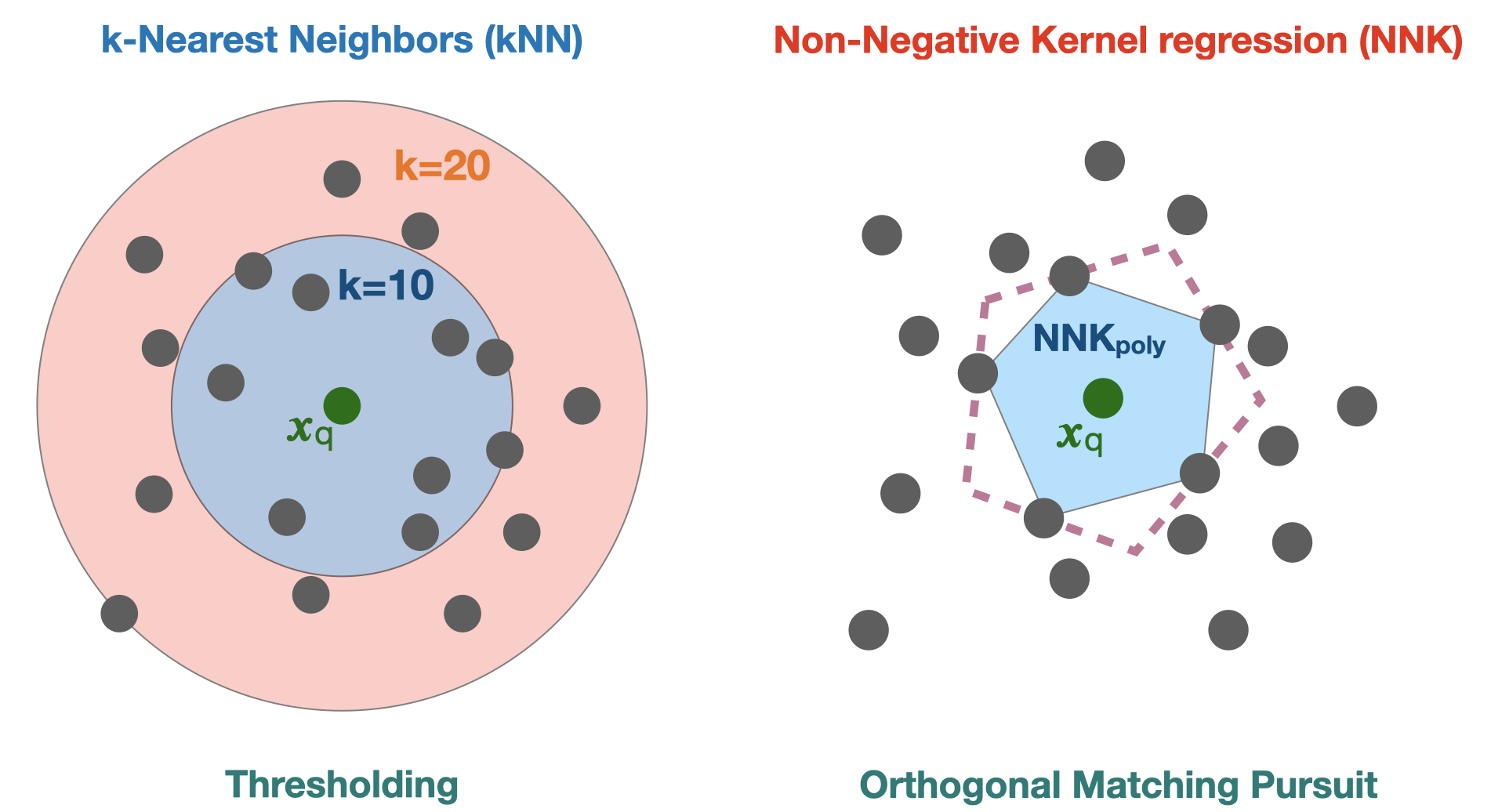
Figure 1: Geometric difference in neighborhood definitions using k-nearest neighbors (kNN) and the proposed NNK approach with a Gaussian kernel. kNN selects neighbors based on the choice of k and can lead to the selection of neighbors that are geometrically redundant, i.e., the vector from the query to neighbors is almost collinear with other vectors joining the query and neighbors. In contrast, the proposed NNK definition selects only neighbors that correspond to non-overlapping directions.

A key contribution of this work is a novel interpretation of the neighborhood definition as a non-negative sparse approximation of the query ${\bm{x}}_{q}$ using data points $\{{\bm{x}}_{1}\dots\bm{x}_{N}\}$. This view of neighborhoods allows one to analyze the problem using tools from sparse signal processing [22] and opens up several directions for further research. In particular, we show that kNN and $\epsilon$-neighborhood are signal approximation based on thresholding, with their corresponding hyperparameters, k and $\epsilon$, used to control the sparsity. Our work is motivated by the well-known limitations of thresholding, which is only optimal when the candidate representation vectors (in our case the neighbors) are orthogonal.

In this work, we leverage the sparse signal representation perspective to (i) establish a new notion of optimality for neighborhood definition and (ii) an improved algorithm, non-negative kernel regression (NNK), based on this optimality criterion. The sparse representation optimality criterion requires approximation errors to be orthogonal to the candidate representation vectors. We show that when applied to our problem this criterion prevents the selection of points that are “geometrically redundant”. This idea is illustrated in Figure 1. Geometrically, the proposed NNK neighborhoods can be viewed as constructing a polytope around the query using points closest to it but eliminating those candidate neighbors that are further away along a similar direction as an already selected neighbor. Thus, instead of selecting the number of neighbors based on pre-set parameters, e.g., k or $\epsilon$, the NNK neighborhood is adaptive to the local data geometry and results in a principled neighbor selection and weight assignment.

1.1 Contributions and organization of the paper

This paper substantially extends our earlier work, a shorter conference publication [23], in two ways.

First, it presents a thorough theoretical analysis of the geometry, sparse representation, and optimization involved in the NNK framework, where we

• further formalize with proofs our geometric characterization of NNK neighbors in input and kernel space via our kernel ratio interval (KRI) theorem (Section 4),

• demonstrate the equivalence between NNK geometry and non-negative basis pursuit algorithms (Section 4.4), and

• make explicit the connection between NNK and previously studied LLE-based neighborhoods [24] and $\ell_{1}$-constrained pursuit methods (Sections 3.3.1,3.4.2);

Second, it offers a comprehensive experimental evaluation of the proposed NNK method in neighborhood and graph-based machine learning problems, where we

• use $70$ OpenML classification datasets to show that NNK neighborhoods produce robust local classifiers outperforming those of kNN, ${\textnormal{k}}^{*}$NN [20] (Section 5.1),

• quantify the scalability and sparsity of NNK graph construction relative to kNN, AEW [25], LLE [24], and Kalofolias [26] graph constructions (Section 5.2.1), and

• validate that NNK graphs lead to better performance in graph-based semi-supervised learning and dimensionality reduction (Sections 5.2.2 and 5.2.3).

In other publications we have used the properties of NNK to revisit and improve methods in image processing [27], data summarization [28], machine learning [29, 30], and geometric evaluation of deep learning models [31, 32, 33]. While these complementary works have reinforced the benefits of NNK, the present work provides the theoretical background and fundamental concepts behind the NNK formulation.

The rest of the paper is organized as follows: Section 2 introduces notations, background, and related work. We discuss the connection between neighborhood definition and basis pursuit for sparse signal approximation in Section 3 and introduce our NNK algorithm in Section 3.3. We then derive the geometrical properties of NNK neighbors in Section 4. We conclude with experimental validation and discussion of the NNK framework in Sections 5 and 6. The proofs for all statements can be found in the Appendix.

2 Background

We start by introducing the notation and two key components, kernel similarity and local linearity of data, that lead to distinct categories of existing neighborhood and graph constructions [34]. We also briefly review related work.

2.1 Notation

Throughout the paper, we use lowercase (e.g., $x$ and $\theta$), lowercase bold (e.g., ${\bm{x}}$ and ${\bm{\theta}}$), and uppercase bold (e.g., ${\bm{M}}$ and ${\bm{\Phi}}$) letters to denote scalars, vectors, and matrices, respectively. We reserve the use of ${\bm{K}}$ for representing the matrix of the kernel function so that the kernel evaluated between two data points $i$ and $j$ is written ${\bm{K}}_{i,j}=\kappa({\bm{x}}_{i},{\bm{x}}_{j})$. Given a subset of indices $S$, ${\bm{x}}_{S}$ denotes the subvector of ${\bm{x}}$ obtained by taking the elements of ${\bm{x}}$ at locations in $S$. A submatrix ${\bm{M}}_{S,S}$ can be obtained similarly from ${\bm{M}}$. The set complement $\bar{S}$ corresponds to the set of indices not in set $S$. We depict the vectors of all zeros and all ones as ${\bm{0}},{\bm{1}}$ respectively. The indicator function is represented using ${\mathbb{I}}:\{\text{False},\text{True}\}\rightarrow\{0,1\}$ and the Hadamard product of matrices is denoted by $\odot$ operator.

A graph ${\mathcal{G}}=({\mathbb{V}},{\mathbb{\xi}})$ is a collection of nodes indexed by the set ${\mathbb{V}}=\{1,\ldots,N\}$ and connected by edges ${\mathbb{\xi}}=\{(i,j,w_{ij})\}$, where $(i,j,w_{ij})$ denotes an edge of weight $w_{ij}\in\mathbb{R}^{+}$ between nodes $i$ and $j$. The weighted adjacency matrix ${\bm{W}}$ of the graph is an $N\times N$ matrix with ${\bm{W}}_{ij}=w_{ij}$. The combinatorial Laplacian of a graph is defined as ${\bm{L}}={\bm{D}}-{\bm{W}}$, where ${\bm{D}}$ is the diagonal degree matrix with ${\bm{D}}_{ii}=\sum_{j}{\bm{W}}_{ij}$. The symmetric normalized Laplacian is defined as ${\mathcal{L}}={\bm{I}}-{\bm{D}}^{-1/2}{\bm{W}}{\bm{D}}^{-1/2}$.

2.2 Similarity kernels

Kernels have a wide range of applications in machine learning [35, 36]. As with most kernel-based works, we focus on kernels satisfying Mercer’s theorem: a kernel function evaluated between two points corresponds to an inner product in a transformed space, the Reproducing Kernel Hilbert space (RKHS)[37, 38], i.e., $\kappa({\bm{x}}_{i},{\bm{x}}_{j})={\bm{\phi}}_{i}^{\top}{\bm{\phi}}_{j}$, where ${\bm{\phi}}_{i},{\bm{\phi}}_{j}$ are the kernel space representations of ${\bm{x}}_{i},{\bm{x}}_{j}$. Similarity kernels are used for assigning weights to selected neighbors in a neighborhood/graph definition. The choice of the kernel is, in general, task- or domain-specific with some predefined kernels widely used in practice. Alternatively, one can also learn a kernel based on available data [39, 40]. Examples of data-driven kernel learning methods for neighborhood definition include [41] and adaptive edge weighting (AEW) [25]. It should be emphasized that the learned kernels in these methods are used with k or $\epsilon$-neighborhood selection and thus only offer a solution for the weight assignment problem.

In this paper we primarily use the Gaussian kernel:

$$\kappa_{\sigma^{2}}({\bm{x}}_{i},{\bm{x}}_{j})=e^{-\frac{\|{\bm{x}}_{i}-{\bm{x}}_{j}\|^{2}}{2\sigma^{2}}},$$ (1)

where $\sigma$ is the bandwidth (variance) of the kernel. We emphasize that the statements and algorithms presented here, unless stated otherwise, are applicable to all symmetric and positive-definite kernels, including those learned from data.

2.3 Locally linear neighborhoods

High-dimensional data is often assumed to lie on or near a smooth manifold and thus can be approximated using locally linear patches. This is the principal assumption behind local linear embedding (LLE) [42], which relies on a local regression objective to approximate a query, i.e.,

$${\bm{\theta}}_{S} =\operatorname*{arg\,min}_{\bm{\theta}}\;\|{\bm{x}}_{q}-{\bm{X}}_{S}{\bm{\theta}}\|^{2}_{{}_{2}},$$ (2)

where ${\bm{X}}_{S}$ is the matrix containing the k-nearest neighbors of ${\bm{x}}_{q}$, whose indices are denoted by set $S$. A solution to (2) can produce both positive and negative values for the entries of ${\bm{\theta}}$, which would be the weights associated with the elements in the set $S$. Thus, [24] reformulated this problem for defining neighborhoods and graphs by introducing non-negativity constraints on the weights.

Subsequent modifications to [24] for neighborhood construction include: post-processing to enforce regularity [43]; formulating a global objective to construct symmetrized graphs [44]; and additional regularizations in the objective to facilitate robust optimization [45, 46]. Alternative approaches such as [26, 47] can be considered as a reformulation of the LLE objective from a graph signal processing perspective with appropriate regularizers.

Table I: Contributions of our proposed method (NNK) in relation to previous works. NNK combines the concepts of non-negativity, kernels, and locally linear neighborhoods. Earlier works did not explore the sparsity or the geometric consequences of non-negativity (why a data point $i$ is selected while another $j$ is not selected for representing a query $q$) in their definitions. The last column demonstrates the geometry of the neighborhood obtained, based on Theorem 1, for Linear and Gaussian kernels (Dataset, Query, Neighbors obtained with non-negative optimization).

2.4 Related work

The proposed NNK framework reduces to non-negativity constrained LLE algorithms under a specific choice of cosine kernel (see Section 3.3.1). We note that kernelized versions of LLE have been previously studied for dimensionality reduction [48, 49], ridge regression [50], subspace clustering [51], and matrix completion [52]. However, we emphasize that these methods did not (1) develop a connection between neighborhood construction and sparse signal approximation, or (2) study the kernelized objective under non-negativity constraints for the purpose of defining neighborhoods. The lack of non-negativity in the kernelized formulations in these related works prevented them from developing geometrical and theoretical properties of their solutions, which are possible for those developed in our framework. We summarize these differences in Table I. To our knowledge, the view of neighborhoods as a sparse signal representation has not been made explicit previously and we believe this perspective can lead to new ideas and even help improve related problems in data analysis. On a different note, works such as [53] solve a complementary problem where the graph is given and kernels based on the graph are constructed for solving machine learning tasks. These methods align with, and reinforce, our intuition that neighborhoods and graphs are structures of similarity defined on a transformed space.

3 Neighborhood definition: A sparse signal approximation view

In this section, we first formulate the neighborhood definition problem as a signal approximation. We then show that the kNN/$\epsilon$-neighborhood methods are equivalent to thresholding-based sparse approximation, and introduce a better representation approach with our NNK framework.

3.1 Problem formulation

Given a dataset of $N$ data points $\{{\bm{x}}_{1},{\bm{x}}_{2},\dots,{\bm{x}}_{N}\}$, the problem of neighborhood definition for a query ${\bm{x}}_{q}$ is that of obtaining a weighted subset of the given $N$ data points that best represents the query. The weights in a neighborhood definition are required to be non-negative, as negative weights would imply a neighbor with negative influence or dissimilarity which are not meaningful in typical neighborhood-based tasks, e.g., density estimation [6] or label propagation [54]. The use of non-negative constraints, either implicitly or explicitly, is a common feature in all neighborhood definitions.

Neighborhood definition for a query can be viewed as a sparse signal approximation problem with non-negative coefficients. The goal is to approximate a signal ${\bm{\phi}}_{q}$ in a kernel space, corresponding to the query ${\bm{x}}_{q}$, as a sparse weighted sum of functions or signals (called atoms) corresponding to the given $N$ data points, i.e.,

$${\bm{\phi}}_{q}\approx{\bm{\Phi}}{\bm{\theta}}$$

where ${\bm{\Phi}}=[{\bm{\phi}}_{1}\;{\bm{\phi}}_{2}\;\dots\;{\bm{\phi}}_{N}]$ is the dictionary of atoms based on the $N$ data points and ${\bm{\theta}}$ is a sparse non-negative vector.

3.2 kNN and $\epsilon$-neighborhood

We first analyze standard approaches such as kNN/$\epsilon$-neighborhood from the signal approximation perspective. A kNN or $\epsilon$-neighborhood approach uses the kernel weights as edge weights. Under the distinction of data and transformed space, a kernel value can be interpreted as the correlation between two data points, i.e., for a query $q$,

$${\bm{\phi}}_{q}^{\top}{\bm{\phi}}_{j}=\kappa({\bm{x}}_{q},{\bm{x}}_{j})={\bm{K}}_{i,j}.$$ (3)

Thus, kNN and equivalently $\epsilon$-neighborhood methods, correspond to a thresholding technique for basis selection wherein atoms corresponding to the k largest correlations are selected from ${\bm{\Phi}}$ to approximate the signal ${\bm{\phi}}_{q}$. This approach is reminiscent of early methods for basis pursuit using thresholding [55], i.e., selecting and weighing atoms based on the magnitude of the correlation between atoms and the signal. This strategy is optimal only when the dictionary is orthogonal (${\bm{\Phi}}^{\top}{\bm{\Phi}}={\bm{I}}$), and is sub-optimal for over-complete or non-orthogonal dictionaries. In our problem setting, the dictionary ${\bm{\Phi}}$ is typically not orthogonal since the atoms (i.e., the neighbors to the query) need not have zero correlation, i.e., in general, ${\bm{\phi}}_{i}^{\top}{\bm{\phi}}_{j}>0$.

3.3 Non-Negative Kernel Regression Neighborhood

We now propose an improved neighborhood definition, non-negative kernel regression (NNK), based on our observation of the sub-optimality (in terms of approximation) of kNN/$\epsilon$-neighborhood. NNK can be viewed as a sparse representation approach where the coefficients ${\bm{\theta}}$ for the representation are such that the error in representation is orthogonal to the space spanned by the selected atoms. We note that this reformulation results in neighborhoods that are adaptive to the local geometry of the data and robust to parameters such as ${\textnormal{k}}/\epsilon$. For a query ${\bm{x}}_{q}$ the NNK weights ${\bm{\theta}}$ are found by solving:

$${\bm{\theta}}_{S}= \operatorname*{arg\,min}_{{\bm{\theta}}\colon{\bm{\theta}}\geq{\bm{0}}}\;\|{\bm{\phi}}_{q}-{\bm{\Phi}}_{S}{\bm{\theta}}\|^{2}_{{}_{2}},$$ (4)

where ${\bm{\Phi}}_{S}$ corresponds to the kernel space representations of an approximate set of data point candidates $S$ for the neighborhood, such as the k nearest neighbors.

Now, employing the kernel trick, given (3) the objective in (4) can be rewritten as the minimization of:

$${\mathcal{J}}_{q}({\bm{\theta}}) =\frac{1}{2}\|{\bm{\phi}}_{q}-{\bm{\Phi}}_{S}{\bm{\theta}}\|^{2}_{{}_{2}}$$

$$=\frac{1}{2}{\bm{\theta}}^{\top}{\bm{K}}_{S,S}{\bm{\theta}}-{\bm{K}}^{\top}_{S,q}{\bm{\theta}}+\frac{1}{2}{\bm{K}}_{q,q}.$$ (5)

Consequently, the NNK neighborhood is obtained as the solution to the optimization problem,

$${\bm{\theta}}_{S} =\operatorname*{arg\,min}_{{\bm{\theta}}\colon{\bm{\theta}}\geq{\bm{0}}}\;\frac{1}{2}{\bm{\theta}}^{\top}{\bm{K}}_{S,S}{\bm{\theta}}-{\bm{K}}^{\top}_{S,q}{\bm{\theta}},$$ (6)

with non-zero elements of the solution ${\bm{\theta}}_{S}$ corresponding to the selected neighbors and weights given by the corresponding values in ${\bm{\theta}}$.

Input : Query ${\bm{x}}_{q}$, Data ${\mathcal{D}}=${${\bm{x}}_{1}\cdots{\bm{x}}_{N}$}, Kernel function $\kappa$, No. of neighbors k

$S$ = {k nearest neighbors of query ${\bm{x}}_{q}$}

${\bm{\theta}}_{S}=\underset{{\bm{\theta}}\geq{\bm{0}}}{\operatorname*{arg\,min}}\;\frac{1}{2}{\bm{\theta}}^{\top}{\bm{K}}_{S,S}{\bm{\theta}}-{\bm{K}}^{\top}_{S,q}{\bm{\theta}}$

$P$ = { elements of $S$ corresponding to ${\mathbb{I}}({\bm{\theta}}_{S}>{\bm{0}})$ }

Output : Neighbors $P$,   Neighbor weights ${\bm{\theta}}_{P}$

Algorithm 1 NNK Neighborhood algorithm

As in other kernel-based learning methods [56], the NNK objective (6) does not require the explicit kernel space representations and needs only knowledge of the similarity, the kernel matrix ${\bm{K}}$, of a subset $S$. The pseudo-code for the proposed method is presented in Algorithm 1.

The NNK framework binds principles that have been key ingredients to neighborhood definitions, namely, kernels and local linearity. Unlike earlier methods which used kernels (predefined or learned) only to define the weights for selected neighbors, the NNK neighborhood can be viewed as identifying a small number of non-negative regression coefficients (as in LLE) for an approximation in the representation space associated with a kernel (see Table I).

3.3.1 NNK and constrained LLE objective

Previously studied LLE [24] is a specific case of the proposed NNK neighborhood algorithm with a kernel similarity defined in the input data space.

Proposition 1.

The NNK algorithm with a query-dependent cosine similarity (7) reduces to the locally linear neighborhood definition.

$$\kappa_{q}({\bm{x}}_{i},{\bm{x}}_{j})=\frac{1}{2}+\frac{({\bm{x}}_{i}-{\bm{x}}_{q})^{\top}({\bm{x}}_{j}-{\bm{x}}_{q})}{2\|{\bm{x}}_{i}-{\bm{x}}_{q}\|\|{\bm{x}}_{j}-{\bm{x}}_{q}\|}$$ (7)

3.4 Basis Pursuits

In this section, we present basis pursuit [57] approaches to sparse signal approximation and their application for defining neighborhoods. We show alongside that the proposed NNK neighborhood is an efficient sparse approximation that leverages the given problem setup, and is equivalent to these pursuit methods under certain conditions.

3.4.1 Matching Pursuits

Matching pursuits (MP) [58] is a greedy algorithm for sparse approximation which iteratively selects atoms that have the highest correlation with the signal’s approximation error at a given iteration. Variants of this method include orthogonal matching pursuits (OMP) [59] and stagewise OMP (Block Selection + OMP) [60], where the coefficients for the selected atoms are recalculated at each step so that the residue is orthogonal to the space spanned by the selected vectors. We now present the steps involved so that MP and OMP can be used in neighborhood definition and then establish the analogy between NNK and OMP.

The first step in MP and OMP is the same, where we find

$$j_{1}=\underset{j}{\operatorname*{arg\,max}}\;{\bm{\phi}}^{\top}_{q}{\bm{\phi}}_{j}={\bm{K}}_{q,j}.$$

With this choice, we can compute the error or residue incurred by approximating ${\bm{\phi}}_{q}$ with a single vector ${\bm{\phi}}_{j_{1}}$ as:

$${\bm{\phi}}_{r_{1}}={\bm{\phi}}_{q}-{\bm{K}}_{q,j_{1}}{\bm{\phi}}_{j_{1}}.$$

Now, at a step $s$, we would find:

$$j_{s}=\operatorname*{arg\,max}_{j\neq j_{1},j_{2}\dots j_{s-1}}\;{\bm{\phi}}^{\top}_{j}{\bm{\phi}}_{r_{s-1}}$$

Then, denote:

$$\quad{\bm{\Phi}}_{S}=\left[{\bm{\phi}}_{j_{1}}\;{\bm{\phi}}_{j_{2}}\;\dots\;{\bm{\phi}}_{j_{s}}\right],$$

where the $S=\{j_{1},\;\ldots\;j_{s}\}$ are the indices of all the selected atoms so far for representation. In MP, one assigns the correlation between the residue and the selected atom as weights for approximation. However, in OMP, we need to find weights ${\bm{w}}_{S}$ associated with each selected basis such that the energy of the residue is minimized, i.e.,

$${\bm{w}}_{S} =\underset{{\bm{w}}\colon{\bm{w}}\geq{\bm{0}}}{\operatorname*{arg\,min}}\;\|{\bm{\phi}}_{r_{S}}\|^{2}$$

$$=\underset{{\bm{w}}\colon{\bm{w}}\geq{\bm{0}}}{\operatorname*{arg\,min}}\;{\bm{K}}_{q,q}-2{\bm{K}}_{S,q}^{\top}{\bm{w}}_{S}+{\bm{w}}_{S}^{\top}{\bm{K}}_{S,S}{\bm{w}}_{S},$$ (8)

where ${\bm{\phi}}_{r_{S}}={\bm{\phi}}_{q}-{\bm{\Phi}}_{S}{\bm{w}}_{S}$ is the residue at step $s$. This ensures that the approximation error is orthogonal to the span of the selected atoms ${\bm{\Phi}}_{S}$.

Note that by constraining the weights to be positive, the span of selected bases at each step is a convex cone, while the residue is orthogonal to this cone [61]. We see that solving for the weights ${\bm{w}}_{S}$ in (8) is equivalent to the NNK objective (6) given the set $S$. Thus, the proposed NNK algorithm (Algorithm 1) bypasses the greedy selection with a pre-selected set of good atoms avoiding expensive computation (iterative selection and orthogonalization). We note that given a set of pre-selected atoms it is straightforward to perform an orthogonal projection, such as the one performed at each OMP step. Our problem makes it possible to perform this pre-selection using computationally efficient approximate neighborhood methods. Thus, we do not need to perform greedy selection and instead can use an approximate neighborhood method to choose the set $S$ without loss in performance, as long as $S$ is large enough (so that all candidates needed to form an optimal neighborhood are likely to be included). Algorithm 2 provides the pseudo-code for neighborhood definition based on MP and OMP with sequential neighbors selection.

Input : Query ${\bm{x}}_{q}$, Data ${\mathcal{D}}=${${\bm{x}}_{1}\cdots{\bm{x}}_{N}$}, Kernel function $\kappa$, Maximum no. of neighbors k

$j_{1}=\operatorname*{arg\,max}_{j}\;{\bm{K}}_{q,j}$

${\bm{\theta}}_{1}={\bm{K}}_{q,j_{1}},\quad S=\{j_{1}\}$

for  $s=2,3,\dots\textnormal{k}$  do

      $j_{s}=\underset{j\notin S}{\operatorname*{arg\,max}}\;{\bm{K}}_{q,j}-{\bm{K}}^{\top}_{S,j}{\bm{\theta}}_{s-1}$

      if  ${\bm{K}}_{q,j_{s}}-{\bm{K}}^{\top}_{S,j_{s}}{\bm{\theta}}_{s-1}<0$  then

          break

           if  OMP  then

               ${\bm{\theta}}_{s}=\underset{{\bm{\theta}}\geq{\bm{0}}}{\operatorname*{arg\,min}}\;\frac{1}{2}{\bm{\theta}}^{\top}{\bm{K}}_{S,S}{\bm{\theta}}-{\bm{K}}^{\top}_{S,q}{\bm{\theta}}$

                else

                    ${\bm{\theta}}^{\top}_{s}=\left[{\bm{\theta}}_{s-1}^{\top}\;\;({\bm{K}}_{q,j_{s}}-{\bm{K}}^{\top}_{S,j_{s}}{\bm{\theta}}_{s-1})\right]$

                     $S=S\cup\{j_{s}\}$

                    

                     end for

                    Output : Neighbors $S$,   Neighbor weights ${\bm{\theta}}_{S}$

Algorithm 2 MP and OMP Neighborhood algorithms

3.4.2 $l_{1}$ regularized pursuits

Another set of methods for solving sparse approximation problems involves a convex relation where one softens the sparsity constrain ($l_{0}$ norm of reconstruction coefficients) with an $l_{1}$ norm constrain [62, 63]. These approaches, also known as least absolute shrinkage and selection operator (LASSO) regression [64], allow for the use of optimization techniques such as linear programming to obtain an approximate sparse solution. A neighborhood definition at a query $q$ using a $l_{1}$ regularized basis pursuit corresponds to an optimization problem of the form

$${\bm{\theta}}_{{\mathcal{D}}} =\operatorname*{arg\,min}_{{\bm{\theta}}\colon{\bm{\theta}}\geq{\bm{0}}}\;\frac{1}{2}{\bm{\theta}}^{\top}{\bm{K}}_{{\mathcal{D}},{\mathcal{D}}}{\bm{\theta}}-{\bm{K}}^{\top}_{{\mathcal{D}},q}{\bm{\theta}}+\eta\|{\bm{\theta}}\|_{1},$$

where ${\mathcal{D}}$ is the set of all $N$ data points and $\eta$ is the Lagrangian hyperparameter. Given the non-negativity constraint on the coefficients in our setting, we can replace the $l_{1}$ norm by the sum, leading to:

$${\bm{\theta}}_{{\mathcal{D}}} =\operatorname*{arg\,min}_{{\bm{\theta}}\colon{\bm{\theta}}\geq{\bm{0}}}\;\frac{1}{2}{\bm{\theta}}^{\top}{\bm{K}}_{{\mathcal{D}},{\mathcal{D}}}{\bm{\theta}}-{\bm{K}}^{\top}_{{\mathcal{D}},q}{\bm{\theta}}+\eta{\bm{\theta}}^{\top}{\bm{1}}.$$ (9)

Proposition 2.

Let ${\bm{\theta}}^{*}$ be the solution to objective (9). Then,

$$\forall j\colon{\bm{K}}_{q,j}<\eta\qquad{\bm{\theta}}^{*}_{j}=0$$ (10)

Proposition 2 implies that the set $\bar{S}=\{i\colon{\bm{K}}_{q,i}<\eta\}$ can be safely removed from the optimization since ${\bm{\theta}}^{*}_{\bar{S}}=0$. Thus objective (9) is equivalent to the NNK objective (6) with set $S$, such that ${\mathcal{D}}=S\cup\bar{S}$ and $S\cap\bar{S}=\emptyset$, i.e., $S$ is the set of data points with similarity greater than $\eta$. Thus, choosing $S$ as a set of kNN neighbors to initialize the objective (6) provides an optimal solution to (9) with parameter $\eta$.

3.5 Graph construction

The NNK neighborhood definition in Section 3.3 and alternative basis pursuit approaches in Section 3.4 can be adapted for graph construction by solving for the neighborhood at each data point ${\bm{x}}_{i}$ to first obtain a directed graph adjacency matrix ${\bm{W}}$, namely, ${\bm{W}}_{S,i}={\bm{\theta}}_{S}$ and ${\bm{W}}_{\bar{S},i}={\bm{0}}$. To obtain an undirected graph, we observe that an edge conflict may occur, say between nodes $i$ and $j$, due to the difference in the local neighborhood of the nodes, i.e., the influence of $i$ on $j$ depends on the neighborhood of $j$ and vice versa. In such a scenario, we consider the approximation error corresponding to nodes $i$ and $j$, namely ${\mathcal{J}}_{i}({\bm{\theta}})$ and ${\mathcal{J}}_{j}({\bm{\theta}})$ from (5), and keep the weight $w_{ij}$ corresponding to the smallest of the two objectives (i.e., $q=i$ and $q=j$). We note that the proposed symmetrization, though intuitive from a representation perspective, requires further study and we leave its formulation and connection to downstream performance as open problems for future work. Algorithm 3 provides the pseudo-code for NNK graph construction.

Input : Data ${\mathcal{D}}=$ {${\bm{x}}_{1}\cdots{\bm{x}}_{N}$}, Kernel function $\kappa$, No. of neighbors k

for  $i=1,2,\dots N$  do

      $S=$ { k nearest neighbors of ${\bm{x}}_{i}$ in ${\mathcal{D}}_{-i}$}

      ${\bm{\theta}}_{S}=\underset{{\bm{\theta}}\geq{\bm{0}}}{\operatorname*{arg\,min}}\;\frac{1}{2}{\bm{\theta}}^{\top}{\bm{K}}_{S,S}{\bm{\theta}}-{\bm{K}}^{\top}_{S,i}{\bm{\theta}}$

      ${\mathcal{J}}_{i}=\frac{1}{2}{\bm{\theta}}^{\top}_{S}{\bm{K}}_{S,S}{\bm{\theta}}_{S}-{\bm{K}}^{\top}_{S,i}{\bm{\theta}}_{S}+\frac{1}{2}{\bm{K}}_{i,i}$

      ${\bm{W}}_{S,i}={\bm{\theta}}_{S},\;\;{\bm{W}}_{\bar{S},i}=\mathbf{0}$

      ${\bm{E}}_{S,i}={\mathcal{J}}_{i}\>{\bm{1}},\;\;{\bm{E}}_{\bar{S},i}=\mathbf{0}$

     

      end for

     ${\bm{W}}={\mathbb{I}}({\bm{E}}\leq{\bm{E}}^{\top})\odot{\bm{W}}+{\mathbb{I}}({\bm{E}}>{\bm{E}}^{\top})\odot{\bm{W}}^{\top}$

      Output : Graph Adjacency ${\bm{W}}$,   Local error ${\bm{E}}$

Algorithm 3 NNK Graph algorithm

3.6 Complexity

The proposed NNK method consists of two steps. First, we find k-nearest neighbors corresponding to each node. Although brute force implementation has complexity $O(N{\textnormal{k}}d)$, there exist efficient algorithms to find approximate neighborhoods using sub-linear-time search with additional memory [65]. Second, a non-negative kernel regression (6) is solved at each node. This objective is a constrained quadratic function of ${\bm{\theta}}$ and can be solved efficiently using structured programming methods that require $O({\textnormal{k}}^{3})$ or, with more careful analysis, $O({\textnormal{k}}\hat{{\textnormal{k}}}^{2})$ complexity, where $\hat{{\textnormal{k}}}$ is the number of neighbors with non-zero weights in the optimal solution. In summary, the NNK framework defines a neighborhood with an initialization based on kNN followed by a weight estimation with a runtime complexity that is, at most, cubic in the size of the initial neighborhood set $S$.

In practice, as observed in our experiments (Section 5), the added complexity of NNK, after initializing with kNN, is often negligible compared to the cost of kNN, given that $Nd>>{\textnormal{k}}^{2}$. We note that the choice of k for the initial set $S$ provides a trade-off between runtime complexity and optimality: a small k has lower complexity but results in a set $S$ that is not representative enough, while a larger k has higher complexity but allows for obtaining the optimal neighborhood. For the graph construction problem, the runtime of the NNK optimization is $O(N{\textnormal{k}}\hat{{\textnormal{k}}}^{2})$, in addition to the time required for kNN. Note that, due to the local nature of the optimization problem, the NNK algorithm can be executed in parallel and is typically limited by the complexity of finding a good set of initial neighbors.

4 Geometric Interpretation

Unlike existing neighborhood definitions, such as kNN, where a neighbor selection for a query $q$ involving two points $i$ and $j$ is driven solely based on the metric on $(q,i)$ and $(q,j)$, NNK also takes into account the relative positions of nodes $i$ and $j$ using the metric on $(i,j)$. We now present a theoretical analysis of the geometry in NNK neighborhoods.

4.1 NNK and active constraint set condition

In constrained optimization problems, some constraints will be strongly binding, i.e., the solution at some indices will be zero to satisfy the KKT condition of optimality (outlined in Section B.1). These constraints are referred to as active constraints, knowledge of which helps reduce the problem for optimization and analysis using only the inactive subset. This is because any constraints that are active at a current feasible solution will remain active at the optimum [66].

Proposition 3.

The NNK optimization objective (5) at a query ${\bm{x}}_{q}$ satisfies active constraint conditions. Given a partition set $P$ such that ${\bm{\theta}}_{P}>0$ (inactive) and ${\bm{\theta}}_{\bar{P}}=0$ (active), the solution $[{\bm{\theta}}_{P}\;{\bm{\theta}}_{\bar{P}}]^{\top}$ is the optimal solution to NNK iff

$${\bm{K}}_{P,P}{\bm{\theta}}_{P} ={\bm{K}}_{P,q}$$ (11)

$${\bm{K}}^{\top}_{P,\bar{P}}{\bm{\theta}}_{P}-{\bm{K}}_{\bar{P},q} \geq{\bm{0}}$$ (12)

Proposition 3 allows us to analyze the neighbors obtained in the NNK framework, one pair at a time, as a data point that is zero weighted (active constraint) will remain zero weighted at the optimal solution. We first introduce conditions for the existence of NNK neighbors in the form of the Kernel Ratio Interval (KRI) theorem, which is applied inductively to unfold the geometry of NNK neighborhoods.

4.2 Geometry of NNK neighbors

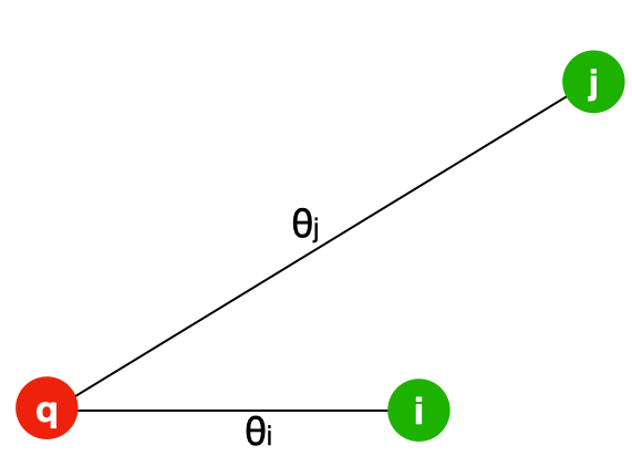
Figure 2: Problem setup for a query $q$ with two points $i,j$.

Theorem 1.

Kernel Ratio Interval: Given a scenario with a query $q$ and two data points, $i$ and $j$ (see Fig 2) and a similarity kernel with range $[0,1]$, the necessary and sufficient condition for both $i$ and $j$ to be chosen as neighbors of $q$ by NNK is given by

$${\bm{K}}_{i,j}<\frac{{\bm{K}}_{q,i}}{{\bm{K}}_{q,j}}<\frac{1}{{\bm{K}}_{i,j}}.$$ (13)

In words, Theorem 1 states that when $i$ and $j$ are very similar, it is less likely that both will be chosen as neighbors of $q$, because the interval in (13), which defines when this can happen, becomes narrower. The KRI condition of (13) does not make any assumptions on the kernel, other than that it be symmetric with values in $[0,1]$.

Corollary 1.1.

Plane Property: Each NNK neighbor corresponds to a hyperplane with normal in the direction of the line joining the neighbor and query (Figure 3(a)), points beyond which will not be NNK neighbors for the case of Gaussian kernel (1).

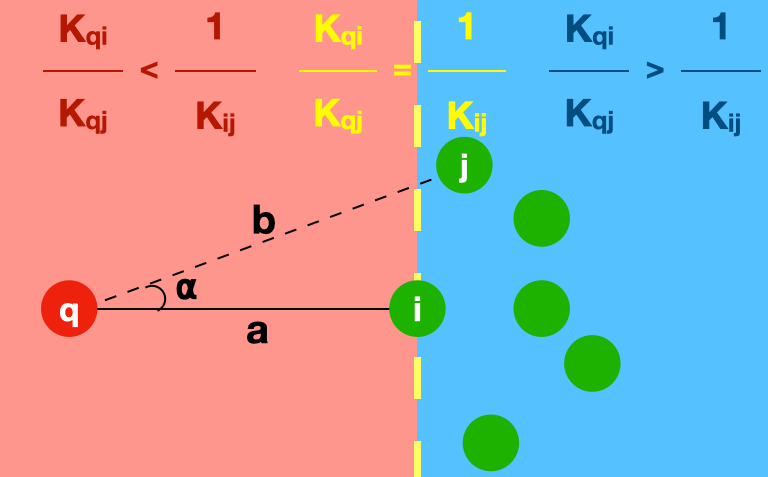
(a)

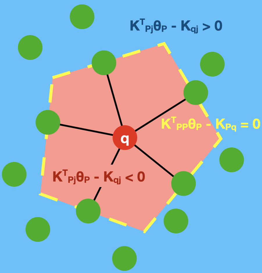
(b)

Figure 3: Local geometry (denoted in red) of NNK neighborhood for a kernel similarity proportional to the distance between the data points. (a) Hyper plane associated with a selected NNK neighbor. (b) Convex polytope corresponding to NNK neighbors around a query.

Corollary 1.1 can be described in terms of projections as illustrated in Figure 3(a). Assume that query $q$ is connected to a neighbor $i$ ($\theta_{i}>0$). Now, define a hyperplane that contains $i$ and is perpendicular to the line going from $q$ to $i$. Then any data point $j$ that is beyond this hyperplane (i.e., on the half space not containing $q$) will not be an NNK neighbor ($\theta_{j}=0$). This is because the orthogonal projection of (${\bm{x}}_{j}-{\bm{x}}_{q}$) along the direction (${\bm{x}}_{i}-{\bm{x}}_{q}$) is at a position beyond ${\bm{x}}_{i}$.

Corollary 1.2.

Polytope Property (Local geometry of NNK): The local geometry of the NNK neighborhood with Gaussian kernel (1), for a given query $q$, is a convex polytope around the query (Figure 3(b)). The optimal solution to the NNK objective (6) with ${\bm{\theta}}=[{\bm{\theta}}_{P},\;{\bm{\theta}}_{\bar{P}}]^{\top}$, where ${\bm{\theta}}_{P}>0$ and ${\bm{\theta}}_{\bar{P}}=0$ satisfies

1. ${\bm{K}}^{\top}_{P,j}{\bm{\theta}}_{P}-{\bm{K}}_{q,j}\geq 0$ $\quad\iff\;\exists\;i\;\in\;P\;\colon\;\frac{{\bm{K}}_{q,i}}{{\bm{K}}_{q,j}}\geq\frac{1}{{\bm{K}}_{i,j}}$

2. ${\bm{K}}^{\top}_{P,j}{\bm{\theta}}_{P}-{\bm{K}}_{q,j}<0$ $\quad\iff\;\forall\;i\;\in\;P\;\colon\;\frac{{\bm{K}}_{q,i}}{{\bm{K}}_{q,j}}<\frac{1}{{\bm{K}}_{i,j}}$

The conditions in Corollary 1.2 are a direct consequence of applying Corollary 1.1 to a series of points. Gathering successive conditions leads to forming a polytope, as illustrated in Fig. 3(b), and to the optimality conditions of the active set Proposition 3. In other words, the NNK neighborhood algorithm constructs a polytope around a query using selected neighbors while disconnecting geometrically redundant data points outside the polytope. This suggests that the local connectivity of NNK neighbors is a function of the local dimension of the data manifold [67].

We note that corollaries 1.1 and 1.2 are applicable to all kernels that are monotonic with respect to the distance between data points. However, we emphasize that equivalent geometric conditions based on the KRI can be obtained for other kernels. For example, in the case of linear kernels, it can be shown that the NNK geometry obtained is that of a convex cone with each selected neighbor corresponding to a hyperplane passing through the origin [61] (see Figure I).

4.3 NNK Geometry in kernel space

In some cases, such as bio-sequences or text documents, for which it may be difficult to represent the input as explicit feature vectors, using a distance-based kernel, such as the Gaussian kernel in (1), is not feasible, and alternative kernel similarity measures need to be employed [68]. However, the RKHS space associated with these alternative kernels still possesses an inner product and norm. Thus, it is valuable to consider the geometry of the kernel space to understand neighborhood algorithms, even when the input space geometry is not explainable. To this end, we now derive properties of NNK neighborhoods in terms of the distances and angles between the RKHS mappings of the input data.

Proposition 4.

Points in an RKHS associated with any kernel function $\kappa$ with range in $[0,1]$ are characterized by an RKHS distance given by,

$$\tilde{d}^{2}(i,j)=\|{\bm{\phi}}_{i}-{\bm{\phi}}_{j}\|^{2}=2-2\kappa({\bm{x}}_{i},{\bm{x}}_{j}).$$ (14)

Theorem 2.

Given distance (14), the necessary and sufficient condition for two points $i,j$ to be NNK neighbors to a query $q$ is

$$\theta_{i}\neq 0\iff \tilde{d}^{2}(q,j)+\tilde{d}^{2}(i,j)-\tilde{d}^{2}(q,i)>\frac{\tilde{d}^{2}(q,j)\tilde{d}^{2}(i,j)}{2}$$

$$\theta_{j}\neq 0\iff \tilde{d}^{2}(q,i)+\tilde{d}^{2}(i,j)-\tilde{d}^{2}(q,j)>\frac{\tilde{d}^{2}(q,i)\tilde{d}^{2}(i,j)}{2}$$

Corollary 2.1.

Using the law of cosines,

$$\theta_{i}\neq 0\iff\cos\alpha>\frac{\tilde{d}(q,j)\tilde{d}(i,j)}{4}$$ (15)

$$\theta_{j}\neq 0\iff\cos\beta>\frac{\tilde{d}(q,i)\tilde{d}(i,j)}{4}$$ (16)

where $\alpha,\beta$ are the angles subtended by the chords joining ($\phi_{i},\phi_{j}$) and ($\phi_{q},\phi_{j}$), ($\phi_{q},\phi_{i}$) respectively as in Figure 4(a).

Corollary 2.1 allows us to provide a bound for the angle subtended and the length of chords for an NNK neighbor, namely,

$$\theta_{i}\neq 0\iff\frac{\pi}{3}<\alpha<-\frac{\pi}{3}$$ (17)

where we use the fact that the RKHS distance (14) is is upper bounded by $2$. A similar result holds for $j$ and $\beta$.

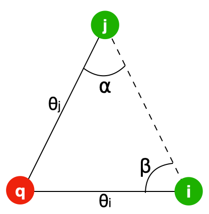
(a)

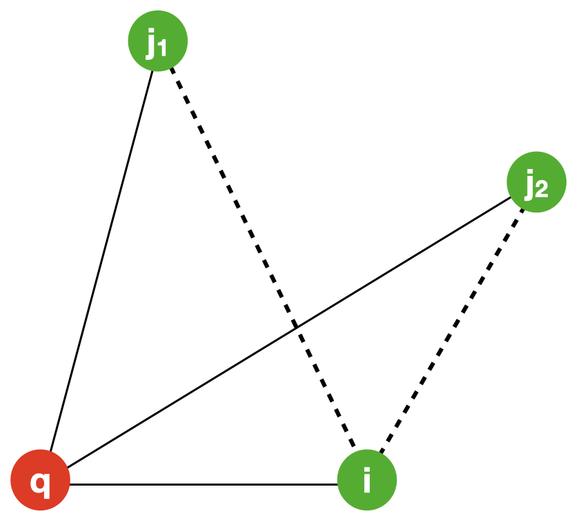
(b)

Figure 4: (a) Geometric setup of NNK in RKHS. (b) Problem setup at the $2^{nd}$ step of pursuit in MP, OMP neighborhoods.

4.4 Geometry of MP, OMP neighborhoods

We now show that Theorem 1 can also be applied to matching pursuits-based neighborhood definitions. We note that the results in this section are applicable to other problems with non-negative basis pursuits [69, 70]. The geometric conditions presented here provide a potential approach to efficiently screen and select atoms in iterative basis pursuits for non-negative approximations with large dictionaries.

Assume atom ${\bm{\phi}}_{i}$ is selected in the first step of either the MP or the OMP algorithm (Algorithm 2). Then, the approximation residue is given by ${\bm{\phi}}_{r_{1}}={\bm{\phi}}_{q}-{\bm{K}}_{q,i}{\bm{\phi}}_{i}$.

Now, observe that

$${\bm{\phi}}^{\top}_{r_{1}}{\bm{\phi}}_{q} =1-{\bm{K}}^{2}_{q,i}\geq 0\quad\text{and}$$ (18)

$${\bm{\phi}}^{\top}_{r_{1}}{\bm{\phi}}_{i} ={\bm{K}}_{q,i}-{\bm{K}}_{q,i}{\bm{K}}_{i,i}=0,\quad\text{since }{\bm{K}}_{i,i}=1.$$ (19)

Equation (18) shows that the residue at the end of the first step can only be exactly zero iff ${\bm{K}}_{q,i}=1$. However, the residue at the end of the first step is orthogonal to the selected atom (${\bm{\phi}}_{i}$) as shown in (19).

For the second step of the algorithm, consider two points $j_{1}$ and $j_{2}$ as in Fig. 4(b). By Theorem 1, we expect $j_{2}$ to be not selected and $j_{1}$ to be selected. The equations below show that the pursuit algorithms carry out a selection process where points that do not satisfy the KRI conditions are indeed not selected for representation.

$${\bm{\phi}}^{\top}_{r_{1}}{\bm{\phi}}_{j_{2}}={\bm{K}}_{q,j_{2}}-{\bm{K}}_{q,i}{\bm{K}}_{i,j_{2}} \leq 0 \iff\frac{{\bm{K}}_{q,i}}{{\bm{K}}_{q,j_{1}}}\geq\frac{1}{{\bm{K}}_{i,j_{1}}}$$

$${\bm{\phi}}^{\top}_{r_{1}}{\bm{\phi}}_{j_{1}}={\bm{K}}_{q,j_{1}}-{\bm{K}}_{q,i}{\bm{K}}_{i,j_{1}} >0 \iff\frac{{\bm{K}}_{q,i}}{{\bm{K}}_{q,j_{1}}}<\frac{1}{{\bm{K}}_{i,j_{1}}}$$

The weights after selection for the set $S=\{i,j_{1}\}$ in the case of MP is given by ${\bm{\theta}}^{(MP)}_{S}=\left[{\bm{K}}_{q,i}\;{\bm{K}}_{q,j_{1}}-{\bm{K}}_{q,i}{\bm{K}}_{i,j_{1}}\right]^{\top}$, while in OMP, ${\bm{\theta}}^{(OMP)}_{S}$ is computed by minimizing (6). In MP, the updated residue is orthogonal only to the last selected data point $j_{1}$,

$${\bm{\phi}}^{(MP)\top}_{r_{2}}{\bm{\phi}}_{i}= {\bm{K}}_{q,i}-{\bm{K}}_{q,i}{\bm{K}}_{i,i}-({\bm{K}}_{q,j_{1}}-{\bm{K}}_{q,j_{1}}{\bm{K}}_{i,j_{1}}){\bm{K}}_{i,j_{1}}$$

$$= -({\bm{K}}_{q,j_{1}}-{\bm{K}}_{q,j_{1}}{\bm{K}}_{i,j_{1}}){\bm{K}}_{i,j_{1}}\neq 0$$ (20)

$${\bm{\phi}}^{(MP)\top}_{r_{2}}{\bm{\phi}}_{j_{1}}= {\bm{K}}_{q,j_{1}}-{\bm{K}}_{q,i}{\bm{K}}_{i,j_{1}}-({\bm{K}}_{q,j_{1}}-{\bm{K}}_{q,j_{1}}{\bm{K}}_{i,j_{1}})$$

$$= 0$$ (21)

while in OMP, the residue is orthogonal to all selected atoms as guaranteed by the first-order optimality condition of the objective (6), i.e, ${\bm{K}}_{S,S}{\bm{\theta}}^{(OMP)}-{\bm{K}}_{S,q}=0$.

$${\bm{\phi}}^{(OMP)\top}_{r_{2}}{\bm{\phi}}_{i}= {\bm{K}}_{q,i}-{\bm{\theta}}^{(OMP)\top}_{S}{\bm{K}}_{S,i}=0$$ (22)

$${\bm{\phi}}^{(OMP)\top}_{r_{2}}{\bm{\phi}}_{j_{1}}= {\bm{K}}_{q,j_{1}}-{\bm{\theta}}^{(OMP)\top}_{S}{\bm{K}}_{S,j_{1}}=0$$ (23)

This scenario repeats in the subsequent pursuit steps where selected neighbors in MP are orthogonal only to the last neighbor selected, while in OMP to all selected neighbors. The iterative selection ends when the maximum number of allowed neighbors is reached or when no positively correlated atom is available for representing the residue i.e,

$$\forall m\notin S\quad{\bm{K}}_{q,m}-{\bm{\theta}}_{S}{\bm{K}}_{S,m}\leq 0$$

The above criteria prevent pursuit algorithms from selecting points that do not contribute to the non-negative approximation as these correspond to points outside the polytope (Corollary 1.2). Note that, unlike unconstrained pursuit where adding more atoms often leads to a better approximation, increasing the number of selected atoms does not necessarily correspond to better representation in non-negative pursuit [70].

5 Experiments and Results

We demonstrate the benefits of the proposed NNK framework in neighborhood-based classification, graph-based label propagation and dimensionality reduction. Code for experiments is available at https://github.com/STAC-USC/.

5.1 NNK neighborhood

We study the proposed NNK neighborhood for classification (binary and multi-class) using a plug-in classifier ${\mathbb{I}}(\hat{f}({\bm{x}}_{q})>0)$ based on the neighborhood estimate

$$\hat{f}({\bm{x}}_{q})=\sum_{i\in{\mathcal{N}}({\bm{x}}_{q})}\frac{\theta_{i}}{\sum_{j\in{\mathcal{N}}({\bm{x}}_{q})}\theta_{j}}\;y_{i},$$ (24)

where ${\mathcal{N}}({\bm{x}}_{q})$ is the neighborhood defined for query ${\bm{x}}_{q}$ and $\theta_{i},y_{i}$ are the vector of weights and the one-hot encoded label associated with ${\bm{x}}_{i}$, respectively.

Experiment setup: We compare the NNK neighborhood against two baselines, the standard weighted kNN and an adaptive neighborhood approach ${\textnormal{k}}^{*}$NN [20]. We make use of the Gaussian kernel (1) for neighborhoods defined with kNN and NNK. Two groups of datasets are considered: $(i)$ AR face [71], Extended YaleB [72], Isolet, and USPS [73] with their standard train/test split, and $(ii)$ $70$ datasets from OpenML [74]. The OpenML datasets are obtained based on the number of dimensions ($d\in[20,1000]$), the number of samples ($N\in[1000,20000]$), with no restriction on the number of classes as in [75]. All datasets are standardized using the empirical mean and variance estimated with training data. We repeat all experiments $10$ times and report average performances and ablation studies.

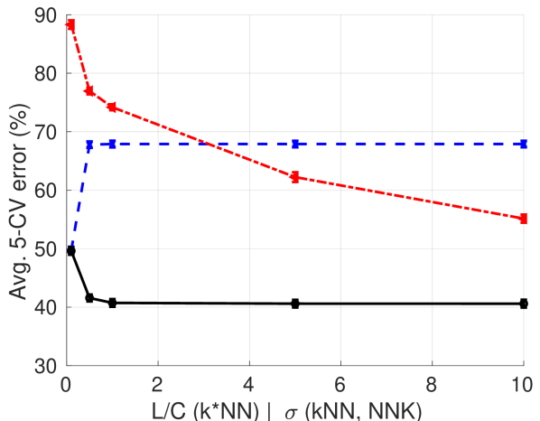
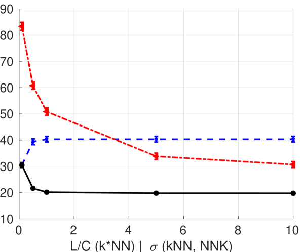
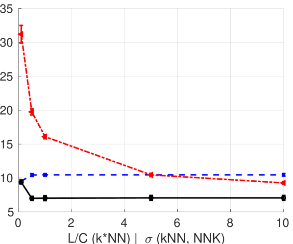
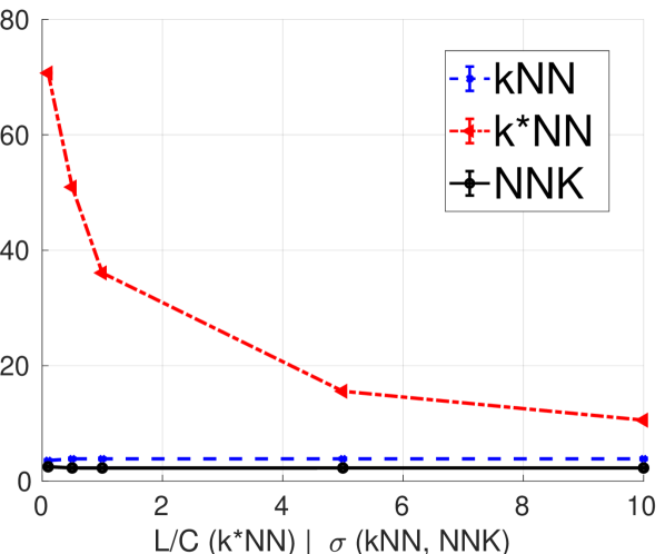
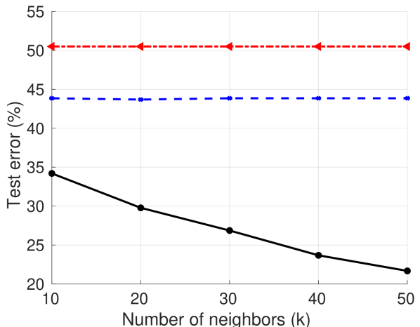
(a) AR Face

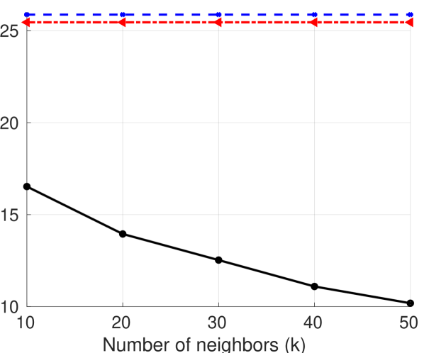
(b) YaleB Face

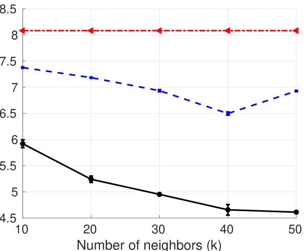
(c) Isolet

(d) USPS

Figure 5: Top: Average cross-validation error for different values of hyperparameters associated with ${\textnormal{k}}^{*}$NN , kNN, and NNK. The value of k in kNN and NNK is set to $10$ in these experiments. Bottom: Test error of kNN and NNK for different values of k with hyperparameter $\sigma$ selected using cross-validation. Here we include ${\textnormal{k}}^{*}$NN for reference. We see that NNK, unlike kNN and ${\textnormal{k}}^{*}$NN, produces better performance for a wide range of hyperparameter values.

AR, YaleB, Isolet, USPS: We use these datasets to perform ablation and $5$-fold cross-validation studies on parameters ${\textnormal{k}},\sigma$ used in kNN and NNK, and $L/C$ value in ${\textnormal{k}}^{*}$NN. We consider values ${\textnormal{k}}\in\{10,20,30,40,50\}$ and $\sigma,L/C$ in $\{0.1,0.5,1,5,10\}$ as in [20].

Dataset	$N_{tr},N_{te}$	$d$	$N_{class}$	kNN	${\textnormal{k}}^{*}$NN	NNK
AR	$2000,600$	$540$	$100$	$43.68$	$50.5$	$\mathbf{21.68}$
YaleB	$1216,1198$	$504$	$38$	$25.88$	$25.46$	$\mathbf{10.18}$
Isolet	$6238,1559$	$617$	$26$	$6.50$	$8.08$	$\mathbf{4.61}$
USPS	$7291,2007$	$256$	$10$	$6.33$	$13.45$	$\mathbf{4.49}$

Table II: Test classification error (in $\%$, lower is better) using local neighborhood methods on datasets with train ($N_{tr}$) and test ($N_{te}$) sample size, dimension ($d$), and classes ($N_{class}$). NNK-based classification consistently outperforms baseline methods while being robust to choices of ${\textnormal{k}},\sigma$.

Table II presents the classification performance on the test datasets with different neighborhood classifiers using training data. Reported performance corresponds to the best set of hyperparameters (obtained with cross-validation) for each method and demonstrates the gains of NNK relative to the two baselines.

Figure 5 shows the cross-validation and test classification performance for various parameter choices. We note that both kNN and NNK are less affected by the hyperparameter $\sigma$ relative to ${\textnormal{k}}^{*}$NN, which is heavily influenced by the choice of $L/C$. In particular, we see that there exists a narrow choice of $\sigma$ where kNN achieves maximum performance, as larger $\sigma$ leads to higher weights assigned to farther away neighbors. In contrast, the NNK algorithm produces a robust performance for a broad range of $\sigma$. Further, it can be seen that NNK estimates saturate with increasing k. The stability in NNK estimation is due to the fact that each neighbor is selected only if it belongs to a new direction in space not previously represented. Note that NNK estimation outperforms kNN and ${\textnormal{k}}^{*}$NN, in these datasets, even for a sub-optimal choice of the kernel parameter $\sigma$ and the number of neighbors k.

OpenML datasets: The train/test split for each dataset is obtained by randomly dividing the data into two equal halves with hyperparameters $\sigma$ or $L/C$ obtained via cross-validation as in the previous set of experiments. The value of k in kNN and NNK is fixed to $30$.

Method	Avg. error ($\%$)	Wins/Ties/Losses	Avg. Rank
kNN	18.06 (0.83)	7/24/39	2.0571
${\textnormal{k}}^{*}$NN	20.71 (1.04)	19/10/50	2.2714
NNK	16.26 (0.74)	44/9/17	1.6714

Table III: Performance summary of neighborhood methods on $70$ OpenML datasets. Listed metrics include (i) Average classification error and standard deviation (in parentheses) across all datasets, (ii) the number of datasets where a method performs better than the other two (Win), performs within one standard deviation of the best performance (Tie), and performs poorly in comparison (Loss), and (iii) average rank of the method based on the classification ($1^{st},2^{nd},3^{rd}$).

Table III provides a summary of the classification performance on all $70$ datasets. We observe that NNK achieves better overall performance in comparison to baselines. ${\textnormal{k}}^{*}$NN, though successful in some cases, falls short in several datasets, which is indicative of its inability to adapt to varied dataset scenarios. In contrast, NNK demonstrates flexibility to feature and class disparities in several datasets. The failure cases of NNK, such as the binarized version of regression designed in [76] ($11$ of $17$ losses), correspond to datasets with non-informative feature dimensions containing only noise. In such scenarios, redundancy in the representation, as in kNN, can provide a better estimate. We leave this NNK limitation for future study.

5.2 NNK graphs

In this section, we compare NNK graphs (Algorithm 3) and the basis pursuit variants (MP, OMP from Algorithm 2) with graph construction methods based on weighted kNN, LLE [24], AEW [25], and the method by Kalofolias [26]. We measure the goodness of the graphs in terms of the sparsity of the graphs, runtime required for graph construction, and performance on downstream tasks. As in neighborhood experiments, we use the Gaussian kernel defined in (1). We set $\sigma$ parameter such that the kNN approach is able to assign a nonzero weight to all its k neighbors, i.e. a connected graph, by ensuring the ${\textnormal{k}}^{th}$ neighbor distance is within $3*\sigma$. For a fair comparison, we use the same $\sigma$ value for AEW, MP, OMP, and NNK graph constructions.

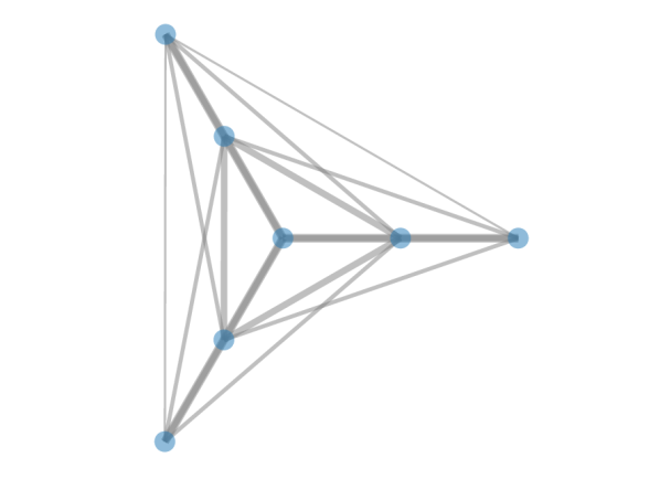
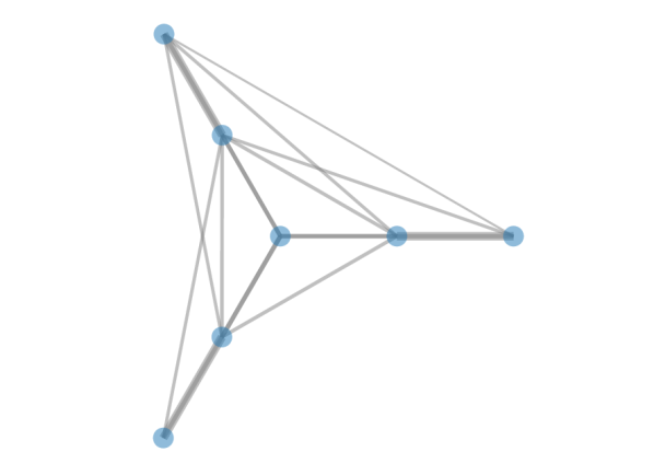
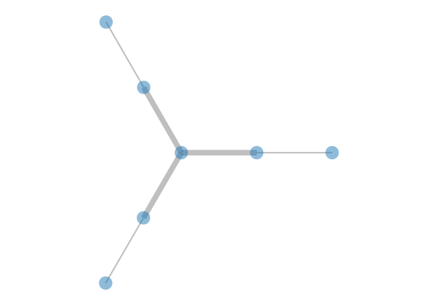
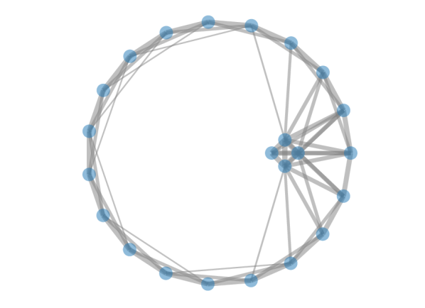
(a) kNN Graph

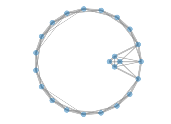
(b) LLE Graph

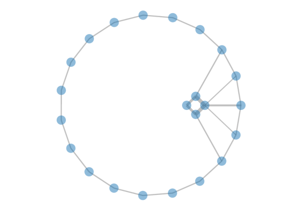
(c) NNK Graph

Figure 6: Graph constructions in synthetic data settings. Unlike kNN and LLE, NNK achieves a sparse representation where the relative locations of nodes in the neighborhood are key. In the seven-node example (top row), the node in the center has only three direct neighbors, which in turn are neighbors of nodes extending the graph further in those three directions. Graphs are constructed with ${\textnormal{k}}=5$ and Gaussian kernel ($\sigma=1$). Edge thickness indicates neighbor weights normalized globally to have values in $[0,1]$.

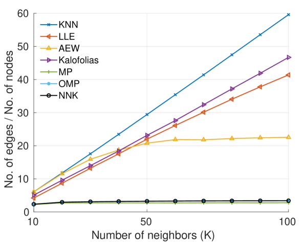
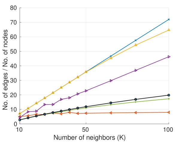
Figure 7: Ratio of the number of edges (with weights $\geq 10^{-8}$) to the number of nodes. Left: Noisy Swiss Roll (N=5000, d=3), Right: MNIST (N=1000, d=784). The sparsity of NNK, MP, OMP graphs saturates for increasing k and is reflective of the intrinsic dimensionality of the data.

5.2.1 Sparsity and runtime complexity

Graph sparsity, measured as the ratio of the number of edges to the number of nodes, is desirable for downstream graph analysis tasks to scale well for large data sets [77]. Unlike a kNN graph, where sparsity is controlled by the choice of k, an NNK graph provides an adaptive sparse representation. Figure 6 presents two examples to compare the NNK graph sparsity with that of the kNN and LLE graphs. In Figure 7, we show the effect of parameter k on the sparsity of various graph methods on a synthetic and real dataset. We see that the MP, OMP, and NNK algorithms lead to the sparsest graph representations. Note that LLE graphs suffer from unstable optimization due to the high dimensionality of the features in the real dataset. Thus, the observed sparsity, in this case, is not reflective of a good graph and is only a shortcoming of the optimization (weights $<10^{-8}$).

As shown in Figure 8, the NNK framework outperforms other methods in terms of both sparsity and the time required to construct the graphs. An OMP graph construction produces an equivalent graph to NNK at a $10\times$ slower runtime. MP method provides a faster alternative to OMP but still remains slow with runtime $2.5\times$ that of NNK.

5.2.2 Label Propagation

We evaluate the quality of the constructed graphs based on their performance in a downstream semi-supervised learning (SSL) task using label propagation [54]. We consider subsets of digits datasets, such as USPS and MNIST, for the experiment. For USPS, we sample each class non-uniformly based on its labels as in [54, 47]. For MNIST, we use $100$ randomly selected samples for each digit class to create one instance of a $1000$ sample dataset ($100$ samples/class $\times$ $10$ digit classes). Fig. 8 shows the average classification error with different graph constructions for an increasing percentage of available labels (randomly selected) and different choices of parameter k. We see that basis pursuit and NNK perform best with both combinatorial (${\bm{L}}$) and symmetric normalized Laplacians (${\mathcal{L}}$) in label propagation for all settings. In particular, we note that NNK and OMP-based constructions result in the same graph structure and performance, as identified in our analysis in Sections 3.4.1 and 4.4, but with a significant difference in runtimes (NNK approach requires much less time compared to OMP).

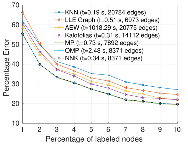
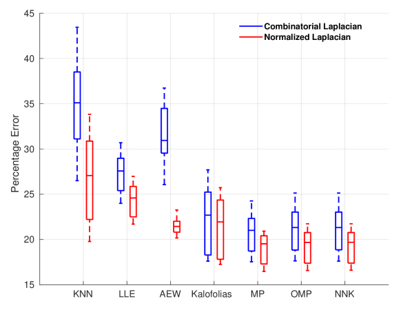
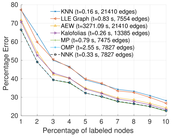
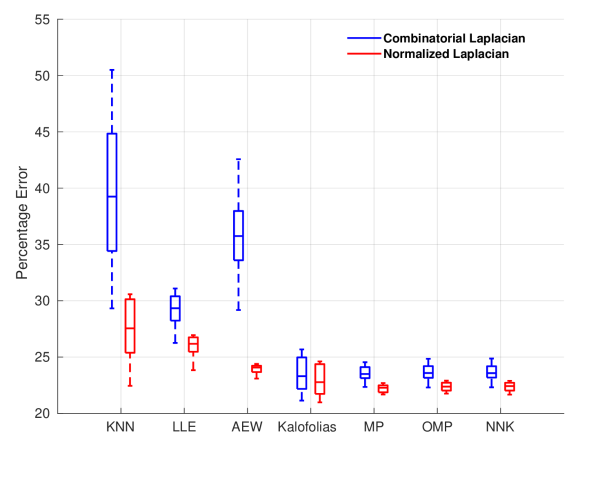
Figure 8: SSL performance (mean over 10 different subsets with 10 random initialization of available labels) with graphs constructed by different algorithms. Left column: Classification error at different percentage of labeled data on USPS (top row) and MNIST (bottom row) dataset with ${\textnormal{k}}=30$. The time taken and the sparsity of the constructed graphs is indicated as part of the legend. Right column: Boxplots showing the robustness of graph constructions using ${\bm{L}}$ and ${\mathcal{L}}$ Laplacians for different choices of k ($10,15,\dots,50$) in SSL task with $10\%$ labeled data on USPS and MNIST.

5.2.3 Laplacian Eigenmaps

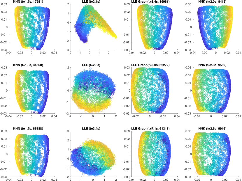
Figure 9: Two-dimensional embedding learned by different algorithms. Left:  Swiss roll, Right: Severed sphere. Each row corresponds to different choice of ${\textnormal{k}}=10,20,40$ (top to bottom). We include the time taken to construct the graph and the number of edges obtained for each method in the subplot title. We see that NNK graphs produce a robust embedding for both datasets with the sparsity of the graph constructed correlating with the intrinsic dimension of the dataset.

We demonstrate the effectiveness of the NNK graph construction in manifold learning using Laplacian Eigenmaps [78] with two standard synthetic datasets, namely, Swiss roll ($N=5000,d=3$) and Severed sphere ($N=3000,d=3$). The embedding obtained using NNK is compared to that of kNN, LLE [24] graphs, and that of the original LLE algorithm [42]. Figure 9 presents a visual comparison of the embedding obtained using different methods and their robustness to the choice of k. We see that NNK graphs have better sparsity, runtime, and robustness in the embeddings obtained relative to the baselines. Moreover, the eigenmaps computation using NNK graphs is significantly faster due to the sparsity of the graph constructed. We note that the sparsity in NNK graphs captures the intrinsic dimensionality of the data, where the ratio of the number of edges to the number of data points corresponds to the dimension of the manifold associated with the datasets, namely, $2$ for Swiss roll corresponding to a plane and $3$ for the Severed sphere indicating that the data is close to a $3$-dimensional surface.

6 Conclusion

We introduced a novel view of neighborhoods where we show that neighborhoods are non-negative sparse signal approximations. We then use this perspective to propose an improved approach, Non-Negative Kernel Regression (NNK), for neighborhood and graph constructions. We also present $l_{1}$-regularized and greedy pursuit approaches to neighborhood definition while establishing its connection to our proposed NNK. We characterize the geometry of proposed neighborhood construction via the kernel ratio interval theorem and establish its implication in non-distance based kernels and other non-negative sparse approximation problems. Our experiments demonstrate that NNK performs better than earlier methods in neighborhood classification and graph-based semi-supervised and manifold learning. Further, we show that our approach leads to the sparsest solutions and is more robust to hyperparameters involved in both neighborhood and graph constructions. NNK has a desirable runtime complexity and can leverage neighborhood search tools developed for kNN. Moreover, the local nature of the NNK algorithm allows for further runtime improvements via parallelization and additional memory. Future work will focus on investigating the relationship between kernel parameters and geometry, addressing the impact of noise in neighborhood definitions, and developing multi-scale neighborhood representations.

Sarath Shekkizhar received his bachelor (Electronics and Communication) and double master (Electrical Engineering, Computer Science) degrees from National Institute of Technology, Tiruchirappalli, India and University of Southern California (USC), Los Angeles, USA, respectively. He is currently working on his doctoral degree in Electrical and Computer Engineering at USC and is the recipient of the IEEE best student paper award at ICIP 2020. His research interests include graph signal processing, non-parametric methods, and machine learning.

Antonio Ortega received his undergraduate and doctoral degrees from the Universidad Politécnica de Madrid, Madrid, Spain and Columbia University, New York, USA, respectively. In 1994 he joined the Electrical Engineering department at the University of Southern California, where he is currently Dean’s Professor. He was the Editor-in-Chief of the IEEE Transactions of Signal and Information Processing over Networks and recently served as a member of the Board of Governors of the IEEE Signal Processing Society. His recent research work is focused on graph signal processing, machine learning, multimedia compression and wireless sensor networks. Over $40$ PhD students have completed their PhD under his supervision and his work has led to over $400$ publications in international conferences and journals, as well as several patents. He is the author of the book Introduction to Graph Signal Processing published by Cambridge University Press in 2022.

Appendix A General Kernel Ratio Interval

Theorem 3.

Given a three node scenario as in Fig.2 and a Mercer kernel, the necessary and sufficient condition for two data points $i$ and $j$ to be connected to $q$ in an NNK framework is

$$\frac{{\bm{K}}_{i,j}}{{\bm{K}}_{j,j}}<\frac{{\bm{K}}_{q,i}}{{\bm{K}}_{q,j}}<\frac{{\bm{K}}_{i,i}}{{\bm{K}}_{i,j}}$$ (25)

Remark 1.

Note that the general KRI condition in Theorem 3 is independent of the self-similarity or norm of the data to be represented, i.e., ${\bm{K}}_{q,q}$. This makes intuitive sense from a neighborhood definition or signal approximation point of view: the self-similarity of $q$ does not change the projection order of neighbors (nearest to farthest) since ${\bm{K}}_{q,q}$ is non-negative for Mercer kernels.

$$\frac{{\bm{K}}_{q,i}}{{\bm{K}}_{i,i}}\leq\frac{{\bm{K}}_{q,j}}{{\bm{K}}_{j,j}}\iff\frac{{\bm{K}}_{q,i}}{{\bm{K}}_{q,q}{\bm{K}}_{i,i}}\leq\frac{{\bm{K}}_{q,j}}{{\bm{K}}_{q,q}{\bm{K}}_{j,j}}$$

Remark 2.

It should be also noted that if the data to be selected as neighbors (e.g., $i,j$) have unit self-similarity, then the condition of Theorem 3 reduces to the simpler KRI condition of Theorem 1 irrespective of the self-similarity of the query point being approximated i.e., ${\bm{K}}_{q,q}$.

Appendix B Proofs

B.1 Karush-Kuhn-Tucker optimality conditions of NNK

A solution to (6) satisfies the Karush-Kuhn-Tucker (KKT) conditions as listed below.

$${\bm{K}}_{S,S}{\bm{\theta}}-{\bm{K}}_{S,q}-{\bm{\lambda}}={\bm{0}}$$ (26a)

$${\bm{\lambda}}^{\top}{\bm{\theta}}=0$$ (26b)

$${\bm{\theta}}\geq{\bm{0}},\quad{\bm{\lambda}}\geq{\bm{0}}$$ (26c)

We will use these conditions to analyze and prove the properties of the NNK framework in the following sections.

B.2 Proof of Proposition 1

Proof.

An optimum solution at node $q$ satisfies the KKT conditions, specifically the stationarity condition (26a)

$${\bm{K}}_{S,S}{\bm{\theta}}={\bm{K}}_{S,q}\quad s.t\quad{\bm{\theta}}_{S}\geq\mathbf{0}$$ (27)

This can be interpreted as a solution to a set of linear equations under constraint.

$$\sum_{j\in S}\theta_{j}\;\kappa({\bm{x}}_{i},{\bm{x}}_{j})=\kappa({\bm{x}}_{q},{\bm{x}}_{i})\quad\forall i\in S,\;{\bm{\theta}}\geq\bf 0$$ (28)

Local Linear Embedding (LLE) with positive weight constraint minimizes

$${\bm{Z}}^{\top}{\bm{Z}}{\bm{w}}=1,\text{ where }{\bm{Z}}={\bm{X}}_{S}-{\bm{x}}_{q}\quad s.t\;\sum_{i\in S}w_{i}=1,\;{\bm{w}}\geq\bf 0$$

Let ${\bm{M}}={\bm{Z}}^{\top}{\bm{Z}}$, i.e.,

$${\bm{M}}_{i,j}=({\bm{x}}_{i}-{\bm{x}}_{q})^{\top}({\bm{x}}_{j}-{\bm{x}}_{q}),\quad\forall\;i,j\in S.$$

Then, LLE objective corresponds to solving a set of equations with constraints, namely

$$\sum_{j\in S}w_{j}\;({\bm{x}}_{i}-{\bm{x}}_{q})^{\top}({\bm{x}}_{j}-{\bm{x}}_{q})=1\quad\forall i\in S$$

$$\text{such that }\;\sum_{i\in S}w_{i}=1,\quad{\bm{w}}\geq\bf 0$$ (29)

An equivalent set of equations is given by,

$$\sum_{j\in S}\mu_{j}\|{\bm{x}}_{j}-{\bm{x}}_{q}\|\|{\bm{x}}_{i}-{\bm{x}}_{q}\|\,\frac{({\bm{x}}_{j}-{\bm{x}}_{q})^{\top}({\bm{x}}_{i}-{\bm{x}}_{q})}{2\|{\bm{x}}_{j}-{\bm{x}}_{q}\|\|{\bm{x}}_{i}-{\bm{x}}_{q}\|}=\frac{1}{2}.$$

Since each weight $w_{j}$ is positive it can be factored as a product of positive terms, specifically let

$$w_{j}=\mu_{j}\,\|{\bm{x}}_{j}-{\bm{x}}_{q}\|\;\|{\bm{x}}_{i}-{\bm{x}}_{q}\|$$

Further, using the constraint that weights add up to one, equation (29) is rewritten as

$$\sum_{j\in S}w_{j}\,\frac{({\bm{x}}_{j}-{\bm{x}}_{q})^{\top}({\bm{x}}_{i}-{\bm{x}}_{q})}{2\|{\bm{x}}_{j}-{\bm{x}}_{q}\|\|{\bm{x}}_{i}-{\bm{x}}_{q}\|} =1-\sum_{j\in S}\frac{w_{j}}{2}$$

$$\sum_{j\in S}w_{j}\left(\frac{1}{2}+\frac{({\bm{x}}_{j}-{\bm{x}}_{q})^{\top}({\bm{x}}_{i}-{\bm{x}}_{q})}{2\|{\bm{x}}_{j}-{\bm{x}}_{q}\|\|{\bm{x}}_{i}-{\bm{x}}_{q}\|}\right) =1$$

$$\forall i\in S, \;{\bm{w}}\geq\bf 0$$ (30)

Combined with lemma 3.1, we see that equation (30) is exactly the NNK objective with the kernel at node $q$ defined as in equation (7), i.e.,

$$\sum_{j\in S}w_{j}\;\kappa_{q}({\bm{x}}_{i},{\bm{x}}_{j})=\kappa_{q}({\bm{x}}_{q},{\bm{x}}_{i})\quad\forall i\in S,\;{\bm{w}}\geq\bf 0$$ (31)

∎

Lemma 3.1.

$\underset{{\bm{h}}\to 0}{\lim}\;\kappa_{q}({\bm{x}}_{q}+{\bm{h}},{\bm{x}}_{i})=1$

Proof.

$$\kappa_{q}({\bm{x}}_{q},{\bm{x}}_{i})=\frac{1}{2}+\frac{({\bm{x}}_{q}-{\bm{x}}_{q})^{\top}({\bm{x}}_{i}-{\bm{x}}_{q})}{2\|{\bm{x}}_{q}-{\bm{x}}_{q}\|\|{\bm{x}}_{i}-{\bm{x}}_{q}\|}$$

The above expression is indeterminate in its current form. Let’s consider the limit of the expression.

$$\underset{{\bm{h}}\to 0}{\lim}\;\kappa_{q}({\bm{x}}_{q}+{\bm{h}},{\bm{x}}_{i}) =\underset{{\bm{h}}\to 0}{\lim}\;\frac{1}{2}+\frac{({\bm{x}}_{q}+{\bm{h}}-{\bm{x}}_{q})^{\top}({\bm{x}}_{i}-{\bm{x}}_{q})}{2\|{\bm{x}}_{q}+{\bm{h}}-{\bm{x}}_{q}\|\|{\bm{x}}_{i}-{\bm{x}}_{q}\|}$$

$$=\frac{1}{2}+\underset{{\bm{h}}\to 0,\,\alpha\to 0}{\lim}\;\frac{\|{\bm{x}}_{i}-{\bm{x}}_{q}\|\|{\bm{h}}\|\cos\alpha}{2\|{\bm{x}}_{i}-{\bm{x}}_{q}\|\|{\bm{h}}\|}$$

where $\alpha$ is the angle between $({\bm{x}}_{i}-{\bm{x}}_{q})$ and ${\bm{h}}$.

$$\implies\underset{{\bm{h}}\to 0}{\lim}\;\kappa_{q}({\bm{x}}_{q}+{\bm{h}},{\bm{x}}_{i}) =1\quad\text{since}\quad\underset{\alpha\to 0}{\lim}\cos\alpha=1$$

∎

B.3 Proof of Proposition 2

Proof.

The Karush-Kuhn-Tucker (KKT) optimality conditions for equation (9) are

$${\bm{K}}_{{\mathcal{D}},{\mathcal{D}}}{\bm{\theta}}^{*}-{\bm{K}}_{{\mathcal{D}},q}+\eta{\bm{1}}-{\bm{\lambda}}={\bm{0}}$$ (32a)

$$\lambda_{j}\theta^{*}_{j}=0$$ (32b)

$${\bm{\theta}}^{*}\geq{\bm{0}},\quad{\bm{\lambda}}\geq{\bm{0}}$$ (32c)

The non negativity of both ${\bm{K}}_{{\mathcal{D}},{\mathcal{D}}}$ (kernels are non-negative by design) and ${\bm{\theta}}^{*}$ (by constraint) ensures ${\bm{K}}_{{\mathcal{D}},{\mathcal{D}}}{\bm{\theta}}^{*}\geq 0$. This implies that the stationarity condition (32a) is satisfied only when $\eta\mathbf{1}-{\bm{K}}_{{\mathcal{D}},{\mathcal{D}}}-{\bm{\lambda}}\leq\mathbf{0}$. Combining with the slackness condition (32b) we have the results of the proposition.

$$\eta-{\bm{K}}_{q,j}>0\implies \lambda_{j}>0\quad\because\eta-{\bm{K}}_{q,j}-\lambda_{j}\leq 0$$

$$\implies \theta^{*}_{j}=0\quad\because\lambda_{j}\theta^{*}_{j}=0\qed$$

B.4 Proof of Proposition 3

Proof.

Under the partition, the objective of NNK (6) can be rewritten using block partitioned matrices

$${\bm{K}}_{S,S}=\begin{bmatrix}{\bm{K}}_{P,P}&{\bm{K}}_{P,\bar{P}}\\ {\bm{K}}^{\top}_{P,\bar{P}}&{\bm{K}}_{\bar{P},\bar{P}}\end{bmatrix},\quad{\bm{K}}_{S,q}=\begin{bmatrix}{\bm{K}}_{P,q}\\ {\bm{K}}_{\bar{P},q}\end{bmatrix}.$$

The optimization for the sub problem corresponding to indices in ${\bm{\theta}}_{P}$ is

$$\underset{{\bm{\theta}}_{P}:{\bm{\theta}}_{P}\geq 0}{\min}\;\;\frac{1}{2}{\bm{\theta}}^{\top}_{P}{\bm{K}}_{P,P}{\bm{\theta}}_{P}-{\bm{K}}^{\top}_{P,q}{\bm{\theta}}_{P}.$$ (33)

An optimal solution to this sub objective (${\bm{\theta}}^{*}_{P}$) satisfies the KKT conditions (26) namely,

$${\bm{K}}_{P,P}{\bm{\theta}}^{*}_{P}-{\bm{K}}_{P,q}-{\bm{\lambda}}_{P}=\bf 0$$

$${\bm{\lambda}}_{P}^{\top}{\bm{\theta}}^{*}_{P}=0$$

$${\bm{\theta}}^{*}_{P}\geq\bf 0,\;{\bm{\lambda}}_{P}\geq\bf 0$$

Specifically, given ${\bm{\theta}}^{*}_{P}>\bf 0$, the solution satisfies the stationarity condition (eq. 26a),

$${\bm{K}}_{P,P}{\bm{\theta}}^{*}_{P}-{\bm{K}}_{P,q}={\bm{0}}\qquad\because{\bm{\lambda}}_{P}={\bm{0}}$$ (34)

The zero augmented solution with ${\bm{\theta}}_{\bar{P}}=\bf 0$ is optimal for the original problem provided

$$\begin{bmatrix}{\bm{K}}_{P,P}&{\bm{K}}_{P,\bar{P}}\\ {\bm{K}}^{\top}_{P,\bar{P}}&{\bm{K}}_{\bar{P},\bar{P}}\end{bmatrix}\begin{bmatrix}{\bm{\theta}}^{*}_{P}\\ \bf 0\end{bmatrix}-\begin{bmatrix}{\bm{K}}_{P,q}\\ {\bm{K}}_{\bar{P},q}\end{bmatrix}-\begin{bmatrix}{\bm{\lambda}}_{P}\\ {\bm{\lambda}}_{\bar{P}}\end{bmatrix}=\bf 0$$

$$\begin{bmatrix}{\bm{\lambda}}_{P}&{\bm{\lambda}}_{\bar{P}}\end{bmatrix}\begin{bmatrix}{\bm{\theta}}^{*}_{P}\\ \bf 0\end{bmatrix}=0$$

$$\begin{bmatrix}{\bm{\theta}}^{*}_{P}\\ \bf 0\end{bmatrix}\geq\bf 0,\;\begin{bmatrix}{\bm{\lambda}}_{P}\\ {\bm{\lambda}}_{\bar{P}}\end{bmatrix}\geq\bf 0$$

Given the optimality conditions on ${\bm{\theta}}^{*}_{P}$ , the conditions for $[{\bm{\theta}}^{*}_{P}\;{\bm{\theta}}_{\bar{P}}]^{\top}$ to be optimal requires

$${\bm{K}}^{\top}_{P,\bar{P}}{\bm{\theta}}^{*}_{P}-{\bm{K}}_{\bar{P},q}-{\bm{\lambda}}_{\bar{P}}=\bf 0\quad{\bm{\lambda}}_{\bar{P}}\geq\bf 0$$

$$\implies{\bm{K}}^{\top}_{P,\bar{P}}{\bm{\theta}}^{*}_{P}-{\bm{K}}_{\bar{P},q}\geq\bf 0$$ (35)

∎

B.5 Proof of Theorem 1

B.5.1 Main proof

Proof.

An exact solution to objective (6) without the constraint on ${\bm{\theta}}$ at a data point $q$ and set $S=\{i,j\}$ satisfies

$$\begin{bmatrix}1&{\bm{K}}_{i,j}\\ {\bm{K}}_{i,j}&1\end{bmatrix}\begin{bmatrix}\theta_{i}\\ \theta_{j}\end{bmatrix}=\begin{bmatrix}{\bm{K}}_{q,i}\\ {\bm{K}}_{q,j}\end{bmatrix}$$ (36)

$$\iff\theta_{i}+\theta_{j}{\bm{K}}_{i,j}={\bm{K}}_{q,i}$$

$$\theta_{i}{\bm{K}}_{i,j}+\theta_{j}={\bm{K}}_{q,j}$$

Taking the ratio of the equations

$$\frac{\theta_{i}+\theta_{j}{\bm{K}}_{i,j}}{\theta_{i}{\bm{K}}_{i,j}+\theta_{j}}=\frac{{\bm{K}}_{q,i}}{{\bm{K}}_{q,j}}$$ (37)

Now, $0\leq{\bm{K}}_{i,j}\leq 1$, where ${\bm{K}}_{i,j}=1$ if and only if the points are same. Without loss of generality, let us assume points $i$ and $j$ are distinct. Then,

$${\bm{K}}_{i,j}<1\leq\frac{{\bm{K}}_{q,i}}{{\bm{K}}_{q,j}} \iff{\bm{K}}_{i,j}<\frac{\theta_{i}+\theta_{j}{\bm{K}}_{i,j}}{\theta_{i}{\bm{K}}_{i,j}+\theta_{j}}$$

$$\iff\theta_{i}+\theta_{j}{\bm{K}}_{i,j} >\theta_{i}{\bm{K}}^{2}_{i,j}+\theta_{j}{\bm{K}}_{i,j}$$

$$\iff\theta_{i}>\theta_{i}{\bm{K}}^{2}_{i,j} \iff\theta_{i}>0$$

$$\therefore\quad\theta_{i}>0 \iff{\bm{K}}_{i,j}<\frac{{\bm{K}}_{q,i}}{{\bm{K}}_{q,j}}$$ (38)

Similarly,

$$\frac{{\bm{K}}_{q,i}}{{\bm{K}}_{q,j}}<\frac{1}{{\bm{K}}_{i,j}} \iff\frac{\theta_{i}+\theta_{j}{\bm{K}}_{i,j}}{\theta_{i}{\bm{K}}_{i,j}+\theta_{j}}<\frac{1}{{\bm{K}}_{i,j}}$$

$$\iff\theta_{i}{\bm{K}}_{i,j}+\theta_{j} >\theta_{i}{\bm{K}}_{i,j}+\theta_{j}{\bm{K}}^{2}_{i,j}$$

$$\iff\theta_{j}>\theta_{j}{\bm{K}}^{2}_{i,j} \iff\theta_{j}>0$$

$$\therefore\quad\theta_{j}>0 \iff\frac{{\bm{K}}_{q,i}}{{\bm{K}}_{q,j}}<\frac{1}{{\bm{K}}_{i,j}}$$ (39)

Equations (38) and (39) give the necessary and sufficient condition of (13).

$${\bm{K}}_{i,j}<\frac{{\bm{K}}_{q,i}}{{\bm{K}}_{q,j}}<\frac{1}{{\bm{K}}_{i,j}}.$$

∎

B.5.2 Proof of Corollary 1.1

Proof.

Let $j$ be a node beyond the plane as in Figure 3(a). For a Gaussian kernel with bandwidth $\sigma$, ${\bm{K}}_{q,i}>{\bm{K}}_{q,j}$. Thus, condition corresponding to (38) is satisfied,

$$\frac{{\bm{K}}_{q,i}}{{\bm{K}}_{q,j}}>1>{\bm{K}}_{i,j}\implies\theta_{i}>0$$

Let $\|{\bm{x}}_{q}-{\bm{x}}_{i}\|=a,\;\|{\bm{x}}_{q}-{\bm{x}}_{j}\|=b\;$ and $\alpha$ be the angle between the difference vectors. Then,

$$\frac{{\bm{K}}_{q,i}}{{\bm{K}}_{q,j}} =\exp\left(\frac{1}{2\sigma^{2}}(b^{2}-a^{2})\right)$$

$${\bm{K}}_{i,j} =\exp\left(-\frac{1}{2\sigma^{2}}((b\cos\alpha-a)^{2}+(b\sin\alpha)^{2})\right)$$

$${\bm{K}}_{i,j} =\exp\left(-\frac{1}{2\sigma^{2}}(b^{2}+a^{2}-2ab\cos\alpha)\right)$$

$$\frac{1}{{\bm{K}}_{i,j}} =\exp\left(-\frac{1}{2\sigma^{2}}(b^{2}+a^{2}-2ab\cos\alpha)\right)$$

Now, the condition on $\theta_{j}$, the inequality (39) is reduced as

$$\frac{{\bm{K}}_{q,i}}{{\bm{K}}_{q,j}} <\frac{1}{{\bm{K}}_{i,j}}$$

$$\exp\left(\frac{1}{2\sigma^{2}}(b^{2}-a^{2})\right) <\exp\left(\frac{1}{2\sigma^{2}}(b^{2}+a^{2}-2ab\cos\alpha)\right)$$

$$\exp\left(-\frac{a^{2}}{2\sigma^{2}}\right) <\exp\left(\frac{1}{2\sigma^{2}}(a^{2}-2ab\cos\alpha)\right)$$

$$\exp\left(\frac{1}{2\sigma^{2}}ab\cos\alpha\right) <\exp\left(\frac{a^{2}}{2\sigma^{2}}\right)$$

$$b\cos\alpha<a \iff\theta_{j}=0\quad\forall\;b\cos\alpha>a$$

The condition $b\cos\alpha>a$ corresponds to a hyperplane corresponding to points that belong to the half space not containing $q$. ∎

B.5.3 Proof of Corollary 1.2

Proof.

Statements A and B are related in that one is the contrapositive of the other. Here we prove statement A.
Equation (11) can be interpreted as the boundaries of a convex polytope (${\mathcal{P}}$) formed by the half planes,

$$boundary({\mathcal{P}})=\{{\bm{K}}^{\top}_{P,i}{\bm{\theta}}_{P}={\bm{K}}_{q,i}\quad i\in P\}$$ (40)

The interior of the polytope formed by the half planes is

$$interior({\mathcal{P}})=\{p\;:\;{\bm{K}}^{\top}_{P,p}{\bm{\theta}}_{P}-{\bm{K}}_{q,p}<0\}.$$ (41)

Thus,

$${\bm{K}}^{\top}_{P,j}{\bm{\theta}}_{P}-{\bm{K}}_{q,i}\geq 0$$ (42)

corresponds to a point outside ${\mathcal{P}}$. Now, to prove

$$\exists i\in P\;\colon\;\frac{{\bm{K}}_{q,i}}{{\bm{K}}_{q,j}}\geq\frac{1}{{\bm{K}}_{i,j}}$$

Let’s assume there exists no such $i$. Then

$$\forall i\in P\;\colon\;\frac{{\bm{K}}_{q,i}}{{\bm{K}}_{q,j}} <\frac{1}{{\bm{K}}_{i,j}}$$

$${\bm{K}}_{q,i}{\bm{K}}_{i,j} <{\bm{K}}_{q,j}$$

$$\left({\bm{K}}^{\top}_{P,i}{\bm{\theta}}_{P}\right){\bm{K}}_{i,j} <{\bm{K}}_{q,j}\quad\quad\because i\in{\mathcal{P}}$$

$$\left({\bm{K}}_{P,i}{\bm{K}}_{i,j}\right)^{\top}{\bm{\theta}}_{P} <{\bm{K}}_{q,j}$$ (43)

Using the triangle inequality corresponding to kernels for each term in $P$, we have

$${\bm{K}}^{\top}_{P,j}{\bm{\theta}}_{P} <{\bm{K}}_{q,j}\qquad\text{since }{\bm{K}}_{P,q}\leq{\bm{K}}_{P,i}{\bm{K}}_{i,j}$$ (44)

Equation (44) contradicts our earlier statement (eq. 42) on point $j$, namely, $j$ lies outside ${\mathcal{P}}$ and hence does not belong to the interior as defined in equation (41). Thus,

$$\exists\;i\;\in\;P\;\colon\;\frac{{\bm{K}}_{q,i}}{{\bm{K}}_{q,j}}\geq\frac{1}{{\bm{K}}_{i,j}}$$

∎

B.6 Proof of Proposition 4

Proof.

$$\tilde{d}^{2}(i,j) =({\bm{\phi}}_{i}-{\bm{\phi}}_{j})^{t}({\bm{\phi}}_{i}-{\bm{\phi}}_{j})$$

$$={\bm{\phi}}_{i}^{t}{\bm{\phi}}_{i}-{\bm{\phi}}_{i}^{t}{\bm{\phi}}_{j}-{\bm{\phi}}_{j}^{t}{\bm{\phi}}_{i}+{\bm{\phi}}_{j}^{t}{\bm{\phi}}_{j}$$

$$=2-2{\bm{\phi}}_{i}^{t}{\bm{\phi}}_{j}\;\because\|{\bm{\phi}}_{i}\|=\|{\bm{\phi}}_{j}\|=1$$

$$=2-2\leavevmode\nobreak\ \kappa({\bm{x}}_{i},{\bm{x}}_{j})$$

∎

B.7 Proof of Theorem 2

Proof.

The proof follows from the kernel ratio interval Theorem 1 and proposition 4.

Consider the condition for $\theta_{j}\;\neq\;0$:

$$\frac{{\bm{K}}_{q,i}}{{\bm{K}}_{q,j}}<\frac{1}{{\bm{K}}_{i,j}}\iff{\bm{K}}_{q,i}{\bm{K}}_{i,j} <{\bm{K}}_{q,j}$$

$$\left[1-\frac{\tilde{d}^{2}(q,i)}{2}\right]\left[1-\frac{\tilde{d}^{2}(i,j)}{2}\right] <\left[1-\frac{\tilde{d}^{2}(q,j)}{2}\right]$$

$$1-\frac{\tilde{d}^{2}(q,i)}{2}-\frac{\tilde{d}^{2}(i,j)}{2}+\frac{\tilde{d}^{2}(q,i)\tilde{d}^{2}(i,j)}{4} <1-\frac{\tilde{d}^{2}(q,j)}{2}$$

$$\tilde{d}^{2}(q,i)+\tilde{d}^{2}(i,j)-\tilde{d}^{2}(q,j) >\frac{\tilde{d}^{2}(q,i)\tilde{d}^{2}(i,j)}{2}$$

The proof for $\theta_{i}$ can be derived using a similar argument. ∎

B.8 Proof of Theorem 3

Proof.

A solution to the NNK objective without the constraint on ${\bm{\theta}}$ at data point $q$ and set $S=\{i,j\}$ satisfies

$$\begin{bmatrix}{\bm{K}}_{i,i}&{\bm{K}}_{i,j}\\ {\bm{K}}_{i,j}&{\bm{K}}_{j,j}\end{bmatrix}\begin{bmatrix}\theta_{i}\\ \theta_{j}\end{bmatrix}=\begin{bmatrix}{\bm{K}}_{q,i}\\ {\bm{K}}_{q,j}\end{bmatrix}$$ (45)

$$\iff\theta_{i}{\bm{K}}_{i,i}+\theta_{j}{\bm{K}}_{i,j}={\bm{K}}_{q,i}$$

$$\theta_{i}{\bm{K}}_{i,j}+\theta_{j}{\bm{K}}_{j,j}={\bm{K}}_{q,j}$$

Taking the ratio of the above equations

$$\frac{\theta_{i}{\bm{K}}_{i,i}+\theta_{j}{\bm{K}}_{i,j}}{\theta_{i}{\bm{K}}_{i,j}+\theta_{j}{\bm{K}}_{j,j}}=\frac{{\bm{K}}_{q,i}}{{\bm{K}}_{q,j}}$$ (46)

In the following statements, we will show that under conditions of equation (25) that the solutions will be positive and vice versa. Now, ${\bm{K}}^{2}_{i,j}\leq{\bm{K}}_{i,i}{\bm{K}}_{j,j}$. This is because kernels with RKHS property are positive definite functions, with equality iff the points $i$ and $j$ are the same. Without loss of generality, let us assume points $i$ and $j$ are distinct. Then,

$$\frac{{\bm{K}}_{i,j}}{{\bm{K}}_{j,j}}<\frac{{\bm{K}}_{q,i}}{{\bm{K}}_{q,j}}\iff \frac{{\bm{K}}_{i,j}}{{\bm{K}}_{j,j}}<\frac{\theta_{i}{\bm{K}}_{i,i}+\theta_{j}{\bm{K}}_{i,j}}{\theta_{i}{\bm{K}}_{i,j}+\theta_{j}{\bm{K}}_{j,j}}$$

$$\iff\theta_{i}{\bm{K}}_{i,i}{\bm{K}}_{j,j}+\theta_{j}{\bm{K}}_{i,j}{\bm{K}}_{j,j} >\theta_{i}{\bm{K}}^{2}_{i,j}+\theta_{j}{\bm{K}}_{j,j}{\bm{K}}_{i,j}$$

$$\iff\theta_{i}{\bm{K}}_{i,i}{\bm{K}}_{j,j} >\theta_{i}{\bm{K}}^{2}_{i,j}$$

$$\iff\theta_{i}>0\qquad \because{\bm{K}}^{2}_{i,j}<{\bm{K}}_{i,i}{\bm{K}}_{j,j}$$

Thus,

$$\therefore\theta_{i}>0\iff\frac{{\bm{K}}_{i,j}}{{\bm{K}}_{j,j}}<\frac{{\bm{K}}_{q,i}}{{\bm{K}}_{q,j}}$$ (47)

Similar result holds for $\theta_{j}$, namely,

$$\theta_{j}>0\iff\frac{{\bm{K}}_{q,i}}{{\bm{K}}_{q,j}}<\frac{{\bm{K}}_{i,i}}{{\bm{K}}_{i,j}}.$$ (48)

Equations (47) and (48) combined give the necessary and sufficient condition in the theorem and completes the proof.

$$\frac{{\bm{K}}_{i,j}}{{\bm{K}}_{j,j}}<\frac{{\bm{K}}_{q,i}}{{\bm{K}}_{q,j}}<\frac{{\bm{K}}_{i,i}}{{\bm{K}}_{i,j}}$$

∎

References

- [1] M. Pelillo, “Alhazen and the nearest neighbor rule,” Pattern Recognition Letters, vol. 38, pp. 34–37, 2014.
- [2] E. Fix and J. L Hodges, “Discriminatory analysis-nonparametric discrimination: Small sample performance,” Tech. Rep., California Univ. Berkeley, 1952.
- [3] T. Cover and P. Hart, “Nearest neighbor pattern classification,” IEEE Trans. on Info. Theory, 1967.
- [4] E. A Nadaraya, “On estimating regression,” Theory of Probability & Its Applications, 1964.
- [5] G. S Watson, “Smooth regression analysis,” Sankhyā: The Indian J. of Statistics, Series A, 1964.
- [6] G. Biau and L. Devroye, Lectures on the Nearest Neighbor method, Springer, 2015.
- [7] A. Ortega, P. Frossard, J. Kovačević, J. Moura, and P. Vandergheynst, “Graph signal processing: Overview, challenges, and applications,” Proceedings of the IEEE, 2018.
- [8] A. Ortega, Introduction to graph signal processing, Cambridge University Press, 2022.
- [9] W. L. Hamilton, R. Ying, and J. Leskovec, “Representation Learning on Graphs: Methods and Applications,” 2017.
- [10] I. Chami, S. Abu-El-Haija, B. Perozzi, C. Ré, and K. Murphy, “Machine learning on graphs: A model and comprehensive taxonomy,” Journal of Machine Learning Research, vol. 23, no. 89, pp. 1–64, 2022.
- [11] M. Maiker, U. von Luxburg, and M. Hein, “Influence of graph construction on graph-based clustering measures,” Advances in Neural Info. Processing Systems, 2009.
- [12] C. A. R. De Sousa, S. O. Rezende, and G. Batista, “Influence of graph construction on semi-supervised learning,” in Joint European Conf. on Machine Learning and Knowledge Discovery in Databases. Springer, 2013, pp. 160–175.
- [13] C. J Stone, “Consistent nonparametric regression,” The Annals of Statistics, 1977.
- [14] L. Devroye, L. Györfi, and G. Lugosi, A probabilistic theory of pattern recognition, Springer, 2013.
- [15] D. Wettschereck and T. G Dietterich, “Locally adaptive nearest neighbor algorithms,” Advances in Neural Info. Processing Systems, pp. 184–184, 1994.
- [16] L. Baoli, L. Qin, and Y. Shiwen, “An adaptive k-nearest neighbor text categorization strategy,” ACM Trans. on Asian Language Info. Processing (TALIP), vol. 3, no. 4, pp. 215–226, 2004.
- [17] A. Balsubramani, S. Dasgupta, Y. Freund, and S. Moran, “An adaptive nearest neighbor rule for classification,” Advances in Neural Info. Processing Systems, vol. 32, 2019.
- [18] A. K Ghosh, “On nearest neighbor classification using adaptive choice of k,” Journal of computational and graphical statistics, vol. 16, no. 2, pp. 482–502, 2007.
- [19] S. Mullick, S. Datta, and S. Das, “Adaptive learning-based -nearest neighbor classifiers with resilience to class imbalance,” IEEE Trans. on Neural Networks and Learning Systems, 2018.
- [20] O. Anava and K. Levy, “-nearest neighbors: From global to local,” in Advances in Neural Inf. Processing Systems, 2016.
- [21] G. Chen and D. Shah, Explaining the success of nearest neighbor methods in prediction, Now Publishers, 2018.
- [22] D. L Donoho, “Compressed sensing,” IEEE Trans. on Info. Theory, vol. 52, no. 4, pp. 1289–1306, 2006.
- [23] S. Shekkizhar and A. Ortega, “Graph construction from data by Non-Negative Kernel Regression,” in Intl. Conf. on Acoustics, Speech and Signal Processing (ICASSP). IEEE, 2020.
- [24] F. Wang and C. Zhang, “Label propagation through linear neighborhoods,” IEEE Trans. on Knowledge and Data Engineering, 2008.
- [25] M. Karasuyama and H. Mamitsuka, “Adaptive edge weighting for graph-based learning algorithms,” Machine Learning, 2017.
- [26] V. Kalofolias and N. Perraudin, “Large scale graph learning from smooth signals,” in Intl. Conf. on Learning Representations, 2019.
- [27] S. Shekkizhar and A. Ortega, “Efficient graph construction for image representation,” in Intl. Conf. on Image Processing (ICIP). IEEE, 2020, pp. 1956–1960.
- [28] S. Shekkizhar and A. Ortega, “NNK-Means: Data summarization using dictionary learning with non-negative kernel regression,” in 30th European Signal Processing Conf. (EUSIPCO). IEEE, 2022.
- [29] S. Shekkizhar and A. Ortega, “Revisiting local neighborhood methods in machine learning,” in Data Science and Learning Workshop (DSLW). IEEE, 2021.
- [30] S. Shekkizhar and A. Ortega, “Model selection and explainability in neural networks using a polytope interpolation framework,” in 55th Asilomar Conf. on Signals, Systems, and Computers. IEEE, 2021.
- [31] D. Bonet, A. Ortega, J. Ruiz-Hidalgo, and S. Shekkizhar, “Channel redundancy and overlap in convolutional neural networks with channel-wise nnk graphs,” in IEEE Intl. Conf. on Acoustics, Speech and Signal Processing (ICASSP). IEEE, 2022, pp. 4328–4332.
- [32] D. Bonet, A. Ortega, J. Ruiz-Hidalgo, and S. Shekkizhar, “Channel-wise early stopping without a validation set via nnk polytope interpolation,” in Asia-Pacific Signal and Info. Processing Association Annual Summit and Conf. (APSIPA ASC). IEEE, 2021.
- [33] R. Cosentino, S. Shekkizhar, M. Soltanolkotabi, S. Avestimehr, and A. Ortega, “The geometry of self-supervised learning models and its impact on transfer learning,” arXiv:2209.08622, 2022.
- [34] L. Qiao, L. Zhang, S. Chen, and D. Shen, “Data-driven graph construction and graph learning: A review,” Neurocomputing, 2018.
- [35] T. Hofmann, B. Schölkopf, and A. J Smola, “Kernel methods in machine learning,” The annals of statistics, 2008.
- [36] M. A Álvarez, L. Rosasco, and N. D Lawrence, “Kernels for vector-valued functions: A review,” Foundations and Trends® in Mach. Learn., 2012.
- [37] J. Mercer, “Functions of positive and negative type, and their connection with the theory of integral equations,” Philosophical Trans. of the Royal society of London. Series A, 1909.
- [38] N. Aronszajn, “Theory of reproducing kernels,” Trans. of the American mathematical society, 1950.
- [39] B. Kulis, “Metric learning: A survey,” Foundations and trends in machine learning, vol. 5, no. 4, pp. 287–364, 2012.
- [40] F. Wang and J. Sun, “Survey on distance metric learning and dimensionality reduction in data mining,” Data mining and knowledge discovery, vol. 29, no. 2, pp. 534–564, 2015.
- [41] A. Kapoor, H. Ahn, Y.v Qi, and R.W. Picard, “Hyperparameter and kernel learning for graph based semi-supervised classification,” in Advances in Neural Info. Processing Systems, 2005.
- [42] S. T. Roweis and L. K. Saul, “Nonlinear dimensionality reduction by locally linear embedding,” Science, 2000.
- [43] T. Jebara, J. Wang, and S. Chang, “Graph Construction and b-Matching for Semi-Supervised Learning,” Intl. Conf. on Machine Learning, 2009.
- [44] S. Daitch, J. Kelner, and D. Spielman, “Fitting a Graph to Vector Data,” Intl. Conf. on Machine Learning, 2009.
- [45] B. Cheng, J. Yang, S. Yan, Y. Fu, and T. S. Huang, “Learning with l1-graph for image analysis,” IEEE Trans. on Image Processing, 2010.
- [46] S. Han and H. Qin, “Structure aware l1 graph for data clustering,” in AAAI, 2016.
- [47] V. Kalofolias, “How to learn a graph from smooth signals,” in Artificial Intelligence and Statistics. PMLR, 2016, pp. 920–929.
- [48] J. Ham, D. Lee, S. Mika, and B. Schölkopf, “A kernel view of the dimensionality reduction of manifolds,” in Intl. Conf. on Machine Learning, 2004, p. 47.
- [49] D. Kong, C. Ding, H. Huang, and F. Nie, “An iterative locally linear embedding algorithm,” in Proceedings of the 29th Intl. Conf. on Machine Learning, 2012, pp. 931–938.
- [50] K.P. Murphy, Machine Learning: A Probabilistic Perspective, The MIT Press, 2012.
- [51] V.M. Patel and R. Vidal, “Kernel sparse subspace clustering,” in IEEE Intl. Conf. on Image Processing (ICIP), 2014.
- [52] P.G. Febrer, A.P. Zamora, and G.B. Giannakis, “Matrix completion and extrapolation via kernel regression,” IEEE Trans. on Signal Processing, 2019.
- [53] D. Romero, M. Ma, and G.B. Giannakis, “Kernel-based reconstruction of graph signals,” IEEE Trans. on Signal Processing, 2017.
- [54] X. Zhu, Z. Ghahramani, and J. Lafferty, “Semi-supervised learning using Gaussian fields and harmonic functions,” Intl. Conf. on Machine Learning, 2003.
- [55] I. Daubechies, Ten lectures on wavelets, SIAM, 1992.
- [56] B. Scholkopf and A. J. Smola, Learning with Kernels: Support Vector Machines, Regularization, Optimization, and Beyond, MIT Press, 2001.
- [57] S. Chen and D. Donoho, “Basis pursuit,” in Proceedings of 28th Asilomar Conf. on Signals, Systems and Computers. IEEE, 1994, vol. 1, pp. 41–44.
- [58] S. G. Mallat and Z. Zhang, “Matching pursuits with time-frequency dictionaries,” IEEE Trans. on Signal Proc., 1993.
- [59] J. A Tropp and A. C Gilbert, “Signal recovery from random measurements via orthogonal matching pursuit,” IEEE Trans. on Info. theory, 2007.
- [60] D. L Donoho, Y. Tsaig, I. Drori, and J. Starck, “Sparse solution of underdetermined systems of linear equations by stagewise orthogonal matching pursuit,” IEEE Trans. on Info. Theory, vol. 58, no. 2, pp. 1094–1121, 2012.
- [61] D. Gale, H. Kuhn, and A. W. Tucker, “Linear programming and the theory of games - chapter xii,” 1951.
- [62] B. Efron, T. Hastie, I. Johnstone, and R. Tibshirani, “Least angle regression,” The Annals of statistics, vol. 32, pp. 407–499, 2004.
- [63] I. Daubechies, R. DeVore, M. Fornasier, and C S. Güntürk, “Iteratively reweighted least squares minimization for sparse recovery,” Communications on Pure and Applied Mathematics: A journal issued by the Courant Inst. of Mathematical Sciences, vol. 63, pp. 1–38, 2010.
- [64] R. Tibshirani, “Regression shrinkage and selection via the lasso,” Journal of the Royal Statistical Society: Series B (Methodological), vol. 58, no. 1, pp. 267–288, 1996.
- [65] J. Johnson, M. Douze, and H. Jégou, “Billion-scale similarity search with gpus,” IEEE Trans. on Big Data, 2019.
- [66] S. Boyd and L. Vandenberghe, Convex optimization, Cambridge university press, 2004.
- [67] C. Hurtado, S. Shekkizhar, J. Ruiz-Hidalgo, and A. Ortega, “Study of manifold geometry using multiscale non-negative kernel graphs,” in Intl. Conf. on Acoustics, Speech and Signal Processing (ICASSP). IEEE, 2023.
- [68] Huma Lodhi, Craig Saunders, John Shawe-Taylor, Nello Cristianini, and Chris Watkins, “Text classification using string kernels,” Journal of machine learning research, vol. 2, no. Feb, pp. 419–444, 2002.
- [69] P. O Hoyer, “Non-negative sparse coding,” in Proceedings of the 12th IEEE workshop on neural networks for signal processing. IEEE, 2002, pp. 557–565.
- [70] T. T. Nguyen, J. Idier, C. Soussen, and E. Djermoune, “Non-negative orthogonal greedy algorithms,” IEEE Trans. on Signal Processing, 2019.
- [71] A. Martinez and R. Benavente, “The AR face database: CVC technical report, 24,” 1998.
- [72] A. S. Georghiades, P. N. Belhumeur, and D. J. Kriegman, “From few to many: Illumination cone models for face recognition under variable lighting and pose,” IEEE Trans. on pattern analysis and machine intelligence, vol. 23, no. 6, pp. 643–660, 2001.
- [73] A. Gadde, A. Anis, and A. Ortega, “Active semi-supervised learning using sampling theory for graph signals,” in Proceedings of the 20th ACM SIGKDD Intl. Conf. on Knowledge discovery and data mining. ACM, 2014, pp. 492–501.
- [74] J. Rijn, B. Bischl, L. Torgo, B. Gao, V. Umaashankar, S. Fischer, P. Winter, B. Wiswedel, M. R Berthold, and J. Vanschoren, “OpenML: A collaborative science platform,” in Joint European Conf. on machine learning and knowledge discovery in databases. Springer, 2013, pp. 645–649.
- [75] P. Ram and K. Sinha, “Federated nearest neighbor classification with a colony of fruit-flies,” in AAAI Conf. on Artificial Intelligence, 2022.
- [76] J. H Friedman, “Multivariate adaptive regression splines,” The annals of statistics, vol. 19, no. 1, pp. 1–67, 1991.
- [77] J. Batson, D. Spielman, N. Srivastava, and S. Teng, “Spectral sparsification of graphs: Theory and algorithms,” Communications of the ACM, 2013.
- [78] M. Belkin and P. Niyogi, “Laplacian eigenmaps and spectral techniques for embedding and clustering,” in Intl. Conf. on Neural Info. Processing Systems, 2001.