Abstract

We describe the first known mean-field study of landing probabilities for random walks on hypergraphs. In particular, we examine clique-expansion and tensor methods and evaluate their mean-field characteristics over a class of random hypergraph models for the purpose of seed-set community expansion. We describe parameter regimes in which the two methods outperform each other and propose a hybrid expansion method that uses partial clique-expansion to reduce the projection distortion and low-complexity tensor methods applied directly on the partially expanded hypergraphs.

1 Introduction

Random walks on graphs are Markov random processes in which given a starting vertex, one moves to a randomly selected neighbor and then repeats the procedure starting from the newly selected vertex [1]. Random walks are used in many graph-based learning algorithms such as PageRank [2] and Label Propagating [3], and they have found a variety of applications in local community detection [4, 5], information retrieval [2] and semi-supervised learning [3].

Random walks are also frequently used to characterize the topological structure of graphs via the hitting time of a vertex from a seed, the commute time between two vertices [6] and the mixing time which also characterizes global graph connectivity [7]. Recently, a new measure of vertex connectivity and similarity, termed a landing probability (LP), was introduced in [8]. The LP of a vertex is the probability of a random walk ending at the vertex after making a certain number of steps. Different linear combinations of LPs give rise to different forms of PageRanks (PRs), such as the standard PR [2] and the heat-kernel PR [9], both used for various graph clustering tasks. In particular, Kloumann et al. [8] also initiated the analysis of PRs based on LPs for seed-based community detection. Under the assumption of a generative stochastic block model (SBM) [10] with two blocks, the authors of [8] proved that the empirical average of LPs within the seed community concentrates around a deterministic centroid. Similarly, the empirical averages of LPs outside the seed community also concentrate around another deterministic centroid. These deterministic centroids are the mean-field counterparts of the empirical averages. Kloumann et al. [8] also showed that the difference of the centroids decays geometrically with a rate that depends on the number of random walk steps and the SBM parameters. The above result implies that the standard PR is optimal for seed-set community detection from the perspective of marginal maximization, provided that only the first-order moments are available.

On the other hand, random walks on hypergraphs (RWoHs) have received significantly less attention in the literature despite the fact that hyperedges more accurately capture higher-order relations between entities when compared to edges. Most of the work on hypergraph clustering has focused on subspace clustering [11], network motif clustering [12, 13], ranking data categorization [14] and heterogeneous network analysis [15]. Random walks on hypergraphs are mostly used indirectly, by replacing hypereges with cliques, merging the cliques and then exploring random walks on standard graphs [16, 17]. We refer to this class of approaches as clique-expansion random walks on hypergraphs (clique-expansion RWoHs) which were successfully used for community detection in [18]. However, it is well-known that clique-expansion can cause significant distortion in the clustering process [19, 20, 21]. This motivated parallel studies on higher-order methods which work directly on the hypergraph. Higher-order Markov chain random walk methods were described in [22] and shown to have excellent empirical performance; for simplicity, we henceforth refer to this class of walks as tensor RWoHs. In a different direction, the authors of [23] defined RWoHs based on a non-linear Laplacian operator whose spectrum carries information about the conductance of a hypergraph. The method of [23] can also be used to address a number of semi-supervised learning problems on higher-order data structures by solving convex optimization problems [20]. Using non-linear Laplacians requires highly non-trivial analytical techniques, and conductance is often not the only relevant performance metric for clustering and community detection. Furthermore, convex optimization formulations often obscure our theoretical understanding of the underlying problem.

The focus of this work is on providing the first known characterization of LPs for RWoHs, determining various trade-offs between clique-expansion and tensor RWoHs for the task of seed-set community expansion and proposing means for combining the two methods when appropriate. We adopt a methodology similar to the one used in [8] for classical graphs: The hypergraphs are assumed to be generated according to a well-studied hypergraph stochastic block model (hSBM) [24, 25, 26, 27] and seed-expansion is performed via mean-field analysis of LPs of random walks of different lengths. Our contributions are as follows:

• We derive asymptotic results which show that the empirical centroids of LPs concentrate around their mean-field counterparts.

• We prove that LPs of clique-expansion RWoHs behave similarly as the LPs of random walks on graphs. More precisely, the difference between the empirical centroids of LPs within and outside the seed community decays geometrically with the number of steps in the random walks.

• We show that the LPs of tensor RWoHs behave differently than those corresponding to clique-expanded graphs when the size of the hyperedges is large: If the hyperedges density within a cluster is at least twice as large as that across clusters, the difference between the empirical centroids of LPs within and outside the seed community converges to a constant dependent on the model parameters. Otherwise, the difference decreases geometrically with the length of the random walk. Consequently, tensor RWoHs exhibit a phase transition phenomenon.

• As explained in [8], combining information about both the first and second moment of the LPs leads to a method that on the SBM performs as well as belief-propagation, which is optimal. We combine this method with LPs of clique-expansion RWosH and tensor RWoHs and show that these two methods have different regimes in which they exhibit good performance; as expected, the regimes depend on the parameter settings of the hSBM. This is due to the fact that LPs of tensor RWoHs has a larger centroid distance while LPs of clique-expansion have smaller (empirical) variance.

• We propose a novel hypergraph random walk technique that combines partial clique-expansion with tensor methods. The goal of this method is to simultaneously avoid large distortion introduced by clique-expansion and reduce the complexity of tensor methods by reducing the size of the hyperedges. The method builds upon the theoretical analysis of the means of LPs and empirical evidence regarding the variance of the LPs and hence extends the work in [28]. A direct analysis including the variance of the LPs of the tensor method appears challenging.

• The analysis for tensor RWoHs proved to be difficult as it is essentially requires tracking a large number of states in a standard high-order Markov chain. To mitigate this problem and make our analysis tractable, we introduce a novel state reduction strategy which significantly decreases the dimensionality of the problem. This technical contribution may be of independent interest in various tensor analysis problems.

The paper is organized as follows. In Section 2, we introduce the relevant notation and formally define the clique-expansion and tensor RWoHs. The same section explains the relationship between LPs and PR methods, and the importance of LPs for seed-set expansion community detection. In Section 3, we introduce the relevant hypergraph SBM, termed $d$-hSBM, and the ideas behind seed-set expansion and the mean-field LPs approach. Theoretical properties of the LPs for clique-expansion and tensor RWoHs are described in Sections 3.2 and 3.3, respectively. In Section 4, we present the mean-field analysis for tensor RWoHs while the same analysis for clique-expansion RWoHs is deferred to the Supplement. We show how to leverage the information provided by the first and second moment of LPs for seed-set expansion in Section 5. Section 6 contains simulation results on synthetic datasets.

2 Preliminaries

2.1 Random walks on hypergraphs

A hypergraph is an ordered pair of sets $G(V,E)$, where $V=\{{v_{1},v_{2},\ldots,v_{n}\}}$ is the set of vertices while $E$ is the set of hyperedges. Each hyperedge $e\in E$ is a subset of $V$, i.e., $e\subseteq V$. Unlike an edge in a graph, a hyperedge $e$ may contain more than two vertices. If $\forall\,e\in E$ one has $|e|\leq d$, the hypergraph $G$ is termed $d$-bounded. A $d$-bounded hypergraph can be represented by a $d$-dimensional supersymmetric tensor $\mathbf{A}$ such that $A_{v_{1},...,v_{d}}=1$ if $e=\{v_{1},...,v_{d}\}\in E$, and $A_{v_{1},...,v_{d}}=0$ otherwise, for all $v_{1},\ldots,v_{d}\in V$. Note that we consider the case where the hyperedges can have repeat vertices are allowed (i.e. multisets). Note that it is easy to extend our analysis to the case where hyperedges cannot have repeat vertices (i.e. sets), albeit the analysis can be more tedious. Henceforth, we assume $G$ to be $d$-bounded with constant $d$, a model justified by numerous practical applications such as subspace clustering [11], network motif clustering [14] and natural language processing [22]. We focus on two known forms of RWoHs.

Clique-Expansion RWoHs is a random walk based on representing the hypergraph via a “projected” weighted graph [17, 16]: Every hyperedge of $G(V,E)$ is replaced by a clique, resulting in an undirected weighted graph $G^{(ce)}$. The derived weighted graph $G^{(ce)}$ has the same vertex set as the original hypergraph, denoted by $V^{(ce)}=V$. The edge set $E^{(ce)}$ is the union of all the edges in the cliques, with the weight of each $e\in E^{(ce)}$ set to $|\{e^{\prime}\in E:e\subseteq e^{\prime}\}|$. The weighted adjacency matrix of $G^{(ce)}$, $\mathbf{A}^{(ce)}$, may be written as $A^{(ce)}_{v_{d-1},v_{d}}=\sum_{\{v_{1},...,v_{d-2}\}\in V}A_{v_{1},...,v_{d}}$.

Let $y_{ce}^{(0)}\in[0,1]^{|V|}$ be the initial state vector describing which vertices may be used as the origins or seeds of the random walk and with what probability. The $(k+1)$-th step random walk state vector equals

$$y_{ce}^{(k+1)}=y_{ce}^{(k)}\mathbf{A}^{(ce)},$$ (1)

while the $k$-step LP of a vertex $v$ in the clique-expansion framework is defined as

$$x_{v;ce}^{(k)}=y_{v;ce}^{(k)}/\|y_{ce}^{(k)}\|_{1}.$$

Tensor RWoHs are described by a tensor $\mathbf{A}$ corresponding to a Markov Chain of order $d-1$ [22]. Each step of the walk is determined by the previous $d-1$ states and we use $y^{(k)}_{v_{1},...,v_{d-1};t}$ to denote the number of paths of length $k$ whose last $d-1$ visited vertices equal $v_{1},v_{2},...,v_{d-1}$. The number of paths of length $k+1$ steps may be computed according to the following expression:

$$y^{(k+1)}_{v_{2},...,v_{d};t}=\sum_{v_{1}=1}^{n}A_{v_{1},...,v_{d}}y^{(k)}_{v_{1},...,v_{d-1};t}.$$ (2)

The $k$-step LP of a vertex $v$ may be defined similarly as that of clique-expansion RWoHs,

$$x_{v,t}^{(k)}=\sum_{v_{1},...,v_{d-2}}y_{v_{1},...,v_{d-2},v;t}^{(k)}/\|y_{t}^{(k)}\|_{1}.$$

The complexity of computing a one-step LP in a tensor RWoHs equals $O(n^{d})$, while the used storage space equals $O(n^{d-1})$. In contrast, computing the one-step LP of a clique-expansion RWoHs has complexity $O(n^{2})$ and it requires storage space equal to $O(n)$. To mitigate the computational and storage issues associated with tensors, one may use tensor approximation methods [29, 30]; unfortunately, it is not well-understood theoretically how these approximations perform on various learning tasks.

In what follows, whenever clear from the context, we omit the subscripts indicating if the method uses clique-expansion or tensors, and write $x_{v}^{(k)}$ for either of the two types of LPs.

2.2 Seed-set expansion based on LPs

Seed-set expansion is a clustering problem which aims to identify subsets of vertices around seeds that are densely connected among themselves [31, 5, 8]. Seed-set expansion may be seen as a special form of local community detection, and some recent works [25, 27, 26, 32, 33, 34] has also addressed community detection in hypergraphs using approaches that range from information theory to statistical physics.

Seed-set expansion community detection algorithms operate as follows: One starts from a seed set within one community of interest and performs a random walk. Since vertices within the community are densely connected, the values of the LPs of vertices within the community are in general higher than those of vertices outside of the community. Consequently, thresholding properly combined LP values may allow for classifying vertices as being inside or outside of the community. Formally, each vertex $v$ in a hypergraph $G(V,E)$ is associated with a vector of LPs $(x_{v}^{(0)},x_{v}^{(1)},...)$ of all possible lengths. The generalized Page Rank (GPR) of a vertex $v$ with respect to a pre-specified set of weights $(\gamma_{k})_{k=0}^{\infty}$ is defined as $\sum_{k=0}^{\infty}\gamma_{k}x_{v}^{(k)}$. The GPRs of vertices are compared to a threshold to determine whether they belong to the community of interest. Consequently, GPRs lead to linear classifiers that use LPs as vertex features. The above described GPR formulation includes Personalized PR (PPR) [4], where $\gamma_{k}=(1-\alpha)\alpha^{k}$, and heat-kernal PR (HPR) [9], where $\gamma_{k}=e^{-h}h^{k}/k!$, for properly chosen $\alpha,\,h$.

An important question that arises in seed-set expansion is how to choose the weights of the GPR in order to insure near-optimal or optimal classification [8]. To this end, start with a partition into two communities $V_{0},V_{1}$ of $V$. Let $\mathbf{a}=(a^{(0)},a^{(1)},...)$ denote the arithmetic mean (centroid) of the LPs of vertices $v\in V_{0}$, $a^{(k)}\triangleq\frac{1}{|V_{0}|}\sum_{v\in V_{0}}x_{v}^{(k)}$, and let $\mathbf{b}=(b^{(0)},b^{(1)},...)$ denote the arithmetic mean (centroid) of the LPs of vertices $v\in V_{1}$ , $b^{(k)}\triangleq\frac{1}{|V_{1}|}\sum_{v\in V_{1}}x_{v}^{(k)}$. If the only available information about the distribution of the LPs are $\mathbf{a}$ and $\mathbf{b}$, a discriminant with weights $\gamma_{k}=a^{(k)}-b^{(k)}$ is optimal since the deterministic boundary is orthogonal to the line that connects the centroids of the two communities. Klouman et al. [8] observed that for community detection over graphs generated by standard SBMs [10], such a discriminant corresponds to PPR with an adequately chosen parameter $\alpha$.

In what follows we study the statistical properties of the centroids $a^{(k)}$ and $b^{(k)}$ of RWoHs, where the hypergraphs are generated by a hSBM. The main goal of the analysis is to characterize the centroid difference $a^{(k)}-b^{(k)}$ which guides the choice of the weights $\gamma_{k}$. Some results related to the variance of the landing probabilities and comparisons of the discriminative power of the two types of LPs will be presented as well.

3 Statistical characterization of LPs

We start by introducing the $d$-hSBM of interest. Afterwards, we outline the mean-field approach for our analysis and use the obtained results to determine the statistical properties of LPs of clique-expansion and tensor RWoHs. In particular, we provide new concentration results for the corresponding LPs.

For notational simplicity, we focus on symmetric hSBMs with two blocks only. More general models may be analyzed using similar techniques.

Definition 3.1 ($d$-hSBM).

The $d$-hSBM$(n,p,q)$ is a $d$-bounded hypergraph $G(V,E)$ such that $\forall e\in E,|e|\leq d$ and $|V|=n$. The hypergraph has the following properties. Let $\sigma$ be a binary labeling function $\sigma:V\mapsto\{0,1\}$, which induces a partition of $V=V_{0}\cup V_{1}$ where $V_{i}=\left\{v\in V_{i}:\sigma(v)=i\right\}$ and $|V_{2-i}|=\lceil n/2\rceil$ or $|V_{2-i}|=\lfloor n/2\rfloor$, for $i=1,2$. The hypergraph $G(V,E)$ is uniquely represented by an adjacency tensor $\bf{A}$ of dimension $d$, where for all indices $v_{1}\leq...\leq v_{d}\in V$, $A_{v_{1},...,v_{d}}$ are i.i.d. Bernoulli random variables and $\mathbf{A}$ is symmetric.

$$\mathbb{P}\left(A_{v_{1},...,v_{d}}=1\right)=\begin{cases}p,&\text{if }\sigma(v_{1})=...=\sigma(v_{d})\\ q,&\text{otherwise},\end{cases}$$

where $0<q<p\leq 1$. In our subsequent asymptotic analysis for which $n\rightarrow\infty$, we assume that $\frac{p}{q}=\Theta(1)$ is a constant. This captures the regime of parameter values for which the problem is challenging to solve.

3.1 Mean-field LPs

Next we perform a mean-field analysis of our model in which the random hypergraph topology is replaced by its expected topology. This results in $\mathbf{A}$ and the clique-expansion matrix $\mathbf{A}^{(ce)}$ being replaced by $\mathbb{E}\mathbf{A}$ and $\mathbb{E}\mathbf{A}^{(ce)},$ respectively.

The mean-field values of the LPs are defined as follows: For clique-expansion RWoHs, the mean-field counterpart of (1) equals

$$\bar{y}_{ce}^{(k+1)}=\bar{y}_{ce}^{(k)}\mathbb{E}\mathbf{A}^{(ce)},$$ (3)

and the corresponding mean-field of a $k$-step LP for vertex $v$ reads as $\bar{x}_{v;ce}^{(k)}=\bar{y}_{v;ce}^{(k)}/\|\bar{y}_{ce}^{(k)}\|_{1}$. For tensor RWoHs, the mean-field counterpart of (2) equals

$$\bar{y}^{(k+1)}_{v_{2},...,v_{d};t}=\sum_{v_{1}=1}^{n}\bar{y}^{(k)}_{v_{1},...,v_{d-1};t}\mathbb{E}A_{v_{1},...,v_{d}}.$$ (4)

The $k$-step LP of a vertex $v$ equals $\bar{x}_{v;t}^{(k)}=\sum_{v_{1},...,v_{d-2}}\bar{y}_{v_{1},...,v_{d-2},v;t}^{(k)}/\|\bar{y}_{t}^{(k)}\|_{1}$. For non-degenerate random variables of interest in our study, $\bar{x}^{(k)}_{v}\neq\mathbb{E}x^{(k)}_{v}$, but one can nevertheless show that the geometric centroids of the LPs $a^{(k)}$ and $b^{(k)}$ concentrate around their mean-field counterparts $\bar{a}^{(k)}$ and $\bar{b}^{(k)}$, respectively. This concentration result guarantees consistency of our method.

3.2 Concentration results

The mean-field of the LPs for the $d$-hSBM$(n,p,q)$ model in the clique-expansion setting is described in the following theorem.

Theorem 3.2.

Let $G$ be sampled from a $d$-hSBM$(n,p,q)$ model and let $G^{(ce)}$ be the graph obtained from $G$ through clique-expansion. Let the initial state vector of the RWoHs be $y^{(0)}_{s;ce}=1$ and $y^{(0)}_{v;ce}=0$ otherwise, where $s$ is a vertex chosen uniformly at random from $V_{0}$. Set $\bar{y}^{(0)}_{ce}=\mathbb{E}y^{(0)}_{ce}$. Then for all $k\geq 0$ we have

$$\bar{x}_{v;ce}^{(k)}=\begin{cases}\bar{a}^{(k)}&\text{if }v\in V_{0}\\ \bar{b}^{(k)}&\text{if }v\in V_{1}\end{cases},$$

where $\bar{a},\bar{b}$ satisfy the following recurrence relation

$$\begin{bmatrix}\bar{a}^{(k)}\\ \bar{b}^{(k)}\end{bmatrix}=\begin{bmatrix}\frac{p+(2^{d-2}-1)q}{p+(2^{d-1}-1)q}&\frac{2^{d-2}q}{p+(2^{d-1}-1)q}\\ \frac{2^{d-2}q}{p+(2^{d-1}-1)q}&\frac{p+(2^{d-2}-1)q}{p+(2^{d-1}-1)q}\end{bmatrix}\begin{bmatrix}\bar{a}^{(k-1)}\\ \bar{b}^{(k-1)}\end{bmatrix},$$

$$\begin{bmatrix}\bar{a}^{(0)}\\ \bar{b}^{(0)}\end{bmatrix}=\frac{2}{n}\begin{bmatrix}1\\ 0\end{bmatrix}.$$ (5)

Remark 3.1.

The eigenvalue decomposition leads to

$$\bar{a}^{(k)}-\bar{b}^{(k)}=\frac{2}{n}\left[\frac{p-q}{p+(2^{d-1}-1)q}\right]^{k},\;\forall k\geq 0.$$

This result reveals that the geometric discriminant under the $d$-hSBM$(n,p,q)$ is of the same form as that of PPR with parameter $\alpha=\frac{p-q}{p+(2^{d-1}-1)q}$. The result is also consistent with the finding for the special case $d=2$ described in [8].

Next we show that the geometric centroids of LPs of clique-expansion RWoHs will asymptotically concentrate around their mean-field counterparts, which establishes consistency of the mean-field analysis.

Lemma 3.3.

Assume that $G$ is sampled from a $d$-hSBM$(n,p,q)$ model, for some constant $d\geq 3$. Let $x_{v;ce}^{(k)}$ be the LPs of a clique-expansion RWoHs on $G^{(ce)}$ satisfying (1). Also assume that $\frac{n^{d-1}q^{2}}{\log n}\rightarrow\infty$. Then, for any constant $\epsilon>0$, $n$ sufficiently large and a bounded constant $k\geq 0$, one has

$$a^{(k)}\triangleq\frac{1}{|V_{0}|}\sum_{v\in V_{0}}x_{v;ce}^{(k)}\in[(1-\epsilon)\bar{a}^{(k)},(1+\epsilon)\bar{a}^{(k)}]$$

$$b^{(k)}\triangleq\frac{1}{|V_{1}|}\sum_{v\in V_{1}}x_{v;ce}^{(k)}\in[(1-\epsilon)\bar{b}^{(k)},(1+\epsilon)\bar{b}^{(k)}],$$

with probability at least $1-o(1)$.

The proof of Theorem 3.2 and Lemma 3.3 are presented in Supplement A and D respectively.

In the tensor setting, one can also determine the distance between the centroids of LPs based on a recurrence relation. However, a direct application of this method requires tracking $2^{d-1}$ states in the recurrence which makes the analysis intractable. To address this issue, we introduce a new state reduction technique which allows us to track only $d-1$ states. The key insight used in our proof is that our goal is to characterize the distance between the centroids instead of $\bar{y}$ itself, and that the distance changes are dictated by a significantly smaller state-space recurrence relation. The state reduction technique also allows us to describe the centroid distance in closed form for $d\leq 5$, as it arises as the solution of a polynomial equation. Moreover, for large $d$, we justify the use of a heuristic approximation for the centroid distance and verify its quality through extensive numerical simulations.

Theorem 3.4.

Let $G$ be sampled from a $d$-hSBM$(n,p,q)$ model with $d\geq 3$ and set the initial vector of the Tensor RWoHs to $y^{(0)}_{s_{1},...,s_{d-1};t}=1$ and $y^{(0)}_{v_{1}...,v_{d-1};t}=0$ otherwise, where $s_{1},...,s_{d-1}$ are chosen independently and uniformly at random from $V_{0}$. Furthermore, let $\bar{y}^{(0)}_{t}=\mathbb{E}y^{(0)}_{t}$. Then

$$\bar{w}_{k}=\bar{a}^{(k)}-\bar{b}^{(k)}=\frac{2}{n}\frac{\beta_{1}(k)}{\zeta_{1}(k)},$$

where $\beta_{1}(k)$ and $\zeta_{1}(k)$ satisfy the following recurrence relations:

$$\begin{bmatrix}\beta_{1}(k)\\ \vdots\\ \beta_{d-1}(k)\end{bmatrix}=\frac{n}{2}\begin{bmatrix}0&\cdots&0&0&p-q\\ q&0&\cdots&0&p-q\\ 0&\ddots&\vdots&0&p-q\\ 0&\cdots&q&0&p-q\\ 0&\cdots&0&q&p-q\\ \end{bmatrix}\begin{bmatrix}\beta_{1}(k-1)\\ \vdots\\ \beta_{d-1}(k-1)\end{bmatrix},$$ (6)

and

$$\begin{bmatrix}\zeta_{1}(k)\\ \vdots\\ \zeta_{d-1}(k)\end{bmatrix}=\frac{n}{2}\begin{bmatrix}2q&\cdots&0&0&p-q\\ q&0&\cdots&0&p-q\\ 0&\ddots&\vdots&0&p-q\\ 0&\cdots&q&0&p-q\\ 0&\cdots&0&q&p-q\\ \end{bmatrix}\begin{bmatrix}\zeta_{1}(k-1)\\ \vdots\\ \zeta_{d-1}(k-1)\end{bmatrix}.$$ (7)

The initial conditions take the form

$$\begin{bmatrix}\zeta_{1}(0)\\ \vdots\\ \zeta_{d-1}(0)\end{bmatrix}=\begin{bmatrix}\beta_{1}(0)\\ \vdots\\ \beta_{d-1}(0)\end{bmatrix}=\frac{4}{n^{2}}\begin{bmatrix}1\\ \vdots\\ 1\end{bmatrix}.$$

A closed-form expression for the distance between the centroids may be obtained through eigenvalue decomposition of the matrices specifying the recurrence for $\beta,\zeta$. This is demonstrated for $d=3$ in Supplement C. The Abel-Ruffini theorem [35] establishes that there are no algebraic solutions in terms of the radicals for arbitrary polynomial equations of degree $\geq 5$, which implies that our centroids distance may not have a closed form unless $d-1<5$.

For our subsequent analysis, we find the following corollary of Theorem 3.4 useful.

Theorem 3.5.

For all $d$-bounded hypergraphs with $d\geq 3$ and for all $k\geq 1$, the centroid distance for the $d$-hSBM$(n,p,q)$ model satisfies

$$\bar{a}^{(k)}-\bar{b}^{(k)}=\bar{w}_{k}\geq\frac{p-q}{p+q}\,\bar{w}_{k-1}=\frac{p-q}{p+q}\,(\bar{a}^{(k-1)}-\bar{b}^{(k-1)}).$$

Combining the above result with that of Theorem 3.2 reveals that the distance between the centroids of the tensor RWoHs is greater than that of the clique-expansion RWoHs whenever $d\geq 3$. Applying a telescoping sum on the result of Theorem 3.5 also produces the following bound

$$\bar{w}_{k}\geq\frac{2}{n}\left(\frac{p-q}{p+q}\right)^{k}.$$

Comparing this bound to the result of Theorem 3.2, one can observe that the centroid distance $\bar{w}_{k}$ of the tensor RWoHs decays slower than that of the clique-expansion RWoHs with increasing $k$, and that the centroid distance of LPs of tensor RWoHs is larger than that of clique-expansion RWoHs. We defer the proof of the results to Supplement F and instead present simulation results in Figure 1.

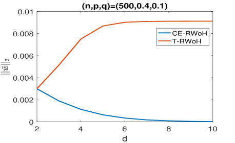
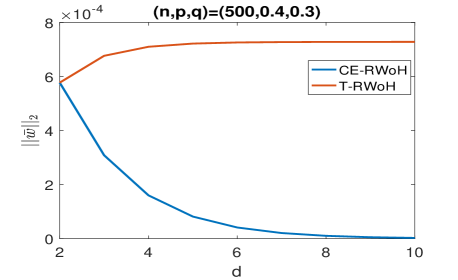
Figure 1: Centroid distances for the two studied RWoHs. We ran $20$ steps of the random walk and used Theorems 3.2, 3.4 to calculate the centroid distance $||\bar{w}||_{2}=\sqrt{\sum_{k=1}^{20}\bar{w}_{k}^{2}}$.

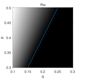
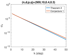
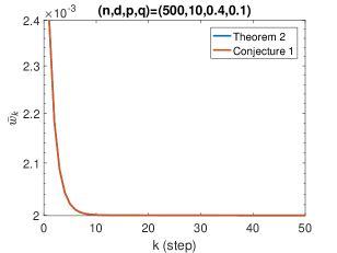
Figure 2: The phase transition following from Theorem 3.4. (Right) The gray scale captures the magnitude of $\bar{w}_{50}$ for different values of $(p,q)$. The darker the shade, the smaller the $\bar{w}_{50}$; the separating line is $p=2q$. (Middle, Left) The decay of $\bar{w}_{k}$ for $(p,q)=(0.4,0.3)$ and $(0.4,0.1)$, respectively.

Although there may not be a general closed form characterization for the centroid distance when $d\geq 6$, we may still obtain some simple approximation results for the case that $d$ is sufficiently large by analyzing the characteristic polynomials of $\beta,\zeta$. For sufficiently large $d$ , we have the following approximation for $\bar{w}_{k}$, $\frac{2}{n}\frac{C_{3}p^{k}}{C_{1}(2q)^{k}+C_{2}p^{k}}$, where $C_{1},C_{2}$ and $C_{3}$ are constants independent of $k$. We describe how this heuristic naturally arises from the characteristic polynomial of the recurrence and how it is supported by extensive simulations in Supplement B.

We also observe that there exists a phase transition at $p=2q$, illustrated in Figure 2. When $p>2q$, we have $\bar{w}_{k}\rightarrow\frac{2}{n}\frac{C_{3}}{C_{2}}$. This implies that the centroid distance does not diminish when increasing the step size $k$. Thus, for this parameter setting the tensor RWoHs behaves fundamentally different from the clique-expansion RWoHs (see Theorem 3.2). On the other hand, if $q<p<2q$ then $\bar{w}_{k}$ decays roughly geometrically similarly to what is proved in Theorem 3.2. We conjecture that the constants are as listed below.

Conjecture 3.1.

$$C_{1}=\frac{-q}{p-2q},\;C_{2}=\frac{p-q}{p-2q},\;C_{3}=\frac{p-q}{p}.$$

Figure 2 also shows that for $p>2q$ the centroid distance decays very slowly with $k$ and that the difference between our conjectured behavior and the result of the pertinent theorem is very small.

The next result shows that the empirical centroids asymptotically concentrate around their mean-fields.

Lemma 3.6.

Assume that $G$ is sampled from a $d$-hSBM$(n,p,q)$ model, for some constant $d\geq 3$. Let the LPs of the tensor RWoHs be $x_{v;t}^{(k)}$ and assume that $\frac{nq^{2}}{\log n}\rightarrow\infty$. For sufficiently large $n$, any constant $\epsilon>0$ and a bounded constant $k$,

$$\frac{2}{n}\left(\sum_{v\in V_{0}}x_{v;t}^{(k)}-\sum_{v\in V_{1}}x_{v;t}^{(k)}\right)$$

$$\in[(1-\epsilon)(\bar{a}^{(k)}-\bar{b}^{(k)}),(1+\epsilon)(\bar{a}^{(k)}-\bar{b}^{(k)})],$$

with probability at least $1-o(1)$.

The proof of Lemma 3.6 is deferred to Supplement E. The above results show that if one sets $\gamma_{k}=\bar{w}_{k}$ in the GPR formulation, it will asymptotically approach the geometric discriminant function or a tight approximation thereof. Independent on the choice of the parameter $\alpha$, the geometric discriminant function of PPR does not match that of the tensor RWoHs on $d$-hSBM. Only the choice of $\gamma_{k}$ suggested by our analysis will allow the aforementioned result to hold true.

4 Proofs

Due to space limitations, we relegate all relevant proofs pertaining to the clique-expansion method to the Supplement and exclusively focus on the tensor case.

The main technical difficulty associated with tensor RWoHs is the large size of the state space, equal to $2^{d-1}$, which makes an analysis akin to the one described in Theorem 3.2 difficult. The main finding of this section is that for the $d$-hSBM, the centroid distances are governed by small recurrences involving only $d-1$ states. The proof supporting this observation comprises two steps, the first step of which is similar to the proof of Theorem 3.2. The second step of the proof describes how to reduce the state space of the recurrence. For simplicity, we start with $d=3$ and then generalize the analysis for arbitrary $d$. For notational convenience, we write $\mathbf{Y}^{(k)}=[Y_{1}^{(k)},Y_{2}^{(k)},Y_{3}^{(k)},Y_{4}^{(k)}]^{T}$.

Theorem 4.1.

Let $G$ be sampled from $3$-hSBM$(n,p,q)$ and let the tensor RWoHs be associated with an initial vector $y^{(0)}_{s_{1},s_{2};t}=1$ and $y^{(0)}_{v_{1},v_{2};t}=0,\;\forall(v_{1},v_{2})\neq(s_{1},s_{2})$, where $s_{1}$ and $s_{2}$ are selected independently and uniformly at random from $V_{0}$. Furthermore, let $\bar{y}^{(0)}_{t}=\mathbb{E}y^{(0)}_{t}$. Then for all $k\geq 0$

$$\bar{y}_{i,j;t}^{(k)}=\begin{cases}Y_{1}^{(k)}&\text{if }(i,j)\in V_{0}\times V_{0},\\ Y_{2}^{(k)}&\text{if }(i,j)\in V_{0}\times V_{1},\\ Y_{3}^{(k)}&\text{if }(i,j)\in V_{1}\times V_{0},\\ Y_{4}^{(k)}&\text{if }(i,j)\in V_{1}\times V_{1},\\ \end{cases}$$ (8)

where $\mathbf{Y}^{(0)}=\frac{4}{n^{2}}[1,0,0,0]^{T}$ and

$$\begin{bmatrix}Y_{1}^{(k+1)}\\ Y_{2}^{(k+1)}\\ Y_{3}^{(k+1)}\\ Y_{4}^{(k+1)}\\ \end{bmatrix}=\begin{bmatrix}\frac{np}{2}&0&\frac{nq}{2}&0\\ \frac{nq}{2}&0&\frac{nq}{2}&0\\ 0&\frac{nq}{2}&0&\frac{nq}{2}\\ 0&\frac{nq}{2}&0&\frac{np}{2}\end{bmatrix}\begin{bmatrix}Y_{1}^{(k)}\\ Y_{2}^{(k)}\\ Y_{3}^{(k)}\\ Y_{4}^{(k)}\end{bmatrix}.$$

Proof.

The proof proceeds by induction: The base case $k=0$ is clearly true. For the induction step, assume that the hypothesis holds for $1,2,...,k$. Then

$$\forall i,j\in V_{0},\;Y_{1}^{(k+1)}=\bar{y}_{i,j;t}^{(k+1)}=\sum_{l=1}^{n}\mathbb{E}A_{lij}\bar{y}_{l,i;t}^{(k)}$$

$$=\sum_{l\in V_{0}}\mathbb{E}A_{lij}\bar{y}_{l,i;t}^{(k)}+\sum_{l\in V_{1}}\mathbb{E}A_{lij}\bar{y}_{l,i;t}^{(k)}$$

$$=\sum_{l\in V_{0}}\mathbb{E}A_{lij}Y_{1}^{(k)}+\sum_{l\in V_{1}}\mathbb{E}A_{lij}Y_{3}^{(k)}=\frac{np}{2}Y_{1}^{(k)}+\frac{nq}{2}Y_{3}^{(k)}.$$

Similar expressions may be derived for $Y_{2}^{(k+1)},Y_{3}^{(k+1)},Y_{4}^{(k+1)}$. This completes the proof. ∎

Next we show how to reduce the number of states to $d-1$. To this end, we simplify $\bar{x}_{i;t}$ as

$$\bar{x}_{j;h}^{(k)}=\frac{\sum_{i=1}^{n}\bar{y}_{i,j;h}^{(k)}}{\sum_{i,l=1}^{n}\bar{y}_{i,l;h}^{(k)}}=\begin{cases}\bar{a}^{(k)}=\frac{2}{n}\frac{Y_{1}^{(k)}+Y_{3}^{(k)}}{\sum_{m=1}^{4}Y_{m}^{(k)}},&\mbox{if }j\in V_{0}\\ \bar{b}^{(k)}=\frac{2}{n}\frac{Y_{2}^{(k)}+Y_{4}^{(k)}}{\sum_{m=1}^{4}Y_{m}^{(k)}},&\mbox{if }j\in V_{1}.\end{cases}$$

The centroid distance $\bar{w}=\bar{a}-\bar{b}$ may be written as

$$\bar{w}_{k}=\bar{a}^{(k)}-\bar{b}^{(k)}=\frac{2}{n}\frac{\beta_{1}(k)}{\zeta_{1}(k)},\text{ where}$$

$$\beta_{1}(k)=[1,-1,1,-1]\mathbf{Y}^{(k)},\,\zeta_{1}(k)=[1,1,1,1]\mathbf{Y}^{(k)}.$$

We introduce next the following auxiliary variables:

$$\beta_{2}(k)=[1,0,0,-1]\mathbf{Y}^{(k)},\,\zeta_{2}(k)=[1,0,0,1]\mathbf{Y}^{(k)}.$$

In the expression for $\beta_{1}(k)$, we replace $\mathbf{Y}^{(k)}$ by $\mathbf{Y}^{(k-1)}$ by invoking the recurrence of Theorem 4.1. One can then show that the recurrence for $\mathbf{Y}^{(k)}$ may be replaced by a recurrence for $\beta_{1}(k)$ and $\beta_{2}(k)$:

$$\begin{bmatrix}\beta_{1}(k+1)\\ \beta_{2}(k+1)\end{bmatrix}=\frac{n}{2}\begin{bmatrix}0&p-q\\ q&p-q\end{bmatrix}\begin{bmatrix}\beta_{1}(k)\\ \beta_{2}(k)\end{bmatrix}.$$ (9)

For $\zeta$, one can derive the following similar result:

$$\begin{bmatrix}\zeta_{1}(k+1)\\ \zeta_{2}(k+1)\end{bmatrix}=\frac{n}{2}\begin{bmatrix}2q&p-q\\ q&p-q\end{bmatrix}\begin{bmatrix}\zeta_{1}(k)\\ \zeta_{2}(k)\end{bmatrix}.$$ (10)

This approach generalizes for arbitrary $d$, but we defer the detailed analysis to Supplement G. Let $e_{i}=[1,0,...,0,-1]$ where there the runlength of zeros equals $2^{i}-2$. Then, $\beta_{i}(k)=[e_{i},e_{i},...,e_{i}]Y^{(k)}$; a similar expression is valid for $\zeta$ with all $-1$s changed to $1$s. As for the case $d=3$, one can establish the following recurrence relations:

$$\begin{bmatrix}\beta_{1}(k)\\ \vdots\\ \beta_{d-1}(k)\end{bmatrix}=\frac{n}{2}\begin{bmatrix}0&\cdots&0&0&p-q\\ q&0&\cdots&0&p-q\\ 0&\ddots&\vdots&0&p-q\\ 0&\cdots&q&0&p-q\\ 0&\cdots&0&q&p-q\\ \end{bmatrix}\begin{bmatrix}\beta_{1}(k-1)\\ \vdots\\ \beta_{d-1}(k-1)\end{bmatrix},$$ (11)

and

$$\begin{bmatrix}\zeta_{1}(k)\\ \vdots\\ \zeta_{d-1}(k)\end{bmatrix}=\frac{n}{2}\begin{bmatrix}2q&\cdots&0&0&p-q\\ q&0&\cdots&0&p-q\\ 0&\ddots&\vdots&0&p-q\\ 0&\cdots&q&0&p-q\\ 0&\cdots&0&q&p-q\\ \end{bmatrix}\begin{bmatrix}\zeta_{1}(c-1)\\ \vdots\\ \zeta_{d-1}(c-1)\end{bmatrix}.$$ (12)

This complete the proof of Theorem 3.4.

5 Construction of GPR based on landing probabilities

In what follows, we use the results of our theoretical results to propose new GPR methods for hypergraph clustering. Following [8], the geometric discriminant of interest equals $w^{T}x_{v},$ where $x_{v}$ is the landing probability vector of the vertex $v$. If only the first moments of the LPs are available, the optimal choice of $w$ corresponding to the maximal marginal separator of the centroids is given in Theorems 3.2 and 3.4 for clique-expansion RWoHs and tensor RWoHs, respectively.

The geometric discriminant only takes the first-order moments of LPs into account. As pointed out in [8], the Fisher discriminant is expected to have better classification performance since it also make use of the covariances of LPs (see Figure 3). More precisely, the Fisher discriminant takes the form $\left(\Sigma^{-1}w\right)^{T}x_{v},$ where $x_{v}$ is the landing probability vector of the vertex $v$ and $\Sigma$ is the covariance matrix of the landing probability vector. The authors of [8] empirically leveraged the information about the second-order moments of LPs. They showed that the Fisher discriminant has a performance that nearly matches that of belief propagation, the statistically optimal method for community detection on SBM [36, 37, 38]. We therefore turn our attention to Fisher discriminant corresponding to clique-expansion and tensor RWoHs.

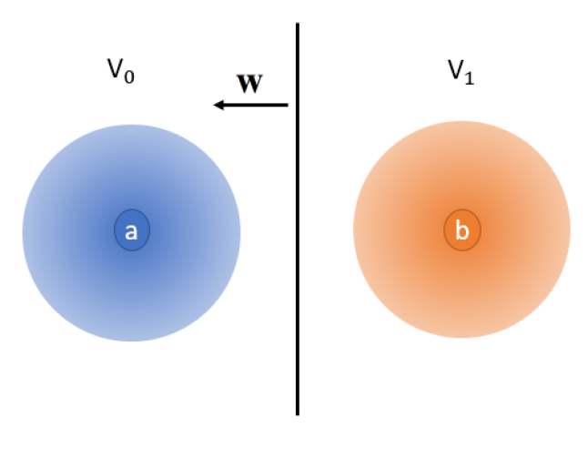
(a) Geometric discriminant.

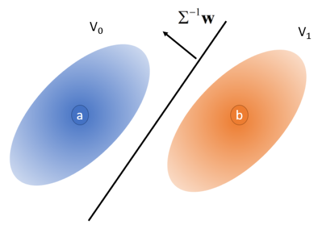
(b) Fisher discriminant.

Figure 3: Illustration of geometric and Fisher discriminants. Consecutive step LPs are correlated as the random walks have memory and one needs to take the covariance into account. The gradations in the colors reflect the density of the LPs in the ambient space.

Recall that our theoretical results shows that tensor RWoHs lead to larger centroid distances compared to those of clique-expansion RWoHs. Most importantly, the difference between the centroid distances of the two methods increase with the hyperedge size $d$. Hence, for large hyperedges sizes the theoretical results suggest that one should not directly use clique-expansion combined with PR methods. On the other hand, clique-expansion leads to reductions in the variance of random walks. This is intuitively clear since entries of the clique-expanded adjacency matrix contain sums of entries of the original adjacency tensor; hence the adjacency matrix obtained through clique-expansion will be “closer” to its expectation, implying a smaller variance. This also follows from Lemma 3.3 and  3.6 by observing that the empirical centroids of clique-expansion RWoHs converge faster as $n$ grows. This points to an important bias-variance trade-off between clique-expansion and tensor RWoHs. We therefore propose the following hybrid random walk scheme combining clique-expansion and tensor methods, referred to “CET RWoHs”. The gist of the CET approach is not to replace a hyperedge by a complete graph as is done in clique-expansion, but replace it by a complete lower order hypergraph instead. On the reduced order hypergraph one can then apply the tensor RWoHs both to increase the centroid distance and to ensure smaller computational and space complexity.

6 Simulations

In the examples that follow, all results are obtained by averaging over $20$ independent trials.

The first test illustrates the clustering performance of geometric and Fisher discriminant corresponding to clique-expansion and tensor RWoHs for $3$-hSBM$(100,p,q)$ with a uniform seed initialization. More precisely, we start with $\bar{y}_{ce}^{(0)}$ and $\bar{y}_{t}^{(0)}$, respectively. Subsequently, we use $k=6$ steps of the random walk for both the clique-expansion RWoHs and tensor RWoHs; our choice is governed by the fact that the centroid distance of the clique-expansion LPs with $k=6$ is close to $0$. Figure 4 shows that for both geometric and Fisher discriminant, using the LPs of tensor RWoHs results in better clustering performance compared to that of clique-expansion RWoHs. This supports our theoretical results.

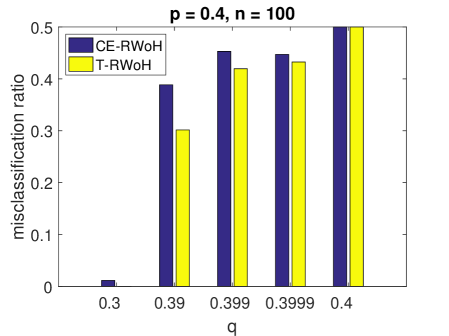
(a) Geometric discriminant.

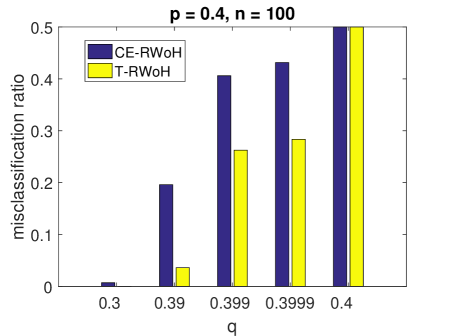
(b) Fisher discriminant.

Figure 4: Clustering performance of the CE (clique-expansion) and T (tensor) methods with uniform initialization on a $3$-hSBM.

However, in practice, one rarely uses a uniform initialization as it implies (partial) prior knowledge of the cluster structure: Seed-set expansion is usually of interest in applications where the seeds are user-defined. To illustrate the performance of the clique-expansion, tensor and CET methods in this setting, we also used single-vertex-seed initializations $y_{ce}^{(0)}$ and $y_{t}^{(0)}$, respectively. Figure 5 provides simulations for a $4$-hSBM$(100,p,q)$, demonstrating that when only the first moment is used (i.e., when the discriminant is geometric), clique-expansion RWoHs offer the best performance. This may be explained by observing that the LPs are correlated and clique-expansion RWoHs has a smaller variance than the other methods. On the other hand, if we additionally use the second moment (i.e., when the discriminant is Fisher), then the CET RWoHs has the best performance in almost all parameter regimes while the tensor RWoHs has the best performance only when $p-q$ is close to $0$. This finding matches our results and their interpretation in Section 5, indicating that CET RWoHs offers good bias-variance trade-offs. As the difference of the centroid distances of clique-expansion and tensor RWoHs grows as the hyperedge size $d$ increases, the performance gain of CET RWoHs is expected to be even larger for higher order hypergraphs. It remains an open question how to choose the best combination of hypergraph projections and tensor RWoHs with respect to both performance and computational complexity.

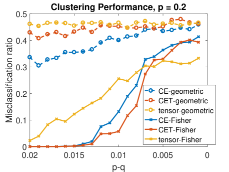
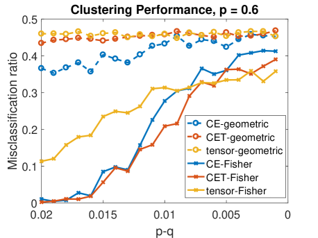
Figure 5: Clustering performance of the CE (clique-expansion), tensor and CET methods with single-seed-vertex initialization on $4$-hSBM.

Acknowledgment: The work was supported by the NSF grant 1956384 and the NSF Center for Science of Information (CSoI) housed at Purdue University.

Appendix A Clique-expansion RWoHs: Proofs

In what follows, we provide a proof of Theorem 3.2.

Recall that $y_{i;ce}^{(k)}$ counts the number of paths of length $k$ starting from some seed vertex $s$ in $G^{(ce)}$ and that $\bar{y}_{i;ce}^{(k)}$ denotes its mean-field complement. Then

$$\forall i\in V_{0},\;\bar{y}^{(1)}_{i;ce} =\frac{2}{n}\sum_{s\in V_{0}}\sum_{v_{1},...,v_{d-2}}\mathbb{E}A_{s,i,v_{1},...,v_{d-2}}$$

$$=\left(\frac{n}{2}\right)^{d-2}(p+(2^{d-2}-1)q);$$

$$\forall i\in V_{1},\;\bar{y}^{(1)}_{i;ce} =\frac{2}{n}\sum_{s\in V_{0}}\sum_{v_{1},...,v_{d-2}}\mathbb{E}A_{s,i,v_{1},...,v_{d-2}}=n^{d-2}q.$$

Let $\bar{F}=\sum_{i\in V}\bar{y}^{(1)}_{i;ce}=\frac{n}{2}((\frac{n}{2})^{d-2}(p+(2^{d-2}-1)q)+n^{d-2}q)=(\frac{n}{2})^{d-1}(p+(2^{d-1}-1)q)$. By definition

$$\forall i\in V_{0},\;\bar{x}^{(1)}_{i;ce} =\frac{1}{\bar{F}}(\frac{n}{2})^{d-2}(p+(2^{d-2}-1)q)$$

$$=\frac{2}{n}\frac{p+(2^{d-2}-1)q}{p+(2^{d-1}-1)q},$$

$$\forall i\in V_{1},\;\bar{x}^{(1)}_{i;ce} =\frac{n^{d-2}q}{\bar{F}}=\frac{2}{n}\frac{2^{d-2}q}{p+(2^{d-1}-1)q}.$$

Based on this one-step analysis and the low-rank structure of the model one may conjecture that for general $k$, $\bar{x}^{(k)}_{v;ce}$ only takes two distinct values depending on $v$. We prove this intuitive observation by induction. Clearly, $\frac{n}{2}[\bar{a}^{(k)}\;\;\bar{b}^{(k)}]^{T}$ is a probability vector and the base case $k=0$ follows directly. For the induction step, assume that the induction hypothesis is true for $1,...,k$. Let $l=(v_{1},...,v_{d-2})$ and write $l\in V$ to indicate that $v_{1},...,v_{d-2}\in V$. Then

$$\forall i\in V_{0},\;\bar{x}^{(k+1)}_{i;ce}=\frac{\bar{y}_{i;ce}^{(k+1)}}{\sum_{j\in V}\bar{y}_{j;ce}^{(k+1)}}=\frac{\sum_{j,l\in V}\mathbb{E}A_{jil}\bar{y}_{j;ce}^{(k)}}{\sum_{j,l,v\in V}\mathbb{E}A_{jvl}\bar{y}_{j;ce}^{(k)}}$$

$$=\frac{\sum_{j,l\in V}\mathbb{E}A_{jil}\bar{x}_{j;ce}^{(k)}}{\sum_{j,l,v\in V}\mathbb{E}A_{jvl}\bar{x}_{j;ce}^{(k)}}$$

$$=\frac{\sum_{j\in V_{0}}\sum_{l}\mathbb{E}A_{jil}\bar{a}^{(k)}+\sum_{j\in V_{1}}\sum_{l}\mathbb{E}A_{jil}\bar{b}^{(k)}}{\sum_{j\in V_{0}}\sum_{l,v}\mathbb{E}A_{jvl}\bar{a}^{(k)}+\sum_{j\in V_{1}}\sum_{l,v}\mathbb{E}A_{jvl}\bar{b}^{(k)}}$$

$$=\frac{(\frac{n}{2})^{d-1}(p+(2^{d-2}-1)q)\bar{a}^{(k)}+\frac{n^{d-1}q}{2}\bar{b}^{(k)}}{\bar{F}\frac{n}{2}(\bar{a}^{(k)}+\bar{b}^{(k)})}=\bar{a}^{(k+1)}.$$

A similar argument may be used to characterize $\bar{b}$.

Appendix B Theorem 3.4: Large $d$ regime

We start by computing the eigenvalues of the update matrix for $\beta$. For this purpose, rewrite (11) as follows:

$$\frac{nq}{2}\times\begin{bmatrix}0&\cdots&0&0&R\\ 1&0&\cdots&0&R\\ 0&\ddots&\vdots&0&R\\ 0&\cdots&1&0&R\\ 0&\cdots&0&1&R\\ \end{bmatrix}\triangleq\frac{nq}{2}\mathbf{Q_{1}},R\triangleq\frac{p-q}{q}.$$ (13)

Note that $\mathbf{Q_{1}}$ takes the form of a companion matrix of dimension $d-1$. It is well known that if $\mathbf{Q_{1}}$ has $d-1$ distinct eigenvalue, then it can be diagonalized as follows

$$UQ_{1}U^{-1}=Diag(\lambda_{1},...,\lambda_{d-1}),$$

where $U$ is the Vandermonde matrix associate with $\lambda_{i}$, and $U_{ij}=\lambda_{i}^{j-i}$. Note that $\mathbf{Q_{1}}$ has full rank when $p>q$.

Next we characterize the eigenvalues $\lambda_{i}$ by writing down the characteristic polynomial of $\mathbf{Q_{1}}$:

$$t^{d-1}=R(t^{d-2}+t^{d-3}+...+1).$$ (14)

In general, there exists no closed form in terms of radicals when $d-1>5$. However, we can find the roots approximately by assuming that $\frac{p-q}{q}=R\neq\frac{1}{d-1}$ and using the following argument. Clearly, $t=1$ is not a root of the polynomial unless $R\triangleq\frac{p-q}{q}=\frac{1}{d-1}$, which we ruled out for the sake of simplifying the analysis. Since we allow $d$ to be large, $R=\frac{1}{d-1}$ implies $p$ will be close to $q$. Also, it is clear that $t=0$ is not a root of the polynomial unless $R=0$. Hence we will also assume that $t\neq 0$. Multiplying both sides of the polynomial expression (14) by $(t-1)$ we obtain

$$t^{d}-(R+1)t^{d-1}+R=0$$

$$\Leftrightarrow t+\frac{R}{t^{d-1}}=R+1.$$ (15)

The eigenvalues of the matrix under consideration satisfy either $|t|>1$ ,$|t|<1$ or $|t|=1$. For $|t|>1$, as $d$ is large, the LHS of (15) will be close to $t$ which implies that there is a root close to $t=R+1>1$. For the case $|t|=1$, we may write $t=e^{i\theta}$. Then $e^{i\theta}+Re^{-i(d-1)\theta}=R+1$. Since $R\in\mathbb{R}$ we require $e^{i\theta}=e^{-i(d-1)\theta}=1$ which violates our assumption that $t=1$ is not a root.

On the other hand, when $|t|<1$, the LHS of (15) has a value close to $\frac{R}{t^{d-1}}$. Thus, the remaining $d-2$ eigenvalues will be close to the $d-1$ complex roots of $t^{d-1}=\frac{R}{R+1}$. However, note that the real root $t=(\frac{R}{R+1})^{1/d}\rightarrow 1$ as $d\rightarrow\infty$ and has to be ruled out. Consequently, we have $\max_{i\in[d-1]}|\lambda_{i}|$ close to $R+1=\frac{p}{q}$ and $|\lambda_{i}|$ close to $(\frac{R}{R+1})^{1/d}=(\frac{p-q}{p})^{1/d}$ for the remaining cases. The numerical results in Figure 6 support our above presented argument.

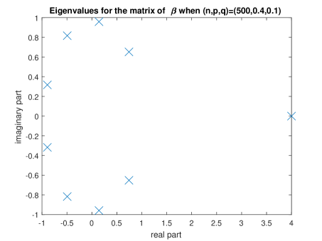
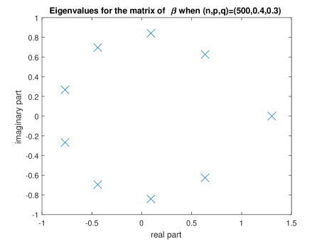
Figure 6: The roots of (14).

Next we evaluate the eigenvalues of the update matrix for $\zeta$, which is a significantly more complicated task. Again we first rewrite the update matrix in (12) as:

$$\frac{nq}{2}\times\begin{bmatrix}2&\cdots&0&0&R\\ 1&0&\cdots&0&R\\ 0&\ddots&\vdots&0&R\\ 0&\cdots&1&0&R\\ 0&\cdots&0&1&R\\ \end{bmatrix}\triangleq\frac{nq}{2}\mathbf{Q_{2}},R\triangleq\frac{p-q}{q}.$$ (16)

Note that we cannot write down a simple explicit formula for of the eigenvalues of $\mathbf{Q_{2}}$ now, as the matrix is not a companion matrix. Still we can show that the characteristic polynomial of $\mathbf{Q_{2}}$ reads as follows

$$t^{d-1}-(2+R)t^{d-2}+R(t^{d-3}+t^{d-4}+...+1)=0.$$ (17)

Similarly, $t=0$ is not a root of the equation since $p>q\Rightarrow R>0$. Moreover, $t=1$ is also not a root unless $R=\frac{1}{d-3}$, which we rule out for simplicity of analysis. Once again multiplying both sides of the equations by $(t-1)$ we have

$$t^{d}-(3+R)t^{d-1}+2(1+R)t^{d-2}=R$$

$$\Leftrightarrow(t-2)(t-(1+R))=\frac{R}{t^{d-2}}.$$ (18)

Obviously, when $|t|>1$ there are two real eigenvalues close to $2$ and $1+R$ whenever $d$ is sufficiently large. On the other hand, the remaining eigenvalues are complex and contained within the ring $\{z\in\mathbb{C}|\;\;|(\frac{R}{2(1+R)})^{\frac{1}{d-1}}|\leq|z|\leq 1\}$. Numerical results also confirm this finding as illustrated in Figure 7.

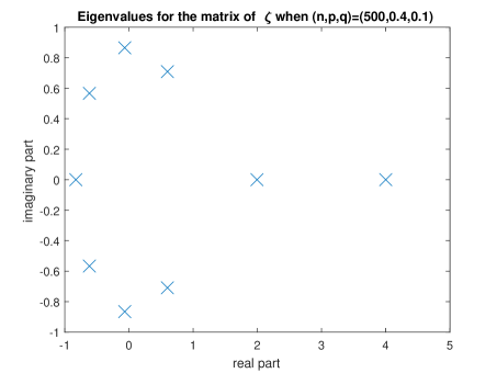
Figure 7: The roots of (17).

Thus by considering only the leading terms in $\beta,\zeta$, $\bar{w}_{k}$ we may write

$$\frac{2}{n}\frac{C_{3}(1+R)^{k}}{C_{1}(2)^{k}+C_{2}(1+R)^{k}}=\frac{2}{n}\frac{C_{3}(p)^{k}}{C_{1}(2q)^{k}+C_{2}(p)^{k}}.$$

Appendix C Closed form results for Theorem 3.4 and $d=3$

When $d=3$, we can have the following closed-form characterization of the centroid distance.

Corollary C.1.

Let $G$ be sampled from a $3$-hSBM$(n,p,q)$ and let the tensor RWoHs be associated with a initial vector $y^{(0)}_{s_{1},s_{2};h}=1$ and $y^{(0)}_{v_{1},v_{2};h}=0,\;\forall(v_{1},v_{2})\neq(s_{1},s_{2})$, where $s_{1}$ and $s_{2}$ are chosen independently and uniformly at random from $V_{0}$. Let $\bar{y}^{(0)}_{h}=\mathbb{E}y^{(0)}_{h}$. Then, the mean-field LPs $\bar{x}_{h}^{k}$ of the tensor RWoHs will have exactly two geometric centroids $\bar{a}^{k},\bar{b}^{k}$ that satisfy

$$\bar{a}^{(k)}-\bar{b}^{(k)}=\frac{2}{n}\frac{\beta_{1}(k)}{\zeta_{1}(k)},$$

where

$$\zeta_{1}(k)=\frac{\sqrt{R^{2}+4}-R-2}{2\sqrt{R^{2}+4}}\times(\frac{nq}{4}(R-\sqrt{R^{2}+4}+2))^{k}$$

$$+\frac{\sqrt{R^{2}+4}+R+2}{2\sqrt{R^{2}+4}}\times(\frac{nq}{4}(R+\sqrt{R^{2}+4}+2))^{k},$$

$$\beta_{1}(k)=\frac{1}{2}\left(1-\sqrt{\frac{R}{R+4}}\right)\times(\frac{nq}{4}(R-\sqrt{R}\sqrt{R+4}))^{k}$$

$$+\frac{1}{2}(1+\sqrt{\frac{R}{R+4}})\times(\frac{nq}{4}(R+\sqrt{R}\sqrt{R+4}))^{k},$$

and $R=\frac{p-q}{p}$.

Corollary C.1 directly follows from the eigenvalue decomposition of the matrices in Theorem 3.4.

Appendix D Proof of Lemma 3.3

The proof follows along the same lines as the proof of the concentration result in [8]. Given $\epsilon>0$ and the fact that $k<K$ for some constant $K$, we choose $\gamma\geq 0$ so that $\left(\frac{1-\gamma}{1+\gamma}\right)^{K}\geq 1-\epsilon$, $\left(\frac{1+\gamma}{1-\gamma}\right)^{K}\leq 1+\epsilon$.

First we set $d_{00}=\mathbb{E}\sum_{u\in V_{0}}A_{vu}^{(ce)},\;v\in V_{0}$; $d_{01},d_{10}$ and $d_{11}$ can be defined similarly. It is not hard to see that under the $d$-hSBM, we have $d_{00}=d_{11}=(\frac{n}{2})^{d-1}(p+(2^{d-2}-1)\times q)$ and $d_{01}=d_{10}=(\frac{n}{2})^{d-1}(2^{d-2}q)$. Next we denote the sum of random variables as following,

$$v\in V_{i},\;S_{ij}\triangleq\sum_{u\in V_{j}}A_{vu}^{(ce)}=\sum_{v_{1},...,v_{d-2}\in V}\sum_{u\in V_{j}}A_{vul}.$$

It is clear that $\mathbb{E}S_{ij}=d_{ij}\geq\frac{n^{d-1}q}{2}$. Then we need to count the number of independent random variables in the above expression for all $i,j\in\{0,1\}$ in order to apply Hoeffding’s bound. Note that the number of independent random variables in summation above is at most

$$\frac{\frac{n^{d-1}}{2}}{\lfloor\frac{d-1}{2}\rfloor!\lceil\frac{d-1}{2}\rceil!},$$

where each of them appears at most $(d-1)!$ times. Hence by Hoeffding’s bound

$$\mathbb{P}\left\{S_{ij}\notin[(1-\gamma)d_{ij},(1+\gamma)d_{ij}]\right\}$$

$$\leq 2\exp\left(-\frac{\lfloor\frac{d-1}{2}\rfloor!\lceil\frac{d-1}{2}\rceil!}{[(d-1)!]^{2}}\gamma^{2}q^{2}n^{d-1}\right),\;\forall i,j\in\{0,1\}.$$

By invoking the union bound over $S_{ij},\forall i,j\in\{0,1\}$ we have

$$\mathbb{P}\left\{S_{ij}\in[(1-\gamma)d_{ij},(1+\gamma)d_{ij}]\right\}$$

$$\geq 1-4n\exp\left(-\frac{\lfloor\frac{d-1}{2}\rfloor!\lceil\frac{d-1}{2}\rceil!}{[(d-1)!]^{2}}\gamma^{2}q^{2}n^{d-1}\right).$$

Hence if $\frac{q^{2}n^{d-1}}{\log(n)}\rightarrow\infty$ then for $d$ constant and $n$ large enough the following event hold

$$S_{ij}\in[(1-\gamma)d_{ij},(1+\gamma)d_{ij}],\;\forall i,j\in\{0,1\}$$ (19)

with probability at least

$$1-4n\exp\left(-\frac{\lfloor\frac{d-1}{2}\rfloor!\lceil\frac{d-1}{2}\rceil!}{[(d-1)!]^{2}}\gamma^{2}q^{2}n^{d-1}\right)=1-o(1).$$

In the derivations that follow we condition our probability computation given this event. We prove by induction that the following two claims are true

$$M^{(k)}\triangleq\sum_{i\in V_{0}}y_{i;ce}^{(k)}\in[(1-\gamma)^{k}\bar{M}^{(k)},(1+\gamma)^{k}\bar{M}^{(k)}]$$

$$N^{(k)}\triangleq\sum_{i\in V_{1}}y_{i;ce}^{(k)}\in[(1-\gamma)^{k}\bar{N}^{(k)},(1+\gamma)^{k}\bar{N}^{(k)}],$$

where $\bar{M},\bar{N}$ satisfy the following recurrence relations

$$\begin{bmatrix}\bar{M}^{(k)}\\ \bar{N}^{(k)}\end{bmatrix}=(\frac{n}{2})^{d-1}\begin{bmatrix}p+(2^{d-2}-1)q&2^{d-2}q\\ 2^{d-2}q&p+(2^{d-2}-1)q\end{bmatrix}\begin{bmatrix}\bar{M}^{(k-1)}\\ \bar{N}^{(k-1)}\end{bmatrix}$$

$$\begin{bmatrix}\bar{M}^{(0)}\\ \bar{N}^{(0)}\end{bmatrix}=\begin{bmatrix}1\\ 0\end{bmatrix}.$$ (20)

The base case holds due to the choice of the initial conditions. For the induction step, by definition we have that $\sum_{i\in V_{0}}y^{(k+1)}_{i;ce}$ equals

$$\sum_{i\in V_{0}}\sum_{j\in V}A^{(ce)}_{ji}y^{(k)}_{j;ce}=\sum_{i\in V_{0}}\sum_{j\in V_{0}}A^{(ce)}_{ji}y^{(k)}_{j;ce}+\sum_{i\in V_{0}}\sum_{j\in V_{1}}A^{(ce)}_{ji}y^{(k)}_{j;ce}$$

$$\leq(1+\gamma)(d_{00}\sum_{j\in V_{0}}y^{(k)}_{j;ce}+d_{10}\sum_{j\in V_{1}}y^{(k)}_{j;ce})$$

$$\leq(1+\gamma)^{k+1}(d_{00}\bar{M}^{(k)}+d_{10}\bar{N}^{(k)})$$

$$\leq(1+\gamma)^{k+1}\bar{M}^{(k+1)}$$

Similar arguments may be used for the lower bound and for $N$. Hence, by the definition of $x_{ce}$ we have

$$\frac{2}{n}\sum_{i\in V_{0}}x_{i;ce}^{(k)}\in\left[\frac{(1-\gamma)^{k}}{(1+\gamma)^{k}}\frac{2}{n}\frac{\bar{M}^{(k)}}{\bar{M}^{(k)}+\bar{N}^{(k)}},\frac{(1+\gamma)^{k}}{(1-\gamma)^{k}}\frac{2}{n}\frac{\bar{M}^{(k)}}{\bar{M}^{(k)}+\bar{N}^{(k)}}\right]$$

$$\frac{2}{n}\sum_{i\in V_{1}}x_{i;ce}^{(k)}\in\left[\frac{(1-\gamma)^{k}}{(1+\gamma)^{k}}\frac{2}{n}\frac{\bar{N}^{(k)}}{\bar{M}^{(k)}+\bar{N}^{(k)}},\frac{(1+\gamma)^{k}}{(1-\gamma)^{k}}\frac{2}{n}\frac{\bar{N}^{(k)}}{\bar{M}^{(k)}+\bar{N}^{(k)}}\right].$$

Based on our choice of $\gamma$, and the assumption that $\forall k\leq K$ we also have

$$\frac{2}{n}\sum_{i\in V_{0}}x_{i;ce}^{(k)}\in\left[(1-\epsilon)\frac{2}{n}\frac{\bar{M}^{(k)}}{\bar{M}^{(k)}+\bar{N}^{(k)}},(1+\epsilon)\frac{2}{n}\frac{\bar{M}^{(k)}}{\bar{M}^{(k)}+\bar{N}^{(k)}}\right]$$

$$\frac{2}{n}\sum_{i\in V_{1}}x_{i;ce}^{(k)}\in\left[(1-\epsilon)\frac{2}{n}\frac{\bar{N}^{(k)}}{\bar{M}^{(k)}+\bar{N}^{(k)}},(1+\epsilon)\frac{2}{n}\frac{\bar{N}^{(k)}}{\bar{M}^{(k)}+\bar{N}^{(k)}}\right].$$

Hence it remains to show that

$$\bar{a}^{(k)}=\frac{2}{n}\frac{\bar{M}^{(k)}}{\bar{M}^{(k)}+\bar{N}^{(k)}}$$

and

$$\bar{b}^{(k)}=\frac{2}{n}\frac{\bar{N}^{(k)}}{\bar{M}^{(k)}+\bar{N}^{(k)}}.$$

First, observe that

$$\bar{M}^{(k)}+\bar{N}^{(k)}=[1,1][\bar{M}^{(k)},\bar{N}^{(k)}]^{T}$$ (21)

$$=(\frac{n}{2})^{d-1}(p+(2^{d-1}-1)q)(\bar{M}^{(k-1)}+\bar{N}^{(k-1)}).$$

Replacing (21) into (D) we obtain the claimed recurrence relation for $\bar{a}$, $\bar{b}$. Given that the initial conditions agree, the result follows.

Appendix E Proof of Lemma 3.6

The proof is almost identical to the proof of Lemma 3.3. We first prove the concentration of $\sum_{l}A_{v_{1},...,v_{d-1},l}$. Then, the second half of the proof is the same as the second half of the proof of Lemma 3.3, provided that one modifies the arguments according to the tensor update rule (described in Section 4). For simplicity we therefore only focus on the first half of the proof. As before, define $d_{0...0}=\mathbb{E}\sum_{l\in V_{0}}A_{v_{1},...,v_{d-1},l},v_{1},...,v_{d-1}\in V_{0}$ and all the other $d$ similarly. Note that $d_{0...0}=d_{1...1}=\frac{n}{2}p$ and that the remaining $d$ take the value $\frac{n}{2}q$. By Hoeffding’s bound we have for $v_{1},...,v_{d-1}\in V_{0}$,

$$\mathbf{P}\left\{\sum_{l\in V_{0}}A_{v_{1},...,v_{d-1}l}\notin[(1-\gamma)d_{0...0},(1+\gamma)d_{0...0}]\right\}$$

$$\leq 2\exp(-np^{2}\gamma^{2}).$$

Similarly, for $v_{1},...,v_{d-1}\in V_{0}$,

$$\mathbf{P}\left\{\sum_{l\in V_{1}}A_{v_{1},...,v_{d-1},l}\notin[(1-\gamma)d_{0...01},(1+\gamma)d_{0...01}]\right\}$$

$$\leq 2\exp(-nq^{2}\gamma^{2}).$$

From the union bound over all possible $v_{1},...,v_{d-1}$ and the community of $l$, we have $\forall r\in\{0,1\}$

$$\mathbf{P}\Bigg{\{}\sum_{l\in V_{r}}A_{v_{1},...,v_{d-1},l}$$

$$\notin[(1-\gamma)d_{\sigma(v_{1})...\sigma(v_{d-1})r},(1+\gamma)d_{\sigma(v_{1})...\sigma(v_{d-1})r}]\Bigg{\}}$$

$$\leq 4n^{d-1}\exp(-nq^{2}\gamma^{2}),$$

where we denote $\sigma(v_{i})$ to be the community of vertex $v_{i}$. Therefore, if $\frac{nq^{2}}{\log(n)}\rightarrow\infty$, then for $n$ sufficiently large with high probability we have $\forall v_{1},...,v_{d-1},\;\forall r\in\{0,1\}$,

$$\sum_{l\in V_{r}}A_{v_{1},...,v_{d-1},l}\in[(1-\gamma)d_{\sigma(v_{1})...\sigma(v_{d-1})r},(1+\gamma)d_{\sigma(v_{1})...\sigma(v_{d-1})r}],$$

with probability at least $1-4n^{d-1}\exp(-nq^{2}\gamma^{2})=1-o(1)$. This completes the proof.

Appendix F Proof of Theorem 3.5

From Theorem 3.4, one can see that the characteristic function of $\beta$ equals

$$t^{d-1}=R(t^{d-2}+\cdots+1),$$

and the characteristic function of $\zeta$ equals

$$t^{d-1}=(2+R)t^{d-2}-R(t^{d-3}+\cdots+1),$$

where $R=\frac{p-q}{q}$. Hence $\beta_{1}$ and $\zeta_{1}$ satisfy

$$\beta_{1}(k) =R(\beta_{1}(k-1)+\cdots+\beta_{1}(k-(d-1)))$$

$$\zeta_{1}(k) =(2+R)\zeta_{1}(k-1)$$

$$-R(\beta_{1}(k-2)+\cdots+\beta_{1}(k-(d-1))).$$

Moreover, from the initial condition in Theorem 3.4 we can easily observe that $\forall k\geq 0$, $\beta_{1}(k)\geq 0$ and $\zeta_{1}(k)\geq 0$. The proof then follows from

$$\bar{w}_{k}=\frac{2}{n}\frac{\beta_{1}(k)}{\zeta_{1}(k)}$$

$$=\frac{2}{n}\frac{R(\beta_{1}(k-1)+\cdots+\beta_{1}(k-(d-1)))}{(2+R)\zeta_{1}(k-1)-R(\beta_{1}(k-2)+\cdots+\beta_{1}(k-(d-1)))}$$

$$\geq\frac{2}{n}\frac{\beta_{1}(k-1)}{\zeta_{1}(k-1)}\frac{R}{R+2}=\frac{R}{R+2}\bar{w}_{k-1}=\frac{p-q}{p+q}\bar{w}_{k-1}.$$

Appendix G Remaining proof of Theorem 3.4

Let $(i)^{d-1}$ be the binary representation of $i$ of length $d-1$ and let $(i)^{d-1}[j]$ be the $j^{th}$ bit from the right in this representation (i.e. $(3)^{4}=0011$ and $(3)^{4}[3]=0$). For arbitrary $d,$ we have $\bar{y}_{v_{1},...,v_{d-1};h}=Y_{j}$ if $v_{i}\in V_{(j-1)^{d-1}[i]}$. It is clear that $Y_{j_{1}}^{(k)}$ depends only on $Y_{j_{2}}^{(k-1)}$ and $Y_{j_{3}}^{(k-1)}$ where $(j_{2}-1)^{d-1}[1:d-2]=(j_{2}-1)^{d-1}[2:d-1]=(j_{3}-1)^{d-1}[2:d-1]$ (i.e. state $001$ is determined by $100$ and $000$). By the similar analysis as the $d=3$ case, the recurrence relations becomes:

$$\begin{bmatrix}Y_{1}^{(k+1)}\\ \vdots\\ Y_{2^{d-1}}^{(k+1)}\end{bmatrix}=\begin{bmatrix}\frac{np}{2}&0&\cdots&\frac{nq}{2}&0&\cdots&0\\ \frac{nq}{2}&0&\cdots&\frac{nq}{2}&0&\cdots&0\\ 0&\frac{nq}{2}&0&\cdots&\frac{nq}{2}&0&\cdots&0\\ 0&\frac{nq}{2}&0&\cdots&\frac{nq}{2}&0&\cdots&0\\ &&&&\vdots\\ 0&\cdots&\frac{nq}{2}&0&\cdots&\frac{nq}{2}\\ 0&\cdots&\frac{nq}{2}&0&\cdots&\frac{np}{2}\end{bmatrix}\begin{bmatrix}Y_{1}^{(k)}\\ \vdots\\ Y_{2^{d-1}}^{(k)}\end{bmatrix},$$

$$\begin{bmatrix}Y_{1}^{(0)}\\ \vdots\\ Y_{2^{d-1}}^{(0)}\end{bmatrix}=\frac{2^{d-1}}{n^{d-1}}\begin{bmatrix}1\\ 0\\ \vdots\\ 0\end{bmatrix}$$

Applying these recurrence relations with the definition of $\beta,\zeta$ completes the proof.

References

- [1] L. Lovász et al., “Random walks on graphs: A survey,” Combinatorics, Paul Erdös is eighty, vol. 2, no. 1, pp. 1–46, 1993.
- [2] L. Page, S. Brin, R. Motwani, and T. Winograd, “The pagerank citation ranking: Bringing order to the web.” Stanford InfoLab, Tech. Rep., 1999.
- [3] X. Zhu and Z. Ghahramani, “Learning from labeled and unlabeled data with label propagation,” Citeseer, Tech. Rep., 2002.
- [4] R. Andersen, F. Chung, and K. Lang, “Local graph partitioning using pagerank vectors,” in 2006 47th Annual IEEE Symposium on Foundations of Computer Science (FOCS’06). IEEE, 2006, pp. 475–486.
- [5] D. F. Gleich and C. Seshadhri, “Vertex neighborhoods, low conductance cuts, and good seeds for local community methods,” in Proceedings of the 18th ACM SIGKDD international conference on Knowledge discovery and data mining. ACM, 2012, pp. 597–605.
- [6] U. Von Luxburg, A. Radl, and M. Hein, “Hitting and commute times in large random neighborhood graphs,” The Journal of Machine Learning Research, vol. 15, no. 1, pp. 1751–1798, 2014.
- [7] D. Aldous and J. Fill, “Reversible markov chains and random walks on graphs,” 1995.
- [8] I. M. Kloumann, J. Ugander, and J. Kleinberg, “Block models and personalized pagerank,” Proceedings of the National Academy of Sciences, vol. 114, no. 1, pp. 33–38, 2017.
- [9] F. Chung, “The heat kernel as the pagerank of a graph,” Proceedings of the National Academy of Sciences, vol. 104, no. 50, pp. 19 735–19 740, 2007.
- [10] P. W. Holland, K. B. Laskey, and S. Leinhardt, “Stochastic blockmodels: First steps,” Social networks, vol. 5, no. 2, pp. 109–137, 1983.
- [11] S. Agarwal, J. Lim, L. Zelnik-Manor, P. Perona, D. Kriegman, and S. Belongie, “Beyond pairwise clustering,” in 2005 IEEE Computer Society Conference on Computer Vision and Pattern Recognition (CVPR’05), vol. 2. IEEE, 2005, pp. 838–845.
- [12] A. R. Benson, D. F. Gleich, and J. Leskovec, “Higher-order organization of complex networks,” Science, vol. 353, no. 6295, pp. 163–166, 2016.
- [13] P. Li, H. Dau, G. Puleo, and O. Milenkovic, “Motif clustering and overlapping clustering for social network analysis,” in IEEE INFOCOM 2017-IEEE Conference on Computer Communications. IEEE, 2017, pp. 1–9.
- [14] P. Li and O. Milenkovic, “Inhomogeneous hypergraph clustering with applications,” in Advances in Neural Information Processing Systems, 2017, pp. 2308–2318.
- [15] C. Yang, Y. Feng, P. Li, Y. Shi, and J. Han, “Meta-graph based hin spectral embedding: Methods, analyses, and insights,” in 2018 IEEE International Conference on Data Mining (ICDM). IEEE, 2018, pp. 657–666.
- [16] D. Zhou, J. Huang, and B. Schölkopf, “Learning with hypergraphs: Clustering, classification, and embedding,” in Advances in Neural Information Processing Systems, 2007, pp. 1601–1608.
- [17] U. Chitra and B. Raphael, “Random walks on hypergraphs with edge-dependent vertex weights,” in International Conference on Machine Learning, 2019, pp. 1172–1181.
- [18] H. Yin, A. R. Benson, J. Leskovec, and D. F. Gleich, “Local higher-order graph clustering,” in Proceedings of the 23rd ACM SIGKDD International Conference on Knowledge Discovery and Data Mining. ACM, 2017, pp. 555–564.
- [19] M. Hein, S. Setzer, L. Jost, and S. S. Rangapuram, “The total variation on hypergraphs-learning on hypergraphs revisited,” in Advances in Neural Information Processing Systems, 2013, pp. 2427–2435.
- [20] P. Li, N. He, and O. Milenkovic, “Quadratic decomposable submodular function minimization,” in Advances in Neural Information Processing Systems, 2018, pp. 1062–1072.
- [21] I. E. Chien, H. Zhou, and P. Li, “: Active learning over hypergraphs with pointwise and pairwise queries,” in The 22nd International Conference on Artificial Intelligence and Statistics, 2019, pp. 2466–2475.
- [22] T. Wu, A. R. Benson, and D. F. Gleich, “General tensor spectral co-clustering for higher-order data,” in Advances in Neural Information Processing Systems, 2016, pp. 2559–2567.
- [23] T.-H. H. Chan, A. Louis, Z. G. Tang, and C. Zhang, “Spectral properties of hypergraph laplacian and approximation algorithms,” Journal of the ACM (JACM), vol. 65, no. 3, p. 15, 2018.
- [24] D. Ghoshdastidar, A. Dukkipati et al., “Consistency of spectral hypergraph partitioning under planted partition model,” The Annals of Statistics, vol. 45, no. 1, pp. 289–315, 2017.
- [25] I. Chien, C.-Y. Lin, and I.-H. Wang, “Community detection in hypergraphs: Optimal statistical limit and efficient algorithms,” in International Conference on Artificial Intelligence and Statistics, 2018, pp. 871–879.
- [26] K. Ahn, K. Lee, and C. Suh, “Hypergraph spectral clustering in the weighted stochastic block model,” IEEE Journal of Selected Topics in Signal Processing, vol. 12, no. 5, pp. 959–974, 2018.
- [27] I. Chien, C.-Y. Lin, and I.-H. Wang, “On the minimax misclassification ratio of hypergraph community detection,” IEEE Transactions on Information Theory, 2019.
- [28] P. Li, E. Chien, and O. Milenkovic, “Optimizing generalized pagerank methods for seed-expansion community detection,” Advances in Neural Information Processing Systems, 2019.
- [29] D. F. Gleich, L.-H. Lim, and Y. Yu, “Multilinear pagerank,” SIAM Journal on Matrix Analysis and Applications, vol. 36, no. 4, pp. 1507–1541, 2015.
- [30] A. R. Benson, D. F. Gleich, and L.-H. Lim, “The spacey random walk: A stochastic process for higher-order data,” SIAM Review, vol. 59, no. 2, pp. 321–345, 2017.
- [31] J. Xie, S. Kelley, and B. K. Szymanski, “Overlapping community detection in networks: The state-of-the-art and comparative study,” Acm computing surveys (csur), vol. 45, no. 4, p. 43, 2013.
- [32] S. Paul, O. Milenkovic, and Y. Chen, “Higher-order spectral clustering under superimposed stochastic block model,” arXiv preprint arXiv:1812.06515, 2018.
- [33] M. C. Angelini, F. Caltagirone, F. Krzakala, and L. Zdeborová, “Spectral detection on sparse hypergraphs,” in 2015 53rd Annual Allerton Conference on Communication, Control, and Computing (Allerton). IEEE, 2015, pp. 66–73.
- [34] C. Kim, A. S. Bandeira, and M. X. Goemans, “Stochastic block model for hypergraphs: Statistical limits and a semidefinite programming approach,” arXiv preprint arXiv:1807.02884, 2018.
- [35] N. H. Abel, Mémoire sur les équations algébrique: où on démontre l’impossiblité de la résolution de l’equation générale du cinquième dégré. Librarian, Faculty of Science, University of Oslo, 1824.
- [36] E. Abbe and C. Sandon, “Detection in the stochastic block model with multiple clusters: proof of the achievability conjectures, acyclic bp, and the information-computation gap,” arXiv preprint arXiv:1512.09080, 2015.
- [37] P. Zhang and C. Moore, “Scalable detection of statistically significant communities and hierarchies, using message passing for modularity,” Proceedings of the National Academy of Sciences, vol. 111, no. 51, pp. 18 144–18 149, 2014.
- [38] E. Mossel, J. Neeman, and A. Sly, “Belief propagation, robust reconstruction and optimal recovery of block models,” in Conference on Learning Theory, 2014, pp. 356–370.