Testing the Spectroscopic Extraction of Suppression of Convective Blueshift

Abstract

Efforts to detect low-mass exoplanets using stellar radial velocities (RVs) are currently limited by magnetic photospheric activity. Suppression of convective blueshift is the dominant magnetic contribution to RV variability in low-activity Sun-like stars. Due to convective plasma motions, the magnitude of RV contributions from the suppression of convective blueshift is related to the depth of formation of photospheric spectral lines of a given species used to compute the RV time series. Meunier et al. (2017a, b), used this relation to demonstrate a method for spectroscopic extraction of the suppression of convective blueshift in order to isolate RV contributions, including planetary RVs, that contribute equally to the timeseries for each spectral line. Here, we extract disk-integrated solar RVs from observations over a 2.5 year time span made with the solar telescope integrated with the HARPS-N spectrograph at the Telescopio Nazionale Galileo (La Palma, Canary Islands, Spain). We apply the methods outlined by Meunier et al. (2017a, b). We are not, however, able to isolate physically meaningful contributions of the suppression of convective blueshift from this solar dataset, potentially because our dataset is from solar minimum when the suppression of convective blueshift may not sufficiently dominate activity contributions to RVs. This result indicates that, for low-activity Sun-like stars, one must include additional RV contributions from activity sources not considered in the Meunier et al. 2017 model at different timescales as well as instrumental variation in order to reach the sub-meter per second RV sensitivity necessary to detect low-mass planets in orbit around Sun-like stars.

1 Introduction

The radial velocity (RV) method is the principal technique for constraining the masses of exoplanets (Mayor & Queloz, 1995). It provides complementary information to the transit method, e.g., as used by the Kepler and TESS spacecraft (Borucki et al., 2010; Howell et al., 2014; Ricker et al., 2014) and ground-based transit surveys. The Keplerian reflex motion induced in a Sun-like star by an Earth-mass planet in the habitable zone is of order 10 cm s^-1 (Fischer et al., 2016), the target sensitivity of next-generation spectrographs (Pepe et al., 2010). However, contributions to observed stellar RVs from photospheric stellar activity often exceed 1 m s^-1 even in the quietest Sun-like stars, posing a significant barrier to the detection of exoplanets by the RV method (e.g. Saar & Donahue 1997; Schrijver & Zwaan 2000; Isaacson & Fischer 2010; Motalebi et al. 2015). Several recent works describe a variety of models to mitigate the effects of magnetic activity on stellar RVs. One approach has been to study the Sun as a star, extracting solar activity estimates from images of the solar surface (Meunier et al., 2010a; Haywood et al., 2016; Milbourne et al., 2019) and comparing to simultaneous disk-integrated spectral measurements. In order to reduce unwanted stellar signals from exoplanet searches, however, methods for extracting stellar activity directly from spectra, and not from ancillary datasets, must be developed.

For Sun-like stars with low activity, suppression of convective blueshift due to photospheric plage (hereafter $\rm RV_{\rm conv}$) dominates over the wavelength-independent photometric effects due to spots, or RV shifts induced by Earth-like exoplanets (Meunier et al., 2010b; Dumusque et al., 2014; Haywood et al., 2016) (hereafter $\rm RV_{\rm sppl}$). Meunier et al. (2017a) (hereafter M17) have developed one model to isolate $\rm RV_{\rm conv}$ contributions based on the observed non-linear relationship between relative depths and absolute RV blueshifts of spectral lines of a given species (here neutral iron) driven by plasma flow in granules, as described in Gray (2009); Reiners et al. (2016); Meunier et al. (2017b); Gray & Oostra (2018). The exact physical origin of this observed correlation is non-trivial: a correct description of spectral line formation necessitates the summation of many different line profiles, each formed at different depths in the photosphere, and requires a full three-dimensional treatment (e.g., see Nordlund et al. 2009; Stein 2012; Cegla et al. 2013; Bergemann et al. 2019 and references therein). An intuitive (though inexact) understanding of this relationship may be determined by considering a simplified 1D picture: in this model, rising plasma low in the photosphere exhibits strong RV blueshift, while plasma closer to the surface has most of its motion directed tangentially as it merges into intergranular lanes, thus exhibiting less RV blueshift (Dravins et al., 1981). While many factors such as temperature, electron pressure, and atomic constants affect spectral line relative depth (Gray, 2005), for spectral lines of a given atomic species, line depth shows strong anti-correlation with height of formation in the stellar photosphere. Therefore, the absolute radial velocity blueshift shows a strong, non-linear relationship with line depth, commonly referred to as the third signature of stellar granulation (Gray, 2009). M17 leverage the dominance of $\rm RV_{\rm conv}$ to write the RV time series derived from a set of lines $s_{0}$ as

$$\rm RV_{0}=\rm RV_{\rm sppl}+\rm RV_{\rm conv}$$ (1)

where RV₀ is the radial velocity measured with this specific line list. $\rm RV_{\rm conv}$ are line-list dependent contributions due to the suppression of convective blueshift, and $\rm RV_{\rm sppl}$ are photometric variations (e.g. spots and plage), planetary signals, or other RV sources that are the same for all spectral lines.

M17 makes use of the non-linear relationship between line depth and convective shift by writing an an RV time series from a sublist $s_{1}$ of $s_{0}$ with a restricted flux range can be written

$$\rm RV_{1}=\rm RV_{\rm sppl}+\alpha\rm RV_{\rm conv}$$ (2)

where $\alpha$ is the ratio of the weighted mean shift in radial velocity by suppression of convective blueshift from line list $s_{1}$ compared to line list $s_{0}$. Based on the third signature of granulation (Gray, 2009), we would expect $\alpha<1$ for a sublist $s_{1}$ comprising strong lines formed close to the top of the photosphere, and $\alpha>1$ for a sublist of weak lines, formed deep in the photosphere. If a precise value for $\alpha$ is known or can be inferred, we can invert the observed $RV_{0}$ and $RV_{1}$ time series to extract time series of interest $RV_{\rm conv}$ and $RV_{\rm sppl}$.

Using time series $\rm RV_{\rm conv}$ and $\rm RV_{\rm sppl}$ extracted from solar photospheric images, M17 construct synthetic time series $\rm RV_{0}$ and $\rm RV_{1}$ using a value for $\alpha$ fitted from a solar atlas (Kurucz et al., 1984; Kurucz, 2005) and added white noise. The authors then test several methods for estimating $\alpha$ on these synthetic time series, finding good convergence for the value of $\alpha$ across the methods (within 5% of the true value for low-noise conditions) (M17). Using this calculated value of $\alpha$, they then recover and validate the original $\rm RV_{\rm sppl}$ time series. Ideally, this technique could be utilized to correct RV time series for $\rm RV_{\rm conv}$ contributions to lower the RV activity threshold.

On real data, determining an absolute scale for radial velocities is challenging, making it difficult to precisely determine $\alpha$. M17 apply these methods to HARPS exposures of HD207129 but find no agreement for values of $\alpha$ derived by different estimation methods, which they attribute to infrequent observations and low SNR.

Using the solar telescope (Phillips et al., 2016) operating with the HARPS-N spectrograph at the Telescopio Nazionale Galileo (TNG, Cosentino et al. 2012), we extract high-resolution disk-integrated solar spectra (Dumusque et al., 2015). We now have more than 50,000 high-SNR solar exposures spanning over 4 years of observing (Collier Cameron et al., 2019). In this work, we apply Meunier’s methods to the first 2.5 years of the solar dataset (from Summer 2015 - November 2017) to attempt a recovery of a precise value of $\alpha$ for use in reconstructing $\rm RV_{\rm conv}$ and $\rm RV_{\rm sppl}$. In Section 2, we discuss our method for extracting line-by-line RVs from the HARPS-N solar spectra. In Section 3, we discuss various techniques for determining $\alpha$ from the resulting RV timeseries, and attempt to compute consistent $\alpha$ values. We conclude in Section 4 with a discussion of the resulting values, and possible explanations for why the model does not reduce RV RMS on our dataset

2 Methods

2.1 Extracting RVs from HARPS-N spectra

Third signature plots in the literature are often based on neutral iron lines to demonstrate the relationship between relative depth and absolute convective blueshift (Gray, 2009; Reiners et al., 2016; Gray & Oostra, 2018). In order to compare lines known to exhibit the third signature effect, we consider a line list from the NIST database for Fe I lines. We extract disk-integrated HARPS-N solar spectra over a 2.5 year span, with an average of 51 exposures per day. We cut data taken in overcast weather, as identified using the HARPS-N exposure meter, and reject data for any day with five or fewer exposures. Each spectrum is shifted to a heliocentric reference frame using relative velocities from the JPL Horizons ephemeris (Giorgini et al., 1996). We normalize the spectrum continuum by dividing by the corresponding blaze measurement - we propagate the photon shot noise error from each into the fits of each spectral line, as described below.

Table 1: First ten iron line uses in this analysis. An extended line list containing all 765 spectral lines used in out analysis is available online at DOI:https://doi.org/10.5281/zenodo.3541149 (catalog 10.5281/zenodo.3541149).

Wavelength (Å)
3922.91
3946.99
3948.10
3975.21
3995.98
4000.25
4000.46
4001.66
4022.74
4047.30
⋮

For each individual spectral line, we stack the Doppler-shifted measurements from a given day to produce a composite line profile for each day. This approach, stacking data from different exposures instead of averaging over multiple exposures, avoids interpolating data onto a common wavelength grid. We fit the line core (0.2 Angstroms total) with Gaussian profiles to extract relative depth, and line center (0.1 Angstroms total) with 2nd-degree polynomials to measure the RV. We adopted polynomial fits to best mirror the methods of M17. We then convert these line center positions from wavelength to RV. This process is illustrated in Figure 1. Removing poorly-fit and blended lines results in a final list of 765 spectral lines, given in Table 1.

The relative velocities derived reproduce the shape of the third signature curve from Reiners et al. (2016) up to an overall offset, as shown in Figure 2. This offset may result from differences between the line lists or instruments used.

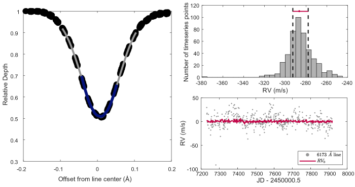
Figure 1: Left: Illustration of boundaries of observed points (black) included in fits for Gaussian (gray curve) and polynomial (dark blue curve) fits for a representative line (at 6173 Å). Right, top: demonstration of zeroing procedure for same 6173 Å line– the average of the middle two quartiles of RV values per line is subtracted off. Right, bottom: zeroed RV time series for 6173 Å line (gray), compared to average time series for all lines, $RV_{0}$ (red).

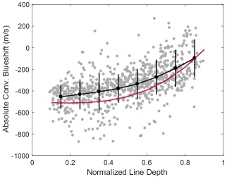
Figure 2: Third signature of stellar granulation trend demonstrated in Fe I list extracted from NIST database. Lines are binned in 0.1 relative depth bins: black dots show the average value per bin, and errorbars show standard deviation per bin. The red curve shows the polynomial of best fit from Reiners et al. (2016).

2.2 Zeroing RV time series

It is challenging to extract absolute RVs from spectral data. In accounting for blueshifts of individual spectral lines, we must identify the hypothetical RV value achieved in the absence of stellar activity, which will vary from line to line, in a manner that is robust against outlier points or noise. We zero the radial velocity time series per spectral line to account for this absolute blueshift. We sort time series observations by RV value per line, and subtract the average of the middle two quartiles, as shown in Figure 1. In selecting this range, we assume that low-activity days will fall close to the median value; by subtracting the average value for the low-activity days, we aim to identify the hypothetical no-activity point for each line while avoiding bias in our zero point due to outliers.

2.3 Finding RVs from sublists

Following the procedure of M17, we identify line sublists by relative depth. We take variance-weighted means of the entire line list ($s_{0}$), lines with relative depth .5-.95 ($s_{1}$), and lines with relative depth .05-.5 ($s_{2}$), to extract $\rm RV_{0}$, $\rm RV_{1}$, and $\rm RV_{2}$ respectively. The RV errors are computed from fit errorbars on the line center parameter, which incorporate propagated shot noise from the raw spectra. Features of these time series are listed in Table 2, while the time series themselves are given in Table 3.

Table 2: Features of RV time series extracted from HARPS-N/solar telescope daily binned spectra.

	$\rm RV_{0}$	$\rm RV_{1}$	$\rm RV_{2}$
Relative Depth	.05-.95	.5-.95	.05-.5
Number of Lines	765	386	379
Standard Deviation (m s-1)	1.50	1.64	1.74
Mean (m s-1)	.47	.37	.59

Table 3: The extracted time series $\rm RV_{0}$, $\rm RV_{1}$, and $\rm RV_{2}$ used in this analysis. The RVs derived from the HARPS-N DRS ($\rm RV_{DRS}$) are also provided as a point of comparison. The first ten RV values are given here - an extended list containing all values is available at DOI:https://doi.org/10.5281/zenodo.3541149 (catalog 10.5281/zenodo.3541149).

JD - 2450000.5	$\rm RV_{0}$ (m s-1)	$\rm RV_{1}$ (m s-1)	$\rm RV_{2}$ (m s-1)	$\rm RV_{drs}$ (m s-1)
7232.51	1.34	1.26	1.46	5.66
7233.54	2.00	2.15	1.81	6.71
7234.51	0.96	-0.16	2.38	6.24
7235.49	0.99	0.06	2.15	6.89
7236.51	1.13	-0.34	2.99	7.48
7237.49	1.79	0.68	3.19	7.12
7238.56	0.59	-0.32	1.75	5.25
7239.43	-0.70	-1.46	0.25	5.38
7241.55	1.00	0.07	2.18	5.34
7244.47	-1.08	-2.58	0.82	2.31
⋮	⋮	⋮	⋮	⋮

To validate our extracted time series, we compare to the HARPS-N Data Reduction System (DRS) RVs (Baranne et al., 1996; Sosnowska et al., 2012). Figure 3 shows a Lomb-Scargle periodogram comparison of the two time series (Zechmeister & Kürster, 2009; VanderPlas et al., 2012; VanderPlas & Ivezić, 2015). Many of the periods with highest concentration of signal power align between the two series, suggesting that they capture the same solar physics. We note that the power concentrated at rotation and half-rotation periods in $\rm RV_{1}$ exceeds that of $\rm RV_{2}$, normalizing to the false alarm probability (FAP). While the RMS scatter of $\rm RV_{2}$ is greater than $\rm RV_{1}$, we find that over 1.5 $\rm ms^{-1}$ of white noise would need to be added to $\rm RV_{2}$ compared to $\rm RV_{1}$ to account for this difference in peak heights. The model from M17 would predict, however, that since $\rm RV_{2}$ is calculated from lines presumably formed lower in the stellar photosphere, it should be more dominated by the suppression of convective blueshift, which would imply that this trend should be reversed. This observation presents the first suggestion that one of the assumptions that underlies the model is not realized on this dataset.

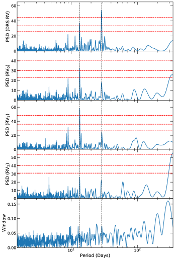
Figure 3: Lomb-Scargle periodograms of the DRS-reduced RVs, as well as the $RV_{0}$, $RV_{1}$, and $RV_{2}$ time series generated from our line lists. The 10%, 1%, and 0.1% False Alarm Probabilities (red dotted lines) are shown for each periodogram. The greatest power is concentrated in the solar synodic rotation period and its first harmonic (dotted gray lines), with no corresponding peaks in the window function (bottom panel).

3 Analysis

3.1 Solving for $\alpha$

If $\alpha$ is known, we can use experimentally determined values for $\rm RV_{0}$ and $\rm RV_{1}$ to extract theoretical time series of interest $\rm RV_{\rm conv}$ and $\rm RV_{\rm sppl}$. This process should isolate contributions from the suppression of convective blueshift, and leave behind common-mode planetary and photometric contributions in the corrected RV time series. In practice, however, we must estimate the parameter $\alpha$ by imposing assumptions on the reconstructed time series. We adopt methods to solve for the parameter $\alpha$ based on assumptions made for the reconstructed time series from M17. These methods rely predominantly on the assumption that $\rm RV_{\rm conv}$ dominates the RV time series. We applied the five methods detailed in M17 to solve numerically for the value of $\alpha$ that: 1) minimizes the mean absolute value of $\rm RV_{\rm sppl}$; 2) minimizes the correlation between $\rm RV_{\rm conv}$ and $\rm RV_{\rm sppl}$; 3) is the slope of $\rm RV_{1}$ vs $\rm RV_{0}$; 4) maximizes the ratio of the variance in $\rm RV_{\rm conv}$ vs that in $\rm RV_{\rm sppl}$; 5) maximizes that ratio when $\rm RV_{\rm sppl}$ is smoothed over 30 days, to average over rotationally modulated activity-induced variations. Additionally, 6) we calculate a best estimate for $\alpha$ as the ratio of the mean values of absolute RV time series derived from $\langle\rm RV_{\rm 1}\rangle/\langle\rm RV_{\rm 0}\rangle$ or $\langle\rm RV_{\rm 2}\rangle/\langle\rm RV_{\rm 0}\rangle$.

Table 4: Estimates for $\alpha$, and RMS variation for extracted $\rm RV_{\rm sppl}$ time series (m s^-1) from different methods. Method 2 fails to converge likely due to correlated noise, as discussed in M17

Method	$\rm RV_{1},\alpha$	$\rm RV_{1},std(\rm RV_{\rm sppl})$	$\rm RV_{2},\alpha$	$\rm RV_{2},std(\rm RV_{\rm sppl})$
1) $\langle\rm RV_{\rm sppl}\rangle=0$	.79	3.54	1.26	3.60
2) Minimize correlation between $\rm RV_{\rm sppl},\rm RV_{\rm conv}$	N/A	N/A	N/A	N/A
3) Slope of $\rm RV_{i}$ vs $\rm RV_{0}$	.97	22.63	1.03	28.54
4) Maximize $\rm std(\rm RV_{\rm conv})/\rm std(\rm RV_{\rm sppl})$	.99	67.79	1.01	85.56
5) Maximize $\rm std(\rm RV_{\rm conv})/std(\rm RV_{\rm sppl}\rm\;smoothed\ 30\ days)$	.73	2.91	1.34	2.91
6) $\langle\rm RV_{\rm i,abs}\rangle/\langle\rm RV_{\rm 0,abs}\rangle$	.74	2.99	1.32	3.05

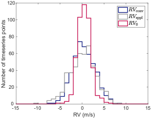
Figure 4: Histogram of timeseries points of $\rm RV_{0}$, and treated timeseries $\rm RV_{\rm sppl}$, $\rm RV_{\rm sppl}$ reconstructed using $\rm RV_{1}$ for $\alpha=.73$: this reconstruction had the lowest RV RMS for $\rm RV_{\rm sppl}$. As shown, this reconstruction fails to reduce the RMS from the initial timeseries $\rm RV_{0}$.

These values are shown in Table 4. Despite the relatively consistent observational sampling and high SNR of over 300 per exposure with an average of over 50 exposures per day, values for $\alpha$ differ based on the choice of assumption. Crucially, no physically motivated choice of $\alpha$ reduces the variability of $\rm RV_{\rm sppl}$, the corrected RV time series, compared to $\rm RV_{0}$, the untreated time series, as illustrated in Figure 4.

4 Discussion

Despite the higher SNR and better observational sampling for solar spectra, we are unable to extract physically significant reconstructed time series $\rm RV_{\rm conv}$ and $\rm RV_{\rm sppl}$ using the model and methods described in M17, suggesting that one of the assumptions of the model is not satisfied on this dataset. Crucially, the methods to estimate $\alpha$ assume that $\rm RV_{\rm conv}$ strongly dominates the RV timeseries. Potentially important is that our data set spans the activity minimum of the solar cycle, unlike the synthetic dataset from M17, which included a full solar activity cycle: the assumption that $\rm RV_{\rm conv}$ strongly dominates the RV time series might not hold for these restricted observations. Since the process of inverting the linear equations that describe $\left(\rm RV_{0},\rm RV_{1}\right)$ to extract $\left(\rm RV_{\rm sppl},\rm RV_{\rm conv}\right)$ amplifies all non-$\rm RV_{\rm conv}$ contributions, weakened $\rm RV_{\rm conv}$ at solar minimum could explain the inability to extract physical values of $\alpha$ on this data set. Our inability to reduce RV variability by applying the methods of M17 implies that sources of RV variability other than $\rm RV_{\rm conv}$ must be taken into account.

Additional results in the literature have shown that other processes besides $\rm RV_{\rm conv}$ may indeed play a dominant role near the solar minimum. For example, recent techniques demonstrate the ability to remove most power at the rotation period, but leave 1 m s^-1 RV variability in corrected timeseries: Dumusque (2018) and Cretingier et al. (2019, in revision) identify spectral lines insensitive to the suppression of convective blueshift; by computing RVs using these specially-selected line lists, the authors are able to reduce the RV RMS by a factor of 2.2, down to 0.9 m s^-1. Independently, Milbourne et al. (2019) use solar images from HMI/SDO to reproduce the activity-driven RVs. This analysis successfully removes the activity-driven signal at the rotation period, but still leaves an RMS amplitude of 1.2 m s^-1. Using independent analysis frameworks, both techniques successfully remove the rotationally-modulated activity signal, but are still limited by some other processes. Other work is ongoing to characterize the contributions from granulation and supergranulation, which can contribute as much as 1 m s^-1 to RV RMS (Dumusque et al., 2011; Meunier et al., 2015; Meunier & Lagrange, 2019; Cegla et al., 2019). The fact that our RV timeseries contain power concentrated at the rotation period and its harmonics is consistent with some significant $\rm RV_{\rm conv}$ contribution. The inability to significantly reduce RV RMS using the methods of M17 makes sense in the context of Milbourne et al. (2019), Dumusque (2018), the literature on granulation and supergranulation, which demonstrate that well over 1 m/s of RV variation remains after accounting for $\rm RV_{\rm conv}$.

When the linear equations defining $\rm RV_{0}$ and $\rm RV_{1}$ in terms of $\rm RV_{\rm sppl}$ and $\rm RV_{\rm conv}$ are inverted in the presence of noise introduced by this external variability, the RMS of noise in $\rm RV_{\rm sppl}$ is magnified to twice as large as the original RMS of noise in $\rm RV_{0}$ (M17). Potential contributions from instrumental systematics due to wavelength calibration (Cosentino et al., 2014; Dumusque, 2018; Cersullo et al., 2019; Coffinet et al., 2019), or daily calibration sequences (Collier Cameron et al., 2019), may also contribute significantly to this non-$\rm RV_{\rm conv}$ RV variability. This sensitivity to RV contributions other than $\rm RV_{\rm conv}$ motivates future consideration of different solar activity processes, especially those operating on different timescales such as magnetoconvection (Palle et al., 1995; Del Moro, 2004; Meunier, 2018). Furthermore, these additional processes, and even the suppression of convective blueshift itself, may contain subtle line list dependency, based on proxies for line responsiveness to magnetic activity such as the Lande-g factor (e.g., Norton et al. 2006). All of these contributions must be accounted for in order to reach the 10 cm s^-1 detection limit of an Earth-like planet orbiting a Sun-like star. Future work is needed to identify correlates in spectra, solar images, or some other ancillary dataset that could be used to model these phenomenon.

References

- Baranne et al. (1996) Baranne, A., Queloz, D., Mayor, M., et al. 1996, A&AS, 119, 373
- Berdyugina & Järvinen (2005) Berdyugina, S. V., & Järvinen, S. P. 2005, Astronomische Nachrichten, 326, 283
- Bergemann et al. (2019) Bergemann, M., Gallagher, A. J., Eitner, P., et al. 2019, A&A, 631, A80
- Borucki et al. (2010) Borucki, W. J., Koch, D., Basri, G., et al. 2010, Science, 327, 977
- Cegla et al. (2013) Cegla, H. M., Shelyag, S., Watson, C. A., & Mathioudakis, M. 2013, ApJ, 763, 95
- Cegla et al. (2019) Cegla, H. M., Watson, C. A., Shelyag, S., Mathioudakis, M., & Moutari, S. 2019, ApJ, 879, 55
- Cersullo et al. (2019) Cersullo, F., Coffinet, A., Chazelas, B., Lovis, C., & Pepe, F. 2019, A&A, 624, A122
- Coffinet et al. (2019) Coffinet, A., Lovis, C., Dumusque, X., & Pepe, F. 2019, A&A, 629, A27
- Collier Cameron et al. (2019) Collier Cameron, A., Mortier, A., Phillips, D., et al. 2019, MNRAS, 487, 1082
- Cosentino et al. (2012) Cosentino, R., Lovis, C., Pepe, F., et al. 2012, Proc.SPIE, 8446, 657
- Cosentino et al. (2014) —. 2014, Proc.SPIE, 9147, 2658
- Cretingier et al. (2019, in revision) Cretingier, M., Dumusque, X., Allart, R., Pepe, F., & Lovis, C. 2019, in revision, A&A
- Del Moro (2004) Del Moro, D. 2004, A&A, 428, 1007
- Dravins et al. (1981) Dravins, D., Lindegren, L., & Nordlund, A. 1981, A&A, 96, 345
- Dumusque (2018) Dumusque, X. 2018, A&A, 620, A47
- Dumusque et al. (2014) Dumusque, X., Boisse, I., & Santos, N. C. 2014, ApJ, 796, 132
- Dumusque et al. (2011) Dumusque, X., Udry, S., Lovis, C., Santos, N. C., & Monteiro, M. J. P. F. G. 2011, A&A, 525, A140
- Dumusque et al. (2015) Dumusque, X., Glenday, A., Phillips, D. F., et al. 2015, ApJL, 814, L21
- Fischer et al. (2016) Fischer, D. A., Anglada-Escude, G., Arriagada, P., et al. 2016, PASP, 128, 066001
- Giorgini et al. (1996) Giorgini, J. D., Yeomans, D. K., Chamberlin, A. B., et al. 1996, in Bulletin of the American Astronomical Society, Vol. 28, AAS/Division for Planetary Sciences Meeting Abstracts #28, 1158
- Gray (2005) Gray, D. 2005, The Observation and Analysis of Stellar Photospheres (Cambridge University Press)
- Gray (2009) Gray, D. F. 2009, ApJ, 697, 1032
- Gray & Oostra (2018) Gray, D. F., & Oostra, B. 2018, ApJ, 852, 42
- Haywood et al. (2016) Haywood, R. D., Collier Cameron, A., Unruh, Y. C., et al. 2016, MNRAS, 457, 3637
- Howell et al. (2014) Howell, S. B., Sobeck, C., Haas, M., et al. 2014, PASP, 126, 398
- Isaacson & Fischer (2010) Isaacson, H., & Fischer, D. 2010, ApJ, 725, 875
- Kurucz (2005) Kurucz, R. L. 2005, http://kurucz.harvard.edu/sun/fluxatlas2005/
- Kurucz et al. (1984) Kurucz, R. L., Furenlid, I., Brault, J., & Testerman, L. 1984, Solar flux atlas from 296 to 1300 nm (National Solar Observatory)
- Mayor & Queloz (1995) Mayor, M., & Queloz, D. 1995, Nature, 378, 335
- Meunier (2018) Meunier, N. 2018, A&A, 615, A87
- Meunier et al. (2010a) Meunier, N., Desort, M., & Lagrange, A.-M. 2010a, A&A, 512, A39
- Meunier & Lagrange (2019) Meunier, N., & Lagrange, A.-M. 2019, A&A, 625, L6
- Meunier et al. (2015) Meunier, N., Lagrange, A.-M., Borgniet, S., & Rieutord, M. 2015, A&A, 583, A118
- Meunier et al. (2010b) Meunier, N., Lagrange, A.-M., & Desort, M. 2010b, A&A, 519, A66
- Meunier et al. (2017a) Meunier, N., Lagrange, A.-M., & Borgniet, S. 2017a, A&A, 607, A6
- Meunier et al. (2017b) Meunier, N., Lagrange, A.-M., Mbemba Kabuiku, L., et al. 2017b, A&A, 597, A52
- Milbourne et al. (2019) Milbourne, T. W., Haywood, R. D., Phillips, D. F., et al. 2019, ApJ, 874, 107
- Motalebi et al. (2015) Motalebi, F., Udry, S., Gillon, M., et al. 2015, A&A, 584, A72
- Nordlund et al. (2009) Nordlund, Å., Stein, R. F., & Asplund, M. 2009, Living Reviews in Solar Physics, 6, 2
- Norton et al. (2006) Norton, A. A., Graham, J. P., Ulrich, R. K., et al. 2006, Solar Physics, 239, 69
- Palle et al. (1995) Palle, P. L., Jimenez, A., Perez Hernandez, F., et al. 1995, ApJ, 441, 952
- Pepe et al. (2010) Pepe, F. A., Cristiani, S., Lopez, R. R., et al. 2010, Proc.SPIE, 7735, 209
- Phillips et al. (2016) Phillips, D. F., Glenday, A. G., Dumusque, X., et al. 2016, 9912, 2163
- Reiners et al. (2016) Reiners, A., Mrotzek, N., Lemke, U., Hinrichs, J., & Reinsch, K. 2016, A&A, 587, A65
- Ricker et al. (2014) Ricker, G. R., Winn, J. N., Vanderspek, R., et al. 2014, JJ. Astron. Telesc. Instrum. Syst., 1, 1
- Saar & Donahue (1997) Saar, S. H., & Donahue, R. A. 1997, ApJ, 485, 319
- Schrijver & Zwaan (2000) Schrijver, C. J., & Zwaan, C. 2000, Solar and Stellar Magnetic Activity, Cambridge Astrophysics (Cambridge University Press)
- Schroeter (1984) Schroeter, E. H. 1984, A&A, 139, 538
- Shelke & Verma (1985) Shelke, R. N., & Verma, V. K. 1985, Bulletin of the Astronomical Society of India, 13, 53
- Sosnowska et al. (2012) Sosnowska, D., Lodi, M., Gao, X., et al. 2012, Proc.SPIE, 8451, 661
- Stein (2012) Stein, R. F. 2012, Living Reviews in Solar Physics, 9, 4
- VanderPlas et al. (2012) VanderPlas, J., Connolly, A. J., Ivezić, Ž., & Gray, A. 2012, in 2012 Conference on Intelligent Data Understanding, 47
- VanderPlas & Ivezić (2015) VanderPlas, J. T., & Ivezić, Ž. 2015, ApJ, 812, 18
- Zechmeister & Kürster (2009) Zechmeister, M., & Kürster, M. 2009, A&A, 496, 577