An Analysis of the Shapes of Interstellar Extinction Curves. VII.
Milky Way Spectrophotometric Optical-through-Ultraviolet Extinction and Its $R$-Dependence

Abstract

We produce a set of 72 NIR through UV extinction curves by combining new HST/STIS optical spectrophotometry with existing IUE spectrophotometry (yielding gapless coverage from 1150 – 10000 Å) and NIR photometry. These curves are used to determine a new, internally consistent, NIR through UV Milky Way Mean Curve and to characterize how the shapes of the extinction curves depend on $R(V)$. We emphasize that while this dependence captures much of the curve variability, there remains considerable variation which is independent of $R(V)$. We use the optical spectrophotometry to verify the presence of structure at intermediate wavelength scales in the curves. The fact that the optical through UV portions of the curves are sampled at relatively high resolution makes them very useful for determining how extinction affects different broad band systems, and we provide several examples. Finally, we compare our results to previous investigations.

1 Introduction

Dust grains play a large number of roles in the interstellar medium (ISM), serving, for example, as the primary formation site for H₂, as an important heat source (via the photoelectric effect), and as a chemical reservoir for the heavy elements. Arguably, however, their most significant effect is in modulating the flow of electromagnetic radiation through interstellar space via the combined effect of absorption and scattering. The ability of grains to transmit, redirect, and transmute electromagnetic energy is enormously important to the physics of interstellar space and, perhaps most far-reaching, places profound limits on our ability to study the universe at optical and ultraviolet (UV) wavelengths.

Studies of the interstellar “extinction curve,” i.e., the wavelength dependence of the combined effect of absorption and scattering out of the line of sight, have shown it to be highly spatially variable. This poses significant problems since a detailed knowledge of the curve is essential in numerous astrophysical applications, such as reconstructing the intrinsic spectral energy distributions (SEDs) of objects ranging from nearby stars to the most distant galaxies or for understanding the deposition of electromagnetic energy in star forming regions. On the other hand, these variations are a boon for the study of the dust itself, since they reflect general differences in the grain populations from sightline to sightline. Understanding how the various spectral regions of the curves relate to each other and how they respond to changes in the interstellar environments can provide information critical for characterizing the size, composition, and structure of interstellar grains (e.g., Weingartner & Draine, 2001; Clayton et al., 2003; Zubko et al., 2004).

Detailed investigations of the wavelength dependence of interstellar extinction began with measurements in the optical, generally based on broadband photometry. Early on, it was discovered that optical extinction curves may vary in shape from sightline to sightline, as exemplified by the 2.2 $\mu m^{-1}$ “knee” reported by Whitford (1958). Higher resolution studied revealed the presence of the “Very Broad Structure,” first reported by Whiteoak (1966) and studied in detail by York (1971). This structure is apparent in the “continuum subtracted” residuals presented most recently by Maíz Apellániz et al. (2014). Equally early, it was recognized that some of these shape variations were related to the ratio of total-to-selective extinction, ${R(V)\equiv A(V)/E(B-V)}$ (Johnson & Borgman, 1963). The $R(V)$-dependence of optical and, also, UV extinction was later quantified by Cardelli et al. (1989), and it has become standard practice to represent extinction curves as a family whose broad characteristics are dependent on $R(V)$ (Fitzpatrick, 1999, 2004; Valencic et al., 2004; Gordon et al., 2009; Maíz Apellániz et al., 2014).

It is somewhat remarkable that – despite its observational accessibility – the optical is not the best-characterized region of the interstellar extinction curve. The difficulty in obtaining ground-based spectrophotometry and the resultant paucity of spectroscopic resolution studies of optical extinction have prevented detailed investigations of the optical extinction features, their spatial variability, and their relationship to features at other wavelengths. Remarkably, is it the UV, accessible only by space-based instruments, where extinction has been most extensively studied at spectroscopic resolution (Witt et al., 1984; Fitzpatrick & Massa, 1986, 1990, 1988; Aiello et al., 1988; Cardelli et al., 1989; Valencic et al., 2004; Gordon et al., 2009), primarily as a result of the large database of UV spectrophotometry obtained by the International Ultraviolet Explorer satellite (IUE).

To fill in this gap in our knowledge of optical extinction, and to better characterize the relationship between extinction in the optical and that at other wavelengths, we initiated a Hubble Space Telescope (HST) SNAP program using the low-resolution STIS optical and near-infrared (NIR) gratings to observe a carefully selected set of moderately-reddened early-type stars that were previously observed in the UV. These observations provide low-resolution spectrophotometry covering the spectral range from the NIR to the near-UV region, i.e., between $\sim$1 $\mu$m and $\sim$3000 Å. When coupled with the existing UV data, these yield well-calibrated, low resolution SEDs for the program stars from 1150 – 10000 Å  which can be used to construct detailed extinction curves. These data resolve most, if not all, structure in the curves shortward of 1 $\mu$m; characterize the detailed shapes of the extinction curves in largely unexplored spectral regions; reveal the degree of variability in NIR through near-UV curves; and allow us to relate this variability to that seen in the UV and infrared.

The current paper utilizes IUE and STIS low resolution spectrophotometry along with broadband NIR photometry from the Two Micron All-Sky Survey (2MASS) to study the $R(V)$-dependence of extinction along lines of sight sampling a range of Milky Way environments. A detailed analysis and characterization of the structure observed in optical extinction curves is addressed in a companion paper (Massa et al., 2020).

Section 2 describes the selection of sightlines used in our analysis, as well as the processing of the STIS, IUE, and 2MASS data. Section 3 explains how the extinction curves were derived. Section 4 presents our results along with an $R(V)=3.1$ curve (which is typical of the diffuse Milky Way environment) and an $R(V)$ parameterization which captures much of the sight line to sight line variation. Section 5 discusses our results and compares them to previous work. Finally, Section 6 summarizes our findings.

2 Observations and Data Processing

2.1 The Sample

Our selection of program stars is based on the HST SNAP Program 13760. The initial sample included 130 reddened, normal, Milky Way, near main sequence (luminosity class III – V) O7 – B9.5 stars. The techniques we use to determine extinction curves give excellent results for stars in this range (see §3.2). This sample was restricted to stars with existing UV spectrophotometry from IUE and NIR broadband photometry from the 2MASS project and comprised two overlapping sub-groups: 1) stars with moderate to high extinction ($E(B\!-\!V)$ $\gtrsim 0.20$ mag) which sample sight lines with extreme values of $R(V)$ or interesting Milky Way environments, and 2) stars which sample dust within Milky Way open clusters and star-forming regions that have the potential to sample small scale structure in the dust distribution. Examples of the first group can be found in Valencic et al. (2004) and Fitzpatrick & Massa (2007, hereafter F07), who summarize most of the previous IUE work, including the Clayton et al. (2000) data on low density sight lines. The second group includes stars in open clusters observed by Aiello et al. (1982); Panek (1983); Clayton & Fitzpatrick (1987); Boggs & Bohm-Vitense (1989); Fitzpatrick & Massa (1990); Hackwell et al. (1991).

Of the 130 Milky Way targets submitted for our SNAP program, 77 were observed. Four stars (HD 73882, HD 99872, HD 281159 and Cl* NGC 457 Pes 10) were eliminated from the sample because their STIS spectra show evidence for offset and overlapping spectra from one or more other stars lying in the dispersion direction. A fifth star, HD 164865, turned out to be a late B supergiant, B9 Iab, and could not be well fit by the models we use to produce our extinction curves. That left the final sample of 72 stars used in this paper. These stars are listed in Table 1 along with some of their basic properties (i.e., spectral type, V magnitude, $E(B\!-\!V)$, distance, and galactic coordinates). Membership in a stellar cluster is indicated by the cluster name in parenthesis in the first column of the table.

Figure 1 shows an example of a typical program star SED, for the case of HD 27778 (B3 V). Prominent stellar and interstellar features are indicated beneath the SED. The sources of the data are indicated near the top of the figure. All data used in this study were obtained from the IUE satellite (UV spectrophotometry), the HST (“G430L” and “G750L” optical spectrophotometry), and the 2MASS project (NIR JHK photometry). In the subsections below, we describe the acquisition, processing, and calibration of the three datasets.

Table 1: Basic Data for Program Stars

Star	Spectral	V	$E(B-V)$	Distance	$l$	$b$	Reference
	Type	(mag)	(mag)	(pc)	($\arcdeg$)	($\arcdeg$)
BD+44 1080	B6 III	9.12	0.85	521	$162.484$	$1.51$	1
BD+56 517 (NGC 869)	B1.5 V	10.50	0.56	2079	$134.612$	$-3.71$	2
BD+56 518 (NGC 869)	B1.5 V	10.60	0.59	2079	$134.612$	$-3.71$	3
BD+56 576 (NGC 884)	B2 III	9.38	0.54	2345	$135.047$	$-3.59$	4
BD+69 1231	B9.5 V	9.27	0.23	389	$110.255$	$11.36$	5
BD+71 92 (Cr 463)	$\cdots$	10.35	0.29	702	$126.824$	$9.48$	$\cdots$
CPD-41 7715 (NGC 6231)	B2 IV-Vn	10.53	0.44	1243	$343.413$	$1.18$	6
CPD-57 3507 (NGC 3293)	B1 V	9.27	0.20	2910	$285.832$	$0.08$	7
CPD-57 3523 (NGC 3293)	B1 II	8.02	0.27	2910	$285.867$	$0.07$	7
CPD-59 2591 (Tr 16)	$\cdots$	10.93	0.77	3200	$287.591$	$-0.74$	$\cdots$
CPD-59 2600 (Tr 16)	O6 V((f))	8.61	0.51	3200	$287.591$	$-0.74$	8
CPD-59 2625 (Tr 16)	B2 V	11.58	0.44	3200	$287.637$	$-0.68$	9
GSC03712-01870	O5+	13.02	1.03	8200	$137.859$	$-0.97$	10
HD 13338	B1 V	9.06	0.51	1506	$133.513$	$-3.27$	11
HD 14250 (NGC 884)	B1 III	8.97	0.58	2345	$134.802$	$-3.72$	3
HD 14321 (NGC 884)	B1 IV	9.22	0.53	2345	$134.938$	$-3.85$	2
HD 17443	B9 V	8.74	0.38	284	$133.924$	$7.55$	12
HD 18352	B1 V	6.83	0.47	566	$137.715$	$2.16$	11
HD 27778	B3 V	6.36	0.36	262	$172.759$	$-17.38$	13
HD 28475	B5 V	6.79	0.27	254	$185.139$	$-25.09$	14
HD 29647	B8 III	8.31	1.00	157	$174.042$	$-13.35$	15
HD 30122	B5 III	6.34	0.26	371	$176.616$	$-14.03$	13
HD 30675	B3 V	7.53	0.52	355	$173.597$	$-10.20$	16
HD 37061 (NGC 1978)	B0.5 V	6.83	0.53	2429	$208.927$	$-19.28$	17
HD 38087	B5 V	8.30	0.30	315	$207.073$	$-16.26$	17
HD 40893	B0 IV:	8.90	0.44	2632	$180.091$	$4.33$	11
HD 46106 (NGC 2244)	B1 V	7.92	0.41	1670	$206.188$	$-2.10$	18
HD 46660 (NGC 2264)	B1 V	8.04	0.59	667	$201.173$	$1.46$	11
HD 54439	B2 IIIn	7.69	0.29	1295	$225.402$	$-1.69$	11
HD 62542	B5 V	8.07	0.31	396	$255.923$	$-9.25$	19
HD 68633	B5 V	8.00	0.48	274	$266.224$	$-9.55$	20
HD 70614	B6	9.27	0.67	$\cdots$	$259.807$	$-3.24$	20
HD 91983 (NGC 3293)	B1 III	8.58	0.28	2910	$285.882$	$0.05$	21
HD 92044 (NGC 3293)	B0.5 II	8.25	0.40	2910	$285.937$	$0.06$	21
HD 93028 (Cr 228)	O9 V	8.37	0.21	2201	$287.643$	$-1.20$	8
HD 93222 (Cr 228)	O7 III((f))	8.10	0.35	2201	$287.726$	$-1.01$	8
HD 104705	B0.5 III	7.79	0.27	2082	$297.465$	$-0.34$	11
HD 110336	B9 IV	8.64	0.45	333	$302.463$	$-14.50$	22
HD 110946	B1 V:	9.14	0.50	1509	$302.417$	$-2.06$	23
HD 112607	B7/B8 III	8.06	0.31	531	$303.784$	$-0.78$	22
HD 142096	B2.5 V	5.03	0.15	94	$350.724$	$25.38$	24
HD 142165	B6 IVn	5.37	0.11	128	$347.514$	$22.15$	24
HD 146285	B8 V	7.93	0.32	208	$351.012$	$18.20$	24
HD 147196	B5 V	7.04	0.26	272	$352.811$	$18.25$	25
HD 147889	B2 V	7.90	1.09	153	$352.868$	$17.04$	26
HD 149452	O8 Vn((f))	9.06	0.87	1636	$337.455$	$0.04$	8
HD 164073	B3 III/IV	8.03	0.20	961	$344.171$	$-12.56$	20
HD 172140	B0.5 III	9.95	0.21	7318	$5.274$	$-10.61$	27
HD 193322	O9 V:((n))	5.83	0.38	727	$78.110$	$2.78$	8
HD 197512	B1 V	8.56	0.32	1614	$87.895$	$4.63$	16
HD 197702	B1 III(n)	7.89	0.46	701	$73.925$	$-6.83$	28
HD 198781	B0.5 V	6.45	0.32	768	$99.956$	$12.62$	11
HD 199216	B1 II	7.03	0.74	1097	$88.922$	$3.04$	29
HD 204827 (Tr 37)	B0 V	7.94	1.11	835	$99.168$	$5.56$	30
HD 210072	B2 V	7.66	0.49	659	$100.844$	$-0.37$	26
HD 210121	$\cdots$	7.67	0.33	$\cdots$	$56.861$	$-44.47$	$\cdots$
HD 217086 (Cep OB3)	O7 Vn	7.64	0.92	724	$110.215$	$2.73$	8
HD 220057	B2 IV	6.93	0.23	770	$112.116$	$0.20$	31
HD 228969 (Br 86)	B2 II:	9.49	0.99	2429	$76.615$	$1.29$	11
HD 236960	B0.5 III	9.75	0.72	3474	$134.601$	$-1.51$	26
HD 239693 (Tr 37)	B3 V	9.51	0.44	835	$98.824$	$4.72$	32
HD 239722 (Tr 37)	B2 IV	9.55	0.92	835	$100.339$	$5.05$	32
HD 239745 (Tr 37)	B1 V	8.91	0.53	835	$99.432$	$2.99$	32
HD 282485	B9 V	9.88	0.47	412	$172.220$	$-10.29$	33
HD 292167	O9 III:	9.25	0.69	2681	$211.630$	$-1.17$	11
HD 294264 (NGC 1977)	B3 Vn	9.53	0.49	476	$208.492$	$-19.16$	34
HD 303068 (NGC 3293)	B1 V	9.78	0.25	2910	$285.688$	$0.07$	7
NGC 2244 11 (NGC 2244)	B2 V	9.73	0.44	1670	$206.422$	$-2.02$	35
NGC 2244 23 (NGC 2244)	B2.5 V	11.21	0.47	1670	$206.311$	$-2.08$	36
Trumpler 14 6 (Tr 14)	B1 V	11.23	0.49	3200	$287.419$	$-0.59$	37
Trumpler 14 27 (Tr 14)	$\cdots$	11.30	0.57	3200	$287.399$	$-0.60$	$\cdots$
VSS VIII-10	B8 V	10.07	0.73	235	$359.518$	$-18.29$	38

References. — (1) Bouigue (1959); (2) Schild (1965); (3) (Johnson & Morgan, 1955); (4) Slettebak (1968); (5) Racine (1968b); (6) Schild et al. (1971); (7) Turner et al. (1980); (8) Maíz-Apellániz et al. (2004); (9) Massey & Johnson (1993); (10) Muzzio & Rydgren (1974); (11) Morgan et al. (1955); (12) Racine (1968a); (13) Osawa (1959); (14) Cowley et al. (1969); (15) Metreveli (1968); (16) Guetter (1968); (17) Schild & Chaffee (1971); (18) Johnson & Morgan (1953); (19) Feast et al. (1955); (20) Houk (1978); (21) Hoffleit (1956); (22) Houk & Cowley (1975); (23) Feast et al. (1957); (24) Garrison (1967); (25) Borgman (1960); (26) Hiltner (1956); (27) Hill (1970); (28) Walborn (1971); (29) Divan (1954); (30) Morgan et al. (1953); (31) Boulon et al. (1958); (32) Garrison & Kormendy (1976); (33) Roman (1955); (34) Smith (1972); (35) Meadows (1961); (36) Johnson (1962); (37) Morrell et al. (1988); (38) Vrba & Rydgren (1984)

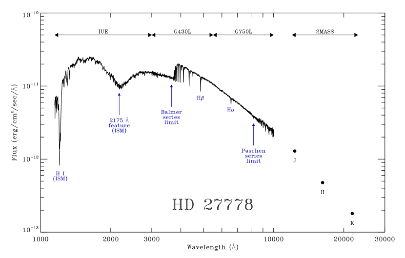
Figure 1: Representative spectral energy distribution (SED) for our program stars, using HD 27778 as an example. Sources and wavelength ranges of the various datasets are indicated at the top of the figure. International Ultraviolet Explorer satellite (IUE) data from the SWP, LWP, and LWR cameras, covering the range 1150-3000 Å was obtained from the Mikulski Archive for Space Telescopes. New Hubble Space Telescope spectrophotometric observations using the G430L and G750L gratings were acquired for this program, and cover the ranges 3000-5450 Å and 5450-10000 Å, respectively. NIR JHK photometry from the Two Micron All-Sky Survey (2MASS) was obtained from the 2MASS archive maintained by the Infrared Processing and Analysis Center. Prominent stellar and interstellar features are identified beneath the SED.

2.2 Optical Data - HST

The optical data were all obtained as part of the HST SNAP Program 13760 and consist of STIS spectrophotometry with the G430L ($2900\leq\lambda\leq 5700$ Å) and G750L ($5240\leq\lambda\leq 10270$ Å) first order gratings. The total wavelength coverage is 2900–10270 Å with a resolution $\lambda/\Delta\lambda$ ranging from 530 to 1040 (e.g., Bostroem & Proffitt, 2011). The G430L observations are essential for determining the stellar parameters and had a minimum signal-to-noise (S/N) goal of 20:1 per pixel. G750L observations are always more problematic because of the sensitivity drop in the instrument of $\sim$5.5$\times$ from a peak at 7100 Å to 10000 Å and because moderately reddened OB stars are much fainter at longer wavelengths. For example, HD 27778 in Figure 1, with $E(B\!-\!V)$ = 0.36, drops by a factor of $\sim$2.5$\times$ over the same wavelength interval. Consequently, our G750L exposure times were limited to avoid saturation at the shortest wavelengths (assuming a mean extinction curve shape) and also to keep the total on-target time under 30 minutes to increase the potential for execution of our SNAP observations. As a result of these considerations, the S/N of the G750L data vary considerably with wavelength and from star-to-star.

The G430L and G750L spectra are processed with the Instrument Definition Team (IDT) pipeline software written in IDL by D. J. Lindler in 1996–1997. This IDL data reduction is more flexible and offers the following advantages over the STScI pipeline results that are available from the Mikulski Archive for Space Telescopes (MAST): (1) better compensation for small shifts in pointing or instrumental flexure that may occur between the images of a cosmic ray split (CR-split) observation; (2) a larger extraction window height for the G750L data, to compensate for an increase in the spectral width in recent years; (3) elimination of “hot” pixels from the extracted spectrum; and (4) the use of tungsten lamp spectra to remove CCD fringing effects in the G750L spectra. The processing technique is discussed more thoroughly in Appendix A.

In addition to the above data extraction advantages, our post-processing includes the charge transfer efficiency (CTE) corrections of Goudfrooij et al. (2006), and an up-to-date correction for the changes in STIS sensitivity with time and temperature. The observations of the three primary flux standards G191B2B, GD153, and GD71, as corrected for CTE and the latest measures of sensitivity change with time, produce the current absolute flux calibration (CALSPEC; see Bohlin et al., 2014).

After completion of all the processing steps, the data were concatenated, with G430L used below 5450 Å and G750L used above 5450 Å.

2.3 Ultraviolet Data - IUE

With the exception of GSC03712-01870, the stars included in this paper have all been incorporated in previous UV extinction studies, notably by Fitzpatrick & Massa (2005a, hereafter F05) and F07, and have IUE spectrophotometric observations available from both the short-wavelength region (“SWP” camera; 1150–1980 Å) and long-wavelength region (“LWR” or “LWP” cameras; 1980–3200 Å). Only SWP observations exist for GSC03712-01870. The IUE data were obtained by us from the MAST archive and were processed as described earlier (e.g., see F07). The critical step in the processing of the archival data was the correction for deficiencies in the IUE NEWSIPS calibration, using the results of Massa & Fitzpatrick (2000, hereafter M00). These deficiencies include systematic thermal and temporal effects and an incorrect absolute calibration. This is particularly important for our current study because we derive extinction curves using model atmosphere calculations, rather than unreddened comparison stars, and errors in the calibration of the data would be reflected directly in the resultant curves. The M00 corrections place the IUE data on the absolute flux calibration system as it was in the year 2000. The calibration has been modified in the intervening years and, to take advantage of this, we additionally corrected the data to the current CALSPEC standard. We did this by comparing M00-corrected IUE spectra of the flux standards G191B2B, GD71 and GD153 with the current SEDs of those stars as found in the CALSPEC database. This comparison indicated that the flux levels of M00-corrected IUE spectra need to be reduced by an average of $\sim$0.9% in the short-wavelength region and $\sim$1.8% in the long-wavelength region (with a roughly linear wavelength dependence across the whole IUE UV). This final correction makes the calibration of the IUE data fully consistent and compatible with the calibration of the optical HST spectrophotometry described above and the NIR photometry described below. When the processing was completed, the UV spectra for each star were trimmed to the wavelength range 1150–3000 Å, with the short- and long-wavelength camera data joined at a wavelength of 1978 Å.

2.4 NIR Data - 2MASS

The third dataset consists of NIR JHK photometry from 2MASS. These data were obtained from the 2MASS All-Sky Point Source Catalog, accessed via the 2MASS website hosted by the Infrared Processing and Analysis Center (IPAC). JHK measurements are available for all program stars although, due to lack of uncertainty estimates, we excluded the J and H data for the star CPD–57 3523. The 2MASS data required no additional processing.

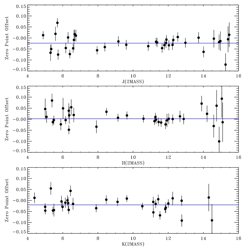
Figure 2: Calibration of synthetic 2MASS JHK photometry. Synthetic JHK magnitudes were computed for the model SEDs of 30-40 stars in the CALSPEC database, as described in §2.4, and “zero point offsets” determined to match the synthetic values to the observed 2MASS values. The top, middle, and bottom panels show these offsets for the $J$, $H$, and $K$ filters, respectively, plotted against the observed 2MASS magnitudes. Thick blue lines indicate the weighted mean offsets, with values of –0.023, 0.002, and –0.020 mag for $J$, $H$, and $K$, respectively. The error bars are those associated with the observed magnitudes.

The flux calibration of the 2MASS bands is important to our study because we derive NIR extinction by comparing the 2MASS magnitudes for reddened stars with synthetic values derived from the stars’ assumed intrinsic SEDs. Thus, the synthetic photometry must be calibrated in a manner consistent with the latest CALSPEC system. The standard 2MASS calibration was performed by Cohen et al. (2003), based on a synthetic spectrum of Vega (see Cohen et al., 1992) and the assumption that Vega defines zero magnitude in the 2MASS NIR. To assure consistency with our new study, we rederived this calibration, based on the latest CALSPEC database. We did this by computing synthetic 2MASS magnitudes for a subset of the CALSPEC calibration sample and then determining the transformation that maps these values to the observed 2MASS JHK magnitudes. The procedure is essentially identical to that used by Fitzpatrick & Massa (2005b) in a general calibration of synthetic photometry for B and early A-type stars. In this case, we began with the 40 flux standard stars from the CALSPEC Calibration Database for which NIR model fluxes were computed. This subset of the full calibration sample includes all the stars in Table 1 of the Database for which entries exist in Column (6), indicating the existence of a model SED, with the exception of SF1615+001A (no 2MASS data) and HZ43 (contamination of 2MASS by a red companion star). The sample was further restricted to those stars with 2MASS magnitude uncertainties less than 0.1 mag, leaving 37, 36, and 32 stars for calibration of the $J$, $H$, and $K$ filters, respectively. We performed synthetic photometry on the model SEDs (in $f_{\lambda}$ units) using the 2MASS JHK filter response functions and $F_{\lambda}$(0 mag) values from Cohen et al. (2003). The transformation to the observed 2MASS system is expressed in terms of “zero point offsets” as defined in Cohen et al. (2003) or, equivalently, in Equation 1 of Maíz Apellániz (2007). The results for each filter are shown in Figure 2, where we plot zero point offsets against the 2MASS magnitudes. The final adopted offsets are weighted means with values of –0.023, +0.002, and –0.020 mag for the $J$, $H$, and $K$ filters, respectively. These offsets are almost identical (i.e., within $\pm$0.005 mag) to those found by Maíz Apellániz & Pantaleoni González (2018), who also used the CALSPEC database to examine the 2MASS calibration. Like Maíz Apellániz & Pantaleoni González (2018), we find no evidence for color dependence in these offsets, nor for a systematic brightness dependence (as can be seen in Figure 2). Use of these zero point offsets assures that the 2MASS photometric data are calibrated consistently with our UV and optical spectrophotometric datasets.

3 Creating the NIR-UV Extinction Curves

We derive NIR through UV extinction curves for our 72 program stars using the “Extinction-Without-Standards” approach, first described by F05. This technique utilizes SEDs from stellar atmosphere models to represent the intrinsic SEDs of the reddened program stars, rather than observations of unreddened stars of similar spectral type. The advantages of such an approach are described in detail in F05. In our previous applications of Extinction-Without-Standards (e.g., F05 and F07), we determined the stellar properties and the extinction properties simultaneously by fitting IUE UV spectrophotometry and optical/near-IR photometry with model SEDs and a parameterized version of the interstellar extinction curve. In this study, we adopt a slightly different approach, explicitly separating the process into two distinct steps: (1) first, we determine the appropriate stellar properties needed to characterize the model SED, and then (2) form a normalized ratio between the observed and model SEDs (i.e., the extinction curve). This approach is made possible by the new HST spectrophotometry, which allows a detailed modeling of critical stellar diagnostics in the optical spectral region. The advantage is that the resultant extinction curves are derived completely empirically, without any assumptions as to their underlying functional form. The two steps in this process are described separately in the following subsections.

3.1 Step 1: Determining the Stellar Properties

We estimate the intrinsic properties of our program stars by fitting their G430L spectra with stellar atmosphere models. The HST’s G430L data consist of spectrophotometric observations over the wavelength range 2900–5700 Å at a resolution better than 10 Å. As such, they provide a clear view of the wide range of spectroscopic features present in the classical blue spectral region, which formed the basis of the spectral classification system. Thus, ample information is present in these data to determine stellar effective temperature ($T_{\rm eff}$), surface gravity ($\log g$) and, more coarsely, metallicity ([m/H]).

For most of our program stars, we fit the G430L data using the TLUSTY NLTE SED grids published by Lanz & Hubeny (2003, “OSTAR2002”) and Lanz & Hubeny (2007, “BSTAR2006”). The grids were computed at full spectral resolution (at the thermal broadening level) and, together, cover a wide range of metallicities ([m/H] = +0.3 to –1.0), effective temperatures ($T_{\rm eff}$ = 15,000 K to 55,000 K), and surface gravities ($\log g$ = 4.75 to the modified Eddington limit). The OSTAR2002 grid assumes a microturbulence velocity of $v_{turb}$ = 10 km s^-1, while the BSTAR2006 grid assumes $v_{turb}$ = 2 km s^-1, with a small number of low gravity models computed with $v_{turb}$ = 10 km s^-1. Both grids assume the solar abundance scale of Grevesse & Sauval (1998). The modeling process involves four steps: (1) begin with initial estimates of $T_{\rm eff}$, $\log g$, and [m/H]; (2) interpolate within the appropriate TLUSTY grid to produce a full-resolution SED, F_λ, with these properties in the G430L spectral range; (3) broaden the SED to account for the effects of stellar rotation and the instrumental profile of the G430L and (4) compare the model SED with the G430L spectrum, using $\chi^{2}$ as the measure of the goodness-of-fit. The initial estimates of the stellar properties were then adjusted and the process repeated iteratively until the minimum value of $\chi^{2}$ was achieved. The broadband shapes and levels of the G430L SEDs are distorted relative to the models due to the effects of distance and interstellar extinction. To remove these effects from the analysis, we mapped the overall shapes of the model continua onto the observed continua using a cubic spline, whose anchor points were iteratively adjusted along with the stellar properties. Thus, the final stellar properties determined from the fitting procedure depend only on the absorption line spectrum (plus the Balmer jump) and not at all on the general shape of the spectrum. The continuum mapping is not used in the subsequent derivation of the extinction curves.

The broadening applied to the model SEDs requires some additional discussion. In early tests, we applied a Gaussian PSF with FWHM = 5.5 Å, as taken from the STIS Instrument Handbook (Riley et al., 2019), and rotational broadening based on $v\sin i$ values from the literature. In a number of cases, however, the observed spectra appeared significantly more broadened, consistent (in the most extreme cases) with a PSF FWHM of 7.8 Å. The initially adopted value 5.5 Å appeared, in these tests, to be a minimum. We attribute these discrepancies to a variable PSF width in our slitless spectra, arising from focus changes due to thermal cycling of the instrument (aka “breathing”). Ideally, we would deal with this by adopting measured $v\sin i$ values for all the stars and allowing the FWHM of the PSF to be a free parameter in the fitting routine, adjusted to achieve a best-fit to the line profiles. Unfortunately, only about one-third of our program stars have measured $v\sin i$ values and so this is not feasible. Instead, we adopted a modified approach and fixed the PSF FWHM at the minimum observed value of 5.5 Å and varied the width of the rotational broadening profile to achieve a best-fit to the spectra. This yields a value of “$v_{broad}$”, which contains both the rotational broadening of the star and the effects of breathing. We found that, in cases where $v\sin i$ is known, these two different approaches yield essentially identical results, in both the values of $\chi^{2}$ and the model parameters. Evidently, the resolution and S/N of our data are such that the differences between a Gaussian and a rotational profile are not significant.

Eleven of the program stars have $T_{\rm eff}$ values below the 15,000 K lower limit of the TLUSTY BSTAR2006 grid. The general procedure for determining their properties is similar to that described above, except that in step (2) we used a combination of the ATLAS9 LTE models from Kurucz (1991) to produce an interpolated atmospheric structure for the desired stellar properties, and then the spectral synthesis program SPECTRUM (Version 2.76e) developed by Richard Gray (see Gray & Corbally, 1994) to produce a fully resolved stellar spectrum over the G430L spectral window. For consistency with the TLUSTY grids, these calculations also assumed the Grevesse & Sauval (1998) solar abundance scale.

Table 2: Stellar Properties from G430L Analysis

Star	$T_{eff}$	$\log g$	[m/H]	$v_{turb}$	$v_{broad}$	Atmosphere
	(K)			$\rm(km/s)$	$\rm(km/s)$	Model
BD+44 1080	$12879$	$3.42$	$-0.25$	$2$	$303$	ATLAS9/SPECTRUM
BD+56 517	$23752$	$3.76$	$-0.38$	$2$	$192$	TLUSTY B02
BD+56 518	$23415$	$3.80$	$-0.36$	$2$	$165$	TLUSTY B02
BD+56 576	$23275$	$3.48$	$-0.16$	$2$	$169$	TLUSTY B02
BD+69 1231	$11292$	$4.23$	$-0.16$	$2$	$413$	ATLAS9/SPECTRUM
BD+71 92	$11634$	$4.04$	$-0.21$	$2$	$325$	ATLAS9/SPECTRUM
CPD-41 7715	$23617$	$3.98$	$-0.23$	$2$	$322$	TLUSTY B02
CPD-57 3507	$25921$	$3.71$	$-0.19$	$2$	$192$	TLUSTY B02
CPD-57 3523	$25037$	$3.10$	$-0.34$	$10$	$255$	TLUSTY B10
CPD-59 2591	$34169$	$4.18$	$-0.25$	$10$	$332$	TLUSTY O10
CPD-59 2600	$38901$	$3.68$	$-0.22$	$10$	$338$	TLUSTY O10
CPD-59 2625	$26310$	$4.42$	$-1.03$	$2$	$137$	TLUSTY B02
GSC03712-01870	$33233$	$3.98$	$-0.50$	$10$	$229$	TLUSTY O10
HD 13338	$22748$	$3.61$	$-0.38$	$2$	$204$	TLUSTY B02
HD 14250	$24701$	$3.53$	$-0.16$	$2$	$350$	TLUSTY B02
HD 14321	$23294$	$3.57$	$-0.33$	$2$	$224$	TLUSTY B02
HD 17443	$11241$	$4.15$	$-0.16$	$2$	$397$	ATLAS9/SPECTRUM
HD 27778	$17362$	$3.91$	$-0.47$	$2$	$295$	TLUSTY B02
HD 28475	$15570$	$4.01$	$-0.44$	$2$	$368$	TLUSTY B02
HD 29647	$12356$	$3.58$	$-0.25$	$2$	$286$	ATLAS9/SPECTRUM
HD 30122	$16432$	$3.65$	$-1.05$	$2$	$341$	TLUSTY B02
HD 30675	$16428$	$3.97$	$-0.37$	$2$	$318$	TLUSTY B02
HD 37061	$28366$	$4.12$	$-0.51$	$10$	$332$	TLUSTY O10
HD 38087	$17408$	$4.20$	$-0.34$	$2$	$294$	TLUSTY B02
HD 40893	$31837$	$3.60$	$-0.19$	$10$	$335$	TLUSTY O10
HD 46106	$29265$	$4.10$	$-0.58$	$10$	$339$	TLUSTY O10
HD 46660	$31067$	$3.98$	$-0.53$	$10$	$303$	TLUSTY O10
HD 54439	$25300$	$3.71$	$-0.27$	$2$	$315$	TLUSTY B02
HD 62542	$17083$	$4.07$	$-0.55$	$2$	$302$	TLUSTY B02
HD 68633	$18643$	$3.91$	$-0.52$	$2$	$277$	TLUSTY B02
HD 70614	$18105$	$3.25$	$-0.39$	$2$	$333$	TLUSTY B02
HD 91983	$24490$	$3.36$	$-0.12$	$2$	$232$	TLUSTY B02
HD 92044	$24529$	$3.06$	$-0.28$	$10$	$247$	TLUSTY B10
HD 93028	$33564$	$4.04$	$-0.21$	$10$	$252$	TLUSTY O10
HD 93222	$36349$	$3.66$	$-0.24$	$10$	$296$	TLUSTY O10
HD 104705	$29222$	$3.44$	$-0.02$	$10$	$307$	TLUSTY O10
HD 110336	$11941$	$4.15$	$-0.17$	$2$	$300$	ATLAS9/SPECTRUM
HD 110946	$20582$	$3.24$	$-0.53$	$10$	$249$	TLUSTY B10
HD 112607	$12980$	$3.43$	$-0.22$	$2$	$347$	ATLAS9/SPECTRUM
HD 142096	$18205$	$4.34$	$-0.29$	$2$	$330$	TLUSTY B02
HD 142165	$14230$	$4.20$	$-0.31$	$2$	$398$	ATLAS9/SPECTRUM
HD 146285	$12328$	$4.36$	$-0.18$	$2$	$353$	ATLAS9/SPECTRUM
HD 147196	$12225$	$3.94$	$-0.45$	$2$	$544$	ATLAS9/SPECTRUM
HD 147889	$22061$	$4.13$	$-0.54$	$2$	$229$	TLUSTY B02
HD 149452	$31816$	$3.55$	$-0.00$	$10$	$405$	TLUSTY O10
HD 164073	$17573$	$3.99$	$-0.43$	$2$	$333$	TLUSTY B02
HD 172140	$27347$	$3.77$	$0.06$	$10$	$232$	TLUSTY O10
HD 193322	$33358$	$3.90$	$-0.19$	$10$	$387$	TLUSTY O10
HD 197512	$23773$	$3.83$	$-0.41$	$2$	$165$	TLUSTY B02
HD 197702	$23854$	$2.99$	$-0.38$	$10$	$430$	TLUSTY B10
HD 198781	$25529$	$3.13$	$-0.49$	$10$	$284$	TLUSTY B10
HD 199216	$24140$	$3.04$	$-0.34$	$10$	$189$	TLUSTY B10
HD 204827	$32037$	$3.96$	$-0.28$	$10$	$345$	TLUSTY O10
HD 210072	$19186$	$3.08$	$-0.55$	$10$	$312$	TLUSTY B10
HD 210121	$16498$	$4.06$	$-0.29$	$2$	$290$	TLUSTY B02
HD 217086	$35722$	$3.65$	$-0.34$	$10$	$443$	TLUSTY O10
HD 220057	$19736$	$4.21$	$-0.38$	$2$	$396$	TLUSTY B02
HD 228969	$28818$	$3.84$	$-0.28$	$10$	$378$	TLUSTY O10
HD 236960	$26572$	$3.47$	$0.11$	$2$	$229$	TLUSTY B02
HD 239693	$18885$	$4.11$	$-0.33$	$2$	$357$	TLUSTY B02
HD 239722	$20146$	$3.79$	$-0.62$	$2$	$210$	TLUSTY B02
HD 239745	$27059$	$4.12$	$-0.37$	$2$	$215$	TLUSTY B02
HD 282485	$12927$	$3.88$	$-0.26$	$2$	$309$	ATLAS9/SPECTRUM
HD 292167	$28817$	$3.01$	$-0.21$	$10$	$225$	TLUSTY O10
HD 294264	$19095$	$4.23$	$-0.37$	$2$	$300$	TLUSTY B02
HD 303068	$24810$	$3.80$	$-0.29$	$2$	$203$	TLUSTY B02
NGC 2244 11	$27166$	$4.13$	$-0.37$	$2$	$296$	TLUSTY B02
NGC 2244 23	$19091$	$4.06$	$-0.29$	$2$	$440$	TLUSTY B02
Trumpler 14 6	$28047$	$4.09$	$-0.22$	$2$	$243$	TLUSTY B02
Trumpler 14 27	$25998$	$4.17$	$-0.45$	$2$	$178$	TLUSTY B02
VSS VIII-10	$11525$	$3.76$	$-0.30$	$2$	$393$	ATLAS9/SPECTRUM

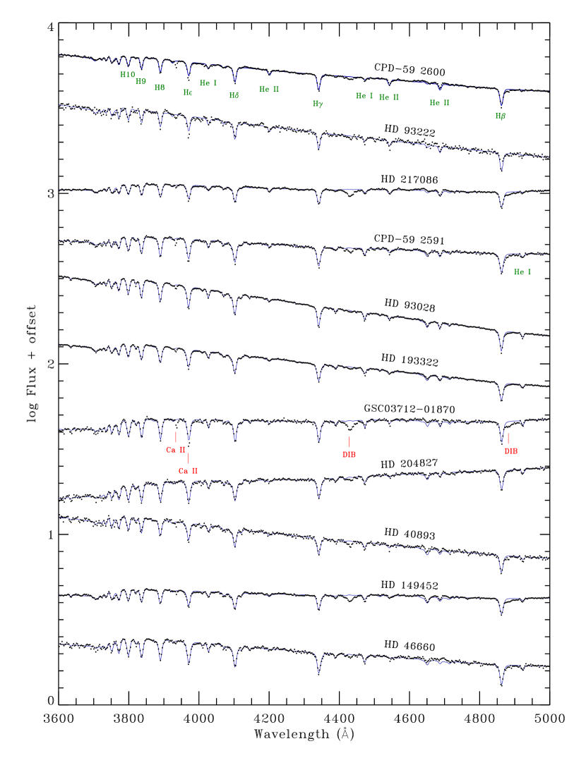
Figure 3a: Model atmosphere fits to the G430L spectra of the program stars. Small black circles show the observed G430L spectrum over the wavelength range 3600–5000 Å. Solid blue curves show the best-fitting stellar atmosphere models. The fitting procedure is described in §3.1 and included the full range of the G430L spectra (2900–5700 Å). Most of the spectral features are contained in the narrower range shown in the figure. Prominent stellar features are identified in green and interstellar features, including gas-phase absorption lines and diffuse interstellar bands (“DIB”), are identified in red. The stars are ordered in decreasing $T_{\rm eff}$, throughout the figures. Stellar properties derived from the fits are listed in Table 2.

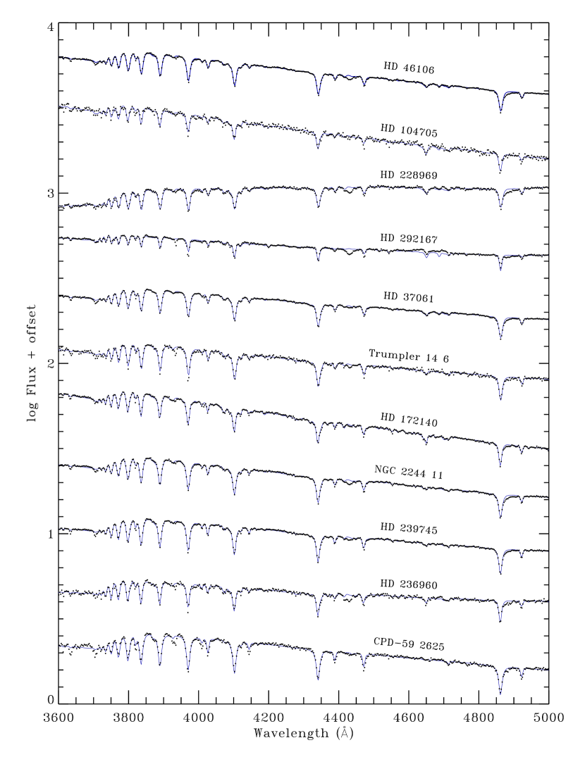
Figure 3b: Same as Figure 3a.

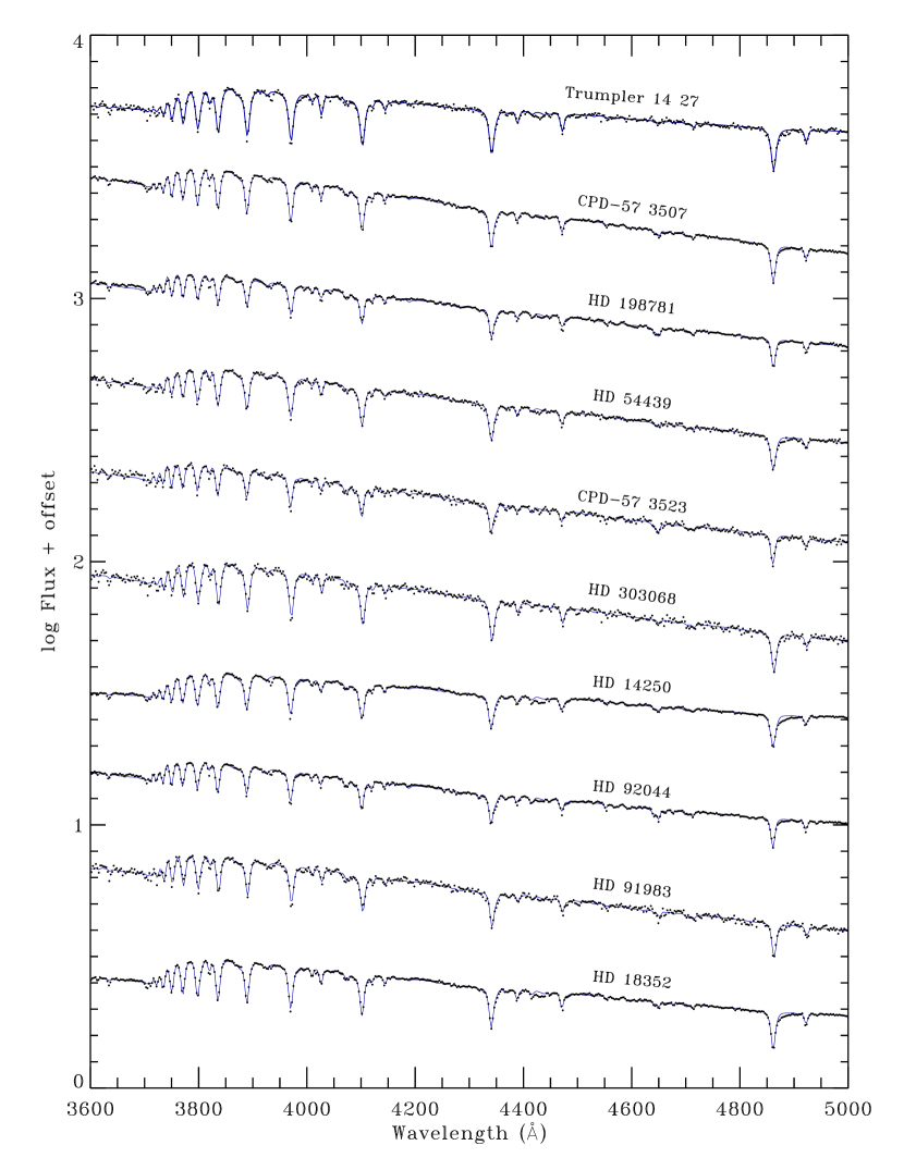
Figure 3c: Same as Figure 3a.

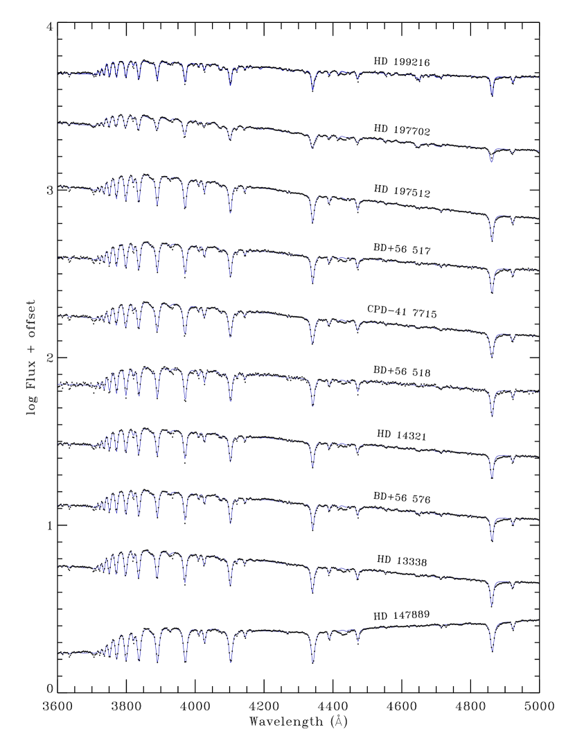
Figure 3d: Same as Figure 3a.

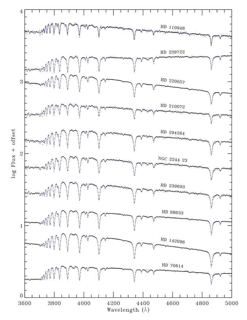
Figure 3e: Same as Figure 3a.

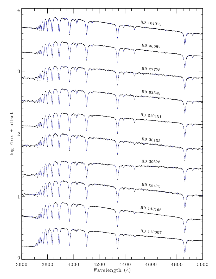
Figure 3f: Same as Figure 3a.

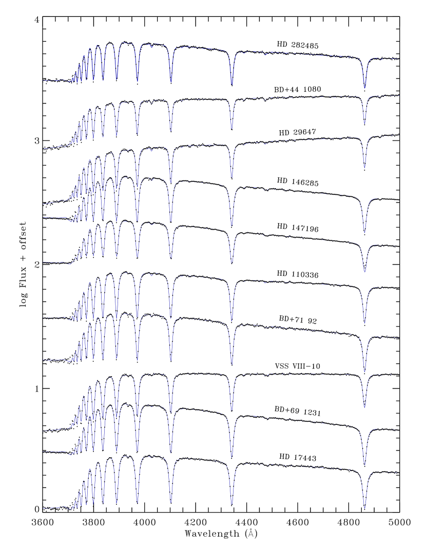
Figure 3g: Same as Figure 3a.

The ability of the stellar models to reproduce the G430L spectra is demonstrated in Figure 3. The various panels show the observed G430L data (small black filled circles) overlaid with the best fit models (solid blue lines). For clarity, the stars are ordered by decreasing $T_{\rm eff}$, from the top of Figure 3a (hottest star) to the bottom of Figure 3g (coolest star). Prominent stellar features are identified and labeled in green, while interstellar features are labeled in red. As seen in the figures, the models reproduce the observed stellar features very well. The only significant and systematic discrepancies noticeable in Figure 3 are due to interstellar features, notably the broad diffuse interstellar bands (“DIBs”) at 4430 Å and 4870 Å and the Ca II H and K absorption lines at 3968 Å and 3933 Å, respectively, which are identified in the first panel of Figure 3. Four stars in the sample (HD 147196, HD 197702, HD 292167, and VSS VII-10) show evidence for mild H$\alpha$ emission in their G750L spectra, which is not reproduced by the atmosphere models. Two of these stars (HD 197702 and HD 292167) are early-type giants at the low gravity edge of our adopted model grids ($\log g$ $\sim$3.0). The other two are late-B main sequence stars and may be rapid rotators. Indeed, HD 147196 has the largest value of $v_{broad}$ among our sample. In all four cases, however, the blue region of the spectra appear normal (as seen in Figure 3), as does the UV region, and we believe that the stellar parameters and SEDs are well reproduced by the models used here. (Note that the rapidly rotating HD 147196 will ultimately be excluded from the final extinction sample analyzed below due to its low value of $E(B\!-\!V)$.)

The final set of parameters describing the best-fit models are listed in Table 2. In addition to the values of $T_{\rm eff}$, $\log g$  [m/H], $v_{turb}$, and $v_{broad}$, we also indicate – in the last column of the table – the particular stellar atmosphere grid used for each star. In cases where the stellar properties fell into regions in which the different TLUSTY grids overlapped, we choose the model which yielded the best fit to the data.

The typical statistical uncertainties in the stellar parameters derived from the fitting procedure are $\pm$200 K in $T_{\rm eff}$, $\pm$0.02 in $\log g$, $\pm$0.1 in [m/H], and $\pm$10 km s^-1 in $v_{broad}$. These, however do not take into account systematic effects that could arise from the fundamental assumptions in the modeling process. For example, the solar abundances of Grevesse & Sauval (1998) have been superceded since the TLUSTY grids were computed (Grevesse et al., 2013). In addition, the overlap region between the cool TLUSTY BSTAR2006 models and the ATLAS9/SPECTRUM models is illustrative. For any star for which the BSTAR2006 models indicated $T_{\rm eff}$ $<$ 15,000 K, we adopted the ATLAS9/SPECTRUM combination described above. However, when experimenting with the ATLAS9/SPECTRUM combination for stars warmer the 15,000 K, we found that they yielded $T_{\rm eff}$ values several hundred K hotter than the best-fit TLUSTY models. This is undoubtedly due to the fundamental difference in the LTE vs. NLTE approaches and, possibly, to differences in the base opacities and atomic parameters assumed in the models. It would be useful to repeat this comparison with other LTE model grids, e.g., the BOSZ grid of Bohlin et al. (2017). However, while this is an interesting stellar atmospheres issue, fortunately for us it has little impact on the derived extinction curves. As was shown by Massa et al. (1983), the effects of temperature mismatch in extinction curves formed from early-type stars tend to be self-canceling due to the optical normalization (which, with some modifications, we will adopt here). Moreover, the wide range in intrinsic extinction curve properties also serves to lessen the impact of the relatively small uncertainties in the intrinsic stellar properties.

3.2 Step 2: Constructing the Extinction Curves

Once the properties of the reddened stars were determined, the production of the normalized extinction curves was straightforward. $A(\lambda)$, the total extinction at a wavelength $\lambda$, is given by:

$$A(\lambda)=-2.5\times\log\frac{f_{\lambda}}{\rm F_{\lambda}}+5\times\log\frac{R_{*}}{d}$$ (1)

where $f_{\lambda}$ and $\rm F_{\lambda}$ are the observed and intrinsic SEDs, respectively, and the quantity $R_{*}/d$ is the angular radius of the star, i.e., its physical radius $R_{*}$ divided by its distance $d$. Since these latter two quantities are rarely known accurately, extinction is usually presented in a normalized form, in which the angular radius cancels out. In this paper, we adopt the normalization:

$$k(\lambda-55)\equiv\frac{E(\lambda-55)}{E(44-55)}=\frac{A(\lambda)-A(55)}{A(44)-A(55)}$$ (2)

and:

$$R(55)\equiv\frac{A(55)}{E(44-55)}$$ (3)

These are analogous to the most commonly used normalizations of extinction, i.e., $k(\lambda-V)\equiv E(\lambda-V)/E(B-V)$ and $R(V)$, but with monochromatic measures of the extinction at 4400 Å and 5500 Å substituting for measurements with the Johnson $B$ and $V$ filters, respectively. The monochromatic values were determined by interpolation of a quadratic fit to the extinction curves over a range $\pm$0.1$\mu{\rm m}^{-1}$ from the desired wavelength. The benefit of the monochromatic normalization is that it eliminates bandpass effects in the extinction measurements. Such effects will be illustrated further in §4.3. Because the effective wavelengths of the broad Johnson filters depend on the shape of a stellar SED (and thus on $E(B\!-\!V)$ and $T_{\rm eff}$), there is no unique transformation between $k(\lambda\!-\!V)$ and $k(\lambda\!-\!55)$. For our whole sample, which consists – on average – of middle B stars with $E(B\!-\!V)$ $\simeq 0.5$, the mean linear transformation is:

$$k(\lambda-55)=\alpha k(\lambda-V)+\beta$$ (4)

where $\alpha=0.990$ and $\beta=0.049$. This shows that the two normalizations are actually quite similar. This relationship implies that:

$$R(55)=\alpha R(V)-\beta$$ (5)

To determine $k(\lambda\!-\!55)$ for a given reddened star, we first produced a fully resolved intrinsic SED $F_{\lambda}$ using the models and stellar properties described above in §3.1 and covering the complete range of the available data (i.e., $\simeq$1150 Å to 2.5 $\mu{\rm m}$). We then broadened it and resampled the $F_{\lambda}$ to match the various datasets shown in Figure 1. We adopted a 9.8 Å Gaussian (FWHM) for the HST G750L data (Riley et al., 2019) and a 5.5 Å Gaussian (FWHM) for the IUE data (both SW and LW; as based on our own experience with IUE). In the NIR region, synthetic photometry was performed on the intrinsic SED, as described in §2.4, to arrive at intrinsic values for the 2MASS $J$, $H$, and $K$ magnitudes. The normalized extinction curve was then computed as in Equations (1) and (2).

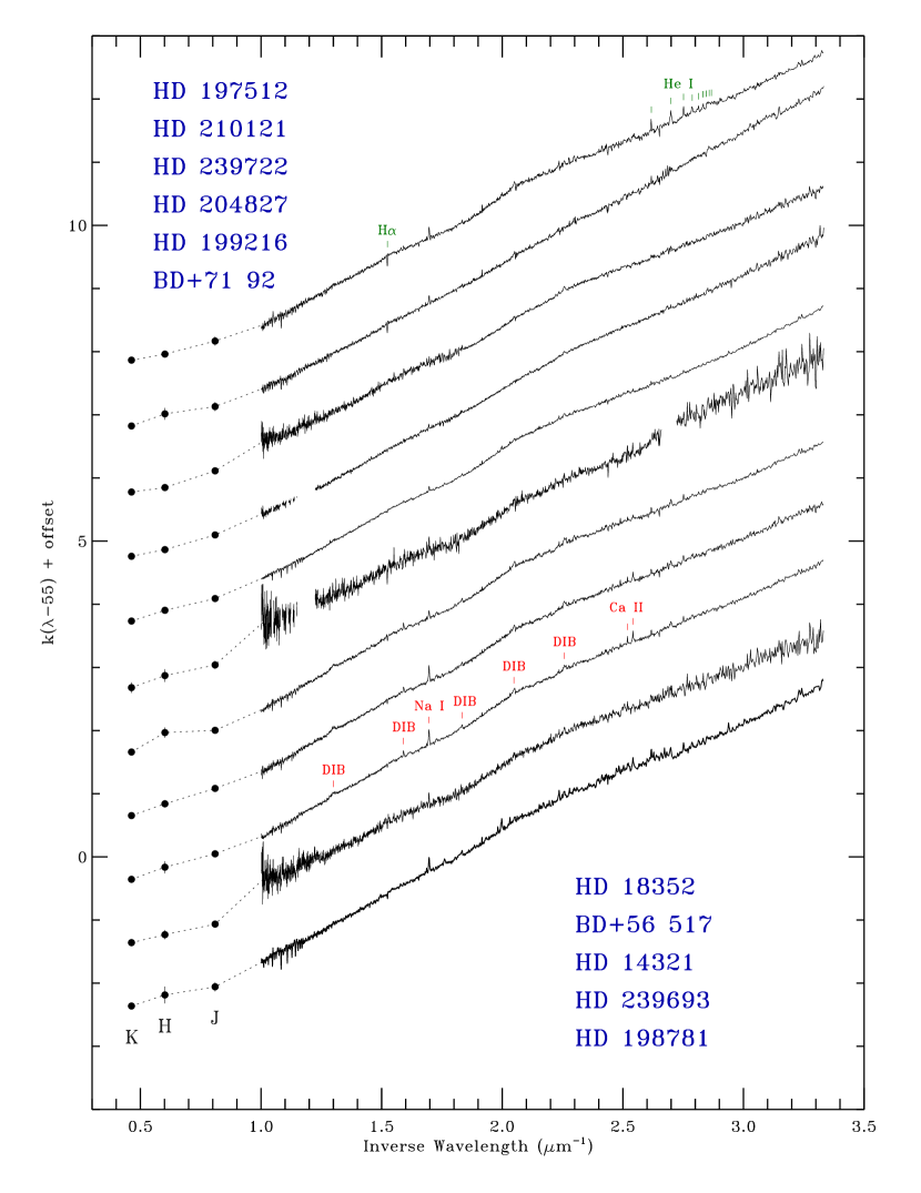
Figure 4a: Normalized NIR-through-optical extinction curves for the program stars, in the form $\mbox{$k(\lambda\!-\!55)$}\/\equiv\mbox{$E(\lambda\!-\!55)$}/\mbox{$E(44\!-\!55)$}$. The large filled circles indicate the extinction in the 2MASS JHK bands. The solid curves show the spectrophotometric extinction curves derived from the HST G430L and G750L data, which are joined at 5450 Å. Narrow features in the curves resulting from stellar spectral mismatch are labeled in green. Interstellar features, including gas-phase absorption lines and diffuse interstellar bands (“DIB”), are labeled in red. Gaps appear in some of the curves near the head of the Paschen series ($\mbox{$\lambda^{-1}$}\simeq 1.2\,\mbox{$\mu{\rm m}^{-1}$}$) and the head of the Balmer series ($\mbox{$\lambda^{-1}$}\simeq\/2.7\,\mbox{$\mu{\rm m}^{-1}$}$) where stellar mismatch features were removed. See the discussion in §3.2. The curves are organized in order of increasing $|k(K\!-\!55)|$, throughout the figures. Arbitrary offsets are added for clarity.

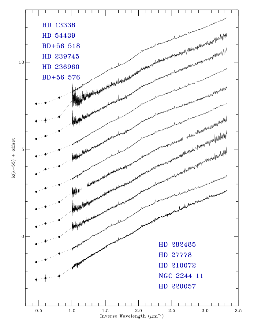
Figure 4b: Same as Figure 4a.

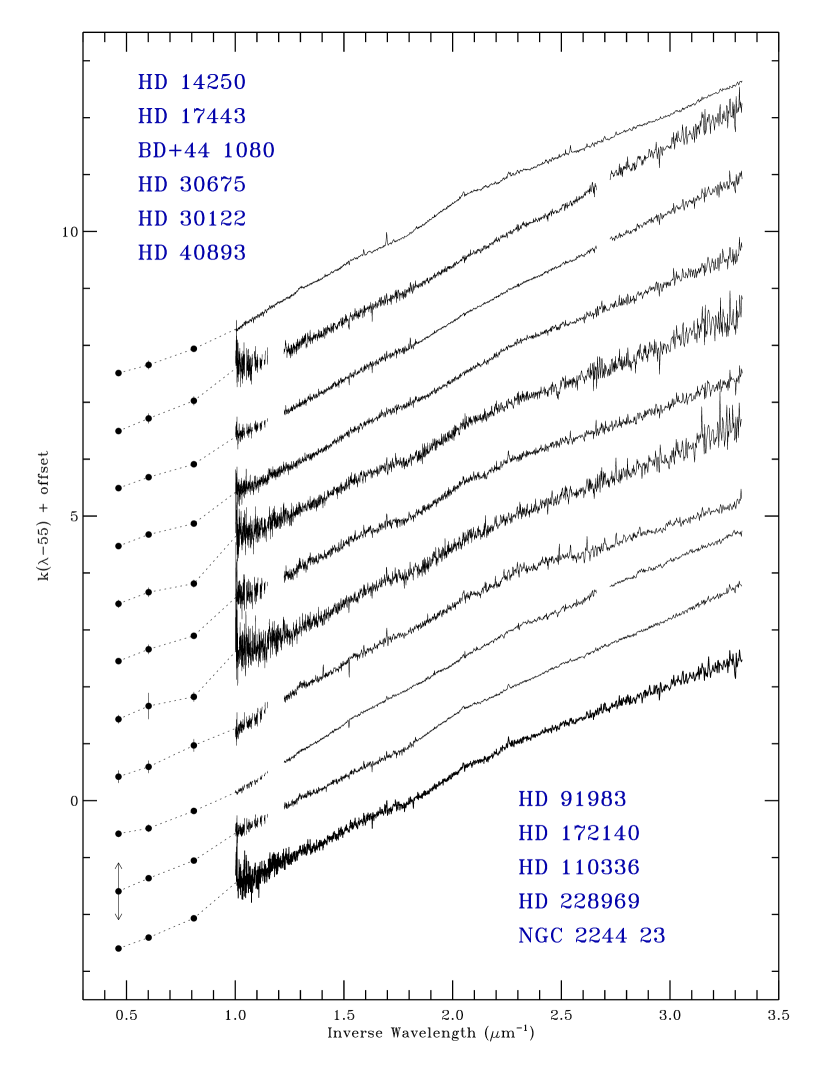
Figure 4c: Same as Figure 4a.

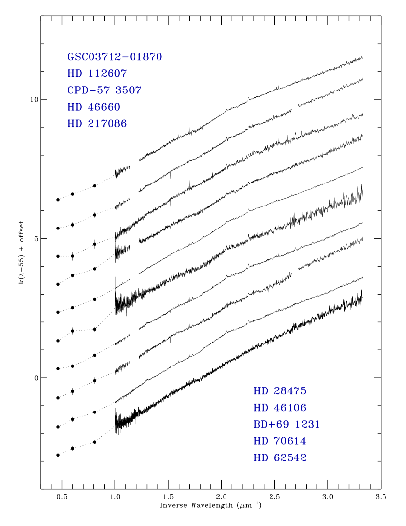
Figure 4d: Same as Figure 4a.

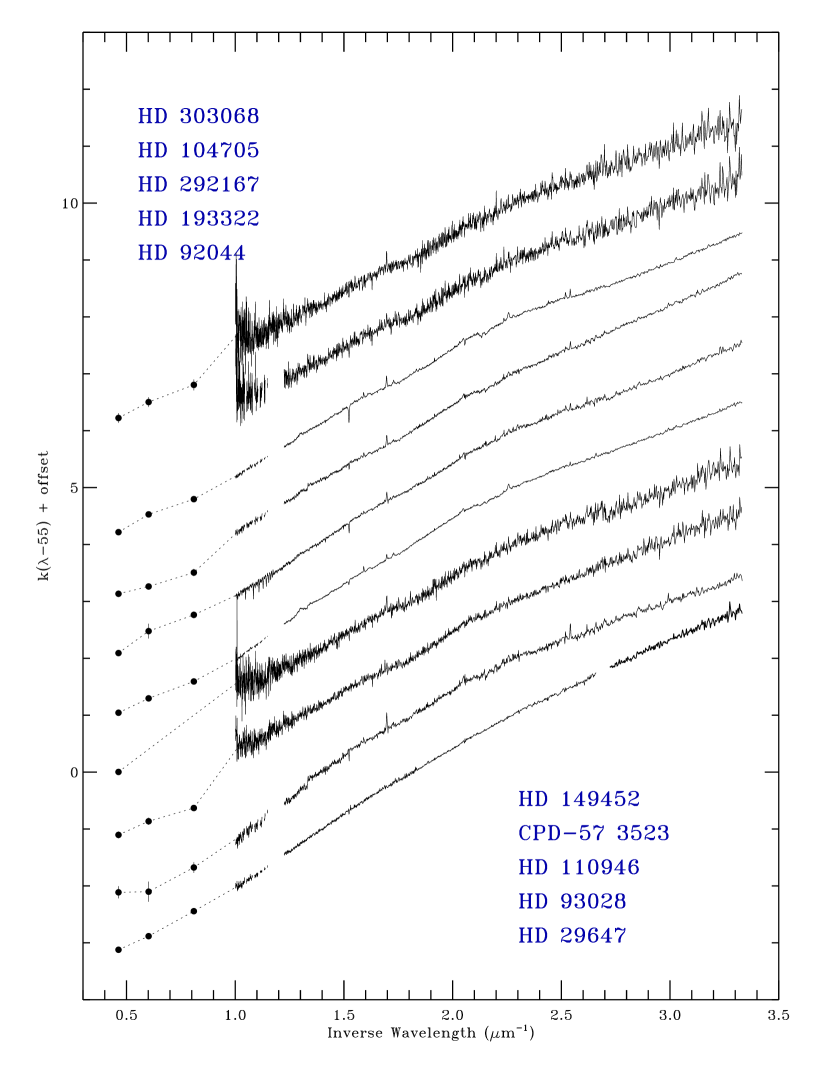
Figure 4e: Same as Figure 4a.

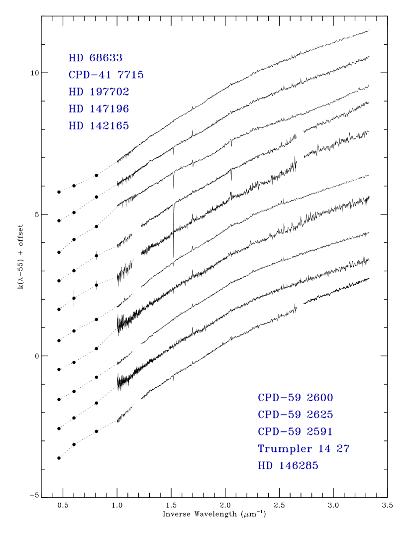
Figure 4f: Same as Figure 4a.

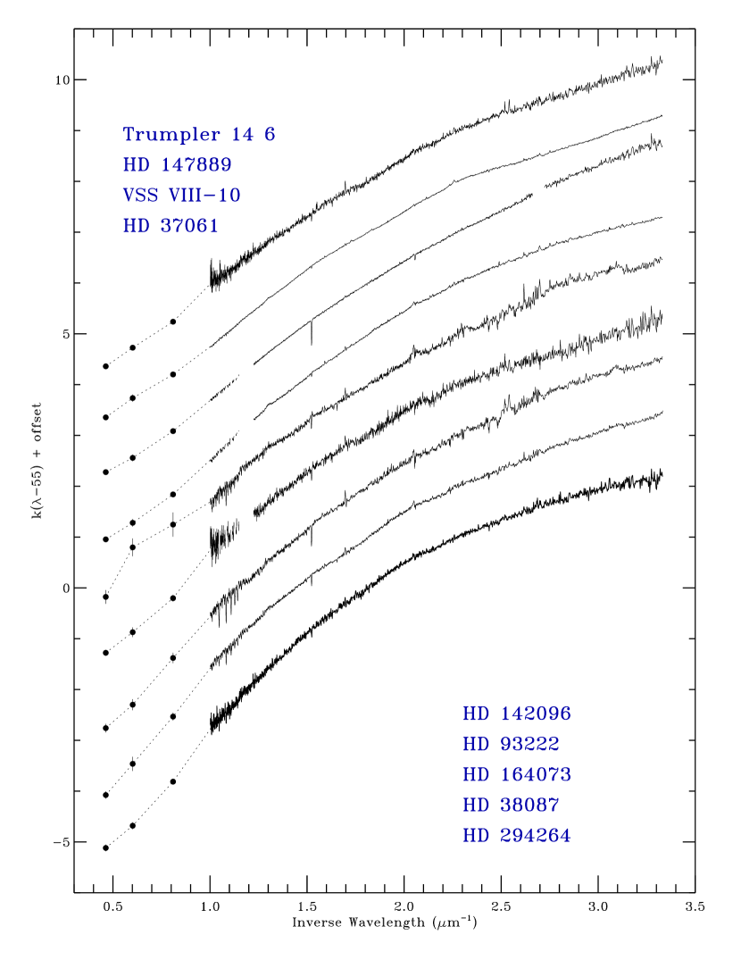
Figure 4g: Same as Figure 4a.

The normalized optical and NIR extinction curves for all 72 of our program stars are shown in Figure 4. The portions of the curves derived from 2MASS JHK data are shown as discrete points at 0.46, 0.62, and 0.81 $\mu{\rm m}^{-1}$, while the portions derived from the combined HST G750L and G430L data are shown from 1.0 $\mu{\rm m}^{-1}$ to 3.33 $\mu{\rm m}^{-1}$. For clarity, the stars are sorted by their $K$-band extinction, with the smallest values of $|k(K-55)|$ at the top of panel 4a and the largest at the bottom of panel 4g. The UV portion of the curves for 71 of the 72 program stars have already been presented in F05 and F07 and, apart from the normalization, there are no substantial differences between the results here and those of the earlier work. There is no previously published UV extinction curve for the heavily reddened O star GSC03712-01870 [$\mbox{$E(B\!-\!V)$}\simeq 1$], located in the direction of – but beyond – the Perseus arm (Muzzio & Rydgren, 1974). Its far-UV curve (i.e., for $\lambda<2000$ Å, since no long wavelength IUE spectra exist) is unremarkable, closely resembling the Milky Way average curve.

A number of the curves in Figure 4 show gaps near 1.2 $\mu{\rm m}^{-1}$ and/or 2.7 $\mu{\rm m}^{-1}$. The SPECTRUM models fail to precisely reproduce the hydrogen lines near the head of the Balmer series (e.g., see Figure 3g) – which is not surprising given the complexity in modeling the overlapping lines – and this produces “mismatch features” in the curves of the coolest stars in our sample. To avoid these distracting features, we eliminated the region between 3670 Å and 3760 Å ($\sim$2.7 $\mu{\rm m}^{-1}$) for these stars from the plots. The cool star models also failed to precisely reproduce the higher Paschen lines of hydrogen and so, likewise, we eliminated the region near 8200 Å ($\sim$1.2 $\mu{\rm m}^{-1}$). The TLUSTY OSTAR2002 models used for the hottest of our stars did not include the individual Paschen features and so the regions near these lines were also eliminated. All other features of the curves are on display in the panels of Figure 4. Some discrete stellar mismatch features still exist in some of the curves, but most of the observed structure – from the narrowest to the broadest scales visible on the plots – is a product of the interstellar medium. The most common and prominent stellar mismatch feature arises from non-photospheric H$\alpha$ emission, which produces a narrow dip in the curves of some of the stars at 6563 Å (1.52 $\mu{\rm m}^{-1}$). This feature is labeled (in green) in the top curve of Figure 4a. Several mismatched stellar He I lines from the $2^{3}P^{0}-n^{3}D$ series are also seen (and labeled in green) in this curve. These absorption lines are stronger in the star (HD 197512) than in the best-fit model and produce narrow spikes in the extinction ++curve. This is not common in our sample and suggests that HD 197512 is a member of the class of helium-strong B stars as seen in the Orion nebula (e.g., Morgan et al., 1978). Narrow features in the curves arising from diffuse interstellar bands (“DIBs,” Herbig, 1975) and interstellar Na I and Ca II absorption are labeled (in red) in panel 4a for the HD 14321 curve.

The collection of spectrophotometric extinction curves in Figure 4 exhibits sightline-to-sightline variability on all scales, ranging from the narrow DIB’s with widths of a fraction of 1 $\mu{\rm m}^{-1}$ to the broadest view-able scales. This largest scale structure can be seen most clearly in a comparison between, for example, the nearly linear curve for HD 210121 in Figure 4a and the nearly quadratic curves for HD 294264 or HD 37061 in Figure 4g. Intermediate scale structure can also be discerned in many of the curves, notably in HD 197512 or HD 199216 in Figure 4a. Generally speaking, this structure resembles a broad dip in the extinction at $\sim$1.6 $\mu{\rm m}^{-1}$ and/or a rise in extinction at $\sim$2 $\mu{\rm m}^{-1}$and corresponds to the “Very Broad Structure” referred to in §1. In a forthcoming paper, Massa et al. (2020) analyze this intermediate scale structure and its variability, and search for relationships with other aspects of NIR through UV extinction. In the remainder of this paper, our focus will be to determine the mean properties of NIR through UV extinction and quantify the broadest scale of sightline-to-sightline variations.

4 Results

4.1 The $R$-dependent Milky Way Extinction Curve

It was first shown by (Cardelli et al., 1989, hereafter CCM) that some large scale properties of UV extinction (particularly, the general level in the far-UV) appear correlated with $R(V)$. This wavelength coherence allows a family of $R(V)$-dependent extinction curves to be derived, potentially reducing the uncertainties in applying extinction corrections to sightlines with measured values of $R(V)$ but otherwise unknown extinction properties. Subsequent studies (e.g., F07) have shown that much of this correlated behavior is driven by a relatively small number of sightlines with extreme values of $R(V)$ and that extinction curves with similar values of $R(V)$ may have a wide range in UV properties (e.g., Mathis & Cardelli, 1992; Valencic et al., 2004). Nevertheless, the $R(V)$-dependence is important since, with appropriate estimation of the uncertainties, it can (1) potentially reduce dereddening errors, (2) allow a meaningful definition of a Milky Way average extinction curve, i.e., as that which corresponds to the mean observed value of $R(V)$, and (3) provide insight into the link between interstellar environment and dust grain properties (see the discussion in Fitzpatrick, 1999).

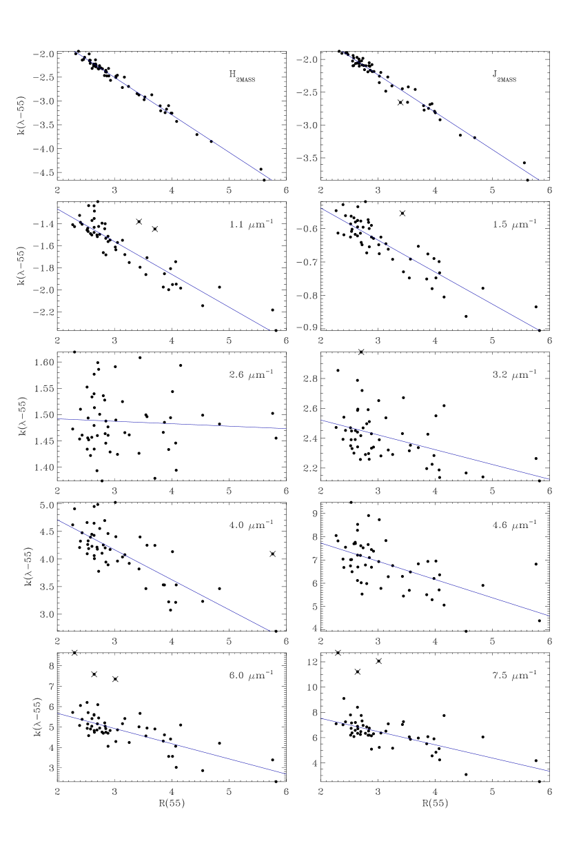
Figure 5: Examples of the $R(55)$-dependence of the normalized extinction curves, where $R(55)\equiv A(55)/\mbox{$E(44\!-\!55)$}$, for the 55 stars in our sample with $E(B-V)>0.30$ (solid symbols). The specific wavelengths shown include the NIR ($H$, $J$ and 1.1 $\mu{\rm m}^{-1}$), optical (1.5, 2.6 and 3.2 $\mu{\rm m}^{-1}$), and UV (4.0, 4.6, 6.0, and 7.5 $\mu{\rm m}^{-1}$) spectral regions. The values of $R(55)$ for each star were determined from Equation 7, as discussed in §4.1. The blue lines show linear fits to $k(\lambda\!-\!55)$ vs. $R(55)$ at each wavelength. Crossed out points were excluded from the fit using a “sigma-clipping” criterion set at 2.5$\sigma$. Fits such as these were performed for each of the 2700 data points defining the full extinction curves.

We examined the $R$-dependence of the curves in our sample in the simplest way, by plotting the values $k(\lambda\!-\!55)$ versus $R$ at each wavelength point in the dataset. We determined values of $R$ for by using the results from F07, who found that – when fitting the NIR data with a power law formula – the values of $R(V)$ were related to the extinction at the $K$ band by the relation:

$$R(V)=-1.19\times k(K-V)-0.26$$ (6)

This can be converted to our normalization system by using the mean transformation in Equation (5), and yields:

$$R(55)=-1.19\times k(K-55)-0.25$$ (7)

Plots of $k(\lambda\!-\!55)$ vs. $R(55)$ are shown in Figure 5 for 10 representative wavelengths (out of a total of 2700 points per curve), spanning the NIR through UV region. The $R(55)$-dependence is noisy but reasonably well defined for most data points. To quantify the relationship, we fit a simple linear function at each wavelength, recording the intercept, slope, and standard deviation about the fit. A single iteration 2.5-$\sigma$ $\sigma$-clip was performed to eliminate extreme points from the fit. In Figure 5, the blue lines show the fits and points that are crossed out indicate those rejected by the $\sigma$-clipping. This procedure was restricted to the 55 sightlines in our sample for which $E(B\!-\!V)$$>0.30$, which minimizes the impact of the larger random errors inherent in the low $E(B\!-\!V)$ curves.

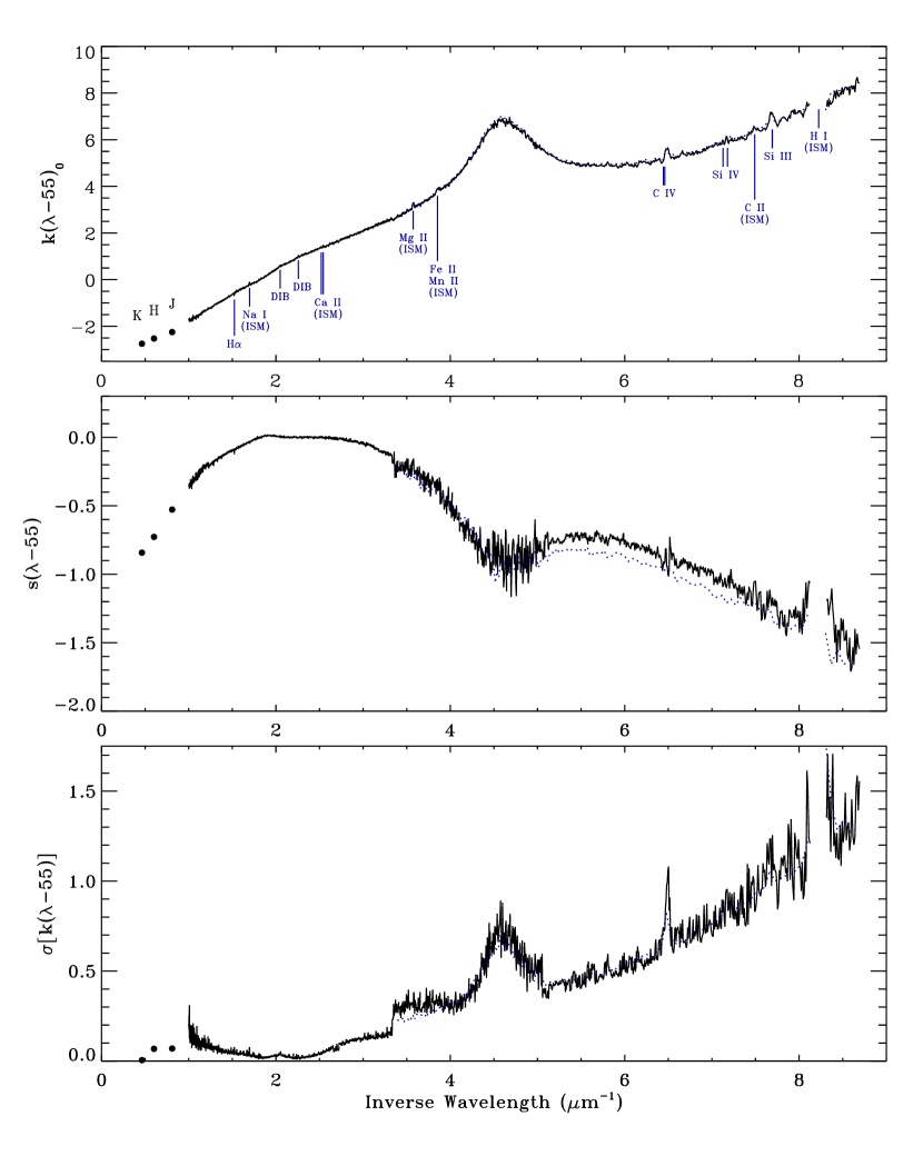
Figure 6: The $R(55)$-Dependent Relationship. Top panel: The mean NIR thru UV extinction curve in the form $\mbox{$k(\lambda\!-\!55)$}_{0}\equiv\mbox{$E(\lambda\!-\!55)$}/\mbox{$E(44\!-\!55)$}$ for the case of $R(55)=3.02$, as derived from the linear fits to $k(\lambda\!-\!55)$ vs. $R(55)$ described in §4.1 and illustrated in Figure 5. This value of $R(55)$ corresponds to $R(V)=3.10$, which is generally considered to be the Milky Way mean. Features in the UV curve due to stellar mismatch, interstellar gas absorption lines, or geocoronal Ly$\alpha$ emission are indicated. Middle panel: The linear dependence of the mean curve on $R(55)$. These values are the slopes of the linear fits described in §4.1. Bottom panel: Standard deviation of the individual curves about the mean $R(55)$-dependence. The dotted blue curves in the UV region of each panel show the results of a similar analysis performed by us on the much larger set of UV extinction curves presented by F07; see the discussion in §5.1.

Figure 6 graphically illustrates the overall results of fitting the linear $R$-dependence in our dataset. The curve in the top panel shows $\mbox{$k(\lambda\!-\!55)$}_{0}$, the values of the fits at $R(55)$ = 3.02, which corresponds to the Milky Way mean value of $R(V)$ = 3.10 (see, Eq. 5). Thus, this curve shows our measurement of the extinction representative of the diffuse ISM over the wavelength range 1150 Å to 2.5 $\mu{\rm m}$. Prominent stellar and interstellar mismatch features are labeled in blue. The middle panel shows the slopes of the fits, $s(\lambda-55)\equiv\Delta$$k(\lambda\!-\!55)$/ $\Delta R(55)$, illustrating the $R(55)$-dependence. The coherence and magnitude of the structure in the $s(\lambda-55)$ plot, as compared to its point-to point scatter, indicate that the fitting procedure has identified a true $R$-dependence in the data, rather than just quantifying the noise. Finally, the bottom panel shows $\sigma[\mbox{$k(\lambda\!-\!55)$}]$, the standard deviation of the individual sightlines against the mean relationship, which quantifies the combination of measurement noise and real deviations from the $R$-dependent relation.

A comparison between the functional dependence of extinction on $R$ adopted here and that used by CCM is given in Appendix B.

4.2 A Tabular Form of the R-dependent Relationship

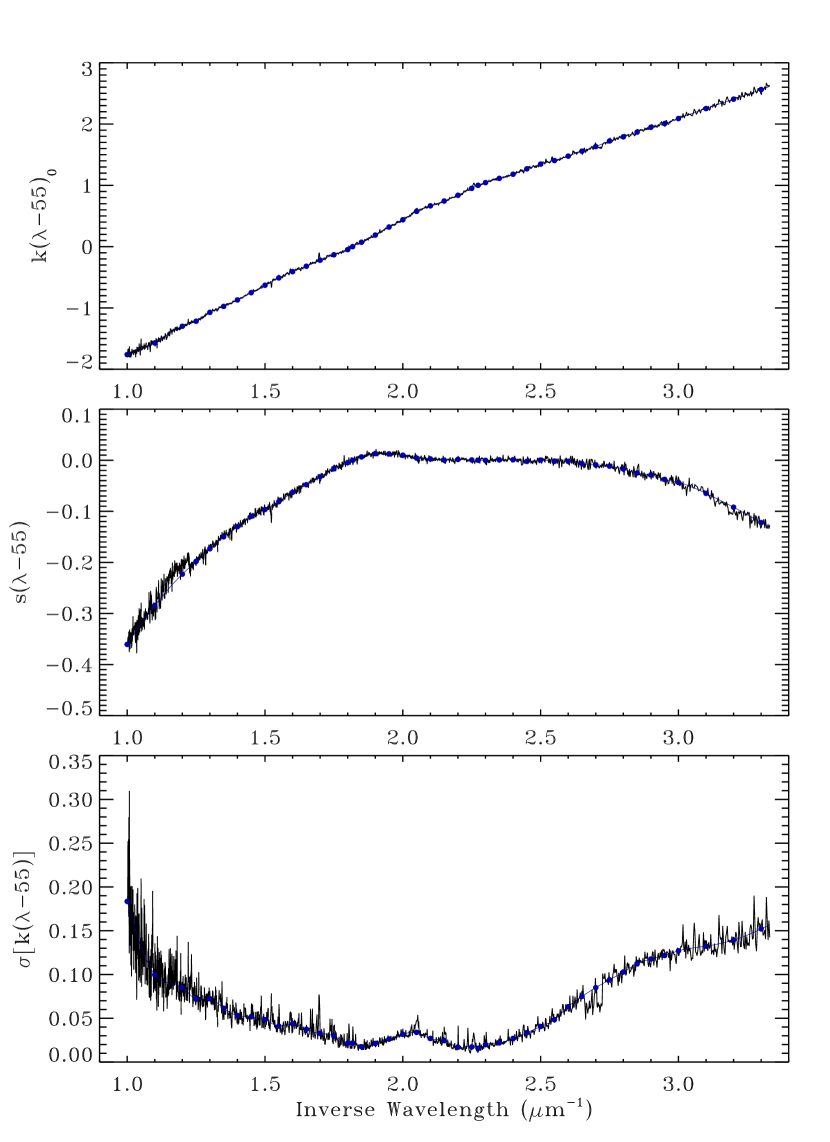
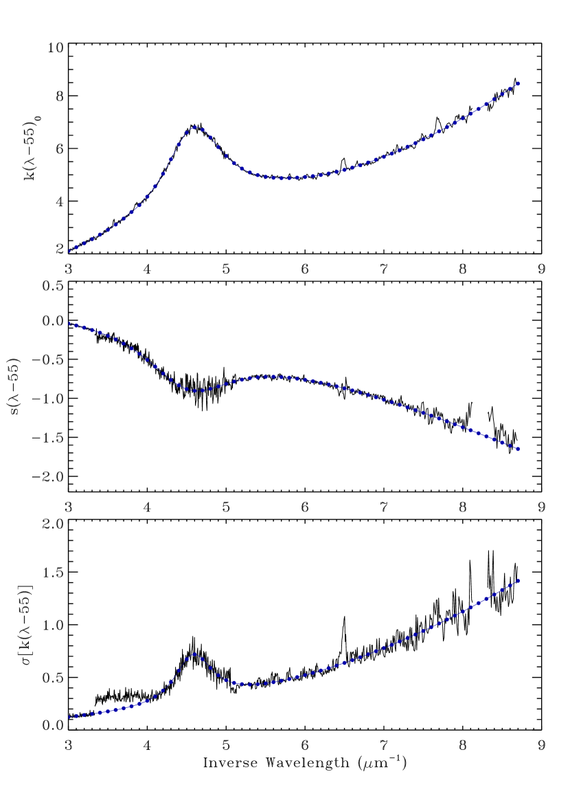
Figure 7: Creating a tabular form of the $R$-dependence of the Milky Way Extinction Curve in the optical/NIR (left) and UV (right) spectral regions. In the optical, a cubic spline was fit to the $k(\lambda\!-\!55)$₀ (top panel), $s(\lambda-55)$ (middle panel), and $\sigma[\mbox{$k(\lambda\!-\!55)$}]$ (bottom panel) curves. The anchor points were spaced at 0.05 $\mu{\rm m}^{-1}$ intervals between 1.2 $\mu{\rm m}^{-1}$ and 3.0 $\mu{\rm m}^{-1}$ and at intervals of 0.1 $\mu{\rm m}^{-1}$ outside that range. The values of the anchors were adjusted iteratively to achieve the best fit to the respective curves. Additional points were added at 1.818 $\mu{\rm m}^{-1}$ (5500 Å) and 2.273 $\mu{\rm m}^{-1}$ (4400 Å) to ensure the normalization. The cubic spline fits are shown by the blue curves and the anchor points are indicated by the filled blue circles. In the UV, the data were fit by variants of the UV fitting functions adopted by F07. The fits are shown by the blue curves and their values at 0.1 $\mu{\rm m}^{-1}$ intervals are shown by the filled blue circles. To assure continuity with the optical results, the UV fits were extended into the optical region (between 3.0 and 3.3 $\mu{\rm m}^{-1}$) and low weight was given to the longest wavelength UV data, due to instability in the calibration of IUE ’s long wavelength camera at these wavelengths. A tabular form of these curves is given in Table 3. See the discussion is §4.2.

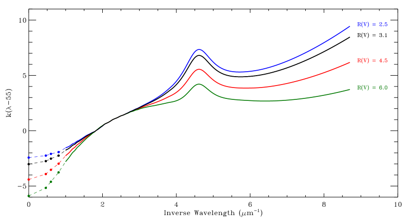
Figure 8: $R(V)$-dependent NIR through UV extinction curves from this study, shown for several values of $R(V)$. The curves were produced from the data in Table 3 using Equation (9).

Table 3: Average Milky Way Extinction Curve

x	$k(\lambda-55)_{0}$	$s(\lambda-55)$	$\sigma[k(\lambda-55)]$			x	$k(\lambda-55)_{0}$	$s(\lambda-55)$	$\sigma[k(\lambda-55)]$
$0.000$	$-3.020$	$-1.000$	$0.000$			$3.700$	$3.337$	$-0.299$	$0.207$
K2MASS	$-2.747$	$-0.842$	$0.000$			$3.800$	$3.586$	$-0.360$	$0.225$
H2MASS	$-2.523$	$-0.727$	$0.068$			$3.900$	$3.849$	$-0.430$	$0.248$
J2MASS	$-2.247$	$-0.528$	$0.069$			$4.000$	$4.169$	$-0.508$	$0.278$
$1.000$	$-1.761$	$-0.361$	$0.184$			$4.100$	$4.562$	$-0.594$	$0.318$
$1.100$	$-1.572$	$-0.284$	$0.100$			$4.200$	$5.039$	$-0.682$	$0.375$
$1.200$	$-1.300$	$-0.223$	$0.085$			$4.300$	$5.589$	$-0.765$	$0.456$
$1.250$	$-1.217$	$-0.198$	$0.072$			$4.400$	$6.151$	$-0.835$	$0.564$
$1.300$	$-1.073$	$-0.173$	$0.072$			$4.500$	$6.603$	$-0.882$	$0.673$
$1.350$	$-0.976$	$-0.150$	$0.061$			$4.600$	$6.804$	$-0.903$	$0.719$
$1.400$	$-0.870$	$-0.130$	$0.053$			$4.700$	$6.712$	$-0.900$	$0.673$
$1.450$	$-0.751$	$-0.110$	$0.052$			$4.800$	$6.416$	$-0.879$	$0.590$
$1.500$	$-0.630$	$-0.096$	$0.048$			$4.900$	$6.053$	$-0.848$	$0.520$
$1.550$	$-0.511$	$-0.081$	$0.041$			$5.000$	$5.716$	$-0.815$	$0.474$
$1.600$	$-0.408$	$-0.063$	$0.044$			$5.100$	$5.443$	$-0.785$	$0.448$
$1.650$	$-0.320$	$-0.048$	$0.037$			$5.200$	$5.237$	$-0.760$	$0.435$
$1.700$	$-0.221$	$-0.032$	$0.033$			$5.300$	$5.089$	$-0.742$	$0.432$
$1.750$	$-0.133$	$-0.017$	$0.030$			$5.400$	$4.989$	$-0.730$	$0.435$
$1.800$	$-0.049$	$-0.005$	$0.022$			$5.500$	$4.925$	$-0.724$	$0.443$
$1.818$	$\phantom{string}0.000$	$\phantom{string}0.000$	$0.022$			$5.600$	$4.889$	$-0.724$	$0.455$
$1.850$	$\phantom{string}0.072$	$\phantom{string}0.007$	$0.017$			$5.700$	$4.875$	$-0.728$	$0.468$
$1.900$	$\phantom{string}0.188$	$\phantom{string}0.013$	$0.021$			$5.800$	$4.876$	$-0.737$	$0.485$
$1.950$	$\phantom{string}0.319$	$\phantom{string}0.012$	$0.026$			$5.900$	$4.891$	$-0.749$	$0.502$
$2.000$	$\phantom{string}0.438$	$\phantom{string}0.010$	$0.032$			$6.000$	$4.916$	$-0.764$	$0.522$
$2.050$	$\phantom{string}0.576$	$\phantom{string}0.004$	$0.034$			$6.100$	$4.949$	$-0.781$	$0.543$
$2.100$	$\phantom{string}0.665$	$\phantom{string}0.003$	$0.027$			$6.200$	$4.993$	$-0.801$	$0.565$
$2.150$	$\phantom{string}0.744$	$\phantom{string}0.000$	$0.024$			$6.300$	$5.049$	$-0.823$	$0.588$
$2.200$	$\phantom{string}0.838$	$\phantom{string}0.002$	$0.017$			$6.400$	$5.115$	$-0.847$	$0.612$
$2.250$	$\phantom{string}0.951$	$\phantom{string}0.001$	$0.017$			$6.500$	$5.190$	$-0.872$	$0.638$
$2.273$	$\phantom{string}1.000$	$\phantom{string}0.000$	$0.016$			$6.600$	$5.273$	$-0.899$	$0.664$
$2.300$	$\phantom{string}1.044$	$-0.000$	$0.020$			$6.700$	$5.365$	$-0.927$	$0.691$
$2.350$	$\phantom{string}1.113$	$\phantom{string}0.001$	$0.022$			$6.800$	$5.465$	$-0.956$	$0.719$
$2.400$	$\phantom{string}1.181$	$\phantom{string}0.001$	$0.027$			$6.900$	$5.571$	$-0.987$	$0.748$
$2.450$	$\phantom{string}1.269$	$-0.002$	$0.034$			$7.000$	$5.685$	$-1.018$	$0.778$
$2.500$	$\phantom{string}1.346$	$\phantom{string}0.000$	$0.041$			$7.100$	$5.805$	$-1.050$	$0.809$
$2.550$	$\phantom{string}1.405$	$-0.002$	$0.048$			$7.200$	$5.932$	$-1.083$	$0.841$
$2.600$	$\phantom{string}1.476$	$-0.002$	$0.063$			$7.300$	$6.065$	$-1.117$	$0.874$
$2.650$	$\phantom{string}1.558$	$-0.006$	$0.075$			$7.400$	$6.203$	$-1.151$	$0.907$
$2.700$	$\phantom{string}1.632$	$-0.009$	$0.085$			$7.500$	$6.347$	$-1.186$	$0.941$
$2.750$	$\phantom{string}1.724$	$-0.012$	$0.094$			$7.600$	$6.497$	$-1.222$	$0.976$
$2.800$	$\phantom{string}1.791$	$-0.017$	$0.103$			$7.700$	$6.652$	$-1.259$	$1.012$
$2.850$	$\phantom{string}1.868$	$-0.025$	$0.112$			$7.800$	$6.812$	$-1.296$	$1.049$
$2.900$	$\phantom{string}1.947$	$-0.029$	$0.118$			$7.900$	$6.978$	$-1.333$	$1.087$
$2.950$	$\phantom{string}2.008$	$-0.037$	$0.122$			$8.000$	$7.148$	$-1.371$	$1.125$
$3.000$	$\phantom{string}2.090$	$-0.043$	$0.127$			$8.100$	$7.323$	$-1.410$	$1.164$
$3.100$	$\phantom{string}2.252$	$-0.065$	$0.132$			$8.200$	$7.502$	$-1.449$	$1.204$
$3.200$	$\phantom{string}2.406$	$-0.092$	$0.139$			$8.300$	$7.686$	$-1.488$	$1.245$
$3.300$	$\phantom{string}2.563$	$-0.122$	$0.152$			$8.400$	$7.874$	$-1.528$	$1.287$
$3.400$	$\phantom{string}2.728$	$-0.160$	$0.165$			$8.500$	$8.067$	$-1.568$	$1.329$
$3.500$	$\phantom{string}2.911$	$-0.200$	$0.177$			$8.600$	$8.264$	$-1.609$	$1.373$
$3.600$	$\phantom{string}3.112$	$-0.245$	$0.191$			$8.700$	$8.464$	$-1.650$	$1.417$

To make the new results in Figure 6 useful for other extinction investigations, we created a tabular form of these data. This was done by fitting the three curves in Figure 6 with smooth functions and then recording the values of the functions at selected wavelengths. The details of this process are illustrated in Figure 7 where the smooth blue curves show the fits to the data and the blue circles indicate the selected points.

In the optical/NIR, i.e., for the HST spectrophotometric data, we fit cubic splines to the three curves, with anchor points spaced every 0.1 $\mu{\rm m}^{-1}$in the interval 1.0 $\mu{\rm m}^{-1}$ (10000 Å) to 3.3 $\mu{\rm m}^{-1}$ (3030 Å), with intermediate points added between 1.2 $\mu{\rm m}^{-1}$ and 2.9 $\mu{\rm m}^{-1}$ and two special points – at 1.818 $\mu{\rm m}^{-1}$(5500 Å) and 2.273 $\mu{\rm m}^{-1}$(4400 Å) – added to enforce the normalization. Regions near the Balmer and Paschen jumps that are affected by spectral mismatch were given zero weight so that the fits passed smoothly through these regions in the $s(\lambda-V)$ and $\sigma$[$k(\lambda\!-\!55)$] curves. Likewise, data affected by interstellar absorption features (including DIB’s) and stellar mismatch features were given zero weight. Notice that the values of $\sigma$[$k(\lambda\!-\!55)$] do not go to zero at the normalization points. This is because (as noted in §3.2) the normalization was performed using interpolation within a bin containing the normalization wavelengths. Thus, these small values of $\sigma$[$k(\lambda\!-\!55)$] $\simeq$ 0.02 reflect the point-to-point scatter in the normalization regions of the curves, rather than sightline-to-sightline variations. The large values of $\sigma$[$k(\lambda\!-\!55)$] at the longest optical wavelengths are likely dominated by statistical noise in the HST G750L data rather than curve-to-curve variability. The true curve-to-curve scatter is probably at the level of $\sigma$[$k(\lambda\!-\!55)$] $\simeq$ 0.1, similar to the shorter wavelength G750L data and the 2MASS $J$ and $H$ values.

In the UV, we used variations of the F07 fitting function to achieve smooth representations of the curves. The fits were performed over the wavelength range of the IUE data, i.e., 3.3 $\mu{\rm m}^{-1}$(3030 Å) to 8.7 $\mu{\rm m}^{-1}$ (1150 Å), plus a small section of the HST data, from 3.0 to 3.3 $\mu{\rm m}^{-1}$, which was included to assure continuity with the optical region. Spectral mismatch features were given zero weight in the fits. Figures 6 and 7 show that there is a significant discontinuity between the longest UV wavelengths and the shortest optical wavelengths in the $\sigma$[$k(\lambda\!-\!55)$] curves. We attribute this to instability in the calibration of IUE’s LWR and LWP cameras at their longest wavelengths, where the camera sensitivities are highly dependent on the placement of the spectra on the camera face. We gave the longest UV wavelengths zero weight so that the fits would join smoothly with the optical HST data. There is also a small discontinuity noticeable in $\sigma$[$k(\lambda\!-\!55)$] at the joint between IUE’s short and long wavelength cameras at 5.05 $\mu{\rm m}^{-1}$ (1980 Å) where, once again, the extreme sensitivity of the long wavelength cameras to spectrum placement (and the lower general sensitivity of the cameras) manifests as enhanced scatter. Values of the fits at 0.1 $\mu{\rm m}^{-1}$ intervals over the range 3.3 $\mu{\rm m}^{-1}$ to 8.7 $\mu{\rm m}^{-1}$, as indicated by the filled circles in Figure 7, were recorded.

The final tabular form of our extinction results are given in Table 3. The columns in the table list the wavelengths (in $\mu{\rm m}^{-1}$), followed by the values of $k(\lambda\!-\!55)$₀, $s(\lambda-55)$ and $\sigma[\mbox{$k(\lambda\!-\!55)$}]$. For the spectrophotometric data, these all correspond to the filled circles in Figure 7. For the 2MASS $JHK$ data, the values in the table are simply those shown in Figure 6. The result that $\sigma[k(K-55)]=0$ arises because our values of $R(55)$ are tied directly to the $K$-band measurement via Equation (7).

The data in Table 3 can be used to reconstruct an extinction curve in the form of $k(\lambda\!-\!55)$ over the indicated wavelength range for any value of $R(55)$ or $R(V)$ ranging from 2.5 to 6.0. The restriction on the range of valid $R$ values comes directly from the range of $R$ in our data (see Figure 5). The curve can be constructed using the formula:

$$\scriptsize k(\lambda-55)_{R(55)}=k(\lambda-55)_{0}+s(\lambda-55)\times[R(55)-R(55)_{0}]$$ (8)

where $R(55)_{0}=3.02$ and $k(\lambda-55)_{0}$ is the extinction for the case $R(55)=R(55)_{0}$. If $R$ is expressed in $R(V)$ notation, then Equation (8) transforms to:

$$\scriptsize k(\lambda-55)_{R(V)}=k(\lambda-55)_{0}+s(\lambda-55)\times[R(V)-3.10]\times 0.99$$ (9)

Four examples of extinction curves constructed from Table 3 are shown in Figure 8, for values of $R(V)$ = 2.5, 3.1, 4.5, and 6.0. The $R$-dependent extinction relationship is available in the dust_extinction python package as the “F20” model.

4.3 Reddening Slopes for Optical Photometry

Given the advent of large ground-based surveys and the overall prevalence of the data, optical photometry remains a powerful astronomical tool. Knowledge of the effects of interstellar extinction on the various photometric systems is important for disentangling the intrinsic and extrinsic (i.e., interstellar) contributions to photometric measurements.

Table 4: UBV and uvby Extinction Indices

$T_{eff}$		$\frac{E(B-V)}{E(44-55)}$	$\frac{E(U-B)}{E(B-V)}$	$\frac{E(b-y)}{E(B-V)}$	$\frac{E(m_{1})}{E(b-y)}$	$\frac{E(c_{1})}{E(b-y)}$			$\frac{E(B-V)}{E(44-55)}$	$\frac{E(U-B)}{E(B-V)}$	$\frac{E(b-y)}{E(B-V)}$	$\frac{E(m_{1})}{E(b-y)}$	$\frac{E(c_{1})}{E(b-y)}$
		$R(V)=2.5$
		E(44-55) = 0.50							E(44-55) = 1.00
$7000$K		$0.945$	$0.806$	$0.752$	$-0.299$	$0.285$			$0.933$	$0.830$	$0.762$	$-0.299$	$0.279$
$8000$K		$0.955$	$0.760$	$0.746$	$-0.300$	$0.289$			$0.943$	$0.782$	$0.755$	$-0.301$	$0.283$
$9000$K		$0.964$	$0.730$	$0.738$	$-0.300$	$0.290$			$0.953$	$0.750$	$0.747$	$-0.300$	$0.283$
$10000$K		$0.972$	$0.718$	$0.732$	$-0.297$	$0.290$			$0.961$	$0.739$	$0.740$	$-0.298$	$0.283$
$12500$K		$0.981$	$0.736$	$0.725$	$-0.295$	$0.293$			$0.970$	$0.755$	$0.733$	$-0.295$	$0.287$
$15000$K		$0.985$	$0.752$	$0.722$	$-0.294$	$0.296$			$0.974$	$0.771$	$0.730$	$-0.295$	$0.290$
$20000$K		$0.990$	$0.765$	$0.718$	$-0.293$	$0.299$			$0.979$	$0.784$	$0.726$	$-0.294$	$0.293$
$25000$K		$0.993$	$0.773$	$0.716$	$-0.292$	$0.300$			$0.982$	$0.791$	$0.724$	$-0.292$	$0.294$
$30000$K		$0.996$	$0.775$	$0.713$	$-0.291$	$0.301$			$0.985$	$0.794$	$0.722$	$-0.291$	$0.295$
$35000$K		$0.997$	$0.778$	$0.712$	$-0.290$	$0.301$			$0.986$	$0.796$	$0.721$	$-0.291$	$0.295$
		$R(V)=3.1$
		E(44-55) = 0.50							E(44-55) = 1.00
$7000$K		$0.951$	$0.793$	$0.748$	$-0.301$	$0.263$			$0.940$	$0.815$	$0.756$	$-0.301$	$0.258$
$8000$K		$0.959$	$0.748$	$0.742$	$-0.302$	$0.266$			$0.949$	$0.769$	$0.750$	$-0.303$	$0.261$
$9000$K		$0.968$	$0.718$	$0.735$	$-0.301$	$0.267$			$0.959$	$0.738$	$0.743$	$-0.302$	$0.262$
$10000$K		$0.976$	$0.707$	$0.729$	$-0.299$	$0.267$			$0.966$	$0.727$	$0.736$	$-0.300$	$0.261$
$12500$K		$0.985$	$0.724$	$0.722$	$-0.297$	$0.270$			$0.975$	$0.743$	$0.730$	$-0.297$	$0.264$
$15000$K		$0.989$	$0.739$	$0.719$	$-0.296$	$0.273$			$0.979$	$0.758$	$0.727$	$-0.296$	$0.267$
$20000$K		$0.994$	$0.752$	$0.716$	$-0.295$	$0.276$			$0.984$	$0.770$	$0.723$	$-0.295$	$0.270$
$25000$K		$0.997$	$0.759$	$0.713$	$-0.293$	$0.276$			$0.987$	$0.777$	$0.720$	$-0.294$	$0.271$
$30000$K		$0.999$	$0.761$	$0.711$	$-0.293$	$0.277$			$0.990$	$0.779$	$0.718$	$-0.293$	$0.271$
$35000$K		$1.001$	$0.764$	$0.710$	$-0.292$	$0.277$			$0.991$	$0.782$	$0.717$	$-0.292$	$0.272$
		$R(V)=4.5$
		E(44-55) = 0.50							E(44-55) = 1.00
$7000$K		$0.964$	$0.761$	$0.739$	$-0.305$	$0.211$			$0.958$	$0.780$	$0.744$	$-0.306$	$0.207$
$8000$K		$0.971$	$0.720$	$0.734$	$-0.306$	$0.214$			$0.965$	$0.738$	$0.739$	$-0.307$	$0.210$
$9000$K		$0.979$	$0.692$	$0.728$	$-0.305$	$0.214$			$0.973$	$0.709$	$0.733$	$-0.306$	$0.211$
$10000$K		$0.986$	$0.682$	$0.722$	$-0.303$	$0.214$			$0.980$	$0.699$	$0.727$	$-0.304$	$0.210$
$12500$K		$0.994$	$0.696$	$0.716$	$-0.300$	$0.216$			$0.989$	$0.713$	$0.720$	$-0.301$	$0.212$
$15000$K		$0.998$	$0.710$	$0.713$	$-0.300$	$0.218$			$0.992$	$0.726$	$0.718$	$-0.301$	$0.214$
$20000$K		$1.002$	$0.721$	$0.710$	$-0.298$	$0.220$			$0.997$	$0.737$	$0.714$	$-0.299$	$0.217$
$25000$K		$1.005$	$0.728$	$0.708$	$-0.297$	$0.221$			$0.999$	$0.744$	$0.712$	$-0.298$	$0.217$
$30000$K		$1.007$	$0.730$	$0.706$	$-0.296$	$0.221$			$1.002$	$0.746$	$0.710$	$-0.297$	$0.217$
$35000$K		$1.008$	$0.732$	$0.705$	$-0.296$	$0.222$			$1.003$	$0.748$	$0.710$	$-0.297$	$0.218$
		$R(V)=6.0$
		E(44-55) = 0.50							E(44-55) = 1.00
$7000$K		$0.978$	$0.728$	$0.729$	$-0.309$	$0.155$			$0.979$	$0.743$	$0.729$	$-0.310$	$0.153$
$8000$K		$0.983$	$0.690$	$0.725$	$-0.310$	$0.158$			$0.983$	$0.705$	$0.726$	$-0.312$	$0.155$
$9000$K		$0.990$	$0.664$	$0.720$	$-0.309$	$0.158$			$0.990$	$0.678$	$0.721$	$-0.311$	$0.155$
$10000$K		$0.997$	$0.654$	$0.715$	$-0.307$	$0.156$			$0.997$	$0.668$	$0.716$	$-0.309$	$0.154$
$12500$K		$1.004$	$0.667$	$0.709$	$-0.305$	$0.158$			$1.004$	$0.681$	$0.710$	$-0.306$	$0.155$
$15000$K		$1.008$	$0.679$	$0.707$	$-0.304$	$0.159$			$1.008$	$0.692$	$0.708$	$-0.305$	$0.157$
$20000$K		$1.012$	$0.688$	$0.704$	$-0.303$	$0.161$			$1.011$	$0.702$	$0.705$	$-0.304$	$0.159$
$25000$K		$1.014$	$0.694$	$0.702$	$-0.301$	$0.161$			$1.014$	$0.708$	$0.703$	$-0.303$	$0.159$
$30000$K		$1.016$	$0.695$	$0.700$	$-0.301$	$0.161$			$1.016$	$0.709$	$0.701$	$-0.302$	$0.159$
$35000$K		$1.017$	$0.697$	$0.700$	$-0.300$	$0.161$			$1.017$	$0.711$	$0.701$	$-0.301$	$0.159$

Table 5: ugriz Extinction Indices

$T_{eff}$		$\frac{E(u-g)}{E(44-55)}$	$\frac{E(g-r)}{E(44-55)}$	$\frac{E(r-i)}{E(44-55)}$	$\frac{E(i-z)}{E(44-55)}$			$\frac{E(u-g)}{E(44-55)}$	$\frac{E(g-r)}{E(44-55)}$	$\frac{E(r-i)}{E(44-55)}$	$\frac{E(i-z)}{E(44-55)}$
		$R(V)=2.5$
		E(44-55) = 0.50						E(44-55) = 1.00
$7000$K		$1.101$	$1.000$	$0.562$	$0.433$			$1.114$	$0.979$	$0.560$	$0.433$
$8000$K		$1.072$	$1.014$	$0.565$	$0.436$			$1.085$	$0.992$	$0.563$	$0.436$
$9000$K		$1.054$	$1.028$	$0.567$	$0.438$			$1.067$	$1.006$	$0.565$	$0.438$
$10000$K		$1.049$	$1.036$	$0.567$	$0.438$			$1.063$	$1.014$	$0.565$	$0.438$
$12500$K		$1.068$	$1.045$	$0.567$	$0.437$			$1.082$	$1.022$	$0.565$	$0.436$
$15000$K		$1.082$	$1.049$	$0.567$	$0.435$			$1.096$	$1.026$	$0.565$	$0.435$
$20000$K		$1.094$	$1.055$	$0.567$	$0.434$			$1.108$	$1.032$	$0.565$	$0.434$
$25000$K		$1.101$	$1.058$	$0.567$	$0.434$			$1.116$	$1.035$	$0.565$	$0.433$
$30000$K		$1.104$	$1.062$	$0.567$	$0.433$			$1.118$	$1.038$	$0.565$	$0.433$
$35000$K		$1.106$	$1.065$	$0.566$	$0.433$			$1.121$	$1.041$	$0.564$	$0.433$
		$R(V)=3.1$
		E(44-55) = 0.50						E(44-55) = 1.00
$7000$K		$1.087$	$1.037$	$0.622$	$0.502$			$1.101$	$1.018$	$0.619$	$0.503$
$8000$K		$1.059$	$1.051$	$0.625$	$0.506$			$1.073$	$1.031$	$0.623$	$0.506$
$9000$K		$1.041$	$1.064$	$0.627$	$0.508$			$1.055$	$1.044$	$0.624$	$0.508$
$10000$K		$1.036$	$1.072$	$0.627$	$0.508$			$1.050$	$1.051$	$0.625$	$0.508$
$12500$K		$1.053$	$1.081$	$0.627$	$0.506$			$1.068$	$1.060$	$0.624$	$0.506$
$15000$K		$1.067$	$1.085$	$0.627$	$0.504$			$1.082$	$1.064$	$0.624$	$0.504$
$20000$K		$1.078$	$1.091$	$0.627$	$0.503$			$1.094$	$1.069$	$0.624$	$0.503$
$25000$K		$1.085$	$1.094$	$0.627$	$0.502$			$1.100$	$1.072$	$0.625$	$0.502$
$30000$K		$1.087$	$1.097$	$0.627$	$0.502$			$1.103$	$1.075$	$0.625$	$0.502$
$35000$K		$1.090$	$1.100$	$0.626$	$0.502$			$1.105$	$1.078$	$0.623$	$0.502$
		$R(V)=4.5$
		E(44-55) = 0.50						E(44-55) = 1.00
$7000$K		$1.055$	$1.125$	$0.760$	$0.664$			$1.071$	$1.110$	$0.758$	$0.666$
$8000$K		$1.028$	$1.137$	$0.764$	$0.668$			$1.043$	$1.121$	$0.761$	$0.670$
$9000$K		$1.010$	$1.149$	$0.766$	$0.671$			$1.026$	$1.133$	$0.763$	$0.673$
$10000$K		$1.005$	$1.157$	$0.766$	$0.671$			$1.021$	$1.141$	$0.763$	$0.673$
$12500$K		$1.020$	$1.165$	$0.766$	$0.668$			$1.036$	$1.149$	$0.763$	$0.670$
$15000$K		$1.032$	$1.169$	$0.766$	$0.666$			$1.049$	$1.152$	$0.763$	$0.667$
$20000$K		$1.042$	$1.174$	$0.766$	$0.664$			$1.059$	$1.157$	$0.763$	$0.665$
$25000$K		$1.048$	$1.177$	$0.766$	$0.662$			$1.065$	$1.160$	$0.763$	$0.664$
$30000$K		$1.049$	$1.180$	$0.766$	$0.661$			$1.067$	$1.163$	$0.763$	$0.663$
$35000$K		$1.051$	$1.184$	$0.764$	$0.662$			$1.069$	$1.166$	$0.761$	$0.663$
		$R(V)=6.0$
		E(44-55) = 0.50						E(44-55) = 1.00
$7000$K		$1.021$	$1.220$	$0.909$	$0.838$			$1.038$	$1.211$	$0.906$	$0.843$
$8000$K		$0.994$	$1.230$	$0.913$	$0.844$			$1.011$	$1.220$	$0.910$	$0.849$
$9000$K		$0.977$	$1.241$	$0.915$	$0.847$			$0.994$	$1.231$	$0.912$	$0.852$
$10000$K		$0.971$	$1.248$	$0.916$	$0.846$			$0.989$	$1.238$	$0.913$	$0.851$
$12500$K		$0.984$	$1.256$	$0.915$	$0.842$			$1.002$	$1.245$	$0.912$	$0.847$
$15000$K		$0.995$	$1.260$	$0.915$	$0.839$			$1.013$	$1.249$	$0.912$	$0.844$
$20000$K		$1.003$	$1.265$	$0.915$	$0.837$			$1.021$	$1.253$	$0.912$	$0.841$
$25000$K		$1.007$	$1.267$	$0.915$	$0.835$			$1.026$	$1.256$	$0.912$	$0.839$
$30000$K		$1.008$	$1.270$	$0.915$	$0.834$			$1.027$	$1.259$	$0.912$	$0.838$
$35000$K		$1.010$	$1.274$	$0.913$	$0.834$			$1.029$	$1.262$	$0.910$	$0.839$

To illustrate and quantify the effects of interstellar extinction on optical SEDs, we have computed the photometric reddening slopes predicted by our new optical extinction curve for three common photometric systems: Johnson UBV, Strömgren uvby, and Sloan Digital Sky Survey (SDSS) ugriz. The slopes were determined by performing synthetic photometry on intrinsic and reddened stellar energy distributions, using the ATLAS9 atmosphere models, and then forming the various differences and ratios. The results are presented in Tables 4 and 5. The measurements were made for two values of reddening [$E(44\!-\!55)$ = 0.50 and 1.0], four values of $R(V)$ (2.5, 3.1, 4.5, and 6.0), and ten values of $T_{\rm eff}$ (from 7000 K to 35000 K). The synthetic Johnson and Strömgren photometry was performed as described by Fitzpatrick & Massa (2005b). We modified the calibration of the synthetic values, however, to take advantage of the new HST G430L and G750L observations obtained for this program. In brief, we computed synthetic, uncalibrated Johnson and Strömgren photometric indices ($B-V$, $U-B$, $b-y$, $m_{1}$ and $c_{1}$) using the HST spectrophotometry for each of our 72 reddened stars, plus three additional unreddened stars HD 38666, HD 34816, and HD 214680 from the HST archives. We then determined the linear transformation between these synthetic values and the observed photometric indices. The results are similar to those reported in Fitzpatrick & Massa (2005b) and the scatter of the observed values about the synthetic results is consistent with the expected observational error. The synthetic ugriz photometry was performed as described in Casagrande & VandenBerg (2014), with filter profiles from Doi et al. (2010).

The $E(B\!-\!V)$/$E(44\!-\!55)$ column in Table 4 illustrates the uncertainty in measuring the “amount” of extinction using broadband photometry. For a fixed extinction [as measured by $E(44\!-\!55)$], the observed values of $E(B\!-\!V)$ can vary significantly depending on the stellar $T_{\rm eff}$, reflecting variations in the effective wavelengths of the broad $B$ and $V$ filters. For the same reason, the values of $E(B\!-\!V)$/$E(44\!-\!55)$ also depend on the overall level of extinction. The Johnson and Strömgren reddening slopes implied by the $R(V)=3.1$ curve are – with the exception of E(c₁)/$E(B\!-\!V)$ – consistent with the accepted values (see Fitzpatrick, 1999), including the $E(B\!-\!V)$-dependence of $E(U\!-\!B)$/$E(B\!-\!V)$ (e.g., Fitzgerald, 1970). The accepted E(c₁)/$E(B\!-\!V)$ ratio ($\simeq 0.20$) is from Crawford (1975) and based on an “eye fit” to photometry of $\sim$50 O-type stars. However, it is clear from Crawford’s Figure 4 that a steeper ratio is needed to explain the most heavily reddened O stars in the sample. In addition, Crawford notes that a preliminary study of B-type stars yields a larger value ($\simeq 0.24$). We suggest that the results in Table 4 present the most reliable estimates for the Strömgren reddening slopes. Note also that, while the intermediate-bandwidth Strömgren slopes are relatively insensitive to effective wavelength shifts [i.e., minimal dependence on $T_{\rm eff}$ or $E(44\!-\!55)$], the $E(c_{1})$ ratio is strongly dependent on $R(V)$ due to the short wavelength $u$ filter. The same sensitivity is also seen in the $E(U\!-\!B)$ slope, potentially allowing both indices to be used as diagnostics of $R(V)$.

Qualitatively similar effects, in terms of $T_{\rm eff}$ and $E(44\!-\!55)$ sensitivity, can be seen in the ugriz results in Table 5. Note that the reddening slopes involving the longer wavelength riz filters ($\lambda_{\rm eff}$ = 6231, 7625 and 9134 Å, respectively) are particularly sensitive to the values of $R(V)$. Given that there is less curve-to-curve scatter relative to the $R$-correlation at these longer wavelengths (see Figure 7), as compared to that for the Strömgren $u$ or Johnson $U$ filters, these filters could provide a very strong diagnostic of $R(V)$.

4.4 Balmer Decrement

The formation rate of massive stars in external galaxies can be inferred from the luminosities of emission lines – notably, the Balmer lines – arising in the galaxies’ H II regions (e.g., Kennicutt, 1983; Gallagher et al., 1984). This requires that the line emission first be corrected for the attenuating effects of interstellar extinction. A common technique is to compare the observed luminosity ratio of two lines, e.g., $H\alpha/H\beta$, to the expected intrinsic ratio and interpret any difference as a result of the wavelength-dependent effects of reddening. This is the “Balmer Decrement” method and allows an estimate of $E(B\!-\!V)$, which further allows an estimate of the total extinction at the line wavelengths (e.g., Calzetti et al., 1994). This process requires an understanding of the intrinsic emission mechanism and, apropos to this paper, a well-determined interstellar extinction law.

Using the results in Table 3 and following the derivation in, for example, §3 of Domínguez et al. (2013), we can compute the implied reddening based on any pair of lines for which the intrinsic ratio is known. Two examples are:

$$\scriptsize E(44-55)=\frac{2.5}{1.16+0.09\times(R_{55}-3.02)}\times\rm{log}_{10}\left[\frac{(H\alpha/H\beta)_{obs}}{(H\alpha/H\beta)_{int}}\right]$$ (10)

and

$$\scriptsize E(44-55)=-5.43\times\rm{log}_{10}\left[\frac{(H\gamma/H\beta)_{obs}}{(H\gamma/H\beta)_{int}}\right]\>.$$ (11)

In both cases, the subscripts “obs” and “int” refer to the observed line ratios and the expected intrinsic ratios, respectively. Equations (10) and (11) show that the observed ratio is slightly sensitive to the value of $R$ for the H$\alpha$ case, and not at all for the H$\gamma$ case. The overall weakness of the $R$-dependence is because the emission lines lie within or close to the region where the curves are normalized and, therefore, highly constrained.

For the case of the average Milky Way value of $R(55)$ = 3.02 (i.e., $R(V)=3.10$), the constant term in Equation (10) becomes 2.15. To find $E(B\!-\!V)$, this value is reduced by a factor of $\sim$0.99 (see Table 4), yielding a scale factor of 2.13. This can be compared with the value of 1.97 as computed by Domínguez et al. (2013) using the attenuation law of Calzetti et al. (2000), which characterizes regions of starburst activity. Given the difference in the environments involved (Milky Way average vs. starburst), this level of disagreement might be considered unsurprising. However, a closer look shows that it actually reveals a significant problem; namely that the Calzetti et al. (2000) law is not rigorously normalized to the $BV$ system. This is a common problem among most current representations of optical extinction and will be graphically illustrated below in §5.1. In brief, the Calzetti et al. (2000) law is too steep in the optical and produces $E(B\!-\!V)$ values about 6% larger than intended. For example, if the curve were scaled to $E(B\!-\!V)$ = 1.0 and applied to an SED, synthetic photometry would reveal that the $(B-V)$ color of the SED actually increased by about 1.06 mag. A simple rescaling of the law in the optical, to force consistency with the intended normalization, eliminates most of the difference with our result for the H$\alpha$/H$\beta$ ratio.

For emission lines near the normalization region (4400–5500 Å), the results for the average Milky Way curve, e.g., in Equations (10) and (11), are likely to be universally applicable. For emission lines shortward of the normalization region, however, the Decrement method critically depends on the detailed nature of the extinction law (i.e., large-$R$, small-$R$, Milky Way average, starburst, etc.), since it is here that the wide range in normalized extinction curve shapes becomes evident.

5 Discussion

5.1 Comparison to Previous Work

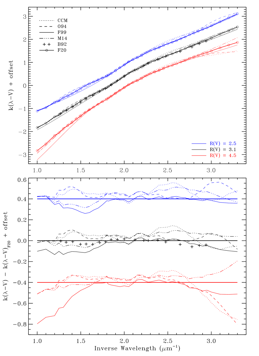
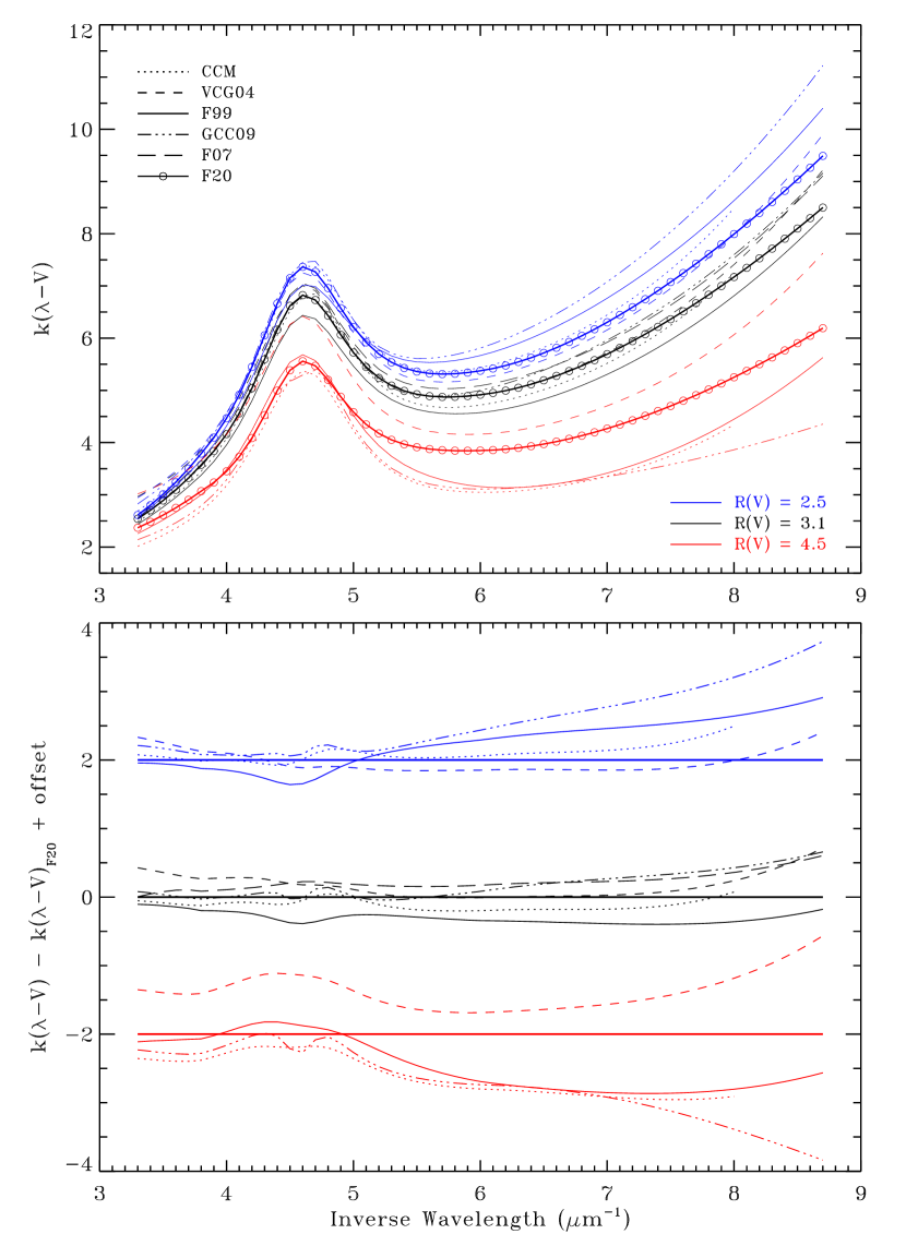
Figure 9: A comparison between our results and previously published estimates of extinction in the optical/NIR (left side) and UV (right side). The extinction curves themselves are shown in the upper half of each panel. The difference between these curves and our new results are shown in the lower half of each panel. Results for several values of $R(V)$ are presented, and identified by different colors (see the lower right portion of each upper panel). The various published studies are distinguished by differing line styles and symbols, as indicated in the top left portion of each upper panel. Vertical offsets are utilized to increase clarity. The key to the various studies, in alphabetical order, is: B92 = Bastiaansen 1992; CCM = Cardelli et al. 1989; F07 = Fitzpatrick & Massa 2007; F20 = this paper; F99 = Fitzpatrick 1999; GCC09 = Gordon et al. 2009; M14 = Maíz Apellániz et al. 2014; O94 = O’Donnell 1994; VCG04 = Valencic et al. 2004.

Our new results are compared with past work in Figure 9. The left and right sides of the figure show the optical/NIR and UV spectral regions, respectively. The top panels on both sides show the extinction curves themselves, while the bottom panels highlight the differences between our results and those of the other investigations. Vertical offsets are used for clarity. Three representative values of $R(V)$ are illustrated (distinguished by color) for most of the comparison studies, which – with the exception of Bastiaansen (1992, “B92”) in the optical and Fitzpatrick & Massa (2007, “F07”) in the UV – all present families of R-dependent curves. B92’s and F07’s results are explicitly measures of mean diffuse medium extinction properties and are grouped with the $R(V)=3.1$ curves. The native units for all the comparison studies are $k(\lambda\!-\!V)$, and so we converted our $k(\lambda\!-\!55)$ curves to $k(\lambda\!-\!V)$ for this comparison, using Equation 4.

In the optical/NIR, the figure shows that the agreement among the various curves is at the level of $\sim$0.1 within and slightly beyond the normalization region (i.e., $\sim$1.6–2.7 $\mu{\rm m}^{-1}$). The work of B92 shows the best agreement with our results (for the case $R(V)=3.1$). B92’s curve was produced using narrowband multi-color photometry, yielding a low-resolution estimate of the true wavelength dependence of the optical curve. The other studies, with the partial exception of Fitzpatrick (1999, “F99”), were not intended to yield detailed representations of the optical extinction law. Rather, they are generally “connect-the-dots” curves guided by the extinction ratios and effective wavelengths from broadband photometry. As such, they only crudely represent the actual shape of the curve, leading to the sizable deviations seen even within the normalization region. In general, these curves do not yield the intended values of $E(B\!-\!V)$, $R(V)$ and other photometric extinction indices when applied to stellar SEDs, as already noted in the previous section for the Calzetti et al. (2000) starburst extinction curve. (See the discussion in F99).

The discrepancies between the comparison curves and ours are larger outside the normalization region. None of the earlier studies utilize measurements in the gap between the optical and UV, and the curves in these regions are extrapolations or interpolations between fundamentally different datasets. Note the large discrepancy in the F99 curve at long wavelengths and large $R(V)$. F99 used a simple interpolation between the optical (at $\sim$6000 Å) and the NIR $JHK$ region and this clearly does not follow the true shape of the curve as revealed by the new spectrophotometry.

The righthand panel of Figure 9 shows good agreement among all the studies on the properties of mean Milky Way extinction in the UV (i.e., for the case $R(V)=3.1$). This is not surprising since there is considerable overlap in the sightlines used in the various studies, all having been drawn from the database of IUE satellite observations. The differences that do exist arise from a number of potential sources, including (1) the specific subset of sightlines used, (2) the use of updated photometry (particularly the 2MASS database), (3) differing techniques used to produce the curves (e.g., pair method vs. extinction-without-standards), and (4) the technique used for deriving the mean curve (e.g., via the $R(V)$-dependence or from a simple average). The differences among the various studies are much larger as $R(V)$ departs from the average Milky Way value. In the most general terms, our results show a weaker overall $R(V)$-dependence than most of the studies illustrated in Figure 9. Given that the $R(V)$-dependences are strongly driven by a relatively small number of sightlines at extreme $R(V)$, the specific sample selections are likely to have a major effect on the results. The other sources of uncertainty listed above for the mean curve are also probable contributors.

To address the sensitivity of our results to the sample selection, we reexamined the 328 star sample from F07. They derived a mean extinction curve from a simple average of all curves with $2.4\leq R(V)\leq 3.6$, but did not quantify the $R(V)$-dependence. We used the same methodology as described in §4.1 to measure the UV $R(V)$-dependence of the 260 stars from F07 for which $\mbox{$E(B\!-\!V)$}>0.30$. The results are shown by the blue dotted curves in the three panels of Figure 6, converted to the $k(\lambda\!-\!55)$ normalization. As can be seen, the F07 sample yielded very similar results to those derived here. Specifically, the $R(55)=3.02$ curve and the sample standard deviation curve are nearly identical to the current results, and virtually indistinguishable in Figure 6 (top and bottom panels), while the $R(V)$-dependence is similar in shape and differs by only $\sim$10% from the current result (middle panel of Figure 6). We conclude that the agreement between F07 and our much smaller current sample indicates that the new results are not subject to a strong sample bias and are generally applicable – at least to the extent that the current body of UV Milky Way extinction measurements can be considered representative of the Milky Way.

5.2 Variations beyond $R$-dependence

Our focus in this paper has been on the trends in the shapes of interstellar extinction curves that can be related to changes in $R$. While this accounts for the broadest trends seen among extinction curves (see Figure 8), it by no means reproduces all the observed sightline-to-sightline variations. The $\sigma[k(\lambda-55)]$ curve in Figure 6 reveals that there is significant scatter around the mean $R$-dependence, which is typically much larger than the individual curve uncertainties (with the likely exception of the longest wavelength G750L observations). This cosmic scatter reveals specific variations among the grain populations that are not distinguished (or distinguishable) by $R$. Notably, the strength of the 2175 Å bump and the level of the curve at the shortest UV wavelengths are only lightly tied to $R$. The level of the far-UV curve is particularly interesting. There are several sightlines (e.g., towards HD 204827, HD 210072, and HD 210121) that are well known for having very steep UV extinction curves, seemingly accompanied by weaker-than-average 2175 Å bumps (see F07). These are not reproduced by our $R$-dependent curves. In fact, these sightlines are among those that were “clipped” from the $R(55)$-dependence because they do not follow the general trend, as can be seen in the bottom panels of Figure 5. These relatively rare, steep far-UV/weak bump sightlines appear to be associated in general with low values of $R$, but not in an easily predictable way. They may represent a separate $R$-dependent sequence of curves or perhaps demonstrate an extreme sensitivity of the curve to grain population details in environments where a generally small value of $R$ pertains. In either case, a detailed study of the grain environments along such sightlines may be necessary to understand the formation of such curves. Extinction studies in external galaxies, such as the Small Magellanic Cloud, where steep/weak-bumped curves appear to be the norm (e.g., Gordon et al., 2003), may also help shed light on the relationship between grain population characteristics and extinction curve properties.

An additional level of curve variability outside the scope of this paper is seen in the fine structure revealed by our measurements of optical extinction. As noted in §3.2 and illustrated in the curves of Figure 4, the optical region contains distinct extinction features known as the Very Broad Structure. A detailed examination of these features is presented by Massa et al. (2020). This study reveals significant sightline-to-sightline variations among these features, which is correlated with other aspects of the extinction curve – but not with $R$. See Massa et al. (2020) for the complete discussion.

6 Summary

We have produced the first spectrophotometrically-derived measurement of the average Milky Way interstellar extinction curve over the wavelength range 1150-to-10000 Å and determined its general dependence on the ratio of total-to-selective extinction in the optical, $R$, over the range $2.5\leq R\leq 6.0$. This curve resolves structures in the optical spectral region down to a level of $\sim$100-200 Å and fully resolves all structure in the UV region.

The curve is based on a unique, homogeneous dataset consisting of IUE and HST/STIS spectrophotometry of normal, early-type stars. These data were all calibrated in a mutually consistent way and fit to model atmospheres to produce a uniform, self-consistent set of extinction curves which span 1150-to-10000 Å at high resolution and extended to 2.2 $\mu{\rm m}$ with broad band $JHK$ photometry. These curves provide the first systematic measurements of extinction in the transition region between past ground-based studies and space-based UV measurements. The use of optical spectrophotometry allowed us to eliminate the uncertainties introduced by normalizing extinction curves by broadband optical photometry and we adopted a monochromatic normalization scheme, based on the extinction at 4400 and 5500 Å. The new curves were used to evaluate the dependence of extinction on $R$ over the full wavelength range and we ultimately parametrized this dependence as a simple linear function of $R$, essentially a first-order Taylor expansion. The Average Milky Way Extinction Curve we present is that which corresponds to the case $R(V)=3.10$. We present this curve in tabular form, along with the linear $R$ dependence and a measure of the curve-to-curve variations about this mean dependence.

Because the coverage between 1150 and 10000 Å is free of gaps and at relatively high resolution, it is possible to use the tabular data to derive the behavior of extinction for any given photometric system, and several examples are presented. The new, high resolution curves also allow the study of extinction features on intermediate wavelength scales in the optical. While such features have been seen before, the new curves show them with considerably more detail and higher signal-to-noise than in the past. The exact shape and sightline-to-sightline variability of this structure is discussed more thoroughly by Massa et al. (2020).

Appendix A STIS Data Reduction

The G430L and G750L spectra are processed with the Instrument Definition Team (IDT) pipeline software written in IDL by D. J. Lindler in 1996–1997. This IDL data reduction is more flexible and offers the following advantages over the STScI pipeline results that are available from the MAST archive:

1. Small shifts in pointing or instrumental flexure between the images of a cosmic ray split (CR-split) observation can often cause an erroneous reduction of net signal, because pixels with the lower signal are retained and the higher pixel value is rejected in the case that the CR-split image pair is not perfectly aligned and pixel pair values differ by more than their statistical noise estimates. Figure 10 shows a standard display of the IDT processing, which makes obvious the deficiency in the reduction with the default of mult_noise=0 parameter for combining the CR-split pair of images that have a small shift. This excess of false CR flags is completely eliminated by a relaxed mult_noise=0.04 value, which does not significantly increase the number of unflagged actual cosmic-ray hits because of our relatively short exposure times. Figure 11 shows the error in extracted spectral signal for mult_noise=0 in black and the corresponding error in the STScI pipeline error of the ocmv0j010_sx1.fits reduction in red. Errors in spectral shape of 2% are common and have two narrower band error features in the STScI standard product. For our observed 98 SNAP program stars, 12 G430L and 7 G750L observations required relaxed values for mult_noise in order to extract the proper spectral signal. For slightly saturated STIS spectral observations, the CR-reject algorithm also fails with a display similar to Figure 10. However, changing mult_noise has little effect. Because saturated data at Gain=4 do not lose charge and the total signal is still present in the raw images, the solution for extracting the proper spectrum is to omit any CR-reject attempts and average the extracted signal from the pair of *flt.fits images. This approach works well in the common case of a bright star and short exposures where cosmic ray hits are minimal.

   

   Figure 10: 1024x1024 pixel STIS CCD image of the G430L CR-split=2 observation of HD146285 (ocmv0j010) on the left and the corresponding image on the right, which flags the location of each falsely detected cosmic ray hit for the default mult_noise=0. Because of a pointing shift between the pair of CR-split images, there is an easily recognized excess of flagged pixels at the location of the spectrum. With a relaxed value of mult_noise=0.04, there is no excess of CR-flagged pixels at the spectral location and the correct combined image of the CR-split pair is produced.

   

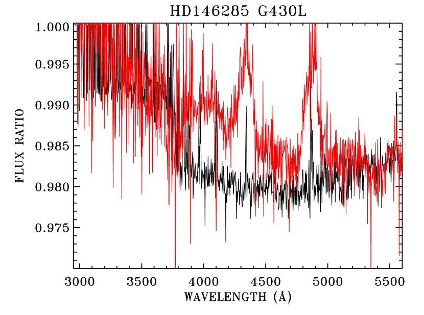
   Figure 11: Ratio (black) of extracted spectra for mult_noise=0 to mult_noise=0.04 for the CR-split=2 observation ocmv0j010 and the ratio (red) of the STScI pipeline reduction ocmv0j010_sx1.fits to the same denominator with the IDL parameter mult_noise=0.04. Errors in spectral shape of up to $\sim$2% exist for the two incorrect spectral extractions.

   

   Figure 12: Fringe flat correction for the G750L spectrum ocmv0j020 of HD146285.

2. For G750L, especially at the longer wavelengths, the spectral width has increased significantly in recent years and a wider extraction height (EXTRSIZE) of 11 pixels, instead of the STScI pipeline EXTRSIZE=7 pixels, is required to maintain photometric repeatability of G750L observations (Bohlin & Proffitt, 2015). The EXTRSIZE=7 spectra show errors in spectral shape of up to 3% in ratio of the long to the short wavelengths of G750L. The wider extraction width encompasses more low signal pixel values, which decreases the spectral S/N slightly.

3. Pixels that are flagged as hot are not used, and those values are reset to the value interpolated in the spectral direction of the affected row of the image before extraction of the spectrum. Very occasionally, a hot pixel flag can occur at the center of a spectral line, resulting in a small reduction in equivalent width. For this paper, our interest is in the continuum and not in precise equivalent width measures.

4. To remove the CCD fringing in G750L, tungsten lamp spectra through the 0.03″x 0.09″slit must be used to align this artificial star with the position of the actual star. The following spline nodes for fitting these tungsten flats are a prerequisite for the G750L sensitivity calibration: 5240, 5265, 5300, 5318, 5340, 5380, 5420, 5460, 5500, 5580, 5700, 5800, 5840, 6000, 6200, 6300, 6450, 6550, 6600, 6620, 6700, 6800, 6900, 7000, 7150, 7400, 7600, 7800, 8000, 8300, 8500, 9100, 9500, 9800, and 10200 Å. These wavelengths are selected to track the features of the tungsten lamp spectrum, while maintaining the proper stiffness and avoiding $\sim$1% bumps due to the $\sim$20% fringe structure at the longer wavelengths. The nodes below 6600 Å are not crucial because the fringe flat is set to unity below 6620 Å. These short-slit tungsten flats are applied to all G750L observations after normalization to unity, reduction of the fringe amplitude by 11% to compensate for narrower PSF of the artificial star, and cross-correlating with the stellar spectrum to remove small residual offsets in the dispersion direction. An example of a fringe flat for ocmv0j020 appears in Figure 12.

In addition to the above data extraction advantages, our post-processing includes the CTE corrections of Goudfrooij et al. (2006) and an up-to-date correction for the changes in STIS sensitivity with time and with temperature. The observations of the three primary flux standards G191B2B, GD153, and GD71, as corrected for CTE and the latest measures of sensitivity change with time, produce a current absolute flux calibration (CALSPEC; see Bohlin et al., 2014).

Appendix B Conversions between extinction relationship equations

Interstellar extinction curves are commonly expressed using the “$k$ ” notation, in the form

$$k(\lambda-V)\equiv\frac{E(\lambda-V)}{E(B-V)}\equiv\frac{A(\lambda)-A(V)}{A(B)-A(V)}\;,$$ (B1)

where $A(\lambda)$ is the total extinction at wavelength $\lambda$ and $B$ and $V$ refer to measurements made using the Johnson $B$ and $V$ filters. A related quantity, commonly known as $R$, is the ratio of total-to-selective extinction in the optical, given by

$$R(V)\equiv\frac{A(V)}{E(B-V)}\;.$$ (B2)

In this paper, we adopt the analogous forms

$$k(\lambda-55)\equiv\frac{E(\lambda-55)}{E(44-55)}\equiv\frac{A(\lambda)-A(55)}{A(44)-A(55)}\;,$$ (B3)

and

$$R(55)\equiv\frac{A(55)}{E(44-55)}\;,$$ (B4)

in which measurements with the Johnson $B$ and $V$ filters are replaced by monochromatic measurements at 4400 and 5500 Å, respectively. Our data show that the two normalizations are related by

$$k(\lambda-55)=\alpha\;k(\lambda-V)+\beta\;,$$ (B5)

which implies

$$R(55)=\alpha\;R(V)-\beta\;.$$ (B6)

The precise values of $\alpha$ and $\beta$ depend on the shapes of the stellar energy distributions (reddened and unreddened), due to the broadband nature of the $B$ and $V$ filters. For our particular sample, which on average consists of middle B stars with $E(B-V)\simeq 0.5$, we find that $\alpha=0.990$ and $\beta=0.049$. With these coefficients, the generally accepted Milky Way mean value of $R(V)_{0}=3.10$ corresponds to $R(55)_{0}=3.02$.

As described in the text, we find the following functional relationship between the $k(\lambda-55)$ extinction curves and $R(55)$

$$k(\lambda-55)=s(\lambda-55)\;[R(55)-R(55)_{0}]+k(\lambda-55)_{0}\;,$$ (B7)

which is essentially a first order Taylor expansion in $R(55)$ at each wavelength. In this equation, $s(\lambda-55)$ is the observed slope between $R(55)$ and $k(\lambda-55)$, $R(55)_{0}$ is the average Milky Way value of $R(55)$, and $k(\lambda-55)_{0}$ is the extinction curve corresponding to $R(55)_{0}$. The complete set of $k(\lambda-55)_{0}$ and $s(\lambda-55)$ values, which allow a detailed extinction curve to be constructed over the range 1150 to 10000 Å, are given in Table 3.

In their early investigation of the $R$-dependence of extinction, CCM adopted a different extinction curve normalization, i.e., $A(\lambda)/A(V)$. From Equations B1 and B2, it can be seen that this is related to $k(\lambda-V)$ by

$$\frac{A(\lambda)}{A(V)}=\frac{k(\lambda-V)}{R(V)}+1\>.$$ (B8)

CCM parameterized the $R$-dependence of $A(\lambda)/A(V)$ as

$$\frac{A(\lambda)}{A(V)}=a(\lambda)+b(\lambda)R(V)^{-1}\>.$$ (B9)

At first look, this appears to be a very different functional relationship between $R$ and the shape of the extinction curve than we have found (i.e., Eq. B7). However, when Equation B8 is substituted into Equation B9, the following result is obtained:

$$k(\lambda-V)=[a(\lambda)-1]R(V)+b(\lambda)\>.$$ (B10)

Thus it is seen that, like us, CCM found their extinction curves to be linearly related to $R$, when expressed in the “$k$ ” notation. Moreover, the relationship between CCM’s $a(\lambda)$ and $b(\lambda)$ and our coefficients $s(\lambda-55)$ and $k(\lambda-55)_{0}$ can be found by comparing Equations B7 and B10 and making the appropriate substitutions from Equations B5 and B6. The result is

$$a(\lambda) = s(\lambda-55)+1$$

$$b(\lambda) = -s(\lambda-55)\left[\frac{R(55)_{0}+\beta}{\alpha}\right]+\left[\frac{k(\lambda-55)_{0}-\beta}{\alpha}\right]\>.$$ (B11)

In principal, identical results would be achieved regardless of whether our “$k$” normalization or CCM’s $A(\lambda)$ normalization were used. One must keep in mind, however, that these mathematical transformations only apply in the absense of errors. Least squares solutions resulting from the two different formulations could yield different results.

References

- Aiello et al. (1988) Aiello, S., Barsella, B., Chlewicki, G., et al. 1988, Astronomy and Astrophysics Supplement Series, 73, 195
- Aiello et al. (1982) Aiello, S., Barsella, B., Guidi, I., Penco, U., & Perinotto, M. 1982, Ap&SS, 87, 463
- Bastiaansen (1992) Bastiaansen, P. A. 1992, A&AS, 93, 449
- Boggs & Bohm-Vitense (1989) Boggs, D., & Bohm-Vitense, E. 1989, ApJ, 339, 209
- Bohlin et al. (2014) Bohlin, R. C., Gordon, K. D., & Tremblay, P. E. 2014, PASP, 126, 711
- Bohlin et al. (2017) Bohlin, R. C., Mészáros, S., Fleming, S. W., et al. 2017, AJ, 153, 234
- Bohlin & Proffitt (2015) Bohlin, R. C., & Proffitt, C. R. 2015, Instrument Science Report STIS 2015-01 (v1), 20 pages, 1
- Borgman (1960) Borgman, J. 1960, Bulletin of the Astronomical Institutes of the Netherlands, 15, 255
- Bostroem & Proffitt (2011) Bostroem, K. A., & Proffitt, C. 2011, STIS Data Handbook v. 6.0
- Bouigue (1959) Bouigue, M. R. 1959, Publications of the Observatoire Haute-Provence, 4, 52
- Boulon et al. (1958) Boulon, J., Duflot, M., & Fehrenbach, C. 1958, Journal des Observateurs, 42, 1
- Calzetti et al. (2000) Calzetti, D., Armus, L., Bohlin, R. C., et al. 2000, ApJ, 533, 682
- Calzetti et al. (1994) Calzetti, D., Kinney, A. L., & Storchi-Bergmann, T. 1994, ApJ, 429, 582
- Cardelli et al. (1989) Cardelli, J. A., Clayton, G. C., & Mathis, J. S. 1989, ApJ, 345, 245
- Casagrande & VandenBerg (2014) Casagrande, L., & VandenBerg, D. A. 2014, MNRAS, 444, 392
- Clayton & Fitzpatrick (1987) Clayton, G. C., & Fitzpatrick, E. L. 1987, AJ, 93, 157
- Clayton et al. (2000) Clayton, G. C., Gordon, K. D., & Wolff, M. J. 2000, ApJS, 129, 147
- Clayton et al. (2003) Clayton, G. C., Wolff, M. J., Sofia, U. J., Gordon, K. D., & Misselt, K. A. 2003, ApJ, 588, 871
- Cohen et al. (1992) Cohen, M., Walker, R. G., Barlow, M. J., & Deacon, J. R. 1992, AJ, 104, 1650
- Cohen et al. (2003) Cohen, M., Wheaton, W. A., & Megeath, S. T. 2003, AJ, 126, 1090
- Cowley et al. (1969) Cowley, A., Cowley, C., Jaschek, M., & Jaschek, C. 1969, AJ, 74, 375
- Crawford (1975) Crawford, D. L. 1975, PASP, 87, 481
- Divan (1954) Divan, L. 1954, Annales d’Astrophysique, 17, 456
- Doi et al. (2010) Doi, M., Tanaka, M., Fukugita, M., et al. 2010, AJ, 139, 1628
- Domínguez et al. (2013) Domínguez, A., Siana, B., Henry, A. L., et al. 2013, ApJ, 763, 145
- Feast et al. (1955) Feast, M. W., Thackeray, A. D., & Wesselink, A. J. 1955, Memoirs of the Royal Astronomical Society, 67, 51
- Feast et al. (1957) —. 1957, Memoirs of the Royal Astronomical Society, 68, 1
- Fitzgerald (1970) Fitzgerald, M. P. 1970, A&A, 4, 234
- Fitzpatrick (1999) Fitzpatrick, E. L. 1999, PASP, 111, 63
- Fitzpatrick (2004) Fitzpatrick, E. L. 2004, in Astronomical Society of the Pacific Conference Series, Vol. 309, Astrophysics of Dust, ed. A. N. Witt, G. C. Clayton, & B. T. Draine, 33
- Fitzpatrick & Massa (1986) Fitzpatrick, E. L., & Massa, D. 1986, ApJ, 307, 286
- Fitzpatrick & Massa (1988) —. 1988, ApJ, 328, 734
- Fitzpatrick & Massa (1990) —. 1990, ApJS, 72, 163
- Fitzpatrick & Massa (2005a) —. 2005a, AJ, 130, 1127
- Fitzpatrick & Massa (2005b) —. 2005b, AJ, 129, 1642
- Fitzpatrick & Massa (2007) —. 2007, ApJ, 663, 320
- Gallagher et al. (1984) Gallagher, III, J. S., Hunter, D. A., & Tutukov, A. V. 1984, ApJ, 284, 544
- Garrison (1967) Garrison, R. F. 1967, ApJ, 147, 1003
- Garrison & Kormendy (1976) Garrison, R. F., & Kormendy, J. 1976, Publications of the Astronomical Society of the Pacific, 88, 865
- Gordon et al. (2009) Gordon, K. D., Cartledge, S., & Clayton, G. C. 2009, ApJ, 705, 1320
- Gordon et al. (2003) Gordon, K. D., Clayton, G. C., Misselt, K. A., Land olt, A. U., & Wolff, M. J. 2003, ApJ, 594, 279
- Goudfrooij et al. (2006) Goudfrooij, P., Maíz Apellániz, J., Brown, T., & Kimble, R. 2006, Charge Transfer Efficiency of the STIS CCD:The time dependence of charge loss and centroid shiftsfrom Internal Sparse Field data, Tech. rep.
- Gray & Corbally (1994) Gray, R. O., & Corbally, C. J. 1994, AJ, 107, 742
- Grevesse et al. (2013) Grevesse, N., Asplund, M., Sauval, A. J., & Scott, P. 2013, in Astronomical Society of the Pacific Conference Series, Vol. 479, Progress in Physics of the Sun and Stars: A New Era in Helio- and Asteroseismology, ed. H. Shibahashi & A. E. Lynas-Gray, 481
- Grevesse & Sauval (1998) Grevesse, N., & Sauval, A. J. 1998, Space Sci. Rev., 85, 161
- Guetter (1968) Guetter, H. H. 1968, Publications of the Astronomical Society of the Pacific, 80, 197
- Hackwell et al. (1991) Hackwell, J. A., Hecht, J. H., & Tapia, M. 1991, ApJ, 375, 163
- Herbig (1975) Herbig, G. H. 1975, ApJ, 196, 129
- Hill (1970) Hill, P. W. 1970, MNRAS, 150, 23
- Hiltner (1956) Hiltner, W. A. 1956, The Astrophysical Journal Supplement Series, 2, 389
- Hoffleit (1956) Hoffleit, D. 1956, ApJ, 124, 61
- Houk (1978) Houk, N. 1978, Michigan catalogue of two-dimensional spectral types for the HD stars
- Houk & Cowley (1975) Houk, N., & Cowley, A. P. 1975, University of Michigan Catalogue of two-dimensional spectral types for the HD stars. Volume I. Declinations -90 to -53
- Johnson (1962) Johnson, H. L. 1962, ApJ, 136, 1135
- Johnson & Borgman (1963) Johnson, H. L., & Borgman, J. 1963, Bulletin of the Astronomical Institutes of the Netherlands, 17, 115
- Johnson & Morgan (1953) Johnson, H. L., & Morgan, W. W. 1953, ApJ, 117, 313
- Johnson & Morgan (1955) —. 1955, ApJ, 122, 429
- Kennicutt (1983) Kennicutt, Jr., R. C. 1983, ApJ, 272, 54
- Kurucz (1991) Kurucz, R. L. 1991, in NATO Advanced Science Institutes (ASI) Series C, Vol. 341, NATO Advanced Science Institutes (ASI) Series C, ed. L. Crivellari, I. Hubeny, & D. G. Hummer, 441
- Lanz & Hubeny (2003) Lanz, T., & Hubeny, I. 2003, ApJS, 146, 417
- Lanz & Hubeny (2007) —. 2007, ApJS, 169, 83
- Maíz Apellániz (2007) Maíz Apellániz, J. 2007, in Astronomical Society of the Pacific Conference Series, Vol. 364, The Future of Photometric, Spectrophotometric and Polarimetric Standardization, ed. C. Sterken, 227
- Maíz Apellániz & Pantaleoni González (2018) Maíz Apellániz, J., & Pantaleoni González, M. 2018, A&A, 616, L7
- Maíz-Apellániz et al. (2004) Maíz-Apellániz, J., Walborn, N. R., Galué, H. Á., & Wei, L. H. 2004, The Astrophysical Journal Supplement Series, 151, 103
- Maíz Apellániz et al. (2014) Maíz Apellániz, J., Evans, C. J., Barbá, R. H., et al. 2014, A&A, 564, A63
- Massa & Fitzpatrick (2000) Massa, D., & Fitzpatrick, E. L. 2000, ApJS, 126, 517
- Massa et al. (2020) Massa, D., Fitzpatrick, E. L., & Gordon, K. D. 2020, ApJ, submitted
- Massa et al. (1983) Massa, D., Savage, B. D., & Fitzpatrick, E. L. 1983, ApJ, 266, 662
- Massey & Johnson (1993) Massey, P., & Johnson, J. 1993, AJ, 105, 980
- Mathis & Cardelli (1992) Mathis, J. S., & Cardelli, J. A. 1992, ApJ, 398, 610
- Meadows (1961) Meadows, A. J. 1961, MNRAS, 123, 81
- Metreveli (1968) Metreveli, M. D. 1968, Abastumanskaia Astrofizicheskaia Observatoriia Byulleten, 38, 93
- Morgan et al. (1978) Morgan, W. W., Abt, H. A., & Tapscott, J. W. 1978, Revised MK Spectral Atlas for stars earlier than the sun
- Morgan et al. (1955) Morgan, W. W., Code, A. D., & Whitford, A. E. 1955, The Astrophysical Journal Supplement Series, 2, 41
- Morgan et al. (1953) Morgan, W. W., Whitford, A. E., & Code, A. D. 1953, ApJ, 118, 318
- Morrell et al. (1988) Morrell, N., Garcia, B., & Levato, H. 1988, Publications of the Astronomical Society of the Pacific, 100, 1431
- Muzzio & Rydgren (1974) Muzzio, J. C., & Rydgren, A. E. 1974, AJ, 79, 864
- O’Donnell (1994) O’Donnell, J. E. 1994, ApJ, 422, 158
- Osawa (1959) Osawa, K. 1959, ApJ, 130, 159
- Panek (1983) Panek, R. J. 1983, ApJ, 270, 169
- Racine (1968a) Racine, R. 1968a, AJ, 73, 588
- Racine (1968b) —. 1968b, AJ, 73, 233
- Riley et al. (2019) Riley, A., et al. 2019, STIS Instrument Handbook v. 18.0
- Roman (1955) Roman, N. G. 1955, The Astrophysical Journal Supplement Series, 2, 195
- Schild et al. (1971) Schild, R., Neugebauer, G., & Westphal, J. A. 1971, AJ, 76, 237
- Schild (1965) Schild, R. E. 1965, ApJ, 142, 979
- Schild & Chaffee (1971) Schild, R. E., & Chaffee, F. 1971, ApJ, 169, 529
- Slettebak (1968) Slettebak, A. 1968, ApJ, 154, 933
- Smartt et al. (1996) Smartt, S. J., Dufton, P. L., & Rolleston, W. R. J. 1996, A&A, 305, 164
- Smith (1972) Smith, M. A. 1972, ApJ, 175, 765
- Turner et al. (1980) Turner, D. G., Grieve, G. R., Herbst, W., & Harris, W. E. 1980, AJ, 85, 1193
- Valencic et al. (2004) Valencic, L. A., Clayton, G. C., & Gordon, K. D. 2004, ApJ, 616, 912
- van Leeuwen (2007) van Leeuwen, F. 2007, A&A, 474, 653
- Vrba & Rydgren (1984) Vrba, F. J., & Rydgren, A. E. 1984, ApJ, 283, 123
- Walborn (1971) Walborn, N. R. 1971, ApJS, 23, 257
- Weingartner & Draine (2001) Weingartner, J. C., & Draine, B. T. 2001, ApJ, 548, 296
- Whiteoak (1966) Whiteoak, J. B. 1966, ApJ, 144, 305
- Whitford (1958) Whitford, A. E. 1958, AJ, 63, 201
- Witt et al. (1984) Witt, A. N., Bohlin, R. C., & Stecher, T. P. 1984, ApJ, 279, 698
- York (1971) York, D. G. 1971, ApJ, 166, 65
- Zubko et al. (2004) Zubko, V., Dwek, E., & Arendt, R. G. 2004, ApJS, 152, 211