Atmospheric Neutrinos

Abstract

Atmospheric neutrinos produced by cosmic-ray interactions around the globe provide a beam for the study of neutrino properties. They are also a background in searches for neutrinos of astrophysical origin. Both aspects are addressed in this chapter, which begins with a brief introduction on neutrino oscillations in relation to the spectrum of atmospheric neutrinos. Section 2 describes the cascade equation for hadrons in the atmosphere and the main features of atmospheric leptons from their decays. Next, uncertainties in the fluxes that arise from limited knowledge of the primary spectrum and of particle production are discussed. The final section covers aspects specific to neutrino telescopes.

0.1 Introduction

The discovery of atmospheric neutrino oscillations was announced twenty years ago by Super-Kamiokande [1]. The key observation was the energy-dependence of the ratio of electron to muon neutrinos, comparing fluxes from below the horizon with those from above. Simple counting of the low-energy decay chains leads to the expectation of two muon neutrinos for every electron neutrino. The observed ratio was closer to one for sub-GeV neutrinos and remained low into the GeV region for those from below with pathlengths of $\sim 10^{4}$ km, while the ratio increased for the neutrinos produced above the detector at the typical altitude of $15$ km. The interpretation was that muon neutrinos and tau neutrinos mix and can oscillate between each other, and the low-energy $\nu_{\tau}$ were below detection threshold.

Interpretation of the measurements was based on calculations of the flux of atmospheric muon- and electron-neutrinos that existed at the time [2, 3] and [4, 5] in which secondary neutrinos were assumed to be in the same direction as the parent cosmic-rays from which they descended. The importance of making three-dimensional calculations for low-energy neutrinos was emphasized by Battistoni et al. [6]. There followed other three-dimensional calculations that also accounted for the significant effects of the geomagnetic field at Kamioka, as well as for solar modulation, for example [7, 8]. The flux of atmospheric neutrinos in the context of oscillations was reviewed at the time in Ref. [9], including the important azimuth angular dependence (“East-West effect") that results from the high geomagnetic cutoffs in Japan. Effects of solar modulation were also discussed, and the primary spectrum used for the calculations was described.

Measurements of atmospheric neutrinos at Soudan [10] and MACRO [11] confirmed the Super-K results. To a good first approximation, the atmospheric neutrinos are interpreted in a two flavor scenario characterized by $\theta_{23}\approx\frac{\pi}{4}$ and $\delta m^{2}_{23}\approx 2.5\times 10^{-3}$ eV². Reference [12] reports the fluxes of atmospheric neutrinos after oscillations and averaged over directions as observed in the four phases of Super-K operation. The strong azimuthal effect is studied in detail and well understood in terms of geomagnetic effects on the incident cosmic rays. The effect of solar modulation is more difficult to see at Super-K because of the relatively high geomagnetic cutoff. Oscillations of atmospheric neutrinos measured by IceCube [13] in the energy range 6 to 56 GeV show consistency with long-baseline results at lower $E_{\nu}$.

Measurement of both charged current and neutral current interactions of solar neutrinos by SNO [14] determined that the solar neutrino problem was the result of oscillations involving electron neutrinos, characterized by parameters $\theta_{12}\approx 33^{\circ}$ and $\delta m^{2}_{12}\approx 7.5\times 10^{-5}$eV². Additional measurements by Daya Bay [15], RENO [16] and Double Chooz [17] reactors using electron anti-neutrinos from reactors determined $\theta_{13}$, the third link in the three-flavor oscillation framework. Long baseline measurements, KamLAND [18], MINOS [19] and T2K [20], coupled with reactor experiments provide further refinement of the oscillation parameters. Reference [21] is the three-flavor analysis of the Super-K data. For a full review of neutrino oscillations see the PDG article [22, 23].

An important implication of atmospheric oscillations is that there must be a substantial flux of atmospheric $\tau$-neutrinos transformed via oscillations from muon neutrinos. These are, however, not easy to measure because of the small cross section in the threshold region to produce the $\tau$-lepton with mass $\approx 1.9$ m_p. Measurements at Super-K [24] with atmospheric neutrinos and at OPERA [25] at Gran Sasso in the beam from CERN are consistent with expectation. An effort to measure $\nu_{\tau}$ appearance with neutrinos in IceCube DeepCore is underway [26]. One goal is to check for unitarity of the three-flavor mixing matrix. A deficit of $\tau$-neutrinos could be a signal for sterile neutrinos. Other possible signals of physics beyond the standard model discussed in this volume include non-standard neutrino interactions and violation of Lorentz invariance. For all such searches, a good knowledge of the atmospheric neutrino spectrum is essential.

The main implication for neutrino astronomy is that neutrinos from distant sources should contain $\tau$-neutrinos at comparable levels to the other two flavors [27].

0.2 Phenomenology of neutrino spectra

The atmospheric cascade is initiated by primary cosmic rays interacting with nuclei in the atmosphere. Since production of mesons occurs at the level of nucleon-nucleon interactions, calculation of the inclusive spectra of atmospheric leptons starts from the spectrum of nucleons as a function of energy per nucleon. In the superposition approximation, the points of first interaction of the nucleons from a primary cosmic-ray of mass number $A$ are distributed on average as if each of its nucleons were injected independently and interacted with an interaction length in g/cm² of

$$\lambda_{N}=A_{\rm air}\,m_{p}\,/\,\sigma_{p-air}^{\rm inel}$$ (1)

The cascade equation for hadrons in the atmosphere is then

$$\frac{{\rm d}N_{i}(E_{i},X)}{{\rm d}X} = -\frac{N_{i}(E_{i},X)}{\lambda_{i}}-\frac{N_{i}(E_{i},X)}{d_{i}}$$

$$+\sum_{j=i}^{J}\int_{E}^{\infty}\,\frac{F_{ji}(E_{i},E_{j})}{E_{i}}\,\frac{N_{j}(E_{j},X)}{\lambda_{j}}\,{\rm d}E_{j}.$$

The variable $X$ is the slant depth in g/cm² of atmosphere along the direction of the primary cosmic-ray, and $N_{i}(E_{i},X)$ is the number of particles of type $i$ at that slant depth. Interaction lengths $\lambda_{i}$ for each type of hadron are defined in analogy to the interaction length for nucleons in Eq. 1. The first term on the right-hand side of Eq. 0.2 is loss due to interactions in the atmosphere, while the second represents loss by decay. For consistency, the decay length has to be expressed in g/cm², so

$$d_{i}(X)=\rho(X)\,\gamma\,c\,\tau_{i},$$ (3)

for a particle with rest lifetime $\tau_{i}$ and Lorentz factor $\gamma$ at a slant-depth $X$ where the density of the atmosphere is $\rho(X)$.

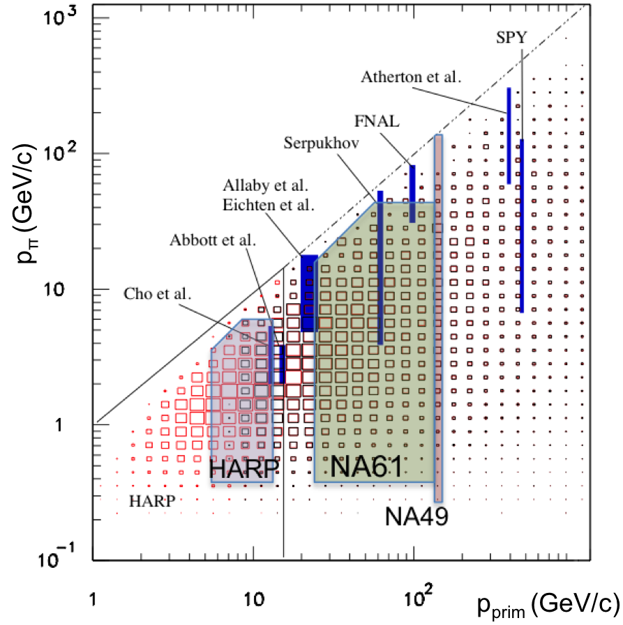
Figure 1: Phase space diagram for the calculation [8] of contained neutrinos at Super-K. (Figure updated from Ref. [28], see text for explanation.)

The last term in Eq. 0.2 accounts for production of particles of type $i$ by particles of type $j$ and energy $E_{j}>E_{i}$. Its definition is

$$F_{ji}(E_{i},E_{j})\equiv E_{i}\frac{1}{\sigma^{\rm air}_{j}}\frac{{\rm d}\sigma_{j\,{\rm air}\rightarrow i}}{{\rm d}E_{i}}=E_{i}\frac{{\rm d}n_{ji}(E_{i},E_{j})}{{\rm d}E_{i}},$$ (4)

where d$n_{i}$ is the number of particles of type $i$ produced on average in the energy bin d$E_{i}$ around $E_{i}$ per collision of an incident particle of type $j$. Defined in this way, $F_{ji}$ is a dimensionless quantity. This definition is motivated by the fact that cross sections vary slowly with energy and the inclusive cross sections at high energy exhibit an approximate scaling behavior such that $F(E_{i},E_{j})\approx F(x_{L})$, where $x_{L}=E_{i}/E_{j}$ is the ratio of lab energies. Spectrum-weighted moments of $F(x_{L})$ defined as

$$Z_{ji}\equiv\int_{0}^{1}\,(x_{L})^{\gamma-1}\,F_{ji}(x_{L})\;{\rm d}x_{L}\,=\,\int_{0}^{1}(x_{L})^{\gamma}\frac{{\rm d}n_{ji}}{{\rm d}x_{L}}{\rm d}x_{L}$$ (5)

appear in the approximate solutions to Eq. 0.2 to be discussed below, in which the spectrum of nucleons is approximated as a power law with an integral index $\gamma$.

The blue bars in Figure 1 from Ref. [28] show the phase space covered by experiments used for the calculation of Ref. [8]. More recent data sets from HARP [29], NA49 [30, 31] and NA61/SHINE [32, 33] are also indicated. The underlying 2-D histogram shows the distribution of the primary cosmic-ray nucleon and parent pion energies for neutrinos in the energy region of contained event sample of Super-K from the simulation of Ref. [8]. The red area below $8$ GeV is excluded by the geomagnetic cutoff at Super-K. Each row in the histogram is the integrand of $Z_{p\pi}$ from Eq. 5 weighted by the efficiency for “contained" events. The integrand of the Z-factor is proportional to the product of the spectrum of nucleons and the yield of charged pions. The distribution for a higher-energy event sample would be shifted to higher energy, but would display the same qualitative features of a rise of intensity at threshold and decrease at high energy reflecting the steepness of the primary spectrum. These factors are illustrated below in Fig. 10. Estimates of uncertainties in the meson yields in Ref.[28] need to be updated to include the more recent data sets and to extend the uncertainty estimates to higher energy.

For unstable mesons the competition between decay and interaction is determined by Eq. 3 compared to the interaction length. The pressure at vertical depth $X_{v}$ is determined by the weight of the column of air above; $P=gX_{v}\approx gX\cos\theta$, where the flat Earth approximation for slant depth is good for zenith angle $\theta<70^{\circ}$. Using the ideal gas law to relate density, pressure and temperature leads to the relation

$$\frac{1}{d_{i}}=\frac{\epsilon_{i}}{EX\cos\theta}\,\,{\rm with}\,\epsilon_{i}=\frac{m_{i}c^{2}}{c\tau_{i}}\frac{RT}{gM},$$ (6)

with $M=0.02896$ kg/mol for air. The quantity $RT\,/\,gM$ has the dimension of length. It is the local scale height at $X_{v}$ of an exponential approximation to the atmospheric density as a function of altitude: $X_{v}\approx X_{0}\exp\{-h/h_{0}\}$ with $h_{0}\approx 6.5$ km for a temperature of $220^{\circ}$K and $X_{0}\approx 1030$ g/cm² at sea level. For example, when $E_{\pi}\approx\epsilon_{\pi}$ the decay and interaction terms in Eq. 0.2 are comparable when $X_{v}=\lambda_{N}\approx 85$ g/cm², which corresponds to an altitude of about $15$ km, the typical production height of most muons.

For $E_{i}<<\epsilon_{i}$ the parent mesons decay before interacting and the lepton spectrum directly reflects the primary spectrum of nucleons. As energy increases ($E_{i}>\epsilon_{i}$), decay becomes increasingly unlikely relative to re-interaction of the mesons. In the high-energy limit, the meson fluxes reflect the primary spectrum, and their probability of decay is proportional to the decay probability. For example, the spectrum of decaying pions is

$${\cal D}_{\pi}(E,X)\,=\,\frac{1}{d_{\pi}}\Pi(E,X)\,=\,\frac{\epsilon_{\pi}\sec\theta}{EX}\Pi(E,X),$$ (7)

where $\Pi(E,X)$ is the solution of Eq. 0.2 for pions in the high-energy limit. Thus the spectrum of atmospheric leptons at high energy is asymptotically one power steeper than the parent hadron spectra. The $\sec\theta$ factor in Eq. 7 implies that the transition to the steeper energy spectrum occurs at higher energy for large zenith angles. As a consequence, for a given $E>\epsilon$, the intensity of leptons increases with increasing zenith angle.

It is worth noting that the basic features of the spectrum of atmospheric neutrinos were explained by Zatsepin and Kuz’min [34] in 1961, including the important role of kaons relative to pions as parents of neutrinos. Their papers include the production of neutrinos from decay of muons, and they describe the strong angular dependence at high energy, which is a consequence of the $\sec\theta$ dependence of the ratio of decay to interaction above the critical energies of the mesons. They also explain that charged kaons are more efficient producers of neutrinos than charged pions because of the higher mass of the kaon relative to the muon and the shorter lifetime of the kaon. (See the discussion of Eq. 8 below.) In the 60’s and 70’s Volkova and Zatsepin published a series of papers refining the early calculations, as described in the paper of Volkova [35], which remains a standard reference for fluxes of atmospheric neutrinos.

0.2.1 Solving the cascade equations

The most general approach to solving the cascade equations is a full Monte Carlo. This method is necessary for atmospheric neutrinos at low energy where three-dimensional effects must be accounted for. It is also the standard approach for air showers. Each event generated is an instance of a solution of the cascades equations subject to a $\delta$-function boundary condition, namely $N_{A}(E,X=0)=\delta(E-E_{A})$ for the primary nucleus of mass $A$ and zero for all other species. Simulated events need to be re-weighted to match a specific primary spectrum and composition. However, a full Monte Carlo becomes inefficient for atmospheric leptons of high energy because the decay probability of the parent mesons decreases with energy according to Eq. 6. Biased Monte Carlos may be designed to increase the efficiency for special purposes by rejecting events as soon as it can be ascertained that they will not be included in the desired class of events. A recent example is the generalized atmospheric-neutrino self-veto [36] where specialized simulations [37] are used to verify the calculation.

For the calculation of atmospheric muons and neutrinos above a few GeV, linear solutions of the cascade equations are sufficient. In this case, a classic approach is to integrate the equations numerically step by step through the atmosphere. The most advanced and modern version of this approach is the Matrix Cascade Equation (MCEq) solver [38, 39]. MCEq has been used recently [40] to obtain fluxes of atmospheric muons and neutrinos from Sibyll 2.3c [41]. An advantage of MCEq is that all relevant hadronic species are followed so that relatively small contributions to the fluxes can be assessed, including, for example, the contribution of the decay of unflavored mesons to prompt muons. In addition, the solver handles the integration along trajectories near the horizon correctly.

To demonstrate the basic features of the energy- and angular-dependence of atmospheric neutrinos, approximate analytic solutions of Eq. 0.2 in which only the main contributing mesons are included are instructive. Three simplifying assumptions lead to the solutions:

1. a power-law in energy for the differential spectrum of primary nucleons
   $\phi_{N}(E_{N})\propto E_{N}^{-(\gamma+1)}$,

2. scaling for the inclusive production cross sections
   $F_{ij}(E_{i},E_{j})=F_{ij}(E_{i}/E_{j})$, and

3. constant interaction and production cross sections.

The boundary condition for inclusive fluxes is $N_{i}(E,X=0)=\phi_{N}(E_{N})$, where $\phi_{N}$ is the differential flux of nucleons, and zero for all other hadrons.

Analytic solutions are obtained for the production spectrum of leptons as a function of slant depth $X$ in two energy regions, $E\cos\theta$ much less than and much greater than the relevant critical energies. For example, for $E_{\pi}\cos\theta>>\epsilon_{\pi}$ the production spectra of $\nu_{\mu}$ and $\mu$ are obtained from Eq. 7 by multiplying by the decay distribution for $\pi^{\pm}\rightarrow\mu+\nu_{\mu}$ and integrating over the parent pion energies allowed for a given lepton energy. In the center of mass system, the momenta of the neutrino and the muon are equal and opposite, but because of the large mass of the muon compared to that of the neutrino, the two distributions are significantly different when transformed to the lab system. The multiplicative decay factors at high energy are

$$Z_{\pi\mu}=\frac{(1-r_{\pi}^{\gamma+2})}{(\gamma+2)(1-r_{\pi})}\,\,\,\,{\rm and}\,\,\,Z_{\pi\nu_{\mu}}=\frac{(1-r_{\pi})^{\gamma+2}}{(\gamma+2)(1-r_{\pi})},$$ (8)

where $r_{\pi}=\frac{m_{\mu}^{2}}{m_{\pi}^{2}}=0.573$ and $\gamma\approx 1.7$ is the integral spectral index. Numerically, these factors are quite different for $\nu_{\mu}$ and $\mu$. The differences are much less for the channel $K^{\pm}\rightarrow\mu+\nu_{\mu}$ because $r_{K}\approx 0.046$ is small.

Full details of the derivation of the analytic approximations are given in Chapter 6 of Ref. [42]. Integrating over the production spectra and combining the high- and low-energy expressions with an interpolation formula leads to the following expression for the muon neutrino spectrum ($\nu+\overline{\nu}$):

$$\frac{{\rm d}N_{\nu}}{{\rm d}E_{\nu}} \simeq \frac{N_{0}(E_{\nu})}{1-Z_{NN}}\left\{\frac{{\cal A}_{\pi\nu}}{1+{\cal B}_{\pi\nu}\cos{\theta}\,E_{\nu}/\epsilon_{\pi}}\right.$$

$$\left.+\;0.635\frac{\,{\cal A}_{K\nu}}{1+{\cal B}_{K\nu}\cos{\theta}\,E_{\nu}/\epsilon_{K}}\,+\,\sum_{i}B_{D_{i}}\frac{{\cal A}_{D\nu}}{1+{\cal B}_{D\nu}\cos{\theta}\,E_{\nu}/\epsilon_{D}}\right\}.$$

The scaling assumption, in combination with the power-law form for the primary spectrum, allows the neutrino spectrum to be expressed as a product of the spectrum of primary nucleons evaluated at the energy of the lepton and a sum of contributions from pion decay, from kaon decay and from decay of charmed hadrons. The factor $1/(1-Z_{NN})$ accounts for the regeneration of nucleons in the cascade. The contribution from muon decay, which becomes important at low energy, is not included here.

The equation for $\mu^{+}+\mu^{-}$ has the same form but with different decay factors as in Eq. 8. In addition, there is a multiplicative factor to account for survival probability against energy loss and decay. The losses are negligible in the TeV range and above, but become increasingly significant at lower energies and for large zenith angles.

Table 1: Critical energies, $\epsilon_{i}$ (GeV)

$\mu$	$\pi^{\pm}$	K±	D±	D0
1.	115.	850.	3.9$\times 10^{7}$	9.9$\times 10^{7}$

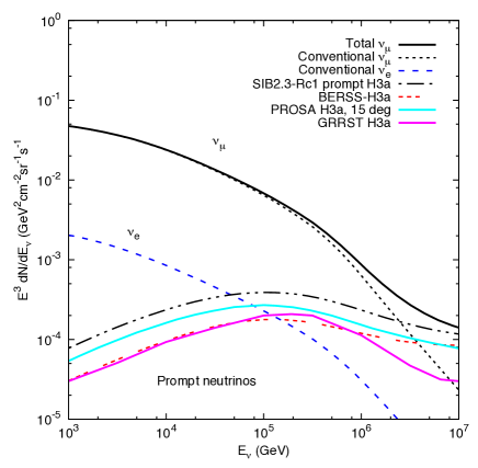
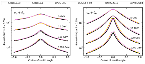
Figure 2: Fluxes of neutrinos ($\nu_{\mu}+\overline{\nu}_{\mu}$) with the contribution from charm shown separately for four models [43, 44, 45, 46]. The flux of electron neutrinos is calculated in Ref. [47]

Figure 3: Zenith angle distributions from Ref.[40] for $\nu_{\mu}+\overline{\nu}_{\mu}$ (left) and $\nu_{e}+\overline{\nu}_{e}$ (right) normalized to 1 at $\cos\theta=0.55$. The lower energy curves are raised by successive factors of five.

The basic structure is the same for each term in Eq. 0.2.1, but they contribute differently in different regions of energy and angle because of their different critical energies (see Table 1). For $E_{\nu}\cos\theta<<\epsilon_{i}$ the contribution to the neutrino flux is isotropic and has the same spectral index as the primary cosmic rays (a differential spectral index $\approx 2.7$ below the knee). For $E_{\nu}\cos\theta>>\epsilon_{i}$ each contribution to the neutrino flux is proportional to $\sec\theta$ and has a spectral index one power steeper than the primary spectrum. At each zenith angle there is a gradual steepening of the energy spectrum, which occurs at significantly higher energy near the horizontal. Figure 3 shows the conventional neutrino spectra averaged over zenith angle and Fig. 3 from Ref.[40] shows the shapes of the distributions as a function of zenith angle. The composite energy spectrum steepens gradually, at first because of the evolution of the angular distribution and then as a result of the knee in the primary spectrum.

The peak of the angular distribution near the horizontal for $\nu_{\mu}$ becomes increasingly prominent as the vertical fluxes begin to be suppressed by the increasing interaction probabilities of the parent mesons. This progression continues as shown in the left panel of Fig. 14 below. For electron neutrinos the progression from $5$ to $100$ GeV reflects mainly the suppression of muon decay near the vertical ($\epsilon_{\mu}\approx 1$ GeV). The calculations in Fig. 3 are done with MCeQ [39]. for five event generators and compared to the Bartol 2004 calculation of Ref. [8].

Each contribution in Eq. 0.2.1 depends on the branching ratio for meson decay to $\nu_{\mu}$ and the spectrum weighted moments that characterize the meson production. For the pion contribution, for example,

$${\cal A}_{\pi\nu}=Z_{N\pi}\,\frac{(1-r_{\pi})^{\gamma+1}}{(1-r_{\pi})(\gamma+1)}\,\,\,{\rm and}\,\,{\cal B}_{\pi\nu}\equiv{\gamma+2\over\gamma+1}\,{1\over 1-r_{\pi}}\,{\Lambda_{\pi}-\Lambda_{N}\over\Lambda_{\pi}\,\ln{(\Lambda_{\pi}/\Lambda_{N})}}.$$ (10)

The attenuation lengths, $\Lambda_{i}$, which appear at high energy account for regeneration of interacting particles of type $i$. For example, $\Lambda_{N}=\lambda_{N}/(1-Z_{NN})$. The decay factor $(1-r_{\pi})^{\gamma+1}$ suppresses the pion contribution to $\nu_{\mu}$ relative to muons, for which the corresponding factor is $(1-(r_{\pi})^{\gamma+1})$, and the suppression is greater at high energy where the exponent becomes $\gamma+2$. The effect is much smaller for the kaon channel since $r_{K}<<r_{\pi}$ and the neutrino carries a larger fraction of the parent meson energy than for the pion channel. In addition, the fact that $\epsilon_{\pi}^{\pm}<\epsilon_{K}^{\pm}$ means that the pion channel steepens before the kaon channel. As a consequence, in the TeV range and above, most $\nu_{\mu}$ come from decay of $K^{\pm}$, as illustrated in Fig. 4.

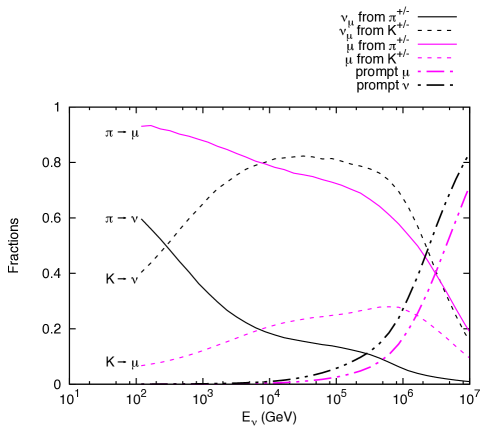
Figure 4: Relative contributions of pions, kaons and charmed hadrons to the fluxes of muon neutrinos compared to those for muons. See text for discussion.

Charmed hadrons have much shorter lifetimes, so their critical energies are more than $10$ PeV and their spectrum at high energy is one power less steep than the “conventional" neutrinos from decay of pions and kaons. Therefore, despite their small production cross sections, they eventually become the dominant source of atmospheric neutrinos, as shown by the lines for prompt neutrinos ($\nu_{\mu}+\overline{\nu}_{\mu}$) in Fig. 3. The yields of $nu_{e}$, $\nu_{\mu}$ and $\mu$ are approximately equal in decays of charmed mesons. However, the prompt muon flux includes an additional contribution from decay of unflavored mesons [48, 40]. Nevertheless, the prompt fraction for muons is lower than that for $\nu_{\mu}$ because the conventional muon flux is significantly higher than the conventional $\nu_{\mu}$ flux.

Electron neutrinos at high energy come primarily from three-body decays of charged and neutral kaons. Their flux at high energy is about 5% of the flux of muon neutrinos. Fluxes of $\nu+\overline{\nu}$ averaged over zenith angle are shown in Fig. 3 separately for conventional and for prompt neutrinos. Calculation of the flux of conventional atmospheric $\nu_{e}$ is reviewed in Ref. [47], which includes the very small contribution from K_S that is analogous to the prompt contribution because of its short lifetime. The flux of atmospheric $\nu_{\tau}$ is much smaller than $\nu_{\mu}$ and $\nu_{e}$. They come mainly from decay of $D_{s}$ [49].

0.2.2 Muon charge ratio and $\nu_{\mu}\,/\,\overline{\nu}_{\mu}$

Atmospheric muons are closely related to neutrinos and are much easier to measure. For this reason, observations of muons can place useful constraints on atmospheric neutrinos. Indeed, one approach is to calculate the flux of $\nu_{\mu}$ from measurements of muons at high altitude [50]. The Honda group [51, 52] used measurements of atmospheric muons at various atmospheric depths to tune the interaction model of their original three dimensional calculation [7]. A limitation to this approach at TeV energies is that the neutrinos come much more from the kaon channel, which gives a relatively small contribution to the muons. In this connection, it is relevant to note that there is a feature in the muon charge ratio that directly reflects the kaon contribution and can be used to constrain the parameter related to kaon production. The $\mu^{+}/\mu^{-}$ ratio increases in the energy range approaching a TeV (see Fig. 5) as the pion contribution steepens for $E>\epsilon_{\pi}\approx 115$ GeV. This increase reflects the associated production channel, $p\rightarrow\Lambda K^{+}$, the isospin conjugate of which ($n\rightarrow\Lambda K^{0}$) does not produce corresponding $\mu^{-}$s.

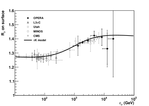
Figure 5: Muon charge ratios as a function of energy. The figure is from OPERA [53]. The line shows their fit to the data using the parameterization of Ref. [54].

Calculating the muon charge ratio requires keeping track separately of protons and neutrons in the primary spectrum and following the charges separately in solving the cascade Eq. 0.2. The effect of the proton excess in the primary spectrum of nucleons is contained in the parameter $\delta_{0}\equiv(p-n)/(p+n)$, which decreases with energy up to energies approaching a PeV, as shown in the left panel of Fig. 6. For pions, relatively simple solutions for $\Pi^{+}(E,X)\pm\Pi^{-}(E,X)$ can be obtained [55] in terms of $\beta\equiv(1-Z_{pp}-Z_{pn})/(1-Z_{pp}+Z_{pn})$ and $\alpha_{\pi}\equiv(Z_{p\pi^{+}}-Z_{p\pi^{-}})/(Z_{p\pi^{+}}+Z_{p\pi^{-}})\approx 0.17.$ Separate solutions for $K^{+}$ and $K^{-}$ are more complicated because the charged kaons are not isospin conjugates of each other. In the more general calculation that tracks $K^{\pm}$ separately as well as $\pi^{\pm}$ [54], the main parameter for kaons is $\alpha_{K}\equiv(Z_{pK^{+}}-Z_{pK^{-}})/(Z_{pK^{+}}+Z_{pK^{-}})\approx 0.51$. The larger charge ratio for kaons shows up in the TeV range as the kaon contribution to the muon flux increases relative to that of the pions. The OPERA group fit their data with the parameterization of Ref. [54] using two free parameters. They find $\delta_{0}=0.61\pm 0.02$ and $Z_{pK^{+}}=0.0086\pm 0.0004$ at $E_{\mu}\approx 2$ TeV, which corresponds to a primary energy per nucleon higher by roughly a factor of ten. Their fit to the $\mu^{+}/\mu^{-}$ ratio is shown by the line in Fig. 5. The OPERA paper also points out that the prompt contribution to the muon flux has a charge ratio of one so that the charge ratio will decrease at energies so high that prompt muons contribute significantly.

 

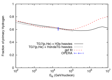
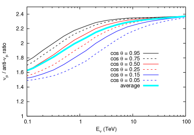
Figure 6: Left: Proton excess in the spectrum of nucleons. The fitted value of OPERA [53] is placed at $20$ TeV primary energy, corresponding to $\sim 2$ TeV muon energy. Spectrum fits are discussed in § 0.3; Right: Ratio of $\nu_{\mu}/\overline{\nu}_{\mu}$ as a function of energy and zenith angle calculated with the parameterization of Ref. [54] with $\delta_{0}$ and $Z_{pK^{+}}$ fit by OPERA [53]

Because the kaon channel dominates the production of muon neutrinos, the $\nu_{\mu}\,/\,\overline{\nu}_{\mu}$ ratio is significantly higher than the charge ratio of muons. The ratios for muon neutrinos are shown in Fig. 6 (right) with the parameters of[54] as modified by OPERA. The evolution to the high-energy plateau occurs faster for near vertical directions than for the horizontal, reflecting the $\cos\theta E_{\nu}\,/\,\epsilon_{K}$ factor in the denominator of Eq. 0.2.1. Different hadronic interaction models predict significantly different values for the $\nu_{\mu}\,/\,\overline{\nu}_{\mu}$ ratio [38]. Although all show the increase with energy associated with the higher charge ratio for kaons, the magnitudes in the TeV range vary by a factor of two among the models. The connection to the measured muon charge ratio is potentially valuable in this context, but has yet to be fully exploited.

0.2.3 Seasonal variations

Rates of high-energy muons exhibit a seasonal variation correlated with the temperature in the upper atmosphere where most of the production occurs. The effect was first measured and understood in the underground muon experiment at Cornell [56]. The variation is a direct consequence of the fact that the meson decay rate in Eq. 6 is proportional to temperature combined with the fact that the probability for re-interaction before decay increases with energy. For example, when $\cos\theta\,E_{\mu}>>\epsilon_{\pi}$ in the muon analog of Eq. 0.2.1, then the d$N_{\mu}$/d$E_{\mu}\propto\epsilon_{\pi}\propto T$. In this limit, the pion contribution to the muon flux is fully correlated with the temperature. For $\cos\theta\,E_{\mu}<<\epsilon_{\pi}$, the temperature-dependent term is negligible, most mesons decay before they interact and the temperature dependence disappears for low energy. There is an intermediate region in the TeV range where the pion contribution is asymptotic, but the kaon contribution is not, so the details of the seasonal variation are in principle sensitive to the ratio of charged pions to kaons in hadronic interactions. For $E_{\mu}\leq 1$ PeV the contribution from prompt muons should not depend on temperature because of the large critical energy of D mesons.

  

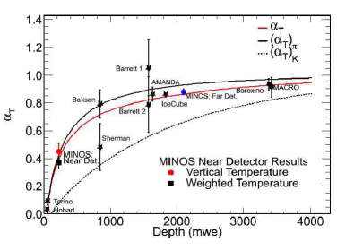
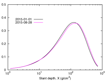
Figure 7: Left: Summary of measurements of the correlation coefficient between muon rate and effective temperature from Ref. [57]; Right: Normalized production spectrum of muons at a zenith angle of $30^{\circ}$.

The connection between muon rate and temperature is characterized by a correlation coefficient defined in the relation

$$\frac{\delta\phi(E_{\mu})}{\phi(E_{\mu})}=\alpha_{T}\frac{\delta T}{T}.$$ (11)

Following the argument in the previous paragraph, the correlation coefficient should rise from a small value at low energy and approach unity at high energy, with a possible decrease in the PeV range corresponding to the onset of prompt muons [58]. This expected rise from shallow detectors ($E_{\mu}\approx 50$ GeV, at the MINOS near detector [57]) through IceCube [59] and the MINOS far detector at Soudan [60] ($\sim$ TeV) to MACRO [61] ($\sim$ 2TeV) is nicely illustrated in the compilation of data in Ref. [57], reproduced here in the left panel of Fig. 7.

An experimental determination of the correlation coefficient requires integrating the atmospheric temperature profile weighted by the production spectrum of muons and the energy and angular dependence of the detector response to determine an effective temperature,

$$T_{\rm eff}(\theta)=\frac{\int{\rm d}E_{\mu}A_{\rm eff}(E_{\mu},\theta)\int{\rm d}XP_{\mu}(E_{\mu},\theta,X)T(X)}{\int{\rm d}E_{\mu}A_{\rm eff}(E_{\mu},\theta)\int{\rm d}XP_{\mu}(E_{\mu},\theta,X)}.$$ (12)

Here $A_{\rm eff}$ is the detector acceptance (area x solid angle) for detecting muons of energy $E_{\mu}$ at production from zenith angle $\theta$, and $P_{\mu}$ is the production spectrum of muons at slant depth X(g/cm²). $T_{\rm eff}$ is obtained after averaging over zenith angle. As an example, the production profile $P_{\mu}(E_{\mu},\theta,X)$ at 30^∘ is shown in the right panel of Fig. 7. The muon production profile itself depends only slightly on the temperature profile (through the temperature dependence of the critical energy). The examples in the figure correspond to $T_{\rm eff}=-37^{\circ}C$ on 2015-Jan-01 and $-81^{\circ}C$ on 2015-Aug-28 at the South Pole.

The contributions of pions and kaons are combined in Eq. 12 and in the red curve in the left panel of Fig. 7.  The contributions for pions only (solid black line) and for kaons only (broken black line) are also shown separately in the figure. Because of the relatively higher contribution of kaons to muon neutrinos, the correlation coefficient for neutrinos is expected to be significantly lower than that for muons. A study by IceCube using upward neutrinos from the partially completed detector[63] finds $\alpha_{T}^{\nu}\approx 0.5$ with large uncertainties. The study uses events with zenith angles $120^{\circ}\leq\theta\leq 90^{\circ}$ corresponding to latitudes between $-30^{\circ}$ and $-90^{\circ}$, so the seasonal phase of the temperature dependence can be compared with that of muons in IceCube produced in the atmosphere above the South Pole.

0.3 Primary spectrum

Direct measurements of the cosmic-ray spectrum with spectrometers in space now extend to a rigidity of $\approx 2$ TV, corresponding to $E\sim$TeV/nucleon. Measurements with balloon-borne calorimeters now approach $100$ TeV/nucleon. Information at higher energies is provided by data from extensive air shower (EAS) experiments, which do not directly detect the primary nuclei. They generally measure the all-particle spectrum; that is, the spectrum in terms of energy per particle. Composition of the primary beam is determined indirectly from properties of the cascade such as depth of shower maximum and ratio of electrons/photons to muons in the shower. The composition is at best determined to the level of five groups of nuclei: proton, helium, CNO, Si-Mg and Fe. Conversion to the spectrum of nucleons in terms of energy per nucleon, which is needed for calculation of fluxes of neutrinos, therefore becomes more uncertain for $E>100$ TeV.

For calculations of the flux of atmospheric neutrinos it is useful to have a parameterization of the primary spectrum anchored to direct measurements at low energy and guided by the principle of rigidity dependence to account for the knee of the spectrum. The Polygonato Model [65] is the classic example, with each and every element characterized by a normalization and spectral index at low energy and extrapolated to air shower energies ($\sim PeV$). A rigidity-dependent change of slope is assumed to characterize the steepening of the spectrum around $3$ PeV. The fact that both propagation and acceleration of cosmic rays depend on magnetic rigidity justifies the assumption that features in the spectrum should occur at the same rigidity for all nuclei. Rigidity is $Pc\,/\,Ze$, which is the total energy per particle divided by its charge. A consequence of the rigidity dependence is that the steepening of the different elements occurs in a sequence known as the Peters Cycle [66], with protons first, followed by He, CNO, etc. If the knee is characterized by a rigidity $R_{c}\approx 4\times 10^{6}$ GV, then the steepening occurs at total energy per particle

$$E_{tot}^{c}\,=\,A\times E_{N,c}\,=\,Ze\times R_{c},$$ (13)

where $A$ and $Z$ are the mass and charge of a nucleus with energy per nucleon $E_{N}$.

A simplified but extended version of the Polygonato Model is H3a [54]. It is “simplified" to consist of the standard five groups of nuclei rather than individual elements, and “extended" to three populations of particles, a Galactic component that cuts off at the knee, a second Galactic component, and an extra-galactic component. Hillas [67] pointed out that, if the ankle of the spectrum around $3$ EeV signals the onset of the extra-galactic population, then a second Galactic component is needed to fill in the gap after the heavy component of the first population turns down around $100$ PeV. Fig. 9 illustrates the need for a second Galactic component (or a low-energy extension of the extra-galactic component).

  

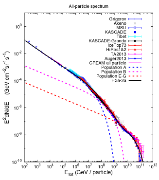
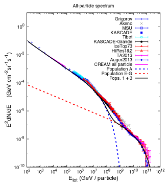
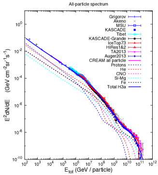
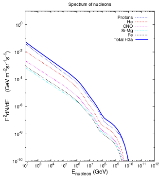
Figure 8: Left: All-particle spectrum showing separately the contribution of three populations in a modified H3a model (see text); Right:All-particle spectrum with the second Galactic population omitted.

  

Figure 9: Left: all-particle spectrum showing separately the contribution of five mass groups in a modified H3a model (see text); Right: spectrum of nucleons corresponding to all-particle spectrum.

In such a model, the contribution to the all particle spectrum of nuclear group $i$ is

$$\Phi_{i}(E)\,\equiv\,E\frac{{\rm d}N_{i}}{{\rm d}E}\,=\,\sum_{j=1}^{3}a_{i,j}E^{-\gamma_{i,j}}\times exp\left\{-\frac{E}{Z_{i}R_{c,j}}\right\},$$ (14)

where $\gamma_{i,j}$ is the integral spectral index for nuclear group $i$ in Population $j$. The spectrum is written here as $\Phi={\rm d}N/{\rm d}\ln E$ to simplify the Jacobian for the transition to the spectrum of nucleons, but also because cosmic-ray spectral measurements are invariably presented as number of events per logarithmic interval of energy. Thus the spectrum of nucleons is

$$\Phi_{N}(E_{N})\,\equiv\,E_{N}\frac{{\rm d}N}{{\rm d}E_{N}}\,=E_{N}\phi(E_{N})\,=\,\sum_{i=1}^{5}A_{i}\times\Phi_{i}(A_{i}E_{N}).$$ (15)

The all-particle spectrum and the corresponding spectrum of nucleons are shown side by side in Fig. 9. Because of the steep spectrum, the contributions of nuclei to the spectrum of nucleons are suppressed. Note in particular that helium, which has a harder spectrum than protons and crosses above protons in the all-particle spectrum, is always subdominant in the spectrum of nucleons. Contributions of heavier nuclei are even smaller.

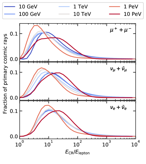
Figure 10: Distributions of primary energy per nucleon for atmospheric leptons. (From Ref.[40])

Figure 10 from Ref.[40] shows the distribution of primary energies per nucleon ($E_{N}$) that produce leptons of energy $E_{\ell}$ as a function of the ratio of the energies. The distributions reflect the underlying ratios of $E_{N}/E_{m}$ and $E_{m}/E_{\ell}$ and the steepness of the cosmic-ray spectrum (m$=\pi^{\pm},\,K^{\pm},\,D$). For $E_{\ell}\approx 1$ PeV, the steeper spectrum above the knee shifts the primary energy down. For $10$ TeV, the prompt component dominates and the distributions reflect the kinematics of charm decay for neutrinos and also the unflavored component for muons. At lower energies, the curves for $\mu$ and $\nu_{e}$ approximately scale, while those for $\nu_{\mu}$ reflect the transition to dominance of the kaon channel.

0.3.1 Direct measurements and Population 1

Early measurements [68, 69] with the CREAM balloon calorimeter were used to determine the parameters $a_{i,1}$ and $\gamma_{i,1}$ of the first population in H3a. There are now direct measurements with spectrometers from PAMELA [70] and AMS02 [71, 72] as well as a recent measurement by CREAM [73]. In their measurements of protons and helium, PAMELA confirmed what CREAM [69] called a “discrepant hardening" of the elemental spectra. The hardening of the spectrum above 200 GV rigidity has now been measured by AMS02 [74] for helium, carbon and oxygen, as well as for protons [71].

A theoretical interpretation [75, 76] is that below $\approx 200$ GV propagation of cosmic rays in the Galaxy in dominated by turbulence self-generated by the cosmic rays, which gives a relatively soft spectrum. Then there is a transition at high rigidity to a regime in which the propagation is dominated by external turbulence, for example, turbulence driven by supernova explosions. The observed spectral index is the combination of the injection spectrum at the sources and the energy dependence of diffusion, $\gamma=\gamma_{s}+\delta(R)$. In this picture, $\delta(R<200)>\delta(R>200)$, and the high energy behavior can be expected to apply up to the knee. Fits to AMS02 data for protons [71] and helium [72] (Fig. 11) have been used for the first population in a revised H3a model for the extrapolation to the knee. Cosmic-ray spectrum figures in this paper are made with this revision.

  

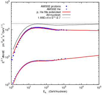
Figure 11: Left: Extrapolation of AMS02-data for protons and helium to high energy, with Helium plotted as number of nuclei per energy per nucleon; Right: Fractional contributions to the spectrum of nucleons. Protons and He are from AMS02 [71, 72]; heavier nuclear groups are from Ref. [9].

The proton and helium data below $10$ GeV are strongly affected by solar modulation, so the fits in Fig. 11 require parameterizations that account for the characteristic suppression at low energy. For high energy, they also require a form that changes the slope. A seven parameter form suggested by Evans et al. [77] is used:

$$\frac{{\rm d}n}{{\rm d}E_{k}}=a\left[E_{k}+b\exp\left(-c\sqrt{E_{k}}\right)\right]^{-\alpha_{1}}\times\left[1+\left(\frac{E_{k}}{E_{c}}\right)^{s}\right]^{\frac{\alpha_{1}-\alpha_{2}}{s}}.$$ (16)

The first factor is the form [78, 9] based on direct measurements and used for several of the atmospheric neutrino calculations that include solar modulation at low energy and extend to $E_{\nu}=10$ TeV. The second factor is the form originally suggested in [80] to make a smooth parameterization of the steepening at the knee of the spectrum (see also [81]). Here it provides the transition from a steeper to a harder power ($\alpha_{2}<\alpha_{1}$) at a rigidity $\approx 240$ GV. In Ref. [77] Eq. 16 was used to fit several proton data sets. Here it is based specifically on the AMS02 measurements of protons and helium with the parameters in Table 2.

Table 2: Parameters for Eq. 16.

	$a$ (m-2sr-1s-1)	$b$	$c$ (GeV${}^{-\frac{1}{2}}$)	$E_{c}$ (GeV)	$s$	$\alpha_{1}$	$\alpha_{2}$
p	$2.17\times 10^{4}$	2.4	0.12	240.	3.56	2.845	2.71
He	800.	2.0	0.33	122.	3.5	2.72	2.63

0.3.2 Neutrino flux from a non-power-law spectrum

In order to calculate the spectrum of neutrinos over a wide energy range, it is necessary to take account of deviation of the primary spectrum from the power-law behaviour assumed for Eq. 0.2.1. To do so in the framework of the analytic approach used here, it is necessary to use energy-dependent spectrum weighted moments as described in Ref. [82]. For K⁺ production, for example, the generalization of

$$Z_{pK^{+}}=\int_{0}^{1}\,x^{\gamma}\frac{{\rm d}n_{K^{+}}(x)}{{\rm d}x}$$

is

$$Z_{NK^{+}}(E)\,=\,\int_{E}^{\infty}\,{\rm d}E^{\prime}\frac{\phi_{N}(E^{\prime})}{\phi_{N}(E)}\frac{\lambda_{N}(E)}{\lambda_{N}(E^{\prime})}\frac{{\rm d}n_{K^{+}}(E^{\prime},E)}{{\rm d}E}.$$ (17)

As this equation makes clear, this anzatz builds in energy dependence of interaction and production cross sections as well as the deviation from a power-law spectrum. However, its implementation requires full knowledge of the hadronic production cross sections as a function of beam energy $E^{\prime}$ for the full phase space of secondary energy $E$.

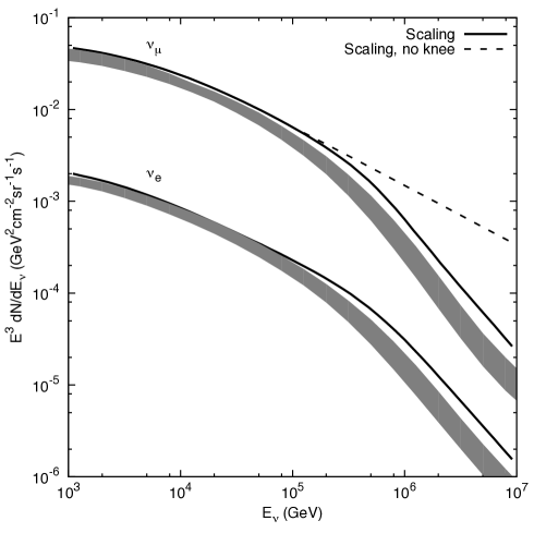
Figure 12: Shaded bands show the range of uncertainties in the angle-averaged neutrino fluxes for several models of hadronic interactions. The solid line shows for comparison the flux from a calculation in which the spectrum weighted moments are constant and the only source of energy dependence is from the spectrum. The dashed line shows the flux for a single power-law spectrum with no knee.

An approximate scheme for handling energy-dependent production cross sections is worked out in Ref. [83]. It uses two-parameter fits for the production cross sections [84] of the form $dn_{ji}/dx=c_{ji}(E)(1-x)^{p_{ji}(E)}\,/\,x$ at closely spaced intervals of energy to obtain the energy dependence of the $c$ and $p$ parameters. This procedure is used in a subsequent paper [85] to compare atmospheric neutrino fluxes for a range of interaction models and primary spectra. The main conclusion is that the variations due to different representations of the knee in the primary spectrum for a given interaction model are not as large as variations among different hadronic interaction models for a given primary spectrum. The uncertainty range for conventional neutrinos from several interaction models is shown in Fig. 12. The shaded bands include Sib2.1 [86], EPOS-LHC [87], QGSJet II-04 [88] and Sib 2.3 [43]. The variation is $\approx\pm 15$% from 1 to 30 TeV, increasing to $\approx\pm 40$% above in the PeV range. The corresponding ranges for differences in primary spectra are $\pm 10$% to $\pm 15$%.

These ranges of uncertainties should be compared with an extensive evaluation of uncertainties in lepton fluxes in Ref. [89]. An earlier assessment of uncertainties in fluxes of high-energy atmospheric muons only is Ref. [90].

0.4 Atmospheric neutrinos with $E_{\nu}>10$ TeV

IceCube has discovered a diffuse flux of astrophysical neutrinos from the whole sky [91, 92] by selecting events that start well inside its deep array of optical modules. This high-energy starting event (HESE) sample includes both tracks initiated by charged current (CC) interactions of $\nu_{\mu}$ and cascades from $\nu_{e}$, $\nu_{\tau}$ and neutral current interactions of all flavors. The cascade sample also includes some $\nu_{\mu}$ charged current events in which most of the energy is given to the nuclear fragmentation. The energy threshold is $30$ TeV. The starting event analysis is extended to lower energy ($\sim$TeV) by progressively increasing the outer veto region [93]. Neutrinos of astrophysical origin are also detected [94] above the steeply falling background of atmospheric neutrinos from analysis of upward tracks, most of which start from CC interactions of $\nu_{\mu}$ in the rock and ice outside the detector. In both cases, it is important to understand the background of atmospheric neutrinos.

  

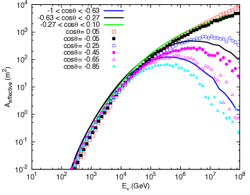
Figure 13: Left: Diagram showing absorption of muon neutrinos by the Earth; Right: Effective area for upward neutrinos in IceCube. (See text for explanation.)

0.4.1 Upward neutrino-induced muons

Selecting upward moving tracks uses the Earth as a filter to remove all backgrounds except atmospheric $\nu_{\mu}$.

Transparency of the Earth

In this case it is necessary to understand the dependence of absorption by the Earth as a function of zenith angle and neutrino energy. Figure 13 (left) shows how the Earth shadows upward-moving neutrinos. The solid line shows the thickness of the Earth as a function of direction [95]. The dashed lines show the fraction of neutrinos absorbed for selected neutrino energies. Absorption affects both astrophysical and atmospheric neutrinos. It starts to become important for $E_{\nu}\approx 10$ TeV. For higher energies, increasing absorption limits trajectories to near the horizon. For conventional atmospheric neutrinos, absorption enhances the intrinsic preference for large angles from the $\sec\theta$ effect.

Effective areas for upward $\nu_{\mu}$

The effective area is a detector-dependent quantity that connects a flux of neutrinos with the observed signal. For upward muon neutrinos $\phi_{\nu}\times A_{\rm eff}$ gives the observed rate of neutrino-induced muons. The effective area for this case is given by

$$A_{\rm eff}(E_{\nu},\theta)\,=\,\epsilon(E_{\rm th},\theta)\,A(\theta)\,P_{\nu}(E_{\nu},E_{\mu}>E_{\rm th})\,\exp\{-(1-\zeta)\sigma_{\nu}(E_{\nu})N_{A}X(\theta)\}.$$ (18)

Effects of absorption in the Earth are reflected in the exponential absorption factor where $X(\theta)$ is the slant depth through the Earth in g/cm², $N_{A}$ is the number of nucleons per gram, $\sigma_{\nu}$ the total neutrino cross section and $\zeta$ accounts for energy loss and regeneration in NC interactions. [96]. The efficiency of the detector $\epsilon(E_{\rm th},\theta)$ for measuring a muon above some threshold energy from direction $\theta$ multiplied by its projected area $A(\theta)$ sets the scale. The central factor in Eq. 18, $P(E_{\nu},E_{\mu}>E_{\rm th})$, is the probability that a muon neutrino (or antineutrino) of energy $E_{\nu}$ headed toward the detector will produce a muon that reaches it with $E_{\mu}>E_{\rm th}$.

Effective areas for the measurement of diffuse, upward muon neutrinos by IceCube [94] are shown by the full lines in the right panel of Fig. 13 for three ranges of zenith angle. The broken lines show the effective area for upward neutrinos in the IceCube point source search.[101]

0.4.2 Starting events and neutrino self-veto

The stating event analyses in IceCube  [91, 92] depend on a veto region to exclude entering muons and select only neutrino interaction vertices well inside the detector. This has an important effect on the atmospheric neutrino background from above the detector: neutrinos accompanied by muons at the detector will be classified as muons and therefore excluded from the neutrino sample. Only those atmospheric neutrinos that are not accompanied by a muon at the detector will be included. This self-veto effect increases with energy because the likelihood that a muon produced in the same event has sufficient energy to reach the deep detector increases. The flux of atmospheric neutrinos at the detector is then expressed as

$$\phi_{\nu,{\rm det}}(E_{\nu},\theta)={\cal P}_{i}(E_{\nu},E_{\mu}^{\rm min},\theta)\phi_{\nu}(E_{\nu},\theta),$$ (19)

where the passing rate ${\cal P}_{i}$ depends on neutrino flavor ($i$), energy and angle and on the depth of the detector through $E_{\mu}^{\rm min}$. The passing rate is lowest at the zenith and increases to unity at the horizon as the energy required of the muon to reach the detector increases because of the larger slant depth. This introduces an additional angular dependence to the atmospheric neutrino distributions at the detector, favoring large angle more and more as energy increases, as shown in Fig. 14 (left). Unlike the increased enhancement toward the horizon in the case of upward $\nu_{\mu}$, which affects both atmospheric and astrophysical neutrinos, here it is only the atmospheric neutrinos that are affected. Thus the energy and angular dependence of ${\cal P}_{i}$ in the case of neutrinos from above provide additional discrimination power between astrophysical and atmospheric neutrinos.

  

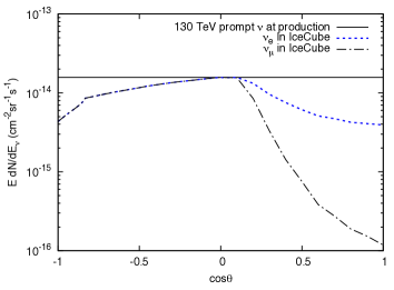
Figure 14: Left: Angular dependence of fluxes of conventional muon neutrinos at three energies, with shaded regions showing the effect of the neutrino self-veto; Right: Angular dependence of prompt neutrinos at 130 TeV, with full lines showing the distributions at production and broken lines the flux at the center of IceCube after absorption by the Earth ($\cos\theta<0.$) and after applying the passing fraction of Ref.[36].

For a given energy and angle the passing fraction is much smaller for $\nu_{\mu}$ than for $\nu_{e}$ because of the muon that is produced in the same decay as the $\nu_{\mu}$. The contribution to the passing fraction from the sibling muon was calculated in Ref. [102] in the analytic framework of Ref. [42] by adding the requirement $E_{\mu}>E_{\mu}^{\rm min}$ to the integrals of pion and kaon decay in the neutrino production spectrum. The calculation illustrated the point that the passing fraction increases with the depth of the detector because $E_{\mu}^{\rm min}$ is larger.

To generalize the calculation of the passing rate to include the case in which the vetoing muon is produced elsewhere in the shower requires integrating over the properly weighted distribution of primary cosmic-rays capable of producing the target neutrino. For each step of the integral, the probability that a cosmic-ray of the given energy will produce a muon with $E_{\mu}>E_{\mu}^{\rm min}$ is accumulated. In this way a generalized passing fraction is calculated that applies also to electron neutrinos and which, when combined with the analytic estimate, slightly reduces the passing fraction for muon neutrinos. The generalized self-veto was first implemented in Ref. [103] using the Elbert formula [104, 105] to evaluate the muons produced elsewhere in the shower. The original parameters of the Elbert formula were tuned to improve agreement with a limited set of Monte Carlo calculations. This passing fraction was applied to the IceCube $>1$ TeV starting event analysis [93] and to the four- [106] and six-year [107] HESE analyses with $E_{\mu}^{\rm min}$ calculated so that the vetoing muon has $1$ TeV at the detector.

A recent paper [36] unifies and improves the accuracy of the passing fraction in several ways. The MCEq [39] program is used to evaluate muons produced elsewhere in the shower, taking account of the energy removed from the primary cosmic-ray by the neutrino. Fluctuations in muon energy loss are accounted for, which smooths out the shoulder in the passing fraction for the sibling muon visible in the plots of Ref. [102]. The numerical calculations are compared to an application specific Monte Carlo [37] designed to evaluate neutrino fluxes efficiently. The comparison confirms an interesting feature of the calculation, which is that passing fractions for conventional anti-neutrinos are slightly lower than for conventional neutrinos. This is attributed to the fact that negative mesons, and therefore their decay products including anti-neutrinos, on average carry a smaller fraction of the primary energy, leaving more energy in the rest of the shower to provide a vetoing muon. The passing rates are tabulated over a range of energies and directions extending to very low values for high energy and directions near the vertical. For the purpose of evaluating the shape and level of the surviving atmospheric neutrinos, passing rates much less than the fractional uncertainties from treatment of hadronic interactions and the primary spectrum are equivalent to zero. In the case of a very high energy astrophysical candidate, however, it may be important to have a precise knowledge of a very small passing probability.

The combination of absorption in the Earth for upward events and the self-veto effect for downward events provides a distinctive energy-dependent signature for prompt neutrinos, as illustrated in the right panel of Fig. 14. The energy chosen in the plot is the crossover region between prompt and atmospheric electron neutrinos. The challenge is that the expected rates of prompt $\nu_{e}$ in the HESE analysis are low [83].

0.5 Concluding comment

The analytic/numerical approach illustrated in this chapter remains useful for insight into the physics and phenomenology of atmospheric lepton fluxes. It can also provide the basis for quantitative estimates of their uncertainties.

References

References

- [1] Super-Kamiokande collaboration, Y. Fukuda et al., Evidence for oscillation of atmospheric neutrinos, Phys. Rev. Lett. 81 (1998) 1562–1567, [hep-ex/9807003].
- [2] G. Barr, T. K. Gaisser and T. Stanev, Flux of Atmospheric Neutrinos, Phys. Rev. D39 (1989) 3532–3534.
- [3] V. Agrawal, T. K. Gaisser, P. Lipari and T. Stanev, Atmospheric neutrino flux above 1-GeV, Phys. Rev. D53 (1996) 1314–1323, [hep-ph/9509423].
- [4] M. Honda, K. Kasahara, K. Hidaka and S. Midorikawa, Atmospheric neutrino fluxes, Phys. Lett. B248 (1990) 193–198.
- [5] M. Honda, T. Kajita, K. Kasahara and S. Midorikawa, Calculation of the flux of atmospheric neutrinos, Phys. Rev. D52 (1995) 4985–5005, [hep-ph/9503439].
- [6] G. Battistoni, A. Ferrari, P. Lipari, T. Montaruli, P. R. Sala and T. Rancati, A Three-dimensional calculation of atmospheric neutrino flux, Astropart. Phys. 12 (2000) 315–333, [hep-ph/9907408].
- [7] M. Honda, T. Kajita, K. Kasahara and S. Midorikawa, A New calculation of the atmospheric neutrino flux in a 3-dimensional scheme, Phys. Rev. D70 (2004) 043008, [astro-ph/0404457].
- [8] G. D. Barr, T. K. Gaisser, P. Lipari, S. Robbins and T. Stanev, A Three - dimensional calculation of atmospheric neutrinos, Phys. Rev. D70 (2004) 023006, [astro-ph/0403630].
- [9] T. K. Gaisser and M. Honda, Flux of atmospheric neutrinos, Ann. Rev. Nucl. Part. Sci. 52 (2002) 153–199, [hep-ph/0203272].
- [10] Soudan 2 collaboration, M. C. Sanchez et al., Measurement of the L/E distributions of atmospheric neutrinos in Soudan 2 and their interpretation as neutrino oscillations, Phys. Rev. D68 (2003) 113004, [hep-ex/0307069].
- [11] MACRO collaboration, M. Ambrosio et al., Atmospheric neutrino oscillations from upward through going muon multiple scattering in MACRO, Phys. Lett. B566 (2003) 35–44, [hep-ex/0304037].
- [12] Super-Kamiokande collaboration, E. Richard et al., Measurements of the atmospheric neutrino flux by Super-Kamiokande: energy spectra, geomagnetic effects, and solar modulation, Phys. Rev. D94 (2016) 052001, [1510.08127].
- [13] IceCube collaboration, M. G. Aartsen et al., Measurement of Atmospheric Neutrino Oscillations at 6-56 GeV with IceCube DeepCore, Phys. Rev. Lett. 120 (2018) 071801, [1707.07081].
- [14] N. Jelley, A. B. McDonald and R. G. H. Robertson, The Sudbury Neutrino Observatory, Ann. Rev. Nucl. Part. Sci. 59 (2009) 431–465.
- [15] Daya Bay collaboration, F. P. An et al., Observation of electron-antineutrino disappearance at Daya Bay, Phys. Rev. Lett. 108 (2012) 171803, [1203.1669].
- [16] RENO collaboration, J. K. Ahn et al., Observation of Reactor Electron Antineutrino Disappearance in the RENO Experiment, Phys. Rev. Lett. 108 (2012) 191802, [1204.0626].
- [17] Double Chooz collaboration, Y. Abe et al., Reactor electron antineutrino disappearance in the Double Chooz experiment, Phys. Rev. D86 (2012) 052008, [1207.6632].
- [18] K2K collaboration, M. H. Ahn et al., Measurement of Neutrino Oscillation by the K2K Experiment, Phys. Rev. D74 (2006) 072003, [hep-ex/0606032].
- [19] MINOS collaboration, P. Adamson et al., Measurement of Neutrino and Antineutrino Oscillations Using Beam and Atmospheric Data in MINOS, Phys. Rev. Lett. 110 (2013) 251801, [1304.6335].
- [20] T2K collaboration, K. Abe et al., Measurement of Neutrino Oscillation Parameters from Muon Neutrino Disappearance with an Off-axis Beam, Phys. Rev. Lett. 111 (2013) 211803, [1308.0465].
- [21] Super-Kamiokande collaboration, K. Abe et al., Atmospheric neutrino oscillation analysis with external constraints in Super-Kamiokande I-IV, Phys. Rev. D97 (2018) 072001, [1710.09126].
- [22] Particle Data Group collaboration, K. A. Olive, K. Nakamura, S. Petcov et al., Review of Particle Physics; Neutrino Mass, Mixing and Oscillations, Chin. Phys. C38 (2014) 235,258.
- [23] Particle Data Group collaboration, M. Tanabashi, K. Nakamura, S. Petcov et al., Review of Particle Physics, Phys. Rev. D98 (2018) 030001.
- [24] Super-Kamiokande collaboration, K. Abe et al., Evidence for the Appearance of Atmospheric Tau Neutrinos in Super-Kamiokande, Phys. Rev. Lett. 110 (2013) 181802, [1206.0328].
- [25] OPERA collaboration, N. Agafonova et al., Final Results of the OPERA Experiment on Appearance in the CNGS Neutrino Beam, Phys. Rev. Lett. 120 (2018) 211801, [1804.04912].
- [26] T. DeYoung, Latest Neutrino Physics Results from IceCube and ANTARES, Neutrino 2018 .
- [27] J. G. Learned and S. Pakvasa, Detecting tau-neutrino oscillations at PeV energies, Astropart. Phys. 3 (1995) 267–274, [hep-ph/9405296].
- [28] G. D. Barr, T. K. Gaisser, S. Robbins and T. Stanev, Uncertainties in Atmospheric Neutrino Fluxes, Phys. Rev. D74 (2006) 094009, [astro-ph/0611266].
- [29] HARP collaboration, M. G. Catanesi et al., Measurement of the production cross-sections of in p-C and -C interactions at 12 GeV/c, Astropart. Phys. 29 (2008) 257–281, [0802.0657].
- [30] NA49 collaboration, C. Alt et al., Inclusive production of charged pions in p+C collisions at 158-GeV/c beam momentum, Eur. Phys. J. C49 (2007) 897–917, [hep-ex/0606028].
- [31] NA49 collaboration, T. Anticic et al., Inclusive production of protons, anti-protons and neutrons in p+p collisions at 158-GeV/c beam momentum, Eur. Phys. J. C65 (2010) 9–63, [0904.2708].
- [32] NA61/SHINE collaboration, N. Abgrall et al., Measurement of negatively charged pion spectra in inelastic p+p interactions at = 20, 31, 40, 80 and 158 GeV/c, Eur. Phys. J. C74 (2014) 2794, [1310.2417].
- [33] NA61/SHINE collaboration, A. Aduszkiewicz et al., Measurements of , K± , p and spectra in proton-proton interactions at 20, 31, 40, 80 and 158 with the NA61/SHINE spectrometer at the CERN SPS, Eur. Phys. J. C77 (2017) 671, [1705.02467].
- [34] G. T. Zatsepin and V. A. Kuz’min, Neutrino Production in the Atmosphere, Sov. Phys. JETP 14 (1961) 1294–1300.
- [35] L. V. Volkova, Energy Spectra and Angular Distributions of Atmospheric Neutrinos, Sov. J. Nucl. Phys. 31 (1980) 784–790.
- [36] C. A. Argüelles, S. Palomares-Ruiz, A. Schneider, L. Wille and T. Yuan, Unified atmospheric neutrino passing fractions for large-scale neutrino telescopes, arXiv:1805.11003 (2018) , [1805.11003].
- [37] K. Jero, CORSIKA modifications for faster background generation, EPJ Web Conf. 116 (2016) 02003.
- [38] A. Fedynitch, Phenomenology of atmospheric neutrinos, EPJ Web Conf. 116 (2016) 11010.
- [39] A. Fedynitch, https://github.com/afedynitch/MCEq, .
- [40] A. Fedynitch, F. Riehn, R. Engel, T. K. Gaisser and T. Stanev, The hadronic interaction model Sibyll-2.3c and inclusive lepton fluxes, arXiv:1806.04140 (2018) , [1806.04140].
- [41] F. Riehn, H. P. Dembinski, R. Engel, A. Fedynitch, T. K. Gaisser and T. Stanev, The hadronic interaction model SIBYLL 2.3c and Feynman scaling, PoS ICRC2017 (2017) 301, [1709.07227].
- [42] T. K. Gaisser, R. Engel and E. Resconi, Cosmic Rays and Particle Physics. Cambridge University Press, 2016.
- [43] F. Riehn, R. Engel, A. Fedynitch, T. K. Gaisser and T. Stanev, A new version of the event generator Sibyll, PoS ICRC2015 (2016) 558, [1510.00568].
- [44] A. Bhattacharya, R. Enberg, M. H. Reno, I. Sarcevic and A. Stasto, Perturbative charm production and the prompt atmospheric neutrino flux in light of RHIC and LHC, JHEP 06 (2015) 110, [1502.01076].
- [45] PROSA collaboration, M. V. Garzelli, S. Moch, O. Zenaiev, A. Cooper-Sarkar, A. Geiser, K. Lipka et al., Prompt neutrino fluxes in the atmosphere with PROSA parton distribution functions, JHEP 05 (2017) 004, [1611.03815].
- [46] R. Gauld, J. Rojo, L. Rottoli, S. Sarkar and J. Talbert, The prompt atmospheric neutrino flux in the light of LHCb, JHEP 02 (2016) 130, [1511.06346].
- [47] T. K. Gaisser and S. R. Klein, A new contribution to the conventional atmospheric neutrino flux, Astropart. Phys. 64 (2015) 13–17, [1409.4924].
- [48] J. I. Illana, P. Lipari, M. Masip and D. Meloni, Atmospheric lepton fluxes at very high energy, Astropart. Phys. 34 (2011) 663–673, [1010.5084].
- [49] L. Pasquali and M. H. Reno, Tau-neutrino fluxes from atmospheric charm, Phys. Rev. D59 (1999) 093003, [hep-ph/9811268].
- [50] D. H. Perkins, A New calculation of atmospheric neutrino fluxes, Astropart. Phys. 2 (1994) 249–256.
- [51] T. Sanuki, M. Honda, T. Kajita, K. Kasahara and S. Midorikawa, Study of cosmic ray interaction model based on atmospheric muons for the neutrino flux calculation, Phys. Rev. D75 (2007) 043005, [astro-ph/0611201].
- [52] M. Honda, T. Kajita, K. Kasahara, S. Midorikawa and T. Sanuki, Calculation of atmospheric neutrino flux using the interaction model calibrated with atmospheric muon data, Phys. Rev. D75 (2007) 043006, [astro-ph/0611418].
- [53] OPERA collaboration, N. Agafonova et al., Measurement of the TeV atmospheric muon charge ratio with the complete OPERA data set, Eur. Phys. J. C74 (2014) 2933, [1403.0244].
- [54] T. K. Gaisser, Spectrum of cosmic-ray nucleons, kaon production, and the atmospheric muon charge ratio, Astropart. Phys. 35 (2012) 801–806, [1111.6675].
- [55] W. R. Frazer, C. H. Poon, D. Silverman and H. J. Yesian, Limiting fragmentation and the charge ratio of cosmic ray muons, Phys. Rev. D5 (1972) 1653–1657.
- [56] P. Barrett et al., Interpretation of cosmic-ray measurements far underground, Rev. Mod. Phys. 24 (1952) 133–178.
- [57] P. Adamson et al., Observation of muon intensity variations by season with the MINOS Near Detector, Phys. Rev. D90 (2014) 012010, [1406.7019].
- [58] P. Desiati and T. K. Gaisser, Seasonal variation of atmospheric leptons as a probe of charm, Phys. Rev. Lett. 105 (2010) 121102, [1008.2211].
- [59] IceCube collaboration, P. Desiati, T. Kuwabara, T. K. Gaisser, S. Tilav and D. Rocco, Seasonal Variations of High Energy Cosmic Ray Muons Observed by the IceCube Observatory as a Probe of Kaon/Pion Ratio, in Proceedings, 32nd International Cosmic Ray Conference (ICRC 2011): Beijing, China, August 11-18, 2011, vol. 1, pp. 78–81, 2011. DOI.
- [60] MINOS collaboration, P. Adamson et al., Observation of muon intensity variations by season with the MINOS far detector, Phys. Rev. D81 (2010) 012001, [0909.4012].
- [61] MACRO collaboration, M. Ambrosio et al., Seasonal variations in the underground muon intensity as seen by MACRO, Astropart. Phys. 7 (1997) 109–124.
- [62] NASA AIRS, https://airs.jpl.nasa.gov/data/, .
- [63] ICECUBE collaboration, Seasonal variation of atmospheric neutrinos in IceCube, in Proceedings, 33rd International Cosmic Ray Conference (ICRC2013): Rio de Janeiro, Brazil, July 2-9, 2013, p. 0492.
- [64] H. P. Dembinski, R. Engel, A. Fedynitch, T. Gaisser, F. Riehn and T. Stanev, Data-driven model of the cosmic-ray flux and mass composition from 10 GeV to GeV, PoS ICRC2017 (2017) 533, [1711.11432].
- [65] J. R. Hoerandel, On the knee in the energy spectrum of cosmic rays, Astropart. Phys. 19 (2003) 193–220, [astro-ph/0210453].
- [66] B. Peters, Primary cosmic radiation and extensive air showers, Nuovo Cim. XXII (1961) 800–819.
- [67] A. M. Hillas, Can diffusive shock acceleration in supernova remnants account for high-energy galactic cosmic rays?, J. Phys. G31 (2005) R95–R131.
- [68] H. S. Ahn et al., Energy spectra of cosmic-ray nuclei at high energies, Astrophys. J. 707 (2009) 593–603, [0911.1889].
- [69] H. S. Ahn et al., Discrepant hardening observed in cosmic-ray elemental spectra, Astrophys. J. 714 (2010) L89–L93, [1004.1123].
- [70] PAMELA collaboration, O. Adriani et al., PAMELA Measurements of Cosmic-ray Proton and Helium Spectra, Science 332 (2011) 69–72, [1103.4055].
- [71] AMS collaboration, M. Aguilar et al., Precision Measurement of the Proton Flux in Primary Cosmic Rays from Rigidity 1 GV to 1.8 TV with the Alpha Magnetic Spectrometer on the International Space Station, Phys. Rev. Lett. 114 (2015) 171103.
- [72] AMS collaboration, M. Aguilar et al., Precision Measurement of the Helium Flux in Primary Cosmic Rays of Rigidities 1.9 GV to 3 TV with the Alpha Magnetic Spectrometer on the International Space Station, Phys. Rev. Lett. 115 (2015) 211101.
- [73] Y. S. Yoon et al., Proton and Helium Spectra from the CREAM-III Flight, Astrophys. J. 839 (2017) 5, [1704.02512].
- [74] AMS collaboration, M. Aguilar et al., Observation of the Identical Rigidity Dependence of He, C, and O Cosmic Rays at High Rigidities by the Alpha Magnetic Spectrometer on the International Space Station, Phys. Rev. Lett. 119 (2017) 251101.
- [75] P. Blasi, E. Amato and P. D. Serpico, Spectral breaks as a signature of cosmic ray induced turbulence in the Galaxy, Phys. Rev. Lett. 109 (2012) 061101, [1207.3706].
- [76] C. Evoli, P. Blasi, G. Morlino and R. Aloisio, Origin of the Cosmic Ray Galactic Halo Driven by Advected Turbulence and Self-Generated Waves, Phys. Rev. Lett. 121 (2018) 021102, [1806.04153].
- [77] J. Evans, D. G. Gamez, S. D. Porzio, S. Söldner-Rembold and S. Wren, Uncertainties in Atmospheric Muon-Neutrino Fluxes Arising from Cosmic-Ray Primaries, Phys. Rev. D95 (2017) 023012, [1612.03219].
- [78] T. K. Gaisser, T. Stanev, M. Honda and P. Lipari, Primary spectrum to 1-TeV and beyond, in 27th International Cosmic Ray Conference (ICRC 2001) Hamburg, Germany, August 7-15, 2001, pp. 1643–1646, 2001.
- [79] I. Cholis, D. Hooper and T. Linden, A Predictive Analytic Model for the Solar Modulation of Cosmic Rays, Phys. Rev. D93 (2016) 043016, [1511.01507].
- [80] S. V. Ter-Antonyan and L. S. Haroyan, About EAS size spectra and primary energy spectra in the knee region, arXiv:hep-ex 0003006 (2000) , [hep-ex/0003006].
- [81] P. Lipari, Spectral features in the cosmic ray fluxes, Astropart. Phys. 97 (2018) 197–204, [1707.02504].
- [82] P. Gondolo, G. Ingelman and M. Thunman, Charm production and high-energy atmospheric muon and neutrino fluxes, Astropart. Phys. 5 (1996) 309–332, [hep-ph/9505417].
- [83] T. K. Gaisser, Atmospheric Lepton Fluxes, EPJ Web Conf. 99 (2015) 05002, [1412.6424].
- [84] T. K. Gaisser, Semianalytic approximations for production of atmospheric muons and neutrinos, Astropart. Phys. 16 (2002) 285–294, [astro-ph/0104327].
- [85] T. K. Gaisser, Atmospheric Neutrinos, J. Phys. Conf. Ser. 718 (2016) 052014, [1605.03073].
- [86] E.-J. Ahn, R. Engel, T. K. Gaisser, P. Lipari and T. Stanev, Cosmic ray interaction event generator SIBYLL 2.1, Phys. Rev. D80 (2009) 094003, [0906.4113].
- [87] T. Pierog, I. Karpenko, J. M. Katzy, E. Yatsenko and K. Werner, EPOS LHC: Test of collective hadronization with data measured at the CERN Large Hadron Collider, Phys. Rev. C92 (2015) 034906, [1306.0121].
- [88] S. Ostapchenko, QGSJET-II: physics, recent improvements, and results for air showers, EPJ Web Conf. 52 (2013) 02001.
- [89] A. Fedynitch, J. Becker Tjus and P. Desiati, Influence of hadronic interaction models and the cosmic ray spectrum on the high energy atmospheric muon and neutrino flux, Phys. Rev. D86 (2012) 114024, [1206.6710].
- [90] A. A. Kochanov, T. S. Sinegovskaya and S. I. Sinegovsky, High-energy cosmic ray fluxes in the Earth atmosphere: calculations vs experiments, Astropart. Phys. 30 (2008) 219–233, [0803.2943].
- [91] IceCube collaboration, M. G. Aartsen et al., Evidence for High-Energy Extraterrestrial Neutrinos at the IceCube Detector, Science 342 (2013) 1242856, [1311.5238].
- [92] IceCube collaboration, M. G. Aartsen et al., Observation of High-Energy Astrophysical Neutrinos in Three Years of IceCube Data, Phys. Rev. Lett. 113 (2014) 101101, [1405.5303].
- [93] IceCube collaboration, M. G. Aartsen et al., Atmospheric and astrophysical neutrinos above 1 TeV interacting in IceCube, Phys. Rev. D91 (2015) 022001, [1410.1749].
- [94] IceCube collaboration, M. G. Aartsen et al., Observation and Characterization of a Cosmic Muon Neutrino Flux from the Northern Hemisphere using six years of IceCube data, Astrophys. J. 833 (2016) 3, [1607.08006].
- [95] R. Gandhi, C. Quigg, M. H. Reno and I. Sarcevic, Ultrahigh-energy neutrino interactions, Astropart. Phys. 5 (1996) 81–110, [hep-ph/9512364].
- [96] G. Ingelman and M. Thunman, High-energy neutrino production by cosmic ray interactions in the sun, Phys. Rev. D54 (1996) 4385–4392, [hep-ph/9604288].
- [97] M. C. Gonzalez-Garcia, F. Halzen and M. Maltoni, Physics reach of high-energy and high-statistics icecube atmospheric neutrino data, Phys. Rev. D71 (2005) 093010, [hep-ph/0502223].
- [98] F. Halzen and D. Saltzberg, Tau-neutrino appearance with a 1000 megaparsec baseline, Phys. Rev. Lett. 81 (1998) 4305–4308, [hep-ph/9804354].
- [99] G. H. Collin, C. A. Argüelles, J. M. Conrad and M. H. Shaevitz, First Constraints on the Complete Neutrino Mixing Matrix with a Sterile Neutrino, Phys. Rev. Lett. 117 (2016) 221801, [1607.00011].
- [100] C. A. Argüelles Delgado, J. Salvado and C. N. Weaver, SQuIDS, .
- [101] Icecube collaboration: https://icecube.wisc.edu/science/data/ps-ic86-2011., .
- [102] S. Schoenert, T. K. Gaisser, E. Resconi and O. Schulz, Vetoing atmospheric neutrinos in a high energy neutrino telescope, Phys. Rev. D79 (2009) 043009, [0812.4308].
- [103] T. K. Gaisser, K. Jero, A. Karle and J. van Santen, Generalized self-veto probability for atmospheric neutrinos, Phys. Rev. D90 (2014) 023009, [1405.0525].
- [104] J. W. Elbert, Cosmic ray multiple muon events in deep detectors., in 16th International Cosmic Ray Conference. Vol. 10. Conference Papers. Mn Session. Proceedings, Kyoto, Japan, 6-18 August 1979, pp. 405–409, 1979.
- [105] J. W. Elbert, Multiple muons produced by cosmic ray interactions., in Proceedings of the DUMAND Summer Workshop, pp. 101–121, Scripps Institution of Oceanography, La Jolla CA, 1979.
- [106] IceCube collaboration, M. G. Aartsen et al., The IceCube Neutrino Observatory - Contributions to ICRC 2015 Part II: Atmospheric and Astrophysical Diffuse Neutrino Searches of All Flavors, paper 1081, in Proceedings, 34th International Cosmic Ray Conference (ICRC 2015): The Hague, The Netherlands, July 30-August 6, 2015, 2015. 1510.05223.
- [107] IceCube collaboration, M. G. Aartsen et al., The IceCube Neutrino Observatory - Contributions to ICRC 2017 Part II: Properties of the Atmospheric and Astrophysical Neutrino Flux, paper 981, 1710.01191.