Electromagnetic vacuum fluctuations and topologically induced motion of a charged particle

Abstract

We show that nontrivial topologies of the spatial section of Minkowski space-time allow for motion of a charged particle under quantum vacuum fluctuations of the electromagnetic field. This is a potentially observable effect of these fluctuations. We derive the mean squared velocity dispersion when the charged particle lies in Minkowski space-time with compact spatial sections in one, two and/or three directions. We concretely examine the details of these stochastic motions when the spatial section is endowed with different globally homogeneous and inhomogeneous topologies. We also show that compactification in just one direction of the spatial section of Minkowski space-time is sufficient to give rise to velocity dispersion components in the compact and noncompact directions. The question as to whether these stochastic motions under vacuum fluctuations can locally be used to unveil global (topological) homogeneity and inhomogeneity is discussed. In globally homogeneous space topologically induced velocity dispersion of a charged particle is the same regardless of the particle’s position, whereas in globally inhomogeneous the time-evolution of the velocity depends on the particle’s position. Finally, by using the Minkowskian topological limit of globally homogeneous spaces we show that the greater is the value of the compact topological length the longer is the time interval within which the velocity dispersion of a charged particle is negligible. This means that no motion of a charged particle under electromagnetic quantum fluctuations is allowed when Minkowski space-time is endowed with the simply-connected spatial topology. The ultimate ground for such stochastic motion of charged particle under electromagnetic quantum vacuum fluctuations is a nontrivial space topology.

I Introduction

In the framework of general relativity the Universe is modeled as a four-dimensional differentiable manifold $\mathcal{M}_{4}$ locally endowed with a spatially homogeneous and isotropic Friedmann–Lemaître–Robertson–Walker (FLRW) metric. Geometry is a local attribute that gives the intrinsic curvature. Topology is a global feature related to the compactness and size of a manifold. In the standard FLRW model of the Universe the spatial geometry constrains, but does not dictate the topology of the spatial sections $M_{3}$ of the space-time manifold $\mathcal{M}_{4}=\mathbb{R}\times M_{3}$. Thus, two important questions in the FLRW model are the geometry and the topology of spatial sections of the space-time manifold.

Despite our present-day inability to predict the spatial topology from a fundamental theory, one should be able to probe it through cosmic microwave background (CMB) or (and) primordial gravitational waves CosmTopReviews ; Reboucas2019 observed recently Abbot2016 , which should obey some basic detectability conditions TopDetec . For recent topological constraints from CMB data see Refs. Vaudrevange-etal-12 ; Planck-2015-XVIII . For some limits of these searches for topology through a CMB method see Ref. Gomero-Mota-Reboucas-2016 .

From the field theory viewpoint, in the standard FLRW approach to model the physical world, besides the points on the space-time manifold, representing the physical events, there are fields that satisfy appropriate local differential equations (the physical laws). Furthermore, it is assumed that the space-time geometries that arise as solutions of the gravitational field equations constrain the dynamics of these fields. However, the topological properties of a manifold precede its geometrical features and the differential tensor structure with which the gravitation theories are formulated. In this way, it is important to determine whether, how and to what extent physical results on field theory depend upon or are somehow influenced or even driven by a nontrivial topology.

Since the net role played by the spatial topology can be better singled out in the static FLRW space-time, where the dynamical degrees of freedom are frozen, in this work we shall focus on the static Minkowski space-time, whose spatial geometry is Euclidean. The topology of spatial section of the Minkowski space-time is often taken to be simply-connected infinite Euclidean noncompact manifold $\mathbb{E}^{3}$. However, the spatial section of Minkowski space-time can also be any one of the possible $17$ topologically distinct quotient (multiply-connected) manifolds $\mathbb{E}^{3}/\Gamma$, where $\Gamma$ is a discrete group of fixed-point free isometries or holonomy of $\mathbb{E}^{3}$ Wolf67 ; Thurston . The quotient manifolds are compact in at least one direction. The action of $\Gamma$ tiles the covering noncompact manifold $\mathbb{E}^{3}$ into identical domains or cells which are copies of what is known as fundamental polyhedron (FP) or fundamental domain or cell (FD or FC). Hence, the multiply-connectedness (compactness) gives rise to periodic boundary conditions (repeated domains or cells in the covering manifold $\mathbb{E}^{3}$) that are determined by the action of the group $\Gamma$ on $\mathbb{E}^{3}$.

In a manifold with periodic boundary conditions, only certain modes of quantum or classical fields are allowed. Hence, the dynamics and the expectation values of local physical quantities might be affected by the global topology. Thus, for example, the energy densities for the scalar field in Minkowski space-time with multiply-connected spatial section are shifted from the corresponding values for the Minkowski space-time with simply-connected spatial topology. This is a topological Casimir effect and has been investigated first by DeWitt, Hart and Isham dhi79 (see also Ref. Dowker-Critchley-1976 ) and more recently by Sutter and Tanaka st06 (Casimir effect of topological origin has also been treated in Ref. MD-2007 and in the related Refs.DHO-2002 ; DHO-2001 ).

Somehow parallel to this, in recent years there have been fair number of papers concerning the Brownian motion of test particles subjected to fluctuations of quantum fields gs99 ; jr92 ; wkf02 ; yf04 ; yc04 ; f05 ; ycw06 ; hwl08 ; sw08 ; sw09 ; bbf09 ; bbmm17 ; pf11 ; whl12 ; lms14 ; lrs16 . In these articles, the test particles are taken to be classical point particles coupled with a vacuum fluctuating field.

In the standard Minkowski space-time with simply-connected spatial section, it is unsettled whether such motions of test particles can occur gs99 ; jr92 . Thus, these motions under vacuum fluctuations are accomplished through changes in the fluctuations by means of ad hoc insertion of reflecting plane-boundaries (one or two) into the simply-connected Minkowski $3-$space. In these cases, the mean squared velocity and position of the test particle are calculated and an effective temperature associated with the transverse motion is sometimes derived yf04 ; yc04 ; lms14 ; lrs16 ; bbf09 ; bbmm17 .

The insertion of plane-boundaries to allow Brownian motions from quantum fluctuations of the electromagnetic field in these works, is ultimately a way of modifying the spatial topology of Minkowski space-time, with a resultant $3-$space that is no more a smooth manifold.

A question that naturally arises here is whether conditions that allow vacuum fluctuations of the electromagnetic field to produce Brownian motion of a test charged particle can be achieved through nontrivial spatial topologies of Minkowski space-time. In this way, we would have Brownian motions of a test particle in Minkowski space-time $\mathcal{M}_{4}$ induced by the nontrivial topology of the spatial section $M_{3}$ instead of modifying the spatial topology by the introduction of ad hoc plane-boundaries.

Our primary aim in this article is to address this question by considering the motion of test particle with mass $m$ and charge $q$ in Minkowski flat space-time whose spatial section is endowed with four different nontrivial flat topologies, namely the Slab ($E_{16}$), Chimney ($E_{11}$), Chimney with half a turn ($E_{12}$), and $3-$Torus ($E_{1})$ topologies. These topologies turned out to be suitable to reveal different topological effects on the motion of test particles in Minkowski space-time.

In the next section we set up the notation and present some relevant concepts and results regarding topologies of three-dimensional manifolds, which are necessary for the remainder of the paper. Section III we present our physical systems, the geometric (local) topological (global) underlying assumptions, derive the eletromagnectic correlation functions and the velocity dispersion for the motion of a charged particle under quantum vacuum electromagnetic fluctuations in Minkowski space-time with spatial sections compact in one, two and three independent directions. The question as to whether these stochastic motions under vacuum fluctuations can be locally used to unveil global (topological) homogeneity and inhomogeneity is discussed. It emerges that nontrivial topologies of the spatial section allow for motion of a charged test particle (potentially observable effect of quantum vacuum fluctuations). In Section IV to further explore the role played by the spatial topology we concretely examine the details of the motion of a charged particle under electromagnetic fluctuations for the $3-$manifolds endowed with the globally homogeneous Slab ($E_{16}$), Chimney ($E_{11}$), $3-$Torus ($E_{1})$, and the globally inhomogeneous Chimney with half a turn ($E_{12}$) topology. An important outcome is that compactification in just one direction is enough to give rise to motion with velocity dispersion components in the compact and noncompact directions. In Section II we explain that topological spaces may either be globally homogeneous or inhomogeneous. We show that for the globally homogeneous topologies the topologically induced effects on the velocity dispersion is the same regardless of the particle’s position. Section IV we also examine the question as to whether the motion of a charged particle under vacuum fluctuations can be locally used to capture or detect the global topological properties of homogeneity and inhomogeneity of the spatial section of Minkowski space-time. As it seems unsettled whether electromagnetic quantum vacuum fluctuations in standard Minkowski space-time with simply-connected spatial section would allow for motion of a charged particle, in Section IV we tackle this question by considering what we call the Mikowskian topological limit of globally homogeneous manifolds that arises when their compact topological lengths grow indefinitely. We found that, regardless the globally homogeneous topology we start from, the greater is the value of the topological length, the longer is the time interval in which the dispersion is negligible. The topological Minkowskian limit results make apparent that no motions of a charged particle arise from electromagnetic quantum fluctuations in Minkowski space-time with trivial (simply-connected) topology of the spatial section.

II Topological essentials

The spatial section of Minkowski space-time flat manifold, which is decomposable into $\mathcal{M}_{4}=\mathbb{R}\times M_{3}$, is often taken to be the simply connected (noncompact) Euclidean $3$-manifold $\mathbb{E}^{3}$. However, they can also be multiply-connected (compact in at least one direction) quotient manifolds of the form $M_{3}=\mathbb{E}^{3}/\Gamma$, where $\mathbb{E}^{3}$ is the covering space, and $\Gamma$ is a discrete and fixed point-free group of discrete isometries of $\mathbb{E}^{3}$, also referred to as the holonomy group Thurston .

A simple example of Euclidean (flat) quotient manifold is the so-called Chimney space, denoted in the literature by $E_{11}$, which is open (noncompact) in one direction and decomposed into $E_{11}=\mathbb{R}\times\mathbb{S}^{1}\times\mathbb{S}^{1}=\mathbb{E}^{3}/\Gamma$, where $\mathbb{R}$ and $\mathbb{S}^{1}$ stand for the real line and the circle, respectively. The covering space clearly is $\mathbb{E}^{3}$, and a fundamental domain can be taken to be an open parallelepiped (chimney) with two pairs of opposite faces identified through translations, together with a noncompact (open) direction $\mathbb{R}$. This FD tiles the simply-connected covering space $\mathbb{E}^{3}$. The group $\Gamma$ consists of two independent discrete translations associated with the two face identifications of the FD. The periodicities in the two independent compact directions are given by the circles $\mathbb{S}^{1}$.

The multiply-connectedness of the quotient manifolds $M_{3}$ leads to periodic boundary conditions on the covering manifold $\mathbb{E}^{3}$ (repeated domains or cells) that are determined by the action of the group $\Gamma$ on the covering manifold $\mathbb{E}^{3}$. Clearly, different isometry groups $\Gamma$ define different topologies for $M_{3}$, which in turn give rise to different periodicity on the covering manifold.

In addition to the simply connected flat Euclidean space $\mathbb{E}^{3}$, the spatial section of Minkowski space-time can be any one of the $17$ multiply-connected $3-$dimensional quotient flat manifolds of the form $\mathbb{E}^{3}/{\Gamma}$. Assuming orientability of the space section of Minkowski space-time we have that only nine out of these quotient manifolds are orientable. They consist of the six compact manifolds, namely $E_{1}$ ($3-$Torus), $E_{2}$ (half turn space), $E_{3}$ (one quarter turn space), $E_{4}$ (one third turn space), $E_{5}$ (one sixth turn space), $E_{6}$ (Hantzsche-Wendt space), together with three non-compact, namely the Chimney space $E_{11}$, the Chimney space with half turn, $E_{12}$, and the Slab space $E_{16}$. For details on the names and a description of the fundamental domain of these manifolds we refer the readers to Refs. Adams-Shapiro01 ; Cipra02 ; Riazuelo-et-el03 ; Fujii-Yoshii-2011 .

In Table 1 we collect the symbol used to refer to the manifolds in which we shall study the motion of test particles, along with their names and the number of compact independent directions.

Symbol	Name (quotient manifold)	Compact dimension
$E_{16}$	Slab space	$1$
$E_{11}$	Chimney space	$2$
$E_{12}$	Chimney space with half turn	$2$
$E_{1}$	$\,3\,-$Torus	$3$

Table 1: Four out of nine multiply-connected flat orientable quotient manifolds $M_{3}=\mathbb{E}^{3}/\Gamma$ that are used in the next Sections in the study of the motion of test particles. The number of compact dimensions for each manifold is also given.

Multiply-connected Euclidean manifolds are not rigid, in the sense that flat quotient manifolds with the same topology, defined by a given holonomy group $\Gamma$, can have different sizes. Thus, their topological compact lengths are not fixed. In this way, for example, in the three-torus class of quotient manifolds, the sides $a$, $b$ and $c$ (say) of the faces of the parallelepiped (fundamental cell) are not fixed (rigid).

An important point regarding the compact flat manifolds $M_{3}$ is that any holonomy $\gamma_{i}\in\Gamma$ of an orientable Euclidean $3-$space can always be expressed as a screw motion (in the covering space $\mathbb{E}^{3}$), which is a combination of a rotation $R(\alpha,\mathbf{\widehat{u}})$ by an angle $\alpha$ around an axis $\mathbf{\widehat{u}}$, say, followed by a translation along a vector $\mathbf{L}=L\,\mathbf{\widehat{w}}$, say. The action of a holonomy $\gamma\in\Gamma$ on a generic point $\mathbf{p}$ of the covering manifold is given by $\mathbf{p}\rightarrow\gamma\mathbf{p}=R\,\mathbf{p}+\mathbf{L}$. When there is no rotational part in the screw motion, $\alpha=0$, the holonomy reduces to a pure translation, and its action is exactly the same at every point in covering space. In this case, the distance between $\mathbf{p}$ and its image by the holonomy $\gamma$, namely $\mid\gamma\,\mathbf{p}-\mathbf{p}\mid=L$, is the same for all points $\mathbf{p}$. For a proper screw motion ($\alpha\neq 0$), however, the distance $\mid\gamma\,\mathbf{p}-\mathbf{p}\mid$ depends on the location of $\mathbf{p}$, and in particular on the distance between $\mathbf{p}$ and the axis of rotation.

A way to characterize the shape of compact manifolds is through the size of their smallest closed geodesics. In more details, for any $\mathbf{x}\in M_{3}$, the distance function $\ell_{\gamma}(\mathbf{x})$ for a given isometry $\gamma\in\Gamma$ is defined by

$$\ell_{\gamma}(\mathbf{x})=d(\mathbf{x},\gamma\mathbf{x})\;,$$ (1)

where $d$ is the Euclidean metric defined on $M_{3}$. The distance function gives the length of the closed geodesic that passes through $\mathbf{x}$ and is associated with a holonomy $\gamma$. In a globally homogeneous manifold the distance function for any covering holonomy $\gamma$ is constant. However, in globally inhomogeneous manifolds the length of the closed geodesic associated with at least one $\gamma$ (non-translational) depends upon the point $\mathbf{x}\in M_{3}$, and therefore is not constant.

When the distance between a point $\mathbf{x}$ and its image $\gamma\mathbf{x}$ (in the covering space) is a constant for all points $\mathbf{x}$ then the holonomy $\gamma$ is a translation. Thus, the group elements $\gamma$’s of the covering group $\Gamma$ in globally homogeneous spaces are translations. This means that in these manifolds the faces of the fundamental cells are identified through independent translations. In this way, the above manifolds $E_{16}$, $E_{11}$ and $E_{1}$ of Table 1 are globally homogeneous, whereas the Chimney space with half a turn $E_{12}$ is globally inhomogeneous since the covering group $\Gamma$ contains a proper screw motion.

For $E_{12}$ there are two generators $(\gamma_{t}\,,\gamma_{s})\in\Gamma$ from which one can derive the expression for a generic $\gamma\in\Gamma$. Taking the pure translation in the $y-$direction and the rotation axis of the screw motion parallel to $x$, they are given by

$$\gamma_{t}:\;\,\mathbf{p}\mapsto\,\gamma_{t}\,\mathbf{p}\;\,|\;\left(\begin{array}[]{c}x\\ \vskip 3.0pt plus 1.0pt minus 1.0pt\cr y\\ \vskip 3.0pt plus 1.0pt minus 1.0pt\cr z\end{array}\right)\mapsto\left(\begin{array}[]{c}x\\ \vskip 3.0pt plus 1.0pt minus 1.0pt\cr y\\ \vskip 3.0pt plus 1.0pt minus 1.0pt\cr z\end{array}\right)+\left(\begin{array}[]{c}0\\ \vskip 3.0pt plus 1.0pt minus 1.0pt\cr b\\ \vskip 3.0pt plus 1.0pt minus 1.0pt\cr 0\end{array}\right)\,$$ (2)

and the screw motion generator

$$\gamma_{s}:\;\,\mathbf{p}\mapsto\gamma_{s}\,\mathbf{p}\;\,|\;\left(\begin{array}[]{c}x\\ \vskip 3.0pt plus 1.0pt minus 1.0pt\cr y\\ \vskip 3.0pt plus 1.0pt minus 1.0pt\cr z\end{array}\right)\mapsto\left(\begin{array}[]{ccc}1&0&0\\ \vskip 3.0pt plus 1.0pt minus 1.0pt\cr 0&-1&0\\ \vskip 3.0pt plus 1.0pt minus 1.0pt\cr 0&0&-1\end{array}\right)\left(\begin{array}[]{c}x\\ \vskip 3.0pt plus 1.0pt minus 1.0pt\cr y\\ \vskip 3.0pt plus 1.0pt minus 1.0pt\cr z\end{array}\right)+\left(\begin{array}[]{c}a\\ \vskip 3.0pt plus 1.0pt minus 1.0pt\cr 0\\ \vskip 3.0pt plus 1.0pt minus 1.0pt\cr 0\end{array}\right)\,,$$ (3)

where the subindex $t$ and $s$ stand, respectively, for translation and screw motion, $a$ and $b$ are translational constants, and where we have used $\alpha=\pi$ (half turn rotation). Now, clearly the remaining $\gamma_{i}\in\Gamma$ are given through successive application of $\gamma_{t}$ and $\gamma_{s}$ to a generic point $\mathbf{p}$. Thus, a collective element $\gamma$ can be written in the form

$$\gamma:\;\mathbf{p}\,\,\mapsto\,\,\gamma\mathbf{p}\,\quad|\quad(x,y,z)\mapsto\Bigl{(}x+n_{x}\,a,(-1)^{n_{x}}\,y+n_{y}\,b,(-1)^{n_{x}}\,z\Bigl{)}\,,$$ (4)

where $n_{x}$ and $n_{y}$ are integers and run from $-\infty$ to $\infty$. This general expression is displayed later in the Table 2.

Finally, we mention that an interesting outcome of the next section is that the topological (global) homogeneity and inhomogeneity of the spatial section of Minkowski space-time are features that can be physically probed through the study of the motions of test particles under the influence of quantum vacuum fluctuations of the electromagnetic field.

III Vacuum fluctuations and stochastic motions

Our physical system is a non-relativistic test particle with charge $q$ and mass $m$ locally subjected to vacuum fluctuations of the electric field ${\bf E}({\bf x},t)$. It resides in the spatial section $M_{3}$ of Minkowski space-time manifold $\mathcal{M}_{4}$, which is decomposed into $\mathcal{M}_{4}=\mathbb{R}\times M_{3}$ and is equipped with the Minkowski metric

$$ds^{2}=\eta_{\mu\nu}\,dx^{\mu}dx^{\nu}=dt^{2}-dx^{2}-dy^{2}-dz^{2}.$$ (5)

where clearly $\eta_{\mu\nu}=\mbox{diag}(+1,-1,-1,-1)$. In this paper we use units $\hbar=c=1$. The topology of the section $M_{3}$ is often taken to be the simply connected (noncompact). Thus, $M_{3}$ is the Euclidean $3-$manifold $\mathbb{E}^{3}$. Here, however, instead of assuming the simply-connectedness of $M_{3}$, the spatial section is supposed to be endowed with one of the four orientable topologies of Table 1.

Regardless of the $3-$space topology, the interaction between the charged test particle and the electromagnetic field is locally governed by Lorentz force law which in the limit of very low velocities reduces to

$$\frac{d{\bf v}}{dt}=\frac{q}{m}\,{\bf E}({\bf x},t)\,,$$ (6)

where $\mathbf{v}=\mathbf{v}(\mathbf{x},t)$ is the particle velocity, and $\mathbf{x}=x\,\mathbf{i}+y\,\mathbf{j}+z\,\mathbf{k}$ is its position at the time $t$. We restrict our study to the case where the test particle position $\mathbf{x}$ may be taken constant (negligible displacement) yf04 ; lrs16 .

Assuming that the particle is initially at rest ($t=t_{0}=0$) the integration of Eq. (6) gives

$${\bf v}({\bf x},t)=\frac{q}{m}\int_{0}^{t}{\bf E}({\bf x},t)\,dt\,,$$ (7)

and the mean squared speed in each of the three independent directions $i=x,y,z$ is given by

$$\langle\Delta v^{2}_{i}\rangle=\frac{q^{2}}{m^{2}}\int_{0}^{t}\int_{0}^{t}\langle E_{i}({\bf x},t^{\prime\prime})E_{i}({\bf x}^{\prime},t^{\prime})\rangle\,dt^{\prime\prime}dt^{\prime}\,,$$ (8)

where, following Yu and Ford yf04 , we have assumed that the electric field can be expressed as a sum of classical $\mathbf{E}_{c}$ and quantum $\mathbf{E}_{q}$ parts, such that only the quantum fluctuations around the mean classical trajectories survive in the averaging process. Thus, the correlation function term $\langle E_{i}({\bf x},t)E_{i}({\bf x}^{\prime},t^{\prime})\rangle$ in equation (8) corresponds solely to the two-point correlation function of the quantum part of the electric field $\mathbf{E}=\mathbf{E}_{c}+\mathbf{E}_{q}\,$.

Clearly, the correlation term in the integrand of velocity dispersion (8) can be written in terms of the potential $A_{\mu}$ of the Maxwell tensor $F_{\mu\nu}=\partial_{\mu}A_{\nu}-\partial_{\nu}A_{\mu}\,$. In an appropriate gauge, this permits to rewrite the correlation term as a correlation function for a massless scalar field $D({\bf x},t;{\bf x}^{\prime},t^{\prime})$ that satisfies massless Klein-Gordon equation $\,\square D({\bf x},t;{\bf x}^{\prime},t^{\prime})=0\,$. Thus, following Ref. bd82 we have

$$\langle A_{\mu}({\bf x},t)A_{\nu}({\bf x}^{\prime},t^{\prime})\rangle=\eta_{\mu\nu}D({\bf x},t;{\bf x}^{\prime},t^{\prime})\,,$$ (9)

and therefore using the Maxwell tensor $F_{\mu\nu}$ the correlation term of Eq. (8) can be written as

$$\langle E_{i}({\bf x},t)E_{i}({\bf x}^{\prime},t^{\prime})\rangle=\frac{\partial}{\partial x_{i}}\frac{\partial}{\partial{x^{\prime}}_{i}}D({\bf x},t;{\bf x}^{\prime},t^{\prime})-\frac{\partial}{\partial t}\frac{\partial}{\partial t^{\prime}}D({\bf x},t;{\bf x^{\prime}},t^{\prime})\,.$$ (10)

In Minkowski space-time with simply-connected spatial sections ($M_{3}=\mathbb{E}^{3}$), the Hadamard function $D({\bf x},t;{\bf x}^{\prime},t^{\prime})$ is given by bd82

$$D_{0}({\bf x},t;{\bf x}^{\prime},t^{\prime})=\frac{1}{4\pi^{2}(\Delta t^{2}-|\Delta\mathbf{x}|^{2})}\,,$$ (11)

where subscript $0$ indicates the simply-connectedness of the spatial section, $\Delta t=(t-t^{\prime})$ and $|\Delta\mathbf{x}|\equiv r$ is hereafter called the spatial separation and given by

$$r^{2}=(x-x^{\prime})^{2}+(y-y^{\prime})^{2}+(z-z^{\prime})^{2}\,,$$ (12)

for Minkowski space-time with trivial topology.

However, in Minkowski space-time with nontrivial spatial topology the local Eq. (11) holds but instead of the global condition (12) that ensures simply-connectedness of the spatial section, the spatial separation $r$ takes different forms so as to capture the periodic conditions, imposed on the covering space $\mathbb{E}^{3}$ by the covering group $\Gamma$, which specifies the spatial topology. Thus, following Ref. st06 , in Table 2 we collect the spatial separations for the four topologically inequivalent Euclidean spaces we shall undertake in this paper.

It should be noted that for the multiply-connected manifolds the spatial separation of Table 2 is in fact the spatial separation for the lift of two points from the base manifold. The proper spatial separation for a pair of points in $E_{16}$, for example, is the infimum of the expression given in Table 2, over all integers $n_{x}$. However, for the sake of brevity, throughout the paper we use the simple expression spatial separation, for the eparation ($r^{2}$ given in Table 2) of lifted points to $\mathbb{E}^{3}$ from the multiply-connected base manifolds $M_{3}$.

Spatial topology	Spatial separation
$E_{16}$ - Slab space	$r^{2}=(x-x^{\prime}-n_{x}a)^{2}+(y-y^{\prime})^{2}+(z-z^{\prime})^{2}$
$E_{11}$ - Chimney space	$r^{2}=\left(x-x^{\prime}-n_{x}a\right)^{2}+\left(y-y^{\prime}-n_{y}b\right)^{2}+\left(z-z^{\prime}\right)^{2}$
$E_{12}$ - Chimney with half turn	$r^{2}=\left(x-x^{\prime}-n_{x}a\right)^{2}+\left[y-(-1)^{n_{x}}y^{\prime}-n_{y}b\,\right]^{2}+\left[z-(-1)^{n_{x}}z^{\prime}\right]^{2}$
$E_{1}\,$ - $\,3\,-$Torus	$r^{2}=(x-x^{\prime}-n_{x}a)^{2}+(y-y^{\prime}-n_{y}b)^{2}+(z-z^{\prime}-n_{z}c)^{2}$

Table 2: Spatial separation for Hadamard functions of the four multiply-connected flat orientable quotient manifolds $M_{3}=\mathbb{E}^{3}/\Gamma$. The topological lengths are denoted by $a$, $b$, $c$, and give the sides of the faces of the fundamental cells. The numbers $n_{x}$, $n_{y}$, $n_{z}$ are integers and run from $-\infty$ to $\infty$. For each row when all numbers $n_{x}$, $n_{y}$, $n_{z}$ are simultaneously zero Minkowski spatial separation (12) is recovered.

III.1 CORRELATION FUNCTIONS

In this section we give the calculations of the correlation function of the electric field that is required to have the velocity dispersion (8) in Minkowski space-time whose spatial section $M_{3}$ has a nontrivial topology with one, two, or three independent compact directions.

We begin by giving the detailed calculations for the simplest multiply-connected spatial section that is compact in just one direction (Table 1), and called Slab space, $E_{16}$. The fundamental domain of $E_{16}$ is a double-open parallelepiped that is a slab of space with a finite thickness $a$. From Table 2 one has that the spatial separation for $E_{16}$ is

$$r^{2}=(x-x^{\prime}-n_{x}a)^{2}+(y-y^{\prime})^{2}+(z-z^{\prime})^{2}\,,$$ (13)

where $a$ is the compact length taken in the direction of the axis $x$ and $n_{x}$ is an integer running from $-\infty$ to $+\infty$. The term $n_{x}=0$, however, gives rise to an infinity contribution to the velocity dispersion (8). Indeed, for $E_{16}$ topology the function $D({\bf x},t;{\bf x}^{\prime},t^{\prime})$ can be evaluated in terms of $D_{0}({\bf x},t;{\bf x}^{\prime},t^{\prime})$ through

$$D({\bf x},t;{\bf x}^{\prime},t^{\prime})={\sum}_{n_{x}=-\infty}^{\infty}D_{0}({\bf x},t;{\bf x}^{\prime}+n_{x}\,a\,{\bf i},t^{\prime})={\sum}_{n_{x}=-\infty}^{\infty}\,\frac{1}{4\pi^{2}(\Delta t^{2}-r^{2})}\,.$$ (14)

For all multiply-connected manifolds the calculations are similarly made in the covering space endowed with periodic conditions dictated by the covering group $\Gamma$, which specifies each spatial topology. Thus, in general one has dhi79 ; st06 ; Dowker-Critchley-1976 ; BGRT-1998 ; GRTB-2000 ; MMS-2015

$$D({\bf x},t;{\bf x}^{\prime},t^{\prime})=\sum_{\gamma_{i}\in\Gamma}\;D_{0}({\bf x},t;\gamma_{i}{\bf x},t^{\prime})\,,$$ (15)

where $D_{0}({\bf x},t;{\bf x}^{\prime},t^{\prime})$ is the Hadamard function for the simply-connected $3$-space.

Returning to $E_{16}$ case inserting Eq. (14) into Eq. (9) and then into (subsequently) Eq. (8) one finds an infinity contribution due to the term $n_{x}=0$, which has to be subtracted from Eq. (14). The renormalized version of the correlation function is then given by

$$D_{ren}({\bf x},t;{\bf x}^{\prime},t^{\prime})={\sum}_{n_{x}=-\infty}^{{}^{\prime}\infty}\;\;\frac{1}{4\pi^{2}(\Delta t^{2}-r^{2})}\,.$$ (16)

where here and in what follows $\sum^{\;{}^{\prime}}$ indicates that the Minkowski contribution term $n_{x}=0$ is excluded from the summation.

We note that the general functional form (16) of $D_{ren}({\bf x},t;{\bf x}^{\prime},t^{\prime})$ holds for the four topologies of Table 2. However, extra summation terms are added to the left hand side of Eq. (16) depending on the number of compact dimensions of the spatial sections $M_{3}$. Thus, for the four multiply connected spatial sections $M_{3}$ one can use Eqs. (9) and (16) to have the renormalized version of (10), namely

$$\langle E_{i}({\bf x},t)E_{i}({\bf x}^{\prime},t^{\prime})\rangle=\frac{\partial}{\partial x_{i}}\frac{\partial}{\partial{x^{\prime}}_{i}}D_{ren}({\bf x},t;{\bf x^{\prime}},t^{\prime})-\frac{\partial}{\partial t}\frac{\partial}{\partial t^{\prime}}D_{ren}({\bf x},t;{\bf x^{\prime}},t^{\prime})\,.$$ (17)

Obviously, as $r$ changes with the topology (see Eq. (16)) so does the function $D({\bf x},t;{\bf x^{\prime}},t^{\prime})$.

For the Slab space, $E_{16}$, the spatial separation $r$ is given by Eq. (13) and the electric field correlation function (17) reduces to

$$\langle E_{i}({\bf x},t)E_{i}({\bf{x^{\prime}}},t^{\prime})\rangle={\sum}_{n_{x}=-\infty}^{{}^{\prime}\infty}\,\,\,\frac{\Delta t^{2}+\widetilde{r_{i}}^{2}}{\pi^{2}\left[\Delta t^{2}-r^{2}\right]^{3}}\,,$$ (18)

where $\widetilde{r_{i}}^{2}=r^{2}-2(\Delta x_{i}-n_{x_{i}}a)^{2}$, for $i=x,y,z$, with $\Delta x_{i}=x_{i}-x_{i}^{\prime}$. In other words, $\widetilde{r_{x}}^{2}=r^{2}-2(\Delta x-n_{x}a)^{2}$, $\,\widetilde{r_{y}}^{2}=r^{2}-2(\Delta y)^{2}$ and $\,\widetilde{r_{z}}^{2}=r^{2}-2(\Delta z)^{2}$ for $E_{16}$, in which clearly the compact lengths $b=c=0$.

An analogous procedure can be employed to have the electric field correlation function for the multiply-connected spatial topologies with two independent compact directions, namely $E_{11}$ (Chimney space) and $E_{12}$ (Chimney with half turn space). Indeed, using the spatial separation $r$ for each of these two topologies (Table 2) along with Eq. (17) one obtains the general form

$$\langle E_{i}({\bf x},t)E_{i}({\bf x^{\prime}},t^{\prime})\rangle=\frac{1}{\pi^{2}B_{i}}{\sum}_{n_{y}=-\infty}^{{}^{\prime}\infty}\;\left(\,\,{\sum}_{n_{x}=-\infty}^{{}^{\prime}\infty}\left[\frac{A_{i}\Delta t^{2}+\widetilde{r_{i}}^{2}}{(\Delta t^{2}-r^{2})^{3}}\right]\,\,\right)\,,$$ (19)

which holds for either spaces $E_{11}$ or $E_{12}$. Clearly, both $\widetilde{r_{i}}$ as well as the dimensionless constants $A_{i}$ and $B_{i}$ depend on each topological space and on the direction $i=x,y,z$. Thus, for example, for chimney space with half turn $(E_{12})$, in the coincidence limit ($\mathbf{x}\rightarrow\mathbf{x}^{\prime}$) one has $A_{x}=B_{x}=1$, $A_{y}=A_{z}=3-(-1)^{n_{x}}$ and $B_{y}=B_{z}=2$.

Finally, for multiply-connected topologies with three independent compact spatial directions a similar procedure furnishes the general form

$$\langle E_{i}({\bf x},t)E_{i}({\bf x^{\prime}},t^{\prime})\rangle=\frac{1}{\pi^{2}B_{i}}{\sum}_{n_{z}=-\infty}^{{}^{\prime}\infty}\;\left[\,\,{\sum}_{n_{y}=-\infty}^{{}^{\prime}\infty}\;\left(\,\,{\sum}_{n_{x}=-\infty}^{{}^{\prime}\infty}\left[\frac{A_{i}\Delta t^{2}+\widetilde{r_{i}}^{2}}{(\Delta t^{2}-r^{2})^{3}}\right]\,\,\right)\,\,\right]\,,$$ (20)

where again $\widetilde{r_{i}}$ and the dimensionless constants $A_{i}$ and $B_{i}$ depend on the underlying topological space and on the direction $i=x,y,z$.

III.2 VELOCITY DISPERSION

In this section we shall derive general expressions for the velocity dispersion [ Eq. (8) ] for the four multiply-connected spatial spaces. To this end, we consider separately the manifolds of Table 1 with one, two and three compact directions and the associated correlation function calculated in the previous section. For the case with just one compact dimension ($E_{16}$), from Eqs. (8) and (18) one has that the velocity dispersion can be written as

$$\langle\Delta v_{i}^{2}\rangle=\frac{q^{2}}{\pi^{2}m^{2}}\int_{0}^{t}\int_{0}^{t}dtdt^{\prime}\,{\sum}_{n_{x}=-\infty}^{{}^{\prime}\infty}\left[\frac{\Delta t^{2}+\widetilde{r_{i}}^{2}}{(\Delta t^{2}-r^{2})^{3}}\right].$$ (21)

Integrating the right hand side of this equation we obtain the general form

$$\langle\Delta v_{i}^{2}\rangle=\frac{q^{2}}{\pi^{2}m^{2}}\,{\sum}_{n_{x}=-\infty}^{{}^{\prime}\infty}\left(\,I+J\,\right)\,,$$ (22)

where

$$\!\!\!\,I=\widetilde{r_{i}}^{2}\int_{0}^{t}\int_{0}^{t}dtdt^{\prime}\left[\frac{1}{(\Delta t^{2}-r^{2})^{3}}\right]=\!\!\frac{-\widetilde{r_{i}}^{2}t}{16r^{5}(t^{2}-r^{2})}\left\{-4rt+3(r^{2}-t^{2})\ln\left[\frac{(r-t)^{2}}{(r+t)^{2}}\right]\right\}\!,$$ (23)

and

$$\!\!\!\,\,J=\int_{0}^{t}\int_{0}^{t}dtdt^{\prime}\left[\frac{\Delta t^{2}}{(\Delta t^{2}-r^{2})^{3}}\right]=\frac{-t}{16r^{3}(t^{2}-r^{2})}\left\{-4rt-(r^{2}-t^{2})\ln\left[\frac{(r-t)^{2}}{(r+t)^{2}}\right]\right\}\,.$$ (24)

For the compactification in the direction $\mathbf{i}$, inserting, respectively, Eqs. (23) and (24) into Eq. (22) after some simplifying calculations one obtains

$$\!\!\!\langle\Delta v_{i}^{2}\rangle=\!\!\sum_{n_{x}=-\infty}^{\infty\;\,^{\prime}}\frac{t\,q^{2}}{16\pi^{2}m^{2}r^{5}(t^{2}-r^{2})}\left\{\!4rt(\widetilde{r_{i}}^{2}+r^{2})+(t^{2}-r^{2})(3\widetilde{r_{i}}^{2}-r^{2})\ln\left[\frac{(r-t)^{2}}{(r+t)^{2}}\right]\right\}\!.$$ (25)

Following an analogous procedure, i.e. using Eqs. (8) and (19) [or (20)] for the spatial section with two and three compact dimensions, after some simplifying calculations one obtains

$$\langle\Delta v_{i}^{2}\rangle =\sum\limits_{{\!n_{y}=-\infty}}^{{\infty\;\;^{\prime}}}\biggl{[}\,\,\sum\limits_{{n_{x}=-\infty}}^{{\infty\;\;^{\prime}}}\frac{t\,q^{2}}{16\pi^{2}m^{2}B_{i}r^{5}(t^{2}-r^{2})}\biggr{.}$$

$$\biggl{.}\biggl{.}\qquad\times\;\left\{4\,rt(\widetilde{r_{i}}^{2}+A_{i}r^{2})+(t^{2}-r^{2})(3\widetilde{r_{i}}^{2}-A_{i}r^{2})\ln\left[\frac{(r-t)^{2}}{(r+t)^{2}}\right]\right\}\,\,\,\,\biggr{]}\,,$$ (26)

and

$$\langle\Delta v_{i}^{2}\rangle =\sum\limits_{{\!n_{z}=-\infty}}^{{\infty\;\;^{\prime}}}\biggl{(}\,\,\,\sum\limits_{{n_{y}=-\infty}}^{{\infty\;\;^{\prime}}}\biggl{[}\,\sum\limits_{{n_{x}=-\infty}}^{{\infty\;\;^{\prime}}}\frac{t\,q^{2}}{16\pi^{2}m^{2}B_{i}r^{5}(t^{2}-r^{2})}\biggr{.}\biggr{.}$$

$$\qquad\times\;\left\{4\,rt(\widetilde{r_{i}}^{2}+A_{i}r^{2})+(t^{2}-r^{2})(3\widetilde{r_{i}}^{2}-A_{i}r^{2})\ln\left[\frac{(r-t)^{2}}{(r+t)^{2}}\right]\right\}\,\,\biggr{]}\,\,\,\,\biggr{)}\,,$$ (27)

respectively.

In brief, equations (25) – (III.2) give the velocity dispersion for the four spatial sections $M_{3}$ of Minkowski space-time $\mathcal{M}_{4}=\mathbb{R}\times M_{3}$ with nontrivial orientable topologies with one, two and three compact independent directions, respectively. The spatial separations $r$ vary with the specific spatial topology. The term $\widetilde{r_{i}}$ as well as the constants $A_{i}$ and $B_{i}$ change with the spatial topology and with the direction ($i=x,y,z$).

IV Topologically induced stochastic motions

Equations (25), (III.2) and (III.2) of previous section give the general expressions for the velocity dispersion of massive charged test particles in Minkowski space-time with nontrivial spatial topologies with one, two and three compact dimensions. Here we concretely study the details of the topologically induced stochastic motions for the spatial orientable topologies of Table 1.

IV.1 Slab space – $\mathbf{E_{16}}$

We begin by considering the simplest nontrivial Euclidean spatial topology, namely Slab space ($E_{16}$). For the compact direction in the direction of the axis $x$, from Eq. (18) with $r$ given by Eq. (13), in the coincidence limit $\mathbf{x}\rightarrow\mathbf{x}^{\prime}$ one has $r^{2}=\widetilde{r_{y}}^{2}=\widetilde{r_{z}}^{2}=-\widetilde{r_{x}}^{2}=n_{x}^{2}a^{2}$. This leads to the following components of the correlation function:

$$\langle E_{x}({\bf x},t)E_{x}({\bf x},t^{\prime})\rangle={\sum}_{n_{x}=-\infty}^{{}^{\prime}\infty}\;\;\frac{1}{\pi^{2}[\Delta t^{2}-n_{x}^{2}a^{2}]^{2}}\qquad\mbox{and}\qquad$$ (28)

$$\langle E_{y}({\bf x},t)E_{y}({\bf x},t^{\prime})\rangle=\langle E_{z}({\bf x},t)E_{z}({\bf x},t^{\prime}\rangle={\sum}_{n_{x}=-\infty}^{{}^{\prime}\infty}\;\;\frac{\Delta t^{2}+n_{x}^{2}a^{2}}{\pi^{2}[\Delta t^{2}-n_{x}^{2}a^{2}]^{3}}\,.$$ (29)

The corresponding components of the velocity dispersion (25) reduce then to

$$\langle\Delta v^{2}_{x}\rangle=\frac{-q^{2}t}{4\pi^{2}m^{2}}{\sum}_{n_{x}=-\infty}^{{}^{\prime}\infty}\;\;\frac{1}{n_{x}^{3}a^{3}}\ln\left[\frac{(n_{x}a-t)^{2}}{(n_{x}a+t)^{2}}\right]\qquad\mbox{and}\qquad$$ (30)

$$\langle\Delta v^{2}_{y}\rangle=\langle\Delta v^{2}_{z}\rangle=\frac{q^{2}t}{8\pi^{2}m^{2}}{\sum}_{n_{x}=-\infty}^{{}^{\prime}\infty}\;\;\left\{\frac{4t}{n_{x}^{2}a^{2}(t^{2}-n_{x}^{2}a^{2})}+\frac{1}{n_{x}^{3}a^{3}}\ln\left[\frac{(n_{x}a-t)^{2}}{(n_{x}a+t)^{2}}\right]\right\}\,.$$ (31)

A first important outcome from equations (30) and (31), which is also made apparent through the panels (a) and (b) of Fig. 1, is that compactification in one direction gives rise to stochastic motion of charged particles. Moreover, the resulting dispersion $\langle\Delta\mathbf{v}^{2}\left(\mathbf{x},t\right)\rangle$ has components not only in the compact direction but also in the two other independent noncompact directions $y$ and $z$ with the same functional form (31).

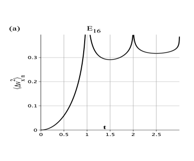
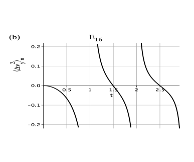
Figure 1: The $x$ and $y$ components [panels (a), left and (b), right)] of the normalized velocity dispersion $\langle{\Delta}\mathbf{v}^{2}(\mathbf{x},t)\rangle_{\,\mbox{n}}$ [Eq. (32)] of a test particle with mass $m$ and charge $q$ in Minkowski space-time with spatial section endowed with the nontrivial $E_{16}$ topology with compact length $a=1$. This figure make apparent that the nontrivial $E_{16}$ topology allows for motion of charged particle under electromagnetic vacuum fluctuations. Clearly, from the topological symmetry the curve for $z$ component is similar to the curves for $y$ component of the velocity dispersion. The divergent behavior of the normalized velocity dispersion components for some values of the time $t$ arises from periodic conditions imposed by $E_{16}$ topology on the covering space $\mathbb{E}^{3}$.

Panels (a) and (b) of Fig. 1 show, respectively, the time behavior of the $x$ and $y$ components of the normalized mean squared velocity fluctuations

$$\langle{\Delta}\mathbf{v}^{2}(\mathbf{x},t)\rangle_{\,\mbox{n}}\equiv(m^{2}/q^{2})\,\langle\Delta\mathbf{v}^{2}\,(\mathbf{x},t)\rangle\,.$$ (32)

In the numerical calculations to plot the curves in both panels of Fig. 1 we have set the compact length $a=1$, and taken $100$ terms of topological contribution to the dispersion, namely $n_{x}\neq 0$ in the interval $[-50,50]$.

From equations (30) and (31) one clearly has divergent behaviors of the normalized velocity dispersion [Eq. (32)], which are shown in both panels of Fig. 1. These divergent behaviors arise from the periodic conditions ($x\rightarrow x^{\prime}=x+n_{x}a$) imposed by $E_{16}$ topology on the covering space. The singular points of the dispersion correspond to $t=n_{x}a\,$ for $\,n_{x}=1,2$ and $3$. The periodicities are given by circles $\mathbb{S}^{1}$, and the singular points correspond to the periods of time required for light to travel, respectively, $\,n_{x}=1,2$ and $3$ times the compact length $a$. For all nontrivial topologies we are concerned with in this paper the covering manifold is infinite and the covering group $\Gamma$ tiles $\mathbb{E}^{3}$ into infinite cells. Therefore, there are infinite singularities of topological origin that arise at certain discrete times $t$ and are associated to periodic conditions imposed by the underlying spatial topology. We briefly indicate below a possible approach to regularize these singularities. In what follows in the figures of the dispersion we exhibit only two (sometimes three or just one) of such singularities, though.

Similar divergent behavior has been reported in the study of the velocity dispersion for the motion of charged particles under electromagnetic fluctuations in Minkowski empty space, whose motions are obtained via what can be looked upon as a change in the spatial topology through the insertion of a plane into the simply-connected $3-$space section of Minkowski $4-$D space-time yf04 ; yc04 . The insertion of a plane along with the rigid perfectly reflecting boundary conditions (method of images BrowMaclay-1969 ) can then be seen as a topological intervention that tiles the covering noncompact $3-$space into two identical domains, and the resulting spatial section is not a manifold, but the nontrivial inhomogeneous quotient orbifold that arises from the action of $\mathbb{Z}_{2}$ on $\mathbb{E}^{3}$ by reflection (see example 13.1.1 in Chapter 13 of Thurston book Thurston ). Thus, the half-space is a quotient space. The motion of the charged particle depends on the particle’s position relative to the plane. The important point is that one can look upon the particles motion as induced by the nontrivial spatial topology, which allows for the motion of test particle under electromagnetic fluctuations in the Minkowski space-time. An important circle $\mathbb{S}^{1}$ in this inhomogeneous $3-$space is defined through the double of this distance from a point to the plane boundary (round-trip). This double-distance plays similar role to that of the compact length $a$ in the Slab topology. But, unlike the case with the Slab topology in which we have infinite singular points, with the insertion of perfectly reflecting plane boundary we have two identical domains with contribution for the dispersion, and with just one singular point for the whole time evolution of the dispersion.

Assuming that the divergence of the velocity dispersion is result of simplified hypothesis about the physical system, local modification through the introduction of a switching function connecting different stages of the system has been suggested to regularize the divergence sw08 ; sw09 ; lrs16 ; lr19 . The ad hoc parameters of the switching functions are thought of as local characteristic of the original system such as width and duration of the switching process, for example. Nevertheless, for the simple topology as $E_{16}$ the compact length $a$ and the time $t$ are equal up to a constant, and thus the proposed switching function can be recast in terms of the topological parameters $a$ (and $n_{x}$) to similarly regularize the divergences taking into account its topological origin. It should be noted that for topologies with higher degree of multiply-connectedness, it is necessary a function of topological parameters, or perhaps several functions, to locally regularize all the divergences of topological origin. This is an issue beyond the scope of the present paper, though.

Returning to Fig. 1 from panel a of one has that the component of dispersion along the compact direction is positive during the whole time evolution. This feature permits the definition of an effective temperature associated to the component of the stochastic motions as in previous works, where plane boundaries have been used yf04 ; yc04 . Panel b on the other hand, exhibits negative dispersions in some interval of time. Negative dispersion has also been reported in previous works with both original yf04 and modified yc04 ; lms14 ; lrs16 system and has been often intrepreted as a consequence of the renormalization with respect to the Minkowski vacuum fluctuations. In Sec. III.1 we have also subtracted the Minkowski vacuum fluctuations term by excluding $n_{x}=0$ from the summation in equation (16), with similar effect in the eletromagnetic correlation function for the Slab and other topologies considered in this paper.

Differently from the motion obtained via the insertion of ad hoc planes into the trivial Minkowski $3-$space yf04 ; yc04 , which breaks its smooth manifold attributes as well as it global spatial homogeneity, here the motion of test particle under vacuum fluctuations takes place in Minkowski space-time whose spatial section is a globally homogeneous smooth manifold $M_{3}$ with $E_{16}$ topology. Furthermore, with insertion of planes the dispersion evolution depends on the position of the test particle relative to the plate. Here, however, since $E_{16}$ is globally homogenous the dynamical behavior of the particles is independent of its position $\mathbf{x}$ on the spatial section of Minkowski space-time.

Two important limiting cases of the above velocity dispersion components (30) and (31) are for $a\gg c\,t$ and for $a\ll c\,t$, where $a$ is the compact length and here $c$ is the speed of light, which has been taken equal to $1$ throughout this paper. The former limit can be obtained either topologically, by increasing the compact length $a$ for a fixed finite period of time, or by fixing a given topological length $a$ (fix a manifold) and restricting locally the time evolution of the particle to a fixed finite small time $t$.

For a sufficiently large compact fixed length $a$, which defines a spatial manifold, and for small time $t$ ($\,t\ll a\,$), from equations (30) – (31) after some simplifying calculations one locally has

$$\langle\Delta v_{x}^{2}\rangle\approx\frac{\pi^{2}q^{2}}{45m^{2}}\frac{t^{2}}{a^{4}}\,,$$ (33)

$$\langle\Delta v_{y}^{2}\rangle=\langle\Delta v_{z}^{2}\rangle\approx-7\times 10^{-2}\frac{q^{2}t^{4}}{m^{2}a^{6}}\,.$$ (34)

Panels (a) and (b) of Fig. 1 also illustrate the different behavior in this limit for small time and signs of the dispersions in $x$ and $y$ (or $z$) directions in this limit. Equations (33) and (34) along with these panels show the absolute values of mean squared velocity fluctuations tends distinctively to zero. The nontrivial topology plays different role even for small time in compact and noncompact directions.

Throughout this paper we shall refer to the limits obtained by increasing the topological length, such as $a\gg t$, as Minkowskian topological limit (or simply Minkowskian limit), in the sense that the role played by the topology when the compact length, $a$, grows tends to that of the simply-connected spatial topology. As the topological compact length tends to infinity the mean squared velocity fluctuations in the noncompact directions $y$ and $z$ decreases to zero faster than the component in the compact direction $x$.

Panels (a) and (b) of Fig. 2 illustrate the topological Minkowskian limit as the compact length takes different values $a=3,6,9$. For these curves the greater is the value of the compact topological length $a$ the longer is the time interval $\Delta t_{\mbox{ng}}$ for which the velocity dispersion is negligible. Thus, in the Minkowskian topological limit $a\rightarrow\infty$ the whole space is simply-connected and $\Delta t_{\mbox{ng}}\rightarrow\infty$, i.e. during the whole time there is no velocity dispersion of the charged particle in Minkowski space-time with simply-connected spatial topology. This outcome agrees with earlier result which claims that in the standard simply-connected Minkowski space-time vacuum quantum fluctuations would not produce stochastic motions of charged particles gs99 ; jr92 . We shall return to the topological Minkowskian limit in the next section where we investigate the motions of test particle in Minkowski space-time with spatial section endowed with topologies with higher degree of connectedness such as Chimney and $3-$Torus spaces, for example.

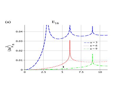
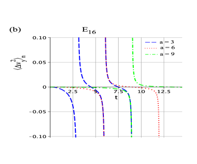
Figure 2: [Panel (a), left]: $x$ and [panel (b), right]: $y$ components of the normalized velocity dispersion $\langle{\Delta}\mathbf{v}^{2}(\mathbf{x},t)\rangle_{\,\mbox{n}}$   [Eq. (32)] of a $q$-charged test particle with mass $m$ in Minkowski space-time with nontrivial $E_{16}$ spatial topology. The curves for manifolds with increasing $a=3,6,9$ are shown to illustrate the topological Minkowskian limit when the compact length $a$ increases. For these curves the greater is the value of the compact topological lengths the longer is the time interval $\Delta t_{\mbox{ng}}$ for which the velocity dispersion of is negligible. In the topological Minkowskian limit $a\rightarrow\infty$ one has $\Delta t_{\mbox{ng}}\rightarrow\infty$, and thus during the whole time there is no motion of a charged particle in Minkowski space-time with simply-connected spatial topology. The topological symmetries of $E_{16}$ topology imply that curves analogous to those for $y$ component hold for the $z$ component of the normalized velocity dispersion.

IV.2 Chimney space – $\mathbf{E_{11}}$

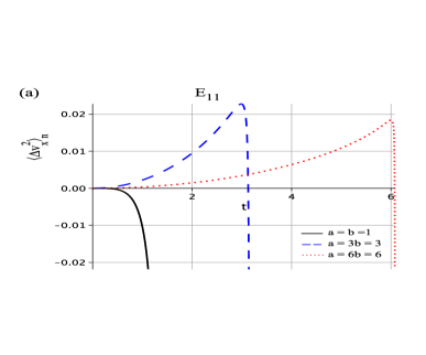
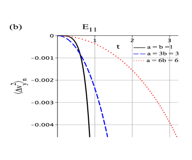
Figure 3: The $x$ and $y$ components [ panels (a) and (b) ] of the normalized velocity dispersion $\langle{\Delta}\mathbf{v}^{2}(\mathbf{x},t)\rangle_{\,\mbox{n}}$   [see Eq. (32)] particle with mass $m$ and charge $q$ in Minkowski space-time whose spatial has the nontrivial Chimney topology $E_{11}$. Curves for manifolds with fixed $b=1$ and three increasing compact lengths $a=1,3,6$ are displayed to illustrate the dispersion in topological Minkowskian limit for $E_{11}$ topology. For these curves the greater is the value of the compact topological lengths the longer is the time interval $\Delta t_{\mbox{ng}}$ for which the velocity dispersion of is negligible. In the topological Minkowskian limit $a\rightarrow\infty$ the whole space is simply-connected, and one has $\Delta t_{\mbox{ng}}\rightarrow\infty$, so during the whole time there is no velocity dispersion of the charged particle in Minkowski space-time with simply-connected spatial topology. From the topological symmetries, $z$ is a noncompact direction with distinct time evolution and separately shown in Fig. 4.

.

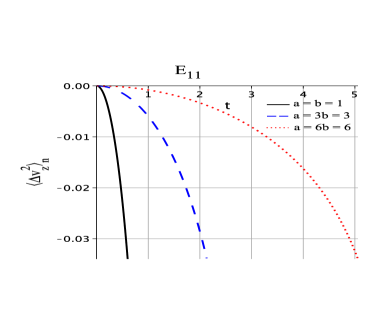
Figure 4: The $z$ component of the normalized velocity dispersion $\langle{\Delta}\mathbf{v}^{2}(\mathbf{x},t)\rangle_{\,\mbox{n}}$  [ Eq. (32)] of a test particle with mass $m$ and charge $q$ in Minkowski space-time whose spatial section has the nontrivial Chimney Euclidean topology $E_{11}$. Curves for manifolds with a fixed $b=1$ and increasing compact lengths $a=1,3,6$, are shown to roughly illustrate the topological Minkowskian limit for $E_{11}$ topology. For these curves the greater is the value of the compact topological lengths the longer is the time interval $\Delta t_{\mbox{ng}}$ for which the velocity dispersion of is negligible. In the topological Minkowskian limit $a\rightarrow\infty$ the whole space becomes simply-connected, and one has $\Delta t_{\mbox{ng}}\rightarrow\infty$, so during the whole time there is no velocity dispersion of the charged particle in Minkowski space-time with simply-connected spatial topology.

Two out of the nine orientable Euclidean three-dimensional topologies have two compact directions. In this section we study in more details the stochastic motions of charged particles in Minkowski space-time whose spatial section has the Chimney space topology $E_{11}$. This $3-$space is globally homogeneous. Thus the elements $\gamma$ of the group $\Gamma$ are translations. The fundamental domain is an open parallelepiped (Chimney), and one identifies the two pairs of faces through independent translations. Taking $x$ and $y$ as the two independent compact directions and $a$ and $b$ as the associated compact lengths, the expression for the spatial separation is then given in the second row of Table 2.

Following a similar procedure to that employed for the Slab topology in the previous section, for the spatial section with Chimney $E_{11}$ topology the electromagnetic field correlation function is given by equation (19) with spatial separation given in Table 2. In the coincidence limit $\mathbf{x}\rightarrow\mathbf{x}^{\prime}$ one has $r^{2}=n_{x}^{2}a^{2}+n_{y}^{2}b^{2}$, $\widetilde{r_{x}}^{2}=-n_{x}^{2}a^{2}+n_{y}^{2}b^{2}$, $\widetilde{r_{y}}^{2}=n_{x}^{2}a^{2}-n_{y}^{2}b^{2}\,$ and $\widetilde{r_{z}}^{2}=n_{x}^{2}a^{2}+n_{y}^{2}b^{2}\,$. The global homogeneity of $E_{11}$ topology implies that $A_{i}=B_{i}=1$ for $i=x,y,z$. Inserting these limiting relations into (III.2) after some simplifying calculation we have that the components of the mean squared velocity dispersion are given by

$$\langle\Delta v_{x}^{2}\rangle=\frac{q^{2}}{2\pi^{2}m^{2}} \sum\limits_{{\!n_{y}=-\infty}}^{{\infty\;\;^{\prime}}}\Biggl{[}\,\,\sum\limits_{{n_{x}=-\infty}}^{{\infty\;\;^{\prime}}}\left\{\frac{t^{2}n_{y}^{2}b^{2}}{(n_{x}^{2}a^{2}+n_{y}^{2}b^{2})^{2}(t^{2}-n_{x}^{2}a^{2}-n_{y}^{2}b^{2})}\Biggr{.}\right.$$

$$\Biggl{.}\left.\qquad+\,\frac{t(-2n_{x}^{2}a^{2}+n_{y}^{2}b^{2})}{4(n_{x}^{2}a^{2}+n_{y}^{2}b^{2})^{5/2}}\,\ln\left(\frac{(\sqrt{n_{x}^{2}a^{2}+n_{y}^{2}b^{2}}-t)^{2}}{(\sqrt{n_{x}^{2}a^{2}+n_{y}^{2}b^{2}}+t)^{2}}\right)\right\}\,\,\,\Biggr{]}\,,$$ (35)

$\langle\Delta v_{y}^{2}\rangle=\langle\Delta v_{x}^{2}\rangle$ with $n_{y}\rightleftarrows n_{x}$ and $b\rightleftarrows a$, and

$$\langle\Delta v_{z}^{2}\rangle=\frac{q^{2}}{2\pi^{2}m^{2}} \sum\limits_{{\!n_{y}=-\infty}}^{{\infty\;\;^{\prime}}}\Biggl{[}\,\,\sum\limits_{{n_{x}=-\infty}}^{{\infty\;\;^{\prime}}}\left\{\frac{t^{2}}{(n_{x}^{2}a^{2}+n_{y}^{2}b^{2})(t^{2}-n_{x}^{2}a^{2}-n_{y}^{2}b^{2})}\Biggr{.}\right.$$

$$\Biggl{.}\left.\qquad\quad+\,\frac{t}{4(n_{x}^{2}a^{2}+n_{y}^{2}b^{2})^{3/2}}\ln\left(\frac{(\sqrt{n_{x}^{2}a^{2}+n_{y}^{2}b^{2}}-t)^{2}}{(\sqrt{n_{x}^{2}a^{2}+n_{y}^{2}b^{2}}+t)^{2}}\right)\,\right\}\,\,\,\Biggr{]}\,.$$ (36)

It should be noticed that only when the $3-$space manifold has equal compact lengths ($a=b$) the associated $x$ and $y$ components of the dispersion have identical behavior. In this case the roles played by the compactness in these directions are equivalent. The velocity dispersion behavior in this specific Chimney manifold corresponds to the solid line curves in Figs. 3 and 4.

From the equation for $\langle\Delta v_{y}^{2}\rangle$ along with Eqs. (IV.2), (IV.2) a first important outcome, which is also made evident in Figs. 3 and 4 and that ratifies previous results with the Slab topology, is that compactification of two independent directions gives rise to stochastic motion of charged particles whose resulting dispersion $\langle\Delta\mathbf{v}^{2}\left(\mathbf{x},t\right)\rangle$ has components not only in the two compact directions but also in the noncompact direction $z$. The solid line curve Figs. (3) and (4) for the spatial manifold with compact lengths $a=b=1$ shows the divergences in the velocity dispersion, which again is of topological origin. The other curves are for different manifolds ($a=3b=3$, $a=6b=6$) also contain topological divergence at $t\simeq 3$ and $t\simeq 6$ not completely displayed in these figures that was produced to illustrate mainly other features of the velocity dispersion.

To examine the topological Minkowskian limit as the compact length $a$ increases we have fixed the value of the compact length $b=1$ and increased $a=1,3,6$, etc. The curves for three manifolds with increasing compact length $a$ are also shown in Figs. 3 and 4. For these curves the greater is the value of the compact topological lengths the longer is the time interval $\Delta t_{\mbox{ng}}$ for which the velocity dispersion of is negligible. Thus, in the Minkowskian topological limit $a\,,b\rightarrow\infty$ the whole space is simply-connected, and one has $\Delta t_{\mbox{ng}}\rightarrow\infty$, i.e. during the whole time there is no velocity dispersion of the charged particle in Minkowski space-time with simply-connected spatial topology. This outcome for Minkowski space-time with Chimney spatial manifolds extends the result of the previous section with the Slab topology, and again it is consistent with an earlier result in the literature that ensures that quantum vacuum fluctuations would not produce stochastic motions of charged particles in Minkowski space-time with simply-connected spatial section.

IV.3 Chimney space with half turn – $\mathbf{E_{12}}$

When the Euclidean distance $d(\mathbf{x},\gamma\mathbf{x})$ between a point $\mathbf{x}\in M_{3}$ and its image $\gamma\mathbf{x}$ is a constant for all points $\mathbf{x}\in M_{3}$, then the holonomy $\gamma$ is a translation. In globally homogeneous quotient manifolds all elements $\gamma$ of the covering group $\Gamma$ are translations. In these manifolds all points $\mathbf{x}$ are topologically indistinguishable. Thus, the effect of the topology in the evolution of a physical system in globally homogeneous manifold is expected to be the same regardless of spatial position in $M_{3}$. This is precisely the case of Slab and Chimney spaces, which have been used in sections IV.1 and IV.2 as spatial section of Minkowski space-time.

In globally inhomogeneous manifolds the distance function $d(\mathbf{x},\gamma\mathbf{x})$ is not constant, and the length of the closed geodesic associated with at least one non-translational $\gamma$ depends on the point $\mathbf{x}\in M_{3}$. In this way, in globally inhomogeneous manifolds the identification of at least one pair of faces of the fundamental domain is made through a combination of a rotation followed by a translation along an axis. The Chimney with half turn of Table 1 is a globally inhomogeneous manifold.

In this section we report the results of our study of the motions of charged test particles in Minkowski space-time whose spatial sections are endowed with the Chimney with half turn topology. Our main goal here is to concretely exhibit the dependency of the velocity dispersion with the particle position in the spatial section endowed with $E_{12}$ topology

Following a similar procedure to that employed in the previous sections IV.1 and IV.2 the electromagnetic field correlation function is given by equation (19) with spatial separation given in Table 2, where $x$ and $y$ were taken as the two independent compact directions and $a$ and $b$ are the associated compact lengths.

Inserting the coincidence limit ($\mathbf{x}\rightarrow\mathbf{x}^{\prime}$) expressions for $r^{2}$, $\widetilde{r_{x}}^{2}$, $\widetilde{r_{y}}^{2}$ and $\widetilde{r_{z}}^{2}$ along with $A_{i}$ and $B_{i}$ ($i=x,y,z$) into (III.2) after simplifying calculations we end up with lengthy expressions for components of the mean squared velocity dispersion, which we do not present here for the sake of conciseness. These expressions were used in the numerical calculations for the plots of the figures in this section.

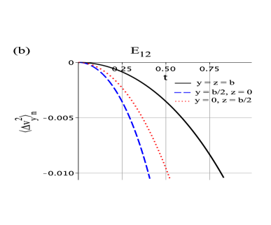
Figure 5: The $x$ and $y$ components [ panels (a)in the left hand side, and (b) in the right ] of the normalized velocity dispersion $\langle{\Delta}\mathbf{v}^{2}(\mathbf{x},t)\rangle_{\,\mbox{n}}$ [Eq. (32)] particle with mass $m$ and charge $q$ in Minkowski space-time whose spatial section has the Euclidean nontrivial $E_{12}$ topology. Curves for a manifold with equal compact length $a=b=1$ are depicted. These curves illustrate that the time-evolution of the velocity dispersion of the charged particle depends upon the particle’s position in the space. In each panel different curves correspond to different particle’s positions in the spatial section of Minkowski space-time. From the topological symmetry $z$ is a noncompact direction with distinct time evolution that is separately exhibited in Fig. 6.

.

Panels (a) and (b) of Fig. 5 along with Fig. 6 show, respectively, the time behavior of $i=x,y,z$ components of the normalized mean squared velocity fluctuations $\langle{\Delta}\mathbf{v}^{2}(\mathbf{x},t)\rangle_{\,\mbox{n}}\equiv(m^{2}/q^{2})\,\langle\Delta\mathbf{v}^{2}\,(\mathbf{x},t)\rangle$ of a test particle with mass $m$ and charge $q$ in Minkowski space-time whose spatial section is a Chimney with half a turn manifold with topological lengths $a=b=1$. In the numerical calculation of each component in Fig. 5 and Fig. 6 we have taken in the summations $100$ terms of the topological contribution to the dispersion, namely $n_{x}\neq 0\,,n_{y}\neq 0$ in the interval $[-50,50]$.

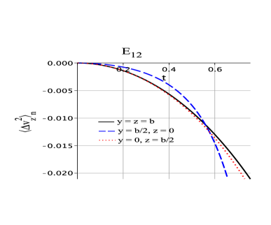
Figure 6: The $z$ components of the normalized velocity dispersion $\langle{\Delta}\mathbf{v}^{2}(\mathbf{x},t)\rangle_{\,\mbox{n}}$ [Eq. (32)] of a test particle with mass $m$ and charge $q$ in Minkowski space-time with spatial section endowed with the nontrivial Euclidean topology $E_{12}$. Curves for a manifold with compact lengths $a=b=1$ are shown. Different curves correspond to different particle’s positions in the spatial manifold. The curves illustrate that the time-evolution of the velocity dispersion of the charged particle depends upon the particle’s position in the spatial section of Minkowski space-time.

Three different spatial positions of the test particle $y=z=b$, $y=b/2,z=0$, and $y=0,z=b/2$ have been taken in order to make evident the distinct time evolution of the normalized dispersions for each particle position. Figures 5 and 6 show the different time behavior of the components of the dispersion, including the divergences for the velocity dispersions that now also depend on the particle position. Preliminary numerical calculations for $E_{12}$ indicate that for the above particle’s positions the curves for the components of the velocity dispersion present, in the Minkowskian limit, similar pattern of the corresponding curves for the other homogeneous manifolds.

An important outcome from these figures is that the time evolution of the dispersion component depends on the test particle position in the spatial section $M_{3}$. In other words, the effect of the topology depends on the spatial position of the test particle. This suggest that the time evolution of a physical system can in principle be used to unveil the global homogeneity or inhomogeneity which are important topological properties of the space-time.

IV.4 $3\,-$Torus  –   $E_{1}$

Possibly the best known example of three-dimensional Euclidean space with nontrivial topology is the $3-$Torus family of globally homogeneous manifolds with three independent compact directions. The manifolds in the $3-$Torus class have therefore higher degree of connectedness than those in the homogeneous Slab ($E_{16}$) and Chimney ($E_{11}$) families which we have considered in the previous sections.

To include an entirely compact Euclidean manifolds in our analysis we have also examined the motions of charged particles in Minkowski space-time in which the spatial section is endowed with the $3-$Torus topology. However, given the previous results concerning the time evolution in Minkowski space-time with the Slab ($E_{16}$) and Chimney ($E_{11}$) spatial topologies, it is expected that the $3-$Torus spatial topology will clearly give rise to stochastic motion of charged test particles. In this way, our main point here is not to verify that these expected motions can indeed occur, but rather to show that the previous outcomes obtained for Chimney, Slab and the simply-connected Minkowskian limit can be recast as appropriate limits in the $3-$Torus spatial topology.

In general, the fundamental cells for $3-$Torus topology can be taken to be a parallelepiped with different compact lengths $a,b,c$, whose faces are identified through independent translations to form the manifolds.

We again follow a procedure similar to that used in sections IV.1, IV.2 and IV.3 but now the electromagnetic field correlation function is given by equation (20) with spatial separation $r$ given by the fourth entry in Table 2, where $x$, $y$ and $z$ are the three independent compact directions, and $a$, $b$ and $c$ are the associated compact lengths. In the coincidence limit $\mathbf{x}\rightarrow\mathbf{x}^{\prime}$ one has the spatial separation reduces to $r^{2}=n_{x}^{2}a^{2}+n_{y}^{2}b^{2}+n_{z}^{2}c^{2}$. The other terms $\widetilde{r_{i}}$ that are needed to have the components of the velocity dispersion (III.2) in the coincidence limit are given by $\widetilde{r_{x}}^{2}=-n_{x}^{2}a^{2}+n_{y}^{2}b^{2}+n_{z}^{2}c^{2}\,$,  $\widetilde{r_{y}}^{2}=n_{x}^{2}a^{2}-n_{y}^{2}b^{2}+n_{z}^{2}c^{2}\,$, and $\widetilde{r_{z}}^{2}=n_{x}^{2}a^{2}+n_{y}^{2}b^{2}-n_{z}^{2}c^{2}$.  As for the constants $A_{i}$ and $B_{i}$ we have $A_{i}=B_{i}=1$ for $i=x,y,z$ from the global homogeneity of the $3-$Torus.

Inserting these coincidence limiting relations into (III.2) after simplifying calculations we end up with lengthy expressions for the components of the velocity dispersion, which we do not present here for conciseness, but that were used in the numerical calculations in the plots of the figures we discuss in what follows.

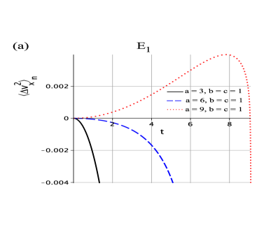
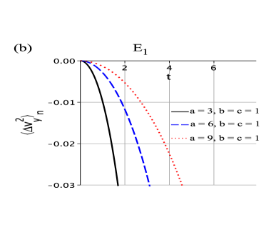
Figure 7: The $x$ and $y$ components [ panels (a) on the left, and (b) on the right hand side ] of the normalized velocity dispersion $\langle{\Delta}\mathbf{v}^{2}(\mathbf{x},t)\rangle_{\,\mbox{n}}\equiv(m^{2}/q^{2})\,\langle\Delta\mathbf{v}^{2}\,(\mathbf{x},t)\rangle$ of a test particle with mass $m$ and charge $q$ in Minkowski space-time whose spatial section has the $3-$Torus topology, $E_{1}$. Curves for manifolds with equal compact length $b=c=1$ and increasing $a=3,6,9$ are shown to illustrate the topological limit for small time $t$.

.

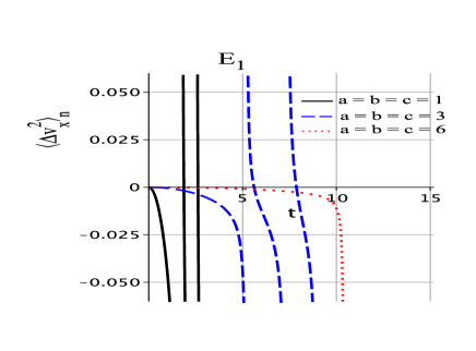
Figure 8: The $x$ component of the normalized velocity dispersion $\langle{\Delta}\mathbf{v}^{2}(\mathbf{x},t)\rangle_{\,\mbox{n}}\equiv(m^{2}/q^{2})\,\langle\Delta\mathbf{v}^{2}\,(\mathbf{x},t)\rangle$ of a test particle with mass $m$ and charge $q$ in Minkowski space-time with spatial has the $3$-Torus topology $E_{1}$. The $y$ and $z$ components time evolution of the normalized dispersion are equal to the $x$ component since $a=b=c$. Curves for manifolds with compact lengths $a=b=c=1,3,6$ are shown. The divergent behavior of the normalized velocity dispersion for some values of the time $t$ arises from periodic conditions imposed by $E_{1}$ topology on the covering space $\mathbb{E}^{3}$. The divergent behavior of the normalized velocity dispersion arises from periodic conditions imposed by the topology.

Panels (a) and (b) of Fig. 7 show, respectively, the time evolution of the $x$ and $y$ components of the normalized dispersion $\langle{\Delta}\mathbf{v}^{2}(\mathbf{x},t)\rangle_{\,\mbox{n}}$ of a charged test particle in Minkowski space-time whose spatial sections are manifolds endowed with a $3-$Torus topology.

To make use of our physical system in the approach to the Chimney space $E_{11}$ as a limiting of $3-$Torus when two topological lengths are fixed and a remaining length increases, we have taken $b=c=1$ and increasing values $a=3,6,9$ in panels a and b of Fig. 7. Clearly for this choice of lengths the $z$ component of the velocity dispersion has the same time evolution of $y$ component, which is exhibited in the panel b. In the numerical calculation of each component in of Figs. 7 and Fig. 8 as in the previous plots we have taken $100$ terms in the summations, i.e. $n_{x}\neq 0\,,n_{y}\neq 0\,,n_{z}\neq 0$ in the interval $[-50,50]$. The divergences in the component of the velocity dispersion in this figures come from the $3$ compactification of the Torus. This was not the main features we illustrate in these figures, though.

The comparison of Fig. 7 with Figs. 3 for the Chimney space make apparent that the evolution of our physical system in Minkowski space-time with Chimney spatial topology $E_{11}$ can be recovered from the evolution of the system in Minkowski with a $3-$Torus topology.

Finally, to the extent that the greater is the value of the compact lengths ($a,b,c$) the longer is the time interval in which the components of the dispersion are negligible, the Fig. 8 indicates that the topological Minkowskian limit can also be obtained from the $3-$Torus when all lengths grow indefinitely, i.e. $(a\,,b\,,c)\rightarrow\infty$. Also compare, for increasing the compact lengths, Fig. 8 with Fig. 3 and then examine Fig. 2 for small time $t$.

V Final Remarks

In the standard approach to model the physical world, besides the points on the space-time manifold representing the physical events, we have fields that satisfy appropriated differential equations, which locally express the physical laws. In the framework of field theories in curved space-times it is often assumed that a geometry, solution of the gravitational field equations, couples to other fields and constrains their dynamics. In this geometric approach the role played by the topology is either implicitly (or explicitly) neglected or left open.

Although they might not be recognized at first sight, topological considerations are sometimes essential in physics (see related Refs. BGRT-1998 ; GRTB-2000 ; MMS-2015 ; RTT-1998 , and references therein quoted). In quantum field theory, which handles, e.g., with field dynamics and its fluctuations on differentiable manifolds, questions as to what extent and how physical outcomes depend upon, are induced, or even driven by a nontrivial topology, are very important.

Quantum vacuum fluctuations of the electromagnetic field in the standard Minkowski space-time with simply-connected spatial section seem not to produce observable effects on the motion of a charged test particle. However, when changes in the background space for the fluctuations are carried out, as for example by the insertion of plane-boundaries into the three-dimensional space, the resulting mean squared velocity of a test charged particle is not null yf04 ; yc04 .

In this article we have tackled the question as to whether a nontrivial spatial topology of Minkowski space-time provides conditions for a charged particle to undergo stochastic motion when subjected to fluctuations of the electromagnetic field in empty space. To answer this question, we have derived the mean squared velocity dispersion of a charged test particle in Minkowski flat space-time whose spatial section has one, two and three independent compact directions. Equations (25) – (III.2) explicitly give the velocity dispersion in these cases with compact spatial orientable topologies. In these equations the spatial separation $r$ takes different forms (Table 2) so as to capture the periodic conditions imposed by the spatial topology. In brief, equations (25) – (III.2) show that quantum vacuum fluctuations in an empty Minkowski space-time with nontrivial spatial topology allow for stochastic motions of charged particles.

To further explore the role played by the spatial topology in the evolution of the velocity dispersion, we have concretely examined the details of the motion of a charged particle for the $3-$spaces endowed with four flat topologies of Table 1, namely three globally homogeneous Slab ($E_{16}$), Chimney ($E_{11}$), $3-$Torus ($E_{1})$, and the globally inhomogeneous Chimney with half a turn ($E_{12}$) topology. A general outcome from the study with these topologies is that compactification in just one direction is sufficient to produce motion of charged particles with velocity dispersion components in the compact and noncompact directions. Here, differently from the motion obtained via the insertion of planes, the motion of a charged particle under vacuum fluctuations in Minkowski space-times occurs with no change of the smooth manifold attributes of the space. Also, for the globally homogeneous spatial topologies $E_{1}$, $E_{11}$ and $E_{16}$ the global spatial homogeneity is unaltered from the outset. In this way, the topological effects on the whole evolution of the velocity dispersion is the same regardless of the particle’s position in the spatial section $M_{3}$.

It is well-known that Minkowski space-time is spatially flat and locally homogeneous. Local homogeneity is a geometrical characteristic of metric manifolds. However, in dealing with topological spaces we have global homogeneity and inhomogeneity of topological nature (Section II). An interesting question that arises in this context is whether a local experiment can be prepared to possibly unveil these global (topological) properties of the space. To illustrate that the motion of a charged particle under vacuum fluctuations can potentially be used to capture or detect global inhomogeneity, we have also examined the motion of charged particle in Minkowski space-time with $E_{12}$ spatial globally inhomogeneous topology. Figures 5 and 6 show that different spatial position $\mathbf{x}$ of the particle leads to different curves for the velocity dispersion. Hence, the time evolution of the velocity dispersion for a charged particle under electromagnetic fluctuations can be locally used to unveil the global inhomogeneity of the space.

It seems to be unsettled whether electromagnetic quantum vacuum fluctuations in standard Minkowski space-time with simply-connected spatial section would allow for motion of a charged test particle. This would be an observable effect of vacuum fluctuations. In this paper we have also tackled this issue by considering the topological Mikowskian limit, in which the infinite spatial manifold with simply-connected topology can be obtained from globally homogeneous manifolds through limit when the compact topological lengths grow indefinitely. We have found that, regardless the globally homogeneous topology we start from (seed manifold), the greater is the value of the topological length the longer is the time interval $\Delta t_{\mbox{ng}}$ for which the velocity dispersion is negligible. In the limit when the topological lengths $(a\,,b\,,c)$ tend to infinite, the time interval $\Delta t_{\mbox{ng}}$ in which the dispersion is negligible also tends to infinite, $\Delta t_{\mbox{ng}}\rightarrow\infty$. Thus during the whole time there is no motion of a charged particle in Minkowski space-time with simply-connected spatial topology. In Fig. 2, for example, we illustrate this topological limit for small time $t$, increasing compact length $a$ and for manifolds with the Slab spatial topology $E_{16}$. This result holds for Mikowskian limits of other manifolds with homogeneous topologies $E_{11}$ and $E_{1}$ (Figs. 3, 4 and 7 and  8). These topological Minkowskian limit results make apparent that no motion of a charged particle arises from quantum electromagnetic fluctuations in the standard Minkowski space-time with simply-connected spatial section. The ultimate motive behind the stochastic motion of a charged particle under electromagnetic quantum vacuum fluctuations is the nontrivial space topology.

- (1) G.F.R. Ellis, Gen. Rel. Grav. 2, 7 (1971); M. Lachièze-Rey and J.P. Luminet, Phys. Rep. 254, 135 (1995); G.D. Starkman, Class. Quantum Grav. 15, 2529 (1998); J. Levin, Phys. Rep. 365, 251 (2002); M.J. Rebouças and G.I. Gomero, Braz. J. Phys. 34, 1358 (2004); M.J. Rebouças, A Brief Introduction to Cosmic Topology, in Proc. XIth Brazilian School of Cosmology and Gravitation, eds. M. Novello and S.E. Perez Bergliaffa (Americal Institute of Physics, Melville, New York, 2005) AIP Conference Proceedings vol. 782, p 188, also: arXiv:astro-ph/0504365; J.P. Luminet, Universe 2016, 2(1), 1.
- (2) M.J. Rebouças, Detecting cosmic topology with primordial gravitational waves, in preparation (2020).
- (3) B.P. Abbott et al., Phys. Rev. Lett. 116, 061102 (2016).
- (4) G.I. Gomero, M.J. Rebouças, and R. Tavakol, Class. Quantum Grav. 18, 4461 (2001); G.I. Gomero, M.J. Rebouças, and Reza K. Tavakol, Class. Quant. Grav. 18, L145 (2001); G.I. Gomero, M.J. Rebouças, and R. Tavakol, Class. Quantum Grav. 18, L145 (2001); G.I. Gomero, M.J. Rebouças, and R. Tavakol, Int. J. Mod. Phys. A 17, 4261 (2002); J. Weeks, Mod. Phys. Lett. A 18, 2099 (2003); B. Mota, M.J. Rebouças, and R. Tavakol, Class. Quantum Grav. 20, 4837 (2003).
- (5) P.M. Vaudrevange, G.D. Starkman, N.J. Cornish, and D.N. Spergel, Phys. Rev. D 86, 083526 (2012).
- (6) P.A.R. Ade et al. (Planck Collaboration 2015), Astron. Astrophys. 594, A18 (2016).
- (7) G. Gomero, B. Mota, and M.J. Rebouças, Phys. Rev. D 94, 043501 (2016).
- (8) J.A. Wolf, Spaces of Constant Curvature, McGraw-Hill, New York (1967).
- (9) W.P. Thurston, Three-Dimensional Geometry and Topology. Vol.1, Edited by Silvio Levy, Princeton University Press (1997).
- (10) B.S. DeWitt, C.F. Hart and C.J. Isham, Physica 96A, 197 (1979).
- (11) J.S. Dowker and R. Critchley, J. Phys. A 9, 535 (1976).
- (12) P.M. Sutter and T. Tanaka, Phys. Rev. D 74, 024023 (2006).
- (13) M.P. Lima and D. Muller, Class. Quant. Grav. 24, 897 (2007).
- (14) D. Muller, H.V. Fagundes, and R. Opher, Phys. Rev. D 66, 083507 (2002).
- (15) D. Muller, H.V. Fagundes, and R. Opher, Phys. Rev. D 63, 123508 (2001)
- (16) G. Gour and L. Sriramkumar, Found. Phys. 29, 1917 (1999).
- (17) M.T. Jaekel and S. Reynaud, Quant. Opt. 4, 39 (1992).
- (18) H. Yu and L.H. Ford, Phys. Rev. D 70, 065009 (2004).
- (19) H. Yu and J. Chen, Phys. Rev. D70, 125006 (2004).
- (20) L.H. Ford, Int. J. Theor. Phys. 44, 1753 (2005).
- (21) H.W. Yu, J. Chen, and P. X. Wu, JHEP 0602, 058 (2006).
- (22) J.T. Hsiang, T. H. Wu, and D.S. Lee, Phys. Rev. D 77, 105021 (2008).
- (23) M. Seriu and C.H. Wu, Phys. Rev. A 77, 022107 (2008).
- (24) M. Seriu and C.H. Wu, Phys. Rev. A 80, 052101 (2009).
- (25) V. Parkinson and L.H. Ford, Phys. Rev. A 84, 06210 (2011).
- (26) T.H. Wu, J.T. Hsiang, and D.S. Lee, Annals Phys. 327, 522 (2012).
- (27) C.H. Wu, K.I. Kuo, and L.H. Ford, Phys. Rev. A 65, 062102 (2002).
- (28) C.H.G. Bessa, V.B. Bezerra, and L.H. Ford, J. Math. Phys. 50, 062501 (2009).
- (29) C.H.G. Bessa, V.B. Bezerra, E.R. Bezerra de Mello, and H.F. Mota, Phys. Rev. D 95, 085020 (2017).
- (30) V.A. De Lorenci, E.S. Moreira Jr., and M.M. Silva, Phys. Rev. D 90, 027702 (2014).
- (31) V.A. De Lorenci, C.C.H. Ribeiro, and M.M. Silva, Phys. Rev. D 94, 105017 (2016).
- (32) E. Feodoroff, Russ. J. Crystallogr. Mineral. 21, 1 (1885).
- (33) L. Bieberbach, Math. Ann. 70, 297 (1911).
- (34) L. Bieberbach, Math. Ann. 72, 400 (1912).
- (35) W. Novacki, Comment. Math. Helv. 7, 81 (1934).
- (36) C. Adams and J. Shapiro, American Scientist 89, 443 (2001).
- (37) B. Cipra, What’s Happening in the Mathematical Sciences, American Mathematical Society, Providence, RI, 2002.
- (38) A. Riazuelo, J. Weeks, J.P. Uzan, R. Lehoucq, and J.P. Luminet, Phys. Rev. D 69, 103518 (2004).
- (39) H. Fujii and Y. Yoshii, Astron. Astrophys. 529, A121 (2011).
- (40) N.D. Birrel and P.C.W. Davies, Quantum Fields in Curved Space (Cambridge University Press, Cambridge, England) (1982).
- (41) V.A. De Lorenci, and C.C.H. Ribeiro, 2019 JHEP 04 072
- (42) A. Bernui, G.I. Gomero, M.J. Rebouças, and A.F.F. Teixeira Phys. Rev. D 57, 4699 (1998).
- (43) G.I. Gomero, M.J. Rebouças, A.F.F. Teixeira, and A. Bernui, Int. J. Mod. Phys. A 15, 4141 (2000).
- (44) A. Matas, D. Müller, and G. Starkman, Phys. Rev. D 92 026005 (2015).
- (45) A. Terras, Harmonic Analysis on Symmetric Spaces — Euclidean Space, the Sphere and Poincaré Half-Plane, 2nd ed. (Spriger, New York, 2013.
- (46) L.S Brown and G.J. Maclay, Phys. Rev. 184, 1272 (1969).
- (47) M.J. Rebouças, R.K. Tavakol, and A.F.F. Teixeira, Gen. Rel. Grav. 30, 535 (1998).