Bu, Simchi-Levi, and Xu

Online Pricing with Offline Data

Online Pricing with Offline Data:
Phase Transition and Inverse Square Law

Jinzhi Bu Department of Logistics and Maritime Studies, Faculty of Business, The Hong Kong Polytechnic University, Hung Hom, Kowloon, Hong Kong, jinzhi.bu@polyu.edu.hk David Simchi-Levi Institute for Data, Systems, and Society, Massachusetts Institute of Technology, Cambridge, MA 02139, dslevi@mit.edu Yunzong Xu Institute for Data, Systems, and Society, Massachusetts Institute of Technology, Cambridge, MA 02139, yxu@mit.edu

This paper investigates the impact of pre-existing offline data on online learning, in the context of dynamic pricing. We study a single-product dynamic pricing problem over a selling horizon of $T$ periods. The demand in each period is determined by the price of the product according to a linear demand model with unknown parameters. We assume that before the start of the selling horizon, the seller already has some pre-existing offline data. The offline data set contains $n$ samples, each of which is an input-output pair consisting of a historical price and an associated demand observation. The seller wants to utilize both the pre-existing offline data and the sequentially-revealed online data to minimize the regret of the online learning process.

We characterize the joint effect of the size, location and dispersion of the offline data on the optimal regret of the online learning process. Specifically, the size, location and dispersion of the offline data are measured by the number of historical samples $n$, the distance between the average historical price and the optimal price $\delta$, and the standard deviation of the historical prices $\sigma$, respectively. For the single-historical-price setting where the $n$ historical prices are identical, we prove that the best achievable regret is $\widetilde{\Theta}\left(\sqrt{T}\wedge\frac{T\log T}{(n\wedge T)\delta^{2}}\right)$. For the (more general) multiple-historical-price setting where the historical prices can be different, we show that the best achievable regret is $\widetilde{\Theta}\left(\sqrt{T}\wedge\frac{T\log T}{n\sigma^{2}+(n\wedge T)\delta^{2}}\right)$. For both settings, we design a learning algorithm based on the “Optimism in the Face of Uncertainty” principle, which strikes a balance between exploration and exploitation, and achieves the optimal regret up to a logarithmic factor. Our results reveal surprising transformations of the optimal regret rate with respect to the size of the offline data, which we refer to as phase transitions. In addition, our results demonstrate that the location and dispersion of the offline data also have an intrinsic effect on the optimal regret, and we quantify this effect via the inverse-square law. dynamic pricing, online learning, offline data, phase transition, inverse-square law

1 Introduction

Classical statistical learning theory distinguishes between offline learning and online learning. Offline learning deals with the problem of finding a predictive function based on the entire training data set. The performance of an offline learning algorithm is typically measured by its generalization error (also known as the out-of-sample error) or sample complexity (see, e.g., Hastie et al. 2005). In contrast to the offline learning setting where the entire training data set is directly available before the offline learning algorithm is applied, online learning deals with a setting where data become available in a sequential manner that may depend on the actions taken by the online learning algorithm. The performance of online learning algorithms is typically measured by the regret. While offline learning assumes access to offline data (but not online data) and online learning assumes access to online data (but not offline data), in reality, a broad class of real-world problems incorporate both aspects: there is an offline historical data set (based on historical actions) at the time that the learner starts an online learning process.

Currently, there is no standard framework for the above type of learning problems, as classical offline learning theory and online learning theory have different settings and goals. While establishing a framework that bridges all aspects of offline learning and online learning is generally a very complicated task, in this paper, we propose a framework that bridges the gap between offline learning and online learning in a specific problem setting, which, however, already captures the essence of many dynamic pricing problems that sellers face in practice.

1.1 The Model: Online Pricing with Offline Data

In this paper, we study the Online Pricing with Offline Data (OPOD) problem. Consider a firm selling a single product with an infinite amount of inventory over a selling horizon of $T$ periods. In each period $t=1,2,\ldots,T$, the seller chooses a price $p_{t}$ from a given interval $[l,u]\subset[0,\infty)$ to offer to its customers, and then observes random demand $D_{t}$. We assume that the demand in each period is a linear function of the price plus some random noise. Specifically, for each $t\geq 1$,

$$D_{t}=\alpha^{*}+\beta^{*}p_{t}+\varepsilon_{t},$$ (1)

where $\alpha^{*}$ and $\beta^{*}$ are two unknown demand parameters in the known interval $[\alpha_{\min},\alpha_{\max}]\subseteq(0,\infty)$ and $[\beta_{\min},\beta_{\max}]\subseteq(-\infty,0)$ respectively, and $\{\varepsilon_{t}\}_{t=1}^{T}$ are i.i.d. random variables with zero mean and unknown distribution. We assume that $\varepsilon_{t}$ is an $R^{2}$-sub-Gaussian random variable, i.e., there exists a constant $R>0$ such that $\mathbb{E}[e^{x\varepsilon_{t}}]\leq e^{\frac{x^{2}R^{2}}{2}}$ for any $x\in\mathbb{R}$. For notational convenience, let $\theta^{*}:=(\alpha^{*},\beta^{*})$ and $\Theta^{{\dagger}}:=[\alpha_{\min},\alpha_{\max}]\times[\beta_{\min},\beta_{\max}]$, and we use $\theta:=(\alpha,\beta)$ to denote any possible vector in parameter space $\Theta^{{\dagger}}$.

The seller’s single-period expected revenue is the price $p$ offered to the customer multiplied by the associated expected demand. To emphasize the dependence on the parameter values, for any $\theta=(\alpha,\beta)\in\Theta^{{\dagger}}$, we define the expected revenue function $r(p;\theta)$ as $r(p;\theta)=p(\alpha+\beta p),\,\,\forall p\in[l,u]$. Let $\psi(\theta)$ be the price that maximizes $r(p;\theta)$ over the interval $[l,u]$, i.e., $\psi(\theta)=\arg\max\big{\{}r(p;\theta):p\in[l,u]\big{\}}$, and use $p^{*}$ to denote the true optimal price, i.e., $p^{*}=\psi(\theta^{*})$. Let $r^{*}(\theta)$ be the optimal expected revenue under demand parameter $\theta$, i.e., $r^{*}(\theta)=\psi(\theta)(\alpha+\beta\psi(\theta))$. Without loss of generality, we assume that for any $\theta\in\Theta^{{\dagger}}$, the optimal price is an interior point of price range $[l,u]$, and therefore $\psi(\theta)=\frac{\alpha}{-2\beta}$.

Historical prices and offline data. In reality, the seller does not know the true demand model, but has to learn such information from the historical data. In this paper, we assume that the seller has some pre-existing offline data before the start of the online learning process. The offline data set contains $n$ independent samples: $\{(\hat{p}_{1},\hat{D}_{1}),(\hat{p}_{2},\hat{D}_{2}),\ldots,(\hat{p}_{n},\hat{D}_{n})\}$, where $\hat{p}_{1},\hat{p}_{2},\ldots,\hat{p}_{n}$ are $n$ fixed prices, and each $\hat{D}_{i}$ is a demand observation under historical price $\hat{p}_{i}$, drawn independently according to the underlying linear demand model (1). Therefore, for each $1\leq i\leq n$, $\hat{D}_{i}=\alpha^{*}+\beta^{*}\hat{p}_{i}+\hat{\varepsilon}_{i}$ for some i.i.d. random variables $\{\hat{\varepsilon}_{i}\}_{i=1}^{n}$ with the same distribution as that of $\{\varepsilon_{t}\}_{t=1}^{T}$.

Pricing policies and performance metrics. For each $t\geq 0$, let $H_{t}$ be the vector of information available at the beginning of period $t+1$, i.e., $H_{t}=(\hat{p}_{1},\hat{D}_{1},\ldots,\hat{p}_{n},\hat{D}_{n},p_{1},D_{1},\ldots,p_{t},D_{t})$. A pricing policy is defined as a sequence of functions $\pi=(\pi_{1},\pi_{2},\ldots)$, where each $\pi_{t}$ is a measurable function which maps the realization of $H_{t}$ (and possibly some external randomness) to a feasible price in $[l,u]$. Let $\Pi$ be the set of all pricing policies. For any policy $\pi\in\Pi$, the regret of $\pi$, denoted by $R^{\pi}_{\theta^{*}}(T)$, is defined as the difference between the optimal expected revenue generated by the clairvoyant policy that knows the exact value of $\theta^{*}$ and the expected revenue generated by pricing policy $\pi$, i.e.,

$$R^{\pi}_{\theta^{*}}(T)=T\cdot r^{*}(\theta^{*})-\mathbb{E}^{\pi}_{\theta^{*}}\Big{[}\sum_{t=1}^{T}r(p_{t};\theta^{*})\Big{]},$$

1.2 Research Question, Observations and Challenges

This paper is inspired by the objective of bridging the gap between offline learning and online learning. The following question naturally arises whenever the offline data are incorporated into the online decision making: how do the offline data affect the statistical complexity of online learning? To address this question, the first challenge is to identify the key characteristics of the offline data that intrinsically affect the complexity of the online learning task.

Intuitively, the size of the offline data, measured by the number of historical samples $n$, and the dispersion of the offline data, measured by the standard deviation of historical prices $\sigma$, i.e., $\sigma=\sqrt{\sum_{i=1}^{n}(\hat{p}_{i}-\frac{1}{n}\sum_{j=1}^{n}\hat{p}_{j})^{2}}$, provide two important metrics that enable quantifying the amount of information collected before the online learning process starts. As $n$ becomes larger, or $\sigma$ increases, the seller can form a better estimation for the unknown demand parameters using offline regression, and the regret may decrease accordingly.

Another crucial, and more intriguing metric of the offline data, is the location of the offline data, which is measured by $\delta=|\frac{1}{n}\sum_{i=1}^{n}\hat{p}_{i}-p^{*}|$, i.e., the distance between the average historical price and the optimal price $p^{*}$. We refer to $\delta$ as the generalized distance, as it intuitively quantifies how far the offline data set is “away” from the (unknown) optimal decision. This is a crucial metric that uniquely appears when offline data are incorporated into the online learning process. Indeed, if there are no offline data available before the start of the online learning process, then there is no $\delta$ at all. Also, if the offline data are only used for estimation or prediction, with no need of online decision making, i.e., the seller is purely interested in estimating the model parameters from the offline data and does not need to make any online pricing decisions, then $\delta$ does not affect her estimation accuracy. Surprisingly, as we prove in this paper, when the offline data are incorporated into online learning, this metric will play a fundamental role.

Besides identifying the above three characteristics of the offline data, a key challenge is to precisely quantify the effects of these offline data characteristics on the online learning task. Specifically, we seek to understand to what extent these three metrics of the offline data influence the behavior and growth rate of the best-achievable regret bound. On the algorithmic side, we also seek to design a simple, intuitive and easy-to-implement pricing policy that exploits the values of both the pre-existing offline data and sequentially-revealed online data, and achieves a tight regret bound with respect to the selling horizon $T$, as well as the three metrics of the offline data, i.e., $n$, $\sigma$, $\delta$. Moreover, since the generalized distance $\delta$ is completely unknown to the seller, the algorithm itself cannot use any information about $\delta$, which implies a more challenging task of designing a learning algorithm whose performance is as good as if $\delta$ were known.

1.3 Main Results and Technical Highlights

In this paper, we address the above challenges in two settings: (i) single-historical-price setting where all the historical prices are identical, i.e., $\sigma=0$, and (ii) multiple-historical-price setting where the historical prices can be different, i.e., $\sigma>0$. We next summarize our main results and technical highlights. Throughout this paper, we use $\widetilde{\mathcal{O}}(\cdot)$ and $\widetilde{\Omega}(\cdot)$ to present upper and lower bounds on the growth rate up to logarithmic factors, and $\widetilde{\Theta}(\cdot)$ to characterize the rate when the upper and lower bounds match (up to logarithmic factors). In addition, we use $A\lesssim B$ and $A\gtrsim B$ to denote $A=\widetilde{\mathcal{O}}(B)$ and $A=\widetilde{\Omega}(B)$ respectively. More formal definitions of these notations are provided in §1.5. For any $a,b\in\mathbb{R}$, $a\wedge b=\min\{a,b\}$ and $a\vee b=\max\{a,b\}$.

Single-historical-price setting. For the single-historical-price setting, we develop a learning algorithm called Online and Offline–OFU (O3FU) algorithm, where OFU refers to the principle of Optimism in the Face of Uncertainty, which arises from multi-armed bandits and is widely used in the literature on bandits (see, e.g., Dani et al. 2008, Abbasi-Yadkori et al. 2011). In general, this principle suggests taking actions based on an optimistic guess of the reward associated with each action in each period. We show that the regret of O3FU algorithm has an upper bound $\widetilde{\mathcal{O}}\big{(}\sqrt{T}\wedge\frac{T\log T}{(n\wedge T)\delta^{2}}\big{)}$. Although this upper bound depends on the unknown quantity $\delta$, the algorithm itself does not require any information about $\delta$. In addition, we prove an information-theoretic lower bound which matches the upper bound, showing that the regret bound cannot be further improved by other algorithms (in a certain sense); we define such an unimprovable regret bound as the optimal (instance-dependent) regret for the OPOD problem in the single-historical-price setting. We summarize its rate in Table 1. In particular, when $n=0$, or $n=\infty$ and $\delta$ is a constant independent of $T$, the results in the leftmost and rightmost cases with $\delta\gtrsim T^{-1/4}$ in Table 1 recover those in Keskin and Zeevi (2014).

Multiple-historical-price setting. For the general setting that the historical prices may be different, we modify O3FU algorithm by adding a preliminary step that detects whether a corner case $\delta^{2}\lesssim\frac{1}{n\sigma^{2}}\lesssim\frac{1}{\sqrt{T}}$ happens or not, and propose the Modified O3FU (M-O3FU) algorithm. We prove that M-O3FU algorithm achieves the regret upper bound $\widetilde{\mathcal{O}}(\sqrt{T}\wedge\frac{T\log T}{n\sigma^{2}+(n\wedge T)\delta^{2}})$, except for a corner case where the upper bound becomes $\widetilde{\mathcal{O}}(T\delta^{2})$. In addition, we prove an information-theoretic lower bound that matches the upper bound for both cases, showing that our regret bound cannot be further improved (in a certain sense); we define such an unimprovable regret bound as the optimal (instance-dependent) regret for the OPOD problem in the multiple-historical-price setting. We summarize its rate in Table 2.

Sufficient condition for self-exploration. As a byproduct, we provide a sufficient condition for the myopic (i.e., greedy) policy to self-explore in the online learning process. Specifically, if the variance of historical prices is sufficiently large, and the average historical price is found to be bounded away from the confidence interval for the optimal price constructed from offline regression, then the myopic policy, the one that always charges the optimal price associated with the least-square estimate obtained in each round, achieves the optimal regret under mild conditions. This result generates additional insights for the performance guarantee of the myopic policy with the help of offline data, and also provides analytical support for the wide use of such policies in practice.

Methodology contributions. From a technical perspective, the tight upper and lower bounds that we obtain in this paper are both instance-dependent regret bounds, which are much stronger and more challenging to prove than the traditional worst-case regret bounds. To prove the instance-dependent upper bound, we conduct a period-by-period trajectory analysis, and develop novel inductive arguments, integrated with the specific property guaranteed by OFU principle, to obtain a sharp characterization on the distance between the algorithm’s price and the average historical price. To prove the instance-dependent lower bound, we reduce the OPOD problem to a hybrid of estimation and hypothesis testing problems, which requires constructing an instance-dependent prior distribution and an instance-dependent hypothesis set, respectively. To the best of our knowledge, these are the first tight and general instance-dependent regret bounds obtained in (i) the linear-demand online pricing problem, and (ii) a continuous-armed bandit problem where the optimal action may not be an extremal point (in contrast to the extremal-point requirement in Dani et al. 2008 and Abbasi-Yadkori et al. 2011).

1.4 Key Insights: Phase Transitions and Inverse-Square Law

The characterization of the optimal instance-dependent regret also leads to two important implications on the value of offline data. First, when the offline sample size $n$ changes, the optimal regret rate exhibits significantly different decaying patterns, and we refer to such significant transitions between the regret-decaying patterns as phase transitions. For example, when $\sigma=0$ and $\delta\gtrsim T^{-\frac{1}{4}}$ (see Table 1), the optimal regret rate remains at the level of $\widetilde{\Theta}(\sqrt{T})$ whenever $n\lesssim\frac{\sqrt{T}}{\delta^{2}}$, and then gradually decays according to $\widetilde{\Theta}(\frac{T}{n\delta^{2}})$ when $\frac{\sqrt{T}}{\delta^{2}}\lesssim n\lesssim T$, and finally stays at the level of $\widetilde{\Theta}(\frac{\log T}{\delta^{2}})$ when $n\gtrsim T$. Second, in the regular case, the optimal regret is inversely proportional to the square of the standard deviation $\sigma$ and generalized distance $\delta$, which is referred to as the inverse-square law. The optimal regret’s dependence on $\sigma$ is consistent with our intuition, as more dispersive historical prices indicate more information gained before the online learning process starts, and therefore a smaller regret. The optimal regret’s dependence on $\delta$ is more intriguing, as it suggests that the closer the historical prices are to the optimal price, the worse the optimal regret will be. In fact, this is a consequence of the tradeoff between exploration (i.e., experimenting to improve estimates of the unknown demand model) and exploitation (i.e., leveraging current estimates to maximize revenue). Specifically, whenever an algorithm tries to learn the true demand model, it has to make substantial efforts in charging various prices “far away” from the average historical price. Therefore, when $\delta$ is small, such a deviation will also lead to a significant gap with the optimal price, leading to greater revenue loss. These two findings contribute new insights to the fundamental problem of dynamic pricing with demand learning.

Table 1: Optimal regret for the single-historical-price setting

$\delta\gtrsim T^{-\frac{1}{4}}$
offline sample size	$0\leq n\lesssim\frac{\sqrt{T}}{\delta^{2}}$	$\frac{\sqrt{T}}{\delta^{2}}\lesssim n\lesssim T$	$n\gtrsim T$
optimal regret	$\widetilde{\Theta}(\sqrt{T})$	$\widetilde{\Theta}(\frac{T}{n\delta^{2}})$	$\widetilde{\Theta}(\frac{\log T}{\delta^{2}})$
$\delta\lesssim T^{-\frac{1}{4}}$
offline sample size	$n\geq 0$
optimal regret	$\widetilde{\Theta}(\sqrt{T})$

Table 2: Optimal regret for the multiple-historical-price setting

$\delta\gtrsim T^{-\frac{1}{4}}$ and $\sigma\lesssim\delta$
offline sample size	$0\leq n\lesssim\frac{\sqrt{T}}{\delta^{2}}$	$\frac{\sqrt{T}}{\delta^{2}}\lesssim n\lesssim T$	$T\lesssim n\lesssim\frac{T\delta^{2}}{\sigma^{2}}$	$n\gtrsim\frac{T\delta^{2}}{\sigma^{2}}$
optimal regret	$\widetilde{\Theta}(\sqrt{T})$	$\widetilde{\Theta}(\frac{T}{n\delta^{2}})$	$\widetilde{\Theta}(\frac{1}{\delta^{2}})$	$\widetilde{\Theta}(\frac{T}{n\sigma^{2}})$
$\delta\gtrsim T^{-\frac{1}{4}}$ and $\sigma\gtrsim\delta$
offline sample size	$0\leq n\lesssim\frac{\sqrt{T}}{\sigma^{2}}$		$n\gtrsim\frac{\sqrt{T}}{\sigma^{2}}$
optimal regret	$\widetilde{\Theta}(\sqrt{T})$		$\widetilde{\Theta}(\frac{T}{n\sigma^{2}})$
$\delta\lesssim T^{-\frac{1}{4}}$
offline sample size	$0\leq n\lesssim\frac{\sqrt{T}}{\sigma^{2}}$		$\frac{\sqrt{T}}{\sigma^{2}}\lesssim n\lesssim\frac{1}{\delta^{2}\sigma^{2}}$	$n\gtrsim\frac{1}{\delta^{2}\sigma^{2}}$
optimal regret	$\widetilde{\Theta}(\sqrt{T})$		$\widetilde{\Theta}(T\delta^{2})$	$\widetilde{\Theta}(\frac{T}{n\sigma^{2}})$

1.5 Structure and Notations

This paper is organized as follows. In §2, we review the relevant literature. In §3 and §4, we study the OPOD problem in the single-historical-price setting and multiple-historical-price setting respectively. We conduct a numerical study in §5, and discuss the self-exploration of the myopic policy in §6. In §7, we summarize our paper with extensions and future research directions. Most of the technical proofs are deferred to the appendix.

Throughout the paper, all the vectors are column vectors unless otherwise specified. For any $m\in\mathbb{N}$, we use $[m]$ to denote the set $\{1,2,\ldots,m\}$. For any column vector $x\in\mathbb{R}^{n}$ and positive semi-definite matrix $A\in\mathbb{R}^{n\times n}$, $||x||:=(\sum_{i=1}^{n}x_{i}^{2})^{\frac{1}{2}}$, and $||x||_{A}:=\sqrt{x^{\top}Ax}$. The notations $\mathcal{O}(\cdot)$, $\Omega(\cdot)$ and $\Theta(\cdot)$ are applied to hide constant factors, and $\widetilde{\mathcal{O}}(\cdot)$, $\widetilde{\Omega}(\cdot)$ and $\widetilde{\Theta}(\cdot)$ are applied to hide both constant and logarithmic factors. That is, $f(T)=\mathcal{O}(g(T))$ means that there exists a constant $C>0$ such that $f(T)\leq Cg(T)$ for any $T$, and $f(T)=\widetilde{\mathcal{O}}(g(T))$ means that there exist constants $C$ and $\lambda>0$, such that $f(T)\leq Cg(T)(\log T)^{\lambda}$ for any $T$. In addition, $f(T)=\Omega(g(T))$ (resp. $f(T)=\widetilde{\Omega}(g(T))$) means $g(T)={\mathcal{O}}(f(T))$ (resp. $g(T)=\widetilde{\mathcal{O}}(f(T))$), and $f(T)=\Theta(g(T))$ (resp. $f(T)=\widetilde{\Theta}(g(T))$) means $f(T)=\mathcal{O}(g(T))$ and $f(T)=\Omega(g(T))$ (resp. $f(T)=\widetilde{\mathcal{O}}(g(T))$ and $f(T)=\widetilde{\Omega}(g(T))$).

2 Related Literature

2.1 Dynamic Pricing with Online Learning

When there are no offline data, the OPOD problem becomes a pure online learning problem, i.e. dynamic pricing with an unknown linear demand model, and belongs to a broad category referred to as the online pricing problems. Online pricing problems have generated great interest in recent years in the operations research and management science (OR/MS) community, see den Boer (2015) for a comprehensive survey. In particular, there is a vast literature (e.g., den Boer and Zwart 2013, den Boer 2014, Keskin and Zeevi 2014, Wang et al. 2014, Keskin and Zeevi 2016, Qiang and Bayati 2016, den Boer and Keskin 2017, Nambiar et al. 2019, Ban and Keskin 2020) studying dynamic pricing problems with an unknown linear (or generalized linear) demand model, which is arguably one of the most fundamental demand models for pricing. All of the existing papers purely focus on online learning. In this paper, we take the fundamental problem of dynamic pricing with a linear demand model as our baseline, but significantly extend it by incorporating offline data into online decision making.

Keskin and Zeevi (2014) is the most relevant paper to this work. The authors consider dynamic pricing with an unknown linear demand model, studying an important question of how knowing an exact point at the demand curve (i.e., the exact expected demand under a single price) in advance helps reduce the optimal regret. Depending on whether the seller knows this exact point or not, they prove that the best achievable regret is $\Theta(\log T)$ and $\widetilde{\Theta}(\sqrt{T})$ respectively. Compared with their work, the OPOD problem studied in this paper seems more relevant to practice, and is more general in theory. Practically, while firms will never know the true expected demand under a given price exactly (which requires infinitely many demand observations), they usually have some pre-existing offline data (which are finitely many) prior to the online learning process. Theoretically, the results in Keskin and Zeevi (2014) (for the single-product setting) can be viewed as two special cases of our results when (i) $n=0$; and (ii) $\sigma=0$, $n=\infty$, and $\delta=\Theta(1)$, with an additional assumption that $\delta$ is lower bounded by a known constant (as their algorithms for case (ii) rely on this knowledge). Since $\delta$ is completely unknown and can be small in our setting (and in reality), their algorithms and analysis do not apply here. In fact, the principle of our algorithm design and the approach of our regret analysis are very different from theirs.

There is also a stream of literature in Bayesian learning, where the decision maker is assumed to have a known prior distribution for the unknown parameter, and can update her belief on the prior distribution from online observations. For recent works on dynamic pricing with Bayesian learning, we refer the interested readers to Harrison et al. (2012) and Agrawal et al. (2017) that focus on the worst-case regret, and to Ferreira et al. (2018) and Miao and Chao (2020) that focus on the Bayesian regret. While the prior distribution in Bayesian learning can be estimated using offline data, the modeling approach and results of these papers are very different from this work. First, in Bayesian learning, it is usually assumed that the decision maker knows the exact prior distribution, which typically belongs to some specific parametric family. By contrast, in this work, we do not assume any prior distribution or impose any parametric assumption on the distribution of demand parameter, but directly incorporate offline data into online learning. Second, as a main contribution of this paper, we characterize the effects of the size, dispersion and location of the offline data on the statistical complexity of online learning, which are not discussed in and not the focus of the current literature on Bayesian learning.

2.2 Multi-Armed Bandits

Our paper is also related to the literature of multi-armed bandits (MAB). In the classical $K$-armed bandit problem, the decision maker chooses one of the $K$ arms in each round and observes a random reward generated from some unknown distribution associated with the arm being played, with the goal of minimizing the regret, see Lattimore and Szepesvári (2018) for more references on this topic. In most of the literature on bandit problems (see, e.g., Auer et al. 2002, Dani et al. 2008, Rusmevichientong and Tsitsiklis 2010, Abbasi-Yadkori et al. 2011, Filippi et al. 2010), the decision maker has to start from scratch (i.e., with no historical information). By contrast, a few papers study bandit problems in settings where the algorithms may utilize different types of historical information, see, e.g., Shivaswamy and Joachims (2012), Bouneffouf et al. (2019), Bastani et al. (2019), Hsu et al. (2019), Gur and Momeni (2019), Ye et al. (2020), of which Shivaswamy and Joachims (2012) and Gur and Momeni (2019) are the most relevant to this paper.

Shivaswamy and Joachims (2012) study the MAB problem with offline observations of rewards collected before the online learning algorithm starts. While our idea of incorporating offline data into an online learning problem is similar to theirs, there are significant differences between the two papers in terms of model settings, main results and analytical techniques. First, Shivaswamy and Joachims (2012) study the MAB problem with discrete and finitely many arms, while our model builds on the literature of online pricing problems (see §2.1 for references), where the prices are continuous and infinitely many, and the rewards are nonlinear with respect to prices. The properties and results for these two classes of problems are very different. Second, under the well-separated condition, Shivaswamy and Joachims (2012) prove some regret upper bounds that change from $\mathcal{O}(\log T)$ to $\mathcal{O}(1)$ when the amount of offline observations of rewards for each arm exceeds $\Omega(\log T)$, with no regret lower bound proven and hence no discussion of phase transitions. In comparison, we characterize the optimal regret via matching upper and lower bounds, and figure out surprising phase transitions of the optimal regret rate as the offline sample size changes. Moreover, we also discover the inverse square law, which does not appear in the previous literature. Third, while Shivaswamy and Joachims (2012) use a conventional approach in bandit literature to upper-bound the regret via the so-called sub-optimality gap, since we are bounding the regret via $\sigma$ and $\delta$, we present different regret analysis that may be of independent interest.

In a recent paper by Gur and Momeni (2019), a generalized MAB formulation is studied, where some additional information may become available before each online decision is made. Under the well-separated condition, the authors characterize the optimal regret as a function of the information arrival process, and study the effect of the characteristics of this process on the algorithm design and the best achievable regret bound. In particular, their results include the MAB with offline data as a special case. Although our paper shares similar spirits with Gur and Momeni (2019) in the focus of identifying key characteristics of some “additional” information that affect the optimal regret, and quantifying the magnitude of such effects, the model settings, results and insights in these two papers are very different.

Interestingly, although neither Shivaswamy and Joachims (2012) nor Gur and Momeni (2019) makes an attempt to characterize the optimal regret for the MAB with offline data under general case (i.e., when the well-separated condition does not necessarily hold), or discuss the phase transitions, combining the regret upper bound in Shivaswamy and Joachims (2012) with the regret lower bound in Gur and Momeni (2019) gives a characterization on the optimal regret for the MAB with offline data under some mild conditions, which also leads to phase transitions not discussed before. We provide more discussions on this finding in Appendix G.

3 Single Historical Price

In this section, we study the single-historical-price setting: where all the $n$ historical prices are identical to $\hat{p}$. As pointed out in Harrison et al. (2012) and Keskin and Zeevi (2014), in finance industry, for many consumer lending products, banks often keep a fixed interest rate over some periods of time before they conduct price experimentation. Similarly, in the retail industry, there are many scenarios where the seller charges a fixed price based on the manufacturer’s suggestion, branding or competitors’ price before using a dynamic pricing strategy. Thus, we start with this simple but important single-historical-price setting in this section. We first design a learning algorithm with a per-instance regret upper bound in §3.1, and then characterize the regret lower bound in §3.2. Some important implications are discussed in §3.3.

3.1 O3FU Algorithm and Regret Upper Bound

Our proposed algorithm Online and Offline–Optimism in the Face of Uncertainty (O3FU) is constructed based on the celebrated Optimism in the Face of Uncertainty (OFU) principle, which effectively addresses the exploration-exploitation dilemma inherent in many online learning problems (see, e.g., §7.1 of Lattimore and Szepesvári 2018 for a reference). For any $t\geq 0$, we define a confidence radius $w_{t}$ that will be used to construct a confidence ellipsoid for the demand parameter at the end of period $t$, and the expression of $w_{t}$ is as follows:

$$w_{t}=R\sqrt{2\log\Big{(}\frac{1}{\epsilon}\big{(}1+(1+u^{2})(t+n)/\lambda\big{)}\Big{)}}+\sqrt{\lambda(\alpha_{\max}^{2}+\beta_{\min}^{2})},$$ (2)

where $\epsilon$ and $\lambda$ will be specified in the description of the algorithm. The choice of $w_{t}$ is based on the high-probability confidence bound developed in Theorem 2 of Abbasi-Yadkori et al. (2011), which will also be used throughout our regret analysis. The pseudo-code of O3FU algorithm is provided in Algorithm 1.

Input: historical price $\hat{p}$, offline demand data $\hat{D}_{1},\hat{D}_{2},\ldots,\hat{D}_{n}$, support of unknown parameters $\Theta^{{\dagger}}$, price range $[l,u]$, regularization parameter $\lambda=1+u^{2}$, $\{w_{t}\}_{t\geq 1}$ defined in (2) with $\epsilon=\frac{1}{T^{2}}$;

Initialization: $V_{0,n}=\lambda I+n[1\,\,\hat{p}]^{\mathsf{T}}[1\,\,\hat{p}]$, $Y_{0,n}=(\sum_{i=1}^{n}\hat{D}_{i})[1\,\,\hat{p}]^{\mathsf{T}}$;

for $t\in[T]$ do

       if $t=1$ then

             Charge price $p_{1}=l\cdot\mathbb{I}\{\hat{p}>\frac{u+l}{2}\}+u\cdot\mathbb{I}\{\hat{p}\leq\frac{u+l}{2}\}$, and observe demand realization $D_{1}$;

             Compute $V_{1,n}=V_{0,n}+[1\,\,p_{1}]^{\mathsf{T}}[1\,\,p_{1}]$, $Y_{1,n}=Y_{0,n}+D_{1}[1\,\,p_{1}]^{\mathsf{T}}$, $\hat{\theta}_{1}=V_{1,n}^{-1}Y_{1,n}$;

             Compute confidence ellipsoid $\mathcal{C}_{1}=\big{\{}\theta\in\mathbb{R}^{2}:||\theta-\hat{\theta}_{1}||_{V_{1,n}}\leq w_{1}\big{\}}$;

            

      else

             If $\mathcal{C}_{t-1}\cap\Theta^{{\dagger}}\neq\emptyset$, let $(p_{t},\tilde{\theta}_{t})\in\argmax_{p\in[l,u],\theta\in\mathcal{C}_{t-1}\cap\Theta^{{\dagger}}}p(\alpha+\beta p)$; otherwise, let $p_{t}=p_{1}$;

             Charge price $p_{t}$, and observe demand realization $D_{t}$;

             Update $V_{t,n}=V_{t-1,n}+[1\,\,p_{t}]^{\mathsf{T}}[1\,\,p_{t}]$, $Y_{t,n}=Y_{t-1,n}+D_{t}[1\,\,p_{t}]^{\mathsf{T}}$, $\hat{\theta}_{t}=V_{t,n}^{-1}Y_{t,n}$;

             Update confidence ellipsoid $\mathcal{C}_{t}=\big{\{}\theta\in\mathbb{R}^{2}:||\theta-\hat{\theta}_{t}||_{V_{t,n}}\leq w_{t}\big{\}}$.

      

Algorithm 1 O3FU Algorithm

In O3FU algorithm, when $t=1$, the price is chosen from boundary points $\{l,u\}$, depending on which one has a larger distance from historical price $\hat{p}$. The choice of such an initial price is not unique, and any price that is bounded away from $\hat{p}$ by a constant distance will also work. For each $t\geq 2$, we first maintain a confidence ellipsoid $\mathcal{C}_{t-1}$ for the unknown parameter $\theta^{*}$, and then O3FU algorithm selects an optimistic estimator $\tilde{\theta}_{t}\in\argmax_{\theta\in\mathcal{C}_{t-1}\cap\Theta^{{\dagger}}}\max_{p\in[l,u]}p(\alpha+\beta p)$, and charges price $p_{t}=\argmax_{p\in[l,u]}p(\tilde{\alpha}_{t}+\tilde{\beta}_{t}p)$, which is optimal with respect to estimator $\tilde{\theta}_{t}$. Note that when $\max_{p\in[l,u]}p(\alpha+\beta p)$, as a function of $\theta\in\mathcal{C}_{t-1}\cap\Theta^{{\dagger}}$, has multiple maximizers, $\tilde{\theta}_{t}$ can be set as any maximizer. Figure 1 shows how O3FU algorithm works, where the three blue curves depict the expected revenues with three different parameters belonging to set $\mathcal{C}_{t-1}\cap\Theta^{{\dagger}}$ (we only draw three curves for illustration), and the red curve is the upper envelope of all the possible candidate revenue curves, which is also the revenue function associated with the demand parameter $\tilde{\theta}_{t}$, i.e., $r(p;\tilde{\theta}_{t})$.

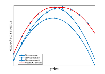
Figure 1: Revenue curves under three different parameters (blue), and the optimistic revenue (red)

Intuitively, if we knew that generalized distance $\delta$ would be large, then trying prices far away from $\hat{p}$ is beneficial for both exploration and exploitation. By contrast, if we knew that $\delta$ would be small, then striking a balance between exploration and exploitation would be very important, because choosing prices close to $\hat{p}$ is only effective for exploitation but not for exploration. Of course, the seller does not know the true value of $\delta$, which makes designing a learning algorithm that achieves the right balance between exploration and exploitation a more challenging task. O3FU algorithm achieves this objective by maximizing the optimistic revenue, which is defined as $\max_{\theta\in\mathcal{C}_{t-1}\cap\Theta^{{\dagger}}}p(\alpha+\beta p)$, and can be treated as the estimated revenue plus a “bonus” of exploration. In fact, as implied from equation (19.8) in Lattimore and Szepesvári (2018), when $\mathcal{C}_{t-1}\subseteq\Theta^{{\dagger}}$, we have $\max_{\theta\in\mathcal{C}_{t-1}\cap\Theta^{{\dagger}}}p(\alpha+\beta p)=p(\hat{\alpha}_{t-1}+\hat{\beta}_{t-1}p)+w_{t-1}\sqrt{[1\,\,p]V_{t-1,n}^{-1}[1\,\,p]^{\top}}$. Therefore, exploitation and exploration are both incorporated into the objective function through the first term and the second term, respectively.

It’s worth noting that our O3FU algorithm is parameter-free in the sense that it does not need to use any information about $\delta$. In addition, while O3FU algorithm takes $T$ as input, one can easily extend the current algorithm to work with unknown $T$ using the standard doubling trick (see, e.g., Lattimore and Szepesvári 2018) and construct an anytime algorithm that does not need to know $T$.

We now provide an upper bound on the regret of O3FU algorithm.

Theorem 3.1

Let $\pi$ be O3FU algorithm. Then there exists a finite constant $K_{1}>0$ such that for any $T\geq 1$, $n\geq 0$ and $\hat{p}\in[l,u]$, and for any possible value of $\theta^{*}\in\Theta^{{\dagger}}$,

$$R^{\pi}_{\theta^{*}}(T)\leq K_{1}\cdot\Big{(}\sqrt{T}\wedge\frac{T\log T}{(n\wedge T)\delta^{2}}\Big{)}\cdot\log T.$$

Theorem 3.1 provides a regret upper bound $\widetilde{\mathcal{O}}(\sqrt{T}\wedge\frac{T\log T}{(n\wedge T)\delta^{2}})$ that depends on the problem instance through the value of $\delta$, which is therefore called the instance-dependent upper bound. If $\delta$ is a constant, when $n=0$ or $n=\infty$, i.e., there are no offline data or infinitely many offline data under price $\hat{p}$, the upper bound reduces to $\widetilde{\mathcal{O}}(\sqrt{T})$ and $\widetilde{\mathcal{O}}(\log T)$ respectively. If $\delta$ is not a constant, with an order shrinking to zero as $T$ grows, the regret upper bound is then inversely proportional to $\delta^{2}$. We summarize the regret upper bound under different $(n,\delta)$ combinations in Table 3 of Appendix H.

We next outline the key ideas to prove Theorem 3.1 and leave the detailed analysis to Appendix A.1. From the statement of Theorem 3.1, it suffices to show an instance-independent upper bound $\widetilde{\mathcal{O}}(\sqrt{T})$ and an instance-dependent upper bound $\widetilde{\mathcal{O}}(\frac{T}{(n\wedge T)\delta^{2}})$. The instance-independent bound can be proved using similar arguments from stochastic linear bandits, e.g., Abbasi-Yadkori et al. (2011), by noting that the expected revenue is the inner product of the unknown parameter $[\alpha\,\,\beta]$ and the action vector $[p\,\,p^{2}]$. Showing the instance-dependent bound is the novel part in our proof, which relies on the following crucial lemma.

Lemma 3.2

Suppose $T\geq T_{0}$, $\delta\geq\frac{\sqrt{2(\alpha_{\max}^{2}+\beta_{\max}^{2})}w_{T}}{\beta_{\max}^{2}n^{1/4}}$, and $\theta^{*}\in\mathcal{C}_{t}$ for each $t\in[T]$, then two sequences of events $\{U_{t,1}\}_{t=1}^{T}$ and $\{U_{t,2}\}_{t=2}^{T}$ also hold, where

$$U_{t,1}=\Big{\{}|p_{t}-\hat{p}|\geq\min\Big{\{}1-\frac{\sqrt{2}}{2},\,\frac{C_{0}}{2}\Big{\}}\cdot\delta\Big{\}},$$

$$U_{t,2}=\Big{\{}||\tilde{\theta}_{t}-\theta^{*}||^{2}\leq C_{2}\cdot\frac{w_{t-1}^{2}}{(n\wedge(t-1))\delta^{2}}\Big{\}},$$

and $C_{0}=\frac{l|\beta_{\max}|}{u|\beta_{\min}|}$, $C_{1}=4(C_{0}+1)^{2}C_{0}^{-2}\big{(}1+(4u+1)^{2}\big{)}$, $C_{2}=\max\Big{\{}4(u-l)^{2},\,2C_{1},\,4((4u+1)^{2}+1)(\min\{\frac{C_{0}^{2}}{4},(1-\frac{\sqrt{2}}{2})^{2}\})^{-1}\Big{\}}$, $T_{0}=\min\Big{\{}t\in\mathbb{N}:w_{t}\geq\sqrt{C}_{1}\beta_{\max}^{2}(2(\alpha_{\max}^{2}+\beta_{\max}^{2}))^{-1/2}\Big{\}}$.

Lemma 3.2 is interpreted as follows. When the optimal price has a certain distance from historical price $\hat{p}$, i.e., $\delta\geq\frac{\sqrt{2(\alpha_{\max}^{2}+\beta_{\max}^{2})}w_{T}}{\beta_{\max}^{2}n^{1/4}}$, given that the demand parameter $\theta^{*}$ belongs to the confidence ellipsoid $\mathcal{C}_{t}$ in each period $t$, the algorithm’s pricing sequence $\{p_{t}\}_{t=1}^{T}$ is also uniformly bounded away from $\hat{p}$ proportional to the unknown quantity $\delta$ (as implied by events $\{U_{t,1}\}_{t=1}^{T}$), and will gradually approach the true optimal price in a rate of $\mathcal{O}(\frac{w_{t}^{2}}{(n\wedge t)\delta^{2}})$ (as implied by events $\{U_{t,2}\}_{t=2}^{T}$). This implies that the algorithm can “adaptively” explore to a suitable degree, to create an efficient “collaboration” between the online prices and the historical price, while concurrently approaching the unknown optimal price. This property is nontrivial and cannot be implied from the existing analysis of the OFU-type algorithms. To prove this lemma, we conduct a period-by-period trajectory analysis of the random pricing sequence generated by our algorithm. Specifically, we find that the occurrence of $U_{t,2}$ relies on the joint occurrence of $U_{1,1},\ldots,U_{t-1,1}$, while the occurrence of $U_{t,2}$ (combined with the specific structure of the optimistic revenue curve) in turn leads to the occurrence of $U_{t,1}$. We thus introduce novel induction-based arguments to prove Lemma 3.2, see details in Appendix A.2. The induction-based arguments also explain why we set the initial price in the algorithm to be a boundary point (or any price that has a constant distance from $\hat{p}$), since this enables $U_{1,1}$ to occur.

We remark that for the stochastic linear bandit problem with a polytope action set, Abbasi-Yadkori et al. (2011) prove an instance-dependent upper bound of $\mathcal{O}(\frac{\log T}{\Delta})$, where $\Delta$ is defined as the sub-optimality gap between the rewards of the best and second best extremal points of the action set. We emphasize that their result and analysis cannot be applied to prove our instance-dependent upper bound due to the following reasons. First, the instance-dependent upper bound in our problem is developed to capture the effect of the generalized distance $\delta$ on the regret bound, which does not exist in the stochastic linear bandit problem. Second, the instance-dependent upper bound in Abbasi-Yadkori et al. (2011) relies on two strong conditions: (i) their algorithm only selects actions among the extremal points of the action set, and (ii) every sub-optimal action taken by their algorithm is bounded away from the optimal action by a reward gap $\Delta$. Such conditions only hold under their setting and assumptions. Our problem, however, has a quadratic objective function, with the optimal price being an interior point of the interval $[l,u]$, which requires the algorithm’s actions to converge to the optimal action. As a result, the sub-optimality gap $\Delta$ becomes zero, and standard arguments based on $\Delta$ do not work.

3.2 Lower Bound on Regret

In this subsection, we establish a lower bound on the performance of any algorithm for the OPOD problem with a single historical price. We first introduce the following set of admissible policies denoted by $\Pi^{\circ}$, which includes all the policies whose regret is guaranteed to be $\widetilde{\mathcal{O}}(\sqrt{T})$ for any possible value of demand parameter $\theta^{*}$, i.e.,

$$\Pi^{\circ}=\Big{\{}\pi\in\Pi:\,\sup_{\theta^{*}\in\Theta^{{\dagger}}}R^{\pi}_{\theta^{*}}(T)\leq K_{0}\sqrt{T}(\log T)^{\lambda_{0}}\Big{\}},$$ (3)

where $K_{0}>0$ and $\lambda_{0}\geq 0$ are arbitrary constants. Intuitively, $\Pi^{\circ}$ excludes those “bad” policies that are not robust and suffer from large worst-case regret, e.g., a policy that never explores and always chooses $\hat{p}$, incurring zero regret when $\delta=0$ but linear regret when $\delta=\Theta(1)$. Restricting our attention to $\Pi^{\circ}$ (which O3FU and many existing algorithms obviously belong to) ensures that the considered policies are reasonable enough. Note that $\Pi^{\circ}$ is specified by a pair of $(K_{0},\lambda_{0})$, but for simplicity, when there is no ambiguity, we drop the dependence on $(K_{0},\lambda_{0})$ in the notation. To facilitate our discussion, let $R_{\theta}^{\pi}(T,n,\delta)$ be defined as the regret for admissible policy $\pi\in\Pi^{\circ}$ when the demand parameter is $\theta=(\alpha,\beta)$, i.e., $R^{\pi}_{\theta}(T,n,\delta)=T\cdot r^{*}(\theta)-\mathbb{E}^{\pi}_{\theta}[\sum_{t=1}^{T}r(p_{t};\theta)]$. We also denote $\mathcal{D}$ as the generic distribution of $\{\hat{\varepsilon}_{i}\}_{i=1}^{n}$ and $\{\varepsilon_{t}\}_{t=1}^{T}$, and $\mathcal{E}(R)$ as the class of sub-Gaussian distributions with parameter $R$.

The following theorem provides a regret lower bound for any admissible policy in terms of the generalized distance $\delta$. For any generalized distance $\delta$, we define an instance-dependent environment class $\{\theta\in\Theta^{{\dagger}}:|\hat{p}-\psi(\theta)|\in[(1-\xi)\delta,(1+\xi)\delta]\}$, which is the set of all possible values of the demand parameter whose associated optimal prices are $\Theta(\delta)$-distance away from $\hat{p}$ (here $\xi$ can be any fixed constant in $(0,1)$). This environment class highlights the role of $\delta$ as a key instance-dependent quantity, and enables us to establish an instance-dependent regret lower bound that holds for all possible values of $\delta$; see Theorem 3.3 (note that the environment class appears under the $\sup$ operator in the LHS of (6)).

Theorem 3.3

There exists a positive constant $K_{2}$ such that for any admissible policy $\pi\in\Pi^{\circ}$, for any $\xi\in(0,1)$, $T\geq 2$ and $n\geq 0$, and for any $\delta\in[0,u-l]$,

$$\sup_{\mathcal{D}\in\mathcal{E}(R);\atop\theta\in\Theta^{{\dagger}}:|\hat{p}-\psi(\theta)|\in[(1-\xi)\delta,(1+\xi)\delta]}R^{\pi}_{\theta}(T,n,\delta)\geq\left\{\begin{array}[]{ll}K_{2}\cdot\left((\sqrt{T}\wedge\frac{T}{(n\wedge T)\delta^{2}})\vee\log T\right),&\text{if }\delta\gtrsim T^{-\frac{1}{4}};\\ K_{2}\cdot\left((T\delta^{2})\vee\frac{\sqrt{T}}{(\log T)^{\lambda_{0}}}\right),&\text{if }\delta\lesssim T^{-\frac{1}{4}}.\end{array}\right.$$ (6)

Remark 3.4

We emphasize that finding a “right” definition of the instance-dependent environment class is important for capturing the true role of $\delta$ in determining the instance-dependent regret. While there may be other ways to specify the environment class, they may fail to accurately reflect the instance-dependent complexity of the OPOD problem. For example, if one sets the environment class to be the entire parameter space $\Theta^{\dagger}$, then one can obtain a single lower bound for the worst-case regret (independent of $\delta$); however, such a definition is too conservative and does not fully capture the value of offline data. Another seemingly natural way to specify the environment class is to consider $\{\theta\in\Theta^{{\dagger}}:|\psi(\theta)-\hat{p}|=\delta\}$, which is the set of all possible values of the demand parameter whose associated optimal price has a distance from $\hat{p}$ exactly equal to $\delta$. However, this definition cannot preclude certain speculative behavior of algorithms, and would result in an unrealistic regret bound that cannot be attained by any single algorithm. We refer to Appendix D for more details regarding the limitations of the above two definitions of the environment class.

We explain Theorem 3.3 as follows. First, when $\delta\gtrsim T^{-\frac{1}{4}}$, the regret lower bound is $\Omega((\sqrt{T}\wedge\frac{T}{(n\wedge T)\delta^{2}})\vee\log T)$, and in particular, if $\delta$ is a constant and $n=\infty$, the regret lower bound reduces to $\Omega(\log T)$, which recovers Theorem 3 in Keskin and Zeevi (2014) for their incumbent-price setting. Second, when $\delta\lesssim T^{-\frac{1}{4}}$, the regret lower bound is always $\widetilde{\Omega}(\sqrt{T})$, regardless of offline sample size $n$. The intuition is as follows. When restricting attention to $\Pi^{\circ}$, we exclude those “unreasonable” policies that seldom explore but make pricing decisions in a naive way, e.g., the one that always chooses price $\hat{p}+\delta$, because the regret of such policies cannot always be upper bounded by $\widetilde{\mathcal{O}}(\sqrt{T})$ for any possible value of $\theta^{*}$. In this case, any admissible policy $\pi\in\Pi^{\circ}$ should be able to make sufficient exploration to distinguish between different demand curves. However, to achieve this, the policy must deviate from $\hat{p}$, which is less informative since the seller already has collected some data under this price, to gain more information about the true demand curve. When $\delta$ is very small, charging prices away from $\hat{p}$ leads to a significant gap relative to the optimal price, and therefore a large regret bound. We summarize the regret lower bound under different $(n,\delta)$ combinations in Table 4 of Appendix H.

We next highlight the key steps in proving Theorem 3.3 and leave the detailed analysis to Appendix A.3. The proof idea is to reduce the OPOD problem to a hybrid of an estimation problem (see Step 1) and a hypothesis testing problem (see Step 2).

Step 1. In this step, we prove that when $\varepsilon$ follows a normal distribution, for any pricing policy $\pi\in\Pi$ (not necessarily in $\Pi^{\circ}$),

$$\sup_{\theta\in\Theta^{{\dagger}}:|\hat{p}-\psi(\theta)|\in[(1-\xi)\delta,(1+\xi)\delta]}R^{\pi}_{\theta}(T,n,\delta)=\Omega\Big{(}\big{(}\sqrt{T}\wedge\big{(}\frac{T}{\delta^{-2}+(n\wedge T)\delta^{2}}\big{)}\big{)}\vee\log(1+T\delta^{2})\Big{)}.$$ (7)

To prove (7), we consider an “auxiliary” estimation problem for the optimal price $\psi(\theta)$, and appeal to the multivariate van Trees inequality (cf. Gill and Levit 2001) to construct a lower bound for the Bayesian regret. In particular, when applying the van Trees inequality, we need to carefully choose a suitable instance-dependent prior distribution $q(\cdot)$ whose Fisher information grows at an appropriate rate with respect to $\delta$, and upper-bound the resulting Fisher information of the sequential estimators $\{p_{t}\}_{t=1}^{T}$ in different cases. Then we can rightly control the growth rate of the Bayesian regret.

Step 2. In the second step, we show that when $\varepsilon$ follows a normal distribution and $\delta\lesssim T^{-\frac{1}{4}}(\log T)^{-\frac{1}{2}\lambda_{0}}$, for any admissible policy $\pi\in\Pi^{\circ}$, there exists $\theta\in\Theta^{{\dagger}}$ satisfying $|\psi(\theta)-\hat{p}|\in[(1-\xi)\delta,(1+\xi)\delta]$ such that

$$R^{\pi}_{\theta}(T,n,\delta)=\Omega\Big{(}\frac{\sqrt{T}}{(\log T)^{\lambda_{0}}}\Big{)}.$$ (8)

The proof of (8) is based on arguments using Kullback-Leibler divergence and Bretagnolle-Huber inequality (Theorem 2.2 in Tsybakov 2009), whose key idea is as follows. We construct two problem instances with parameters $\theta_{1}$ and $\theta_{2}$ such that (i) the two demand curves under $\theta_{1}$ and $\theta_{2}$ intersect at price $\hat{p}$; (ii) the optimal prices under $\theta_{1}$ and $\theta_{2}$ are $\hat{p}+\delta$ and $\hat{p}+\delta+\Delta$ respectively, with $\Delta=\Theta(T^{-\frac{1}{4}}(\log T)^{\frac{1}{2}\lambda_{0}})$. For any pricing policy $\pi\in\Pi^{\circ}$, it has to perform well under both constructed problem instances, i.e., the regret upper bound is $\mathcal{\widetilde{O}}(\sqrt{T})$ under either instance, and therefore should be able to distinguish between the demand environments under $\theta_{1}$ and $\theta_{2}$. Moreover, any policy with the goal of separating $\theta_{1}$ and $\theta_{2}$ should charge prices significantly different from the intersected price $\hat{p}$, i.e., the KL-divergence between the two probability measures under $\theta_{1}$ and $\theta_{2}$ induced by policy $\pi$ is large. Nevertheless, since the optimal price associated with $\theta_{1}$ is $\hat{p}+\delta$, which is extremely close to $\hat{p}$, the policy will incur large regret when the underlying parameter is in fact $\theta_{1}$. Therefore, the regret under $\theta_{1}$ is always lower bounded by $\Omega(\frac{\sqrt{T}}{(\log T)^{\lambda_{0}}})$ no matter how large $n$ is.

3.3 Phase Transitions and Inverse-Square Law

In this subsection, we discuss two important implications. By comparing Theorems 3.1 and 3.3, one can easily verify that the regret upper bound $\widetilde{\mathcal{O}}(\sqrt{T}\wedge\frac{T\log T}{(n\wedge T)\delta^{2}})$ achieved by O3FU algorithm, after ignoring the logarithm factor, is unimprovable within the class of all admissible policies under the instance-dependent environment class considered in Theorem 3.3. Motivated by this result, for $\Pi^{\circ}$ with $\lambda_{0}\geq 1$, we define the optimal (instance-dependent) regret $R^{*}(T,n,\delta)$ as

$$R^{*}(T,n,\delta)=\inf_{\pi\in\Pi^{\circ}}\sup_{\mathcal{D}\in\mathcal{E}(R);\atop\theta\in\Theta^{{\dagger}}:|\psi(\theta)-\hat{p}|\in[(1-\xi)\delta,(1+\xi)\delta]}R^{\pi}_{\theta}(T).$$ (9)

Thus, $R^{*}(T,n,\delta)$ characterizes the statistical complexity of the OPOD problem in the sense that no algorithm in the admissible policy class can perform better than this rate when the true optimal price is allowed to center around $\hat{p}$ within $\Theta(\delta)$. We state this result in the following corollary.

Corollary 3.5

The optimal regret defined in (9) for the single-historical-price setting is

$$R^{*}(T,n,\delta)=\widetilde{\Theta}\left(\sqrt{T}\wedge\left(\frac{T}{n\delta^{2}}\vee\frac{\log T}{\delta^{2}}\right)\right).$$

The characterization of the optimal regret leads to two important implications. First, the decaying patterns of the optimal regret rate are different when offline sample size $n$ belongs to different ranges. To better illustrate this phenomenon, we first consider the well-separated case where $\delta$ is a constant independent of $T$. This case frequently happens in reality as it suggests that the seller’s historical price is suboptimal and quite different from the true optimal price. In this case, as $n$ increases, the optimal regret rate first remains at the level of $\widetilde{\Theta}(\sqrt{T})$ when $n\lesssim\sqrt{T}$, then gradually decays according to $\widetilde{\Theta}(\frac{T}{n})$ when $\sqrt{T}\lesssim n\lesssim T$, and finally reaches $\widetilde{\Theta}(\log T)$ when $n\gtrsim T$. This is depicted in Figure 2, from which we can clearly see that there are three ranges of $n$, i.e., $0<n\lesssim\sqrt{T}$, $\sqrt{T}\lesssim n\lesssim T$ and $n\gtrsim T$, referred to as the first, second and third phase respectively, and the optimal regret shows different properties in different phases. We refer to the significant transitions between the regret-decaying patterns of different phases as phase transitions.

Figure 2: Phase transitions for the single-historical-price setting with constant $\delta$

In contrast to the well-separated case where the phase transitions do not depend on the value of $\delta$, in the general case where $\delta$ may be very small, we cannot simply ignore the effect of $\delta$ in the optimal regret, and as a result, the number of phases and the thresholds of the offline sample size that define different phases are closely related to the magnitude of $\delta$. As illustrated in Figure 3, when $\delta=\widetilde{\Omega}(T^{-\frac{1}{4}})$, similar to the well-separated case, there are three phases defined by two thresholds of $n$: the optimal regret remains at the level of $\widetilde{\Theta}(\sqrt{T})$ in the first phase, and gradually decays according to $\widetilde{\Theta}(\frac{T}{n\delta^{2}})$ in the second phase, and stays at the level of $\widetilde{\Theta}(\frac{\log T}{\delta^{2}})$ in the third phase. When $\delta=\widetilde{\mathcal{O}}(T^{-\frac{1}{4}})$, there is no phase transition, and the optimal regret rate is always $\widetilde{\Theta}(\sqrt{T})$.

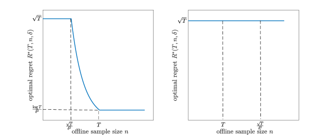
Figure 3: Phase transitions for the single-historical-price setting with general $\delta$. Left figure: $\delta\gtrsim T^{-\frac{1}{4}}$; right figure: $\delta\lesssim T^{-\frac{1}{4}}$

Second, Corollary 3.5 also characterizes the impact of the location of offline data relative to the optimal price on the optimal regret, which can be stated in the following inverse-square law: whenever offline data take effect, i.e., $\delta=\widetilde{\Omega}(T^{-\frac{1}{4}})$, and $n$ is in the second phase or the third phase, the optimal regret is inversely proportional to the square of generalized distance $\delta$. Therefore, the factor $\delta^{-2}$ is intrinsic in the regret bound. Seemingly counter-intuitive, the inverse-square law indicates that the closer the historical price is to the optimal price, the more difficult it is to learn the demand parameter, and the larger the optimal regret will be. In fact, this is a consequence of the exploration-exploitation trade-off. In the presence of offline data, a “good” learning algorithm needs to deviate from historical price $\hat{p}$ to conduct price experimentation. However, when $\delta$ is extremely small, such a deviation will also lead to a significant gap with the optimal price, and therefore incurs greater revenue loss to the seller. In an extreme case when the historical price happens to be the optimal price, i.e., $\delta=0$, even if $n=\infty$, the optimal regret is always $\widetilde{\Theta}(\sqrt{T})$.

4 Multiple Historical Prices

In this section, we consider the multiple-historical-price setting, where the $n$ historical prices can be different. In this case, $\sigma$ can be strictly positive and will play an important role to further reducing the complexity of the online learning task.

4.1 M-O3FU Algorithm and Regret Upper Bound

In this subsection, we develop a learning algorithm for the multiple-historical-price setting. We first make the following observations.

1. If $n\sigma^{2}\gtrsim\sqrt{T}$ and $\delta\lesssim T^{-\frac{1}{4}}$, then the offline data provide so much information that there is no need for online learning. In fact, by simply running linear regression on the offline data, we can obtain the estimate $\hat{\theta}_{0}$ for the true demand parameter with the squared estimation error of $\mathcal{O}(\frac{1}{n\sigma^{2}})$, i.e., $\mathbb{E}[||\hat{\theta}_{0}-\theta^{*}||^{2}]=\mathcal{O}(\frac{1}{n\sigma^{2}})$, which means that by simply charging price $\psi(\hat{\theta}_{0})$ in each online period, we achieve the regret of $\mathcal{O}(\frac{T}{n\sigma^{2}})$. Note that this $\mathcal{O}({\frac{1}{n\sigma^{2}}})$-type estimation error cannot be further improved in the online process by policies within $\Pi^{\circ}$, since when $T\delta^{2}\lesssim\sqrt{T}\lesssim n\sigma^{2}$, we have

   $$\mathbb{E}[J(\hat{p}_{1},\ldots,\hat{p}_{n},p_{1},\ldots,p_{T})] \leq 2\Big{(}\mathbb{E}[J(\hat{p}_{1},\ldots,\hat{p}_{n})]+\sum_{t=1}^{T}\mathbb{E}[(p_{t}-p^{*})^{2}]+T(\bar{p}_{1:n}-p^{*})^{2}\Big{)}\lesssim n\sigma^{2},$$ (10)

   where $J(x_{1},x_{2},\ldots,x_{k}):=\sum_{i=1}^{k}(x_{i}-\frac{1}{k}\sum_{j=1}^{k}x_{j})^{2}$ for any sequence $\{x_{i}\}_{i=1}^{k}$ and $k\geq 1$. This suggests that in the online process, exploration is “useless” in the sense that it cannot bring any theoretical improvement (in terms of reducing the order of estimation error) beyond offline regression. Therefore, if the algorithm knew that conditions $n\sigma^{2}\gtrsim\sqrt{T}$ and $\delta\lesssim T^{-\frac{1}{4}}$ hold, then there is no exploration-exploitation trade-off at all.

2. If in addition to the conditions in (i), a further extreme condition $\delta^{2}\lesssim\frac{1}{n\sigma^{2}}$ occurs, then even the above offline-regression-based approach may still be conservative: if an algorithm knew that $\delta^{2}\lesssim\frac{1}{n\sigma^{2}}\lesssim\frac{1}{\sqrt{T}}$, then by simply charging $\bar{p}_{1:n}$ in every online period, it achieves the regret of ${\mathcal{O}}(T\delta^{2})$, which is even better than ${\mathcal{O}}(\frac{T}{n\sigma^{2}})$. We refer to $\delta^{2}\lesssim\frac{1}{n\sigma^{2}}\lesssim\frac{1}{\sqrt{T}}$ as the corner case, and its complement as the regular case.

3. However, since the algorithm does not know the value of $\delta$ in advance, it does not know whether it is in the corner case (i.e., whether $\delta^{2}\lesssim\frac{1}{n\sigma^{2}}\lesssim\frac{1}{\sqrt{T}}$ is true) in advance. If the conditions in (i) do not hold, then the algorithm still needs online exploration; if the condition in (ii) does not hold, then the algorithm still needs offline regression.

Motivated by the above observations, we design the following Modified O3FU (M-O3FU) algorithm. With an abuse of terminology, we refer to O3FU algorithm in this section as the one proposed in §3.1 after natural modification to the multiple-historical-price setting by letting $V_{0,n}=\lambda I+\sum_{i=1}^{n}[1\,\,\hat{p}_{i}]^{\top}[1\,\,\hat{p}_{i}]$, $Y_{0,n}=\sum_{i=1}^{n}\hat{D}_{i}[1\,\,\hat{p}_{i}]^{\top}$, and $p_{1}=l\cdot\mathbb{I}\{\bar{p}_{1:n}>\frac{u+l}{2}\}+u\cdot\mathbb{I}\{\bar{p}_{1:n}\leq\frac{u+l}{2}\}$.

Input: offline data $\{(\hat{p}_{i},\hat{D}_{i})\}_{i=1}^{n}$, support of demand parameters $\Theta^{{\dagger}}$, price range $[l,u]$, regularization parameter $\lambda=1+u^{2}$, $\{w_{t}\}_{t\geq 0}$ defined in (2) with $\epsilon=\frac{1}{T^{2}}\wedge\frac{1}{n\sigma^{2}}$, parameter $K>1$;

Initialization: $V_{0,n}=\lambda I+\sum_{i=1}^{n}[1\,\,\hat{p}_{i}]^{\mathsf{T}}[1\,\,\hat{p}_{i}]$, $Y_{0,n}=\sum_{i=1}^{n}\hat{D}_{i}[1\,\,\hat{p}_{i}]^{\mathsf{T}}$, $\hat{\theta}_{0}=V_{0,n}^{-1}Y_{0,n}$, $\mathcal{C}_{0}=\{\theta\in\Theta^{{\dagger}}:||\theta-\hat{\theta}_{0}||_{V_{0,n}}\leq w_{0}\}$;

if $\frac{\min_{\theta\in\mathcal{C}_{0}}|\bar{p}_{1:n}-\psi(\theta)|}{\max_{\theta_{1},\theta_{2}\in\mathcal{C}_{0}}|\psi(\theta_{1})-\psi(\theta_{2})|}\leq K$, and $n\sigma^{2}\geq\sqrt{T}$ then

      Charge price $p_{t}=\bar{p}_{1:n}$ for each $t\in[T]$;

else

      Run O3FU Algorithm.

Algorithm 2 M-O3FU Algorithm

We next make several highlights about M-O3FU algorithm. First, in comparison with O3FU algorithm, before the start of the online learning process, M-O3FU algorithm takes a preliminary step that tests whether the distance between $\bar{p}_{1:n}$ and interval $\{\psi(\theta):\theta\in\mathcal{C}_{0}\}$ is smaller than a constant times the length of interval $\{\psi(\theta):\theta\in\mathcal{C}_{0}\}$. The goal of this step is to test whether condition $\delta^{2}\lesssim\frac{1}{n\sigma^{2}}$ holds or not. If this condition is inferred to hold based on the empirical observation, and in addition, $n\sigma^{2}\geq\sqrt{T}$, the algorithm keeps using $\bar{p}_{1:n}$ for each online period. Otherwise, the algorithm simply runs O3FU algorithm. Second, parameter $\epsilon$ defined in $w_{t}$ is modified from $\frac{1}{T^{2}}$ (used in O3FU) to $\frac{1}{T^{2}}\wedge\frac{1}{n\sigma^{2}}$, which guarantees that $\theta^{*}$ belongs to each confidence ellipsoid $\mathcal{C}_{t}$ with sufficiently high probability, and the revenue loss incurred when $\theta^{*}$ does not belong to some confidence ellipsoid can be bounded by $\mathcal{O}(\frac{T}{n\sigma^{2}}\wedge\frac{1}{T})$.

The following theorem provides an upper bound on the regret of M-O3FU algorithm.

Theorem 4.1

Let $\pi$ be M-O3FU algorithm. Then there exists a finite constant $K_{3}>0$ such that for any $T\geq 1$, $n\geq 0$, $\sigma\geq 0$ and $\bar{p}_{1:n}\in[l,u]$, and for any possible value of $\theta^{*}\in\Theta^{{\dagger}}$, we have

$$R^{\pi}_{\theta^{*}}(T)\leq\left\{\begin{array}[]{ll}K_{3}\cdot\big{(}T\delta^{2}+1\big{)},&\text{if }\delta^{2}\lesssim\frac{1}{n\sigma^{2}}\lesssim\frac{1}{\sqrt{T}};\\ K_{3}\cdot\Big{(}\big{(}\sqrt{T}\log T\big{)}\wedge\frac{T(\log T)^{2}}{n\sigma^{2}+(n\wedge T)\delta^{2}}+1\Big{)},&\text{otherwise}.\\ \end{array}\right.$$

Theorem 4.1 shows that the regret upper bound has different forms in two different cases. When $\delta^{2}\lesssim\frac{1}{n\sigma^{2}}\lesssim\frac{1}{\sqrt{T}}$, M-O3FU algorithm achieves the regret upper bound $\mathcal{O}(T\delta^{2}+1)$, which matches the ideal regret bound in the above item (ii) discussed at the beginning of this subsection. Otherwise, the regret upper bound becomes $\widetilde{\mathcal{O}}(\sqrt{T}\wedge\frac{T}{n\sigma^{2}+(n\wedge T)\delta^{2}}+1)$. Compared with the upper bound in Theorem 3.1, there is an additional term $n\sigma^{2}$ in the denominator capturing the effect of the dispersion of offline data. We summarize the regret upper bound under different $(n,\sigma,\delta)$ combinations in Table 5 of Appendix H.

The proof of Theorem 4.1 can be found in Appendix B.1. Similar to the proof of Theorem 3.1, we also need an important technical lemma stated as follows.

Lemma 4.2

Suppose we run O3FU algorithm from $t=1$ with given input offline data $\{(\hat{p}_{i},\hat{D}_{i})\}_{i=1}^{n}$, $\sigma\leq\delta$, $\delta\geq\max\{\frac{\sqrt{2(\alpha_{\max}^{2}+\beta_{\max}^{2})}}{\beta_{\max}^{2}}\frac{T^{1/4}w_{T}}{n^{1/2}},\sqrt{C}_{1}T^{-1/4}\}$, and $\theta^{*}\in\mathcal{C}_{t}$ for each $t\in[T]$, then two sequences of events $\{U_{t,3}\}_{t=1}^{T}$ and $\{U_{t,4}\}_{t=2}^{T}$ also hold, where

$$U_{t,3}=\Big{\{}|p_{t}-\bar{p}_{1:n}|\geq\min\big{\{}1-\frac{\sqrt{2}}{2},\frac{C_{0}}{2}\big{\}}\cdot\delta\Big{\}},$$

$$U_{t,4}=\Big{\{}||\tilde{\theta}_{t}-\theta^{*}||^{2}\leq C_{3}\frac{w_{t-1}^{2}}{n\sigma^{2}+(n\wedge(t-1))\delta^{2}}\Big{\}},$$

and $C_{0}$ and $C_{1}$ are defined in Lemma 3.2, and $C_{3}=\max\Big{\{}8(u-l)^{2},4C_{1},2\max\{2(\sqrt{2}+1)^{2},\frac{4}{C_{0}^{2}}\}\cdot((4u+1)^{2}+1)\Big{\}}.$

Similar to Lemma 3.2, Lemma 4.2 is also proved based on induction arguments. Besides, we need to use the following lower bound on the sum of squared price deviations:

$$J(\hat{p}_{1},\ldots,\hat{p}_{n},p_{1},\ldots,p_{t}) \geq J(\hat{p}_{1},\ldots,\hat{p}_{n})+\frac{n}{n+t}\sum_{s=1}^{t}(p_{s}-\bar{p}_{1:n})^{2},$$ (11)

where $J(x_{1},x_{2},\ldots,x_{k}):=\sum_{i=1}^{k}(x_{i}-\frac{1}{k}\sum_{j=1}^{k}x_{j})^{2}$ for any sequence $\{x_{i}\}_{i=1}^{k}$ and $k\geq 1$. We can interpret $J(x_{1},x_{2},\ldots,x_{k})$ as the information metric capturing the variation for a sequence $\{x_{i}\}_{i=1}^{k}$. Then inequality (11) bounds the information accumulated up to period $t$ from below, through the pre-existing offline information, plus the information due to the deviation of the algorithm’s prices from the average historical price. The proof of Lemma 4.2 is provided in Appendix B.2.

4.2 Lower Bound on Regret

In this subsection, we establish a lower bound on the best-achievable regret for the OPOD problem among the class of admissible policies $\Pi^{\circ}$ defined in a similar way to (3). Again, we denote $R_{\theta}^{\pi}(T,n,\delta,\sigma)$ as the regret incurred by policy $\pi\in\Pi^{\circ}$ under the demand parameter $\theta$.

Theorem 4.3

There exists a positive constant $K_{4}$ such that for any admissible policy $\pi\in\Pi^{\circ}$, for any $\xi\in(0,1)$, $T\geq 2$, $n\geq 0$ and $\sigma\geq 0$, and for any $\delta\in[0,u-l]$,

$$\sup_{\mathcal{D}\in\mathcal{E}(R);\atop\theta\in\Theta^{{\dagger}}:|\bar{p}_{1:n}-\psi(\theta)|\in[(1-\xi)\delta,(1+\xi)\delta]}R^{\pi}_{\theta}(T,n,\delta,\sigma)\geq\left\{\begin{array}[]{ll}K_{4}\cdot T\delta^{2},&\text{if }\delta^{2}\lesssim\frac{1}{n\sigma^{2}}\lesssim\frac{1}{\sqrt{T}};\\ K_{4}\cdot\Big{(}\frac{\sqrt{T}}{(\log T)^{\lambda_{0}}}\wedge\frac{T}{n\sigma^{2}+(n\wedge T)\delta^{2}}\Big{)},&\text{otherwise}.\end{array}\right.$$

Similar to Theorem 3.3, the instance-dependent environment class is defined as the set of instances whose associated optimal prices are away from $\bar{p}_{1:n}$ by a distance $\Theta(\delta)$. Since M-O3FU algorithm achieves the regret upper bound $\mathcal{O}(\sqrt{T}\log T)$ for any value of $\theta^{*}\in\Theta^{{\dagger}}$ (thus belongs to the admissible policy class $\Pi^{\circ}$ with $\lambda_{0}\geq 1$), Theorem 4.3 demonstrates that for both the corner and regular cases, the regret rate achieved by M-O3FU algorithm in Theorem 4.1 cannot be further improved by any policy in $\Pi^{\circ}$. The proof of Theorem 4.3 is provided in Appendix B.4, which is a generalization to that of Theorem 3.3. We also summarize the regret lower bound under different $(n,\sigma,\delta)$ combinations in Table 6 of Appendix H.

4.3 Phase Transitions and Generalized Inverse-Square Law

Motivated from the matching upper and lower bounds (after ignoring logarithm factors) in Theorems 4.1 and 4.3 respectively, we define the optimal instance-dependent regret for the OPOD problem in the multiple-historical-price setting as follows:

$$R^{*}(T,n,\delta,\sigma)=\inf_{\pi\in\Pi^{\circ}}\sup_{\mathcal{D}\in\mathcal{E}(R);\atop\theta\in\Theta^{{\dagger}}:|\psi(\theta)-\bar{p}_{1:n}|\in[(1-\xi)\delta,(1+\xi)\delta]}R^{\pi}_{\theta}(T,n,\delta,\sigma),$$ (12)

where a slight difference compared with (9) is the modification from the single historical price $\hat{p}$ to the average historical price $\bar{p}_{1:n}$.

Combining Theorem 4.1 and Theorem 4.3, we are able to characterize the optimal regret of the OPOD problem for the multiple-historical-price setting.

Corollary 4.4

The optimal regret defined in (12) for the multiple-historical-price setting is

$$R^{*}(T,n,\delta,\sigma)=\left\{\begin{array}[]{ll}\widetilde{\Theta}\Big{(}\sqrt{T}\wedge\frac{T}{n\sigma^{2}+(n\wedge T)\delta^{2}}\Big{)},&\text{for the regular case};\\ \widetilde{\Theta}\big{(}T\delta^{2}\big{)},&\text{for the corner case}.\end{array}\right.$$

Recall that in the single-historical-price setting, the threshold $\widetilde{\Theta}(T^{-\frac{1}{4}})$ of $\delta$ plays an important role in characterizing the behavior of the optimal regret rate. This threshold $\widetilde{\Theta}(T^{-\frac{1}{4}})$ also plays a role in the optimal regret rate of the multiple-historical-price setting.

When $\delta\gtrsim T^{-\frac{1}{4}}$, there are significant differences for the behaviors of the optimal regret rate, depending on whether $\sigma$ is less than, equal to or greater than $\delta$. This is illustrated in Figure 4, where the green, red and blue curves depict the above three cases respectively. If $\sigma=o(\delta)$, as shown in the green curve, the optimal regret rate exhibits four decaying patterns as $n$ changes between different ranges. Specifically, the optimal regret rate first remains at $\widetilde{\Theta}(\sqrt{T})$ when $n\lesssim\frac{\sqrt{T}}{\delta^{2}}$, and then decreases according to $\widetilde{\Theta}(\frac{T}{n\delta^{2}})$ when $\frac{\sqrt{T}}{\delta^{2}}\lesssim n\lesssim T$. After that, the optimal regret rate stays at $\widetilde{\Theta}(\frac{\log T}{\delta^{2}})$ when $T\lesssim n\lesssim\frac{T\delta^{2}}{\sigma^{2}}$, and finally, it decreases according to $\widetilde{\Theta}(\frac{T}{n\sigma^{2}})$ when $n\gtrsim\frac{T\delta^{2}}{\sigma^{2}}$. If $\sigma=\Theta(\delta)$ or $\sigma=\Omega(\delta)$ as shown in the red or blue curve, the optimal regret rate exhibits two phases: it remains at the level of $\widetilde{\Theta}(\sqrt{T})$ when $n\lesssim\frac{\sqrt{T}}{\sigma^{2}}$, and decays according to $\widetilde{\Theta}(\frac{T}{n\sigma^{2}})$ when $n\gtrsim\frac{\sqrt{T}}{\sigma^{2}}$. Therefore, when $\sigma$ gradually increases, depending on its magnitude compared with $\delta$, the number of phases of the optimal regret rate also experiences the change from four phases to two phases, and the entire patterns of the phase transitions of the optimal regret rate also change accordingly.

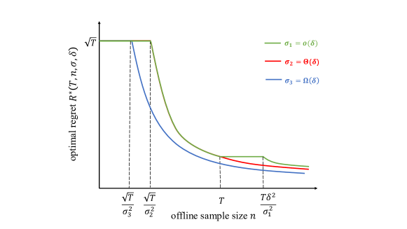
Figure 4: Multiple-historical-price setting with $\delta\gtrsim T^{-\frac{1}{4}}$ and different $\sigma$

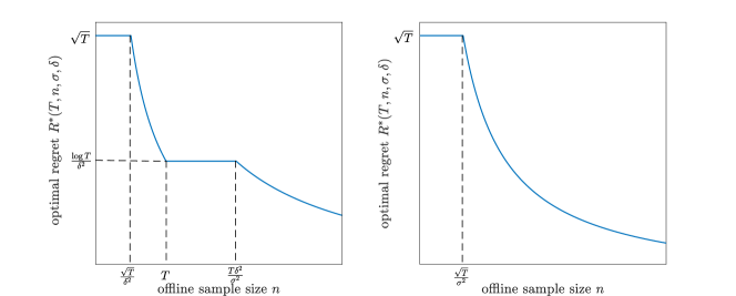
Figure 5: Phase transitions for the multiple-historical-price setting with $\delta\gtrsim T^{-\frac{1}{4}}$. Left figure: $\sigma=o(\delta)$; right figure: $\sigma=\Omega(\delta)$

Corollary 4.4 also reveals a generalized inverse-square law. Specifically, the optimal regret is inversely proportional to the square of both $\delta$ and $\sigma$, which quantifies the effect of the location and dispersion of the offline data on the optimal regret. The intuition for the dependence of the optimal regret on $\delta$ is similar to the single-historical-price setting. For the dependence of the optimal regret on $\sigma$, as the historical prices become more dispersive, i.e., $\sigma$ increases, the seller can obtain a more accurate estimate for the unknown demand parameter from offline regression, which helps to further reduce the optimal regret of the online learning process.

It’s also worth noting that the thresholds of the offline sample size that define different phases of the optimal regret depend on both $\delta$ and $\sigma$. When $\sigma=\mathcal{O}(\delta)$ and $\delta=\widetilde{\Omega}(T^{-\frac{1}{4}})$, the first threshold of $n$ that defines the first and second phases, i.e., $\widetilde{\Theta}(\frac{\sqrt{T}}{\delta^{2}})$, decreases in $\delta$. When $\sigma=\Omega(\delta)$ and $\delta=\widetilde{\Omega}(T^{-\frac{1}{4}})$, the threshold of $n$ that defines the first and second phases, i.e., $\widetilde{\Theta}(\frac{\sqrt{T}}{\sigma^{2}})$, decreases in the standard deviation $\sigma$. This implies that more offline data will be required to overcome the challenges caused by a shorter generalized distance $\delta$ or a smaller standard deviation $\sigma$.

When $\delta\lesssim T^{-\frac{1}{4}}$, Corollary 4.4 indicates that there are three phases of the optimal regret rate as $n$ changes. When $n\lesssim\frac{\sqrt{T}}{\delta^{2}}$, the optimal regret remains at $\widetilde{\Theta}(\sqrt{T})$. When $\frac{\sqrt{T}}{\delta^{2}}\lesssim n\lesssim\frac{1}{\delta^{2}\sigma^{2}}$, the optimal regret experiences a sudden drop from $\widetilde{\Theta}(\sqrt{T})$ to $\widetilde{\Theta}(T\delta^{2})$. When $n\gtrsim\frac{1}{\delta^{2}\sigma^{2}}$, the optimal regret decays according to $\widetilde{\Theta}(\frac{T}{n\sigma^{2}})$. Such transitions of the optimal regret with different $n$ are illustrated in Figure 6. In particular, the second phase corresponds to the corner case defined in §4.1. In this case, smaller $\delta$ leads to lower optimal regret, which is in contrast to the inverse-square law in the regular case. This is because in the corner case, as discussed in §4.1, there is no need for online learning and therefore no exploration-exploitation trade-off, and the policy that always charges $\bar{p}_{1:n}$ incurs very small regret. In this case, the closer the average historical price is to the optimal price, the smaller the optimal regret will be. By contrast, the inverse-square law in the regular case is a consequence of the exploration-exploitation trade-off.

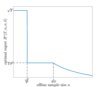
Figure 6: Phase transitions for the multiple-historical-price setting with $\delta\lesssim T^{-\frac{1}{4}}$

5 Numerical Study

In this section, we test the performance of our algorithm on a synthetic data set. We define the relative regret for a given learning algorithm $\pi$ as $\frac{Tp^{*}\cdot(\alpha^{*}+\beta^{*}p^{*})-\sum_{t=1}^{T}\mathbb{E}_{\theta^{*}}^{\pi}[p_{t}(\alpha^{*}+\beta^{*}p_{t})]}{Tp^{*}\cdot(\alpha^{*}+\beta^{*}p^{*})}\times 100\%$, and the following three problem instances are tested:

• $\theta^{*}=[2.6,-1.8]$, $[\alpha_{\min},\alpha_{\max}]=[2.5,3.5]$, $[\beta_{\min},\beta_{\max}]=[-2,-1.3]$, $[l,u]=[0.1,2]$, $R=2.2$;

• $\theta^{*}=[3.7,-3.15]$, $[\alpha_{\min},\alpha_{\max}]=[3.5,5]$, $[\beta_{\min},\beta_{\max}]=[-3.2,-2.5]$, $[l,u]=[0.5,1.3]$, $R=2.5$;

• $\theta^{*}=[2.9,-2.6]$, $[\alpha_{\min},\alpha_{\max}]=[2.8,3.5]$, $[\beta_{\min},\beta_{\max}]=[-2.8,-1]$, $[l,u]=[0.2,2]$, $R=1.8$.

and $\varepsilon$ follows a normal distribution with standard deviation $R$. For each of the above instance, we repeat the experiments for 500 times, and the results are computed after averaging over the 500 experiments. Under the multiple-historical-price setting, we test a simplified version of M-O3FU algorithm by directly running O3FU, without checking the preliminary condition. Thus, throughout this section, we simply call our algorithm “O3FU algorithm.”

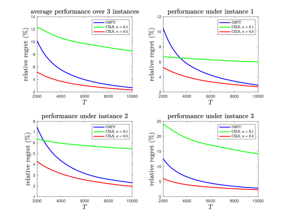
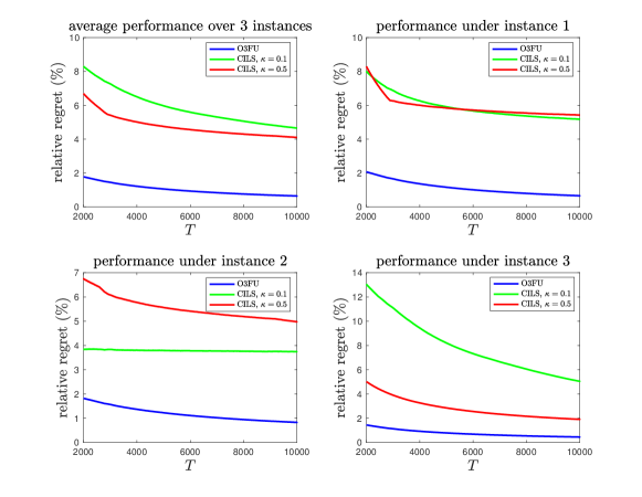
Figure 7: Comparison between O3FU and CILS when there are no offline data

Figure 8: Comparison between O3FU and CILS when there are $n=1000$ offline demand data

First, we compare our O3FU algorithm with the modified Constrained Iterated Least Squares (CILS) algorithm. When there are no offline data, we adopt CILS algorithm directly from Keskin and Zeevi (2014). When there are offline data, no existing learning algorithm in prior literature is directly suitable for this setting, so we make a natural modification to the original CILS by incorporating offline data into the least-square estimation. In both cases, we set the tuning parameter $\kappa$ in CILS to be $0.1$ following Keskin and Zeevi (2014), and also $0.5$ which seems to lead to the best performance of CILS. Figures 8 and 8 show the performances of O3FU and CILS algorithms for the settings when there are no offline data, and when there are $n=1000$ offline demand data under a single historical price (specifically, we set $\hat{p}=1.8,0.9,1$ for instances (1)-(3) respectively). As seen from Figure 8, without offline data, O3FU performs better than CILS with $\kappa=0.1$ and comparably to CILS with $\kappa=0.5$ as $T$ becomes larger. Figure 8 reveals that with the help of offline data, the regret of O3FU algorithm is significantly reduced for all $T$ under all instances. By contrast, for CILS algorithms, the impact of offline data on the empirical regret is not obvious and heavily relies on the tuning parameter and specific problem instance. For CILS with $\kappa=0.1$, the improvement of the relative regret is clear under instance (3), but rather minimal under instances (1) and (2). For CILS with $\kappa=0.5$, the regret only decreases a little under instance (3), and even becomes larger under instances (1) and (2). Therefore, compared with CILS algorithms, O3FU algorithm better exploits the value of offline data and is more robust to different problem instances.

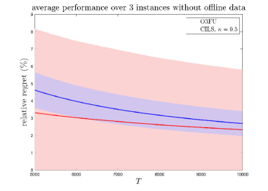
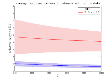
Figure 9: 95% confidence-region comparison between O3FU and CILS with $\kappa=0.5$

Second, Figure 9 plots the 95% confidence region of O3FU algorithm and CILS algorithm with $\kappa=0.5$, for both cases when there are no offline data and when there are $n=1000$ offline data. The left figure shows that while CILS with properly tuned parameter performs slightly better than O3FU on average when there are no offline data, the standard deviation of CILS among the 500 simulations is much larger than O3FU. This implies that O3FU is more stable than CILS. The right figure shows that with offline data, O3FU always outperforms CILS, in terms of both the average regret and standard deviation. Since O3FU algorithm has highly stable performance, we believe that it should be preferable in many real-life business settings.

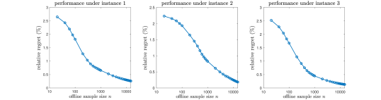
Figure 10: $T=10^{4}$-period relative regret for the single-historical-price setting with different $n$

Figure 11: $T=10^{4}$-period relative regret for the single-historical-price setting with different $\delta$

Figure 12: $T=10^{4}$-period relative regret for the multiple-historical-price setting with different $\sigma$

Third, we investigate the effect of offline sample size $n$ on the empirical regret of O3FU algorithm. In Figure 12, we plot the relative regret of O3FU algorithm given different amount of offline data (with $n$ ranging from 20 to 12000), under the single-historical-price setting (with $\hat{p}=1.8,0.9,1$ for instances (1)-(3) respectively). The x-axis is depicted on a log scale. We can see clearly that for each problem instance, as the offline sample size increases, the relative regret decreases, which is consistent with the phase transitions implied from our theoretical results.

Finally, we investigate the effects of generalized distance $\delta$ and price dispersion $\sigma$ on the empirical regret of our algorithm. Figure 12 shows the relative regret of O3FU algorithm given $n=500$ offline demand observations under historical price $p^{*}+\delta$ with different $\delta$, and Figure 12 shows the relative regret of O3FU algorithm given 250 offline demand observations under historical price $\bar{p}_{1:n}-\sigma$, and 250 offline demand observations under historical price $\bar{p}_{1:n}+\sigma$ with different $\sigma$, where $\bar{p}_{1:n}=0.8,0.8,0.7$ for instances (1)-(3) respectively. As seen from Figure 12 and 12, when $\delta$ or $\sigma$ increases, the empirical regret of our algorithm decays, which also matches the inverse-square law.

Remark 5.1

We remark that the empirical evidence for the phase transitions and inverse-square law is not always observed under every problem instance. This is because according to its definition through the supremum over some instance-dependent environment class, the optimal regret should be attained at some “hard” instances, and so do its implications of the phase transitions and inverse-square law. Besides, when discussing the optimal regret rate and its implications, we require $T$ to be sufficiently large, and ignore all the constant factors. Our choices of instances (1)-(3) capture the aforementioned hard instances, and also avoid that the problem falls into the regimes where constant factors significantly affect the overall regret rate.

6 Further Discussion: Offline Data and Self-Exploration

In M-O3FU algorithm proposed in §4.1, there is a preliminary step testing whether $\frac{\min_{\theta\in\mathcal{C}_{0}}|\bar{p}_{1:n}-\psi(\theta)|}{\max_{\theta_{1},\theta_{2}\in\mathcal{C}_{0}}|\psi(\theta_{1})-\psi(\theta_{2})|}\leq K$ holds or not. We find that this step also has an important implication in practice: $\frac{\min_{\theta\in\mathcal{C}_{0}}|\bar{p}_{1:n}-\psi(\theta)|}{\max_{\theta_{1},\theta_{2}\in\mathcal{C}_{0}}|\psi(\theta_{1})-\psi(\theta_{2})|}>K$ is actually a sufficient condition for self-exploration in our OPOD problem. That is, with high probability, when this condition holds, the myopic (i.e., greedy) policy can achieve the optimal regret without any active exploration.

The myopic policy is defined as follows. Let $\mathcal{C}_{0}=\{\theta\in\Theta^{{\dagger}}:||\theta-\theta_{0}^{\text{LS}}||^{2}_{V_{0,n}}\leq w_{0}^{2}\}$, where $V_{0,n}=\lambda I+\sum_{i=1}^{n}[1\,\,\hat{p}_{i}]^{\top}[1\,\,\hat{p}_{i}]$, $\theta_{0}^{\text{LS}}=\arg\min_{\theta\in\Theta^{{\dagger}}}\sum_{i=1}^{n}((\hat{D}_{i}-\alpha-\beta\hat{p}_{i})^{2}+\lambda(\alpha^{2}+\beta^{2}))$, and $w_{0}=R\sqrt{2\log((T^{2}\vee n\sigma^{2})(1+(1+u^{2})n/\lambda))}+\sqrt{\lambda(\alpha_{\max}^{2}+\beta_{\min}^{2})}$. Let $\{p_{t}^{\text{myopic}}\}_{t\geq 1}$ be the sequence of prices charged by the myopic policy. For $t=1$, $p_{t}^{\text{myopic}}=\psi(\theta_{0}^{\text{LS}})$, and for each $t\geq 2$, we first compute the least-square estimator $\theta_{t-1}^{\text{LS}}$ based on offline data and all the available online data within confidence ellipsoid $\mathcal{C}_{0}$:

$$\theta_{t-1}^{\text{LS}}=\arg\min_{\theta\in\mathcal{C}_{0}}\Big{(}\sum_{i=1}^{n}(\hat{D}_{i}-\alpha-\beta\hat{p}_{i})^{2}+\sum_{s=1}^{t-1}(D_{s}-\alpha-\beta p_{s})^{2}+\lambda(\alpha^{2}+\beta^{2})\Big{)},$$

and then let $p_{t}^{\text{myopic}}=\psi(\theta_{t-1}^{\text{LS}})$. The next proposition shows that the myopic policy is guaranteed to be optimal if certain condition holds.

Proposition 6.1

Suppose $n\sigma^{2}\geq\sqrt{T}$. Then with probability at least $1-\frac{1}{T^{2}}\wedge\frac{1}{n\sigma^{2}}$, the following event holds: if $\frac{\min_{\theta\in\mathcal{C}_{0}}|\bar{p}_{1:n}-\psi(\theta)|}{\max_{\theta_{1},\theta_{2}\in\mathcal{C}_{0}}|\psi(\theta_{1})-\psi(\theta_{2})|}>K$ for some $K>1$, then the myopic policy ensures that the regret is $\widetilde{\mathcal{O}}(\frac{T}{n\sigma^{2}+(n\wedge T)\delta^{2}})$.

The intuition of Proposition 6.1 is as follows. Note that the key step to prove the instance-dependent upper bound $\widetilde{\mathcal{O}}(\frac{T}{n\sigma^{2}+(n\wedge T)\delta^{2}})$ in Theorem 4.1 is to show events $\{U_{t,3}\}_{t=1}^{T}$ and $\{U_{t,4}\}_{t=2}^{T}$ in Lemma 4.2 hold. Since the myopic policy charges prices based on estimator $\theta_{t-1}^{\text{LS}}\in\mathcal{C}_{0}$ in each period $t$, and $\mathcal{C}_{0}$ contains $\theta$ with high probability, under the condition in Proposition 6.1, we can easily verify that the myopic price $p_{t}^{\text{myopic}}$ is bounded away from $\bar{p}_{1:n}$ by a distance proportional to $\delta$. In other words, event $U_{t,3}$ in Lemma 4.2 is automatically satisfied for each period $t$, and in this case, when $\theta^{*}\in\mathcal{C}_{t}=\{\theta\in\Theta^{{\dagger}}:||\theta-\theta_{t}^{\text{LS}}||^{2}_{V_{t,n}}\leq w_{t}^{2}\}$, we can further show that event $U_{t,4}$ also holds. Therefore, the myopic policy ensures that the regret is $\widetilde{\mathcal{O}}(\frac{T}{n\sigma^{2}+(n\wedge T)\delta^{2}})$.

We also make several remarks about Proposition 6.1. First, the interpretation of probability “$1-\frac{1}{T^{2}}\wedge\frac{1}{n\sigma^{2}}$” is similar to the interpretation of “95%” in a 95% confidence interval. Such a probabilistic statement is common in frequentist statistics, when one wants to make some inference (e.g., myopic policy is optimal or not) based on some empirical observations (e.g., $\frac{\min_{\theta\in\mathcal{C}_{0}}|\psi(\theta)-\bar{p}_{1:n}|}{\max_{\theta_{1},\theta_{2}\in\mathcal{C}_{0}}|\psi(\theta_{1})-\psi(\theta_{2})|}>K$). Second, if the regular case happens, i.e., $n\sigma^{2}\gtrsim\sqrt{T}$ and $\delta^{2}\gtrsim\frac{1}{n\sigma^{2}}$, one can easily verify that the empirical condition described in Proposition 6.1 always holds. In this case, the myopic algorithm always ensures $\widetilde{\mathcal{O}}(\frac{T}{n\sigma^{2}+(n\wedge T)\delta^{2}})$ regret. Nevertheless, verifying the condition $\delta^{2}\gtrsim\frac{1}{n\sigma^{2}}$ requires knowing the true parameter $\theta^{*}$ in advance, which is not practical in reality. Thus, we make a probabilistic statement in Proposition 6.1 about the regret bound under an empirical condition that can be directly verified by the algorithm. Third, the choice of $1-\frac{1}{T^{2}}\wedge\frac{1}{n\sigma^{2}}$ is not essential in Proposition 6.1. In fact, one can achieve any higher probability bound that is arbitrarily close to 1 by defining a larger confidence ellipsoid $\mathcal{C}_{0}$, although in that case, the condition $\frac{\min_{\theta\in\mathcal{C}_{0}}|\psi(\theta)-\bar{p}_{1:n}|}{\max_{\theta_{1},\theta_{2}\in\mathcal{C}_{0}}|\psi(\theta_{1})-\psi(\theta_{2})|}>K$ will be more difficult to be satisfied.

In reality, myopic policies are commonly adopted in many industries, since they are quite easy to explain to managers, and relatively simple to implement in practice. See the discussion of myopic policies in, e.g. Harrison et al. (2012), Keskin and Zeevi (2014), Qiang and Bayati (2016). However, due to the lack of active exploration, myopic policies typically suffer from incomplete learning, thus usually have poor theoretical performance in dynamic pricing. Proposition 6.1 shows how offline data may help myopic policies to achieve self-exploration in dynamic pricing: when there are enough dispersive offline data, then with high probability, as long as $\bar{p}_{1:n}$ is bounded away from offline confidence interval of $p^{*}$, the issue of incomplete learning could be resolved, and the myopic policy could achieve self-exploration.

7 Conclusion

In this paper, we investigate the impact of offline data on online learning in the context of dynamic pricing. In contrast to previous literature that involves only offline data or only online data, we consider a more practical problem involving both offline data and online data, aiming to understand whether and how the pre-existence of offline data would benefit the online learning process. For both single-historical-price and multiple-historical-price settings, we design a learning algorithm based on the OFU principle with a provable instance-dependent regret upper bound, and establish a regret lower bound that matches the upper bound up to logarithmic factors. Two important and nontrivial implications implied by our results are phase transitions and the inverse-square law, characterizing the joint effect of the size, location, and dispersion of the offline data on the optimal regret. The numerical experiments demonstrate the effectiveness, robustness and stability of our algorithm, and reveal the empirical evidence for phase transitions and the inverse-square law. Besides, we also develop a sufficient condition for the myopic policy to achieve the optimal regret in the regular case.

We discuss two extensions of this paper. First, while we focus on the linear demand model in this paper, the regret upper bounds developed in Theorems 3.1 and 4.1 can be extended to the generalized linear model $D_{t}=g(\alpha^{*}+\beta^{*}p_{t})+\varepsilon_{t}$ for some link function $g(\cdot)$, under certain smoothness conditions. In particular, these conditions guarantee that the regret in each single period $t$ for any given policy $\pi$ is of the same order as the quadratic estimation error $\mathbb{E}^{\pi}_{\theta^{*}}[(\psi(\theta^{*})-p_{t}^{\pi})^{2}]$, and that Lemmas 3.2 and 4.2 continue to hold. We refer the interested readers to online Appendix E for more details. Second, we assume that historical prices are fixed constants in this paper. In reality, offline pricing decisions can also be made based on the previous prices and sales observations according to some offline pricing policy, in which case offline data will be generated in an adaptive way. By modifying the performance metric to the expected regret conditioned on the observed offline price trajectory, we can extend our results to the setting with adaptive offline data. This extension is discussed in online Appendix F.

This paper also suggests various directions for future research. First, with the development of information technology, firms have access to more detailed data that record customer information and product characteristics. It will be interesting to incorporate such contextual information into the model, and study context-based dynamic pricing with online learning and offline data. In this case, it’s important to understand how the definition of the location metric of offline data should be modified accordingly. Second, we believe that the framework of online learning with offline data is quite general and widely applicable, and it will be also interesting to explore how to extend such a framework to derive new results and insights for other data-driven operational problems, e.g., pricing under substitutable products, bandit with knapsack constraints, inventory control with demand learning, etc. Third, by leveraging the location metric of offline data, this paper develops the instance-dependent regret bound, which goes beyond the traditional worst-case regret and is new to the literature on dynamic pricing with demand learning. It will be valuable to explore whether other types of instance-dependent bounds can be developed for dynamic pricing and revenue management problems by utilizing certain historical information.

Online Appendix for “Online Pricing with Offline Data: Phase Transition and Inverse Square Law”

Appendix A. Proofs of Statements in Section 3

A.1. Proof of Theorem 3.1

As preparations, we introduce two results from Abbasi-Yadkori et al. 2011, which will be used in the analysis.

Lemma 7.1 (Lemma 11 in Abbasi-Yadkori et al. 2011)

Let $\{X_{t}:t\geq 1\}$ be a sequence in $\mathbb{R}^{d}$, $V$ be a $d\times d$ positive definite matrix and define $V_{t}=V+\sum_{s=1}^{t}X_{s}X_{s}^{\mathsf{T}}$. If $||X_{t}||_{2}\leq L$ for all $t$ and $\lambda_{\min}(V)\geq\max\{1,L^{2}\}$, then

$$\sum_{t=1}^{T}||X_{t}||_{V_{t-1}^{-1}}^{2}\leq 2\Big{(}d\log\frac{\mathrm{Tr}(V)+TL^{2}}{d}-\log\det V\Big{)}.$$

Lemma 7.2 (Theorem 2 in Abbasi-Yadkori et al. 2011)

For any $0<\epsilon<1$, any $t\geq 1$,

We now divide the proof for Theorem 3.1 into two steps by proving the instance-independent upper bound $\mathcal{O}(\sqrt{T}\log T)$ and the instance-dependent upper bound $\mathcal{O}(\frac{T(\log T)^{2}}{(n\wedge T)\delta^{2}})$.

Step 1. In this step, we prove that the regret of O3FU algorithm is $\mathcal{O}(\sqrt{T}\log T)$. Let $x_{t}=[1\,\,p_{t}]^{T}$ for each $t\geq 1$. For any $t\geq 2$, suppose $\theta^{*}\in\mathcal{C}_{t-1}$ (note that in this case, $\mathcal{C}_{t-1}\cap\Theta^{{\dagger}}\neq\emptyset$, and thus, $\tilde{\theta}_{t}$ is well-defined), then we have

$$\psi(\theta^{*})(\alpha^{*}+\beta^{*}\psi(\theta^{*}))-p_{t}(\alpha^{*}+\beta^{*}p_{t}) \leq p_{t}(\tilde{\alpha}_{t}+\tilde{\beta}_{t}p_{t})-p_{t}(\alpha^{*}+\beta^{*}p_{t})$$

$$\leq u||x_{t}||_{V_{t-1,n}^{-1}}\cdot||\tilde{\theta}_{t}-\theta^{*}||_{V_{t-1,n}}$$

$$\leq 2u||x_{t}||_{V_{t-1,n}^{-1}}\cdot w_{t-1}$$ (13)

where the first inequality follows from the definition of $(p_{t},\tilde{\theta}_{t})$ in O3FU algorithm, the second inequality follows from Cauchy-Schwarz inequality, and the last inequality follows from $\theta^{*},\tilde{\theta}_{t}\in\mathcal{C}_{t-1}$. Therefore,

$$\sum_{t=2}^{T}\big{(}\psi(\theta^{*})(\alpha^{*}+\beta^{*}\psi(\theta^{*}))-p_{t}(\alpha^{*}+\beta^{*}p_{t})\big{)} \leq\sqrt{(T-1)\sum_{t=2}^{T}\big{(}\psi(\theta^{*})(\alpha^{*}+\beta^{*}\psi(\theta^{*}))-p_{t}(\alpha^{*}+\beta^{*}p_{t})\big{)}^{2}}$$

$$\leq 2u\sqrt{(T-1)w_{T-1}^{2}\sum_{t=2}^{T}||x_{t}||_{V_{t-1,n}^{-1}}^{2}},$$ (14)

where the first inequality follows from Cauchy-Schwarz inequality, and the second inequality follows from inequality (A.1. Proof of Theorem 3.1) and the fact that $w_{t}$ increases in $t$.

Then we use Lemma 7.1 to bound the term $\sum_{t=1}^{T}||x_{t}||_{V_{t-1,n}^{-1}}^{2}$. To apply Lemma 7.1, let $d=2$, $L=\sqrt{1+u^{2}}$, $\lambda=1+u^{2}$,

$$X_{t}=\Big{[}\begin{matrix}1\\ p_{t}\end{matrix}\Big{]},\quad V=\lambda I+n\Bigg{[}\begin{matrix}1&\hat{p}\\ \hat{p}&\hat{p}^{2}\end{matrix}\Bigg{]},\quad V_{t}=V+\sum_{s=1}^{t}\Bigg{[}\begin{matrix}1&p_{s}\\ p_{s}&p_{s}^{2}\end{matrix}\Bigg{]}.$$

Then we have

$$\sum_{t=1}^{T}||x_{t}||_{V_{t-1,n}^{-1}}^{2} \leq 2\Big{(}2\log\frac{(2\lambda+n(1+\hat{p}^{2}))+T(1+u^{2})}{2}-\log\big{(}\lambda(\lambda+n(1+\hat{p}^{2}))\big{)}\Big{)}$$

$$\leq 2\log\Big{(}\frac{(1+u^{2})(2+n+T)^{2}}{4(1+l^{2})(1+n)}\Big{)},$$

which, combined with inequality (A.1. Proof of Theorem 3.1), the definition of $w_{T}^{2}=\mathcal{O}(\log T)$, implies that when $\theta^{*}\in\mathcal{C}_{t-1}$ for any $t\geq 2$,

$$\sum_{t=2}^{T}\big{(}\psi(\theta^{*})(\alpha^{*}+\beta^{*}\psi(\theta^{*}))-p_{t}(\alpha^{*}+\beta^{*}p_{t})\big{)}=\mathcal{O}\big{(}\sqrt{T}\log T\big{)}.$$ (15)

Then the regret of O3FU algorithm is upper bounded as follows:

$$\sum_{t=2}^{T}\mathbb{E}\big{[}r^{*}(\theta^{*})-r(p_{t};\theta^{*})\big{]}$$

$$\quad=\sum_{t=2}^{T}\mathbb{E}\Big{[}\big{(}r^{*}(\theta^{*})-r(p_{t};\theta^{*})\big{)}\cdot 1_{\{\forall 2\leq s\leq t,\theta^{*}\in\mathcal{C}_{s}\}}\Big{]}+\sum_{t=2}^{T}\mathbb{E}\Big{[}(-\beta^{*})(\psi(\theta^{*})-p_{t})^{2}\cdot 1_{\{\exists 2\leq s\leq t,\theta^{*}\notin\mathcal{C}_{s}\}}\Big{]}$$

$$\quad=\mathcal{O}(\sqrt{T}\log T)+|\beta_{\min}|(u-l)^{2}\sum_{t=2}^{T}\frac{1}{T^{2}}$$

$$\quad=\mathcal{O}(\sqrt{T}\log T),$$

where the second identity follows from inequality (15) and Lemma 7.2 with $\epsilon=\frac{1}{T^{2}}$ for any $t\geq 2$.

Step 2. In this step, we prove that the regret of O3FU algorithm is also $\mathcal{O}(\frac{T(\log T)^{2}}{(n\wedge T)\delta^{2}})$. It suffices to show the case when $\delta\geq\frac{2\sqrt{\alpha_{\max}^{2}+\beta_{\max}^{2}}}{\sqrt{2}\beta_{\max}^{2}}\cdot\frac{w_{T}}{n^{1/4}}$, since otherwise, $\frac{T(\log T)^{2}}{(n\wedge T)\delta^{2}}\gtrsim\frac{T\sqrt{n}(\log T)^{2}}{(n\wedge T)\log T}\gtrsim\sqrt{T}\log T$, and the upper bound in Theorem 3.1 becomes $\mathcal{O}(\sqrt{T}\log T)$, which is already proven in Step 1.

Note that it suffices to bound the term $\sum_{t=2}^{T}\mathbb{E}[||\theta^{*}-\tilde{\theta}_{t}||^{2}]$. Since $T_{0}$ defined in Lemma 3.2 is an absolute constant, the result is trivial when $T\leq T_{0}$. We then consider $T\geq T_{0}$.

$$\sum_{t=2}^{T}\mathbb{E}[||\theta^{*}-\tilde{\theta}_{t}||^{2}] =\sum_{t=2}^{T}\mathbb{E}\Big{[}||\theta^{*}-\tilde{\theta}_{t}||^{2}\cdot 1_{\{\forall 2\leq s\leq t,\theta^{*}\in\mathcal{C}_{s}\}}\Big{]}+\sum_{t=2}^{T}\mathbb{E}\Big{[}||\theta^{*}-\tilde{\theta}_{t}||^{2}\cdot 1_{\{\exists 2\leq s\leq t,\theta^{*}\notin\mathcal{C}_{s}\}}\Big{]}$$

$$\leq\sum_{t=2}^{T}\mathbb{E}\Big{[}||\theta^{*}-\tilde{\theta}_{t}||^{2}\cdot 1_{\{U_{t,2}\}}\Big{]}+\sum_{t=2}^{T}\big{(}(\alpha_{\max}-\alpha_{\min})^{2}+(\beta_{\max}-\beta_{\min})^{2}\big{)}\frac{1}{T^{2}}$$

$$\leq C_{2}\sum_{t=2}^{T}\frac{w_{t-1}^{2}}{(n\wedge(t-1))\delta^{2}}+((\alpha_{\max}-\alpha_{\min})^{2}+(\beta_{\max}-\beta_{\min})^{2})\frac{1}{T},$$

where the first inequality follows from the proof of Lemma 3.2 and the concentration inequality in Lemma 7.2 with $\epsilon=\frac{1}{T^{2}}$ for any $t\geq 2$. It is easy to verify that when $n<T$,

$$\sum_{t=2}^{T}\frac{w_{t-1}^{2}}{(n\wedge(t-1))\delta^{2}} =\sum_{t=1}^{n}\frac{w_{t}^{2}}{t\delta^{2}}+\sum_{t=n+1}^{T-1}\frac{w_{t}^{2}}{n\delta^{2}}=\mathcal{O}\Big{(}\frac{(\log T)^{2}}{\delta^{2}}\Big{)}+\mathcal{O}\Big{(}\frac{T\log T}{n\delta^{2}}\Big{)}=\mathcal{O}\Big{(}\frac{T(\log T)^{2}}{(n\wedge T)\delta^{2}}\Big{)},$$

and when $n\geq T$,

$$\sum_{t=2}^{T}\frac{w_{t-1}^{2}}{(n\wedge(t-1))\delta^{2}}=\sum_{t=1}^{T-1}\frac{w_{t}^{2}}{t\delta^{2}}=\mathcal{O}\Big{(}\frac{\log T\log T}{\delta^{2}}\Big{)}=\mathcal{O}\Big{(}\frac{T(\log T)^{2}}{(n\wedge T)\delta^{2}}\Big{)}.$$

Combining both cases of $n<T$ and $n\geq T$, we have $\sum_{t=2}^{T}\frac{w_{t-1}^{2}}{(n\wedge(t-1))\delta^{2}}=\mathcal{O}(\frac{T(\log T)^{2}}{(n\wedge T)\delta^{2}})$, which completes the proof. ∎

A.2. Proof of Lemma 3.2

When $t=1$, since $p_{1}=l\cdot\mathbb{I}\{\hat{p}>\frac{u+l}{2}\}+u\cdot\mathbb{I}\{\hat{p}\leq\frac{u+l}{2}\}$, then $|p_{1}-\hat{p}|\geq\frac{u-l}{2}\geq\frac{1}{2}\delta$. Thus, when $t=1$, $U_{t,1}$ holds.

We next prove the following result: under the assumptions of Lemma 3.2, suppose for each $1\leq s\leq t-1$ (for a fixed $2\leq t\leq T$), the event $U_{s,1}$ holds, then $U_{t,1}$ and $U_{t,2}$ also hold. To this end, let $\Delta\alpha_{t}=\tilde{\alpha}_{t}-\alpha^{*}$, $\Delta\beta_{t}=\tilde{\beta}_{t}-\beta^{*}$, and $\gamma_{t}=\frac{\Delta\alpha_{t}}{\Delta\beta_{t}}$ (when $\Delta\beta_{t}\neq 0$). Since $\theta^{*}\in\mathcal{C}_{t-1}$ and $\tilde{\theta}_{t}\in\mathcal{C}_{t-1}$, we have $||\tilde{\theta}_{t}-\theta^{*}||^{2}_{V_{t-1,n}}\leq 2\big{(}||\tilde{\theta}_{t}-\hat{\theta}_{t-1}||^{2}_{V_{t-1,n}}+||{\theta}^{*}-\hat{\theta}_{t-1}||^{2}_{V_{t-1,n}}\big{)}\leq 2w_{t-1}^{2}$, which is equivalent to

$$\lambda\big{(}(\Delta\alpha_{t})^{2}+(\Delta\beta_{t})^{2}\big{)}+n\big{(}\Delta\alpha_{t}+\Delta\beta_{t}\hat{p}\big{)}^{2}+\sum_{s=1}^{t-1}\big{(}\Delta\alpha_{t}+\Delta\beta_{t}p_{s}\big{)}^{2}\leq 2w_{t-1}^{2}.$$ (16)

We next divide the proof into three cases.

Case 1: $\Delta\beta_{t}=0$. In this case, (16) becomes $(\Delta\alpha_{t})^{2}(\lambda+n+t-1)\leq 2w_{t-1}^{2},$ and

$$||\theta^{*}-\tilde{\theta}_{t}||^{2}=(\Delta\alpha_{t})^{2}+(\Delta\beta_{t})^{2}=(\Delta\alpha_{t})^{2}\leq\frac{2w_{t-1}^{2}}{n+t-1}.$$ (17)

Therefore, (17) implies that

$$||\theta^{*}-\tilde{\theta}_{t}||^{2}\leq\frac{2w_{t-1}^{2}}{n\wedge(t-1)}\leq\frac{2(u-l)^{2}w_{t-1}^{2}}{(n\wedge(t-1))\delta^{2}},$$

and

$$|\hat{p}-p_{t}| \geq|\hat{p}-\psi(\theta^{*})|-|p_{t}-\psi(\theta^{*})|$$

$$\geq|\hat{p}-\psi(\theta^{*})|-\frac{\sqrt{\alpha_{\max}^{2}+\beta_{\max}^{2}}}{\sqrt{2}\beta_{\max}^{2}}\cdot\frac{w_{t-1}}{\sqrt{n+t-1}}$$

$$\geq|\hat{p}-\psi(\theta^{*})|-\frac{|\psi(\theta^{*})-\hat{p}|}{2n^{\frac{1}{4}}}$$

$$\geq\frac{1}{2}\delta,$$

where the second inequality follows from (17) and Lipschitz continuity of the function $\psi(\cdot)$: $|\psi(\theta_{1})-\psi(\theta_{2})|\leq\frac{1}{2\beta_{\max}^{2}}\sqrt{\alpha_{\max}^{2}+\beta_{\max}^{2}}\cdot||\theta_{1}-\theta_{2}||$, and the third inequality holds since the assumption $\delta\geq\frac{2\sqrt{\alpha_{\max}^{2}+\beta_{\max}^{2}}}{\sqrt{2}\beta_{\max}^{2}}\cdot\frac{w_{T}}{n^{1/4}}$ implies

$$\frac{w_{t-1}}{\sqrt{n+t-1}}\leq\frac{w_{T}}{\sqrt{n}}\leq\frac{\sqrt{2}\beta_{\max}^{2}n^{\frac{1}{4}}}{2\sqrt{\alpha_{\max}^{2}+\beta_{\max}^{2}}\cdot\sqrt{n}}\delta.$$ (18)

Case 2: $\Delta\beta_{t}\neq 0$, $|\gamma_{t}|\geq 4u+1$. In this case, we have

$$||\theta^{*}-\tilde{\theta}_{t}||^{2}\leq\frac{2w_{t-1}^{2}(1+\gamma_{t}^{2})}{\lambda(1+\gamma_{t}^{2})+n(\gamma_{t}+\hat{p})^{2}+\sum_{s=1}^{t-1}(\gamma_{t}+p_{s})^{2}}\leq\frac{2w_{t-1}^{2}(1+\gamma_{t}^{2})}{n(\gamma_{t}+\hat{p})^{2}}\leq\frac{4w_{t-1}^{2}}{n},$$ (19)

where the first inequality holds since $||\theta^{*}-\tilde{\theta}_{t}||^{2}=(\Delta\beta_{t})^{2}(1+\gamma_{t}^{2})$, and from (16), we have

$$(\Delta\beta_{t})^{2}\leq\frac{2w_{t-1}^{2}}{\lambda(1+\gamma_{t}^{2})+n(\gamma_{t}+\hat{p})^{2}+\sum_{s=1}^{t-1}(\gamma_{t}+p_{s})^{2}},$$

and the last inequality follows from $1+\gamma_{t}^{2}\leq 2(\gamma_{t}+\hat{p})^{2}$, which is easily verified by noting $(\gamma_{t}+2\hat{p})^{2}\geq(|\gamma_{t}|-2\hat{p})^{2}\geq(2\hat{p}+1)^{2}\geq 2\hat{p}^{2}+1$. Then, (19) implies that

$$||\theta^{*}-\tilde{\theta}_{t}||^{2}\leq\frac{4(u-l)^{2}w_{t-1}^{2}}{(n\wedge(t-1))\delta^{2}},$$

and

$$|\hat{p}-p_{t}|\geq|\hat{p}-\psi(\theta^{*})|-|p_{t}-\psi(\theta^{*})|\geq|\hat{p}-\psi(\theta^{*})|-\frac{\sqrt{\alpha_{\max}^{2}+\beta_{\max}^{2}}}{2\beta_{\max}^{2}}\frac{2w_{t-1}}{\sqrt{n}}\geq(1-\frac{\sqrt{2}}{2})\delta,$$

where the second inequality follows from Lipschitz continuity of $\psi(\cdot)$ and (19), and the third inequality follows from (18).

Case 3: $\Delta\beta_{t}\neq 0$, $|\gamma_{t}|<4u+1$. Recall the following definitions of $C_{0}$, $C_{1}$ and $T_{0}$ in Lemma 3.2:

$$C_{0}=\frac{l|\beta_{\max}|}{u|\beta_{\min}|},\quad C_{1}=\frac{4(C_{0}+1)^{2}}{C_{0}^{2}}\big{(}1+(4u+1)^{2}\big{)},\quad T_{0}=\min\Big{\{}t\in\mathbb{N}:w_{t}\geq\frac{\sqrt{C}_{1}\beta_{\max}^{2}}{\sqrt{2(\alpha_{\max}^{2}+\beta_{\max}^{2})}}\Big{\}}.$$

Subcase 3.1: $1+\gamma_{t}^{2}\leq C_{1}\frac{(\gamma_{t}+\hat{p})^{2}}{\delta^{2}}$. In this subcase, since

$$||\theta^{*}-\tilde{\theta}_{t}||^{2}\leq\frac{2w_{t-1}^{2}(1+\gamma_{t}^{2})}{n(\gamma_{t}+\hat{p})^{2}}\leq\frac{2C_{1}w_{t-1}^{2}}{n\delta^{2}},$$

then we have

$$||\theta^{*}-\tilde{\theta}_{t}||^{2}\leq\frac{2C_{1}w_{t-1}^{2}}{(n\wedge(t-1))\delta^{2}}.$$

In addition, since $T\geq T_{0}$, it follows that

$$|p_{t}-\hat{p}| \geq|\psi(\theta^{*})-\hat{p}|-|p_{t}-\psi(\theta^{*})|$$

$$\geq|\psi(\theta^{*})-\hat{p}|-\frac{\sqrt{\alpha_{\max}^{2}+\beta_{\max}^{2}}}{2\beta_{\max}^{2}}\frac{\sqrt{2C_{1}}w_{t-1}}{\sqrt{n}\delta}$$

$$\geq|\psi(\theta^{*})-\hat{p}|-\frac{\sqrt{C}_{1}\beta_{\max}^{2}}{2\sqrt{2(\alpha_{\max}^{2}+\beta_{\max}^{2})}w_{T}}\delta$$

$$\geq\frac{1}{2}\delta,$$

where in the third inequality, we utilize the fact that $\delta\geq\frac{2\sqrt{\alpha_{\max}^{2}+\beta_{\max}^{2}}}{\sqrt{2}\beta_{\max}^{2}}\cdot\frac{w_{T}}{n^{1/4}}$, and the last inequality follows from $T\geq T_{0}$ and the definition of $T_{0}$.

Subcase 3.2: $1+\gamma_{t}^{2}>C_{1}\frac{(\gamma_{t}+\hat{p})^{2}}{\delta^{2}}$. In this subcase, we have

$$||\theta^{*}-\tilde{\theta}_{t}||^{2} \leq\frac{2w_{t-1}^{2}(\gamma_{t}^{2}+1)}{n(\gamma_{t}+\hat{p})^{2}+\sum_{s=1}^{t-1}(\gamma_{t}+p_{s})^{2}}$$

$$\leq\frac{4w_{t-1}^{2}(\gamma_{t}^{2}+1)}{\sum_{s=1}^{(t-1)\wedge n}(p_{s}-\hat{p})^{2}}$$

$$\leq\frac{4w_{t-1}^{2}((4u+1)^{2}+1)}{(n\wedge(t-1))\cdot\min\{(1-\frac{\sqrt{2}}{2})^{2},\frac{C_{0}^{2}}{4}\}\cdot\delta^{2}},$$

where the second inequality holds since $n(\gamma_{t}+\hat{p})^{2}+\sum_{s=1}^{t-1}(\gamma_{t}+p_{s})^{2}\geq\sum_{s=1}^{n\wedge(t-1)}\big{(}(\gamma_{t}+p_{s})^{2}+(\gamma_{t}+\hat{p})^{2}\big{)}\geq\frac{1}{2}\sum_{s=1}^{n\wedge(t-1)}(p_{s}-\hat{p})^{2}$, and the last inequality follows from $|\gamma_{t}|\leq 4u+1$, and the inductive assumption: for each $1\leq s\leq t-1$, $|p_{s}-\hat{p}|\geq\min\{1-\frac{\sqrt{2}}{2},\frac{C_{0}}{2}\}\cdot\delta$. Now, it suffices to bound the term $|p_{t}-\hat{p}|$. If we can prove the following inequality:

$$|\gamma_{t}+p_{t}|\geq C_{0}|\gamma_{t}+\psi(\theta^{*})|,$$ (20)

then $|p_{t}-\hat{p}|$ can be bounded as follows:

$$|p_{t}-\hat{p}| \geq|p_{t}+\gamma_{t}|-|\gamma_{t}+\hat{p}|$$

$$\geq C_{0}|\gamma_{t}+\psi(\theta^{*})|-|\gamma_{t}+\hat{p}|$$

$$\geq C_{0}(|\psi(\theta^{*})-\hat{p}|-|\gamma_{t}+\hat{p}|)-|\gamma_{t}+\hat{p}|$$

$$=C_{0}|\psi(\theta^{*})-\hat{p}|-(C_{0}+1)|\gamma_{t}+\hat{p}|$$

$$\geq\Big{(}C_{0}-(C_{0}+1)\frac{\sqrt{1+(4u+1)^{2}}}{\sqrt{C_{1}}}\Big{)}|\psi(\theta^{*})-\hat{p}|$$

$$\geq\frac{C_{0}}{2}\delta,$$

where the second inequality follows from (20), the fourth inequality follows from the assumption of Subcase 3.2, i.e., $1+\gamma_{t}^{2}>C_{1}\frac{(\gamma_{t}+\hat{p})^{2}}{\delta^{2}}$ and $|\gamma_{t}|\leq 4u+1$, and the last inequality follows from the definition of $C_{1}$.

Finally, we prove inequality (20). We define

$$A_{1}=p_{t}(\tilde{\alpha}_{t}+\tilde{\beta}_{t}p_{t}),\,\,A_{2}=p_{t}(\alpha^{*}+\beta^{*}p_{t}),\,\,A_{3}=\psi(\theta^{*})(\tilde{\alpha}_{t}+\tilde{\beta}_{t}\psi(\theta^{*})),\,\,A_{4}=\psi(\theta^{*})(\alpha^{*}+\beta^{*}\psi(\theta^{*})).$$

Recall that $p_{t}$ and $\psi(\theta^{*})$ are the maximizers of the following maximization problem:

$$p_{t}=\arg\max_{p\in[l,u]}p(\tilde{\alpha}_{t}+\tilde{\beta}p),\quad\psi(\theta^{*})=\arg\max_{p\in[l,u]}p(\alpha^{*}+\beta^{*}p),$$

then we have the following relationships for $A_{i}$, $1\leq i\leq 4$:

$$A_{1}\geq A_{3},$$ (21)

$$A_{1}\geq A_{4}\geq A_{2}.$$ (22)

To show inequality (20), we consider the following two cases when $A_{3}\geq A_{2}$ and $A_{3}<A_{2}$. If $A_{3}\geq A_{2}$, then we have

$$|\Delta\alpha_{t}+\Delta\beta_{t}p_{t}|=\frac{A_{1}-A_{2}}{p_{t}}\geq\frac{|A_{4}-A_{3}|}{p_{t}}=\frac{\psi(\theta^{*})}{p_{t}}|\Delta\alpha_{t}+\Delta\beta_{t}\psi(\theta^{*})|\geq\frac{l}{u}|\Delta\alpha_{t}+\Delta\beta_{t}\psi(\theta^{*})|,$$ (23)

where the first inequality follows from $A_{3},A_{4}\in[A_{2},A_{1}]$. Without loss of generality, we assume that $\Delta\beta_{t}>0$, since otherwise, we can redefine $\Delta\alpha_{t}$ and $\Delta\beta_{t}$ as $\alpha^{*}-\tilde{\alpha}_{t}$ and $\beta^{*}-\tilde{\beta}_{t}$ respectively, and the proof will be similar. Therefore, by dividing $\Delta\beta_{t}$ on both sides of (23), we get inequality (20). If $A_{3}<A_{2}$,

$$|\Delta\alpha_{t}+\Delta\beta_{t}p_{t}| =\frac{A_{1}-A_{2}}{p_{t}}\geq\frac{A_{4}-A_{2}}{p_{t}}=\frac{-\beta^{*}(\psi(\theta^{*})-p_{t})^{2}}{p_{t}}=\frac{-\beta^{*}\psi(\theta^{*})}{-\tilde{\beta}_{t}p_{t}}\cdot\frac{-\tilde{\beta}_{t}(\psi(\theta^{*})-p_{t})^{2}}{\psi(\theta^{*})}$$

$$\geq\frac{l|\beta_{\max}|}{u|\beta_{\min}|}\cdot\frac{A_{1}-A_{3}}{\psi(\theta^{*})}\geq\frac{l|\beta_{\max}|}{u|\beta_{\min}|}\cdot\frac{A_{4}-A_{3}}{\psi(\theta^{*})}=\frac{l|\beta_{\max}|}{u|\beta_{\min}|}\cdot|\Delta\alpha_{t}+\Delta\beta_{t}\psi(\theta^{*})|,$$ (24)

where the second identity and the second inequality follow from the property of quadratic functions. By dividing $\Delta\beta_{t}$ ($>0$ by assumption) on both sides of (A.2. Proof of Lemma 3.2), inequality (20) holds. It is also worth noting that from the above arguments, inequality (20) holds universally due to the specific property of OFU principle and quadratic structure of the objective function, and does not depend on any inductive assumption.

Combining Cases 1–3, we conclude that

$$|p_{t}-\hat{p}|\geq\min\Big{\{}1-\frac{\sqrt{2}}{2},\frac{C_{0}}{2}\Big{\}}\cdot\delta,$$

$$||\theta^{*}-\tilde{\theta}_{t}||^{2}\leq\max\Big{\{}4(u-l)^{2},2C_{1},\frac{4((4u+1)^{2}+1)}{\min\{\frac{C_{0}^{2}}{4},(1-\frac{\sqrt{2}}{2})^{2}\}}\Big{\}}\cdot\frac{w_{t-1}^{2}}{(n\wedge(t-1))\delta^{2}},$$

i.e., $U_{t,1}$ and $U_{t,2}$ hold, which completes the inductive arguments. ∎

A.3. Proof of Theorem 3.3

As preparation, we first present the multivariate van Trees inequality, which will be used in Step 1 of the proof for Theorem 3.3. For simplicity, we focus on the estimation problem for a real-valued function when stating the multivariate van Trees inequality, which is sufficient for our use, and we refer the interested readers to Gill and Levit (2001) for the more general version on estimating a vector-valued function.

Lemma 7.3 (Multivariate van Trees Inequality, Theorem 1, Gill and Levit (2001))

Consider estimating a real-valued function $\psi(\theta)$ with parameter $\theta$ being an $s$-dimensional vector. Suppose we are given $n$ i.i.d. observations $X_{1},X_{2},\ldots,X_{n}$ drawn from a common distribution with probability density function $f(x,\theta)$. Suppose $\theta$ is in the compact set $\Theta\subseteq\mathbb{R}^{s}$, the prior probability density function of $\theta$ is denoted by $\lambda(\theta)$, and $C(\theta)$ is an $s$-dimensional row vector. If $f(x,\theta)$, $\lambda(\theta)$, $C(\theta)$ satisfy certain regularity conditions (see Assumptions in Section 4 of Gill and Levit (2001)), and in particular, $\lambda(\theta)$ is positive in the interior of $\Theta$ and zero on its boundary, then for any estimator $\psi_{n}$ based on $X_{1},X_{2},\ldots,X_{n}$,

$$\mathbb{E}_{\lambda}\left[\mathbb{E}_{\theta}\left[(\psi_{n}-\psi(\theta))^{2}\right]\right]\geq\frac{(\mathbb{E}_{\lambda}[\mathrm{Tr}(C(\theta)(\frac{\partial\psi}{\partial\theta})^{\top})])^{2}}{\widetilde{\mathcal{I}}(\lambda)+n\cdot\mathbb{E}_{\lambda}[\mathrm{Tr}(C(\theta)\mathcal{I}(\theta)(C(\theta))^{\top})]},$$

where $\mathrm{Tr}(A)$ denotes the trace for a square matrix $A$, and $\widetilde{\mathcal{I}}(\lambda)=\int_{\Theta}\Big{(}\sum_{k=1}^{s}\frac{\partial}{\partial\theta_{k}}\big{(}C_{k}(\theta)\lambda(\theta)\big{)}\Big{)}\frac{1}{\lambda(\theta)}d\theta$.

It suffices to consider the case when $\varepsilon$ follows a normal distribution with standard deviation $R$. Without loss of generality, we assume $\xi=\frac{1}{2}$, and the analysis can be easily extended to general $\xi\in(0,1)$.

Step 1. As the first step, we will prove the following result: for any pricing policy $\pi\in\Pi$,

$$\sup_{\theta\in\Theta_{0}(\delta)}R^{\pi}_{\theta}(T)=\Omega\Big{(}\big{(}\sqrt{T}\wedge\big{(}\frac{T}{\delta^{-2}+(n\wedge T)\delta^{2}}\big{)}\big{)}\vee\log(1+T\delta^{2})\Big{)},$$ (25)

where $\Theta_{0}(\delta)=\big{\{}\theta\in\Theta^{{\dagger}}:\,\psi(\theta)-\hat{p}\in[\frac{\delta}{2},\delta]\big{\}}$. When $\delta\geq\frac{lR}{16|\beta_{\min}|}\sqrt{\frac{|\beta_{\max}|}{2K_{0}e}}T^{-\frac{1}{4}}(\log T)^{-\frac{1}{2}\lambda_{0}}$, the above (25) implies the desired lower bound in Theorem 3.3. In what follows, we will prove three lower bounds for $\sup_{\theta\in\Theta_{0}(\delta)}R^{\pi}_{\theta}(T)$: $\Omega(\log(1+T\delta^{2}))$, $\Omega(\sqrt{T}\wedge\frac{T}{\delta^{-2}+T\delta^{2}})$, and $\Omega(\sqrt{T}\wedge\frac{T}{\delta^{-2}+n\delta^{2}})$, which, when combined together, imply the lower bound in (25).

Before invoking the multivariate van Trees inequality in Lemma 7.3, we first note that since $\Theta_{0}(\delta)=\{\theta\in\Theta^{{\dagger}}:-\frac{\alpha}{2\hat{p}+\delta}\leq\beta\leq-\frac{\alpha}{2\hat{p}+2\delta}\}$, there exist some positive constants $x_{0}$, $y_{0}$, $\epsilon$ such that $\Theta_{1}(\delta):=[x_{0}-\frac{1}{2}\epsilon\delta,x_{0}+\frac{3}{2}\epsilon\delta]\times[-y_{0}-\frac{3}{2}\epsilon\delta,-y_{0}+\frac{1}{2}\epsilon\delta]\subseteq\Theta_{0}(\delta)$. Then we define a prior distribution for $\theta$ on $\Theta_{1}(\delta)$ as follows:

$$q(x,y)=\frac{1}{(\epsilon\delta)^{2}}\cos^{2}\Big{(}\frac{\pi(x-\frac{2x_{0}+\epsilon\delta}{2})}{2\epsilon\delta}\Big{)}\cdot\cos^{2}\Big{(}\frac{\pi(y+\frac{2y_{0}+\epsilon\delta}{2})}{2\epsilon\delta}\Big{)},\,\forall(x,y)\in\Theta_{1}(\delta).$$ (26)

In addition, we have the following inequality:

$$\sup_{\theta\in\Theta_{0}(\delta)}R^{\pi}_{\theta}(T) \geq\sup_{\theta\in\Theta_{1}(\delta)}R^{\pi}_{\theta}(T)=\sup_{\theta\in\Theta_{1}(\delta)}\sum_{t=1}^{T}(-\beta)\cdot\sum_{t=1}^{T}\mathbb{E}_{\theta}^{\pi}[(p_{t}-\psi(\theta))^{2}]$$

$$\geq|\beta_{\max}|\cdot\sum_{t=1}^{T}\mathbb{E}_{q}\big{[}\mathbb{E}_{\theta}^{\pi}[(p_{t}-\psi(\theta))^{2}]\big{]},$$ (27)

where the first inequality holds since $\Theta_{1}(\delta)\subseteq\Theta_{0}(\delta)$, the identity follows from the property of quadratic function and optimality of $\psi(\theta)$, and the second inequality holds since $q(\theta)$ is a probability density distribution defined on $\Theta_{1}(\delta)$. Note that the reason for which we consider a subset of $\Theta_{0}(\delta)$ is that the Fisher information defined on the rectangle, i.e., $\Theta_{1}(\theta)$, will be easier to calculate later.

Then for each $t\geq 2$, by letting $n=1$, $X_{1}=(\hat{\varepsilon}_{1},\ldots,\hat{\varepsilon}_{n},\varepsilon_{1},\ldots,\varepsilon_{t-1})$, $\psi_{n}=p_{t}$, $\lambda(\cdot)=q(\cdot)$ in Lemma 7.3, we have

$$\mathbb{E}_{q}\big{[}\mathbb{E}_{\theta}^{\pi}[(p_{t}-\psi(\theta))^{2}]\big{]}\geq\frac{(\mathbb{E}_{q}[C(\theta)^{\mathsf{T}}\frac{\partial\psi}{\partial\theta}])^{2}}{{\mathcal{I}}(q)+\mathbb{E}_{q}[\mathbb{E}_{\theta}^{\pi}[C(\theta)^{\mathsf{T}}\mathcal{I}_{t-1}^{\pi}(\theta)C(\theta)]]},$$ (28)

where $C(\theta)$ is any two-dimensional vector to be specified, and

$$\mathcal{I}(q)=\int_{(\theta_{1},\theta_{2})\in\Theta_{1}(\delta)}\sum_{i=1}^{2}\sum_{j=1}^{2}\frac{\partial}{\partial\theta_{i}}\big{(}C_{i}(\theta_{1},\theta_{2})\cdot q(\theta_{1},\theta_{2})\big{)}\cdot\frac{\partial}{\partial\theta_{j}}\big{(}C_{j}(\theta_{1},\theta_{2})\cdot q(\theta_{1},\theta_{2})\big{)}\cdot\frac{1}{q(\theta_{1},\theta_{2})}d\theta_{1}d\theta_{2},$$

and $\mathcal{I}^{\pi}_{t-1}(\theta)$ is the Fisher information matrix defined as

$$\mathcal{I}_{t-1}^{\pi}(\theta)=\frac{1}{R^{2}}\mathbb{E}_{\theta}^{\pi}\Bigg{[}\begin{matrix}n+t-1&n\hat{p}+\sum_{s=1}^{t-1}p_{s}\\ n\hat{p}+\sum_{s=1}^{t-1}p_{s}&n\hat{p}^{2}+\sum_{s=1}^{t-1}p_{s}^{2}\end{matrix}\Bigg{]}.$$

We next start from (28), and prove the three lower bounds by specifying different $C(\theta)$ and bounding the resulting $\mathbb{E}_{q}[C(\theta)^{\mathsf{T}}\frac{\partial\psi}{\partial\theta}]$, $\mathcal{I}(q)$, and $\mathbb{E}_{q}[\mathbb{E}_{\theta}^{\pi}[C(\theta)^{\mathsf{T}}\mathcal{I}_{t-1}^{\pi}(\theta)C(\theta)]]$ in the RHS of (28).

To prove the first lower bound $\Omega(\log(1+T\delta^{2}))$, let $C(\theta)=(-\hat{p},1)$ in (28), then we have

$$\sum_{t=1}^{T}\mathbb{E}_{q}\big{[}\mathbb{E}_{\theta}^{\pi}[(p_{t}-\psi(\theta))^{2}]\big{]}\geq\sum_{t=2}^{T}\frac{R^{2}c_{1}}{{R^{2}\mathcal{I}}(q)+\sum_{s=1}^{t-1}\mathbb{E}_{q}[\mathbb{E}_{\theta}^{\pi}[(p_{s}-\hat{p})^{2}]]}\geq\sum_{t=2}^{T}\frac{R^{2}c_{1}}{{R^{2}\mathcal{I}}(q)+(t-1)(u-l)^{2}},$$

where $c_{1}=\big{(}\min_{\theta\in\Theta^{{\dagger}}}\frac{\alpha+\beta\hat{p}}{2\beta^{2}}\big{)}^{2}$. Since $C(\theta)=(-\hat{p},1)$ is independent of $\theta$, by changing variables in the integrals, we have

$$\mathcal{I}(q) =\frac{\pi}{2\epsilon^{2}\delta^{2}}\int_{-\frac{\pi}{2}}^{\frac{\pi}{2}}\int_{-\frac{\pi}{2}}^{\frac{\pi}{2}}\sum_{i=1}^{2}\sum_{j=1}^{2}\frac{\partial}{\partial\theta_{i}}\big{(}C_{i}(\theta_{1},\theta_{2})\cdot\tilde{q}(\theta_{1},\theta_{2})\big{)}\cdot\frac{\partial}{\partial\theta_{j}}\big{(}C_{j}(\theta_{1},\theta_{2})\cdot\tilde{q}(\theta_{1},\theta_{2})\big{)}\cdot\frac{1}{\tilde{q}(\theta_{1},\theta_{2})}d\theta_{1}d\theta_{2},$$

where $\tilde{q}(\theta_{1},\theta_{2})=\cos^{2}(\theta_{1})\cdot\cos^{2}(\theta_{2})$. Since the integral in the RHS of the above equation is a constant independent of $\delta$, we have $\mathcal{I}(q)=\Theta(\delta^{-2})$, it then follows from (A.3. Proof of Theorem 3.3) that

$$\sup_{\theta\in\Theta_{0}(\delta)}\sum_{t=1}^{T}R_{\theta}^{\pi}(T)\geq|\beta_{\max}|\cdot\sup_{\theta\in\Theta_{1}(\delta)}\sum_{t=1}^{T}\mathbb{E}_{\theta}^{\pi}[(p_{t}-\psi(\theta))^{2}]=\Omega(\log(1+T\delta^{2})).$$

To prove the second lower bound $\Omega(\sqrt{T}\wedge\frac{T}{\delta^{-2}+T\delta^{2}})$, let $C(\theta)=(-\hat{p},1)$ in (28) again, then we obtain

$$\sum_{t=1}^{T}\mathbb{E}_{q}\big{[}\mathbb{E}_{\theta}^{\pi}[(p_{t}-\psi(\theta))^{2}]\big{]} \geq\sum_{t=2}^{T}\frac{R^{2}c_{1}}{R^{2}{\mathcal{I}}(q)+\sum_{s=1}^{t-1}\mathbb{E}_{q}[\mathbb{E}_{\theta}^{\pi}[(p_{s}-\hat{p})^{2}]]}$$

$$\geq\sum_{t=2}^{T}\frac{R^{2}c_{1}}{{R^{2}\mathcal{I}}(q)+2(t-1)\delta^{2}+\sum_{s=1}^{t-1}\mathbb{E}_{q}[\mathbb{E}_{\theta}^{\pi}[(p_{s}-\psi(\theta))^{2}]]}$$

$$\geq\frac{R^{2}c_{1}(T-1)}{{R^{2}\mathcal{I}}(q)+2T\delta^{2}+\sum_{t=1}^{T}\mathbb{E}_{q}[\mathbb{E}_{\theta}^{\pi}[(p_{t}-\psi(\theta))^{2}]]},$$ (29)

where the second inequality holds since $(p_{s}-\hat{p})^{2}\leq 2(p_{s}-\psi(\theta)))^{2}+2(\hat{p}-\psi(\theta))^{2}\leq 2(p_{s}-\psi(\theta))^{2}+2\delta^{2}$. It is easily verified that the inequality $x^{2}+bx+c\geq 0$ for $b>0,c<0,x\geq 0$ implies

$$x\geq\frac{1}{\sqrt{2}+1}\min\big{\{}\sqrt{|c|},\frac{2|c|}{b}\big{\}}.$$ (30)

Applying (30) to the inequality (A.3. Proof of Theorem 3.3), we obtain from (A.3. Proof of Theorem 3.3) that

$$\sup_{\theta\in\Theta_{0}(\delta)}\sum_{t=1}^{T}R_{\theta}^{\pi}(T)\geq|\beta_{\max}|\cdot\sum_{t=1}^{T}\mathbb{E}_{q}\big{[}\mathbb{E}_{\theta}^{\pi}[(p_{t}-\psi(\theta))^{2}]\big{]}\geq\Omega(\sqrt{T}\wedge\frac{T}{\mathcal{I}(q)+T\delta^{2}})=\Omega(\sqrt{T}\wedge\frac{T}{\delta^{-2}+T\delta^{2}}),$$

where in the identity, we utilize the fact that $\mathcal{I}(q)=\Theta(\delta^{-2})$.

To prove the third lower bound $\Omega(\sqrt{T}\wedge\frac{T}{\delta^{-2}+n\delta^{2}})$, we choose another vector $C(\theta)=(-\psi(\theta),1)$, and the inequality (28) becomes

$$\sum_{t=1}^{T}\mathbb{E}_{q}\big{[}\mathbb{E}_{\theta}^{\pi}[(p_{t}-\psi(\theta))^{2}]\big{]} \geq\sum_{t=2}^{T}\frac{R^{2}\alpha_{\min}^{2}/(4\beta_{\min}^{2})^{2}}{R^{2}{\mathcal{I}}(q)+\sum_{s=1}^{t-1}\mathbb{E}_{q}[\mathbb{E}_{\theta}^{\pi}[(p_{s}-\psi(\theta))^{2}]]+n\delta^{2}}$$

$$\geq\frac{R^{2}\alpha_{\min}^{2}/(4\beta_{\min}^{2})^{2}(T-1)}{R^{2}{\mathcal{I}}(q)+\sum_{t=1}^{T}\mathbb{E}_{q}[\mathbb{E}_{\theta}^{\pi}[(p_{t}-\psi(\theta))^{2}]]+n\delta^{2}},$$

which, combined with (A.3. Proof of Theorem 3.3) and (30), implies that

$$\sup_{\theta\in\Theta_{0}(\delta)}R^{\pi}_{\theta}(T)\geq|\beta_{\max}|\sum_{t=1}^{T}\mathbb{E}_{q}\big{[}\mathbb{E}_{\theta}^{\pi}[(p_{t}-\psi(\theta))^{2}]\big{]}\geq\Omega(\sqrt{T}\wedge\frac{T}{\mathcal{I}(q)+n\delta^{2}}).$$ (31)

By definition,

$$\mathcal{I}(q) =\frac{\pi}{2\epsilon^{2}\delta^{2}}\int_{-\frac{\pi}{2}}^{\frac{\pi}{2}}\int_{-\frac{\pi}{2}}^{\frac{\pi}{2}}\sum_{i=1}^{2}\sum_{j=1}^{2}\frac{\partial}{\partial\theta_{i}}\big{(}\tilde{C}_{i}(\theta_{1},\theta_{2})\cdot\tilde{q}(\theta_{1},\theta_{2})\big{)}\cdot\frac{\partial}{\partial\theta_{j}}\big{(}\tilde{C}_{j}(\theta_{1},\theta_{2})\cdot\tilde{q}(\theta_{1},\theta_{2})\big{)}\cdot\frac{1}{\tilde{q}(\theta_{1},\theta_{2})}d\theta_{1}d\theta_{2},$$

where $\tilde{C}(\theta_{1},\theta_{2})=\big{(}\frac{\frac{2\epsilon\delta\theta_{1}}{\pi}+x_{0}+\frac{\epsilon\delta}{2}}{2(\frac{2\epsilon\delta\theta_{2}}{\pi}-y_{0}-\frac{\epsilon\delta}{2})},1\big{)}$. Since both $\tilde{C}(\cdot)$ and $C(\theta)$ are bounded by constants independent of $\delta$, it is easily verified that the integral in the RHS of the above identity can be bounded by constant independent of $\delta$. Therefore, $\mathcal{I}(q)=\Theta(\delta^{-2})$, and from inequality (31), we have

$$\sup_{\theta\in\Theta_{0}(\delta)}R^{\pi}_{\theta}(T)=\Omega(\sqrt{T}\wedge\frac{T}{\delta^{-2}+n\delta^{2}}).$$

Step 2. In this step, we complete the proof by showing that when $\delta\leq\frac{lR}{16|\beta_{\min}|}\sqrt{\frac{|\beta_{\max}|}{2K_{0}e}}T^{-\frac{1}{4}}(\log T)^{-\frac{1}{2}\lambda_{0}}$, for any admissible policy $\pi\in\Pi^{\circ}$, there exists $\theta\in\Theta^{{\dagger}}$ satisfying $|\psi(\theta)-\hat{p}|\in[\frac{1}{2}\delta,\frac{3}{2}\delta]$ such that

$$R^{\pi}_{\theta}(T)=\Omega\Big{(}\frac{\sqrt{T}}{(\log T)^{\lambda_{0}}}\Big{)}.$$ (32)

Our proof of (32) is based on the concept of KL divergence, which is a quantitative measure of distance between two distributions. The definition is given as follows. For any two distributions $P_{1}$ and $P_{2}$, the KL divergence is

$$KL(P_{1},P_{2})=\mathbb{E}_{X\sim P_{1}}\Big{[}\log\frac{P_{1}(X)}{P_{2}(X)}\Big{]}.$$

We now consider two vectors of demand parameters $\theta_{1}$ and $\theta_{2}$ satisfying the following conditions:

$$-\frac{\alpha_{1}}{2\beta_{1}}=\hat{p}+\delta,\quad-\frac{\alpha_{2}}{2\beta_{2}}=\hat{p}+\delta+\Delta,\quad(\alpha_{1}-\alpha_{2})+(\beta_{1}-\beta_{2})\hat{p}=0.$$

where $\Delta>0$ is to be determined. For any policy $\pi\in\Pi^{\circ}$, let $P_{1}^{\pi}$ and $P_{2}^{\pi}$ be the following two probability measures induced by the common policy $\pi$ and two parameters $\theta_{1}$ and $\theta_{2}$ respectively:

$$P_{i}^{\pi}(\hat{D}_{1},\ldots,\hat{D}_{n},D_{1},\ldots,D_{T})=\prod_{t=1}^{n}\Big{(}\frac{1}{R}\phi\big{(}\frac{\hat{D}_{t}-(\alpha_{i}+\beta_{i}\hat{p})}{R}\big{)}\Big{)}\cdot\prod_{t=1}^{T}\Big{(}\frac{1}{R}\phi\big{(}\frac{D_{t}-(\alpha_{i}+\beta_{i}p_{t})}{R}\big{)}\Big{)},\,i=1,2,$$

where $\phi(x)=\frac{1}{\sqrt{2\pi}}\exp(-\frac{x^{2}}{2})$ is the probability density function of the standard normal distribution. From the definition of KL divergence, we have

$$KL(P_{1}^{\pi},P_{2}^{\pi}) =\frac{(\beta_{1}-\beta_{2})^{2}}{2R^{2}}\Big{(}n\big{(}\frac{\alpha_{1}-\alpha_{2}}{\beta_{1}-\beta_{2}}+\hat{p}\big{)}^{2}+\sum_{t=1}^{T}\mathbb{E}_{\theta_{1}}^{\pi}[(\frac{\alpha_{1}-\alpha_{2}}{\beta_{1}-\beta_{2}}+p_{t})^{2}]\Big{)}$$

$$=\frac{2\beta_{2}^{2}\Delta^{2}}{(\hat{p}+2\delta)^{2}R^{2}}\sum_{t=1}^{T}\mathbb{E}_{\theta_{1}}^{\pi}[(p_{t}-\hat{p})^{2}]$$

$$\leq\frac{4\beta_{\min}^{2}\Delta^{2}}{l^{2}R^{2}}\big{(}\sum_{t=1}^{T}\mathbb{E}_{\theta_{1}}^{\pi}[(p_{t}-\psi(\theta_{1}))^{2}]+T\delta^{2}\big{)}.$$ (33)

Since $R^{\pi}_{\theta_{1}}(T)=(-\beta_{1})\sum_{t=1}^{T}\mathbb{E}_{\theta_{1}}^{\pi}[(p_{t}-\psi(\theta_{1}))^{2}]$, it follows that

$$R^{\pi}_{\theta_{1}}(T) \geq|\beta_{\max}|\Big{(}\frac{l^{2}R^{2}}{4\beta_{\min}^{2}\Delta^{2}}KL(P_{1}^{\pi},P_{2}^{\pi})-T\delta^{2}\Big{)}.$$ (34)

We next establish a lower bound on $KL(P_{1}^{\pi},P_{2}^{\pi})$ and choose a suitable $\Delta$ such that the RHS of (34) can be further lower bounded by $\Omega(\frac{\sqrt{T}}{(\log T)^{\lambda_{0}}})$. Before proceeding, we define two disjoint intervals $I_{1}=[\hat{p}+\delta-\frac{1}{4}\Delta,\hat{p}+\delta+\frac{1}{4}\Delta]$, and $I_{2}=[\hat{p}+\delta+\frac{3}{4}\Delta,\hat{p}+\delta+\frac{5}{4}\Delta]$. For each $t\geq 1$, let $X_{t}$ be the following Bernoulli random variable: $X_{t}=1$ if $p_{t}\in I_{1}$ and $X_{t}=0$ otherwise. Then we have

$$R^{\pi}_{\theta_{1}}(T)+R^{\pi}_{\theta_{2}}(T) \geq|\beta_{\max}|\sum_{t=1}^{T}\mathbb{E}_{\theta_{1}}^{\pi}[(p_{t}-\psi(\theta_{1}))^{2}]+|\beta_{\max}|\sum_{t=1}^{T}\mathbb{E}_{\theta_{2}}^{\pi}[(p_{t}-\psi(\theta_{2}))^{2}]$$

$$\geq\frac{1}{16}|\beta_{\max}|\Delta^{2}\sum_{t=1}^{T}\big{(}P_{1}^{\pi}(p_{t}\notin I_{1})+P_{2}^{\pi}(p_{t}\notin I_{2})\big{)}$$

$$\geq\frac{1}{16}|\beta_{\max}|\Delta^{2}\sum_{t=1}^{T}\big{(}P_{1}^{\pi}(X_{t}=0)+P_{2}^{\pi}(X_{t}=1)\big{)}$$

$$\geq\frac{1}{32}|\beta_{\max}|\cdot e^{-KL(P_{1}^{\pi},P_{2}^{\pi})}\cdot T\Delta^{2},$$ (35)

where the third inequality holds since $I_{1}$ and $I_{2}$ are disjoint, and the last inequality follows from the Bretagnolle-Huber inequality (Theorem 2.2 in Tsybakov (2009)). Since $\pi\in\Pi^{\circ}$,

$$R^{\pi}_{\theta_{1}}(T)+R^{\pi}_{\theta_{2}}(T)\leq 2K_{0}\sqrt{T}(\log T)^{\lambda_{0}},$$

which together with inequality (A.3. Proof of Theorem 3.3) implies

$$KL(P_{1}^{\pi},P_{2}^{\pi})\geq\log(\sqrt{T}\Delta^{2})+\log\big{(}\frac{|\beta_{\max}|}{64K_{0}}\big{)}-\lambda_{0}\log\log T.$$

Thus, combining the above inequality with (34) and letting $\Delta^{2}=\frac{64K_{0}e(\log T)^{\lambda_{0}}}{|\beta_{\max}|\sqrt{T}}$, we have

$$R^{\pi}_{\theta_{1}}(T) \geq|\beta_{\max}|\Bigg{(}\frac{l^{2}R^{2}}{4\beta_{\min}^{2}\Delta^{2}}\Big{(}\log(\sqrt{T}\Delta^{2})+\log\big{(}\frac{|\beta_{\max}|}{64K_{0}}\big{)}-\lambda_{0}\log\log T\Big{)}-T\delta^{2}\Bigg{)}$$

$$=|\beta_{\max}|\Big{(}\frac{l^{2}R^{2}|\beta_{\max}|}{256\beta_{\min}^{2}K_{0}e}\cdot\frac{\sqrt{T}}{(\log T)^{\lambda_{0}}}-T\delta^{2}\Big{)}$$

$$\geq\frac{l^{2}R^{2}\beta_{\max}^{2}}{512\beta_{\min}^{2}K_{0}e}\cdot\frac{\sqrt{T}}{(\log T)^{\lambda_{0}}},$$

where the second inequality follows from the choice of $\Delta$ and $\delta\leq\frac{lR}{16|\beta_{\min}|}\sqrt{\frac{|\beta_{\max}|}{2K_{0}e}}T^{-\frac{1}{4}}(\log T)^{-\frac{1}{2}\lambda_{0}}$. Thus, $R^{\pi}_{\theta_{1}}(T)=\Omega(\frac{\sqrt{T}}{(\log T)^{\lambda_{0}}})$.

Combining Step 1 and Step 2, we conclude that for any admissible policy $\pi\in\Pi^{\circ}$, there exists $\theta\in\Theta^{{\dagger}}$ satisfying $|\psi(\theta)-\hat{p}|\in[\frac{1}{2}\delta,\frac{3}{2}\delta]$, such that

$$R^{\pi}_{\theta}(T)=\left\{\begin{array}[]{ll}\Omega\big{(}(\sqrt{T}\wedge\frac{T}{(n\wedge T)\delta^{2}})\vee\log T\big{)},&\text{if }\delta>\frac{lR}{16|\beta_{\min}|}\sqrt{\frac{|\beta_{\max}|}{2K_{0}e}}T^{-\frac{1}{4}}(\log T)^{-\frac{1}{2}\lambda_{0}};\\ \Omega\big{(}(T\delta^{2})\vee\frac{\sqrt{T}}{(\log T)^{\lambda_{0}}}\big{)},&\text{if }\delta\leq\frac{lR}{16|\beta_{\min}|}\sqrt{\frac{|\beta_{\max}|}{2K_{0}e}}T^{-\frac{1}{4}}(\log T)^{-\frac{1}{2}\lambda_{0}},\end{array}\right.$$

which completes the proof of Theorem 3.3. ∎

Appendix B. Proofs of Statements in Section 4

B.1. Proof of Theorem 4.1

To prove Theorem 4.1, we first show that O3FU algorithm (after a natural modification to the multiple-historical-price setting) achieves the regret upper bound $\mathcal{O}(\sqrt{T}\log T)$ and $\mathcal{O}\big{(}\frac{T(\log T)^{2}}{n\sigma^{2}+(n\wedge T)\delta^{2}}+1\big{)}$ in the following Step 1 and Step 2 respectively. Then in Step 3, we use the results in Steps 1-2 to show that M-O3FU algorithm achieves the desired upper bound.

Step 1. In this step, we prove the regret upper bound $\mathcal{O}(\sqrt{T}\log T)$ for O3FU algorithm. Lemma 7.2 and inequalities (A.1. Proof of Theorem 3.1) and (A.1. Proof of Theorem 3.1) continue to hold by replacing each $V_{t-1,n}$ with $\lambda I+\sum_{i=1}^{n}[1\,\,\hat{p}_{i}]^{\top}[1\,\,\hat{p}_{i}]+\sum_{s=1}^{t-1}[1\,\,p_{s}]^{\top}[1\,\,p_{s}]$. To apply Lemma 7.1 to the RHS of the inequality (A.1. Proof of Theorem 3.1), we just let $d=2$, $L=\sqrt{1+u^{2}}$, $\lambda=1+u^{2}$,

$$X_{t}=\Big{[}\begin{matrix}1\\ p_{t}\end{matrix}\Big{]},\quad V=\lambda I+\sum_{i=1}^{n}\Bigg{[}\begin{matrix}1&\hat{p}_{i}\\ \hat{p}_{i}&\hat{p}_{i}^{2}\end{matrix}\Bigg{]},\quad V_{t}=V+\sum_{s=1}^{t}\Bigg{[}\begin{matrix}1&p_{s}\\ p_{s}&p_{s}^{2}\end{matrix}\Bigg{]}.$$

Then we get

$$\sum_{t=1}^{T}||x_{t}||_{V_{t-1,n}^{-1}}^{2} \leq 2\Big{(}2\log\frac{(2\lambda+\sum_{i=1}^{n}(1+\hat{p}_{i}^{2}))+T(1+u^{2})}{2}-\log\big{(}\lambda(\lambda+\sum_{i=1}^{n}(1+\hat{p}_{i}^{2}))\big{)}\Big{)}$$

$$\leq 2\log\Big{(}\frac{(1+u^{2})(2+n+T)^{2}}{4(1+l^{2})(1+n)}\Big{)}.$$ (36)

The remaining proof remains the same as Theorem 3.1, and is therefore omitted.

Step 2. In this step, we prove the regret upper bound $\mathcal{O}\big{(}\frac{T(\log T)^{2}}{n\sigma^{2}+(n\wedge T)\delta^{2}}+1\big{)}$ for O3FU algorithm. Note that it suffices to consider the case when $n\sigma^{2}+(n\wedge T)\delta^{2}=\Omega(\sqrt{T}\log T)$, since otherwise, $\mathcal{O}((\sqrt{T}\log T)\wedge\frac{T(\log T)^{2}}{n\sigma^{2}+(n\wedge T)\delta^{2}})=\mathcal{O}(\sqrt{T}\log T)$, which is already proven in Step 1. Under the assumption $n\sigma^{2}+(n\wedge T)\delta^{2}=\Omega(\sqrt{T}\log T)$, we consider the following two cases: (1) $n\sigma^{2}\lesssim(n\wedge T)\delta^{2}$; (2) $n\sigma^{2}\gtrsim(n\wedge T)\delta^{2}$.

Case 1. $n\sigma^{2}\lesssim(n\wedge T)\delta^{2}$. In this case, the following three inequalities hold: (i) $n\delta^{2}\gtrsim\sqrt{T}\log T$; (ii) $\sigma\lesssim\delta$; and (iii) $\delta\gtrsim T^{-1/4}(\log T)^{\frac{1}{2}}$. The reason is as follows. Suppose (i) does not hold, we have $n\sigma^{2}+(n\wedge T)\delta^{2}\lesssim\sqrt{T}\log T$, leading to contradiction with $n\sigma^{2}+(n\wedge T)\delta^{2}=\Omega(\sqrt{T}\log T)$. Suppose (ii) does not hold, then we have $n\sigma^{2}\gtrsim n\delta^{2}\gtrsim(n\wedge T)\delta^{2}$, leading to contradiction with the assumption of Case 1. Finally, suppose (iii) does not hold, then we have $(n\wedge T)\delta^{2}\lesssim\sqrt{T}\log T$, leading to contradiction with $n\sigma^{2}+(n\wedge T)\delta^{2}=\Omega(\sqrt{T}\log T)$. Thus, when Case 1 happens, the conditions of Lemma 4.2, i.e., $\sigma\lesssim\delta$ and $\delta\gtrsim\max\{{T^{\frac{1}{4}}w_{T}n^{-\frac{1}{2}}},T^{-\frac{1}{4}}\}$, are satisfied. By applying Lemma 4.2, we have

$$\sum_{t=2}^{T}\mathbb{E}[||\theta^{*}-\tilde{\theta}_{t}||^{2}] =\sum_{t=2}^{T}\mathbb{E}\Big{[}||\theta^{*}-\tilde{\theta}_{t}||^{2}\cdot 1_{\{\forall 2\leq s\leq t,\theta^{*}\in\mathcal{C}_{s}\}}\Big{]}+\sum_{t=2}^{T}\mathbb{E}\Big{[}||\theta^{*}-\tilde{\theta}_{t}||^{2}\cdot 1_{\{\exists 2\leq s\leq t,\theta^{*}\notin\mathcal{C}_{s}\}}\Big{]}$$

$$\leq\sum_{t=2}^{T}\mathbb{E}\Big{[}||\theta^{*}-\tilde{\theta}_{t}||^{2}\cdot 1_{\{U_{t,4}\}}\Big{]}+\sum_{t=2}^{T}\big{(}(\alpha_{\max}-\alpha_{\min})^{2}+(\beta_{\max}-\beta_{\min})^{2}\big{)}\frac{1}{T^{2}}$$

$$\leq C_{3}\sum_{t=2}^{T}\frac{w_{t-1}^{2}}{(n\wedge(t-1))\delta^{2}+n\sigma^{2}}+((\alpha_{\max}-\alpha_{\min})^{2}+(\beta_{\max}-\beta_{\min})^{2})\frac{1}{T},$$

where the first inequality follows from the proof of Lemma 4.2 and the concentration ineqality in Lemma 7.2 with $\epsilon=\frac{1}{T^{2}}\wedge\frac{1}{n\sigma^{2}}\leq\frac{1}{T^{2}}$. When $n\geq T$, we have

$$\sum_{t=2}^{T}\frac{w_{t-1}^{2}}{(n\wedge(t-1))\delta^{2}+n\sigma^{2}} \leq w_{T}^{2}\sum_{t=1}^{T-1}\frac{1}{t\delta^{2}+n\sigma^{2}}$$

$$=\mathcal{O}\big{(}\frac{\log T\cdot\log(T\delta^{2}+n\sigma^{2})}{\delta^{2}}\big{)}$$

$$=\mathcal{O}\Big{(}\frac{T(\log T)^{2}}{(n\wedge T)\delta^{2}+n\sigma^{2}}\Big{)},$$

where the second identity follows from $n\sigma^{2}\lesssim T\delta^{2}$. When $n<T$, we have

$$\sum_{t=2}^{T}\frac{w_{t-1}^{2}}{(n\wedge(t-1))\delta^{2}+n\sigma^{2}} =\sum_{t=1}^{n}\frac{w_{t}^{2}}{t\delta^{2}+n\sigma^{2}}+\sum_{t=n+1}^{T-1}\frac{w_{t}^{2}}{n\delta^{2}+n\sigma^{2}}$$

$$=\mathcal{O}\Big{(}\frac{\log T\cdot\log(n\delta^{2}+n\sigma^{2})}{\delta^{2}}\Big{)}+\mathcal{O}\Big{(}\frac{T\log T}{n\delta^{2}+n\sigma^{2}}\Big{)}$$

$$=\mathcal{O}\Big{(}\frac{T(\log T)^{2}}{(n\wedge T)\delta^{2}+n\sigma^{2}}\Big{)}.$$

Case 2. $n\sigma^{2}\gtrsim(n\wedge T)\delta^{2}$. In this case, to prove the upper bound $\mathcal{O}\big{(}\frac{T(\log T)^{2}}{(n\wedge T)\delta^{2}+n\sigma^{2}}\big{)}$, we first establish the following lemma, whose proof is deferred to Appendix B.3.

Lemma 7.4

Suppose $\theta^{*}\in\mathcal{C}_{t}$ for each $t\in[T-1]$, then for each $2\leq t\leq T$,

$$||\theta^{*}-\tilde{\theta}_{t}||^{2}\leq 2\big{(}(4u+1)^{2}+1\big{)}\frac{w_{t-1}^{2}}{n\sigma^{2}}.$$

Based on the above Lemma 7.4, we have

$$\sum_{t=2}^{T}\mathbb{E}[||\theta^{*}-\tilde{\theta}_{t}||^{2}] =\sum_{t=2}^{T}\mathbb{E}\Big{[}||\theta^{*}-\tilde{\theta}_{t}||^{2}\cdot 1_{\{\forall s\in[t-1],\theta^{*}\in\mathcal{C}_{s}\}}\Big{]}+\sum_{t=2}^{T}\mathbb{E}\Big{[}||\theta^{*}-\tilde{\theta}_{t}||^{2}\cdot 1_{\{\exists s\in[t-1],\theta^{*}\notin\mathcal{C}_{s}\}}\Big{]}$$

$$\leq 2((4u+1)^{2}+1)\sum_{t=2}^{T}\frac{w_{t-1}^{2}}{n\sigma^{2}}+\big{(}(\alpha_{\max}-\alpha_{\min})^{2}+(\beta_{\max}-\beta_{\min})^{2}\big{)}\sum_{t=2}^{T}\frac{1}{T^{2}}\wedge\frac{1}{n\sigma^{2}}$$

$$=\mathcal{O}\Big{(}\frac{T\log T}{n\sigma^{2}}\Big{)}$$

$$=\mathcal{O}\Big{(}\frac{T\log T}{(n\wedge T)\delta^{2}+n\sigma^{2}}\Big{)},$$

where the inequality follows from Lemma 7.2 with $\epsilon=\frac{1}{T^{2}}\wedge\frac{1}{n\sigma^{2}}$ and Lemma 7.4, and in the last identity, we utilize $n\sigma^{2}\gtrsim(n\wedge T)\delta^{2}$.

Step 3. In this step, we use the results in Step 1 and Step 2 to show that M-O3FU algorithm achieves the regret upper bound $\mathcal{O}\big{(}T\delta^{2}+1\big{)}$ in the corner case, i.e., when $\delta^{2}\lesssim\frac{1}{n\sigma^{2}}\lesssim\frac{1}{\sqrt{T}}$ holds, and $\mathcal{O}\big{(}(\sqrt{T}\log T)\wedge\frac{T(\log T)^{2}}{(n\wedge T)\delta^{2}+n\sigma^{2}}+1\big{)}$ in the regular case, i.e., when $\delta^{2}\lesssim\frac{1}{n\sigma^{2}}\lesssim\frac{1}{\sqrt{T}}$ does not hold.

Recall that $\hat{\theta}_{0}$ is the least-square estimator from offline regression, and it follows from Lemma 7.2 that with probability $1-\epsilon$, $||\theta^{*}-\hat{\theta}_{0}||^{2}_{V_{0,n}}\leq w_{0}^{2}$ holds, where $w_{0}=R\sqrt{2\log\frac{n+1}{\epsilon}}+\sqrt{(1+u^{2})(\alpha_{\max}^{2}+\beta_{\min}^{2})}$. Since $\lambda_{\min}(V_{0,n})\geq\frac{2}{(1+2u-l)^{2}}n\sigma^{2}$ from Lemma 2 in Keskin and Zeevi (2014), it can be verified that when $\theta^{*}\in\mathcal{C}_{0}$, there exists some constant $L_{0}>0$, such that the length of interval $\{\psi(\theta):\theta\in\mathcal{C}_{0}\}$ is $\frac{L_{0}}{2\sqrt{n\sigma^{2}}}$. In other words, $\mathbb{P}(\max_{\theta_{1},\theta_{2}\in\mathcal{C}_{0}}|\psi(\theta_{1})-\psi(\theta_{2})|\leq\frac{L_{0}}{2\sqrt{n\sigma^{2}}})\geq\mathbb{P}(\theta^{*}\in\mathcal{C}_{0})\geq 1-\epsilon$. Let $\mathcal{P}_{0}=\{\psi(\theta):\theta\in\mathcal{C}_{0}\}$, and $A$ be the event $\big{\{}\min_{\theta\in\mathcal{C}_{0}}|\psi(\theta)-\bar{p}_{1:n}|\leq\frac{KL_{0}}{2\sqrt{n\sigma^{2}}}\big{\}}$ for some pre-determined constant $K>1$.

Corner case: $\delta^{2}\leq\frac{K^{2}L_{0}^{2}}{4n\sigma^{2}}$ and $n\sigma^{2}\geq\sqrt{T}$. In this case, if $\theta^{*}\in\mathcal{C}_{0}$, we have

$$\min_{\theta\in\mathcal{C}_{0}}|\psi(\theta)-\bar{p}_{1:n}|\leq|\psi(\theta^{*})-\bar{p}_{1:n}|\leq\frac{KL_{0}}{2\sqrt{n\sigma^{2}}},$$

and therefore, $\mathbb{P}(A)\geq\mathbb{P}(\theta^{*}\in\mathcal{C}_{0})\geq 1-\epsilon$, and when $A$ holds, M-O3FU algorithm will use the price $\bar{p}_{1:n}$ for any $1\leq t\leq T$ due to $n\sigma^{2}\geq\sqrt{T}$. Thus,

$$R^{\pi}_{\theta^{*}}(T) =\mathbb{P}(A)\cdot\sum_{t=1}^{T}\mathbb{E}\Big{[}r^{*}(\theta^{*})-r(p_{t};\theta^{*})\Big{|}A\Big{]}+\mathbb{P}(A^{\complement})\cdot\sum_{t=1}^{T}\mathbb{E}\Big{[}r^{*}(\theta^{*})-r(p_{t};\theta^{*})\Big{|}A^{\complement}\Big{]}$$

$$\lesssim T\delta^{2}+\epsilon\sqrt{T}\log T$$

$$\lesssim T\delta^{2}+1,$$

where the first inequality holds since when $A$ does not hold, M-O3FU algorithm directly applies O3FU algorithm, and incurs the regret $\mathcal{O}(\sqrt{T}\log T)$ from the result in Step 1, the second inequality holds since $\epsilon\sqrt{T}\log T=(\frac{1}{T^{2}}\wedge\frac{1}{n\sigma^{2}})\sqrt{T}\log T\lesssim 1$.

Regular case 1: $\delta^{2}\leq\frac{K^{2}L_{0}^{2}}{4n\sigma^{2}}$ and $n\sigma^{2}<\sqrt{T}$. In this case, since $n\sigma^{2}<\sqrt{T}$, M-O3FU algorithm runs O3FU algorithm from the beginning, and the regret is bounded by $\mathcal{O}\big{(}(\sqrt{T}\log T)\wedge(\frac{T(\log T)^{2}}{(n\wedge T)\delta^{2}+n\sigma^{2}}+1)\big{)}$ from the results in Steps 1 and 2.

Regular case 2: $\frac{K^{2}L_{0}^{2}}{4n\sigma^{2}}\leq\delta^{2}\leq\frac{K^{2}L_{0}^{2}}{n\sigma^{2}}$. In this case, the condition $\min_{\theta\in\mathcal{C}_{0}}|\psi(\theta)-\bar{p}_{1:n}|\leq\frac{KL_{0}}{2\sqrt{n\sigma^{2}}}$ can either hold or not. If the condition holds and $n\sigma^{2}\geq\sqrt{T}$, the regret is $\mathcal{O}(T\delta^{2})$. Since in this case, $T\delta^{2}\lesssim\frac{T}{n\sigma^{2}}\lesssim\sqrt{T}$ and $n\sigma^{2}\gtrsim\sqrt{T}\gtrsim T\delta^{2}\gtrsim(n\wedge T)\delta^{2}$, we have $\mathcal{O}(T\delta^{2})=\mathcal{O}((\sqrt{T}\log T)\wedge\frac{T(\log T)^{2}}{(n\wedge T)\delta^{2}+n\sigma^{2}}+1)$. If the condition does not hold, the regret is still bounded by $\mathcal{O}((\sqrt{T}\log T)\wedge\frac{T(\log T)^{2}}{(n\wedge T)\delta^{2}+n\sigma^{2}}+1)$.

Regular case 3: $\delta^{2}>\frac{K^{2}L_{0}^{2}}{n\sigma^{2}}$. In this case, when $\theta\in\mathcal{C}_{0}$, we have

$$\min_{\theta\in\mathcal{C}_{0}}|\psi(\theta)-\bar{p}_{1:n}|\geq|\bar{p}_{1:n}-\psi(\theta^{*})|-|\text{Proj}_{\mathcal{P}_{0}}(\bar{p}_{1:n})-\psi(\theta^{*})|\geq\frac{KL_{0}}{\sqrt{n\sigma^{2}}}-\frac{L_{0}}{2\sqrt{n\sigma^{2}}}>\frac{KL_{0}}{2\sqrt{n\sigma^{2}}},$$

where the first inequality follows from the triangle inequality ($\text{Proj}_{\mathcal{P}_{0}}(\bar{p}_{1:n})$ denotes the projection of $\bar{p}_{1:n}$ to set $\mathcal{P}_{0}$), the second inequality holds since the length of $\mathcal{P}_{0}$ is $\frac{L_{0}}{2\sqrt{n\sigma^{2}}}$ and $\theta^{*}\in\mathcal{C}_{0}$, and the last inequality follows from $K>1$. In this case, $\theta^{*}\in\mathcal{C}_{0}$ implies $A^{\complement}$. Therefore, with probability $1-\epsilon$, $\mathbb{P}(A^{\complement})\geq 1-\epsilon$. Thus, if $n\sigma^{2}\geq\sqrt{T}$, the regret is upper bounded as follows:

$$R^{\pi}_{\theta^{*}}(T) =\mathbb{P}(A)\cdot\sum_{t=1}^{T}\mathbb{E}\Big{[}r^{*}(\theta^{*})-r(p_{t};\theta^{*})\Big{|}A\Big{]}+\mathbb{P}(A^{\complement})\cdot\sum_{t=1}^{T}\mathbb{E}\Big{[}r^{*}(\theta^{*})-r(p_{t};\theta^{*})\Big{|}A^{\complement}\Big{]}$$

$$\lesssim\frac{1}{T^{2}}\cdot T\delta^{2}+(\sqrt{T}\log T)\wedge\frac{T(\log T)^{2}}{(n\wedge T)\delta^{2}+n\sigma^{2}}$$

$$\lesssim 1+(\sqrt{T}\log T)\wedge\frac{T(\log T)^{2}}{(n\wedge T)\delta^{2}+n\sigma^{2}},$$

where the first inequality holds since $\epsilon=\frac{1}{T^{2}}\wedge\frac{1}{n\sigma^{2}}\leq\frac{1}{T^{2}}$. If $n\sigma^{2}<\sqrt{T}$, M-O3FU algorithm runs O3FU algorithm from the beginning, and the regret is bounded by $\mathcal{O}((\sqrt{T}\log T)\wedge\frac{T(\log T)^{2}}{(n\wedge T)\delta^{2}+n\sigma^{2}}+1)$.∎

B.2. Proof of Lemma 4.2

When $t=1$, since $p_{1}=l\cdot\mathbb{I}\{\bar{p}_{1:n}>\frac{u+l}{2}\}+u\cdot\mathbb{I}\{\bar{p}_{1:n}\leq\frac{u+l}{2}\}$, then $|p_{1}-\bar{p}_{1:n}|\geq\frac{u-l}{2}\geq\frac{1}{2}\delta$. Thus, when $t=1$, $U_{t,3}$ holds.

We next prove the following result: under the conditions of Lemma 4.2, suppose for each $1\leq s\leq t-1$ (for a fixed $2\leq t\leq T$), the event $U_{s,3}$ holds, then $U_{t,3}$ and $U_{t,4}$ also hold. Let $\Delta\alpha_{t}=\tilde{\alpha}_{t}-\alpha^{*}$, $\Delta\beta_{t}=\tilde{\beta}_{t}-\beta^{*}$, and $\gamma_{t}=\frac{\Delta\alpha_{t}}{\Delta\beta_{t}}$ (when $\Delta\beta_{t}\neq 0$). Note that the following generalized version of the inequality (16) holds:

$$\lambda\big{(}(\Delta\alpha_{t})^{2}+(\Delta\beta_{t})^{2}\big{)}+\sum_{i=1}^{n}\big{(}\Delta\alpha_{t}+\Delta\beta_{t}\hat{p}_{i}\big{)}^{2}+\sum_{s=1}^{t-1}\big{(}\Delta\alpha_{t}+\Delta\beta_{t}p_{s}\big{)}^{2}\leq 2w_{t-1}^{2}.$$ (37)

Similar to the proof of Lemma 3.2, we also divide the proof into three cases.

Case 1: $\Delta\beta_{t}=0$. In this case, (37) becomes $(\Delta\alpha_{t})^{2}(\lambda+n+t-1)\leq 2w_{t-1}^{2},$ and

$$||\theta^{*}-\tilde{\theta}_{t}||^{2}=(\Delta\alpha_{t})^{2}+(\Delta\beta_{t})^{2}=(\Delta\alpha_{t})^{2}\leq\frac{2w_{t-1}^{2}}{n+t-1}.$$ (38)

Therefore, combining $\sigma\leq u-l$, $\delta\leq u-l$, and (38), we obtain

$$||\theta^{*}-\tilde{\theta}_{t}||^{2}\leq\frac{4(u-l)^{2}w_{t-1}^{2}}{(n\wedge(t-1))\delta^{2}+n\sigma^{2}}.$$

In addition, (38) also implies

$$|\bar{p}_{1:n}-p_{t}|\geq|\bar{p}_{1:n}-\psi(\theta^{*})|-|p_{t}-\psi(\theta^{*})|\geq|\bar{p}_{1:n}-\psi(\theta^{*})|-\frac{\sqrt{\alpha_{\max}^{2}+\beta_{\max}^{2}}}{2\beta_{\max}^{2}}\cdot\frac{\sqrt{2}w_{t-1}}{\sqrt{n+t-1}}\geq\frac{1}{2}\delta,$$

where the second inequality follows from (38) and Lipschitz continuity of the function $\psi(\cdot)$, and the last inequality holds since from the assumption of $\delta\geq\frac{\sqrt{2(\alpha_{\max}^{2}+\beta_{\max}^{2})}}{\beta_{\max}^{2}}\cdot\frac{T^{1/4}w_{T}}{n^{1/2}}$, we have

$$\frac{w_{t-1}}{\sqrt{n+t-1}}\leq\frac{w_{T}}{\sqrt{n}}\leq\frac{\beta_{\max}^{2}}{\sqrt{2(\alpha_{\max}^{2}+\beta_{\max}^{2})}}\delta.$$ (39)

Case 2: $\Delta\beta_{t}\neq 0$, $|\gamma_{t}|\geq 4u+1$. In this case, we have

$$||\theta^{*}-\tilde{\theta}_{t}||^{2}\leq\frac{2w_{t-1}^{2}(1+\gamma_{t}^{2})}{\lambda(1+\gamma_{t}^{2})+\sum_{i=1}^{n}(\gamma_{t}+\hat{p}_{i})^{2}+\sum_{s=1}^{t-1}(\gamma_{t}+p_{s})^{2}}\leq\frac{2w_{t-1}^{2}(1+\gamma_{t}^{2})}{n(\gamma_{t}+\bar{p}_{1:n})^{2}}\leq\frac{4w_{t-1}^{2}}{n},$$ (40)

where the second inequality holds since $\sum_{i=1}^{n}(\gamma_{t}+\hat{p}_{i})^{2}\geq n(\gamma_{t}+\bar{p}_{1:n})^{2}$, and the last inequality follows from $1+\gamma_{t}^{2}\leq 2(\gamma_{t}+\bar{p}_{1:n})^{2}$, which is easily verified by noting $(\gamma_{t}+2\bar{p}_{1:n})^{2}\geq(|\gamma_{t}|-2\bar{p}_{1:n})^{2}\geq(2\bar{p}_{1:n}+1)^{2}\geq 2\bar{p}_{1:n}^{2}+1$. Then, (40) implies

$$||\theta^{*}-\tilde{\theta}_{t}||^{2}\leq\frac{8(u-l)^{2}w_{t-1}^{2}}{(n\wedge(t-1))\delta^{2}+n\sigma^{2}},$$

and in addition,

$$|\bar{p}_{1:n}-p_{t}|\geq|\bar{p}_{1:n}-\psi(\theta^{*})|-|p_{t}-\psi(\theta^{*})|\geq|\bar{p}_{1:n}-\psi(\theta^{*})|-\frac{\sqrt{\alpha_{\max}^{2}+\beta_{\max}^{2}}}{2\beta_{\max}^{2}}\frac{2w_{t-1}}{\sqrt{n}}\geq(1-\frac{\sqrt{2}}{2})\delta,$$

where the last inequality follows from (39).

Case 3: $\Delta\beta_{t}\neq 0$, $|\gamma_{t}|<4u+1$. Recall the definitions of $C_{0}$ and $C_{1}$:

$$C_{0}=\frac{l|\beta_{\max}|}{u|\beta_{\min}|},\quad C_{1}=\frac{4(C_{0}+1)^{2}}{C_{0}^{2}}(1+(4u+1)^{2}).$$

Subcase 3.1: $1+\gamma_{t}^{2}\leq C_{1}\frac{(\gamma_{t}+\bar{p}_{1:n})^{2}}{\delta^{2}}$. In this subcase, we have

$$||\theta^{*}-\tilde{\theta}_{t}||^{2}\leq\frac{2w_{t-1}^{2}(1+\gamma_{t}^{2})}{n(\gamma_{t}+\bar{p}_{1:n})^{2}}\leq\frac{2C_{1}w_{t-1}^{2}}{n\delta^{2}}.$$

From the assumption of $\sigma\leq\delta$, we have

$$||\theta^{*}-\tilde{\theta}_{t}||^{2}\leq\frac{4C_{1}w_{t-1}^{2}}{n\delta^{2}+n\sigma^{2}}\leq\frac{4C_{1}w_{t-1}^{2}}{(n\wedge(t-1))\delta^{2}+n\sigma^{2}},$$

and in addition,

$$|p_{t}-\bar{p}_{1:n}| \geq|\psi(\theta^{*})-\bar{p}_{1:n}|-|p_{t}-\psi(\theta^{*})|$$

$$\geq|\psi(\theta^{*})-\bar{p}_{1:n}|-\frac{\sqrt{\alpha_{\max}^{2}+\beta_{\max}^{2}}}{2\beta_{\max}^{2}}\frac{\sqrt{2C_{1}}w_{t-1}}{\sqrt{n}|\psi(\theta^{*})-\bar{p}_{1:n}|}$$

$$\geq|\psi(\theta^{*})-\bar{p}_{1:n}|-\frac{\sqrt{C}_{1}}{2T^{1/4}}$$

$$\geq\frac{1}{2}\delta,$$

where the third inequality follows from (39), and in the last inequality, we utilize the assumption of $\delta\geq\sqrt{C_{1}}T^{-1/4}$.

Subcase 3.2: $1+\gamma_{t}^{2}>C_{1}\frac{(\gamma_{t}+\bar{p}_{1:n})^{2}}{\delta^{2}}$. In this subcase, we have

$$||\theta^{*}-\tilde{\theta}_{t}||^{2} \leq\frac{2w_{t-1}^{2}(\gamma_{t}^{2}+1)}{\lambda(\gamma_{t}^{2}+1)+\sum_{i=1}^{n}(\gamma_{t}+\hat{p}_{i})^{2}+\sum_{s=1}^{t-1}(\gamma_{t}+p_{s})^{2}}\leq\frac{2w_{t-1}^{2}((4u^{2}+1)^{2}+1)}{\sum_{i=1}^{n}(\gamma_{t}+\hat{p}_{i})^{2}+\sum_{s=1}^{t-1}(\gamma_{t}+p_{s})^{2}}.$$

To proceed, we establish the following inequality:

$$\sum_{i=1}^{n}(\gamma_{t}+\hat{p}_{i})^{2}+\sum_{s=1}^{t-1}(\gamma_{t}+p_{s})^{2}\geq n\sigma^{2}+(n\wedge(t-1))\min\Big{\{}(1-\frac{\sqrt{2}}{2})^{2},\frac{C_{0}^{2}}{4}\Big{\}}\cdot(\psi(\theta^{*})-\bar{p}_{1:n})^{2}.$$ (41)

Note that $\sum_{i=1}^{n}(\gamma_{t}+\hat{p}_{i})^{2}+\sum_{s=1}^{t-1}(\gamma_{t}+p_{s})^{2}$ is convex in $\gamma_{t}$ and is minimized at $\gamma_{t}=-\frac{\sum_{i=1}^{n}\hat{p}_{i}+\sum_{s=1}^{t-1}p_{s}}{n+t-1}$. We have

$$\sum_{i=1}^{n}(\gamma_{t}+\hat{p}_{i})^{2}+\sum_{s=1}^{t-1}(\gamma_{t}+p_{s})^{2} \geq\sum_{i=1}^{n}(\hat{p}_{i}-\frac{\sum_{i=1}^{n}\hat{p}_{i}+\sum_{s=1}^{t-1}p_{s}}{n+t-1})^{2}+\sum_{s=1}^{t-1}(p_{s}-\frac{\sum_{i=1}^{n}\hat{p}_{i}+\sum_{s=1}^{t-1}p_{s}}{n+t-1})^{2}$$

$$=\text{Var}((\hat{p}_{1},\dots,\hat{p}_{n}),(p_{1},\dots,p_{t-1})),$$

where $((\hat{p}_{1},\dots,\hat{p}_{n}),(p_{1},\dots,p_{t-1}))\in\mathbb{R}^{(n+t-1)\times 1}$. Define

$$f(p_{1},\dots,p_{t-1}):=\text{Var}((\hat{p}_{1},\dots,\hat{p}_{n}),(p_{1},\dots,p_{t-1})).$$

Then

$$f(p_{1},\dots,p_{t-1}) =\|((\hat{p}_{1},\dots,\hat{p}_{n}),(p_{1},\dots,p_{t-1}))\|_{2}^{2}-\frac{\left[1_{(n+t-1)\times 1}^{\top}((\hat{p}_{1},\dots,\hat{p}_{n}),(p_{1},\dots,p_{t-1}))\right]^{2}}{(n+t-1)}$$

$$=\|(\hat{p}_{1},\dots,\hat{p}_{n})\|_{2}^{2}+\|(p_{1},\dots,p_{t-1})\|_{2}^{2}-\frac{\left[1_{n\times 1}^{\top}(\hat{p}_{1},\dots,\hat{p}_{n})+1_{(t-1)\times 1}^{\top}(p_{1},\dots,p_{t-1})\right]^{2}}{n+t-1},$$

thus

$$\frac{\partial f(p_{1},\dots,p_{t-1})}{\partial(p_{1},\dots,p_{t-1})} =2(p_{1},\dots,p_{t-1})-2\frac{\left[1_{n}^{\top}(\hat{p}_{1},\dots,\hat{p}_{n})+1_{t-1}^{\top}(p_{1},\dots,p_{t-1})\right]}{n+t-1}1_{(t-1)\times 1},$$

$$\frac{\partial^{2}f(p_{1},\dots,p_{t-1})}{\partial(p_{1},\dots,p_{t-1})^{2}} =2\left(I_{(t-1)}-\frac{1_{(t-1)\times 1}1_{(t-1)\times 1}^{\top}}{n+t-1}\right)\succeq 0.$$

Therefore, we know that $f(p_{1},\dots,p_{t-1})$ is convex in $(p_{1},\dots,p_{t-1})$ and is minimized at $(p_{1},\dots,p_{t-1})=\bar{p}_{1:n}1_{(t-1)\times 1}$. By the Taylor series of $f(p_{1},\dots,p_{t-1})$ at point $\bar{p}_{1:n}1_{(t-1)\times 1}$, we have

$$f(p_{1},\dots,p_{t-1})-f\left(\bar{p}_{1:n}1_{(t-1)\times 1}\right)$$

$$= \left((p_{1},\dots,p_{t-1})-\bar{p}_{1:n}1_{(t-1)\times 1}\right)^{\top}\left[I_{(t-1)}-\frac{1_{(t-1)\times 1}1_{(t-1)\times 1}^{\top}}{n+t-1}\right]\left((p_{1},\dots,p_{t-1})-\bar{p}_{1:n}1_{(t-1)\times 1}\right)$$

$$= \|(p_{1},\dots,p_{t-1})-\bar{p}_{1:n}1_{(t-1)\times 1}\|_{2}^{2}-\frac{\left(\sum_{s=1}^{t-1}(p_{s}-\bar{p}_{1:n})\right)^{2}}{n+t-1}$$

$$= \sum_{s=1}^{t-1}(p_{s}-\bar{p}_{1:n})^{2}-\frac{\left(\sum_{s=1}^{t-1}(p_{s}-\bar{p}_{1:n})\right)^{2}}{n+t-1}$$

$$\geq \frac{n}{n+t-1}\sum_{s=1}^{t-1}(p_{s}-\bar{p}_{1:n})^{2}$$

$$\geq \frac{n(t-1)}{(n+t-1)}\cdot\min\Big{\{}(1-\frac{\sqrt{2}}{2})^{2},\frac{C_{0}^{2}}{4}\Big{\}}\cdot\delta^{2},$$

where the last inequality is by the induction assumption that $U_{s,2}=\Big{\{}|p_{s}-\bar{p}_{1:n}|\geq\min\big{\{}1-\frac{\sqrt{2}}{2},\frac{C_{0}}{2}\big{\}}\cdot\delta\Big{\}}$ holds for $s=1,\dots,t-1$. Using also the fact that $f\left(\bar{p}_{1:n}1_{(t-1)\times 1}\right)=\text{Var}(\hat{p}_{1},\dots,\hat{p}_{n})=n\sigma^{2}$, we have

$$\sum_{i=1}^{n}(\gamma_{t}+\hat{p}_{i})^{2}+\sum_{s=1}^{t-1}(\gamma_{t}+p_{s})^{2}\geq f(p_{1},\dots,p_{t-1})\geq n\sigma^{2}+(n\wedge(t-1))\min\Big{\{}(1-\frac{\sqrt{2}}{2})^{2},\frac{C_{0}^{2}}{4}\Big{\}}\cdot\delta^{2}.$$

Therefore, we have proven (41) and can conclude that

$$||\tilde{\theta}_{t}-\theta^{*}||^{2}\leq 2\max\big{\{}2(\sqrt{2}+1)^{2},\frac{4}{C_{0}^{2}}\big{\}}\cdot((4u+1)^{2}+1)\cdot\frac{w_{t-1}^{2}}{(n\wedge(t-1))\delta^{2}+n\sigma^{2}}.$$

Now, it suffices to bound the term $|p_{t}-\bar{p}_{1:n}|$. We still have (20) (which we proved in the single-historical-price setting), i.e., the following inequality:

$$|\gamma_{t}+p_{t}|\geq C_{0}|\gamma_{t}+\psi(\theta^{*})|,$$ (42)

thus

$$|p_{t}-\bar{p}_{1:n}| \geq|p_{t}+\gamma_{t}|-|\gamma_{t}+\bar{p}_{1:n}|$$

$$\geq C_{0}|\gamma_{t}+\psi(\theta^{*})|-|\gamma_{t}+\bar{p}_{1:n}|$$

$$\geq C_{0}(|\psi(\theta^{*})-\bar{p}_{1:n}|-|\gamma_{t}+\bar{p}_{1:n}|)-|\gamma_{t}+\bar{p}_{1:n}|$$

$$=C_{0}|\psi(\theta^{*})-\bar{p}_{1:n}|-(C_{0}+1)|\gamma_{t}+\bar{p}_{1:n}|$$

$$\geq\Big{(}C_{0}-(C_{0}+1)\frac{\sqrt{1+(4u+1)^{2}}}{\sqrt{C_{1}}}\Big{)}|\psi(\theta^{*})-\bar{p}_{1:n}|$$

$$\geq\frac{C_{0}}{2}\delta,$$

where the second inequality follows from (42), the fourth inequality follows from the assumption of Subcase 3.2, i.e., $1+\gamma_{t}^{2}>C_{1}\frac{(\gamma_{t}+\bar{p}_{1:n})^{2}}{\delta^{2}}$ and $|\gamma_{t}|\leq 4u+1$, and the last inequality follows from the definition of $C_{1}$.

Therefore, combining the above three cases, we conclude that

$$|\bar{p}_{1:n}-\psi(\theta^{*})|\geq\min\Big{\{}1-\frac{\sqrt{2}}{2},\frac{C_{0}}{2}\Big{\}}\cdot\delta,$$

$$||\theta^{*}-\tilde{\theta}_{t}||^{2}\leq\max\Big{\{}8(u-l)^{2},4C_{1},2\max\big{\{}2(\sqrt{2}+1)^{2},\frac{4}{C_{0}^{2}}\big{\}}\cdot((4u+1)^{2}+1)\Big{\}}\cdot\frac{w_{t-1}^{2}}{(n\wedge(t-1))\delta^{2}+n\sigma^{2}},$$

i.e., $U_{t,3}$ and $U_{t,4}$ hold, which completes the inductive arguments. ∎

B.3. Proof of Lemma 7.4

Since $\theta^{*}\in\mathcal{C}_{t}$ for each $t\in[T]$, and $\tilde{\theta}_{t}\in\mathcal{C}_{t}$ for each $2\leq t\leq T$, the inequality (37) still holds. For each $2\leq t\leq T$, we bound $||\theta^{*}-\tilde{\theta}_{t}||^{2}$ by considering the following three cases.

Case 1: $\Delta\beta_{t}=0$. In this case, (37) becomes $(\Delta\alpha_{t})^{2}(\lambda+n+t-1)\leq 2w_{t-1}^{2},$ and

$$||\theta^{*}-\tilde{\theta}_{t}||^{2}=(\Delta\alpha_{t})^{2}\leq\frac{2w_{t-1}^{2}}{n}\leq\frac{2(u-l)^{2}w_{t-1}^{2}}{n\sigma^{2}},$$

where the second inequality holds since $\sigma\leq u-l$.

Case 2: $\Delta\beta_{t}\neq 0$, $|\gamma_{t}|\geq 4u+1$. In this case, we have

$$||\theta^{*}-\tilde{\theta}_{t}||^{2}\leq\frac{2w_{t-1}^{2}(1+\gamma_{t}^{2})}{\sum_{i=1}^{n}(\gamma_{t}+\hat{p}_{i})^{2}}\leq\frac{2w_{t-1}^{2}(1+\gamma_{t}^{2})}{n(\gamma_{t}+\bar{p}_{1:n})^{2}}\leq\frac{4w_{t-1}^{2}}{n}\leq\frac{4(u-l)^{2}w_{t-1}^{2}}{n\sigma^{2}},$$

where the second inequality holds since $\sum_{i=1}^{n}(\gamma_{t}+\hat{p}_{i})^{2}\geq n(\gamma_{t}+\bar{p}_{1:n})^{2}$. and the third inequality follows from $1+\gamma_{t}^{2}\leq 2(\gamma_{t}+\bar{p}_{1:n})^{2}$.

Case 3: $\Delta\beta_{t}\neq 0$, $|\gamma_{t}|<4u+1$. In this case,

$$||\theta^{*}-\tilde{\theta}_{t}||^{2}\leq\frac{2w_{t-1}^{2}(1+\gamma_{t}^{2})}{\sum_{i=1}^{n}(\gamma_{t}+\hat{p}_{i})^{2}}\leq\frac{2((4u+1)^{2}+1)w_{t-1}^{2}}{\sum_{i=1}^{n}(\hat{p}_{i}-\bar{p}_{1:n})^{2}}=\frac{2((4u+1)^{2}+1)w_{t-1}^{2}}{n\sigma^{2}},$$

where the second inequality holds since $\sum_{i=1}^{n}(\hat{p}_{i}-\bar{p}_{1:n})^{2}=\min_{x\in\mathbb{R}}(\hat{p}_{i}+x)^{2}\leq\sum_{i=1}^{n}(\hat{p}_{i}+\gamma_{t})^{2}$.

Therefore, combining the above three cases, we obtain $||\theta^{*}-\tilde{\theta}_{t}||^{2}\leq 2((4u+1)^{2}+1)\cdot\frac{w_{t-1}^{2}}{n\sigma^{2}}$, which completes the proof. ∎

B.4. Proof of Theorem 4.3

Similar to the proof of Theorem 3.3, we consider normal random noise with standard deviation $R$, and for simplicity, we assume $\xi=\frac{1}{2}$. The proof is divided into two major steps.

Step 1. In the first step, we prove the following result: for any pricing policy $\pi$,

$$\sup_{\theta\in\Theta_{0}(\delta)}R^{\pi}_{\theta}(T,n,\sigma,\delta)=\Omega\Big{(}\sqrt{T}\wedge\frac{T}{\delta^{-2}+n\sigma^{2}+(n\wedge T)\delta^{2}}\Big{)},$$ (43)

where $\Theta_{0}(\delta)=\big{\{}\theta\in\Theta^{{\dagger}}:\,\psi(\theta)-\bar{p}_{1:n}\in[\frac{\delta}{2},\delta]\big{\}}$. When (i) $\delta>\frac{lR}{32|\beta_{\min}|}\sqrt{\frac{|\beta_{\max}|}{K_{0}e}}T^{-\frac{1}{4}}(\log T)^{-\frac{1}{2}\lambda_{0}}$; or (ii) $\delta\leq\frac{lR}{32|\beta_{\min}|}\sqrt{\frac{|\beta_{\max}|}{K_{0}e}}T^{-\frac{1}{4}}(\log T)^{-\frac{1}{2}\lambda_{0}}$ and $n\sigma^{2}>\frac{l^{2}R^{2}|\beta_{\max}|}{512\beta_{\min}^{2}K_{0}e}\frac{\sqrt{T}}{(\log T)^{\lambda_{0}}}$, (43) provides the desired lower bound in Theorem 4.3.

To prove (43), it suffices to show that $\sup_{\theta\in\Theta_{0}(\delta)}R^{\pi}_{\theta}(T,n,\sigma,\delta)$ is lower bounded by $\Omega(\sqrt{T}\wedge\frac{T}{\delta^{-2}+n\sigma^{2}+n\delta^{2}})$ and $\Omega(\sqrt{T}\wedge\frac{T}{\delta^{-2}+n\sigma^{2}+T\delta^{2}})$. The proofs of these two bounds are similar to (25) in the proof of Theorem 3.3, and we only highlight the difference here. For the first lower bound $\Omega(\sqrt{T}\wedge\frac{T}{\delta^{-2}+n\sigma^{2}+n\delta^{2}})$, by defining a similar prior distribution $q$ as (26) and letting $C(\theta)=(\psi(\theta),1)$, we have

$$\sum_{t=1}^{T}\mathbb{E}_{q}[\mathbb{E}_{\theta}^{\pi}[(p_{t}-\psi(\theta))^{2}]] \geq\sum_{t=2}^{T}\frac{R^{2}\alpha_{\min}^{2}/(4\beta_{\min}^{2})}{R^{2}{\mathcal{I}}(q)+\sum_{i=1}^{n}\mathbb{E}_{q}[(\hat{p}_{i}-\psi(\theta))^{2}]+\sum_{s=1}^{t-1}\mathbb{E}_{q}[\mathbb{E}_{\theta}^{\pi}[(p_{s}-\psi(\theta))^{2}]]}$$

$$\geq\sum_{t=2}^{T}\frac{R^{2}\alpha_{\min}^{2}/(4\beta_{\min}^{2})}{R^{2}{\mathcal{I}}(q)+2n\sigma^{2}+2n\delta^{2}+\sum_{s=1}^{t-1}\mathbb{E}_{q}[\mathbb{E}_{\theta}^{\pi}[(p_{s}-\psi(\theta))^{2}]]}$$

$$\geq\frac{(T-1)R^{2}\alpha_{\min}^{2}/(4\beta_{\min}^{2})}{R^{2}{\mathcal{I}}(q)+2n\sigma^{2}+2n\delta^{2}+\sum_{s=1}^{t-1}\mathbb{E}_{q}[\mathbb{E}_{\theta}^{\pi}[(p_{s}-\psi(\theta))^{2}]]},$$

where the second inequality follows from $\sum_{i=1}^{n}(\hat{p}_{i}-p^{*}_{\theta})^{2}\leq 2\sum_{i=1}^{n}(\hat{p}_{i}-\bar{p}_{1:n})^{2}+2n(\bar{p}_{1:n}-p^{*}_{\theta})^{2}\leq 2n\sigma^{2}+2n\delta^{2}$. Since $\mathcal{I}(q)=\Theta(\delta^{-2})$, the first lower bound $\Omega(\sqrt{T}\wedge\frac{T}{\delta^{-2}+n\sigma^{2}+n\delta^{2}})$ can be proved. For the second lower bound $\Omega(\sqrt{T}\wedge\frac{T}{\delta^{-2}+n\sigma^{2}+T\delta^{2}})$, letting $C(\theta)=(-\bar{p}_{1:n},1)$ and applying the multivariate van Trees inequality to the prior distribution $q$ defined in (26), we have

$$\mathbb{E}_{q}\big{[}\mathbb{E}_{\theta}^{\pi}[(p_{t}-\psi(\theta))^{2}]\big{]} \geq\frac{(\mathbb{E}_{q}[C(\theta)^{\mathsf{T}}\frac{\partial\psi}{\partial\theta}])^{2}}{{\mathcal{I}}(q)+\mathbb{E}_{q}[C(\theta)^{\mathsf{T}}\mathcal{I}_{t-1}^{\pi}(\theta)C(\theta)]}$$

$$\geq\frac{R^{2}(\alpha_{\min}+\beta_{\min}\bar{p}_{1:n})^{2}/(4\beta_{\min}^{2})}{R^{2}{\mathcal{I}}(q)+\sum_{i=1}^{n}(\hat{p}_{i}-\bar{p}_{1:n})^{2}+\sum_{s=1}^{t-1}\mathbb{E}_{q}[\mathbb{E}^{\pi}_{\theta}[(p_{s}-\bar{p}_{1:n})^{2}]]}$$

$$\geq\frac{R^{2}(\alpha_{\min}+\beta_{\min}\bar{p}_{1:n})^{2}/(4\beta_{\min}^{2})}{R^{2}{\mathcal{I}}(q)+n\sigma^{2}+2(t-1)\delta^{2}+2\sum_{s=1}^{t-1}\mathbb{E}_{\tilde{q}}[\mathbb{E}^{\pi}_{\theta}[(p_{s}-p^{*}_{\theta})^{2}]]},$$

where the second inequality follows from $(p_{s}-\bar{p}_{1:n})^{2}\leq 2(p_{s}-p^{*}_{\theta})^{2}+2(\bar{p}_{1:n}-p^{*}_{\theta})^{2}$. Again noting that $\mathcal{I}(q)=\Theta(\delta^{-2})$, we conclude that the regret is lower bounded by $\Omega(\sqrt{T}\wedge\frac{T}{\delta^{-2}+n\sigma^{2}+T\delta^{2}})$.

Step 2. In this step, we complete the proof by showing that when $\delta\leq\frac{lR}{32|\beta_{\min}|}\sqrt{\frac{|\beta_{\max}|}{K_{0}e}}T^{-\frac{1}{4}}(\log T)^{-\frac{1}{2}\lambda_{0}}\text{ and }n\sigma^{2}\leq\frac{l^{2}R^{2}|\beta_{\max}|}{512\beta_{\min}^{2}K_{0}e}\frac{\sqrt{T}}{(\log T)^{\lambda_{0}}}$, for any admissible policy $\pi\in\Pi^{\circ}$, there exists $\theta\in\Theta^{{\dagger}}$ satisfying $|\psi(\theta)-\bar{p}_{1:n}|\in[\frac{1}{2}\delta,\frac{3}{2}\delta]$ such that

$$R^{\pi}_{\theta}(T)=\Omega\left(\frac{\sqrt{T}}{(\log T)^{\lambda_{0}}}\right).$$ (44)

The proof of the above (44) is similar to (32) in the proof of Theorem 3.3. For completeness, the details are illustrated as follows. We first define two two vectors of demand parameters $\theta_{1}=(\alpha_{1},\beta_{1})$ and $\theta_{2}=(\alpha_{2},\beta_{2})$ as follows:

$$-\frac{\alpha_{1}}{2\beta_{1}}=\bar{p}_{1:n}+\delta,\quad-\frac{\alpha_{2}}{2\beta_{2}}=\bar{p}_{1:n}+\delta+\Delta,\quad\alpha_{1}-\alpha_{2}+(\beta_{1}-\beta_{2})\bar{p}_{1:n}=0,$$ (45)

where $\Delta>0$ is to be determined. We consider $P_{1}^{\pi}$, $P_{2}^{\pi}$ as the two probability measures induced by the common policy $\pi$ and two demand parameters $\theta_{1}$ and $\theta_{2}$ respectively. That is, for each $i=1,2$,

$$P_{i}^{\pi}(\hat{D}_{1},\ldots\,\hat{D}_{n},D_{1},\ldots,D_{T})=\prod_{t=1}^{n}\Big{(}\frac{1}{R}\phi\big{(}\frac{\hat{D}_{t}-(\alpha_{i}+\beta_{i}\hat{p}_{t})}{R}\big{)}\Big{)}\cdot\prod_{t=1}^{T}\Big{(}\frac{1}{R}\phi\big{(}\frac{D_{t}-(\alpha_{i}+\beta_{i}p_{t})}{R}\big{)}\Big{)}.$$

It is easily verified that the KL divergence between $P_{1}^{\pi}$ and $P_{2}^{\pi}$ is

$$KL(P_{1}^{\pi},P_{2}^{\pi}) =\frac{1}{2R^{2}}\Big{(}\sum_{i=1}^{n}\big{(}(\alpha_{1}-\alpha_{2})+(\beta_{1}-\beta_{2})\hat{p}_{i}\big{)}^{2}+\sum_{t=1}^{T}\mathbb{E}_{\theta_{1}}^{\pi}\big{[}\big{(}(\alpha_{1}-\alpha_{2})+(\beta_{1}-\beta_{2})p_{t}\big{)}^{2}\big{]}\Big{)}$$

$$=\frac{(\beta_{1}-\beta_{2})^{2}}{2R^{2}}\Big{(}\sum_{i=1}^{n}\big{(}\hat{p}_{i}-\bar{p}_{1:n}\big{)}^{2}+\sum_{t=1}^{T}\mathbb{E}_{\theta_{1}}^{\pi}\big{[}\big{(}p_{t}-\bar{p}_{1:n}\big{)}^{2}\big{]}\Big{)}$$

$$=\frac{2\beta_{2}^{2}\Delta^{2}}{(\bar{p}_{1:n}+2\delta)^{2}R^{2}}\Big{(}n\sigma^{2}+\sum_{t=1}^{T}\mathbb{E}_{\theta_{1}}^{\pi}\big{[}\big{(}p_{t}-\bar{p}_{1:n}\big{)}^{2}\big{]}\Big{)}$$

$$\leq\frac{2\beta_{\min}^{2}\Delta^{2}}{l^{2}R^{2}}\Big{(}n\sigma^{2}+2\sum_{t=1}^{T}\mathbb{E}_{\theta_{1}}^{\pi}\big{[}\big{(}p_{t}-\psi(\theta_{1})\big{)}^{2}\big{]}+2T\delta^{2}\Big{)},$$

where the second identity follows from (45) and the third identity holds since $(\beta_{1}-\beta_{2})^{2}=\frac{4\beta_{2}^{2}\Delta^{2}}{(\bar{p}_{1:n}+2\delta)^{2}}$ due to (45). Therefore, we have

$$R_{\theta_{1}}^{\pi}(T)\geq|\beta_{\max}|\cdot\sum_{t=1}^{T}\mathbb{E}_{\theta_{1}}^{\pi}[(p_{t}-\psi(\theta_{1}))^{2}] \geq|\beta_{\max}|\cdot\Big{(}\frac{l^{2}R^{2}}{4\beta_{\min}^{2}\Delta^{2}}KL(P_{1}^{\pi},P_{2}^{\pi})-\frac{n\sigma^{2}}{2}-T\delta^{2}\Big{)}.$$ (46)

On the other hand, we have

$$\frac{1}{32}e^{-KL(P_{1}^{\pi},P_{2}^{\pi})}\cdot T\Delta^{2} \leq\sum_{t=1}^{T}\mathbb{E}_{\theta_{1}}^{\pi}[(p_{t}-\psi(\theta_{1}))^{2}]+\sum_{t=1}^{T}\mathbb{E}_{\theta_{2}}^{\pi}[(p_{t}-\psi(\theta_{1}))^{2}]$$

$$\leq\frac{1}{|\beta_{\max}|}2K_{0}\sqrt{T}(\log T)^{\lambda_{0}},$$ (47)

where the first inequality follows from Theorem 2.2 in Tsybakov (2009), the second inequality follows from the assumption on the policy $\pi$. Therefore, (B.4. Proof of Theorem 4.3) implies

$$KL(P_{1}^{\pi},P_{2}^{\pi})\geq\log\Big{(}\frac{\sqrt{T}|\beta_{\max}|\Delta^{2}}{64K_{0}(\log T)^{\lambda_{0}}}\Big{)}.$$

Thus, by letting $\Delta^{2}=\frac{64K_{0}e(\log T)^{\lambda_{0}}}{|\beta_{\max}|\sqrt{T}}$, from (46), the regret can be lower bounded by

$$R_{\theta_{1}}^{\pi}(T) \geq|\beta_{\max}|\cdot\Big{(}\frac{l^{2}R^{2}}{4\beta_{\min}^{2}\Delta^{2}}\log\Big{(}\frac{\sqrt{T}\Delta^{2}}{64K_{0}(\log T)^{\lambda_{0}}}\Big{)}-\frac{n\sigma^{2}}{2}-T\delta^{2}\Big{)}$$

$$=|\beta_{\max}|\cdot\Big{(}\frac{l^{2}R^{2}|\beta_{\max}|}{256\beta_{\min}^{2}K_{0}e}\cdot\frac{\sqrt{T}}{(\log T)^{\lambda_{0}}}-\frac{n\sigma^{2}}{2}-T\delta^{2}\Big{)}$$

$$\geq\frac{l^{2}R^{2}\beta_{\max}^{2}}{512\beta_{\min}^{2}K_{0}e}\cdot\frac{\sqrt{T}}{(\log T)^{\lambda_{0}}},$$

where the second inequality follows from the definition of $\Delta$, $\delta\leq\frac{lR}{32|\beta_{\min}|}\sqrt{\frac{|\beta_{\max}|}{K_{0}e}}T^{-\frac{1}{4}}(\log T)^{-\frac{1}{2}\lambda_{0}}$ and $n\sigma^{2}\leq\frac{l^{2}R^{2}|\beta_{\max}|}{512\beta_{\min}^{2}K_{0}e}\frac{\sqrt{T}}{(\log T)^{\lambda_{0}}}$. Therefore, $R_{\theta_{1}}^{\pi}(T)=\Omega(\frac{\sqrt{T}}{(\log T)^{\lambda_{0}}})$.

Combining Step 1 and Step 2, we conclude that for any admissible policy $\pi\in\Pi^{\circ}$, there exists $\theta\in\Theta^{{\dagger}}$ satisfying $|\psi(\theta)-\bar{p}_{1:n}|\in[(1-\xi)\delta,(1+\xi)\delta]$, such that

$$R^{\pi}_{\theta}(T)=\left\{\begin{array}[]{ll}\Omega\Big{(}\sqrt{T}\wedge\frac{T}{\delta^{-2}+(n\wedge T)\delta^{2}+n\sigma^{2}}\Big{)},&\text{if }\delta>\frac{lR}{32|\beta_{\min}|}\sqrt{\frac{|\beta_{\max}|}{K_{0}e}}T^{-\frac{1}{4}}(\log T)^{-\frac{1}{2}\lambda_{0}};\\ \Omega\big{(}T\delta^{2}\wedge\frac{T}{n\sigma^{2}}\big{)},&\text{if }\delta\leq\frac{lR}{32|\beta_{\min}|}\sqrt{\frac{|\beta_{\max}|}{K_{0}e}}T^{-\frac{1}{4}}(\log T)^{-\frac{1}{2}\lambda_{0}}\text{ and }n\sigma^{2}>\frac{l^{2}R^{2}|\beta_{\max}|}{512\beta_{\min}^{2}K_{0}e}\frac{\sqrt{T}}{(\log T)^{\lambda_{0}}};\\ \Omega(\frac{\sqrt{T}}{(\log T)^{\lambda_{0}}}),&\text{if }\delta\leq\frac{lR}{32|\beta_{\min}|}\sqrt{\frac{|\beta_{\max}|}{K_{0}e}}T^{-\frac{1}{4}}(\log T)^{-\frac{1}{2}\lambda_{0}}\text{ and }n\sigma^{2}\leq\frac{l^{2}R^{2}|\beta_{\max}|}{512\beta_{\min}^{2}K_{0}e}\frac{\sqrt{T}}{(\log T)^{\lambda_{0}}},\end{array}\right.$$

which implies Theorem 4.3. ∎

Appendix C. Proof of Proposition 6.1 in Section 6

Suppose $\theta^{*}\in\mathcal{C}_{0}$ and $\frac{\min_{\theta\in\mathcal{C}_{0}}|\psi(\theta)-\bar{p}_{1:n}|}{\max_{\theta_{1},\theta_{2}\in\mathcal{C}_{0}}|\psi(\theta_{1})-\psi(\theta_{2})|}>K$, we have the following inequalities for each $t\geq 1$:

$$|p_{t}^{\text{myopic}}-\bar{p}_{1:n}| \geq|\psi(\theta^{*})-\bar{p}_{1:n}|-|\psi(\theta^{*})-p_{t}^{\text{myopic}}|\geq|\psi(\theta^{*})-\bar{p}_{1:n}|-\max_{\theta_{1},\theta_{2}\in\mathcal{C}_{0}}|\psi(\theta_{1})-\psi(\theta_{2})|$$

$$\geq|\psi(\theta^{*})-\bar{p}_{1:n}|-\frac{1}{K}\min_{\theta\in\mathcal{C}_{0}}|\psi(\theta)-\bar{p}_{1:n}|\geq(1-\frac{1}{K})\cdot\delta,$$ (48)

where the first inequality follows from the triangle inequality, the second inequality holds since $\theta^{*}\in\mathcal{C}_{0}$, $p_{t}^{\text{myopic}}=\psi(\theta_{t-1}^{\text{LS}})$, and $\theta_{t-1}^{\text{LS}}\in\mathcal{C}_{0}$ by its definition, and the last inequality holds since $\theta^{*}\in\mathcal{C}_{0}$. That is to say, events $\{U_{t,3}:t\geq 1\}$ defined in Lemma 4.2 are automatically satisfied if ignoring the constant factor under assumptions $\theta\in\mathcal{C}_{0}$ and $\frac{\min_{\theta\in\mathcal{C}_{0}}|\psi(\theta)-\bar{p}_{1:n}|}{\max_{\theta_{1},\theta_{2}\in\mathcal{C}_{0}}|\psi(\theta_{1})-\psi(\theta_{2})|}>K$.

We next bound the estimation error $||\theta^{*}-\theta_{t}^{\text{LS}}||^{2}$ for each $t\geq 0$. Suppose $\theta^{*}\in\mathcal{C}_{t}$, i.e., $||\theta^{*}-\theta_{t}^{\text{LS}}||^{2}_{V_{t,n}}\leq w_{t-1}^{2}$, and therefore, $||\theta^{*}-\theta_{t}^{\text{LS}}||^{2}\leq\frac{w_{t-1}^{2}}{\lambda_{\min}(V_{t,n})}$. Then it suffices to bound the minimum eigenvalue of $V_{t,n}$ from below by $\Omega\big{(}(n\wedge t)\delta^{2}+n\sigma^{2}\big{)}$. Note that

$$\lambda_{\min}(V_{t,n})=\min_{(x_{1},x_{2})\in\mathbb{R}^{2}:x_{1}^{2}+x_{2}^{2}=1}\left\{\sum_{i=1}^{n}(x_{1}+\hat{p}_{i}x_{2})^{2}+\sum_{s=1}^{t}(x_{1}+p_{s}x_{2})^{2}\right\}+\lambda.$$

Let $(x_{1}^{*},x_{2}^{*})$ be the optimal solution to the above optimization problem. Then we consider the following cases: $|x_{2}^{*}|\geq\frac{1}{2(1+2u)}$ and $|x_{2}^{*}|<\frac{1}{2(1+2u)}$.

Case 1: $|x_{2}^{*}|\geq\frac{1}{2(1+2u)}$. In this case, we have

$$\lambda_{\min}(V_{t,n}) =\sum_{i=1}^{n}(x_{1}^{*}+\hat{p}_{i}x_{2}^{*})^{2}+\sum_{s=1}^{t}(x_{1}^{*}+p_{s}x_{2}^{*})^{2}+\lambda$$

$$=\sum_{i=1}^{n}\big{(}x_{1}^{*}+\bar{p}_{1:n}x_{2}^{*})^{2}+(x_{2}^{*})^{2}\sum_{i=1}^{n}(\hat{p}_{i}-\bar{p}_{1:n})^{2}+\sum_{s=1}^{t}(x_{1}^{*}+p_{s}x_{2}^{*})^{2}+\lambda$$

$$\geq(x_{2}^{*})^{2}\sum_{s=1}^{n\wedge t}(\bar{p}_{1:n}-p_{s})^{2}+(x_{2}^{*})^{2}n\sigma^{2}+\lambda$$

$$\geq\frac{1}{4(1+2u)^{2}}\Big{(}\big{(}1-\frac{1}{K}\big{)}^{2}\cdot(n\wedge t)\cdot\delta^{2}+n\sigma^{2}\Big{)}+\lambda,$$ (49)

where the first inequality follows from $a^{2}+b^{2}\geq\frac{1}{2}(a-b)^{2}$, the second inequality follows from the assumption that $|x_{2}^{*}|\geq\frac{1}{2(1+2u)}$, and the last inequality follows from (Appendix C. Proof of Proposition 6.1 in Section 6).

Case 2: $|x_{2}^{*}|<\frac{1}{2(1+2u)}$. In this case, since $(x_{1}^{*})^{2}+(x_{2}^{*})^{2}=1$, we must have $(x_{1}^{*})^{2}\geq 1-\frac{1}{4(1+2u)^{2}}$, and therefore,

$$\lambda_{\min}(V_{t,n}) \geq\sum_{i=1}^{n}\Big{(}(x_{1}^{*})^{2}+2x_{1}^{*}x_{2}^{*}\hat{p}_{i}\Big{)}+\lambda\geq n\big{(}(x_{1}^{*})^{2}-\frac{u}{1+2u}\big{)}+\lambda$$

$$\geq n\big{(}1-\frac{1}{4(1+2u)^{2}}-\frac{u}{1+2u}\big{)}+\lambda\geq\frac{1}{2}n+\lambda$$

$$\geq\frac{1}{4(u-l)^{2}}\Big{(}(n\wedge t)\delta^{2}+n\sigma^{2}\Big{)}+\lambda,$$ (50)

where the second inequality follows from $2x_{1}^{*}x_{2}^{*}\hat{p}_{i}\geq-2u|x_{2}^{*}|\geq-\frac{u}{1+2u}$ due to $|x_{1}^{*}|\leq 1$ and $|x_{2}^{*}|\leq\frac{1}{2(1+2u)}$, the third inequality holds since $\frac{1}{4(1+2u)^{2}}+\frac{u}{1+2u}\leq\frac{1}{2(1+2u)}+\frac{u}{1+2u}=\frac{1}{2}$.

Combining inequalities (Appendix C. Proof of Proposition 6.1 in Section 6) and (Appendix C. Proof of Proposition 6.1 in Section 6), when $\theta\in\mathcal{C}_{t}$ for each $t\geq 0$, if $\frac{\min_{\theta\in\mathcal{C}_{0}}|\psi(\theta)-\bar{p}_{1:n}|}{\max_{\theta_{1},\theta_{2}\in\mathcal{C}_{0}}|\psi(\theta_{1})-\psi(\theta_{2})|}>K$, we have

$$\lambda_{\min}(V_{t,n})\geq\min\Big{\{}\frac{1}{4(1+2u)^{2}}(1-\frac{1}{K})^{2},\frac{1}{4}(u-l)^{2}\Big{\}}\cdot\Big{(}(n\wedge t)\delta^{2}+n\sigma^{2}\Big{)}+\lambda,$$

and thus,

$$||\theta^{*}-\theta_{t}^{\text{LS}}||^{2}\leq\big{(}\min\{\frac{1}{4(1+2u)^{2}}(1-\frac{1}{K})^{2},\frac{1}{4}(u-l)^{2}\}\big{)}^{-1}\frac{w_{t-1}^{2}}{(n\wedge t)\delta^{2}+n\sigma^{2}}.$$

Therefore, the regret of the myopic policy is upper bounded as follows:

$$\sum_{t=1}^{T}\psi(\theta^{*})\big{(}\alpha^{*}+\beta^{*}\psi(\theta^{*})\big{)}-p_{t}^{\text{myopic}}\big{(}\alpha^{*}+\beta^{*}p_{t}^{\text{myopic}}\big{)}$$

$$\,\leq|\beta_{\min}|\cdot\sum_{t=1}^{T}\big{(}\psi(\theta^{*})-\psi(\theta_{t-1}^{\text{LS}})\big{)}^{2}$$

$$\,\leq\frac{|\beta_{\min}|(\alpha_{\max}^{2}+\beta_{\max}^{2})}{4\beta_{\max}^{4}}\sum_{t=1}^{T}||\theta^{*}-\theta_{t-1}^{\text{LS}}||^{2}$$

$$\leq\frac{|\beta_{\min}|(\alpha_{\max}^{2}+\beta_{\max}^{2})}{4\beta_{\max}^{4}}\sum_{t=1}^{T}\big{(}\min\{\frac{1}{4(1+2u)^{2}}(1-\frac{1}{K})^{2},\frac{1}{4}(u-l)^{2}\}\big{)}^{-1}\frac{w_{t-1}^{2}}{(n\wedge t)\delta^{2}+n\sigma^{2}}$$

$$=\mathcal{O}\Big{(}\frac{T\log T}{(n\wedge T)\delta^{2}+n\sigma^{2}}\Big{)}.$$

Note that from Lemma 7.2, by letting $\epsilon=\frac{1}{T^{2}}\wedge\frac{1}{n\sigma^{2}}$, we have with probability $1-\frac{1}{T^{2}}\wedge\frac{1}{n\sigma^{2}}$, $\theta\in\mathcal{C}_{t}$ for all $0\leq t\leq T$. Thus, with probability $1-\frac{1}{T^{2}}\wedge\frac{1}{n\sigma^{2}}$, if the condition $\frac{\min_{\theta\in\mathcal{C}_{0}}|\psi(\theta)-\bar{p}_{1:n}|}{\max_{\theta_{1},\theta_{2}\in\mathcal{C}_{0}}|\psi(\theta_{1})-\psi(\theta_{2})|}>K$ holds, the myopic policy achieves the regret $\widetilde{\mathcal{O}}(\frac{T}{(n\wedge T)\delta^{2}+n\sigma^{2}})$.∎

Appendix D. On the Definition of the Optimal Regret

In §3 and §4, we define the optimal regret as

$$R^{*}(T,n,\delta,\sigma)=\inf_{\pi\in\Pi^{\circ}}\sup_{\mathcal{D}\in\mathcal{E}(R);\atop\theta\in\Theta^{{\dagger}}:|\psi(\theta)-\bar{p}_{1:n}|\in[(1-\xi)\delta,(1+\xi)\delta]}R^{\pi}_{\theta}(T),$$

where the environment class is chosen as $\{\theta\in\Theta^{{\dagger}}:|\psi(\theta)-\bar{p}_{1:n}|\in[(1-\xi)\delta,(1+\xi)\delta]\}$. In this appendix, we give some justifications on this definition of the instance-dependent environment class.

D.1. Comparison to the “Worst-Case” Environment Class

One possible way to define the environment class is to allow the demand parameter $\theta\in\Theta^{{\dagger}}$ to vary over the entire set $\Theta^{{\dagger}}$. This corresponds to the optimal worst-case regret (also known as the minimax regret):

$$R^{\text{wc}}(T,n,\sigma)=\inf_{\pi\in\Pi^{\circ}}\sup_{\mathcal{D}\in\mathcal{E}(R),\theta\in\Theta^{{\dagger}}}R^{\pi}_{\theta}(T).$$

As a byproduct of our results, we can easily characterize the rate of the optimal worst-case regret.

Corollary 7.5

Consider the OPOD problem. Then

$$R^{{\rm{wc}}}(T,n,\sigma)=\widetilde{\Theta}(\sqrt{T}\wedge\frac{T}{n\sigma^{2}}).$$

Corollary 7.5 shows that when $n\sigma^{2}$ is within $\widetilde{\mathcal{O}}(\sqrt{T})$, the optimal worst-case regret is always $\widetilde{\Theta}(\sqrt{T})$, and when $n\sigma^{2}$ exceeds $\widetilde{\Omega}(\sqrt{T})$, the optimal worst-case regret decays according to $\widetilde{\Theta}(\frac{T}{n\sigma^{2}})$. This demonstrates that the offline data may help to reduce the worst-case regret, but only when they are dispersive enough, i.e., $n\sigma^{2}\gtrsim\sqrt{T}$. For example, in the single-historical-price setting with $\sigma=0$, even if the seller has infinitely many offline data, i.e., $n=\infty$, the best achievable worst-case regret is still $\widetilde{\Theta}(\sqrt{T})$, and does not improve over the classical setting where there is no offline data. This suggests that the optimal worst-case regret may fail to fully and precisely reflect the value of the offline data (especially when they are not so dispersive), and the goal of achieving the optimal worst-case regret may be too weak. Indeed, the worst case seldom happens in reality and the decision makers are more interested in the actually incurred regret. The offline data thus should play a more powerful role, not only to reduce the regret in the (rare) worst-case scenario, but also to reduce the regret in a per-instance way. The value of the offline data should also be characterized more precisely.

Observing that the definition of the optimal worst-case regret and the choice of the environment class $\Theta^{{\dagger}}$ are too conservative, we consider a less conservative environment class by restricting $|\psi(\theta)-\bar{p}_{1:n}|$ to have the same order as $\delta$ (note that our algorithm does not need to known $\delta$). The resulting $\widetilde{\Theta}(\sqrt{T}\wedge\frac{T}{n\sigma^{2}+(n\wedge T)\delta^{2}})$ optimal instance-dependent regret significantly improves the $\widetilde{\Theta}(\sqrt{T})$ optimal worst-case regret when $\delta$ is large enough, thus better characterizing the value of offline data. Our results imply that the location of the offline data is an important metric that intrinsically affects the statistical complexity of the OPOD problem. To the best of knowledge, our results provide the first tight and general instance-dependent regret bounds for the dynamic pricing problem with an unknown linear demand model, with the help of offline data.

D.2. Comparison to the “Local” Environment Class

Another possible way to define the instance-dependent regret is to choose the environment class as the set of all the demand parameters $\theta\in\Theta^{{\dagger}}$ such that $|\psi(\theta)-\bar{p}_{1:n}|$ exactly equals the generalized distance $\delta$, i.e., $\{\theta\in\Theta^{{\dagger}}:|\psi(\theta)-\bar{p}_{1:n}|=\delta\}$. This leads to the following definition of the local optimal regret:

$$R^{\text{loc}}(T,n,\delta,\sigma)=\inf_{\pi\in\Pi^{\circ}}\sup_{\mathcal{D}\in\mathcal{E}(R);\atop\theta\in\Theta^{{\dagger}}:|\psi(\theta)-\bar{p}_{1:n}|=\delta}R^{\pi}_{\theta}(T).$$

With this definition, we can establish the following result on $R^{\text{loc}}(T,n,\sigma,\delta)$ when $\sigma=0$ and $\delta=\Theta(1)$, whose proof is deferred to Appendix D.3.

Proposition 7.6

Consider the OPOD problem with a single historical price $\hat{p}$. When $\delta=\Theta(1)$, we have

$$R^{\rm{loc}}(T,n,\delta):=R^{\rm{loc}}(T,n,\delta,0)=\left\{\begin{array}[]{ll}\widetilde{\Theta}(\sqrt{T}),&\text{if }n\lesssim\sqrt{T};\\ \widetilde{\Theta}(\log T),&\text{if }n\gtrsim\sqrt{T}.\end{array}\right.$$

Note that when $\sqrt{T}\lesssim n\lesssim T$, the local optimal regret $R^{\text{loc}}(T,n,\delta)=\widetilde{\Theta}(\log T)$ is significantly smaller than the optimal instance-dependent regret $R^{*}(T,n,\delta)=\widetilde{\Theta}(\frac{T}{n})$. But why does this happen? The caveat is that the rate of $R^{\text{loc}}(T,n,\delta)$ is meaningless in the sense that it cannot be uniformly achieved by any single algorithm! That is to say, if we consider multiple different values of $\delta$, e.g., $\delta=1,\delta=1.1,\delta=1.11,\ldots$, while $R^{\text{loc}}(T,n,1)=\widetilde{\Theta}(\log T),R^{\text{loc}}(T,n,1.1)=\widetilde{\Theta}(\log T),R^{\text{loc}}(T,n,1.11)=\widetilde{\Theta}(\log T),\ldots$, they are actually achieved by different algorithms that are specially designed for $\delta=1,\delta=1.1,\delta=1.11,\ldots$ respectively, and there is no algorithm that can achieve $R^{\text{loc}}(T,n,\delta)=\widetilde{\Theta}(\log T)$ for all of $\delta=1,\delta=1.1,\delta=1.11,\ldots$ simultaneously.

To see this, we give a concrete algorithm $\tilde{\pi}\in\Pi^{\circ}$ that achieves the regret of $\mathcal{O}(\log T)$ for some specific value of $\delta=\delta_{0}$ but incurs the regret of $\Omega(\sqrt{T})$ for $\delta=\delta_{0}+T^{-\frac{1}{4}}$. The algorithm is named as “Speculator$(\delta_{0})$” and is presented in Algorithm 3. When $\delta=1$, and $n=\sqrt{T}$, the Speculator(1) algorithm incurs the regret of $\mathcal{O}(\log T)$ in the first stage and constant regret in the second stage. However, when $\delta=1+T^{-\frac{1}{4}}$, the Speculator(1) algorithm must incur the regret of $\Omega({T}\times(T^{-\frac{1}{4}})^{2})=\Omega(\sqrt{T})$ in the second stage, since with high probability, the algorithm mistakenly charges $\hat{p}+\delta_{0}$ or $\hat{p}-\delta_{0}$ for the whole second stage.

Input: specific guess $\delta_{0}$, historical price $\hat{p}$, offline demand data $\hat{D}_{1},\hat{D}_{2},\ldots,\hat{D}_{n}$, support of unknown parameters $\Theta^{{\dagger}}$, support of feasible price $[l,u]$, length of the selling horizon $T$;

while $t\in[\lfloor\sqrt{T}\rfloor]$ do

      Treat the prices $\hat{p}+\delta_{0}$ and $\hat{p}-\delta_{0}$ as two arms, and run the UCB algorithm for the two-armed bandits;

Construct the confidence interval $\tilde{C}$ for the optimal price based on the least square regression on both the offline and online data;

if $\hat{p}+\delta_{0}\in\tilde{C}$ (or $\hat{p}-\delta_{0}\in\tilde{C}$) then

      Charge the price $\hat{p}+\delta_{0}$ (or $\hat{p}-\delta_{0}$) when $t=[\lfloor\sqrt{T}\rfloor]+1,\ldots,T$;

else

      Charge the myopic price from the least square estimation when $t=[\lfloor\sqrt{T}\rfloor]+1,\ldots,T$.

Algorithm 3 Speculator($\delta_{0}$): an algorithm that bets $\delta=\delta_{0}$

In fact, with the above definition of the local optimal regret, any learning algorithm faces the above dilemma, i.e., its regret is not universally optimal when $\delta$ changes, and the reason is as follows. Using KL-divergence arguments, we can show that when $n=\Theta(\sqrt{T})$, for any $\delta=\Theta(1)$ and any policy $\pi$, the sum of the local instance-dependent regrets under $\delta$ and $\delta+\Theta(T^{-\frac{1}{4}})$ is lower bounded by $\Omega(\sqrt{T})$, i.e.,

$$\sup_{\mathcal{D}\in\mathcal{E}(R);\atop\theta\in\Theta^{{\dagger}}:|\psi(\theta)-\hat{p}|=\delta}R^{\pi}_{\theta}(T)+\sup_{\mathcal{D}\in\mathcal{E}(R);\atop\theta\in\Theta^{{\dagger}}:|\psi(\theta)-\hat{p}|=\delta+\Theta(T^{-\frac{1}{4}})}R^{\pi}_{\theta}(T)=\Omega(\sqrt{T}),$$

which implies that for any policy $\pi$, under at least one problem instance, i.e., $\delta$ or $\delta+\Theta(T^{-\frac{1}{4}})$, the regret is greater than $\Omega(\sqrt{T})$. The huge gap between $\Omega(\sqrt{T})$ and $\Theta(\log T)$ implies that when $n=\Theta(\sqrt{T})$, the optimal rate of $R^{\text{loc}}(T,n,\delta)$ defined in Proposition 7.6 cannot be achieved by a single learning algorithm for different values of $\delta$. Thus, $R^{\text{loc}}(T,n,\delta)$ fails to be a valid complexity measure for the OPOD problem. In fact, the statistical complexity of an online pricing problem heavily relies on the fact that there are infinitely many continuous and “indistinguishable” prices. If we directly define the environment class as $\{\theta\in\Theta^{{\dagger}}:|\psi(\theta)-\hat{p}|=\delta\}$, then the resulting $R^{\text{loc}}(T,n,\delta)$ becomes too “sensitive and specific” to two discrete prices $\hat{p}+\delta$ and $\hat{p}-\delta$, leaving chances for an algorithm that “bets $\delta=\delta_{0}$” to perform “abnormally well” when $\delta$ happens to be $\delta_{0}$. By contrast, under the definition of the optimal regret $R^{*}(T,n,\delta)$ in §3 and §4, we can design a learning algorithm that uniformly achieves the optimal regret rate for any possible value of $\delta$.

D.3. Proof of Proposition 7.6 in Appendix D.2

The proof will be divided into proving the regret lower bound and regret upper bound respectively.

Lower bound: Case 1. We first prove that when $n\leq\frac{R^{2}l^{2}|\beta_{\max}|}{256\beta_{\min}^{2}K_{0}e\delta^{2}}\sqrt{T}$, for any admissible policy $\pi\in\Pi^{\circ}$, and any $\theta\in\Theta^{{\dagger}}$ with $\frac{\alpha}{-2\beta}=\hat{p}+\delta$, the regret is lower bounded by $\Omega(\sqrt{T})$. To see this, we construct two problem instances $\theta_{1}=(\alpha_{1},\beta_{1})$ and $\theta_{2}=(\alpha_{2},\beta_{2})$ satisfying the following conditions:

$$-\frac{\alpha_{1}}{2\beta_{1}}=\hat{p}+\delta,\quad-\frac{\alpha_{2}}{2\beta_{2}}=\hat{p}+\delta+\Delta,\quad(\alpha_{1}-\alpha_{2})+(\beta_{1}-\beta_{2})(\hat{p}+\delta)=0.$$

where the value of $\Delta$ is to be specified. That is, the optimal price under the two problem instances is $\hat{p}+\delta$ and $\hat{p}+\delta+\Delta$ respectively, and the two demand functions intersect at the price $\hat{p}+\delta$. Using similar arguments in inequality (A.3. Proof of Theorem 3.3), we have

$$KL(P_{1}^{\pi},P_{2}^{\pi})\leq\frac{2\beta_{\min}^{2}\Delta^{2}}{R^{2}l^{2}}\Big{(}n\delta^{2}+\sum_{t=1}^{T}\mathbb{E}_{\theta_{1}}^{\pi}[(p_{t}-\psi(\theta_{1}))^{2}]\Big{)}.$$

In addition, by defining the two disjoint intervals $I_{1}=[\hat{p}+\delta-\frac{1}{4}\Delta,\hat{p}+\delta+\frac{1}{4}\Delta]$ and $I_{2}=[\hat{p}+\delta+\frac{3}{4}\Delta,\hat{p}+\delta+\frac{5}{4}\Delta]$, and using similar arguments to inequality (A.3. Proof of Theorem 3.3), we have the following lower bound on the sum of regret under $\theta_{1}$ and $\theta_{2}$:

$$R_{\theta_{1}}^{\pi}(T)+R_{\theta_{2}}^{\pi}(T)\geq\frac{1}{32}|\beta_{\max}|\cdot e^{-KL(P_{1}^{\pi},P_{2}^{\pi})}\cdot T\Delta^{2}.$$

Since $\pi\in\Pi^{\circ}$, we further have

$$KL(P_{1}^{\pi},P_{2}^{\pi})\geq\log(\sqrt{T}\Delta^{2})+\log\Big{(}\frac{|\beta_{\max}|}{64K_{0}}\Big{)}.$$

Thus, by letting $\Delta^{2}=\frac{64K_{0}e}{\sqrt{T}|\beta_{\max}|}$, we have

$$R_{\theta_{1}}^{\pi}(T) \geq|\beta_{\max}|\sum_{t=1}^{T}\mathbb{E}_{\theta_{1}}^{\pi}[(p_{t}-\psi(\theta_{1}))^{2}]$$

$$\geq|\beta_{\max}|\Big{(}\frac{R^{2}l^{2}}{2\beta_{\min}^{2}\Delta^{2}}\cdot\big{(}\log(\sqrt{T}\Delta^{2})+\log\frac{|\beta_{\max}|}{64K_{0}}\big{)}-n\delta^{2}\Big{)}$$

$$=|\beta_{\max}|\Big{(}\frac{R^{2}l^{2}|\beta_{\max}|}{128\beta_{\min}^{2}K_{0}e}\sqrt{T}-n\delta^{2}\Big{)}$$

$$\geq\frac{R^{2}l^{2}\beta_{\max}^{2}}{256\beta_{\min}^{2}K_{0}e}\sqrt{T},$$

where the equation follows from the choice of $\Delta$, and the last inequality holds since $n\leq\frac{R^{2}l^{2}|\beta_{\max}|}{256\beta_{\min}^{2}K_{0}e\delta^{2}}\sqrt{T}$.

Lower bound: Case 2. We then prove when $n>\frac{R^{2}l^{2}|\beta_{\max}|}{256\beta_{\min}^{2}K_{0}e\delta^{2}}\sqrt{T}$, for any policy $\pi$ (not necessarily in the admissible policy class), $\max_{\theta\in\Theta^{{\dagger}}:\psi(\theta)-\hat{p}=\delta}R^{\pi}_{\theta}(T)=\Omega(\log T)$. Since $\psi(\theta)=-\frac{\alpha}{2\beta}$, the constraint for $\theta$ becomes $\{(-2\beta(\hat{p}+\delta),\beta):\beta\in[\beta_{\min}\vee\frac{\alpha_{\max}}{-2(\hat{p}+\delta)},\beta_{\max}\wedge\frac{\alpha_{\min}}{-2(\hat{p}+\delta)}]\}$. In this case, the problem is reduced to a single-dimensional problem, and it suffices to prove that there exists some $\beta\in[\beta_{\min}\vee\frac{\alpha_{\max}}{-2(\hat{p}+\delta)},\beta_{\max}\wedge\frac{\alpha_{\min}}{-2(\hat{p}+\delta)}]$, such that $R^{\pi}_{\theta}(T)=\Omega(\log T)$, where $\theta=(-2\beta(\hat{p}+\delta),\beta)$.

To this end, we invoke again the van Trees inequality in Lemma (7.3), by letting $C(\theta)=(-\hat{p}\,\,1)$, and $q(\cdot):\mathbb{R}\to\mathbb{R}^{+}$ be an absolutely continuous density on $\beta\in[\beta_{\min}\vee\frac{\alpha_{\max}}{-2(\hat{p}+\delta)},\beta_{\max}\wedge\frac{\alpha_{\min}}{-2(\hat{p}+\delta)}]$ with positive value on $(\beta_{\min}\vee\frac{\alpha_{\max}}{-2(\hat{p}+\delta)},\beta_{\max}\wedge\frac{\alpha_{\min}}{-2(\hat{p}+\delta)})$ and zero on the boundary $\{\beta_{\min}\vee\frac{\alpha_{\max}}{-2(\hat{p}+\delta)},\beta_{\max}\wedge\frac{\alpha_{\min}}{-2(\hat{p}+\delta)}\}$. In this case, similar to the first lower bound in Step 1 of the proof of Theorem 3.3, we obtain the following inequality for $\theta=(-2\beta(\hat{p}+\delta),\beta)$:

$$\sum_{t=1}^{T}\mathbb{E}_{q}\big{[}\mathbb{E}_{\theta}^{\pi}[(p_{t}-\psi(\theta))^{2}]\big{]}\geq\sum_{t=2}^{T}\frac{R^{2}c_{1}^{\prime}}{{R^{2}\mathcal{I}}(q)+\sum_{s=1}^{t-1}\mathbb{E}_{q}[\mathbb{E}_{\theta}^{\pi}[(p_{s}-\hat{p})^{2}]]}\geq\sum_{t=2}^{T}\frac{R^{2}c_{1}^{\prime}}{{R^{2}\mathcal{I}}(q)+(t-1)(u-l)^{2}},$$

where $c_{1}^{\prime}=(\min_{\theta\in\Theta^{{\dagger}}:\psi(\theta)=\hat{p}+\delta}\frac{\alpha+\beta\hat{p}}{2\beta^{2}})^{2}$, and $\mathcal{I}(q)$ is defined in Lemma (7.3). Since both $c_{1}^{\prime}$ and $\mathcal{I}(q)$ are constants (recall that $\delta$ is assumed to be a constant), then we have $\max_{\beta\in[\beta_{\min}\vee\frac{\alpha_{\max}}{-2(\hat{p}+\delta)},\beta_{\max}\wedge\frac{\alpha_{\min}}{-2(\hat{p}+\delta)}]}R_{\theta}^{\pi}(T)=\Omega(\log T)$, which completes the proof.

$\underline{\textbf{Upper bound.}}$ When $n<\sqrt{T}$, from Theorem 3.1, O3FU algorithm is admissible and achieves the regret upper bound ${\mathcal{O}}(\sqrt{T})$, which matches the lower bound proven in the above Case 1. In the following, we first prove that when $n\geq\sqrt{T}$, Speculator($\delta_{0}$) achieves the regret upper bound ${\mathcal{O}}(\sqrt{T})$ for any $\theta\in\Theta^{{\dagger}}$, and therefore is admissible. Then we will prove that when $\delta=\delta_{0}$, Speculator($\delta_{0}$) achieves the regret upper bound $\mathcal{O}(\log T)$.

When $\theta^{*}$ is arbitrary, $\delta=|\psi(\theta^{*})-\hat{p}|$ is also arbitrary and not necessarily equals $\delta_{0}$, the regret in the first $\sqrt{T}$ periods is $\mathcal{O}(\sqrt{T})$ due to at most a constant loss in each period. In addition, it can be easily verified that the sum of squared dispersion for $n$ offline prices and $\lfloor\sqrt{T}\rfloor$ online prices is lower bounded by $\Omega(\sqrt{T})$. Specifically, from (11), for $\hat{p}_{1}=\ldots=\hat{p}_{n}=\hat{p}$ and $p_{t}\in\{\hat{p}+\delta_{0},\hat{p}-\delta_{0}\}$ for each $t\in[\lfloor\sqrt{T}\rfloor]$, we have

$$J(\hat{p}_{1},\ldots,\hat{p}_{n},p_{1},\ldots,p_{\lfloor\sqrt{T}\rfloor}) \geq J(\hat{p}_{1},\ldots,\hat{p}_{n})+\frac{n}{n+\sqrt{T}}\sum_{s=1}^{\lfloor\sqrt{T}\rfloor}(p_{s}-\bar{p}_{1:n})^{2}=\frac{n\lfloor\sqrt{T}\rfloor}{n+\lfloor\sqrt{T}\rfloor}\delta_{0}^{2}\gtrsim\sqrt{T}\delta_{0}^{2}.$$

Therefore, $\lambda_{\min}(V_{\lfloor\sqrt{T}\rfloor,n})=\Omega(\sqrt{T})$, and the squared radius of the confidence interval $\tilde{C}$ is at most $\Theta(\frac{1}{\lambda_{\min}(V_{\lfloor\sqrt{T}\rfloor,n})})=\Theta(\sqrt{T})$. Since the true optimal price lies in $\tilde{C}$ with high probability, it follows that for any price within $\tilde{C}$, its squared deviation from the optimal price in each period $\lfloor\sqrt{T}\rfloor+1,\ldots,T$ is no more than $\frac{1}{\sqrt{T}}$, and therefore, the cumulative revenue loss in periods $\lfloor\sqrt{T}\rfloor+1,\ldots,T$ is no more than $\mathcal{O}(\sqrt{T})$.

When $\delta=\delta_{0}$, from Theorem 5 in Abbasi-Yadkori et al. (2011), the regret of Speculator($\delta_{0}$) in the first $\lfloor\sqrt{T}\rfloor$ periods is upper bounded by $\widetilde{\mathcal{O}}(\log T)$. In the remaining periods from $\lfloor\sqrt{T}\rfloor+1$ to $T$, since the optimal price is either $\hat{p}+\delta_{0}$ or $\hat{p}-\delta_{0}$, which belongs to the confidence interval $\tilde{C}$ with high probability, by construction, Speculator($\delta_{0}$) chooses the optimal price from period $\lfloor\sqrt{T}\rfloor+1$ to $T$ with high probability. Note that the squared length of $\tilde{C}$ is $\Theta(\frac{1}{\sqrt{T}})$, so $\hat{p}+\delta_{0}$ and $\hat{p}-\delta_{0}$ cannot belong to $\tilde{C}$ at the same time. In this case, it can be verified that the regret from period $\lfloor\sqrt{T}\rfloor+1$ to $T$ is upper bounded by $\widetilde{\mathcal{O}}(\log T)$.∎

Appendix E. Extension to Generalized Linear Model

In this appendix, we discuss the extension of our regret upper bounds to the generalized linear model. For simplicity, we focus on the single-historical-price setting, and leave the discussion on the multiple-historical-price setting to the interested readers. Consider the following demand model:

$$D_{t}=g(\alpha^{*}+\beta^{*}p_{t})+\varepsilon_{t},$$ (51)

where $g(\cdot)$ is an increasing function whose form is known to the seller (we refer to $g(\cdot)$ as the link function), $(\alpha^{*},\beta^{*})$ is the unknown demand parameter in the compact set $\Theta^{{\dagger}}$, and $\{\epsilon_{t}\}_{t\geq 1}$ is a sequence of i.i.d. sub-Gaussian random variables. We also assume that the conditional probability of $D_{t}$ given $p_{t}$ is from the exponential family, which is a standard assumption in the literature, see, e.g., Filippi et al. (2010). Since the expected demand function is the composition of the link function $g(\cdot):\mathbb{R}\to\mathbb{R}$ and the linear function $p\mapsto\alpha^{*}+\beta^{*}p$, the above equation (51) is referred to as the generalized linear model (GLM). Similar as before, we let $\theta:=(\alpha,\beta)$, $r(p;\theta):=p\cdot g(\alpha+\beta p)$ and $\psi(\theta):=\arg\max_{p\in[\underline{p},\overline{p}]}r(p;\theta)$. The definition of the regret $R_{\theta^{*}}^{\pi}(T)$ for any given policy $\pi$ remains the same.

We make the following assumptions on the optimal price $\psi(\theta)$, the expected revenue $r(p;\theta)$, and the link function $g(\cdot)$. There exist constants $L_{0}>0$, $0<\lambda_{1}<\lambda_{2}$ and $0<L_{1}<L_{2}$, such that

• $|\psi(\theta_{1})-\psi(\theta_{2})|\leq L_{0}\cdot||\theta_{1}-\theta_{2}||$ for any $\theta_{1},\theta_{2}\in\Theta^{{\dagger}}$;

• $\lambda_{1}\cdot\left(\psi(\theta)-p\right)^{2}\leq r\left(\psi(\theta);\theta\right)-r\left(p;\theta\right)\leq\lambda_{2}\cdot\left(\psi(\theta)-p\right)^{2}$ for any $p\in[\underline{p},\overline{p}]$ and $\theta\in\Theta^{{\dagger}}$;

• $g(x)$ is twice differentiable in $\mathcal{X}:=\{\alpha+\beta p:(\alpha,\beta)\in\Theta^{{\dagger}},p\in[\underline{p},\overline{p}]\}$, with $L_{1}\leq g^{\prime}(x)\leq L_{2}$ for any $x\in\mathcal{X}$, and bounded second-order derivative in $\mathcal{X}$.

Condition (a) requires that the optimal price $\psi(\theta)$ is Lipschitz continuous in $\Theta^{{\dagger}}$ with Lipschitz constant $L_{0}$, which is satisfied if $\psi(\cdot)$ is differentiable and the norm of its gradient is upper bounded. Condition (b) is satisfied if for any $\theta\in\Theta^{{\dagger}}$, the optimal price $\psi(\theta)$ is an interior point of $[\underline{p},\overline{p}]$, and the second-order derivative of $r(p;\theta)$, with respect to $p$, exists, and is lower bounded by $\lambda_{1}$ and upper bounded by $\lambda_{2}$. Condition (c) is similar to Assumptions 1 and 2 in Li et al. (2017) on the generalized linear contextual bandit, and our condition is slightly stronger to make sure that our instance-dependent upper bound holds. Note that under condition (c), condition (b) can also be satisfied if for any $\theta\in\Theta^{{\dagger}}$, $\psi(\theta)$ is an interior point of $[\underline{p},\overline{p}]$, and the expected revenue, as a function of the mean demand, is concave whose second-order derivative is lower bounded by $\lambda_{1}$ and upper bounded by $\lambda_{2}$. Note that the concavity of the expected revenue with respect to the mean demand (instead of the price) is more commonly assumed in the literature of revenue management, see, e.g., Wang et al. (2014). All of conditions (a)-(c) can be satisfied by the commonly used linear model (i.e., $g(x)=x$), logit model (i.e., $g(x)=\frac{e^{x}}{1+e^{x}}$), and exponential model (i.e., $g(x)=e^{x}$).

The algorithm for the generalized linear model (51) can be modified from O3FU as follows. Let $\hat{\theta}_{t}$ be the following maximum likelihood estimator (instead of the least-squares estimator in O3FU):

$$\hat{\theta}_{t}:=\argmax_{\theta=(\alpha,\beta)\in\Theta^{{\dagger}}}n\left(\hat{D}_{i}\cdot(\alpha+\beta\hat{p})-m(\alpha+\beta\hat{p})\right)+\sum_{s=1}^{t}\big{(}D_{s}\cdot(\alpha+\beta p_{s})-m(\alpha+\beta p_{s})\big{)},$$

where $m(\cdot)$ is the function such that $m(\alpha+\beta p)=g^{\prime}(\alpha+\beta p)$ for any $(\alpha,\beta)\in\Theta^{{\dagger}}$ and $p\in[l,u]$. Then we let $(p_{t},\tilde{\theta}_{t}):=\argmax_{p\in[l,u],\theta=(\alpha,\beta)\in\mathcal{C}_{t-1}}p\cdot g(\alpha+\beta p)$. Besides, for the confidence ellipsoid $\mathcal{C}_{t-1}$, the confidence radius $w_{t}$ needs to be modified accordingly by applying the high-probability confidence bound in Lemma 3 of Li et al. (2017). We refer to this modified algorithm as O3FU-GLM.

The following proposition establishes a similar regret upper bound for O3FU-GLM to O3FU in Theorem 4.1.

Proposition 7.7

Let $\pi$ be O3FU-GLM algorithm for the OPOD problem. Then there exists a finite constant $K_{5}>0$ such that for any $T\geq 1$, $n\geq 0$ and $\hat{p}\in[l,u]$, and for any possible value of $\theta^{*}\in\Theta^{{\dagger}}$, we have

$$R^{\pi}_{\theta^{*}}(T)\leq K_{5}\Big{(}\sqrt{T}\wedge\frac{T\log T}{(n\wedge T)\delta^{2}}\Big{)}\cdot\log T.$$

Proof of Proposition 7.7. Under Assumption Appendix E. Extension to Generalized Linear Model, Proposition 7.7 can be proven under a similar framework to Theorem 3.1. We next only highlight the main differences and omit the detailed verification.

First, to prove the instance-independent upper bound $\widetilde{\mathcal{O}}(\sqrt{T}\log T)$, we first note the following upper bound on the regret of algorithm O3FU-GLM: when $\theta^{*}\in\mathcal{C}_{t-1}$,

$$\psi(\theta^{*})\cdot g(\alpha^{*}+\beta^{*}\psi(\theta^{*}))-p_{t}\cdot g(\alpha^{*}+\beta^{*}p_{t})\leq p_{t}\cdot g(\tilde{\alpha}_{t}+\tilde{\beta}_{t}p_{t})-p_{t}\cdot g(\alpha^{*}+\beta^{*}p_{t})\leq u\cdot L_{2}|(\tilde{\theta}_{t}-\theta^{*})^{\top}x_{t}|,$$

where $x_{t}=[1\,\,p_{t}]^{\top}$, the first inequality follows from $\theta^{*}\in\mathcal{C}_{t-1}$, $\psi(\theta^{*})\in[l,u]$ and the definition of $(p_{t},\tilde{\theta}_{t})$, and the second inequality follows from condition (c) of Assumption Appendix E. Extension to Generalized Linear Model and the mean value theorem. With the above inequality, the regret upper bound $\widetilde{\mathcal{O}}(\sqrt{T}\log T)$ can be proven similar to Step 1 of Theorem 3.1. In particular, to bound the probability for the event $\{\theta^{*}\in\mathcal{C}_{t}\}_{t\geq 1}$, Lemma 3 in Li et al. (2017) established for the generalized linear contextual bandit will be useful, and plays a similar role to Theorem 2 in Abbasi-Yadkori et al. (2011) established for the linear contextual bandit, which is applied in our previous proof.

Second, to prove the instance-dependent upper bound $\widetilde{\mathcal{O}}(\frac{T(\log T)^{2}}{(n\wedge T)\delta^{2}})$, we first note that the regret of O3FU-GLM is upper bounded by the cumulative estimation error for the true parameter $\theta^{*}$ as follows:

$$\sum_{t=2}^{T}\mathbb{E}_{\theta^{*}}^{\pi}\Big{[}r\big{(}\psi(\theta^{*});\theta^{*}\big{)}-r\big{(}p_{t};\theta^{*}\big{)}\Big{]}\leq\lambda_{2}\sum_{t=1}^{T}\mathbb{E}_{\theta^{*}}^{\pi}\Big{[}\big{(}\psi(\theta^{*})-p_{t}\big{)}^{2}\Big{]}\leq\lambda_{2}L_{0}\sum_{t=1}^{T}\mathbb{E}_{\theta^{*}}^{\pi}\big{[}||\theta^{*}-\tilde{\theta}_{t}||^{2}\big{]},$$

where the two inequalities hold due to condition (b) and condition (a) in Assumption Appendix E. Extension to Generalized Linear Model respectively. With the above inequality, it suffices to establish Lemma 3.2 for O3FU-GLM. To this end, we also start from the same inequality to (16) in Step 2 of the proof of Lemma 3.2, and discuss the same three cases. For Case 1, Case 2 and Case 3.1, the proof is similar under condition (a) in Assumption Appendix E. Extension to Generalized Linear Model that $\psi(\cdot)$ is Lipschitz continuous. For Case 3.2, the crucial step is to show inequality (20), whose proof can be modified by invoking conditions (b) and (c) in Assumption Appendix E. Extension to Generalized Linear Model. Specifically, we refine $A_{1}$, $A_{2}$, $A_{3}$ and $A_{4}$ as

$$A_{1}=p_{t}\cdot g(\tilde{\alpha}_{t}+\tilde{\beta}_{t}p_{t}),\quad A_{2}=p_{t}\cdot g(\alpha^{*}+\beta^{*}p_{t}),$$

$$A_{3}=\psi(\theta^{*})\cdot g(\tilde{\alpha}_{t}+\tilde{\beta}_{t}\psi(\theta^{*})),\quad A_{4}=\psi(\theta^{*})\cdot g(\alpha^{*}+\beta^{*}\psi(\theta^{*})),$$

and inequalities in (21) and (22) continue to hold, i.e.,

$$A_{1}\geq A_{3},\quad A_{1}\geq A_{4}\geq A_{2}.$$

For the case when $A_{3}\geq A_{2}$, inequality (23) will be modified to

$$|\Delta\alpha_{t}+\Delta\beta_{t}p_{t}| \geq\frac{1}{L_{2}}\cdot\frac{A_{1}-A_{2}}{p_{t}}$$

$$\geq\frac{1}{L_{2}}\cdot\frac{|A_{4}-A_{3}|}{p_{t}}$$

$$=\frac{1}{L_{2}}\cdot\frac{\psi(\theta^{*})}{p_{t}}\cdot\left|g(\alpha^{*}+\beta^{*}\psi(\theta^{*}))-g(\tilde{\alpha}_{t}+\tilde{\beta}_{t}\psi(\theta^{*}))\right|$$

$$\geq\frac{L_{1}}{L_{2}}\cdot\frac{\psi(\theta^{*})}{p_{t}}|\Delta\alpha_{t}+\Delta\beta_{t}\psi(\theta^{*})|$$

$$\geq\frac{L_{1}}{L_{2}}\cdot\frac{l}{u}|\Delta\alpha_{t}+\Delta\beta_{t}\psi(\theta^{*})|,$$

where the first inequality follows from $|g(x)-g(y)|\leq L_{2}|x-y|$ guaranteed by condition (c) of Assumption Appendix E. Extension to Generalized Linear Model and the mean value theorem, the second inequality holds since $A_{3},A_{4}\in[A_{2},A_{1}]$, and the third inequality holds due to $|g(x)-g(y)|\geq L_{1}|x-y|$ guaranteed by condition (c) of Assumption Appendix E. Extension to Generalized Linear Model and the mean value theorem. For the case when $A_{3}<A_{2}$, inequality (A.2. Proof of Lemma 3.2) will be modified to

$$|\Delta\alpha_{t}+\Delta\beta_{t}p_{t}| \geq\frac{1}{L_{2}}\cdot\frac{A_{1}-A_{2}}{p_{t}}$$

$$\geq\frac{1}{L_{2}}\cdot\frac{A_{4}-A_{2}}{p_{t}}$$

$$=\frac{1}{L_{2}}\cdot\frac{r(\psi(\theta^{*});\theta^{*})-r(p_{t};\theta^{*})}{p_{t}}$$

$$\geq\frac{\lambda_{1}}{L_{2}}\cdot\frac{(\psi(\theta^{*})-p_{t})^{2}}{p_{t}}$$

$$\geq\frac{\lambda_{1}}{L_{2}\lambda_{2}p_{t}}\cdot|A_{1}-A_{3}|$$

$$\geq\frac{\lambda_{1}}{L_{2}\lambda_{2}p_{t}}\cdot|A_{4}-A_{3}|$$

$$\geq\frac{\lambda_{1}L_{1}}{L_{2}\lambda_{2}}\cdot\frac{\psi(\theta^{*})}{p_{t}}\cdot|\Delta\alpha_{t}+\Delta\beta_{t}\psi(\theta^{*})|$$

$$\geq\frac{\lambda_{1}L_{1}}{L_{2}\lambda_{2}}\cdot\frac{l}{u}\cdot|\Delta\alpha_{t}+\Delta\beta_{t}\psi(\theta^{*})|,$$

where the third and fourth inequalities follow from condition (b) in Assumption Appendix E. Extension to Generalized Linear Model, the fifth inequality follows from the assumption that $A_{3}<A_{2}$, and the sixth inequality follows from condition (c) in Assumption  Appendix E. Extension to Generalized Linear Model and the mean value theorem. The remaining analysis for Case 3.2 is similar, whose details are therefore omitted. ∎

Appendix F. Extension to Adaptive Offline Data

In this appendix, we extend our main results to the setting that in the offline stage, the seller’s pricing decisions are made adaptively based on the previous price and sales data according to some possibly unknown policy $\hat{\pi}$. Therefore, for each $i=2,\ldots,n$, $\hat{p}_{i}$ may depend on the previous data $\hat{p}_{1},\hat{D}_{1},\ldots,\hat{p}_{i-1},\hat{D}_{i-1}$.

When the offline data are generated adaptively according to some possibly unknown policy $\hat{\pi}$, the historical price $\hat{p}_{i}$ is a function of $\hat{p}_{1},\hat{D}_{1},\ldots,\hat{p}_{i-1},\hat{D}_{i-1}$, for each $i=2,\ldots,n$, which contains uncertainty arising from the random noise, and therefore is a random variable. Nevertheless, in many practical scenarios, the seller’s primary concern is to understand the effect of this particular pricing sequence $\{\hat{p}_{1},\ldots,\hat{p}_{n}\}$ on the online learning process. Thus, we will measure the performance of a learning algorithm via the conditional expected revenue given the realization of $\hat{p}_{1},\ldots,\hat{p}_{n}$, and study the impact of this exact sequence on the online learning process.

Specifically, for any pricing policy $\pi$, let $R^{\pi}_{\theta^{*}}(T,\hat{p}_{1},\ldots,\hat{p}_{n})$ be defined as the conditional regret as follows:

$$R^{\pi}_{\theta^{*}}(T,\hat{p}_{1},\ldots,\hat{p}_{n})=\mathbb{E}^{\pi}_{\theta^{*}}\big{[}Tr^{*}(\theta^{*})-\sum_{t=1}^{T}p_{t}(\alpha^{*}+\beta^{*}p_{t})\big{|}\hat{p}_{1},\ldots,\hat{p}_{n}\big{]}.$$

For any pricing policy $\pi$, it is said to be admissible if there exists some constant $K_{0}>0$ such that $R^{\pi}_{\theta^{*}}(T,\hat{p}_{1},\ldots,\hat{p}_{n})\leq K_{0}\sqrt{T}\log T$, for any $T\geq 1$, $n\geq 0$, $\theta^{*}\in\Theta^{{\dagger}}$, and $\hat{p}_{1},\ldots,\hat{p}_{n}\in[l,u]$. Let $\hat{\Pi}^{\circ}$ be the set of all admissible policies. For notation convenience, we also define $\hat{\delta}=|\bar{p}_{1:n}-\psi(\theta^{*})|$, and $\hat{\sigma}=\sqrt{\frac{1}{n}\sum_{i=1}^{n}(\hat{p}_{i}-\bar{p}_{1:n})^{2}}$, both of which depend on the realizations of $\hat{p}_{1},\ldots,\hat{p}_{n}$. We provide matching upper and lower bounds on regret in Proposition 7.8, which indicates that M-O3FU algorithm remains optimal even for adaptive offline data.

Proposition 7.8

Consider the OPOD problem with the offline data generated from some possibly unknown policy $\hat{\pi}$.

• Let $\pi$ be M-O3FU algorithm. For any sample path of historical prices $\hat{p}_{1},\ldots\hat{p}_{n}$, $T\geq 1$, $n\geq 1$, and any possible value of $\theta^{*}\in\Theta^{{\dagger}}$,

  $$R^{\pi}_{\theta^{*}}(T,\hat{p}_{1},\ldots,\hat{p}_{n})=\left\{\begin{array}[]{ll}\widetilde{\mathcal{O}}\big{(}T\hat{\delta}^{2}+1\big{)},&\text{if }\hat{\delta}^{2}\lesssim\frac{1}{n\hat{\sigma}^{2}}\lesssim\frac{1}{\sqrt{T}};\\ \widetilde{\mathcal{O}}\big{(}\sqrt{T}\wedge\frac{T}{(n\wedge T)\hat{\delta}^{2}+n\hat{\sigma}^{2}}\big{)},&\text{otherwise}.\end{array}\right.$$

• For any pricing policy $\pi$, $T\geq 2$, $n\geq 1$, $\hat{\delta}\in[0,u-l]$, and realization of $\hat{p}_{1},\ldots,\hat{p}_{n}\in[l,u]$,

  $$\sup_{\mathcal{D}\in\mathcal{E}(R);\atop\theta\in\Theta^{{\dagger}}:|\bar{p}_{1:n}-\psi(\theta)|\in[(1-\xi)\hat{\delta},(1+\xi)\hat{\delta}]}R^{\pi}_{\theta}(T,\hat{p}_{1},\ldots,\hat{p}_{n})=\widetilde{\Omega}(\sqrt{T}\wedge\frac{T}{{\hat{\delta}}^{-2}+(n\wedge T){\hat{\delta}}^{2}+n\hat{\sigma}^{2}}).$$

  If for any value of $\theta\in\Theta^{{\dagger}}$, $\mathbb{E}^{\hat{\pi}}_{\theta}[\hat{\delta}(\theta)]\lesssim T^{-\frac{1}{4}}(\log T)^{-\frac{1}{2}}$ and $\mathbb{E}^{\hat{\pi}}_{\theta}[n\hat{\sigma}^{2}]\lesssim\frac{\sqrt{T}}{\log T}$ (where the expectation is taken over $\hat{p}_{1},\hat{p}_{2},\ldots,\hat{p}_{n}$), then for any admissible policy $\pi\in\hat{\Pi}^{\circ}$, $T\geq 2$, $n\geq 1$, $\theta^{*}\in\Theta^{{\dagger}}$, $\mathbb{E}^{\hat{\pi}}[R_{\theta}^{\pi}(T,\hat{p}_{1},\ldots,\hat{p}_{n})]=\widetilde{\Omega}(\sqrt{T})$.

Proof of Proposition 7.8. The proof is similar to Theorem 4.1 and Theorem 4.3, and we only highlight the differences and omit detailed analysis.

(a) Similar to the proof of Theorem 4.1, we need to show the two upper bounds $\mathcal{O}(\sqrt{T}\log T)$ and $\mathcal{O}(\frac{T(\log T)^{2}}{n\hat{\sigma}^{2}+(n\wedge T)\hat{\delta}^{2}})$.

To see the first upper bound, if conditioning on the realization of $\hat{p}_{1},\ldots,\hat{p}_{t}$, the upper bound on $\sum_{t=1}^{T}||x_{t}||^{2}_{V_{t-1,n}^{-1}}$, i.e., (B.1. Proof of Theorem 4.1), and the concentration inequality in Lemma 7.2 still hold, then we can apply similar arguments to Step 1 in the proof of Theorem 4.1 to obtain the first upper bound $\mathcal{O}(\sqrt{T}\log T)$. To this end, we notice that the upper bound (B.1. Proof of Theorem 4.1) is derived from Lemma 7.1, and in the statement of Lemma 7.1, the sequence $\{X_{t}:t\geq 1\}$ and the matrix $V$ can be arbitrary. Therefore, for any given realization of $\hat{p}_{1},\ldots,\hat{p}_{n}$, by letting $V=\lambda I+\sum_{i=1}^{n}x_{i}x_{i}^{\top}$, we have similar upper bound on $\sum_{t=1}^{T}||x_{t}||^{2}_{V_{t-1,n}^{-1}}$. Moreover, the key ingredient to prove Lemma 7.2 in Abbasi-Yadkori et al. (2011) is their Theorem 1. For any given realization of $\hat{p}_{1},\ldots,\hat{p}_{n}$, Theorem 1 in Abbasi-Yadkori et al. (2011) continues to hold, and therefore, the bound for the conditional probability given $\hat{p}_{1},\ldots\hat{p}_{n}$ in Lemma 7.2 also holds.

To see the second upper bound, it suffices to establish the concentration inequality in Lemma 7.2, the sample-path inequality in Lemma 4.2 and Lemma 7.4. As discussed above, given realization of $\hat{p}_{1},\ldots,\hat{p}_{n}$, Lemma 7.2 continues to hold. In both Lemma 4.2 and Lemma 7.4, we conduct the sample-path analysis and treat each quantity as an arbitrary and deterministic number. Therefore, conditioning on the realization of $\hat{p}_{1},\ldots,\hat{p}_{t}$, Lemma 4.2 and Lemma 7.4 also continue to hold.

(b) We divide the proof for the lower bound into two steps.

Lower bound: Step 1. In this step, similar to (43), we prove for any policy $\pi$,

$$\sup_{\theta\in\Theta_{0}(\hat{\delta},\hat{p}_{1},\ldots,\hat{p}_{n})}R^{\pi}_{\theta}(T,\hat{p}_{1},\ldots,\hat{p}_{n})=\Omega\Big{(}\sqrt{T}\wedge\frac{T}{{\hat{\delta}}^{-2}+n\hat{\sigma}^{2}+(n\wedge T){\hat{\delta}}^{2}}\Big{)},$$ (52)

where $\Theta_{0}(\hat{\delta},\hat{p}_{1},\ldots,\hat{p}_{n})=\big{\{}\theta\in\Theta^{{\dagger}}:\,\psi(\theta)-\bar{p}_{1:n}\in[\frac{1}{2}\hat{\delta},\hat{\delta}]\big{\}}$. Here we highlight the dependence of set $\Theta_{0}$ on $\hat{p}_{1},\ldots,\hat{p}_{n}$.

To see (52), we first note that since $l\leq\bar{p}_{1:n}\leq u$, $\Theta_{0}^{\prime}(\hat{\delta}):=\{\theta\in\Theta^{{\dagger}}:\psi(\theta)-u\geq\frac{1}{2}\hat{\delta},\,\psi(\theta)-l\leq\hat{\delta}\}$ must be a subset of $\Theta_{0}(\hat{\delta},\hat{p}_{1},\ldots,\hat{p}_{n})$. From the definition of $\Theta_{0}^{\prime}(\hat{\delta})$, there exist some positive constants $x_{0}$, $y_{0}$, $\epsilon$ such that $\Theta_{1}(\hat{\delta}):=[x_{0}-\frac{1}{2}\epsilon\hat{\delta},x_{0}+\frac{3}{2}\epsilon\hat{\delta}]\times[y_{0}-\frac{1}{2}\epsilon\hat{\delta},y_{0}+\frac{3}{2}\epsilon\hat{\delta}]\subseteq\Theta_{0}^{\prime}(\hat{\delta})$. Then we define a prior distribution $q(\cdot)$ for the unknown parameter $\theta$ on the set $\Theta_{1}(\hat{\delta})$, whose expression is the same as (43). The remaining proof is similar to that of (43) as long as when applying the van Trees inequality, we consider the expectation $\mathbb{E}_{q}[\mathbb{E}_{\theta}^{\pi}[(p_{t}-\psi(\theta))^{2}|\hat{p}_{1},\ldots,\hat{p}_{n}]]$ by conditioning on the realization of $\hat{p}_{1},\ldots,\hat{p}_{n}$. In particular, although the Fisher information function $\mathcal{I}(q)$ depends on the historical prices $\hat{p}_{1},\ldots,\hat{p}_{n}$, since the support of $q(\cdot)$ is independent of $\hat{p}_{1},\ldots,\hat{p}_{n}$ and the function $C(\theta)$ and its derivative are bounded, we can verify that $\mathcal{I}(q)=\Theta({\hat{\delta}}^{-2})$ with the hidden constant independent of the realization of $\hat{p}_{1},\ldots,\hat{p}_{n}$.

Lower bound: Step 2. In this step, we complete the proof by showing that when $\mathbb{E}_{\theta}^{\hat{\pi}}[\hat{\delta}(\theta)]\lesssim T^{-\frac{1}{4}}(\log T)^{-\frac{1}{2}}$ and $\mathbb{E}_{\theta}^{\hat{\pi}}[n\hat{\sigma}^{2}]\lesssim\frac{\sqrt{T}}{\log T}$, then for any admissible policy $\pi\in\hat{\Pi}^{\circ}$,

$$\mathbb{E}_{\hat{p}_{1},\ldots,\hat{p}_{n}}[R^{\pi}_{\theta}(T,\hat{p}_{1},\ldots,\hat{p}_{n})]=\Omega(\frac{\sqrt{T}}{\log T}).$$ (53)

To show (53), for any given realization of $\hat{p}_{1},\ldots,\hat{p}_{n}$, we define two parameters $\theta_{1}$ and $\theta_{2}$ satisfying

$$-\frac{\alpha_{1}}{2\beta_{1}}=\bar{p}_{1:n}+\hat{\delta},\quad-\frac{\alpha_{2}}{2\beta_{2}}=\bar{p}_{1:n}+\hat{\delta}+\Delta,\quad\alpha_{1}-\alpha_{2}=-(\beta_{1}-\beta_{2})\bar{p}_{1:n},$$

where $\Delta>0$ is to be determined. Then we define two random variables $X=(\hat{D}_{1},\ldots,\hat{D}_{n},D_{1},\ldots,D_{n},p_{1},\ldots,p_{n})$ and $Y=(\hat{p}_{1},\ldots,\hat{p}_{n})$. For any policy $\pi$, let be the joint distribution of $(X,Y)$, be the conditional probability measure of $X$ given $Y$, and be the marginal distribution of $X$, each of which is associated with the policy $\pi$ and demand parameter $\theta_{i}$, $i=1,2$. Then we have

$$\mathbb{E}_{Y\sim\prob{}^{\pi}_{1}}\big{[}KL\big{(}$$

$$\quad\leq KL($$

$$\quad=\frac{1}{2R^{2}}\Big{(}\sum_{i=1}^{n}\mathbb{E}_{\theta_{1}}^{\hat{\pi}}[\big{(}(\alpha_{1}-\alpha_{2})+(\beta_{1}-\beta_{2})\hat{p}_{i}\big{)}^{2}]+\sum_{t=1}^{T}\mathbb{E}_{\theta_{1}}^{\hat{\pi},\pi}\big{[}\big{(}(\alpha_{1}-\alpha_{2})+(\beta_{1}-\beta_{2})p_{t}\big{)}^{2}\big{]}\Big{)}$$

$$\quad\leq\frac{(\beta_{1}-\beta_{2})^{2}}{2R^{2}}\Big{(}n\mathbb{E}_{\theta_{1}}^{\hat{\pi}}[\hat{\sigma}^{2}]+2\sum_{t=1}^{T}\mathbb{E}_{\theta_{1}}^{\hat{\pi},\pi}\big{[}\big{(}p_{t}-\psi(\theta_{1})\big{)}^{2}\big{]}+2T\mathbb{E}_{\theta_{1}}^{\hat{\pi}}[\hat{\delta}^{2}(\theta_{1})]\Big{)},$$ (54)

where the first inequality holds since from the chain rule of KL divergence, $KL\big{(}$, and $KL\big{(}$.

On the other hand, by applying Theorem 2.2 in Tsybakov (2009) and using the fact that $\pi$ is admissible, we have

$$\frac{1}{32}e^{-KL(\prob{}^{\pi}_{1}(X|Y),\prob{}^{\pi}_{2}(X|Y))}\cdot T\Delta^{2} \leq\sum_{t=1}^{T}\mathbb{E}_{\theta_{1}}^{\pi}[(p_{t}-\psi(\theta_{1}))^{2}|\hat{p}_{1},\ldots,\hat{p}_{n}]+\sum_{t=1}^{T}\mathbb{E}_{\theta_{2}}^{\pi}[(p_{t}-\psi(\theta_{1}))^{2}|\hat{p}_{1},\ldots,\hat{p}_{n}]$$

$$\leq 2K_{0}\sqrt{T}\log T.$$ (55)

Taking the expectation over $Y$ on both sides of (Appendix F. Extension to Adaptive Offline Data), we conclude from Jensen’s inequality that

$$\mathbb{E}_{Y\sim\prob{}^{\pi}_{1}}[KL($$

With inequalities (Appendix F. Extension to Adaptive Offline Data), the remaining analysis is similar to Step 2 in the proof of Theorem 4.3 and therefore is omitted.∎

Appendix G. Multi-Armed Bandits with Offline Data

In this appendix, we discuss the MAB with offline data and show the optimal regret rate exhibits phase transitions by deploying results from Shivaswamy and Joachims (2012) and Gur and Momeni (2019). We also compare the MAB problem with the OPOD problem studied in this paper.

Consider a $K$-armed bandit, where the seller chooses arms from set $\{1,2,\ldots,K\}$ for each period $t\in[T]$. The distribution of reward for each arm $i$ is sub-Gaussian, denoted by $\mathcal{D}_{i}$, with the mean value $\mu_{i}$, $i\in[K]$. Let $i^{*}$ be the arm with the highest mean reward, i.e., $\mu_{i^{*}}=\max\{\mu_{i}:i\in[K]\}$, $\Delta_{i}$ be the sub-optimality gap for each arm $i\neq i^{*}$, i.e., $\Delta_{i}=\mu_{i^{*}}-\mu_{i}$, and $\Delta$ be a lower bound such that $0<\Delta\leq\min\{\Delta_{i}:i\in[K],i\neq i^{*}\}$. We denote $\mathcal{S}=(\Delta,\mathcal{D}_{1},\ldots,\mathcal{D}_{K})$ as the class that includes any possible latent rewards distributions with the lower bound $\Delta$.

We assume that before the start of online learning, there are some pre-existing offline data, which consists of $H_{i}$ observations of random rewards for each arm $i\in[K]$. The decision maker can use the offline data as well as online data to make online decisions. For any given latent distributions of rewards $\mathcal{D}:=(\mathcal{D}_{1},\mathcal{D}_{2},\ldots,\mathcal{D}_{K})$, we define the regret of any learning policy $\pi$ as the worst-case difference between the expected rewards generated by the optimal clairvoyant policy and the policy $\pi$: $R^{\pi}(T)=\sup_{\mathcal{S}}\big{\{}T\mu_{i^{*}}-\mathbb{E}_{\mathcal{D}}^{\pi}\big{[}\sum_{t=1}^{T}\mu_{\pi_{t}}\big{]}\big{\}},$ where the operator $\mathbb{E}_{\mathcal{D}}^{\pi}[\cdot]$ denotes the expectation induced by the policy $\pi$ and the latent distribution $\mathcal{D}$. The optimal regret is defined as $R^{*}(T)=\inf_{\pi}R^{\pi}(T)$, which naturally depends on the number of offline observations $H_{1},H_{2},\ldots,H_{K}$, and therefore, is also denoted as $R^{*}(T,H_{1},\ldots,H_{K})$.

We first present the upper and lower bounds on the optimal regret for the $K$-armed bandit with offline data in the following proposition, where the regret upper bound is provided in Theorem 2 of Shivaswamy and Joachims (2012), and the regret lower bound is implied from Theorem 1 of Gur and Momeni (2019).

Proposition 7.9

There exist positive constants $C_{1},C_{2},C_{3},C_{4}$ such that the optimal regret $R^{*}(T,H_{1},\ldots,H_{K})$ satisfies

$$R^{*}(T,H_{1},\ldots,H_{K})\leq\sum_{i=1}^{K}\Delta_{i}\Big{(}\big{(}\frac{8\log(T+H_{i})}{\Delta_{i}^{2}}-H_{i}\big{)}^{+}+C_{1}\Big{)},$$ (56)

$$R^{*}(T,H_{1},\ldots,H_{K})\geq C_{2}\sum_{i=1}^{K}\Delta\Big{(}\frac{\log T}{\Delta^{2}}-C_{3}H_{i}+\frac{1}{\Delta^{2}}\log\frac{C_{4}\Delta^{2}}{K}\Big{)}^{+}.$$ (57)

Note that the regret lower bound in (57) is nontrivial only when $\Delta\gtrsim T^{-\frac{1}{2}}$. Combining (56) and (57), we discover the following phase transitions for $K$-armed bandits under the assumption of $\Delta=\Omega(T^{-\frac{1}{2}})$: the optimal regret rate in $K$-armed bandits decreases from $\Theta(\frac{\log T}{\Delta})$ to constant when the number of offline observations for each arm exceeds $\Theta(\frac{\log T}{\Delta^{2}})$. See Figure 13 for illustration. We also point out that the optimal regret and phase transitions are not characterized in Shivaswamy and Joachims (2012) or Gur and Momeni (2019), since there is no regret lower bound developed in Shivaswamy and Joachims (2012), and in order to characterize more general information flow, the upper bound developed in Gur and Momeni (2019) does not match their lower bound when $\Delta$ is not necessarily a constant.

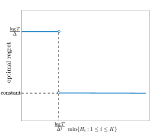
Figure 13: Phase transition in $K$-armed bandits with offline data when $\Delta=\Omega(T^{-\frac{1}{2}})$

There are three key differences between the $K$-armed bandit with offline data and the OPOD problem considered in this paper. First, in the $K$-armed bandit, the phase transition of the optimal regret only occur when the amount of offline data for each arm exceeds the threshold $\Theta(\frac{\log T}{\Delta^{2}})$; in other words, the offline data need to be balanced among different arms. By contrast, in the OPOD problem, even when there is only one historical price, i.e., $\sigma=0$, the optimal regret rate can drop from $\widetilde{\Theta}(\sqrt{T})$ to $\widetilde{\Theta}(\frac{\log T}{\delta^{2}})$ as the amount of offline data $n$ increases. The reason is that in $K$-armed bandit, different arms are independent, and the knowledge about the reward of one arm does not help to understand that of another. However, in dynamic pricing, the demands under different prices are connected with each other by the parametric assumption of the linear demand function. Therefore, knowing even one point at the demand curve can lead to a significant decrease in the optimal regret rate (see our Corollary 3.5 when $n=\infty$, or the incumbent price setting in Keskin and Zeevi 2014). Second, in the $K$-armed bandit, the optimal regret rate only shows two phases. In the first phase when the amount of the offline data is small, i.e., $\min\{H_{i}:i\in[K]\}=O(\frac{\log T}{\Delta^{2}})$, the optimal regret is always $\Theta(\frac{\log T}{\Delta})$ and the offline data do not help to reduce the optimal regret. In the second phase when the amount of the offline data is large, i.e., $\min\{H_{i}:i\in[K]\}=\Omega(\frac{\log T}{\Delta^{2}})$, the optimal regret becomes a constant. In the OPOD problem, however, the optimal regret gradually changes as the size of the offline data increases, experiencing different phase transitions depending on the magnitude of $\sigma$ and $\delta$. Third, under the so-called “well-separated” condition in bandits, where the sub-optimality gap $\Delta$ is a constant independent of $T$, the $K$-armed bandit exhibits weak phase transition in the sense that the drop of the optimal regret rate is within $\log T$. By comparison, under our well-separated condition , i.e., $\delta$ is a constant independent of $T$, the OPOD problem shows strong phase transitions in the sense that the drops of the optimal regret rate in multiple phases are measured in $T^{\kappa}$ for some $\kappa>0$, which are much more significant even if we ignore the logarithmic factor.

Appendix H. Tables in Sections 3 and 4

Table 3: Regret upper bound in Theorem 3.1 for the single-historical-price setting

Case 1: $\delta\gtrsim T^{-\frac{1}{4}}(\log T)^{\frac{1}{2}}$
offline sample size	$0\leq n\lesssim\frac{\sqrt{T}\log T}{\delta^{2}}$	$\frac{\sqrt{T}\log T}{\delta^{2}}\lesssim n\lesssim T$	$n\gtrsim T$
upper bound	$\mathcal{O}(\sqrt{T}\log T)$	$\mathcal{O}(\frac{T(\log T)^{2}}{n\delta^{2}})$	$\mathcal{O}(\frac{(\log T)^{2}}{\delta^{2}})$
Case 2: $\delta\lesssim T^{-\frac{1}{4}}(\log T)^{\frac{1}{2}}$
offline sample size	$n\geq 0$
upper bound	$\mathcal{O}(\sqrt{T}\log T)$

Table 4: Regret lower bound in Theorem 3.3 for the single-historical-price setting

Case 1: $\delta\gtrsim T^{-\frac{1}{4}}$
offline sample size	$0<n\lesssim\frac{\sqrt{T}}{\delta^{2}}$	$\frac{\sqrt{T}}{\delta^{2}}\lesssim n\lesssim T$	$n\gtrsim T$
lower bound	$\Omega(\sqrt{T})$	$\Omega(\frac{T}{n\delta^{2}}\vee\log T)$	$\Omega(\frac{1}{\delta^{2}}\vee\log T)$
Case 2: $T^{-\frac{1}{4}}(\log T)^{-\frac{1}{2}}\lesssim\delta\lesssim T^{-\frac{1}{4}}$
offline sample size	$n>0$
lower bound	$\Omega(T\delta^{2})$
Case 3: $\delta\lesssim T^{-\frac{1}{4}}(\log T)^{-\frac{1}{2}}$
offline sample size	$n>0$
lower bound	$\Omega(\frac{\sqrt{T}}{\log T})$

Table 5: Regret upper bound in Theorem 4.1 for the multiple-historical-price setting

Case 1: $\delta\gtrsim T^{-\frac{1}{4}}(\log T)^{\frac{1}{2}}$ and $\sigma\lesssim\delta$
offline sample size	$0\leq n\lesssim\frac{\sqrt{T}\log T}{\delta^{2}}$	$\frac{\sqrt{T}\log T}{\delta^{2}}\lesssim n\lesssim T$	$T\lesssim n\lesssim\frac{T\delta^{2}}{\sigma^{2}}$	$n\gtrsim\frac{T\delta^{2}}{\sigma^{2}}$
upper bound	$\mathcal{O}(\sqrt{T}\log T)$	$\mathcal{O}(\frac{T(\log T)^{2}}{n\delta^{2}})$	$\mathcal{O}(\frac{(\log T)^{2}}{\delta^{2}})$	$\mathcal{O}(\frac{T(\log T)^{2}}{n\sigma^{2}}+1)$
Case 2: $\delta\gtrsim T^{-\frac{1}{4}}(\log T)^{\frac{1}{2}}$ and $\sigma\gtrsim\delta$
offline sample size	$0\leq n\lesssim\frac{\sqrt{T}\log T}{\sigma^{2}}$		$n\gtrsim\frac{\sqrt{T}\log T}{\sigma^{2}}$
upper bound	$\mathcal{O}(\sqrt{T}\log T)$		$\mathcal{O}(\frac{T(\log T)^{2}}{n\sigma^{2}}+1)$
Case 3: $\delta\lesssim T^{-\frac{1}{4}}(\log T)^{\frac{1}{2}}$
offline sample size	$0\leq n\lesssim\frac{\sqrt{T}\log T}{\sigma^{2}}$	$\frac{\sqrt{T}\log T}{\sigma^{2}}\lesssim n\lesssim\frac{(\log T)^{2}}{\sigma^{2}\delta^{2}}$	$n\gtrsim\frac{(\log T)^{2}}{\sigma^{2}\delta^{2}}$
upper bound	$\mathcal{O}(\sqrt{T}\log T)$	$\mathcal{O}(T\delta^{2}+1)$	$\mathcal{O}(\frac{T(\log T)^{2}}{n\sigma^{2}}+1)$

Table 6: Regret lower bound in Theorem 4.3 for the multiple-historical-price setting

Case 1: $\delta\gtrsim T^{-\frac{1}{4}}(\log T)^{\frac{1}{2}}$ and $\sigma\lesssim\delta$
offline sample size	$0\leq n\lesssim\frac{\sqrt{T}\log T}{\delta^{2}}$	$\frac{\sqrt{T}\log T}{\delta^{2}}\lesssim n\lesssim T$	$T\lesssim n\lesssim\frac{T\delta^{2}}{\sigma^{2}}$	$n\gtrsim\frac{T\delta^{2}}{\sigma^{2}}$
lower bound	$\Omega(\frac{\sqrt{T}}{\log T})$	$\Omega(\frac{T}{n\delta^{2}})$	$\Omega(\frac{1}{\delta^{2}})$	$\Omega(\frac{T}{n\sigma^{2}})$
Case 2: $\delta\gtrsim T^{-\frac{1}{4}}(\log T)^{\frac{1}{2}}$ and $\sigma\gtrsim\delta$
offline sample size	$0\leq n\lesssim\frac{\sqrt{T}\log T}{\sigma^{2}}$		$n\gtrsim\frac{\sqrt{T}\log T}{\sigma^{2}}$
lower bound	$\Omega(\frac{\sqrt{T}}{\log T})$		$\Omega(\frac{T}{n\sigma^{2}})$
Case 3: $T^{-\frac{1}{4}}(\log T)^{-\frac{1}{2}}\lesssim\delta\lesssim T^{-\frac{1}{4}}(\log T)^{\frac{1}{2}}$
offline sample size	$0\leq n\lesssim\frac{1}{\sigma^{2}\delta^{2}}$		$n\gtrsim\frac{1}{\sigma^{2}\delta^{2}}$
lower bound	$\Omega(\frac{\sqrt{T}}{\log T})$		$\Omega(\frac{T}{n\sigma^{2}})$
Case 4: $\delta\lesssim T^{-\frac{1}{4}}(\log T)^{-\frac{1}{2}}$
offline sample size	$0\leq n\lesssim\frac{\sqrt{T}\log T}{\sigma^{2}}$	$\frac{\sqrt{T}\log T}{\sigma^{2}}\lesssim n\lesssim\frac{1}{\sigma^{2}\delta^{2}}$	$n\gtrsim\frac{1}{\sigma^{2}\delta^{2}}$
lower bound	$\Omega(\frac{\sqrt{T}}{\log T})$	$\Omega(T\delta^{2})$	$\Omega(\frac{T}{n\sigma^{2}})$

References

- Abbasi-Yadkori et al. (2011) Abbasi-Yadkori Y, Pál D, Szepesvári C (2011) Improved algorithms for linear stochastic bandits. Advances in Neural Information Processing Systems, 2312–2320.
- Agrawal et al. (2017) Agrawal S, Avadhanula V, Goyal V, Zeevi A (2017) Thompson sampling for the mnl-bandit. arXiv preprint arXiv:1706.00977 .
- Auer et al. (2002) Auer P, Cesa-Bianchi N, Fischer P (2002) Finite-time analysis of the multiarmed bandit problem. Machine learning 47(2-3):235–256.
- Ban and Keskin (2020) Ban GY, Keskin NB (2020) Personalized dynamic pricing with machine learning: High dimensional features and heterogeneous elasticity. Forthcoming, Management Science .
- Bastani et al. (2019) Bastani H, Simchi-Levi D, Zhu R (2019) Meta dynamic pricing: Learning across experiments. Available at SSRN 3334629 .
- Bouneffouf et al. (2019) Bouneffouf D, Parthasarathy S, Samulowitz H, Wistub M (2019) Optimal exploitation of clustering and history information in multi-armed bandit. arXiv preprint arXiv:1906.03979 .
- Broder and Rusmevichientong (2012) Broder J, Rusmevichientong P (2012) Dynamic pricing under a general parametric choice model. Operations Research 60(4):965–980.
- Cesa-Bianchi and Lugosi (2006) Cesa-Bianchi N, Lugosi G (2006) Prediction, learning, and games (Cambridge university press).
- Correa et al. (2018) Correa JR, Dütting P, Fischer F, Schewior K (2018) Prophet inequalities for independent random variables from an unknown distribution. arXiv preprint arXiv:1811.06114 .
- Dani et al. (2008) Dani V, Hayes TP, Kakade SM (2008) Stochastic linear optimization under bandit feedback. Proceedings of the 21st Conference on Learning Theory.
- den Boer and Keskin (2017) den Boer A, Keskin NB (2017) Dynamic pricing with demand learning and reference effects. Available at SSRN 3092745 .
- den Boer (2014) den Boer AV (2014) Dynamic pricing with multiple products and partially specified demand distribution. Mathematics of operations research 39(3):863–888.
- den Boer (2015) den Boer AV (2015) Dynamic pricing and learning: historical origins, current research, and new directions. Surveys in operations research and management science 20(1):1–18.
- den Boer and Zwart (2013) den Boer AV, Zwart B (2013) Simultaneously learning and optimizing using controlled variance pricing. Management science 60(3):770–783.
- Domb (2000) Domb C (2000) Phase transitions and critical phenomena, volume 19 (Elsevier).
- Ferreira et al. (2018) Ferreira KJ, Simchi-Levi D, Wang H (2018) Online network revenue management using thompson sampling. Operations research 66(6):1586–1602.
- Filippi et al. (2010) Filippi S, Cappe O, Garivier A, Szepesvári C (2010) Parametric bandits: The generalized linear case. Advances in Neural Information Processing Systems, 586–594.
- Gill and Levit (2001) Gill R, Levit B (2001) Applications of the van trees inequality: a bayesian cramér-rao bound. Bernoulli 1:59.
- Gur and Momeni (2019) Gur Y, Momeni A (2019) Adaptive sequential experiments with unknown information flows. arXiv preprint arXiv:1907.00107 .
- Harrison et al. (2012) Harrison JM, Keskin NB, Zeevi A (2012) Bayesian dynamic pricing policies: Learning and earning under a binary prior distribution. Management Science 58(3):570–586.
- Hastie et al. (2005) Hastie T, Tibshirani R, Friedman J, Franklin J (2005) The elements of statistical learning: data mining, inference and prediction. The Mathematical Intelligencer 27(2):83–85.
- Hsu et al. (2019) Hsu CW, Kveton B, Meshi O, Martin M, Szepesvari C (2019) Empirical bayes regret minimization. arXiv preprint arXiv:1904.02664 .
- Keskin and Zeevi (2014) Keskin N, Zeevi A (2014) Dynamic pricing with an unknown demand model: Asymptotically optimal semi-myopic policies. Operations Research 62(5):1142–1167.
- Keskin and Zeevi (2016) Keskin NB, Zeevi A (2016) Chasing demand: Learning and earning in a changing environment. Mathematics of Operations Research 42(2):277–307.
- Lattimore and Szepesvári (2018) Lattimore T, Szepesvári C (2018) Bandit algorithms. preprint .
- Li et al. (2017) Li L, Lu Y, Zhou D (2017) Provably optimal algorithms for generalized linear contextual bandits. Proceedings of the 34th International Conference on Machine Learning-Volume 70, 2071–2080 (JMLR. org).
- Miao and Chao (2020) Miao S, Chao X (2020) Dynamic joint assortment and pricing optimization with demand learning. Manufacturing & Service Operations Management .
- Nambiar et al. (2019) Nambiar M, Simchi-Levi D, Wang H (2019) Dynamic learning and pricing with model misspecification. Management Science .
- Qiang and Bayati (2016) Qiang S, Bayati M (2016) Dynamic pricing with demand covariates. Available at SSRN 2765257 .
- Rusmevichientong and Tsitsiklis (2010) Rusmevichientong P, Tsitsiklis JN (2010) Linearly parameterized bandits. Mathematics of Operations Research 35(2):395–411.