A Fast Saddle-Point Dynamical System Approach to Robust Deep Learning111*This work was partially supported by NSF CAREER Grant (CNS#1845969#1845969\#1845969)

Yasaman Esfandiari Aditya Balu Keivan Ebrahimi Umesh Vaidya Nicola Elia Soumik Sarkar Iowa State University Clemson University University of Minnesota soumiks@iastate.edu
Abstract

Recent focus on robustness to adversarial attacks for deep neural networks produced a large variety of algorithms for training robust models. Most of the effective algorithms involve solving the min-max optimization problem for training robust models (min step) under worst-case attacks (max step). However, they often suffer from high computational cost from running several inner maximization iterations (to find an optimal attack) inside every outer minimization iteration. Therefore, it becomes difficult to readily apply such algorithms for moderate to large size real world data sets. To alleviate this, we explore the effectiveness of iterative descent-ascent algorithms where the maximization and minimization steps are executed in an alternate fashion to simultaneously obtain the worst-case attack and the corresponding robust model. Specifically, we propose a novel discrete-time dynamical system-based algorithm that aims to find the saddle point of a min-max optimization problem in the presence of uncertainties. Under the assumptions that the cost function is convex and uncertainties enter concavely in the robust learning problem, we analytically show that our algorithm converges asymptotically to the robust optimal solution under a general adversarial budget constraints as induced by psubscript𝑝\ell_{p} norm, for 1p1𝑝1\leq p\leq\infty. Based on our proposed analysis, we devise a fast robust training algorithm for deep neural networks. Although such training involves highly non-convex robust optimization problems, empirical results show that the algorithm can achieve significant robustness compared to other state-of-the-art robust models on benchmark data sets.

keywords:
Adversarial Training, Robust Deep Learning, Robust optimization
journal: Neural Networks

1 Introduction

The success of adversarial perturbations to input data for deep learning models poses a significant challenge for the machine learning community. The motivation for robustness against these adversaries stems from safety and life-critical applications of deep learning-based perception system such as self-driving cars, infrastructure assessment and security applications [1, 2, 3, 4]. While pure white-box attacks [2, 5, 6, 7, 8, 9, 10] (where an adversary has full knowledge of the machine learning model) could be difficult to execute in practice, researchers have shown strong transferability of attacks [11] that can still cause significant damage.

As attacks became more and more powerful, several defense strategies have also been proposed. A popular category of defense strategy is adversarial training, where adversarial examples are added to the training set followed by training the network using the augmented dataset [6, 8]. However, such methods seem to be quite sensitive to adversarial budget used for generating the adversarial examples as well as other training hyper-parameters. A more powerful and stable defense mechanism originates from the min-max robust optimization problem (𝒪𝒪{\cal RO}[12, 13, 14] by decoupling the minimization and maximization parts using the Danskin’s theorem [15]. Here, the inner maximization refers to finding the adversarial perturbation that would maximize the training loss. On the other hand, the outer minimization deals with minimization of the training loss for the perturbed inputs. The decoupling process leads to the class of algorithms where, at a training epoch, one can find the worst-case attacks concerning the current model. Then a model parameter update step is executed following the traditional training process using perturbed training set with the worst-case attacks. However, finding the worst-case perturbation for deep learning models is quite non-trivial and cannot be guaranteed primarily due to the highly non-convex nature of the cost surface and non-concave nature of adversarial perturbations. Typically, powerful attacks such as projected gradient descent (PGD) [14], trade off-inspired adversarial defense via surrogate-loss minimization (TRADES) [16], Free adversarial training [17], etc. are run in order to find the worst-case perturbations at every training epoch. However, it is observed empirically that the attacks with higher computational budgets seem to be more successful in approximating the worst-case perturbations, e.g., 20 step PGD is much stronger than a single step PGD. Therefore, it is usually quite expensive computationally to find a robust deep learning model with this algorithmic principle. Besides, there still remains a significant gap in the literature, in crafting theoretically sound algorithms for robust learning. There are only a few studies exploring the robust learning problem analytically. Fawzi et al. [18] first analyzes robustness of nonlinear classifiers in a general noise regime, Shaham et al. [19] proposed a framework to justify the performance of adversarial training theoretically, Zhang et al. [16] considered the trade off between robustness and accuracy, and the recent paper by Lin et al. [20] proposes gradient descent ascent approach to solve the robust learning problem. Additionally, Sinha et al. [21] proposed an algorithm for solving the adversarial training problem from a distributionally robust optimization lens for finding the worst-case adversary based on the Lagrangian formulation of the objective function.

In this paper, we introduce a new algorithm for adversarial training of deep neural networks, which is motivated by the 𝒪𝒪{\cal RO} problem. Traditionally, robust optimization problems are solved iteratively by alternative steps of ascent and descent for achieving the worst case attack and finding the corresponding robust model for the attack. Our proposed defense approach called the stochastic saddle point dynamical systems (SSDS) algorithm, follows this principle to devise a fast algorithm for robust learning. We first formulate the min-max 𝒪𝒪{\cal RO} problem that arises in adversarial training of deep neural networks (DNNs) and show analytically that under strictly-convex and strictly-concave assumption for the loss function and the adversarial perturbations in the robust learning problem, SSDS algorithm converges asymptotically to the robust optimal solution, the min-max saddle point, under a general adversarial budget constraints as induced by psubscript𝑝\ell_{p} norm, for 1p1𝑝1\leq p\leq\infty.

Unlike existing approaches, our proposed algorithm does not decouple the minimization and maximization problems involved in robust optimization. Instead, it attempts to solve both problems simultaneously by evolving both the model parameters and the adversarial perturbations through the training epochs. As we do not attempt to find the worst-case perturbations at every training epoch, we save significant computation overhead as compared to other methods such as PGD-training [14], TRADES  [16], and YOPO [22]. While there are recent efforts to mitigate the computational overhead by using random projections  [23] instead of finding the worst case attacks, our approach is fundamentally different as we still try to solve the coupled robust optimization problem (that includes finding the worst case perturbations) while reducing the computations overhead.

Contributions: Main contributions of this work are: (i) We propose a new Stochastic Saddle-point Dynamical Systems (SSDS) algorithm for robust learning that ensure satisfaction of the attack budget (induced by psubscript𝑝\ell_{p} norm, for 1p1𝑝1\leq p\leq\infty) asymptotically without hard projections; (ii) We analyze the convergence characteristics for the proposed SSDS algorithm under the strictly-convex assumption for the loss function and strictly-concave assumption for the adversarial perturbations in the robust learning problem; (iii) We propose a mini-batch variant of the SSDS algorithm to make it feasible for deep learning problems; (iv) Finally, we provide empirical results (based on CIFAR-10 [24] and other benchmark datasets) to show that the proposed approach is a computationally inexpensive way to train robust models for white- and black-box attacks in comparison with the state-of-the-art PGD and TRADES approaches. We also provide comparison with the stochastic gradient descent ascent algorithm (SGDA) [20] that can be treated as a baseline for our proposed approach.

2 Related Work

Due to space constraints and a large amount of recent progress made by the adversarial machine learning community, our discussion of related work is necessarily brief. Here, we attempt to discuss the most recent & relevant literature. We divide the section as: (1) adversarial attack/defense and (2) robust optimization.

Adversarial Attack and Defense: Initial evidence for vulnerability of deep classifiers to imperceptible adversarial perturbations was shown by Szegedy et al. [8]. Around the same time, Biggio et al. [2] showed that SVMs could malfunction in security-sensitive applications and proposed a regularization term in the classifiers. In the deep learning community, Goodfellow et al. [6] and Kurakin et al. [7] proposed the Fast Gradient Sign Method (FGSM) and its iterative variants as powerful attack strategies to fool deep learning models. adopting a similar notion, PGD [14] attacks are crafted by going through iterative steps of generating attacks (e.g. 777 and 101010 steps) to achieve more powerful adversaries. As the computational expenses associated with such attacks are significant, researchers have recently suggested different methods to mitigate that. Shafahi et al. [17] suggested using the gradients which is calculated for updating the model parameters to save computations and showed comparable results with state-of-the-art. Wong et al. [25] showed that comparably accurate models can be achieved in less time using FGSM along with several techniques from DAWNBench submissions [26] (e.g., random initialization) to improve the performance. Additionally, Zhang et al. [22] showed that by restricting most of the forward and back propagation within the first layer of the network during adversary updates, the computational time for achieving a robust model can be reduced. While these methods mainly focused on white box attacks, Papernot et al. [11] introduced the notion of black-box attacks where the adversary does not have complete knowledge of the learning model. Attacks can also be categorized into test-time [2] and train-time (also known as data poisoning) attacks [27], and targeted and non-targeted attacks [28]. In this paper, we only focus on test-time, non-targeted attacks. Apart from deep perception models such as Convolutional Neural Networks (CNN), researchers have also shown similar vulnerabilities of deep reinforcement learning (RL) models using similar philosophy [29, 30, 31, 32, 33]. The notion of adversarial robustness is additionally useful in other areas of machine learning such as image synthesis [34, 35].

Several defense approaches have been proposed in the literature, such as using denoising autoencoders-based Deep Contractive Networks [36], and defining a network robustness metric [37]. However, as discussed in the previous section, the most popular robust deep learning methods involve some form of adversarial training [38, 14, 6, 19, 16, 39]. Defensive distillation [40] is also another method of defense which showed fascinating results. However, Carlini and Wagner [5] could break such a defense mechanism by proposing multiple adversarial loss functions. Athalye et al. [41] further analyzed various defense approaches and demonstrated that most existing defenses could be beaten by approximating gradients over defensively trained models. Recently, Zhang and Wang [39] introduced Feature Scatter algorithm which increased the accuracy of robust models notably. This approach involves generating adversarial images through feature scattering in the latent space.

Robust Optimization: Shaham et al. [19] show that adversarial training of neural networks is, in fact, robustification of the network optimization, which we can exploit to increase the local stability of neural networks. Robust optimization has also been used in [42] to find an approximately optimal min-max solution that optimizes for non-convex objectives. This method is based on a reduction from robust optimization to stochastic optimization. Here a α𝛼\alpha-approximate stochastic oracle is given, and α𝛼\alpha-approximate robust optimization in a convexified solution space is obtained. Nonetheless, ideas from robust optimization (closely related to regularization in machine learning [43, 44]) for solving robust learning problems has not been explored sufficiently. Also, while there is recent work in robust optimization using continuous-time dynamical systems for the saddle point dynamics [45], it is deterministic, and its application to deep learning problems is not explored.

3 Problem Formulation

In this section, we first formally state the robust learning problem from a robust optimization point of view. Then we formulate the saddle-point dynamical system framework for solving robust learning problems. We consider a standard classification task under a data distribution 𝒟𝒟{\cal D} over the dataset I={I1,I2,,IN}𝐼superscript𝐼1superscript𝐼2superscript𝐼𝑁I=\{I^{1},I^{2},\cdots,I^{N}\}, where, Ii𝐑msuperscript𝐼𝑖superscript𝐑𝑚I^{i}\in\mathbf{R}^{m} with set of labels, y𝑦y. The loss function (e.g., cross-entropy loss) is denoted by L(I,y,w)𝐿𝐼𝑦𝑤L(I,y,w) with w𝐑n𝑤superscript𝐑𝑛w\in\mathbf{R}^{n} as the model parameters (decision variables). From a robust optimization (𝒪𝒪{\cal RO}) perspective [12, 13, 19, 45], robust learning can be written as

𝒪:=assign𝒪absent\displaystyle{\cal RO}:= minw𝔼(I,y)𝒟[maxu𝒰L(I+u,y,w)]subscript𝑤subscript𝔼similar-to𝐼𝑦𝒟delimited-[]𝑢𝒰𝐿𝐼𝑢𝑦𝑤\displaystyle\min_{w}\;\mathbb{E}_{(I,y)\sim{\cal D}}\;\Big{[}\underset{u\in{\cal U}}{\max}\;\;L(I+u,y,w)\Big{]}\; (1)

where, the loss function L𝐿L is also a function of additive perturbation or uncertainty u𝑢u (constrained by uncertainty set 𝒰𝒰\cal U) to the input.

We approximate the expected loss using the standard empirical risk minimization for a finite number of i.i.d training samples, Iifori{1,2,N}superscript𝐼𝑖for𝑖12𝑁I^{i}\ \text{for}\ i\in\{1,2,\cdots N\}. We consider uisuperscript𝑢𝑖u^{i} as the corresponding uncertainty for the data point Iisuperscript𝐼𝑖I^{i}. Hence, 𝒪𝒪{\cal RO} problem (Eq. 1) can be written as

𝒪:=assign𝒪absent\displaystyle{\cal RO}:= minwi=1Nmaxui𝒰iL(Ii+ui,yi,w)subscript𝑤superscriptsubscript𝑖1𝑁superscript𝑢𝑖superscript𝒰𝑖𝐿superscript𝐼𝑖superscript𝑢𝑖superscript𝑦𝑖𝑤\displaystyle\min_{w}\textstyle\sum_{i=1}^{N}\underset{u^{i}\in{\cal U}^{i}}{\max}\;L(I^{i}+u^{i},y^{i},w)\; (2)

The fundamental assumption in 𝒪𝒪{\cal RO} is that the uncertainty variables reside within the uncertainty sets

𝒰i:={ui𝐑m:hi(ui)0},i=1,,N,formulae-sequenceassignsuperscript𝒰𝑖conditional-setsuperscript𝑢𝑖superscript𝐑𝑚superscript𝑖superscript𝑢𝑖0𝑖1𝑁\displaystyle{\cal U}^{i}:=\{u^{i}\in\mathbf{R}^{m}:h^{i}(u^{i})\leq 0\},\;i=1,\ldots,N\;, (3)

where the hisuperscript𝑖h^{i} functions representing the uncertainty sets are typically assumed to be convex functions such as norm-bound budgets. The goal here is to obtain model parameters, w𝑤w, (e.g., weights and biases for neural networks) that are robust for all possible uncertainty parameter realizations within the uncertainty sets.

We assume that the 𝒪𝒪{\cal RO} problem (Eq. 1) has at least one robust feasible solution. Then we rewrite Eq. 1 in an epigraph form [46].

𝒪:=minw,ttassign𝒪subscript𝑤𝑡𝑡\displaystyle\quad\quad\quad{\cal RO}:=\min_{w,t}\;t
s.t i=1Nmaxui𝒰iL(Ii+ui,yi,w)t0superscriptsubscript𝑖1𝑁superscript𝑢𝑖superscript𝒰𝑖𝐿superscript𝐼𝑖superscript𝑢𝑖superscript𝑦𝑖𝑤𝑡0\displaystyle\sum_{i=1}^{N}\underset{u^{i}\in{\cal U}^{i}}{\max}L(I^{i}+u^{i},y^{i},w)-t\leq 0 (4)

This is an equivalent, albeit more convenient form for our framework, where t𝑡t is being added to the vector of model parameters as an auxiliary decision variable.

We define a Lagrangian multiplier λ0𝜆0\lambda\geq 0 and the vector of model parameters as x:=(w,t)assign𝑥𝑤𝑡x:=(w,t). We can write Eq. 3 as

minx=(w,t)maxλ0{t+λ(i=1Nmaxui𝒰iL(Ii+ui,yi,w)t)}𝑥𝑤𝑡𝜆0𝑡𝜆superscriptsubscript𝑖1𝑁superscript𝑢𝑖superscript𝒰𝑖𝐿superscript𝐼𝑖superscript𝑢𝑖superscript𝑦𝑖𝑤𝑡\displaystyle\underset{x=(w,t)}{\min}\;\underset{\lambda\geq 0}{\max}\;\Big{\{}t+\lambda\;\big{(}\sum_{i=1}^{N}\underset{u^{i}\in{\cal U}^{i}}{\max}\;L(I^{i}+u^{i},y^{i},w)-t\big{)}\Big{\}}\;

Then the total Lagrangian can be written as

(x,λ,u,v):=assign𝑥𝜆𝑢𝑣absent\displaystyle{\cal L}(x,\lambda,u,v):= t+λ(i=1N(L(Ii+ui,yi,w)\displaystyle\;t+\lambda\;\Big{(}\textstyle\sum_{i=1}^{N}\big{(}L(I^{i}+u^{i},y^{i},w)
vihi(ui))t)\displaystyle\;-v^{i}\;h^{i}(u^{i})\big{)}-t\Big{)}\; (5)

where the set {vi}superscript𝑣𝑖\{v^{i}\} are the Lagrangian multipliers for the inner maximization problem. Typically, loss function in an 𝒪𝒪{\cal RO} framework is considered to be a function of just the model parameters, not the uncertainty. Therefore, we formulate the algorithm with Lagrangian multipliers that ensure satisfaction of the attack budget asymptotically without hard projections.

Remark 1.

The ability to solve 𝒪𝒪{\cal RO} with general budget constraints without involving hard projection is advantageous from a computational perspective, as imposing hard projection may involve solving an optimization problem in itself.

Derivation of the Lagrangian function along with the definition and properties of the saddle and KKT point of 𝒪𝒪{\cal RO} problem can be found in the supplementary material.

4 Stochastic Saddle-Point Dynamical System Algorithm

Based on the problem setup laid out in the previous section, we now propose the stochastic saddle-point dynamical system (SSDS) algorithm for robust learning. We then introduce the mini-batch variant of the SSDS algorithm conducive to deep learning. Additionally, we also state the stochastic gradient descent ascent (SGDA) algorithm (Lin et al. [20]), which can be considered as a simplified baseline for the proposed SSDS algorithm.

4.1 Algorithm Formulation

In the previous section, we provided the total Lagrangian for obtaining the saddle and KKT point of 𝒪𝒪{\cal RO} problem. While that is sufficient to understand the saddle point dynamics of the 𝒪𝒪{\cal RO} problem, the implementation for deep learning problems necessitates the formulation of a stochastic discrete-time saddle point dynamical system to find the saddle point of the Lagrangian function. Based on the epigraph form of the optimization problem (Eq. 3), we define x:=(t,w),f(x):=t,g(x,u,ξ):=L(Iξ+uξ,y,w)tformulae-sequenceassign𝑥𝑡𝑤formulae-sequenceassign𝑓𝑥𝑡assign𝑔𝑥𝑢𝜉𝐿superscript𝐼𝜉superscript𝑢𝜉𝑦𝑤𝑡x:=(t,w),\ f(x):=t,\ g(x,u,\xi):=L(I^{\xi}+u^{\xi},y,w)-t, where ξ{1,,N}𝜉1𝑁\xi\in\{1,\ldots,N\} is a random variable modeling the process for randomly selecting a data point out of N𝑁N possible samples.

With these notations, we propose the following update rules for the parameters:

xk+1=xkαk(xf(xk)+λkxg(xk,uk,ξk)),subscript𝑥𝑘1subscript𝑥𝑘subscript𝛼𝑘subscript𝑥𝑓subscript𝑥𝑘subscript𝜆𝑘subscript𝑥𝑔subscript𝑥𝑘subscript𝑢𝑘subscript𝜉𝑘\displaystyle x_{k+1}=x_{k}-\alpha_{k}(\partial_{x}f(x_{k})+\lambda_{k}\partial_{x}g(x_{k},u_{k},\xi_{k}))\;, (6)
λk+1=[λk+αk(g(xk,uk,ξk)i=1Nvkihi(uki))]+,subscript𝜆𝑘1subscriptdelimited-[]subscript𝜆𝑘subscript𝛼𝑘𝑔subscript𝑥𝑘subscript𝑢𝑘subscript𝜉𝑘superscriptsubscript𝑖1𝑁superscriptsubscript𝑣𝑘𝑖superscript𝑖subscriptsuperscript𝑢𝑖𝑘\displaystyle\lambda_{k+1}=\big{[}\lambda_{k}+\alpha_{k}\big{(}g(x_{k},u_{k},\xi_{k})-\textstyle\sum_{i=1}^{N}v_{k}^{i}h^{i}(u^{i}_{k})\big{)}\big{]}_{+}\;, (7)
uk+1i=uki+αk(uig(xk,uk)vkiuihi(uki)),subscriptsuperscript𝑢𝑖𝑘1subscriptsuperscript𝑢𝑖𝑘subscript𝛼𝑘subscriptsuperscript𝑢𝑖𝑔subscript𝑥𝑘subscript𝑢𝑘superscriptsubscript𝑣𝑘𝑖subscriptsuperscript𝑢𝑖superscript𝑖subscriptsuperscript𝑢𝑖𝑘\displaystyle u^{i}_{k+1}=u^{i}_{k}+\alpha_{k}(\partial_{u^{i}}g(x_{k},u_{k})-v_{k}^{i}\partial_{u^{i}}h^{i}(u^{i}_{k}))\;, (8)
vk+1i=[vki+αkλkhi(uki)]+i=1,,N.formulae-sequencesubscriptsuperscript𝑣𝑖𝑘1subscriptdelimited-[]superscriptsubscript𝑣𝑘𝑖subscript𝛼𝑘subscript𝜆𝑘superscript𝑖subscriptsuperscript𝑢𝑖𝑘𝑖1𝑁\displaystyle v^{i}_{k+1}=[v_{k}^{i}+\alpha_{k}\lambda_{k}h^{i}(u^{i}_{k})]_{+}\;\;i=1,\ldots,N. (9)

where, []+subscriptdelimited-[][\cdot]_{+} is positive projection, ξksubscript𝜉𝑘\xi_{k} is assumed to be an independent and identically distributed random process and αksubscript𝛼𝑘\alpha_{k} is the adaptive step-size with the following characteristics

αk=γkT(zk)2,withγk>0,formulae-sequencesubscript𝛼𝑘subscript𝛾𝑘subscriptnorm𝑇subscript𝑧𝑘2withsubscript𝛾𝑘0\displaystyle\alpha_{k}=\frac{\gamma_{k}}{\|T(z_{k})\|_{2}}\;,{\rm with}\;\;\gamma_{k}>0\;,
k=1γk=,k=1γk2<.formulae-sequencesuperscriptsubscript𝑘1subscript𝛾𝑘superscriptsubscript𝑘1superscriptsubscript𝛾𝑘2\displaystyle\sum_{k=1}^{\infty}\gamma_{k}=\infty\;,\;\textstyle\sum_{k=1}^{\infty}\gamma_{k}^{2}<\infty\;. (10)

The following assumptions are made on f𝑓f, g𝑔g and hisuperscript𝑖h^{i} s. Note that the weights x𝑥x is updated using the loss function information for a randomly selected sample Iξsuperscript𝐼𝜉I^{\xi}. However, the uncertainty variables uisuperscript𝑢𝑖u^{i} and associated multipliers visuperscript𝑣𝑖v^{i} are updated corresponding to all samples.

Assumption 1.

We assume that f(x)𝑓𝑥f(x) is convex in x𝑥x and each hi(ui)superscript𝑖superscript𝑢𝑖h^{i}(u^{i}) is convex in uisuperscript𝑢𝑖u^{i}. Moreover, g(x,u,ξ)𝑔𝑥𝑢𝜉g(x,u,\xi) is convex in x𝑥x and is strictly concave in u𝑢u for any fixed value of  ξ𝜉\xi.

Remark 2.

Clearly, the assumptions of strict convexity of f𝑓f and concavity of g𝑔g are not satisfied in the DNN setting. However, the strict convexity and strict concavity assumptions could be relaxed with weaker convergence results than the one reported below.

The following theorem is the main result for asymptotic convergence of the discrete-time saddle point algorithm with diminishing step-size. We show that the update rules in (6)-(9) lead to convergence to the KKT point (equivalent to the saddle point as specified in the supplementary material) of the 𝒪𝒪{\cal RO} problem.

Theorem 2.

Let Assumption 1 hold and we also assume that λ>0superscript𝜆0\lambda^{\star}>0 where λsuperscript𝜆\lambda^{\star} is the saddle point of the Lagrangian (for λ𝜆\lambda in Eq.5), then, following is true for the SSDS algorithm with adaptive step-size αksubscript𝛼𝑘\alpha_{k} satisfying Eq. 4.1.

limk𝔼ξ0k[xk]=x,subscript𝑘subscript𝔼superscriptsubscript𝜉0𝑘delimited-[]subscript𝑥𝑘superscript𝑥\displaystyle\lim_{k\to\infty}\mathbb{E}_{\xi_{0}^{k}}[x_{k}]=x^{\star}, limk𝔼ξ0k[uk]=u,subscript𝑘subscript𝔼superscriptsubscript𝜉0𝑘delimited-[]subscript𝑢𝑘superscript𝑢\displaystyle\lim_{k\to\infty}\mathbb{E}_{\xi_{0}^{k}}[u_{k}]=u^{\star}\;, (11)
whereξ0kwheresuperscriptsubscript𝜉0𝑘\displaystyle\text{where}\quad\xi_{0}^{k} ={ξ0,,ξk}.absentsubscript𝜉0subscript𝜉𝑘\displaystyle=\{\xi_{0},\ldots,\xi_{k}\}.\vspace{-20pt}
Proof.

The proof of the theorem is provided in the supplementary material.

The basic idea behind the convergence proof relies on proving the existence of saddle point (x,λ,v,u)superscript𝑥superscript𝜆superscript𝑣superscript𝑢(x^{\star},\lambda^{\star},v^{\star},u^{\star}) for the Lagrangian function, \cal L

(x,λ,u,v):=f(x)+λassign𝑥𝜆𝑢𝑣𝑓𝑥𝜆\displaystyle{\cal L}(x,\lambda,u,v):=f(x)+\lambda (12)
(g(x,u,ξ)i=1Nvihi(ui))𝑔𝑥𝑢𝜉superscriptsubscript𝑖1𝑁superscript𝑣𝑖superscript𝑖superscript𝑢𝑖\displaystyle\left(g(x,u,\xi)-\sum_{i=1}^{N}v^{i}h^{i}(u^{i})\right) (13)

satisfying the following inequalities for all realization of the random variable ξ𝜉\xi

(x,λ,v,u,ξ)(x,λ,v,u,ξ)(x,λ,v,u,ξ)superscript𝑥𝜆superscript𝑣𝑢𝜉superscript𝑥superscript𝜆superscript𝑣superscript𝑢𝜉𝑥superscript𝜆𝑣superscript𝑢𝜉{\cal L}(x^{\star},\lambda,v^{\star},u,\xi)\leq{\cal L}(x^{\star},\lambda^{\star},v^{\star},u^{\star},\xi)\leq{\cal L}(x,\lambda^{\star},v,u^{\star},\xi)

It is important to emphasize that although the function f𝑓f, g𝑔g, and hh are assumed to be convex with respect to x𝑥x and concave with respect to u𝑢u (Assumption 1), the Lagrangian function, {\cal L}, is not jointly concave with respect to (u,λ)𝑢𝜆(u,\lambda). The lack of joint concavity makes the saddle point proof nontrivial and different from the saddle point problem for a general min-max optimization problem (Lin et al. [20]). The existence of saddle point for min-max optimization problem under convexity-concavity assumption is a standard result in convex optimization and is at the heart of the convergence proof of the stochastic gradient descent-ascent algorithm.

Remark 3.

Although the stability is not shown in this paper, we observe in practice that the dynamics without λ𝜆\lambda in the v𝑣v-update (Eq.9) works for both active and inactive constraints (whether λsuperscript𝜆\lambda^{\star} is positive or zero) of the 𝒪𝒪{\cal RO} problem and converges to the KKT point. Therefore, λ𝜆\lambda can be removed from v𝑣v-update in practice for solving the 𝒪𝒪{\cal RO} problem.

Algorithm 1 Mini-batch SSDS algorithm
1:  Input: ε𝜀\varepsilon, lr, p𝑝p, C1subscript𝐶1C_{1}, C2subscript𝐶2C_{2}
2:  Initialization: λ0subscript𝜆0\lambda_{0}, α0subscript𝛼0\alpha_{0},w0subscript𝑤0w_{0}, t0subscript𝑡0t_{0},u0subscript𝑢0u_{0}, v0subscript𝑣0v_{0}
3:  for k{1,,K}𝑘1𝐾k\in\{1,...,K\} do
4:     distribute mini-batches as m={m0,m1,..,mn}m=\{m_{0},m_{1},..,m_{n}\}
5:     wkm0=wksuperscriptsubscript𝑤𝑘subscript𝑚0subscript𝑤𝑘w_{k}^{m_{0}}=w_{k}
6:     λkm0=λksuperscriptsubscript𝜆𝑘subscript𝑚0subscript𝜆𝑘\lambda_{k}^{m_{0}}=\lambda_{k}
7:     for mj{m0,m1,,mn}subscript𝑚𝑗subscript𝑚0subscript𝑚1subscript𝑚𝑛m_{j}\in\{m_{0},m_{1},...,m_{n}\} do
8:        wk=wkjmjL(Ij+ukj,yj,wkj)subscriptsubscript𝑤𝑘subscriptsubscript𝑤𝑘subscript𝑗subscript𝑚𝑗𝐿superscript𝐼𝑗superscriptsubscript𝑢𝑘𝑗superscript𝑦𝑗superscriptsubscript𝑤𝑘𝑗\partial_{w_{k}}=\partial_{w_{k}}\sum_{j\in m_{j}}L(I^{j}+u_{k}^{j},y^{j},w_{k}^{j})
9:        wkmj+1=wkmjlrλk(wk)superscriptsubscript𝑤𝑘subscript𝑚𝑗1superscriptsubscript𝑤𝑘subscript𝑚𝑗𝑙𝑟subscript𝜆𝑘subscriptsubscript𝑤𝑘w_{k}^{m_{j+1}}=w_{k}^{m_{j}}-lr\;\lambda_{k}(\partial_{w_{k}})
10:     end for
11:     tk+1=tk+αk(λk1)subscript𝑡𝑘1subscript𝑡𝑘subscript𝛼𝑘subscript𝜆𝑘1t_{k+1}=t_{k}+\alpha_{k}(\lambda_{k}-1)
12:     vk+1mj=vkmj+αk(ukmjε)superscriptsubscript𝑣𝑘1subscript𝑚𝑗superscriptsubscript𝑣𝑘subscript𝑚𝑗subscript𝛼𝑘subscriptnormsuperscriptsubscript𝑢𝑘subscript𝑚𝑗𝜀v_{k+1}^{m_{j}}=v_{k}^{m_{j}}+\alpha_{k}(\|u_{k}^{m_{j}}\|_{\infty}-\varepsilon)
13:     uk=ukL(Imj+ukmj,ymj,wkmj)subscriptsubscript𝑢𝑘subscriptsubscript𝑢𝑘𝐿superscript𝐼subscript𝑚𝑗superscriptsubscript𝑢𝑘subscript𝑚𝑗superscript𝑦subscript𝑚𝑗superscriptsubscript𝑤𝑘subscript𝑚𝑗\partial_{u_{k}}=\partial_{u_{k}}L(I^{m_{j}}+u_{k}^{m_{j}},y^{m_{j}},w_{k}^{m_{j}})
14:     uk+1mj=ukmj+αk(ukC1vkmjsign(ukmj))superscriptsubscript𝑢𝑘1subscript𝑚𝑗superscriptsubscript𝑢𝑘subscript𝑚𝑗subscript𝛼𝑘subscriptsubscript𝑢𝑘subscript𝐶1superscriptsubscript𝑣𝑘subscript𝑚𝑗signsuperscriptsubscript𝑢𝑘subscript𝑚𝑗u_{k+1}^{m_{j}}=u_{k}^{m_{j}}+\alpha_{k}(\partial_{u_{k}}-C_{1}\;v_{k}^{m_{j}}\operatorname*{sign}(u_{k}^{m_{j}}))
15:     for jmj𝑗subscript𝑚𝑗j\in m_{j} do
16:        Bj=(ukjε)superscript𝐵𝑗subscriptnormsuperscriptsubscript𝑢𝑘𝑗𝜀B^{j}=(\|u_{k}^{j}\|_{\infty}-\varepsilon)
17:        Uj=(L(Ij+ukj,yj,wkj)vkj)Bjsuperscript𝑈𝑗𝐿superscript𝐼𝑗superscriptsubscript𝑢𝑘𝑗superscript𝑦𝑗superscriptsubscript𝑤𝑘𝑗superscriptsubscript𝑣𝑘𝑗superscript𝐵𝑗U^{j}=\big{(}L(I^{j}+u_{k}^{j},y^{j},w_{k}^{j})-v_{k}^{j}\big{)}B^{j}
18:     end for
19:     U=jmjU(j)𝑈subscript𝑗subscript𝑚𝑗superscript𝑈𝑗U=\sum_{j\in m_{j}}U^{(j)}
20:     λk+1mj=λkmj+C2αk(Utk)superscriptsubscript𝜆𝑘1subscript𝑚𝑗superscriptsubscript𝜆𝑘subscript𝑚𝑗subscript𝐶2subscript𝛼𝑘𝑈subscript𝑡𝑘\lambda_{k+1}^{m_{j}}=\lambda_{k}^{m_{j}}+C_{2}\;\alpha_{k}\Big{(}U-t_{k}\Big{)}
21:     wk=wkmnsubscript𝑤𝑘superscriptsubscript𝑤𝑘subscript𝑚𝑛w_{k}=w_{k}^{m_{n}}
22:     λk=λk+1mnsubscript𝜆𝑘superscriptsubscript𝜆𝑘1subscript𝑚𝑛\lambda_{k}=\lambda_{k+1}^{m_{n}}
23:     αk+1=αkekpsubscript𝛼𝑘1subscript𝛼𝑘superscript𝑒𝑘p\alpha_{k+1}=\alpha_{k}e^{-k\textit{p}}
24:  end for

4.2 Mini-batch Implementation of SSDS Algorithm

In an attempt to use the proposed approach for robust training of DNNs, we propose a mini-batch variant of the SSDS algorithm to achieve a more stable convergence. As stated above, the SSDS algorithm involves the decision variable x:=(t,w)assign𝑥𝑡𝑤x:=(t,w), where the set {w}𝑤\{w\} is the parameters of DNN. For simplicity of implementation, we first separate the update rule for x𝑥x, described in Eq. 6. In other words, we split the updates of w𝑤w and t𝑡t that also enables us to use standard learning rates (denoted by lr) for the w𝑤w updates. For the updates of t𝑡t and other SSDS variables, such as λ𝜆\lambda, u𝑢u and v𝑣v, we use a diminishing step-size αksubscript𝛼𝑘\alpha_{k}. However, we refrain from applying the diminishing step-size described in (Eq. 4.1) due to the sheer complexity involved in taking the norm of the parameters for a large-scale neural network. Instead, we use an exponentially decaying diminishing step-size, αk+1=αkekpsubscript𝛼𝑘1subscript𝛼𝑘superscript𝑒𝑘p\alpha_{k+1}=\alpha_{k}e^{-k\textit{p}}, where p𝑝p is the decay rate for exponentially diminishing step-size and k𝑘k is the epoch number. Note that the updates of u𝑢u and λ𝜆\lambda can experience scaling issues depending on the values of the gradients and variable vksubscript𝑣𝑘v_{k}. Therefore, we add two scaling factors C1subscript𝐶1C_{1} and C2subscript𝐶2C_{2} in the update rules of u𝑢u and λ𝜆\lambda to bring different terms of the update laws to the same scale. For a given data set and model architecture, we find appropriate values by a few trial and error steps. Due to the separation of the updates, another small departure in our implementation from the prescribed algorithm is - while we perform w𝑤w updates for every mini-batch (mjsubscript𝑚𝑗m_{j} refers to the jthsuperscript𝑗𝑡j^{th} mini-batch of kthsuperscript𝑘𝑡k^{th} epoch), we update other parameters once every epoch. Also, in the original formulation, we continuously update u𝑢u corresponding to all the images while the w𝑤w is updated using the gradient information of the loss function evaluated at randomly selected images. In the algorithm implementation, however, u𝑢u is also updated only corresponding to the randomly selected images based on which the network weights are updated. This approach helps in reducing computation for large training sets.

Based on the above setup, we present the mini-batch SSDS algorithm (Algorithm 1). We can also craft attacks using this. To do that, we run iterative updates of the perturbations u𝑢u given a test sample along with its corresponding Lagrangian multiplier v𝑣v, keeping the model {w}superscript𝑤\{w^{\star}\} and λsuperscript𝜆\lambda^{*} fixed. We discuss the attack algorithm in the supplementary material.

4.3 Stochastic Gradient Descent Ascent (SGDA)

In order to study the effectiveness of the Lagrangian formulation to solve the robust optimization problem, we consider the baseline SGDA algorithm (Lin et al. [20]), which is essentially a simplification of the proposed SSDS algorithm as discussed below. We provide a mini-batch variant of the SGDA algorithm in Algorithm 2 to make it applicable in the deep learning setting. Comparing these two algorithms, we can readily see that algorithm 2 is a special case of algorithm 1 where the Lagrangian multipliers (λ𝜆\lambda and v𝑣v) are removed. Note, an important analytical advantage of the robust optimization-based formulation involving the Lagrangian function (Eq. 5) is that it allows us to incorporate general convex budget constraints (Eq. 3) on the adversary without involving complicated projection operations. In particular, with the Lagrangian multipliers λ𝜆\lambda and visuperscript𝑣𝑖v^{i}, we can ensure that the budget constraints are met asymptotically. It is important to emphasize that the use of projection operator to impose general convex budget constraints involves solving an optimization problem in itself and hence it could considerably increase the computational time. However, when the budget constraints are simple such as subscript\ell_{\infty} norm constraints, the projection operation is straight forward. For such cases, gradient descent ascent algorithm can be utilized for adversarial training without involving the multipliers.
Algorithm 2 Mini-batch SGDA algorithm
1:  Input: ε𝜀\varepsilon, lr, p𝑝p
2:  Initialization: α0subscript𝛼0\alpha_{0},w0subscript𝑤0w_{0},u0subscript𝑢0u_{0}
3:  for k{1,,K}𝑘1𝐾k\in\{1,...,K\} do
4:     distribute mini-batches as m={m0,m1,..,mn}m=\{m_{0},m_{1},..,m_{n}\}
5:     wk(m0)=wksuperscriptsubscript𝑤𝑘subscript𝑚0subscript𝑤𝑘w_{k}^{(m_{0})}=w_{k}
6:     for mj{m0,m1,,mn}subscript𝑚𝑗subscript𝑚0subscript𝑚1subscript𝑚𝑛m_{j}\in\{m_{0},m_{1},...,m_{n}\} do
7:        wk=wkjmjL(Ij+ukj,yj,wkj)subscriptsubscript𝑤𝑘subscriptsubscript𝑤𝑘subscript𝑗subscript𝑚𝑗𝐿superscript𝐼𝑗superscriptsubscript𝑢𝑘𝑗superscript𝑦𝑗superscriptsubscript𝑤𝑘𝑗\partial_{w_{k}}=\partial_{w_{k}}\sum_{j\in m_{j}}L(I^{j}+u_{k}^{j},y^{j},w_{k}^{j})
8:        wk(mj+1)=wk(mj)lr(wk)superscriptsubscript𝑤𝑘subscript𝑚𝑗1superscriptsubscript𝑤𝑘subscript𝑚𝑗𝑙𝑟subscriptsubscript𝑤𝑘w_{k}^{(m_{j+1})}=w_{k}^{(m_{j})}-lr\;(\partial_{w_{k}})
9:     end for
10:     uk+1mj=ukmj+αk(ukL(Imj+ukmj,ymj,wkmj)u_{k+1}^{m_{j}}=u_{k}^{m_{j}}+\alpha_{k}(\partial_{u_{k}}L(I^{m_{j}}+u_{k}^{m_{j}},y^{m_{j}},w_{k}^{m_{j}})
11:     wk=wkmnsubscript𝑤𝑘superscriptsubscript𝑤𝑘subscript𝑚𝑛w_{k}=w_{k}^{m_{n}}
12:     αk+1=αkekpsubscript𝛼𝑘1subscript𝛼𝑘superscript𝑒𝑘p\alpha_{k+1}=\alpha_{k}e^{-k\textit{p}}
13:  end for
Refer to caption
(a)
Refer to caption
(b)
Refer to caption
(c)
Refer to caption
(d)
Refer to caption
(e)
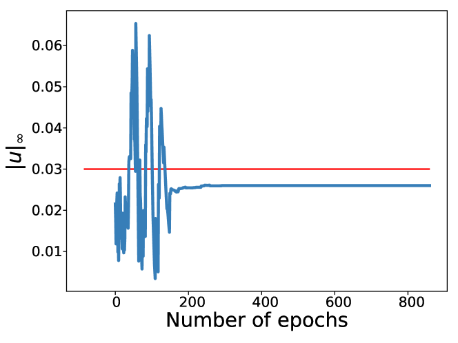
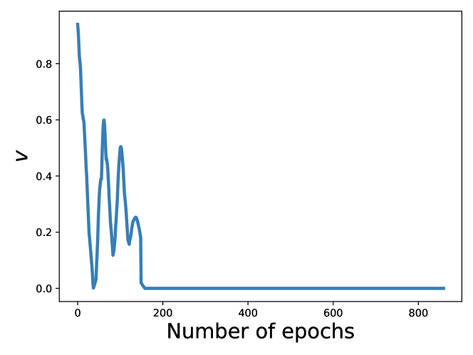
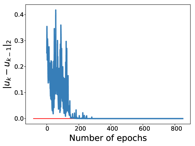
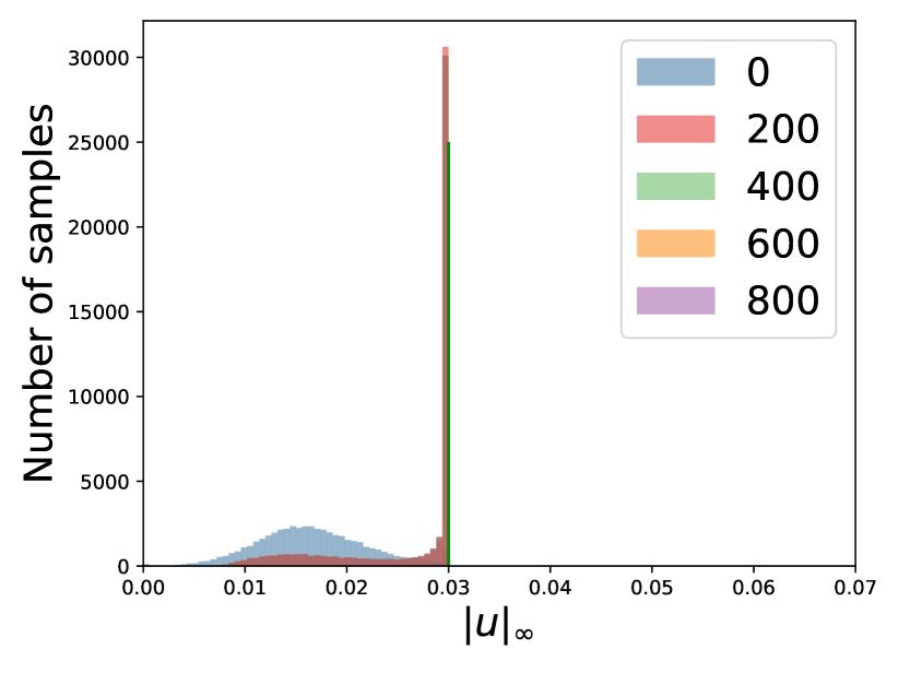
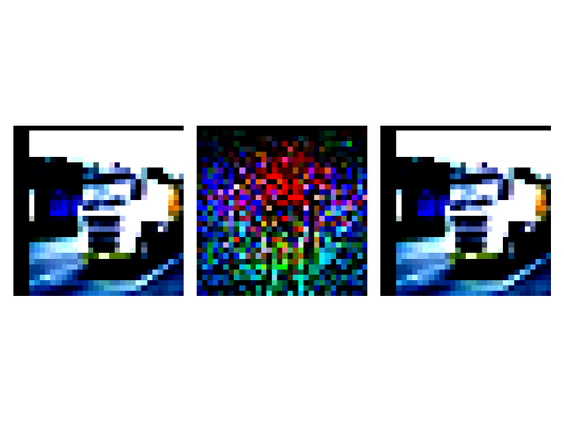
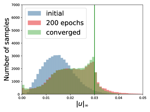
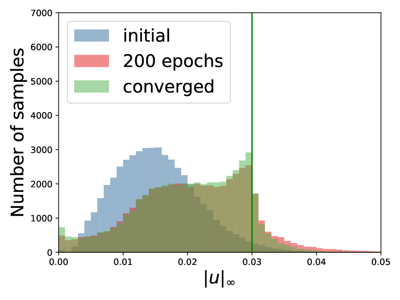
Figure 1: Results on CIFAR-10 dataset using VGG19 model: (a) usubscriptnorm𝑢\|u\|_{\infty} histogram (b) Randomly chosen image for SSDS training (left), with its corruption(center) and the corrupted image(right) (c) Evolution of usubscriptnorm𝑢\|u\|_{\infty} for the above image (d) values of v𝑣v for the above image (e) Evolution of ukuk12subscriptnormsubscript𝑢𝑘subscript𝑢𝑘12\|u_{k}-u_{k-1}\|_{2} for the above image

5 Experimental Results

In this section, we analyze the performance of SSDS algorithm empirically. We compare the effectiveness of our algorithms with the baseline SGDA algorithm and other state-of-the-art methods (e.g., PGD, TRADES, Free-m, YOPO,etc).

Experiment Setup: We present the empirical studies on the CIFAR-10, CIFAR-100 and SVHN datasets. We use VGG19 [47], ResNet50 [48], and WideResNet [49] for classification. The perturbation size is ε=0.03𝜀0.03\varepsilon=0.03, and the exponential step-size decay parameter p𝑝p is set to be 0.0010.0010.001. We initialize λ=4,ν=1.C1=C2=0.01,t=1formulae-sequenceformulae-sequence𝜆4𝜈1subscript𝐶1subscript𝐶20.01𝑡1\lambda=4,\;\nu=1.\;C_{1}=C_{2}=0.01,\;t=1 for SSDS training. The perturbation step-size is set to be η=2𝜂2\eta=2 for SGDA and SSDS training. For the purpose of consistency with other research work in this area, we use η=0.007𝜂0.007\eta=0.007 (22552255\frac{2}{255}) for crafting PGD and CW adversaries. The code is available at our GitHub repository: https://github.com/yasesf93/SSDS.

5.1 SSDS Convergence Characteristics

We begin the discussion on SSDS algorithm characteristics by observing the behavior of the perturbations involved in SSDS training. We plot the histogram of subscript\ell_{\infty}-norms of final perturbations (u) added to the training images for a few epochs during the training process (see Fig. 1(a)). This is to verify the theoretical claim that the final perturbations for the training images should converge at or below the budget. From the empirical results shown in Fig. 1(a), we make the observation that although perturbations for some images spill over the threshold value (ε=0.03𝜀0.03\varepsilon=0.03) during the course of the training process, most of the perturbations converge within the bound eventually (interestingly, a large number of the perturbations settle below the threshold). Next, we focus on a specific training sample to understand how the dynamics for different variables in the algorithm evolve during the course of the training process. We observe the dynamics of v𝑣v over the training epochs. In this experiment, v𝑣v was initialized at 111 (for all of the images in the training set), and it converges to 00 after around epoch 180180180. Similarly, as shown in Fig. 1(c), subscript\ell_{\infty}-norm of the perturbation generated for the chosen image converges to 0.0260.0260.026 which is below the specified budget. However, the actual perturbations for individual pixels still continue to evolve even after the subscript\ell_{\infty}-norm for the entire perturbation matrix settles down. To monitor the perturbations for the individual pixels, we plot 2subscript2\ell_{2} norm of the difference between the perturbations for two consecutive epochs. We see that this metric finally converges to 00 around epoch 300300300. At this point, the overall training process also converges except for small changes due to the stochastic nature of the training algorithm.

Remark 4.

Analytically and experimentally, we show that the final perturbation should remain within the budget after convergence. However, for the purpose of consistency with other algorithms we compare against, we apply the projection term to the perturbations to ensure the perturbations never exceed the budget and we call this variant SSDS-p.

Algorithm 3 Mini-batch SSDS-p algorithm
1:  Input: ε𝜀\varepsilon, lr, p𝑝p, C1subscript𝐶1C_{1}, C2subscript𝐶2C_{2}
2:  Initialization: λ0subscript𝜆0\lambda_{0}, α0subscript𝛼0\alpha_{0},w0subscript𝑤0w_{0}, t0subscript𝑡0t_{0},u0subscript𝑢0u_{0}, v0subscript𝑣0v_{0}
3:  for k{1,,K}𝑘1𝐾k\in\{1,...,K\} do
4:     distribute mini-batches as m={m0,m1,..,mn}m=\{m_{0},m_{1},..,m_{n}\}
5:     wkm0=wksuperscriptsubscript𝑤𝑘subscript𝑚0subscript𝑤𝑘w_{k}^{m_{0}}=w_{k}
6:     λkm0=λksuperscriptsubscript𝜆𝑘subscript𝑚0subscript𝜆𝑘\lambda_{k}^{m_{0}}=\lambda_{k}
7:     for mj{m0,m1,,mn}subscript𝑚𝑗subscript𝑚0subscript𝑚1subscript𝑚𝑛m_{j}\in\{m_{0},m_{1},...,m_{n}\} do
8:        wk=wkjmjL(Ij+ukj,yj,wkj)subscriptsubscript𝑤𝑘subscriptsubscript𝑤𝑘subscript𝑗subscript𝑚𝑗𝐿superscript𝐼𝑗superscriptsubscript𝑢𝑘𝑗superscript𝑦𝑗superscriptsubscript𝑤𝑘𝑗\partial_{w_{k}}=\partial_{w_{k}}\sum_{j\in m_{j}}L(I^{j}+u_{k}^{j},y^{j},w_{k}^{j})
9:        wkmj+1=wkmjlrλk(wk)superscriptsubscript𝑤𝑘subscript𝑚𝑗1superscriptsubscript𝑤𝑘subscript𝑚𝑗𝑙𝑟subscript𝜆𝑘subscriptsubscript𝑤𝑘w_{k}^{m_{j+1}}=w_{k}^{m_{j}}-lr\;\lambda_{k}(\partial_{w_{k}})
10:     end for
11:     tk+1=tk+αk(λk1)subscript𝑡𝑘1subscript𝑡𝑘subscript𝛼𝑘subscript𝜆𝑘1t_{k+1}=t_{k}+\alpha_{k}(\lambda_{k}-1)
12:     vk+1mj=vkmj+αk(ukmjε)superscriptsubscript𝑣𝑘1subscript𝑚𝑗superscriptsubscript𝑣𝑘subscript𝑚𝑗subscript𝛼𝑘subscriptnormsuperscriptsubscript𝑢𝑘subscript𝑚𝑗𝜀v_{k+1}^{m_{j}}=v_{k}^{m_{j}}+\alpha_{k}(\|u_{k}^{m_{j}}\|_{\infty}-\varepsilon)
13:     uk=ukL(Imj+ukmj,ymj,wkmj)subscriptsubscript𝑢𝑘subscriptsubscript𝑢𝑘𝐿superscript𝐼subscript𝑚𝑗superscriptsubscript𝑢𝑘subscript𝑚𝑗superscript𝑦subscript𝑚𝑗superscriptsubscript𝑤𝑘subscript𝑚𝑗\partial_{u_{k}}=\partial_{u_{k}}L(I^{m_{j}}+u_{k}^{m_{j}},y^{m_{j}},w_{k}^{m_{j}})
14:     uk+1mj=ukmj+αk(ukC1vkmjsign(ukmj))superscriptsubscript𝑢𝑘1subscript𝑚𝑗superscriptsubscript𝑢𝑘subscript𝑚𝑗subscript𝛼𝑘subscriptsubscript𝑢𝑘subscript𝐶1superscriptsubscript𝑣𝑘subscript𝑚𝑗signsuperscriptsubscript𝑢𝑘subscript𝑚𝑗u_{k+1}^{m_{j}}=u_{k}^{m_{j}}+\alpha_{k}(\partial_{u_{k}}-C_{1}\;v_{k}^{m_{j}}\operatorname*{sign}(u_{k}^{m_{j}}))
15:     for jmj𝑗subscript𝑚𝑗j\in m_{j} do
16:        Bj=(ukjε)superscript𝐵𝑗subscriptnormsuperscriptsubscript𝑢𝑘𝑗𝜀B^{j}=(\|u_{k}^{j}\|_{\infty}-\varepsilon)
17:        Uj=(L(Ij+ukj,yj,wkj)vkj)Bjsuperscript𝑈𝑗𝐿superscript𝐼𝑗superscriptsubscript𝑢𝑘𝑗superscript𝑦𝑗superscriptsubscript𝑤𝑘𝑗superscriptsubscript𝑣𝑘𝑗superscript𝐵𝑗U^{j}=\big{(}L(I^{j}+u_{k}^{j},y^{j},w_{k}^{j})-v_{k}^{j}\big{)}B^{j}
18:     end for
19:     U=jmjU(j)𝑈subscript𝑗subscript𝑚𝑗superscript𝑈𝑗U=\sum_{j\in m_{j}}U^{(j)}
20:     λk+1mj=λkmj+C2αk(Utk)superscriptsubscript𝜆𝑘1subscript𝑚𝑗superscriptsubscript𝜆𝑘subscript𝑚𝑗subscript𝐶2subscript𝛼𝑘𝑈subscript𝑡𝑘\lambda_{k+1}^{m_{j}}=\lambda_{k}^{m_{j}}+C_{2}\;\alpha_{k}\Big{(}U-t_{k}\Big{)}
21:     λk+1mjΠ(λk+1mj)superscriptsubscript𝜆𝑘1subscript𝑚𝑗Πsuperscriptsubscript𝜆𝑘1subscript𝑚𝑗\lambda_{k+1}^{m_{j}}\leftarrow\Pi(\lambda_{k+1}^{m_{j}})   (ΠΠ\Pi is the projection operator)
22:     wk=wkmnsubscript𝑤𝑘superscriptsubscript𝑤𝑘subscript𝑚𝑛w_{k}=w_{k}^{m_{n}}
23:     λk=λk+1mnsubscript𝜆𝑘superscriptsubscript𝜆𝑘1subscript𝑚𝑛\lambda_{k}=\lambda_{k+1}^{m_{n}}
24:     αk+1=αkekpsubscript𝛼𝑘1subscript𝛼𝑘superscript𝑒𝑘p\alpha_{k+1}=\alpha_{k}e^{-k\textit{p}}
25:  end for

5.2 SSDS vs SSDS-p Convergence Results

As discussed in the main paper, we can show theoretically and experimentally that although the perturbations might spill over the threshold value (ε=0.03𝜀0.03\varepsilon=0.03) for some epochs, they will converge at or below the threshold after the convergence. However, to be consistent with other research works in this area, we apply a projection term to ensure that the perturbations always remain within the budge during the training process which results in the SSDS-p which is presented in Algorithm 3.

As Fig 2 shows, by applying SSDS-p training the subscript\ell_{\infty} norm of the perturbations (usubscriptnorm𝑢\|u\|_{\infty}) always stays withing the boundary (Fig 2(b)) whereas without the projection (Fig 2(a)) the perturbations may spill over the boundary.
Refer to caption
(a)
Refer to caption
(b)
Figure 2: CIFAR-10 dataset trained using SSDS vs SSDS-p algorithm, VGG19 model architecture: (a) Histogram of usubscriptnorm𝑢\|u\|_{\infty} for SSDS (b) Histogram of usubscriptnorm𝑢\|u\|_{\infty} for SSDS-p

5.3 SSDS-p performance comparison with SGDA as defense methods

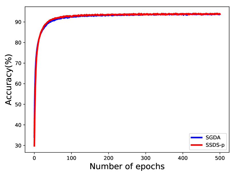
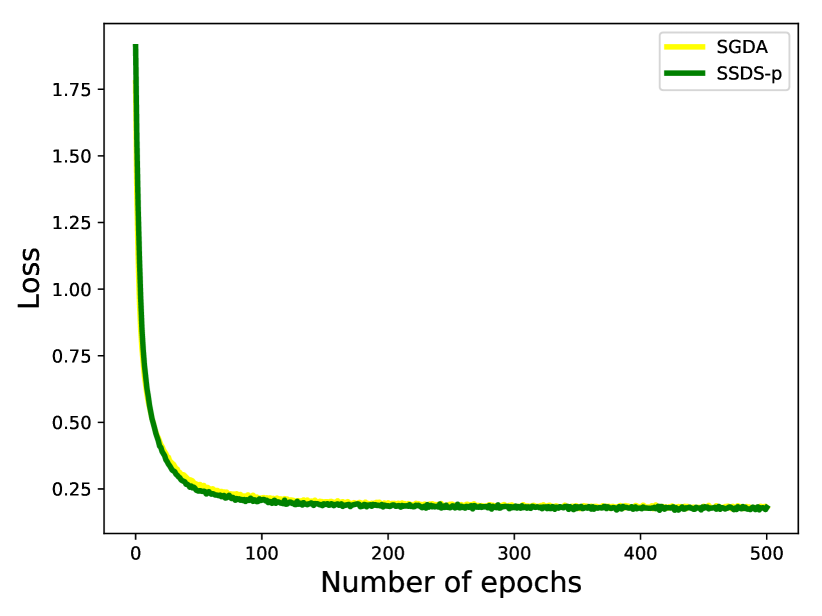
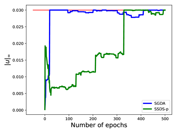
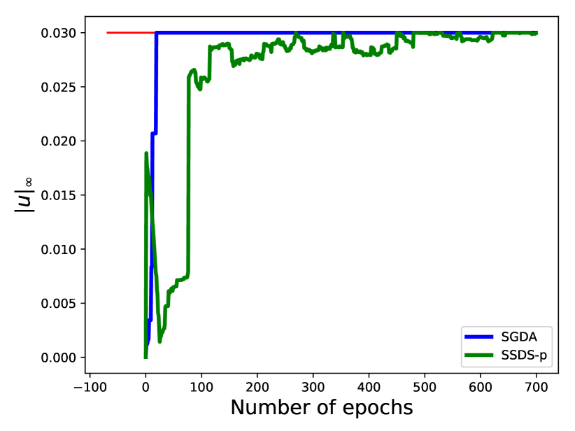
Unlike the computationally expensive techniques such as PGD training, both SGDA and SSDS-p compute the optimal perturbations/attacks cumulatively over the training epochs. Therefore, we begin this comparison between SGDA and SSDS-p algorithms by comparing the training schemes associated with each algorithm. As figures  4(a) and 4(b) show, the training scheme is very similar for SGDA and SSDS-p. However, the perturbation evolution is quite different. Fig 3 shows the subscript\ell_{\infty} norm of the perturbations added to a randomly selected images. In the case of SSDS-p training, the perturbation evolves gradually through the training epochs. On the other hand, for the SGDA method, the perturbation rapidly reaches the budget, and the method does not seem to explore the perturbations with lower magnitudes as much as SSDS-p. We note that this is a typical observation for these two algorithms. Based on the results in Table 1(b), SSDS-p algorithm performs slightly better for both clean and adversarially perturbed (across all attack algorithms considered here) input data and the marginal improvement can be attributed to better exploration of the perturbation space by the SSDS-p algorithm.

Table 1: SGDA and SSDS-p defense model (WideResNet) performance comparison under white-box attacks
Attack Accuracy
Clean 81.97%
FGSM 80.4%
PGD 44.32%
SGDA 48.58%
SSDS-p 51.64%
(a) SGDA training
Attack Accuracy
Clean 82.91 %
FGSM 81.21 %
PGD 45.89%
SGDA 49.18 %
SSDS-p 53.53 %
(b) SSDS-p training

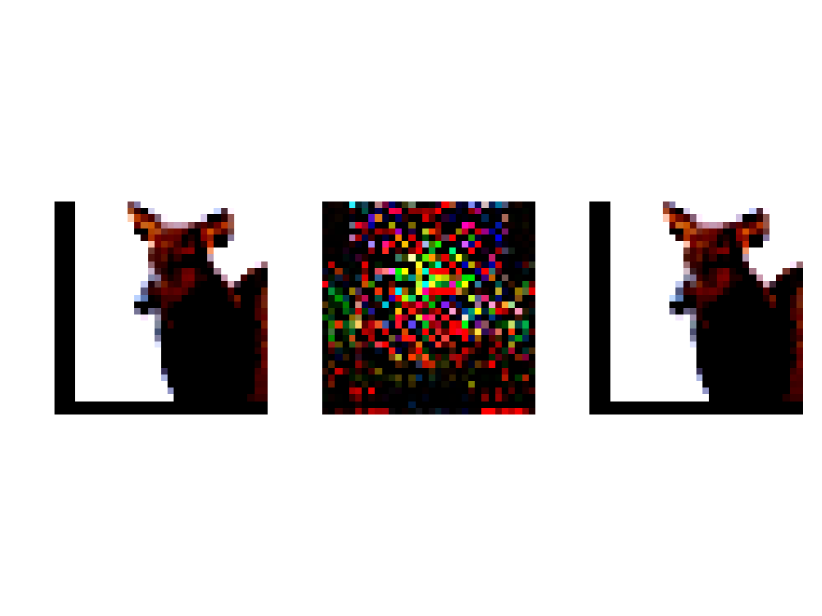
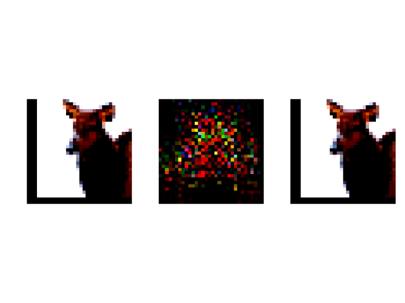
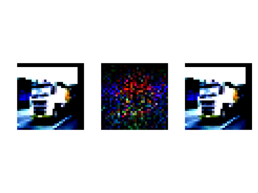
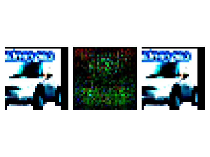
We then visualize the attack on randomly selected images. As Fig 5 suggests, the two algorithms seem to generate similar attacks although the SSDS-p attacks (Fig 5(b)) looks more gradient based. As the Lagrangian multiplier corresponding to generating the attacks (v𝑣v) controls the gradients in each epoch, the gradients play a more significant part in generation the attacks.
Refer to caption
(a)
Refer to caption
(b)
Figure 3: Evolution of perturbation/attack on two randomly selected images under SGDA and SSDS-p training
Refer to caption
(a)
Refer to caption
(b)
Figure 4: SGDA vs SSDS-p comparison on CIFAR-10 dataset, WideResNet model architecture: (a) Accuracy (b) Loss value
Refer to caption
Refer to caption
Refer to caption
Refer to caption
Refer to caption
(a)
Refer to caption
(b)
Figure 5: SGDA vs SSDS-p comparison on CIFAR-10 dataset, WideResNet model architecture: (a) Randomly chosen image for SGDA training (left), with its corruption(center) and the corrupted image (right) (b) Randomly chosen image for SSDS-p training (left), with its corruption (center) and the corrupted image(right)

5.4 SSDS-p and SGDA attacks

Algorithm 4 SGDA attack algorithm
1:  Input: ε𝜀\varepsilon, p𝑝p, wsuperscript𝑤w^{\star}
2:  Initialization:u0subscript𝑢0u_{0}, α0subscript𝛼0\alpha_{0}
3:  for k{1,,K}𝑘1𝐾k\in\{1,...,K\} do
4:     uk+1(mj)=uk(mj)+αk(ukL(I(mj)+uk(mj),y(mj),w)u_{k+1}^{(m_{j})}=u_{k}^{(m_{j})}+\alpha_{k}(\partial_{u_{k}}L(I^{(m_{j})}+u_{k}^{(m_{j})},y^{(m_{j})},w^{\star})
5:     αk+1=αkekpsubscript𝛼𝑘1subscript𝛼𝑘superscript𝑒𝑘p\alpha_{k+1}=\alpha_{k}e^{-k\textit{p}}
6:  end for

Throughout the paper, we discussed the performance of SSDS-p and SGDA algorithms as defense method against adversarial perturbations. However, SSDS-p and SGDA attacks can be generated through an iterative process by freezing the model (wsuperscript𝑤w^{\star}s) and following the same algorithm for updating u𝑢us. Note that, for generating SSDS-p attacks λ𝜆\lambda is not getting updated too as it corresponds to the model parameters, whereas v𝑣vs are being updated in the same fashion in SSDS-p training. Algorithms 4, 5 are the corresponding attack algorithms for SGDA and SSDS-p methods.

Algorithm 5 SSDS attack algorithm
1:  Input: ε𝜀\varepsilon, p𝑝p, C1subscript𝐶1C_{1}, wsuperscript𝑤w^{\star}
2:  Initialization:u0subscript𝑢0u_{0}, v0subscript𝑣0v_{0}, α0subscript𝛼0\alpha_{0}
3:  for k{1,,K}𝑘1𝐾k\in\{1,...,K\} do
4:     vk+1(mj)=vk(mj)+αk(uk(mj)ε)superscriptsubscript𝑣𝑘1subscript𝑚𝑗superscriptsubscript𝑣𝑘subscript𝑚𝑗subscript𝛼𝑘subscriptnormsuperscriptsubscript𝑢𝑘subscript𝑚𝑗𝜀v_{k+1}^{(m_{j})}=v_{k}^{(m_{j})}+\alpha_{k}(\|u_{k}^{(m_{j})}\|_{\infty}-\varepsilon)
5:     uk+1(mj)=uk(mj)+αk(ukL(I(mj)+uk(mj),y(mj),w)C1vk(mj)sign(uk(mj)))superscriptsubscript𝑢𝑘1subscript𝑚𝑗superscriptsubscript𝑢𝑘subscript𝑚𝑗subscript𝛼𝑘subscriptsubscript𝑢𝑘𝐿superscript𝐼subscript𝑚𝑗superscriptsubscript𝑢𝑘subscript𝑚𝑗superscript𝑦subscript𝑚𝑗superscript𝑤subscript𝐶1superscriptsubscript𝑣𝑘subscript𝑚𝑗signsuperscriptsubscript𝑢𝑘subscript𝑚𝑗u_{k+1}^{(m_{j})}=u_{k}^{(m_{j})}+\alpha_{k}(\partial_{u_{k}}L(I^{(m_{j})}+u_{k}^{(m_{j})},y^{(m_{j})},w^{\star})-C_{1}\;v_{k}^{(m_{j})}\operatorname*{sign}(u_{k}^{(m_{j})}))
6:     αk+1=αkekpsubscript𝛼𝑘1subscript𝛼𝑘superscript𝑒𝑘p\alpha_{k+1}=\alpha_{k}e^{-k\textit{p}}
7:  end for

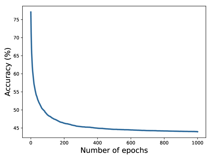
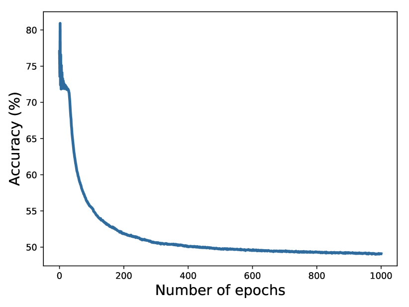
Fig. 6 shows the performance of a well trained (SGDA) model on SSDS-p and SGDA attacks. The plots show that the model performs well and the testing accuracy is high in the beginning when the optimal attack is still not found, but as the final perturbation is crafted, the accuracy stays fixed and the test accuracies under SGDA and SSDS-p optimal attacks are achieved.
Refer to caption
(a) SGDA test accuracy
Refer to caption
(b) SSDS-p test accuracy
Figure 6: Testing accuracy plots for SGDA robust model under (a) SGDA (b) SSDS-p attacks (dataset: CIFAR10, ε=0.03𝜀0.03\varepsilon=0.03, model architecture: VGG19)

5.5 SSDS-p performance evaluation and comparison

In this section, we present a detailed performance evaluation of the proposed SSDS-p algorithm under both white-box and black-box attacks. We compare the performance of SSDS-p with the state-of-the-art robust learning algorithms.

Table 2: Performance comparison of several robust learning methods under white-box attacks using WideResNet on CIFAR-10 dataset
Defence model Clean FGSM PGD-20
Natural 94.82% 35.23% 5.93%
FeatureScatter [39] 90.00% 78.40% 70.50%
Free-8 [17] 85.96% 53.57% 46.82%
PGD-7 [14] 85.70% 54.90% 44.90%
FGSM+DAWNBench [25] 83.12% 59.17% 45.18%
YOPO [22] 86.70% 55.23% 47.98%
TRADES [16] 84.92% 61.06% 56.61%
SGDA 81.97% 80.40% 44.32%
SSDS-p 82.91% 81.21% 45.89%

CIFAR-10 dataset Under white-box attacks:

We present the performance of SSDS-p under white-box attacks (with FGSM and PGD attack models) in Table 2 along with other state-of-the-art defense models. We also provide SGDA performance in the table as a baseline for our proposed approach. Based on the results presented, SSDS-p performs the best under FGSM attack, which is a computationally inexpensive attack. Under computationally expensive attacks using the PGD-20 algorithm (i.e., PGD with 20 step iteration), SSDS-p performance is comparable with the PGD-7, Free-8, FGSM+DAWNBench, and YOPO defence algorithms. However, as Table 11 suggests, while FeatureScatter, PGD, YOPO and TRADES training algorithms are significantly more computationally complex compared to SSDS-p, other algorithms (Free-8, FGSM+DAWNBench) have comparable accuracy and running time with SSDS-p. Comparing the performance of different algorithms in Table 2, we can see that only TRADES and FeatureScatter algorithm perform significantly better than all other methods under the PGD-20 attack. However, the methodology for generating the perturbations and using them eventually for training their robust model is different in FeatureScatter. In FeatureScatter [39], adversarial examples are generated for training through feature scattering in the latent space, which is unsupervised in nature and computationally expensive. Similarly, while SSDS-p along with other methods listed in the table use cross entropy loss function, TRADES [16] differs in terms of the objective function and is still quite expensive computationally, similar to PGD training.

CIFAR-10 dataset Under black-box attacks:

We evaluate our proposed SSDS-p method under black-box attacks as well as compare head-to-head performance against PGD and TRADES approaches. As we wanted to use pre-trained PGD and TRADES models available online for this study, we had to use only ResNet50 architecture while comparing with the PGD-trained model and WideResNet architecture for comparison with the TRADES model. For the comparison with PGD training, we use the SSDS-p ResNet50 model for defending against 202020 step PGD attacks generated using a naturally trained model as well as using the pre-trained PGD model [50] available online as source models. We also evaluate the performance of the PGD above model under 20-step PGD attacks generated using the naturally trained and the SSDS-p models as source models. Results presented in Table 3 show that SSDS-p performs significantly better than the PGD model under black-box attacks. In order to compare with TRADES models, we use the pre-trained WideResNet TRADES model, which is available online. Based on similar experiments, it is evident that SSDS-p also performs better than the TRADES model under black-box attacks (as shown in Table 4).

Table 3: Black box performance: 20 step PGD attacks crafted by naturally trained model, SSDS-p trained model and PGD trained model [50] using ResNet50 architecture on CIFAR-10 dataset
Target Source Attack Accuracy
PGD-7 naturally-trained PGD-20 75.15%
SSDS-p naturally-trained PGD-20 78.59%
PGD-7 SSDS-p PGD-20 71.62%
SSDS-p PGD PGD-20 78.53%
Table 4: Black box performance: 20 step PGD attacks crafted by naturally trained model, SSDS-p trained model and TRADES trained model [16] using WideResNet architecture on CIFAR-10 dataset
Target Source Attack Accuracy
TRADES naturally-trained PGD-20 66.97%
SSDS-p naturally-trained PGD-20 74.37%
TRADES SSDS-p PGD-20 66.82%
SSDS-p TRADES PGD-20 80.63%

CIFAR-100 dataset under white-box attacks:

We present the performance of SGDA, and SSDS-p under white-box attacks in Table 5 and compare them with state-of-the-art methods. Similar to CIFAR-10 results, the performance of SSDS-p algorithm is better that Free-8 and PGD-7 robust models under FGSM attacks, and comparable with PGD-7 under PGD-20 attack. FeatureScatter still achieves the highest accuracy among all the methods but as we mentioned earlier it uses feature scattering techniques in the latent space to generate adversaries which makes it computationally expensive.

Table 5: Performance comparison of several robust learning methods under white-box attacks using WideResNet on CIFAR-100 dataset
Defence model Clean FGSM PGD-20
Natural 74.00% 10.75% 0.00%
FeatureScatter [39] 73.90% 61.00% 47.20%
Free-8 [17] 62.13% 29.14% 25.88%
PGD-7 [14] 59.90% 28.50% 22.60%
SGDA 49.11% 48.01% 16.33%
SSDS-p 50.85% 49.49% 19.01%

CIFAR-100 dataset under black-box attacks:

We evaluate our proposed SSDS-p method under black-box attacks and compare the performance with SGDA. We use the SSDS-p WideResNet model for defending against 202020 step PGD attacks generated using a naturally trained model as well as using the pre-trained SGDA model as source models. We also evaluate the performance of the above SGDA model under 20-step PGD attacks generated using the naturally trained and the SSDS-p models as source models. Results presented in Table 6 show that SSDS-p performs slightly better than the SGDA model under black-box attacks similar to the performance under white-box attacks.

Table 6: Black box performance: 20 step PGD attacks crafted by naturally trained model, SSDS-p trained model and SGDA trained model using WideResNet model architecture on CIFAR-100 dataset
Target Source Attack Accuracy
SGDA naturally-trained PGD-20 42.50%
SSDS-p naturally-trained PGD-20 44.08%
SGDA SSDS-p PGD-20 41.12%
SSDS-p SGDA PGD-20 42.70%

SVHN dataset under white-box attacks:

We present the performance of SGDA, and SSDS-p under white-box attacks in Table 7 and compare them with stat-of-the-art methods. Results show that the performance of our SSDS-p algorithm is comparable to FeatureScatter under most of the attack schemes. We can provide more robust model compared to PGD-7 as well in significantly less time (refer to Table 11).

Table 7: Performance comparison of several robust learning methods under white-box attacks using ResNet50 on SVHN dataset:
Defence model Clean FGSM PGD-20 PGD-100 CW-20 CW-100
Natural 97.20% 53.00% 0.3% 0.1% 0.3% 0.1%
PGD-7 [14] 93.9% 68.4% 47.9% 46.0% 48.7% 47.3%
FeatureScatter [39] 96.2% 83.5% 62.9% 52.0% 61.3% 50.8%
SGDA 93.97% 69.82% 52.52% 52.34% 52.42% 52.35%
SSDS-p 94.32 % 73.53% 61.39% 61.33% 61.07% 60.94

SSDS-p with different model architectures:

To further analyse the algorithm, we have evaluated the performance of our model on other model architectures (e.g., ResNet50 and VGG19). Table 8 summarizes the performance of SSDS-p using ResNet50 model architecture along with other training methods on CIFAR-10 and CIFAR-100 datasets. Results align with Table 2 where SSDS-p performs the best under FGSM attack and the the model is comparable to PGD-7 model under PGD-20 attacks. Similarly, results on CIFAR-100 dataset shows that SSDS-p performs the best compared to SGDA and naturally trained models using ResNet model architecture.

Additionally, as the model architectures play a significant role specially when the input data is large, we run SSDS-p on different model architectures to analyse the dependency of SSDS-p on the model capacity, gradients, etc. Based on Table 9(c), we see that the model capacity and complexity definitely helps both natural and robust accuracy, although the effect is not as significant as its effect on PGD robust models reported by Madry et al. [14].

Table 8: Performance comparison of several training methods under white-box attacks using ResNet50 on CIFAR-10 dataset
Dataset Defence model Clean FGSM PGD-20
CIFAR-10 Natural 92.70% 27.50% 0.82%
CIFAR-10 PGD-7 79.4% 51.7% 43.7%
CIFAR-10 SGDA 78.04% 76.42% 40.70%
CIFAR-10 SSDS-p 80.1% 79.32% 42.11 %
CIFAR-100 Natural 47.96% 43.66% 13.01%
CIFAR-100 SGDA 47.07% 46.18% 18.16%
CIFAR-100 SSDS-p 49.77% 49.22% 19.69 %
Table 9: SSDS-p defense with different model architectures under white-box attacks
Attack Accuracy
Clean 77.13%
FGSM 75.92%
PGD 42.32%
SGDA 43.49%
SSDS-p 47.56%
(a) VGG 19
Attack Accuracy
Clean 80.10 %
FGSM 79.32 %
PGD 42.11%
SGDA 44.58 %
SSDS-p 50.09 %
(b) ResNet50
Attack Accuracy
Clean 82.91 %
FGSM 81.21 %
PGD 45.89%
SGDA 49.18 %
SSDS-p 53.53 %
(c) WideResNet

Attacks with more number of steps

To further evaluate our algorithm, We present the performance of SGDA, and SSDS-p under PGD and CW white-box attacks with various steps. The results are summarized in Tables 10 for CIFAR-10 and CIFAR-100 datasets. Similar to other robust models, SSDS-p can preserve the performance when the number of steps increase (the generated attacks become more powerful).

Table 10: Performance comparison of several robust learning methods under white-box attacks using WideResNet
Dataset Defence model PGD-10 PGD-40 PGD-100 CW-20 CW-100
CIFAR-10 Natural 7.83% 4.18% 0% 4.73% 0.32%
CIFAR-10 FeatureScatter [39] 70.90% 70.3% 68.60% 62.40% 60.6%
CIFAR-10 PGD-7 [14] 45.10% 44.80% 44.80% 45.70% 45.40%
CIFAR-10 SGDA 45.74% 44.05% 44.03% 44.82% 44.66%
CIFAR-10 SSDS-p 47.35% 45.61% 46.44% 46.62% 46.40%
CIFAR-100 Natural 12.83% 9.61% 6.42% 12.13% 7.21%
CIFAR-100 SGDA 18.85% 16.09% 15.76% 16.52% 16.37%
CIFAR-100 SSDS-p 19.23% 16.15% 16.10% 16.78% 16.70%

5.6 Computational time comparison

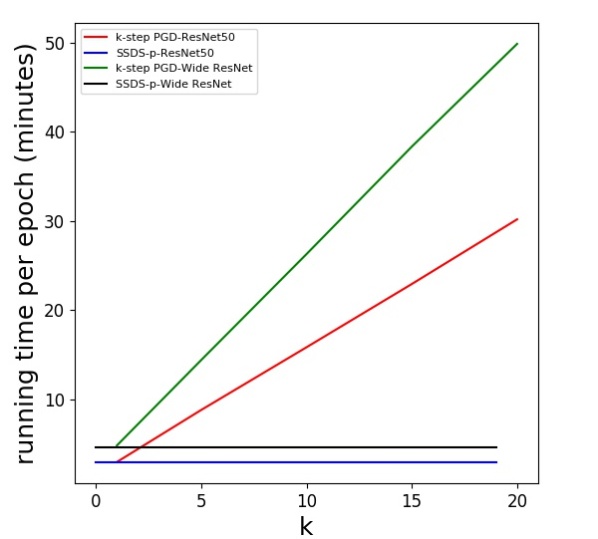
One of the key advantages of our proposed algorithm is the significantly lower computational overhead compared to the standard techniques for training robust models. To demonstrate this, we compare computation times with experiments run on one node of a GPU cluster with Intel Xeon Processor with 32 cores, 128GB RAM and with a Titan X (Pascal architecture) GPU having 12GB of GPU RAM. Fig. 7 shows that although PGD-7 and SSDS-p achieve comparable robust classification accuracy for CIFAR-10 dataset, the training time per epoch for 7 step PGD-training algorithm is approximately 444 times greater than that of the SSDS-p training algorithm. On the other hand, SSDS-p training takes around the same time as a 111 step PGD training (or FGSM-based adversarial training). Table 11 summarizes the running time corresponding to other state-of-the-art algorithms. SSDS-p (similar to Free-8 and FGSM+DAWNBench) can achieve comparable accuracy with PGD in significantly less time. FeatureScatter which is the most accurate compared to other algorithms is computationally very expensive. In summary, our approach is a computationally efficient framework for robust learning compared to most of the state-of-the-art techniques.
Refer to caption
Figure 7: Training time per epoch for PGD vs. SSDS-p
Table 11: Running time comparison of several robust learning methods using WideResNet and Cifar-10 dataset:
Defence model Time (seconds per epoch)
Free-8 [17] 289
FeatureScatter [39] 3132
FGSM+DAWNBench [25] 296
YOPO [22] 790
FGSM [6] 295
PGD-7 [14] 1269
PGD-20 [14] 3011
TRADES [16] 1006
SSDS-p 291

6 Conclusion

In this paper, we propose a new stochastic saddle-point dynamical systems approach to solve the robust learning problem. Under certain restrictive assumptions, we present a detailed convergence analysis of our algorithm. Our proposed algorithm involves a Lagrangian formulation to solve the robust optimization problem, where we introduce two Lagrangian multipliers for both model parameters and uncertainties. The multiplier for the uncertainties allows us to handle more complex uncertainty constraints where the uncertainties are assumed to belong to more general convex sets, for example ellipsoids or intersections of ellipsoids. In the absence of a multiplier to impose these constraints on the uncertainty set, one will have to resort to solving an optimization problem within another optimization problem, thereby making the rigorous convergence proof of such algorithm quite difficult. Our approach is useful even for the case when the uncertainty has a simple constraint. For example, an subscript\ell_{\infty} norm bounded uncertainty can be imposed by simple projection. However, obtaining rigorous convergence proof of an algorithm consisting of a multiplier to impose the parameter constraints and simple projection to impose the uncertainty constraints is difficult and does not exist. Similar justification applies to using Lagrangian multipliers for model parameters, especially since the constraints on the model parameters are more complicated than simple box constraints. In addition to these advantages, we also observe performance improvement over the baseline SGDA algorithm that does not use the Lagrangian multipliers. Empirically, we show that the proposed scheme is a computationally inexpensive method that maintains a high level of performance for clean and corrupted input data, both for white-box and black-box attacks. We believe that this can be attributed to the adversarial training in SSDS also acts as a form of regularization. We can explain it based on the equivalence between the robust optimization problem and many regularization problems [43]. Finally, we note that this is an early attempt to adopting a dynamical systems approach to robust learning. Future research will focus on relaxing some of the restrictive assumptions in the analysis for the loss function and uncertainties. Similarly, we will focus on developing the SSDS algorithm further by modifying the cost functions to better handle the highly non-convex nature of deep network loss functions, leading to performance improvement.

References

  • Sitawarin et al. [2018] Chawin Sitawarin, Arjun Nitin Bhagoji, Arsalan Mosenia, Mung Chiang, and Prateek Mittal. Darts: Deceiving autonomous cars with toxic signs. arXiv preprint arXiv:1802.06430, 2018.
  • Biggio et al. [2013] Battista Biggio, Igino Corona, Davide Maiorca, Blaine Nelson, Nedim Šrndić, Pavel Laskov, Giorgio Giacinto, and Fabio Roli. Evasion attacks against machine learning at test time. In Joint European conference on machine learning and knowledge discovery in databases, pages 387–402. Springer, 2013.
  • Haghighat et al. [2020] Arya Ketabchi Haghighat, Varsha Ravichandra-Mouli, Pranamesh Chakraborty, Yasaman Esfandiari, Saeed Arabi, and Anuj Sharma. Applications of deep learning in intelligent transportation systems. Journal of Big Data Analytics in Transportation, 2(2):115–145, 2020.
  • Hosseini and Smadi [2021] Seyed Amirhossein Hosseini and Omar Smadi. How prediction accuracy can affect the decision-making process in pavement management system. Infrastructures, 6(2):28, 2021.
  • Carlini and Wagner [2017] Nicholas Carlini and David Wagner. Towards evaluating the robustness of neural networks. In 2017 IEEE Symposium on Security and Privacy (SP), pages 39–57. IEEE, 2017.
  • Goodfellow et al. [2014] Ian J Goodfellow, Jonathon Shlens, and Christian Szegedy. Explaining and harnessing adversarial examples. arXiv preprint arXiv:1412.6572, 2014.
  • Kurakin et al. [2016] Alexey Kurakin, Ian Goodfellow, and Samy Bengio. Adversarial examples in the physical world. arXiv preprint arXiv:1607.02533, 2016.
  • Szegedy et al. [2013] Christian Szegedy, Wojciech Zaremba, Ilya Sutskever, Joan Bruna, Dumitru Erhan, Ian Goodfellow, and Rob Fergus. Intriguing properties of neural networks. arXiv preprint arXiv:1312.6199, 2013.
  • Moosavi-Dezfooli et al. [2016] Seyed-Mohsen Moosavi-Dezfooli, Alhussein Fawzi, and Pascal Frossard. Deepfool: a simple and accurate method to fool deep neural networks. In Proceedings of the IEEE conference on computer vision and pattern recognition, pages 2574–2582, 2016.
  • Yao et al. [2019] Zhewei Yao, Amir Gholami, Peng Xu, Kurt Keutzer, and Michael W Mahoney. Trust region based adversarial attack on neural networks. In Proceedings of the IEEE Conference on Computer Vision and Pattern Recognition, pages 11350–11359, 2019.
  • Papernot et al. [2017] Nicolas Papernot, Patrick McDaniel, Ian Goodfellow, Somesh Jha, Z Berkay Celik, and Ananthram Swami. Practical black-box attacks against machine learning. In Proceedings of the 2017 ACM on Asia conference on computer and communications security, pages 506–519. ACM, 2017.
  • Bertsimas et al. [2011] Dimitris Bertsimas, David B Brown, and Constantine Caramanis. Theory and applications of robust optimization. SIAM review, 53(3):464–501, 2011.
  • Ben-Tal et al. [2009] Aharon Ben-Tal, Laurent El Ghaoui, and Arkadi Nemirovski. Robust optimization, volume 28. Princeton University Press, 2009.
  • Madry et al. [2017] Aleksander Madry, Aleksandar Makelov, Ludwig Schmidt, Dimitris Tsipras, and Adrian Vladu. Towards deep learning models resistant to adversarial attacks. arXiv preprint arXiv:1706.06083, 2017.
  • Danskin [1966] John M Danskin. The theory of max-min, with applications. SIAM Journal on Applied Mathematics, 14(4):641–664, 1966.
  • Zhang et al. [2019a] Hongyang Zhang, Yaodong Yu, Jiantao Jiao, Eric P. Xing, Laurent El Ghaoui, and Michael I. Jordan. Theoretically principled trade-off between robustness and accuracy. CoRR, abs/1901.08573, 2019a. URL http://arxiv.org/abs/1901.08573.
  • Shafahi et al. [2019] Ali Shafahi, Mahyar Najibi, Amin Ghiasi, Zheng Xu, John Dickerson, Christoph Studer, Larry S. Davis, Gavin Taylor, and Tom Goldstein. Adversarial training for free!, 2019.
  • Fawzi et al. [2016] Alhussein Fawzi, Seyed-Mohsen Moosavi-Dezfooli, and Pascal Frossard. Robustness of classifiers: from adversarial to random noise. In Advances in Neural Information Processing Systems, pages 1632–1640, 2016.
  • Shaham et al. [2018] Uri Shaham, Yutaro Yamada, and Sahand Negahban. Understanding adversarial training: Increasing local stability of supervised models through robust optimization. Neurocomputing, 307:195–204, 2018.
  • Lin et al. [2019] Tianyi Lin, Chi Jin, and Michael I Jordan. On gradient descent ascent for nonconvex-concave minimax problems. arXiv preprint arXiv:1906.00331, 2019.
  • Sinha et al. [2017] Aman Sinha, Hongseok Namkoong, Riccardo Volpi, and John Duchi. Certifying some distributional robustness with principled adversarial training. arXiv preprint arXiv:1710.10571, 2017.
  • Zhang et al. [2019b] Dinghuai Zhang, Tianyuan Zhang, Yiping Lu, Zhanxing Zhu, and Bin Dong. You only propagate once: Accelerating adversarial training via maximal principle. In Advances in Neural Information Processing Systems, pages 227–238, 2019b.
  • Wong et al. [2018] Eric Wong, Frank Schmidt, Jan Hendrik Metzen, and J Zico Kolter. Scaling provable adversarial defenses. In Advances in Neural Information Processing Systems, pages 8400–8409, 2018.
  • Krizhevsky et al. [2014] Alex Krizhevsky, Vinod Nair, and Geoffrey Hinton. The cifar-10 dataset. online: http://www. cs. toronto. edu/kriz/cifar. html, 55, 2014.
  • Wong et al. [2020] Eric Wong, Leslie Rice, and J Zico Kolter. Fast is better than free: Revisiting adversarial training. arXiv preprint arXiv:2001.03994, 2020.
  • Coleman et al. [2017] Cody Coleman, Deepak Narayanan, Daniel Kang, Tian Zhao, Jian Zhang, Luigi Nardi, Peter Bailis, Kunle Olukotun, Chris Ré, and Matei Zaharia. Dawnbench: An end-to-end deep learning benchmark and competition. Training, 100(101):102, 2017.
  • Khalid et al. [2018] Faiq Khalid, Muhammad Abdullah Hanif, Semeen Rehman, and Muhammad Shafique. Security for machine learning-based systems: Attacks and challenges during training and inference. In 2018 International Conference on Frontiers of Information Technology (FIT), pages 327–332. IEEE, 2018.
  • Barreno et al. [2010] Marco Barreno, Blaine Nelson, Anthony D Joseph, and J Doug Tygar. The security of machine learning. Machine Learning, 81(2):121–148, 2010.
  • Lin et al. [2017] Yen-Chen Lin, Zhang-Wei Hong, Yuan-Hong Liao, Meng-Li Shih, Ming-Yu Liu, and Min Sun. Tactics of adversarial attack on deep reinforcement learning agents. In Proceedings of the Twenty-Sixth International Joint Conference on Artificial Intelligence, IJCAI-17, pages 3756–3762, 2017. doi: 10.24963/ijcai.2017/525. URL https://doi.org/10.24963/ijcai.2017/525.
  • Havens et al. [2018] Aaron Havens, Zhanhong Jiang, and Soumik Sarkar. Online robust policy learning in the presence of unknown adversaries. In Advances in Neural Information Processing Systems, pages 9916–9926, 2018.
  • Tan et al. [2020a] Kai Liang Tan, Yasaman Esfandiari, Xian Yeow Lee, Soumik Sarkar, et al. Robustifying reinforcement learning agents via action space adversarial training. In 2020 American control conference (ACC), pages 3959–3964. IEEE, 2020a.
  • Lee et al. [2020] Xian Yeow Lee, Yasaman Esfandiari, Kai Liang Tan, and Soumik Sarkar. Query-based targeted action-space adversarial policies on deep reinforcement learning agents. arXiv preprint arXiv:2011.07114, 2020.
  • Tan et al. [2020b] Kai Liang Tan, Anuj Sharma, and Soumik Sarkar. Robust deep reinforcement learning for traffic signal control. Journal of Big Data Analytics in Transportation, pages 1–12, 2020b.
  • Santurkar et al. [2019] Shibani Santurkar, Dimitris Tsipras, Brandon Tran, Andrew Ilyas, Logan Engstrom, and Aleksander Madry. Computer vision with a single (robust) classifier. CoRR, abs/1906.09453, 2019. URL http://arxiv.org/abs/1906.09453.
  • Joshi et al. [2019] Ameya Joshi, Amitangshu Mukherjee, Soumik Sarkar, and Chinmay Hegde. Semantic adversarial attacks: Parametric transformations that fool deep classifiers. In Proceedings of the IEEE/CVF International Conference on Computer Vision, pages 4773–4783, 2019.
  • Gu and Rigazio [2014] Shixiang Gu and Luca Rigazio. Towards deep neural network architectures robust to adversarial examples. arXiv preprint arXiv:1412.5068, 2014.
  • Bastani et al. [2016] Osbert Bastani, Yani Ioannou, Leonidas Lampropoulos, Dimitrios Vytiniotis, Aditya Nori, and Antonio Criminisi. Measuring neural net robustness with constraints. In D. D. Lee, M. Sugiyama, U. V. Luxburg, I. Guyon, and R. Garnett, editors, Advances in Neural Information Processing Systems 29, pages 2613–2621. Curran Associates, Inc., 2016. URL http://papers.nips.cc/paper/6339-measuring-neural-net-robustness-with-constraints.pdf.
  • Tramèr et al. [2017] Florian Tramèr, Alexey Kurakin, Nicolas Papernot, Ian Goodfellow, Dan Boneh, and Patrick McDaniel. Ensemble Adversarial Training: Attacks and Defenses. arXiv e-prints, art. arXiv:1705.07204, May 2017.
  • Zhang and Wang [2019] Haichao Zhang and Jianyu Wang. Defense against adversarial attacks using feature scattering-based adversarial training. In Advances in Neural Information Processing Systems, pages 1831–1841, 2019.
  • Papernot et al. [2016] Nicolas Papernot, Patrick McDaniel, Xi Wu, Somesh Jha, and Ananthram Swami. Distillation as a defense to adversarial perturbations against deep neural networks. In 2016 IEEE Symposium on Security and Privacy (SP), pages 582–597. IEEE, 2016.
  • Athalye et al. [2018] Anish Athalye, Nicholas Carlini, and David Wagner. Obfuscated gradients give a false sense of security: Circumventing defenses to adversarial examples. arXiv preprint arXiv:1802.00420, 2018.
  • Chen et al. [2017] Robert S. Chen, Brendan Lucier, Yaron Singer, and Vasilis Syrgkanis. Robust optimization for non-convex objectives. In NIPS, 2017.
  • Sra et al. [2011] S. Sra, S. Nowozin, and S. J. Wright. Optimization for Machine Learning. MIT Press, 2011.
  • Xu et al. [2009] H. Xu, C. Caramanis, and Sh. Mannor. Robust regression and lasso. In Advances in Neural Information Processing Systems, pages 1801–1808, 2009.
  • Ebrahimi et al. [2019] Keivan Ebrahimi, Nicola Elia, and Umesh Vaidya. A continuous time dynamical system approach for solving robust optimization. In European Control Conference, Naples, Italy, 2019.
  • Boyd and Vandenberghe [2004] S. Boyd and L. Vandenberghe. Convex Optimization. New York: Cambridge Univ. Press, 2004.
  • Simonyan and Zisserman [2014] Karen Simonyan and Andrew Zisserman. Very deep convolutional networks for large-scale image recognition. arXiv preprint arXiv:1409.1556, 2014.
  • He et al. [2015] Kaiming He, Xiangyu Zhang, Shaoqing Ren, and Jian Sun. Deep residual learning for image recognition, 2015.
  • Zagoruyko and Komodakis [2016] Sergey Zagoruyko and Nikos Komodakis. Wide residual networks. arXiv preprint arXiv:1605.07146, 2016.
  • Engstrom et al. [2019] Logan Engstrom, Andrew Ilyas, Shibani Santurkar, and Dimitris Tsipras. Robustness (python library), 2019. URL https://github.com/MadryLab/robustness.

7 Supplementary Material

Additional theoretical analysis, convergence proofs and experimental results are discussed here; also more information about the material in the main body of the paper is presented.

7.1 Additional Theorems and Derivations

As we discussed in the main paper, the robust learning problem is:

𝒪:=assign𝒪absent\displaystyle{\cal RO}:= minw𝔼(I,y)𝒟[maxu𝒰L(I+u,y,w)]subscript𝑤subscript𝔼similar-to𝐼𝑦𝒟delimited-[]𝑢𝒰𝐿𝐼𝑢𝑦𝑤\displaystyle\min_{w}\;\mathbb{E}_{(I,y)\sim{\cal D}}\;\Big{[}\underset{u\in{\cal U}}{\max}\;\;L(I+u,y,w)\Big{]}\; (14)

and the total Lagrangian can be written as:

(x,λ,u,v):=assign𝑥𝜆𝑢𝑣absent\displaystyle{\cal L}(x,\lambda,u,v):= t+λ(i=1N(L(Ii+ui,yi,w)\displaystyle\;t+\lambda\;\Big{(}\textstyle\sum_{i=1}^{N}\big{(}L(I^{i}+u^{i},y^{i},w)
vihi(ui))t)\displaystyle\;-v^{i}\;h^{i}(u^{i})\big{)}-t\Big{)}\; (15)

Then we propose the following update rules for the parameters:

xk+1=xkαk(xf(xk)+λkxg(xk,uk,ξk)),subscript𝑥𝑘1subscript𝑥𝑘subscript𝛼𝑘subscript𝑥𝑓subscript𝑥𝑘subscript𝜆𝑘subscript𝑥𝑔subscript𝑥𝑘subscript𝑢𝑘subscript𝜉𝑘\displaystyle x_{k+1}=x_{k}-\alpha_{k}(\partial_{x}f(x_{k})+\lambda_{k}\partial_{x}g(x_{k},u_{k},\xi_{k}))\;, (16)
λk+1=[λk+αk(g(xk,uk,ξk)i=1Nvkihi(uki))]+,subscript𝜆𝑘1subscriptdelimited-[]subscript𝜆𝑘subscript𝛼𝑘𝑔subscript𝑥𝑘subscript𝑢𝑘subscript𝜉𝑘superscriptsubscript𝑖1𝑁superscriptsubscript𝑣𝑘𝑖superscript𝑖subscriptsuperscript𝑢𝑖𝑘\displaystyle\lambda_{k+1}=\big{[}\lambda_{k}+\alpha_{k}\big{(}g(x_{k},u_{k},\xi_{k})-\textstyle\sum_{i=1}^{N}v_{k}^{i}h^{i}(u^{i}_{k})\big{)}\big{]}_{+}\;, (17)
uk+1i=uki+αk(uig(xk,uk)vkiuihi(uki)),subscriptsuperscript𝑢𝑖𝑘1subscriptsuperscript𝑢𝑖𝑘subscript𝛼𝑘subscriptsuperscript𝑢𝑖𝑔subscript𝑥𝑘subscript𝑢𝑘superscriptsubscript𝑣𝑘𝑖subscriptsuperscript𝑢𝑖superscript𝑖subscriptsuperscript𝑢𝑖𝑘\displaystyle u^{i}_{k+1}=u^{i}_{k}+\alpha_{k}(\partial_{u^{i}}g(x_{k},u_{k})-v_{k}^{i}\partial_{u^{i}}h^{i}(u^{i}_{k}))\;, (18)
vk+1i=[vki+αkλkhi(uki)]+i=1,,N.formulae-sequencesubscriptsuperscript𝑣𝑖𝑘1subscriptdelimited-[]superscriptsubscript𝑣𝑘𝑖subscript𝛼𝑘subscript𝜆𝑘superscript𝑖subscriptsuperscript𝑢𝑖𝑘𝑖1𝑁\displaystyle v^{i}_{k+1}=[v_{k}^{i}+\alpha_{k}\lambda_{k}h^{i}(u^{i}_{k})]_{+}\;\;i=1,\ldots,N. (19)

where, []+subscriptdelimited-[][\cdot]_{+} is positive projection, ξksubscript𝜉𝑘\xi_{k} is assumed to be an independent and identically distributed random process and αksubscript𝛼𝑘\alpha_{k} is the adaptive step-size with the following characteristics

αk=γkT(zk)2,withγk>0,formulae-sequencesubscript𝛼𝑘subscript𝛾𝑘subscriptnorm𝑇subscript𝑧𝑘2withsubscript𝛾𝑘0\displaystyle\alpha_{k}=\frac{\gamma_{k}}{\|T(z_{k})\|_{2}}\;,{\rm with}\;\;\gamma_{k}>0\;,
k=1γk=,k=1γk2<.formulae-sequencesuperscriptsubscript𝑘1subscript𝛾𝑘superscriptsubscript𝑘1superscriptsubscript𝛾𝑘2\displaystyle\sum_{k=1}^{\infty}\gamma_{k}=\infty\;,\;\textstyle\sum_{k=1}^{\infty}\gamma_{k}^{2}<\infty\;.\vspace{-5pt} (20)

Under the following assumption on f𝑓f, g𝑔g and hisuperscript𝑖h^{i}.

Assumption 3.

We assume that f(x)𝑓𝑥f(x) is convex in x𝑥x and each hi(ui)superscript𝑖superscript𝑢𝑖h^{i}(u^{i}) is convex in uisuperscript𝑢𝑖u^{i}. Moreover, g(x,u,ξ)𝑔𝑥𝑢𝜉g(x,u,\xi) is convex in x𝑥x and is strictly concave in u𝑢u for any fixed value of  ξ𝜉\xi.

Then the following theorem is the main result for asymptotic convergence of the discrete-time saddle point algorithm with diminishing step-size. We show that the update rules in (16)-(19) lead to convergence to the KKT point (equivalent to the saddle point as specified in the supplementary material) of the 𝒪𝒪{\cal RO} problem.

Theorem 4.

Let Assumption 3 hold and we also assume that λ>0superscript𝜆0\lambda^{\star}>0 where λsuperscript𝜆\lambda^{\star} is the saddle point of the Lagrangian (for λ𝜆\lambda in Eq.15), then, following is true for the SSDS algorithm with adaptive step-size αksubscript𝛼𝑘\alpha_{k} satisfying Eq. 7.1.

limk𝔼ξ0k[xk]=x,subscript𝑘subscript𝔼superscriptsubscript𝜉0𝑘delimited-[]subscript𝑥𝑘superscript𝑥\displaystyle\lim_{k\to\infty}\mathbb{E}_{\xi_{0}^{k}}[x_{k}]=x^{\star}, limk𝔼ξ0k[uk]=u,subscript𝑘subscript𝔼superscriptsubscript𝜉0𝑘delimited-[]subscript𝑢𝑘superscript𝑢\displaystyle\lim_{k\to\infty}\mathbb{E}_{\xi_{0}^{k}}[u_{k}]=u^{\star}\;, (21)
whereξ0kwheresuperscriptsubscript𝜉0𝑘\displaystyle\text{where}\quad\xi_{0}^{k} ={ξ0,,ξk}.absentsubscript𝜉0subscript𝜉𝑘\displaystyle=\{\xi_{0},\ldots,\xi_{k}\}.\vspace{-20pt}

To elaborate more on the above derivations, We consider the following definitions in this section:

x:=(t,w),f(x):=t,g(x,u):=L(I+u,y,w)t.formulae-sequenceassign𝑥𝑡𝑤formulae-sequenceassign𝑓𝑥𝑡assign𝑔𝑥𝑢𝐿𝐼𝑢𝑦𝑤𝑡\displaystyle x:=(t,w),\ f(x):=t,\ g(x,u):=L(I+u,y,w)-t\;. (22)

Lagrangian function derivation

First, we derive the Lagrangian function in (15). The lower level optimization problem in the 𝒪𝒪{\cal RO} problem (14) can be written as an optimization problem parametrized by x𝑥x such that

θ(x):=i=1Nmaxu(i)𝒰(i)L(I(i)+u(i),y(i),w)t.assign𝜃𝑥superscriptsubscript𝑖1𝑁superscript𝑢𝑖superscript𝒰𝑖𝐿superscript𝐼𝑖superscript𝑢𝑖superscript𝑦𝑖𝑤𝑡\displaystyle\theta(x):=\textstyle\sum_{i=1}^{N}\underset{u^{(i)}\in{\cal U}^{(i)}}{\max}\;L(I^{(i)}+u^{(i)},y^{(i)},w)-t\;. (23)

Denote v(i)superscript𝑣𝑖v^{(i)} s as Lagrangian multipliers for the lower level maximization problem and define v:=[v1,,vN]assign𝑣superscriptsubscript𝑣1subscript𝑣𝑁topv:=[v_{1},\ldots,v_{N}]^{\top}. The role of each v(i)superscript𝑣𝑖v^{(i)} multiplier is to satisfy the uncertainty set constraint associated with the perturbation u(i)superscript𝑢𝑖u^{(i)}. Based on the Lagrangian theory, one can equivalently write

θ(x)=i=1Nmaxu(i)minv(i)0(L(I(i)+u(i),y(i),w)\displaystyle\theta(x)=\textstyle\sum_{i=1}^{N}\underset{u^{(i)}}{\max}\;\underset{v^{(i)}\geq 0}{\min}\;\big{(}L(I^{(i)}+u^{(i)},y^{(i)},w)
v(i)h(i)(u(i)))t.\displaystyle-v^{(i)}\;h^{(i)}(u^{(i)})\big{)}-t\;. (24)

Hence, 𝒪𝒪{\cal RO} problem can be written as

𝒪=𝒪absent\displaystyle{\cal RO}= minx=(w,t)maxλ0{t+\displaystyle\;\underset{x=(w,t)}{\min}\;\underset{\lambda\geq 0}{\max}\;\Big{\{}\;t\;+
λ(i=1Nmaxu(i)minv(i)0(L(I(i)+u(i),y(i),w)\displaystyle\lambda\;\Big{(}\textstyle\sum_{i=1}^{N}\underset{u^{(i)}}{\max}\;\underset{v^{(i)}\geq 0}{\min}\;\big{(}L(I^{(i)}+u^{(i)},y^{(i)},w)\;-
v(i)h(i)(u(i)))t)}\displaystyle v^{(i)}\;h^{(i)}(u^{(i)})\big{)}-t\Big{)}\;\Big{\}} (25)
=\displaystyle= minx=(w,t)maxλ0maxu(i)minv(i)0{t+\displaystyle\;\underset{x=(w,t)}{\min}\;\underset{\lambda\geq 0}{\max}\;\underset{u^{(i)}}{\max}\;\underset{v^{(i)}\geq 0}{\min}\;\Big{\{}\;t\;+
λ(i=1N(L(I(i)+u(i),y(i),w)v(i)h(i)(u(i)))t)}.\displaystyle\lambda\;\Big{(}\textstyle\sum_{i=1}^{N}\big{(}L(I^{(i)}+u^{(i)},y^{(i)},w)-v^{(i)}\;h^{(i)}(u^{(i)})\big{)}-t\Big{)}\;\Big{\}}\;.

Therefore, one can derive the total Lagrangian as in (15).

Saddle and KKT point of the 𝒪𝒪{\cal RO} problem

The following theorem can be stated for the saddle point of the optimization problem (14).

Theorem 5.

Consider the Lagrangian function as defined in (15). Under Assumption 3, following statements are true for the optimization problem (14)

μ=min𝑥maxλ0maxu(i),iminv(i)0,i=min𝑥minvi0,imaxλ0maxu(i),i,𝜇𝑥𝜆0superscript𝑢𝑖for-all𝑖superscript𝑣𝑖0for-all𝑖𝑥subscript𝑣𝑖0for-all𝑖𝜆0superscript𝑢𝑖for-all𝑖\displaystyle\mu=\underset{x}{\min}\;\underset{\lambda\geq 0}{\max}\;\underset{u^{(i)},\forall i}{\max}\;\underset{v^{(i)}\geq 0,\forall i}{\min}\;{\cal L}=\underset{x}{\min}\;\underset{v_{i\geq 0},\forall i}{\min}\;\underset{\lambda\geq 0}{\max}\;\underset{u^{(i)},\forall i}{\max}\;{\cal L}\;,
μ=minx,v(i),imaxλ0,u(i),i=maxλ0,u(i),iminx,v(i),i,𝜇𝑥superscript𝑣𝑖for-all𝑖𝜆0superscript𝑢𝑖for-all𝑖𝜆0superscript𝑢𝑖for-all𝑖𝑥superscript𝑣𝑖for-all𝑖\displaystyle\mu=\underset{x,v^{(i)},\forall i}{\min}\;\underset{\lambda\geq 0,u^{(i)},\forall i}{\max}\;{\cal L}=\underset{\lambda\geq 0,u^{(i)},\forall i}{\max}\;\underset{x,v^{(i)},\forall i}{\min}\;{\cal L}\;,

where xn,λ0,u(i)mformulae-sequence𝑥superscript𝑛formulae-sequence𝜆0superscript𝑢𝑖superscript𝑚x\in\mathbb{R}^{n},\lambda\geq 0,u^{(i)}\in\mathbb{R}^{m}, and v(i)0superscript𝑣𝑖0v^{(i)}\geq 0 for i=1,,N𝑖1𝑁i=1,\ldots,N . Hence, the Lagrangian function (15) has a saddle point.

Proof.

For the ease of notations, consider the 𝒪𝓈𝒪𝓈{\cal ROs} problem with single constraint and single uncertainty set as

μ:=assign𝜇absent\displaystyle\mu:= min𝑥f(x)s.t.maxh(u)0g(x,u)0.𝑥𝑓𝑥s.t.𝑢0𝑔𝑥𝑢0\displaystyle\;\underset{x}{\min}\;\;f(x)\;\;\text{s.t.}\;\;\underset{h(u)\leq 0}{\max}\;\;g(x,u)\leq 0\;. (26)

The general case (14) with multiple uncertainty sets can be proved along similar lines. The Lagrangian for upper level problem in (26) is

f(x)+λ(maxh(u)0g(x,u)).𝑓𝑥𝜆subscript𝑢0𝑔𝑥𝑢\displaystyle f(x)+\lambda\left(\max_{h(u)\leq 0}g(x,u)\right)\;.

We can write the total Lagrangian for (26) as

(x,v,λ,u)=f(x)+λ(g(x,u)vh(u)).𝑥𝑣𝜆𝑢𝑓𝑥𝜆𝑔𝑥𝑢𝑣𝑢\displaystyle{\cal L}(x,v,\lambda,u)=f(x)+\lambda\left(g(x,u)-vh(u)\right)\;.

Hence, we can write

μ𝜇\displaystyle\mu =min𝑥maxλ0max𝑢minv0(x,v,λ,u)absent𝑥𝜆0𝑢𝑣0𝑥𝑣𝜆𝑢\displaystyle=\underset{x}{\min}\;\underset{\lambda\geq 0}{\max}\;\underset{u}{\max}\;\underset{v\geq 0}{\min}\;{\cal L}(x,v,\lambda,u)
=min𝑥maxλ0max𝑢minv0(f(x)+λ(g(x,u)vh(u)))absent𝑥subscript𝜆0𝑢𝑣0𝑓𝑥𝜆𝑔𝑥𝑢𝑣𝑢\displaystyle=\underset{x}{\min}\max_{\lambda\geq 0}\;\underset{u}{\max}\;\underset{v\geq 0}{\min}\;\big{(}f(x)+\lambda(g(x,u)-vh(u))\big{)}
=min𝑥(f(x)+maxλ0maxuminv0λ(g(x,u)vh(u))).absent𝑥𝑓𝑥subscript𝜆0subscript𝑢𝑣0𝜆𝑔𝑥𝑢𝑣𝑢\displaystyle=\underset{x}{\min}\big{(}f(x)+\max_{\lambda\geq 0}\max_{u}\;\underset{v\geq 0}{\min}\;\lambda(g(x,u)-vh(u))\big{)}\;.

We now show that

μ=min𝑥minv0maxλ0max𝑢(x,v,λ,u),𝜇𝑥𝑣0subscript𝜆0𝑢𝑥𝑣𝜆𝑢\displaystyle\mu=\underset{x}{\min}\;\underset{v\geq 0}{\min}\max_{\lambda\geq 0}\;\underset{u}{\max}\;{\cal L}(x,v,\lambda,u)\;,

noting the switch in the sequence of min\min-max\max. It is sufficient to show that for any x𝑥x,

γ𝛾\displaystyle\gamma :=maxλ0max𝑢minv0λ(g(x,u)vh(u))assignabsentsubscript𝜆0𝑢𝑣0𝜆𝑔𝑥𝑢𝑣𝑢\displaystyle:=\max_{\lambda\geq 0}\;\underset{u}{\max}\;\underset{v\geq 0}{\min}\ \lambda(g(x,u)-vh(u))\;
=minv0maxλ0max𝑢λ(g(x,u)vh(u)).absent𝑣0subscript𝜆0𝑢𝜆𝑔𝑥𝑢𝑣𝑢\displaystyle=\underset{v\geq 0}{\min}\max_{\lambda\geq 0}\;\underset{u}{\max}\;\lambda(g(x,u)-vh(u))\;.

Let

𝒢(x):=maxh(u)0g(x,u)=max𝑢minv0(g(x,u)vh(u)).assign𝒢𝑥subscript𝑢0𝑔𝑥𝑢𝑢𝑣0𝑔𝑥𝑢𝑣𝑢\displaystyle{\cal G}(x):=\max_{h(u)\leq 0}g(x,u)=\underset{u}{\max}\;\underset{v\geq 0}{\min}\;(g(x,u)-vh(u))\;. (27)

So,

γ=maxλ0𝒢(x)={0𝒢(x)0𝒢(x)>0.𝛾subscript𝜆0𝒢𝑥cases0𝒢𝑥0𝒢𝑥0\displaystyle\gamma=\max_{\lambda\geq 0}{\cal G}(x)=\left\{\begin{array}[]{ll}0&{\cal G}(x)\leq 0\\ \infty&{\cal G}(x)>0\end{array}\right.\;. (30)

From strong duality for the parametric optimization problem (27), we have

𝒢(x)=minv0max𝑢(g(x,u)vh(u)).𝒢𝑥𝑣0𝑢𝑔𝑥𝑢𝑣𝑢\displaystyle{\cal G}(x)=\underset{v\geq 0}{\min}\;\underset{u}{\max}(g(x,u)-vh(u))\;.

Now, consider the second part in (7.1), that is

minv0maxλ0max𝑢λ(g(x,u)vh(u)).𝑣0subscript𝜆0𝑢𝜆𝑔𝑥𝑢𝑣𝑢\displaystyle\underset{v\geq 0}{\min}\max_{\lambda\geq 0}\;\underset{u}{\max}\;\lambda(g(x,u)-vh(u))\;.

Starting from the first max𝑢𝑢\underset{u}{\max} at right, we get

max𝑢λ(g(x,u)vh(u))=𝑢𝜆𝑔𝑥𝑢𝑣𝑢absent\displaystyle\underset{u}{\max}\;\lambda(g(x,u)-vh(u))=
{0λ=0max𝑢λ(g(x,u)vh(u))λ>0,v0cases0𝜆0𝑢𝜆𝑔𝑥𝑢𝑣𝑢formulae-sequence𝜆0𝑣0\displaystyle\left\{\begin{array}[]{ll}0&\lambda=0\\ \underset{u}{\max}\;\lambda(g(x,u)-vh(u))&\lambda>0,\;v\geq 0\end{array}\right. (33)

Then, consider maxλ0subscript𝜆0\displaystyle\max_{\lambda\geq 0} as

maxλ0subscript𝜆0\displaystyle\max_{\lambda\geq 0} {0λ=0max𝑢λ(g(x,u)vh(u))λ>0,v0=cases0𝜆0𝑢𝜆𝑔𝑥𝑢𝑣𝑢formulae-sequence𝜆0𝑣0absent\displaystyle\left\{\begin{array}[]{ll}0&\lambda=0\\ \underset{u}{\max}\;\lambda(g(x,u)-vh(u))&\lambda>0,\;v\geq 0\end{array}\right.=
{v0,max𝑢(g(x,u)vh(u))>00v0,max𝑢(g(x,u)vh(u))=00v0,max𝑢(g(x,u)vh(u))<0.casesformulae-sequence𝑣0𝑢𝑔𝑥𝑢𝑣𝑢00formulae-sequence𝑣0𝑢𝑔𝑥𝑢𝑣𝑢00formulae-sequence𝑣0𝑢𝑔𝑥𝑢𝑣𝑢0\displaystyle\left\{\begin{array}[]{ll}\infty&v\geq 0,\;\underset{u}{\max}\;(g(x,u)-vh(u))>0\\ 0&v\geq 0,\;\underset{u}{\max}\;(g(x,u)-vh(u))=0\\ 0&v\geq 0,\;\underset{u}{\max}\;(g(x,u)-vh(u))<0\end{array}\right.\;.

Lastly, consider minv0𝑣0\textstyle\underset{v\geq 0}{\min} as

minv0𝑣0\displaystyle\underset{v\geq 0}{\min} {v0,max𝑢(g(x,u)vh(u))>00v0,max𝑢(g(x,u)vh(u))=00v0,max𝑢(g(x,u)vh(u))<0=casesformulae-sequence𝑣0𝑢𝑔𝑥𝑢𝑣𝑢00formulae-sequence𝑣0𝑢𝑔𝑥𝑢𝑣𝑢00formulae-sequence𝑣0𝑢𝑔𝑥𝑢𝑣𝑢0absent\displaystyle\left\{\begin{array}[]{ll}\infty&v\geq 0,\;\underset{u}{\max}\;(g(x,u)-vh(u))>0\\ 0&v\geq 0,\;\underset{u}{\max}\;(g(x,u)-vh(u))=0\\ 0&v\geq 0,\;\underset{u}{\max}\;(g(x,u)-vh(u))<0\end{array}\right.=
{minv0max𝑢(g(x,u)vh(u))>00minv0max𝑢(g(x,u)vh(u)0,\displaystyle\left\{\begin{array}[]{ll}\infty&\underset{v\geq 0}{\min}\;\underset{u}{\max}\;(g(x,u)-vh(u))>0\\ 0&\underset{v\geq 0}{\min}\;\underset{u}{\max}\;(g(x,u)-vh(u)\leq 0\end{array}\right.\;,

which is equal to γ𝛾\gamma as claimed in (30). Since minimizations (maximizations) can always be combined, the above result shows that

μ=minx,v0maxλ0,u(x,v,λ,u).𝜇subscript𝑥𝑣0subscript𝜆0𝑢𝑥𝑣𝜆𝑢\displaystyle\mu=\min_{x,v\geq 0}\max_{\lambda\geq 0,u}\;{\cal L}(x,v,\lambda,u)\;.

Note that {\cal L} is (jointly) convex in (x,v)𝑥𝑣(x,v), but it is not (jointly) concave in (λ,u)𝜆𝑢(\lambda,u); although it is concave in each of these variables. We next show that notwithstanding this issue, the optimal solution to μ𝜇\mu is a saddle point. Specifically, we show that

μ=minx,v0maxλ0,u(x,v,λ,u)=maxλ0,uminx,v0(x,v,λ,u).𝜇subscript𝑥𝑣0subscript𝜆0𝑢𝑥𝑣𝜆𝑢subscript𝜆0𝑢subscript𝑥𝑣0𝑥𝑣𝜆𝑢\displaystyle\mu=\min_{x,v\geq 0}\;\max_{\lambda\geq 0,u}\;{\cal L}(x,v,\lambda,u)=\max_{\lambda\geq 0,u}\;\min_{x,v\geq 0}\;{\cal L}(x,v,\lambda,u)\;. (34)

To show this, note that strong duality in the upper level parametric optimization problem in (26) implies

μ𝜇\displaystyle\mu =min𝑥maxλ0(f(x)+λ𝒢(x))=maxλ0min𝑥(f(x)+λ𝒢(x))absent𝑥subscript𝜆0𝑓𝑥𝜆𝒢𝑥subscript𝜆0𝑥𝑓𝑥𝜆𝒢𝑥\displaystyle=\underset{x}{\min}\max_{\lambda\geq 0}\;(f(x)+\lambda{\cal G}(x))=\max_{\lambda\geq 0}\;\underset{x}{\min}\;(f(x)+\lambda\;{\cal G}(x))
=maxλ0min𝑥max𝑢minv0(f(x)+λ(g(x,u)vh(u))),absentsubscript𝜆0𝑥𝑢𝑣0𝑓𝑥𝜆𝑔𝑥𝑢𝑣𝑢\displaystyle=\max_{\lambda\geq 0}\;\underset{x}{\min}\;\underset{u}{\max}\;\underset{v\geq 0}{\min}\;(f(x)+\lambda(g(x,u)-vh(u)))\;,

where the last equality comes from the definition of 𝒢(x)𝒢𝑥{\cal G}(x) in (27). To obtain the result in (34), we need to show that for any λ0𝜆0\lambda\geq 0 ,

η𝜂\displaystyle\eta =min𝑥max𝑢minv0(f(x)+λ(g(x,u)vh(u)))absent𝑥𝑢𝑣0𝑓𝑥𝜆𝑔𝑥𝑢𝑣𝑢\displaystyle=\underset{x}{\min}\;\underset{u}{\max}\;\underset{v\geq 0}{\min}\;(f(x)+\lambda(g(x,u)-vh(u)))
=max𝑢min𝑥minv0(f(x)+λ(g(x,u)vh(u))).absent𝑢𝑥𝑣0𝑓𝑥𝜆𝑔𝑥𝑢𝑣𝑢\displaystyle=\underset{u}{\max}\;\underset{x}{\min}\;\underset{v\geq 0}{\min}\;(f(x)+\lambda(g(x,u)-vh(u)))\;.

Note that

minv0(vλh(u))={0λh(u)0λh(u)>0.𝑣0𝑣𝜆𝑢cases0𝜆𝑢0𝜆𝑢0\displaystyle\underset{v\geq 0}{\min}\;(-v\lambda h(u))=\left\{\begin{array}[]{ll}0&\lambda h(u)\leq 0\\ -\infty&\lambda h(u)>0\end{array}\right.\;.

So, we have

max𝑢𝑢\displaystyle\underset{u}{\max} (f(x)+λg(x,u)+{0λh(u)0λh(u)>0)\displaystyle\;(f(x)+\lambda g(x,u)+\left\{\begin{array}[]{ll}0&\lambda h(u)\leq 0\\ -\infty&\lambda h(u)>0\end{array}\right.)
=\displaystyle= f(x)+maxλh(u)0λg(x,u).𝑓𝑥subscript𝜆𝑢0𝜆𝑔𝑥𝑢\displaystyle f(x)+\max_{\lambda h(u)\leq 0}\lambda g(x,u)\;.

Thus,

η=min𝑥maxλh(u)0(f(x)+λg(x,u)).𝜂𝑥subscript𝜆𝑢0𝑓𝑥𝜆𝑔𝑥𝑢\displaystyle\eta=\underset{x}{\min}\max_{\lambda h(u)\leq 0}\;(f(x)+\lambda g(x,u))\;.

Since g(x,u)𝑔𝑥𝑢g(x,u) is convex in x𝑥x and concave in u𝑢u as for Assumption 3, so f(x)+λg(x,u)𝑓𝑥𝜆𝑔𝑥𝑢f(x)+\lambda g(x,u) has the same properties for λ0𝜆0\lambda\geq 0. It follows that the result does not change if we swap the order of the optimizations. Hence,

η𝜂\displaystyle\eta =min𝑥maxλh(u)0(f(x)+λg(x,u))absent𝑥subscript𝜆𝑢0𝑓𝑥𝜆𝑔𝑥𝑢\displaystyle=\underset{x}{\min}\max_{\lambda h(u)\leq 0}\;(f(x)+\lambda g(x,u))
=maxλh(u)0min𝑥(f(x)+λg(x,u))absentsubscript𝜆𝑢0𝑥𝑓𝑥𝜆𝑔𝑥𝑢\displaystyle=\max_{\lambda h(u)\leq 0}\;\underset{x}{\min}\;(f(x)+\lambda g(x,u))
=max𝑢min𝑥minv0(f(x)+λg(x,u)vh(u)),absent𝑢𝑥𝑣0𝑓𝑥𝜆𝑔𝑥𝑢𝑣𝑢\displaystyle=\underset{u}{\max}\;\underset{x}{\min}\;\underset{v\geq 0}{\min}(f(x)+\lambda g(x,u)-vh(u))\;,

which completes the proof of Theorem 5. ∎

Let z=(x,λ,u,v)superscript𝑧superscript𝑥superscript𝜆superscript𝑢superscript𝑣z^{\star}=(x^{\star},\lambda^{\star},u^{\star},v^{\star}) be the saddle point for the Lagrangian (15). Using the result of Theorem 5, it follows that zsuperscript𝑧z^{\star} enjoys the saddle point property, namely

(x,λ,u,v)(x,λ,u,v)(x,λ,u,v).superscript𝑥𝜆𝑢superscript𝑣superscript𝑥superscript𝜆superscript𝑢superscript𝑣𝑥superscript𝜆superscript𝑢𝑣\displaystyle{\cal L}(x^{\star},\lambda,u,v^{\star})\leq{\cal L}(x^{\star},\lambda^{\star},u^{\star},v^{\star})\leq{\cal L}(x,\lambda^{\star},u^{\star},v)\;. (35)

From the above discussion on the development of Lagrangian function {\cal L}, it follows that 𝒪𝒪{\cal RO} problem can be viewed as two connected optimization problems. The lower level optimization problem (23) parameterized by x𝑥x involving maximization over uncertain variables u(i)superscript𝑢𝑖u^{(i)} s and the upper level optimization problem involving minimization over the decision variable x𝑥x. This insight can be used to define the Karush-Kuhn-Tucker (KKT) conditions for the 𝒪𝒪{\cal RO} problem as follows.

Definition 1.

Recalling that x=(w,t)𝑥𝑤𝑡x=(w,t), the KKT point (x,λ,u,v)superscript𝑥superscript𝜆superscript𝑢superscript𝑣(x^{\star},\lambda^{\star},u^{\star},v^{\star}) for the 𝒪𝒪{\cal RO} problem (14) can be defined as follows

x(x,λ,u,v)subscript𝑥superscript𝑥superscript𝜆superscript𝑢superscript𝑣\displaystyle\partial_{x}{\cal L}(x^{\star},\lambda^{\star},u^{\star},v^{\star}) =0,absent0\displaystyle=0\;,
u(i)(i)(x,u(i),v(i))subscriptsuperscript𝑢𝑖superscript𝑖superscript𝑥superscript𝑢𝑖superscript𝑣𝑖\displaystyle\partial_{u^{(i)}}{\cal L}^{(i)}(x^{\star},u^{(i)\star},v^{(i)\star}) =0,absent0\displaystyle=0\;, (36)
λsuperscript𝜆\displaystyle\lambda^{\star} 0,absent0\displaystyle\geq 0,
λ(L(I(i)+u(i),y(i),w)\displaystyle\lambda^{\star}\big{(}L(I^{(i)}+u^{(i)\star},y^{(i)},w^{\star})-
tv(i)h(i)(u(i)))\displaystyle t^{\star}-v^{(i)\star}\;h^{(i)}(u^{(i)\star})\big{)} =0,absent0\displaystyle=0\;, (37)
v(i)superscript𝑣𝑖\displaystyle v^{(i)\star} 0,absent0\displaystyle\geq 0,
v(i)h(i)(u(i))superscript𝑣𝑖superscript𝑖superscript𝑢𝑖\displaystyle\;v^{(i)\star}\;h^{(i)}(u^{(i)\star}) =0,absent0\displaystyle=0\;, (38)
L(I(i)+u(i),y(i),w)limit-from𝐿superscript𝐼𝑖superscript𝑢𝑖superscript𝑦𝑖superscript𝑤\displaystyle L(I^{(i)}+u^{(i)\star},y^{(i)},w^{\star})-
tv(i)h(i)(u(i))superscript𝑡superscript𝑣𝑖superscript𝑖superscript𝑢𝑖\displaystyle t^{\star}-v^{(i)\star}\;h^{(i)}(u^{(i)\star}) 0,absent0\displaystyle\leq 0\;,
h(i)(u(i))superscript𝑖superscript𝑢𝑖\displaystyle h^{(i)}(u^{(i)\star}) 0,absent0\displaystyle\leq 0\;, (39)

for i=1,,N𝑖1𝑁i=1,\ldots,N , where xfsubscript𝑥𝑓\partial_{x}f is the notation for the gradient of f𝑓f w.r.t. x𝑥x, {\cal L} defined in (15), and (i)(x,u(i),v(i)):=L(I(i)+u(i),y(i),w)v(i)h(i)(u(i))assignsuperscript𝑖𝑥superscript𝑢𝑖superscript𝑣𝑖𝐿superscript𝐼𝑖superscript𝑢𝑖superscript𝑦𝑖𝑤superscript𝑣𝑖superscript𝑖superscript𝑢𝑖{\cal L}^{(i)}(x,u^{(i)},v^{(i)}):=L(I^{(i)}+u^{(i)},y^{(i)},w)-v^{(i)}\;h^{(i)}(u^{(i)}) for i=1,N𝑖1𝑁i=1\ldots,N.

We now propose the following fundamental theorem on establishing the connection between the KKT and saddle point of the 𝒪𝒪{\cal RO} problem.

Theorem 6.

The KKT point (x,λ,u,v)superscript𝑥superscript𝜆superscript𝑢superscript𝑣(x^{\star},\lambda^{\star},u^{\star},v^{\star}) satisfying conditions (36)-(39) also satisfies saddle point inequalities in (35) and vice versa.

Proof.

Considering the definitions in (22), we first show that the KKT point satisfies the saddle point property. Note that

(x,λ,u,v)(x,λ,u,v)superscript𝑥superscript𝜆superscript𝑢superscript𝑣superscript𝑥𝜆𝑢superscript𝑣\displaystyle{\cal L}(x^{\star},\lambda^{\star},u^{\star},v^{\star})-{\cal L}(x^{\star},\lambda,u,v^{\star})
=\displaystyle=\; λ(g(x,u)i=1Nv(i)h(i)(u(i)))limit-fromsuperscript𝜆𝑔superscript𝑥superscript𝑢superscriptsubscript𝑖1𝑁superscript𝑣𝑖superscript𝑖superscript𝑢𝑖\displaystyle\lambda^{\star}(g(x^{\star},u^{\star})-\textstyle\sum_{i=1}^{N}v^{(i)\star}h^{(i)}(u^{(i)\star}))\;-
λ(g(x,u)i=1Nv(i)h(i)(u(i)))𝜆𝑔superscript𝑥𝑢superscriptsubscript𝑖1𝑁superscript𝑣𝑖superscript𝑖superscript𝑢𝑖\displaystyle\lambda(g(x^{\star},u)-\textstyle\sum_{i=1}^{N}v^{(i)\star}h^{(i)}(u^{(i)}))
=\displaystyle=\; (λ+λλ)(g(x,u)i=1Nv(i)h(i)(u(i)))limit-fromsuperscript𝜆𝜆𝜆𝑔superscript𝑥superscript𝑢superscriptsubscript𝑖1𝑁superscript𝑣𝑖superscript𝑖superscript𝑢𝑖\displaystyle(\lambda^{\star}+\lambda-\lambda)(g(x^{\star},u^{\star})-\textstyle\sum_{i=1}^{N}v^{(i)\star}h^{(i)}(u^{(i)\star}))\;-
λ(g(x,u)i=1Nv(i)h(i)(u(i)))𝜆𝑔superscript𝑥𝑢superscriptsubscript𝑖1𝑁superscript𝑣𝑖superscript𝑖superscript𝑢𝑖\displaystyle\lambda(g(x^{\star},u)-\textstyle\sum_{i=1}^{N}v^{(i)\star}h^{(i)}(u^{(i)}))
=\displaystyle=\; λ(g(x,u)i=1Nv(i)h(i)(u(i)))limit-from𝜆𝑔superscript𝑥superscript𝑢superscriptsubscript𝑖1𝑁superscript𝑣𝑖superscript𝑖superscript𝑢𝑖\displaystyle\lambda(g(x^{\star},u^{\star})-\textstyle\sum_{i=1}^{N}v^{(i)\star}h^{(i)}(u^{(i)\star}))\;-
λ(g(x,u)i=1Nv(i)h(i)(u(i)))+limit-from𝜆𝑔superscript𝑥𝑢superscriptsubscript𝑖1𝑁superscript𝑣𝑖superscript𝑖superscript𝑢𝑖\displaystyle\lambda(g(x^{\star},u)-\textstyle\sum_{i=1}^{N}v^{(i)\star}h^{(i)}(u^{(i)}))\;+
(λλ)(g(x,u)i=1Nv(i)h(i)(u(i))).superscript𝜆𝜆𝑔superscript𝑥superscript𝑢superscriptsubscript𝑖1𝑁superscript𝑣𝑖superscript𝑖superscript𝑢𝑖\displaystyle(\lambda^{\star}-\lambda)(g(x^{\star},u^{\star})-\textstyle\sum_{i=1}^{N}v^{(i)\star}h^{(i)}(u^{(i)\star}))\;.

Since usuperscript𝑢u^{\star} is maximizing g(x,u)i=1Nv(i)h(i)(u(i))𝑔superscript𝑥𝑢superscriptsubscript𝑖1𝑁superscript𝑣𝑖superscript𝑖superscript𝑢𝑖g(x^{\star},u)-\textstyle\sum_{i=1}^{N}v^{(i)\star}h^{(i)}(u^{(i)}), we have

(g(x,u)i=1Nv(i)h(i)(u(i)))limit-from𝑔superscript𝑥superscript𝑢superscriptsubscript𝑖1𝑁superscript𝑣𝑖superscript𝑖superscript𝑢𝑖\displaystyle(g(x^{\star},u^{\star})-\textstyle\sum_{i=1}^{N}v^{(i)\star}h^{(i)}(u^{(i)\star}))-
(g(x,u)i=1Nv(i)h(i)(u(i)))𝑔superscript𝑥𝑢superscriptsubscript𝑖1𝑁superscript𝑣𝑖superscript𝑖superscript𝑢𝑖\displaystyle(g(x^{\star},u)-\textstyle\sum_{i=1}^{N}v^{(i)\star}h^{(i)}(u^{(i)})) 0.absent0\displaystyle\geq 0\;.

By complimentary slackness property of the KKT point, we get λ(g(x,u)i=1Nv(i)h(i)(u(i)))=0superscript𝜆𝑔superscript𝑥superscript𝑢superscriptsubscript𝑖1𝑁superscript𝑣𝑖superscript𝑖superscript𝑢𝑖0\lambda^{\star}(g(x^{\star},u^{\star})-\textstyle\sum_{i=1}^{N}v^{(i)\star}h^{(i)}(u^{(i)\star}))=0 and g(x,u)0𝑔superscript𝑥superscript𝑢0g(x^{\star},u^{\star})\leq 0. Combining all these implies

(x,λ,u,v)(x,λ,u,v)0.superscript𝑥superscript𝜆superscript𝑢superscript𝑣superscript𝑥𝜆𝑢superscript𝑣0\displaystyle{\cal L}(x^{\star},\lambda^{\star},u^{\star},v^{\star})-{\cal L}(x^{\star},\lambda,u,v^{\star})\geq 0\;.

We next show that (x,λ,u,v)(x,λ,u,v)𝑥superscript𝜆superscript𝑢𝑣superscript𝑥superscript𝜆superscript𝑢superscript𝑣{\cal L}(x,\lambda^{\star},u^{\star},v)-{\cal L}(x^{\star},\lambda^{\star},u^{\star},v^{\star}) is non-negative. Note that

(x,λ,u,v)(x,λ,u,v)𝑥superscript𝜆superscript𝑢𝑣superscript𝑥superscript𝜆superscript𝑢superscript𝑣\displaystyle{\cal L}(x,\lambda^{\star},u^{\star},v)-{\cal L}(x^{\star},\lambda^{\star},u^{\star},v^{\star})
=\displaystyle= f(x)f(x)+λ(g(x,u)i=1Nv(i)h(i)(u(i))\displaystyle f(x)-f(x^{\star})+\lambda^{\star}(g(x,u^{\star})-\textstyle\sum_{i=1}^{N}v^{(i)}h^{(i)}(u^{(i)\star})\;-
λ(g(x,u)i=1Nv(i)h(i)(u(i))))\displaystyle\lambda^{\star}(g(x^{\star},u^{\star})-\textstyle\sum_{i=1}^{N}v^{(i)\star}h^{(i)}(u^{(i)\star})))
=\displaystyle= f(x)f(x)+λ(g(x,u)g(x,u))+𝑓𝑥𝑓superscript𝑥limit-fromsuperscript𝜆𝑔𝑥superscript𝑢𝑔superscript𝑥superscript𝑢\displaystyle f(x)-f(x^{\star})+\lambda^{\star}(g(x,u^{\star})-g(x^{\star},u^{\star}))\;+
i=1Nλ(v(i)v(i))h(i)(u(i)).superscriptsubscript𝑖1𝑁superscript𝜆superscript𝑣superscript𝑖superscript𝑣𝑖superscript𝑖superscript𝑢𝑖\displaystyle\sum_{i=1}^{N}\lambda^{\star}(v^{(i)^{\star}}-v^{(i)})h^{(i)}(u^{(i)\star})\;.

Since (x,v)superscript𝑥superscript𝑣(x^{\star},v^{\star}) minimizes the Lagrangian, we have

f(x)f(x)+λ(g(x,u)g(x,u))0.𝑓𝑥𝑓superscript𝑥superscript𝜆𝑔𝑥superscript𝑢𝑔superscript𝑥superscript𝑢0f(x)-f(x^{\star})+\lambda^{\star}(g(x,u^{\star})-g(x^{\star},u^{\star}))\geq 0\;.

Similarly, using complimentary slackness condition and the fact that h(i)(u(i))0superscript𝑖superscript𝑢𝑖0h^{(i)}(u^{(i)\star})\leq 0, v(i)0superscript𝑣𝑖0v^{(i)}\geq 0, and λ0superscript𝜆0\lambda^{\star}\geq 0, it follows that i=1Nλ(v(i)v(i))h(i)(u(i))0.superscriptsubscript𝑖1𝑁superscript𝜆superscript𝑣𝑖superscript𝑣𝑖superscript𝑖superscript𝑢𝑖0\textstyle\sum_{i=1}^{N}\lambda^{\star}(v^{(i)\star}-v^{(i)})h^{(i)}(u^{(i)\star})\geq 0\;.
Now, we show that saddle point satisfies KKT conditions. Note that

minx,v(x,λ,u,v)=(x,λ,u,v)(x,λ,u,v),subscript𝑥𝑣𝑥superscript𝜆superscript𝑢𝑣superscript𝑥superscript𝜆superscript𝑢superscript𝑣𝑥superscript𝜆superscript𝑢𝑣\displaystyle\min_{x,v}\;{\cal L}(x,\lambda^{\star},u^{\star},v)={\cal L}(x^{\star},\lambda^{\star},u^{\star},v^{\star})\leq{\cal L}(x,\lambda^{\star},u^{\star},v),
maxu,λ(x,λ,u,v)=(x,λ,u,v)(x,λ,u,v).subscript𝑢𝜆superscript𝑥𝜆𝑢superscript𝑣superscript𝑥superscript𝜆superscript𝑢superscript𝑣superscript𝑥𝜆𝑢superscript𝑣\displaystyle\max_{u,\lambda}\;{\cal L}(x^{\star},\lambda,u,v^{\star})={\cal L}(x^{\star},\lambda^{\star},u^{\star},v^{\star})\geq{\cal L}(x^{\star},\lambda,u,v^{\star})\;.

Hence,

xf(x)+λxg(x,u)subscript𝑥𝑓superscript𝑥superscript𝜆subscript𝑥𝑔superscript𝑥superscript𝑢\displaystyle\partial_{x}f(x^{\star})+\lambda^{\star}\partial_{x}g(x^{\star},u^{\star}) =0,absent0\displaystyle=0\;,
u(i)g(x,u)i=1Nv(i)u(i)h(i)(u(i))subscriptsuperscript𝑢𝑖𝑔superscript𝑥𝑢superscriptsubscript𝑖1𝑁superscript𝑣𝑖subscriptsuperscript𝑢𝑖superscript𝑖superscript𝑢𝑖\displaystyle\partial_{u^{(i)}}g(x^{\star},u)-\textstyle\sum_{i=1}^{N}v^{(i)\star}\partial_{u^{(i)}}h^{(i)}(u^{(i)\star}) =0.absent0\displaystyle=0\;.

To show complimentary slackness, consider the optimization problem with fixed x=x𝑥superscript𝑥x=x^{\star} as

maxu(i),ig(x,u)s.t.h(i)(u(i))0,i=1,,N.formulae-sequencesubscriptsuperscript𝑢𝑖for-all𝑖𝑔superscript𝑥𝑢stformulae-sequencesuperscript𝑖superscript𝑢𝑖0𝑖1𝑁\displaystyle\max_{u^{(i)},\forall i}\;\;g(x^{\star},u)\;{\rm s.t.}\;\;h^{(i)}(u^{(i)})\leq 0\;,\;i=1,\ldots,N\;.

With g𝑔g concave in u𝑢u and each h(i)superscript𝑖h^{(i)} convex in u(i)superscript𝑢𝑖u^{(i)}, the above problem is convex with zero duality gap and hence, based on convex optimization theory [46], we have

g(x,u)=𝑔superscript𝑥superscript𝑢absent\displaystyle g(x^{\star},u^{\star})= G(x,v)𝐺superscript𝑥superscript𝑣\displaystyle\;G(x^{\star},v^{\star})
=\displaystyle= maxu(i),i(g(x,u)i=1Nv(i)h(i)(u(i)))subscriptsuperscript𝑢𝑖for-all𝑖𝑔superscript𝑥𝑢superscriptsubscript𝑖1𝑁superscript𝑣𝑖superscript𝑖superscript𝑢𝑖\displaystyle\;\max_{u^{(i)},\forall i}\left(g(x^{\star},u)-\textstyle\sum_{i=1}^{N}v^{(i)\star}h^{(i)}(u^{(i)})\right)
\displaystyle\geq g(x,u)i=1Nv(i)h(i)(u(i))g(x,u).𝑔superscript𝑥superscript𝑢superscriptsubscript𝑖1𝑁superscript𝑣𝑖superscript𝑖superscript𝑢𝑖𝑔superscript𝑥superscript𝑢\displaystyle\;g(x^{\star},u^{\star})-\textstyle\sum_{i=1}^{N}v^{(i)\star}h^{(i)}(u^{(i)\star})\geq\;g(x^{\star},u^{\star})\;.

The first inequality is true because h(i)(u(i))0superscript𝑖superscript𝑢𝑖0h^{(i)}(u^{(i)\star})\leq 0 and v(i)0superscript𝑣𝑖0v^{(i)\star}\geq 0. Hence, from the last inequality we get v(i)h(i)(u(i))=0superscript𝑣𝑖superscript𝑖superscript𝑢𝑖0v^{(i)\star}h^{(i)}(u^{(i)\star})=0. We next show that λg(x,u)=0superscript𝜆𝑔superscript𝑥superscript𝑢0\lambda^{\star}g(x^{\star},u^{\star})=0. For fixed usuperscript𝑢u^{\star}, consider the optimization problem

min𝑥f(x)s.t.g(x,u)0.formulae-sequence𝑥𝑓𝑥st𝑔𝑥superscript𝑢0\displaystyle\underset{x}{\min}\;\;f(x)\;\;{\rm s.t.}\;\;g(x,u^{\star})\leq 0\;.

For fixed usuperscript𝑢u^{\star}, above is a convex optimization problem and hence, we have zero duality gap. Then similarly,

f(x)=𝑓superscript𝑥absent\displaystyle f(x^{\star})= F(λ,u)=infxf(x)+λg(x,u)𝐹superscript𝜆superscript𝑢subscriptinfimum𝑥𝑓𝑥superscript𝜆𝑔𝑥superscript𝑢\displaystyle\;F(\lambda^{\star},u^{\star})=\;\inf_{x}f(x)+\lambda^{\star}g(x,u^{\star})
\displaystyle\leq f(x)+λg(x,u)f(x).𝑓superscript𝑥superscript𝜆𝑔superscript𝑥superscript𝑢𝑓superscript𝑥\displaystyle\;f(x^{\star})+\lambda^{\star}g(x^{\star},u^{\star})\leq\;f(x^{\star})\;.

The first inequality is true because g(x,u)0𝑔superscript𝑥superscript𝑢0g(x^{\star},u^{\star})\leq 0, and hence, the last inequality implies λg(x,u)=0superscript𝜆𝑔superscript𝑥superscript𝑢0\lambda^{\star}g(x^{\star},u^{\star})=0. This completes the proof of Theorem 6. ∎

We can specify the equilibrium point (x,λ,u,v)superscript𝑥superscript𝜆superscript𝑢superscript𝑣(x^{\star},\lambda^{\star},u^{\star},v^{\star}) of the dynamical system (16)-(19) as

xf(x)+λxg(x,u,ξ)subscript𝑥𝑓superscript𝑥superscript𝜆subscript𝑥𝑔superscript𝑥superscript𝑢𝜉\displaystyle\partial_{x}f(x^{\star})+\lambda^{\star}\partial_{x}g(x^{\star},u^{\star},\xi) =0,absent0\displaystyle=0,
u(i)g(x,u,ξ)v(i)u(i)h(i)(u(i))subscriptsuperscript𝑢𝑖𝑔superscript𝑥superscript𝑢𝜉superscript𝑣𝑖subscriptsuperscript𝑢𝑖superscript𝑖superscript𝑢𝑖\displaystyle\partial_{u^{(i)}}g(x^{\star},u^{\star},\xi)-v^{(i)\star}\partial_{u^{(i)}}h^{(i)}(u^{(i)\star}) =0,absent0\displaystyle=0\;,
λg(x,u,ξ)superscript𝜆𝑔superscript𝑥superscript𝑢𝜉\displaystyle\lambda^{\star}g(x^{\star},u^{\star},\xi) =0,absent0\displaystyle=0,
λsuperscript𝜆\displaystyle\lambda^{\star} 0,absent0\displaystyle\geq 0,
g(x,λ,ξ)𝑔superscript𝑥superscript𝜆𝜉\displaystyle g(x^{\star},\lambda^{\star},\xi) 0,absent0\displaystyle\leq 0,
λv(i)h(i)(u(i))superscript𝜆superscript𝑣𝑖superscript𝑖superscript𝑢𝑖\displaystyle\lambda^{\star}v^{(i)\star}h^{(i)}(u^{(i)\star}) =0,absent0\displaystyle=0,
v(i)superscript𝑣𝑖\displaystyle v^{(i)\star} 0,absent0\displaystyle\geq 0,
h(i)(u(i))superscript𝑖superscript𝑢𝑖\displaystyle h^{(i)}(u^{(i)\star}) 0.absent0\displaystyle\leq 0.

for i=1,,N𝑖1𝑁i=1,\ldots,N. The above conditions can also be viewed as the generalization of the KKT conditions from the deterministic setting to stochastic setting. Furthermore, by defining the Lagrangian function, (x,λ,u,v,ξ):=f(x)+λ(g(x,u,ξ)i=1Nv(i)h(i)(u(i)))assign𝑥𝜆𝑢𝑣𝜉𝑓𝑥𝜆𝑔𝑥𝑢𝜉superscriptsubscript𝑖1𝑁superscript𝑣𝑖superscript𝑖superscript𝑢𝑖{\cal L}(x,\lambda,u,v,\xi):=f(x)+\lambda(g(x,u,\xi)-\textstyle\sum_{i=1}^{N}v^{(i)}h^{(i)}(u^{(i)})), following generalization of saddle point condition from deterministic setting (35) to stochastic setting can be considered

(x,λ,u,v,ξ)(x,λ,u,v,ξ)(x,λ,u,v,ξ).superscript𝑥𝜆𝑢superscript𝑣𝜉superscript𝑥superscript𝜆superscript𝑢superscript𝑣𝜉𝑥superscript𝜆superscript𝑢𝑣𝜉\displaystyle{\cal L}(x^{\star},\lambda,u,v^{\star},\xi)\leq{\cal L}(x^{\star},\lambda^{\star},u^{\star},v^{\star},\xi)\leq{\cal L}(x,\lambda^{\star},u^{\star},v,\xi)\;. (40)

Convergence Proof of Stochastic Version of the Algorithm

For the convergence proof of SSDS algorithm in (16)-(19), we will assume λ>0superscript𝜆0\lambda^{\star}>0 and that numbers R𝑅R and RλRsubscript𝑅𝜆𝑅R_{\lambda}\leq R are known satisfying

z12R,z2R,λ2Rλ.formulae-sequencesubscriptnormsubscript𝑧12𝑅formulae-sequencesubscriptnormsuperscript𝑧2𝑅subscriptnormsuperscript𝜆2subscript𝑅𝜆\displaystyle\|z_{1}\|_{2}\leq R,\ \|z^{\star}\|_{2}\leq R,\ \|\lambda^{\star}\|_{2}\leq R_{\lambda}\ .

We will also assume that the norm of the subgradients of f𝑓f, g𝑔g and h(i)superscript𝑖h^{(i)} s, and the values of f𝑓f, g𝑔g and h(i)superscript𝑖h^{(i)} s are bounded on compact sets based on Assumption 3. Let us start by defining the compact notations

𝒩(zk+1z22):=assign𝒩superscriptsubscriptnormsubscript𝑧𝑘1superscript𝑧22absent\displaystyle{\cal N}(\|z_{k+1}-z^{\star}\|_{2}^{2}):=\; xk+1x22+λk+1λ22superscriptsubscriptnormsubscript𝑥𝑘1superscript𝑥22superscriptsubscriptnormsubscript𝜆𝑘1superscript𝜆22\displaystyle\|x_{k+1}-x^{\star}\|_{2}^{2}+\|\lambda_{k+1}-\lambda^{\star}\|_{2}^{2}
+\displaystyle+ λuk+1u22+vk+1v22,superscript𝜆superscriptsubscriptnormsubscript𝑢𝑘1superscript𝑢22superscriptsubscriptnormsubscript𝑣𝑘1superscript𝑣22\displaystyle\lambda^{\star}\|u_{k+1}-u^{\star}\|_{2}^{2}+\|v_{k+1}-v^{\star}\|_{2}^{2}\ ,
(zk+1z)λ:=assignsubscriptsubscript𝑧𝑘1superscript𝑧superscript𝜆absent\displaystyle(z_{k+1}-z^{\star})_{\lambda^{\star}}:=\; (xk+1x)+(λk+1λ)subscript𝑥𝑘1superscript𝑥subscript𝜆𝑘1superscript𝜆\displaystyle(x_{k+1}-x^{\star})+(\lambda_{k+1}-\lambda^{\star})
+\displaystyle+ λ(uk+1u)+(vk+1v),superscript𝜆subscript𝑢𝑘1superscript𝑢subscript𝑣𝑘1superscript𝑣\displaystyle\lambda^{\star}(u_{k+1}-u^{\star})+(v_{k+1}-v^{\star})\ ,
T2,λ2:=assignsuperscriptsubscriptnorm𝑇2superscript𝜆2absent\displaystyle\|T\|_{2,\lambda^{\star}}^{2}:=\; T(x)22+T(λ)22superscriptsubscriptnormsuperscript𝑇𝑥22superscriptsubscriptnormsuperscript𝑇𝜆22\displaystyle\|T^{(x)}\|_{2}^{2}+\|T^{(\lambda)}\|_{2}^{2}
+\displaystyle+ λT(u)22+T(v)22.superscript𝜆superscriptsubscriptnormsuperscript𝑇𝑢22superscriptsubscriptnormsuperscript𝑇𝑣22\displaystyle\lambda^{\star}\|T^{(u)}\|_{2}^{2}+\|T^{(v)}\|_{2}^{2}\ .

By using the non-expansive property of positive projection operations for λ𝜆\lambda and v𝑣v iterations, we write out the following basic equations

Eξk[𝒩(zk+1z22)]subscript𝐸subscript𝜉𝑘delimited-[]𝒩superscriptsubscriptnormsubscript𝑧𝑘1superscript𝑧22\displaystyle\;E_{\xi_{k}}[{\cal N}(\|z_{k+1}-z^{\star}\|_{2}^{2})]
=\displaystyle= Eξk[xkαk(xf(xk,ξk)+λkxg(xk,uk,ξk)x22]\displaystyle\;E_{\xi_{k}}[\|x_{k}-\alpha_{k}(\partial_{x}f(x_{k},\xi_{k})+\lambda_{k}\partial_{x}g(x_{k},u_{k},\xi_{k})-x^{\star}\|_{2}^{2}]
+Eξk[[λk+αkg(xk,uk,ξk)vkh(uk)]+λ22]subscript𝐸subscript𝜉𝑘delimited-[]superscriptsubscriptnormsubscriptdelimited-[]subscript𝜆𝑘subscript𝛼𝑘𝑔subscript𝑥𝑘subscript𝑢𝑘subscript𝜉𝑘subscript𝑣𝑘subscript𝑢𝑘superscript𝜆22\displaystyle+E_{\xi_{k}}[\|[\lambda_{k}+\alpha_{k}g(x_{k},u_{k},\xi_{k})-v_{k}h(u_{k})]_{+}-\lambda^{\star}\|_{2}^{2}]
+Eξk[λuk+αk(ug(xk,uk,ξk)vkuh(uk)u22]\displaystyle+E_{\xi_{k}}[\lambda^{\star}\|u_{k}+\alpha_{k}(\partial_{u}g(x_{k},u_{k},\xi_{k})-v_{k}\partial_{u}h(u_{k})-u^{\star}\|_{2}^{2}]
+Eξk[[vk+αk(λkh(uk))]+v22]subscript𝐸subscript𝜉𝑘delimited-[]superscriptsubscriptnormsubscriptdelimited-[]subscript𝑣𝑘subscript𝛼𝑘subscript𝜆𝑘subscript𝑢𝑘superscript𝑣22\displaystyle+E_{\xi_{k}}[\|[v_{k}+\alpha_{k}(\lambda_{k}h(u_{k}))]_{+}-v^{\star}\|_{2}^{2}]
\displaystyle\leq Eξk[xkxαk(xf(xk,ξk)+λkxg(xk,uk,ξk))22]subscript𝐸subscript𝜉𝑘delimited-[]superscriptsubscriptnormsubscript𝑥𝑘superscript𝑥subscript𝛼𝑘subscript𝑥𝑓subscript𝑥𝑘subscript𝜉𝑘subscript𝜆𝑘subscript𝑥𝑔subscript𝑥𝑘subscript𝑢𝑘subscript𝜉𝑘22\displaystyle\;E_{\xi_{k}}[\|x_{k}-x^{\star}-\alpha_{k}(\partial_{x}f(x_{k},\xi_{k})+\lambda_{k}\partial_{x}g(x_{k},u_{k},\xi_{k}))\|_{2}^{2}]
+Eξk[λkλ+αk(g(xk,uk,ξk)vkh(uk))22]subscript𝐸subscript𝜉𝑘delimited-[]superscriptsubscriptnormsubscript𝜆𝑘superscript𝜆subscript𝛼𝑘𝑔subscript𝑥𝑘subscript𝑢𝑘subscript𝜉𝑘subscript𝑣𝑘subscript𝑢𝑘22\displaystyle+E_{\xi_{k}}[\|\lambda_{k}-\lambda^{\star}+\alpha_{k}(g(x_{k},u_{k},\xi_{k})-v_{k}h(u_{k}))\|_{2}^{2}]
+Eξkλuku+αk(ug(xk,uk,ξk)vkuh(uk))22]\displaystyle+E_{\xi_{k}}\lambda^{\star}\|u_{k}-u^{\star}+\alpha_{k}(\partial_{u}g(x_{k},u_{k},\xi_{k})-v_{k}\partial_{u}h(u_{k}))\|_{2}^{2}]
+Eξk[vkv+αk(λkh(uk))22]subscript𝐸subscript𝜉𝑘delimited-[]superscriptsubscriptnormsubscript𝑣𝑘superscript𝑣subscript𝛼𝑘subscript𝜆𝑘subscript𝑢𝑘22\displaystyle+E_{\xi_{k}}[\|v_{k}-v^{\star}+\alpha_{k}(\lambda_{k}h(u_{k}))\|_{2}^{2}]
=\displaystyle= xkx22+λkλ22+λuku22+vkv22superscriptsubscriptnormsubscript𝑥𝑘superscript𝑥22superscriptsubscriptnormsubscript𝜆𝑘superscript𝜆22superscript𝜆superscriptsubscriptnormsubscript𝑢𝑘superscript𝑢22superscriptsubscriptnormsubscript𝑣𝑘superscript𝑣22\displaystyle\;\|x_{k}-x^{\star}\|_{2}^{2}+\|\lambda_{k}-\lambda^{\star}\|_{2}^{2}+\lambda^{\star}\|u_{k}-u^{\star}\|_{2}^{2}+\|v_{k}-v^{\star}\|_{2}^{2}
2Eξk[αk(xf(xk,ξk)+λkxg(xk,uk,ξk))(xkx)]2subscript𝐸subscript𝜉𝑘delimited-[]subscript𝛼𝑘superscriptsubscript𝑥𝑓subscript𝑥𝑘subscript𝜉𝑘subscript𝜆𝑘subscript𝑥𝑔subscript𝑥𝑘subscript𝑢𝑘subscript𝜉𝑘topsubscript𝑥𝑘superscript𝑥\displaystyle-2E_{\xi_{k}}[\alpha_{k}(\partial_{x}f(x_{k},\xi_{k})+\lambda_{k}\partial_{x}g(x_{k},u_{k},\xi_{k}))^{\top}(x_{k}-x^{\star})]
+2Eξk[αk(g(xk,uk,ξk)vkh(uk))(λkλ)]2subscript𝐸subscript𝜉𝑘delimited-[]subscript𝛼𝑘superscript𝑔subscript𝑥𝑘subscript𝑢𝑘subscript𝜉𝑘subscript𝑣𝑘subscript𝑢𝑘topsubscript𝜆𝑘superscript𝜆\displaystyle+2E_{\xi_{k}}[\alpha_{k}(g(x_{k},u_{k},\xi_{k})-v_{k}h(u_{k}))^{\top}(\lambda_{k}-\lambda^{\star})]
+2Eξk[αkλ(ug(xk,uk,ξk)vkuh(uk))(uku)]2subscript𝐸subscript𝜉𝑘delimited-[]subscript𝛼𝑘superscript𝜆superscriptsubscript𝑢𝑔subscript𝑥𝑘subscript𝑢𝑘subscript𝜉𝑘subscript𝑣𝑘subscript𝑢subscript𝑢𝑘topsubscript𝑢𝑘superscript𝑢\displaystyle+2E_{\xi_{k}}[\alpha_{k}\lambda^{\star}(\partial_{u}g(x_{k},u_{k},\xi_{k})-v_{k}\partial_{u}h(u_{k}))^{\top}(u_{k}-u^{\star})]
+Eξk[2αk(λkh(uk))(vkv)]subscript𝐸subscript𝜉𝑘delimited-[]2subscript𝛼𝑘superscriptsubscript𝜆𝑘subscript𝑢𝑘topsubscript𝑣𝑘superscript𝑣\displaystyle+E_{\xi_{k}}[2\alpha_{k}(\lambda_{k}h(u_{k}))^{\top}(v_{k}-v^{\star})]
+Eξk[(αk)2xf(xk,ξk)+λkxg(xk,uk,ξk)22]subscript𝐸subscript𝜉𝑘delimited-[]superscriptsubscript𝛼𝑘2superscriptsubscriptnormsubscript𝑥𝑓subscript𝑥𝑘subscript𝜉𝑘subscript𝜆𝑘subscript𝑥𝑔subscript𝑥𝑘subscript𝑢𝑘subscript𝜉𝑘22\displaystyle+E_{\xi_{k}}[(\alpha_{k})^{2}\|\partial_{x}f(x_{k},\xi_{k})+\lambda_{k}\partial_{x}g(x_{k},u_{k},\xi_{k})\|_{2}^{2}]
+Eξk[(αk)2g(xk,uk,ξk)vkh(uk)22]subscript𝐸subscript𝜉𝑘delimited-[]superscriptsubscript𝛼𝑘2superscriptsubscriptnorm𝑔subscript𝑥𝑘subscript𝑢𝑘subscript𝜉𝑘subscript𝑣𝑘subscript𝑢𝑘22\displaystyle+E_{\xi_{k}}[(\alpha_{k})^{2}\|g(x_{k},u_{k},\xi_{k})-v_{k}h(u_{k})\|_{2}^{2}]
+Eξk[(αk)2λug(xk,uk,ξk)vkuh(uk)22]subscript𝐸subscript𝜉𝑘delimited-[]superscriptsubscript𝛼𝑘2superscript𝜆superscriptsubscriptnormsubscript𝑢𝑔subscript𝑥𝑘subscript𝑢𝑘subscript𝜉𝑘subscript𝑣𝑘subscript𝑢subscript𝑢𝑘22\displaystyle+E_{\xi_{k}}[(\alpha_{k})^{2}\lambda^{\star}\|\partial_{u}g(x_{k},u_{k},\xi_{k})-v_{k}\partial_{u}h(u_{k})\|_{2}^{2}]
+Eξk[(αk)2λkh(uk)22].subscript𝐸subscript𝜉𝑘delimited-[]superscriptsubscript𝛼𝑘2superscriptsubscriptnormsubscript𝜆𝑘subscript𝑢𝑘22\displaystyle+E_{\xi_{k}}[(\alpha_{k})^{2}\|\lambda_{k}h(u_{k})\|_{2}^{2}]\ .

Using the compact notation, this reads to be

Eξk[𝒩(zk+1z22)]𝒩(zkz22)subscript𝐸subscript𝜉𝑘delimited-[]𝒩superscriptsubscriptnormsubscript𝑧𝑘1superscript𝑧22𝒩superscriptsubscriptnormsubscript𝑧𝑘superscript𝑧22\displaystyle E_{\xi_{k}}[{\cal N}(\|z_{k+1}-z^{\star}\|_{2}^{2})]\leq{\cal N}(\|z_{k}-z^{\star}\|_{2}^{2})
2Eξk[αkTk𝒩(zk+1z)]+Eξk[αk2Tk2,λ2].2subscript𝐸subscript𝜉𝑘delimited-[]subscript𝛼𝑘superscriptsubscript𝑇𝑘top𝒩subscript𝑧𝑘1superscript𝑧subscript𝐸subscript𝜉𝑘delimited-[]superscriptsubscript𝛼𝑘2superscriptsubscriptnormsubscript𝑇𝑘2superscript𝜆2\displaystyle-2E_{\xi_{k}}[\alpha_{k}T_{k}^{\top}{\cal N}(z_{k+1}-z^{\star})]+E_{\xi_{k}}[\alpha_{k}^{2}\;\|T_{k}\|_{2,\lambda^{\star}}^{2}]\;.

Considering the upper bound Rλsubscript𝑅𝜆R_{\lambda} for two-norm of λsuperscript𝜆\lambda^{\star}, we can write

Eξk[𝒩(zk+1z22)]𝒩(zkz22)subscript𝐸subscript𝜉𝑘delimited-[]𝒩superscriptsubscriptnormsubscript𝑧𝑘1superscript𝑧22𝒩superscriptsubscriptnormsubscript𝑧𝑘superscript𝑧22\displaystyle E_{\xi_{k}}[{\cal N}(\|z_{k+1}-z^{\star}\|_{2}^{2})]\leq{\cal N}(\|z_{k}-z^{\star}\|_{2}^{2})
2Eξk[αkTk𝒩(zk+1z)]+Cγk2.2subscript𝐸subscript𝜉𝑘delimited-[]subscript𝛼𝑘superscriptsubscript𝑇𝑘top𝒩subscript𝑧𝑘1superscript𝑧𝐶superscriptsubscript𝛾𝑘2\displaystyle-2E_{\xi_{k}}[\alpha_{k}T_{k}^{\top}{\cal N}(z_{k+1}-z^{\star})]+C\;\gamma_{k}^{2}\;.

Taking expectation on both the sides with respect to Eξ0k1subscript𝐸superscriptsubscript𝜉0𝑘1E_{\xi_{0}^{k-1}} on both the sides and using the fact that ξ0k1superscriptsubscript𝜉0𝑘1\xi_{0}^{k-1} is independent of ξksubscript𝜉𝑘\xi_{k}, we obtain

Eξ0k[𝒩(zk+1z22)]Eξ0k1𝒩(zkz22)subscript𝐸superscriptsubscript𝜉0𝑘delimited-[]𝒩superscriptsubscriptnormsubscript𝑧𝑘1superscript𝑧22subscript𝐸superscriptsubscript𝜉0𝑘1𝒩superscriptsubscriptnormsubscript𝑧𝑘superscript𝑧22\displaystyle E_{\xi_{0}^{k}}[{\cal N}(\|z_{k+1}-z^{\star}\|_{2}^{2})]\leq E_{\xi_{0}^{k-1}}{\cal N}(\|z_{k}-z^{\star}\|_{2}^{2})
2Eξ0k[αkTk𝒩(zk+1z)]+Cγk2,2subscript𝐸superscriptsubscript𝜉0𝑘delimited-[]subscript𝛼𝑘superscriptsubscript𝑇𝑘top𝒩subscript𝑧𝑘1superscript𝑧𝐶superscriptsubscript𝛾𝑘2\displaystyle-2E_{\xi_{0}^{k}}[\alpha_{k}T_{k}^{\top}{\cal N}(z_{k+1}-z^{\star})]+C\;\gamma_{k}^{2}\;,
Eξ0k1[𝒩(zkz22)]Eξ0k2𝒩(zk1z22)subscript𝐸superscriptsubscript𝜉0𝑘1delimited-[]𝒩superscriptsubscriptnormsubscript𝑧𝑘superscript𝑧22subscript𝐸superscriptsubscript𝜉0𝑘2𝒩superscriptsubscriptnormsubscript𝑧𝑘1superscript𝑧22\displaystyle E_{\xi_{0}^{k-1}}[{\cal N}(\|z_{k}-z^{\star}\|_{2}^{2})]\leq E_{\xi_{0}^{k-2}}{\cal N}(\|z_{k-1}-z^{\star}\|_{2}^{2}) (41)
2Eξ0k1[αk1Tk1𝒩(zkz)]+Cγk12,2subscript𝐸superscriptsubscript𝜉0𝑘1delimited-[]subscript𝛼𝑘1superscriptsubscript𝑇𝑘1top𝒩subscript𝑧𝑘superscript𝑧𝐶superscriptsubscript𝛾𝑘12\displaystyle-2E_{\xi_{0}^{k-1}}[\alpha_{k-1}T_{k-1}^{\top}{\cal N}(z_{k}-z^{\star})]+C\;\gamma_{k-1}^{2}, (42)

where C𝐶C is defined as max{1,Rλ}1subscript𝑅𝜆\max\{1,R_{\lambda}\}. Substituting inequality (9) into (8) we obtain

Eξ0k[𝒩(zk+1z22)]Eξ0k2𝒩(zk1z22)subscript𝐸superscriptsubscript𝜉0𝑘delimited-[]𝒩superscriptsubscriptnormsubscript𝑧𝑘1superscript𝑧22subscript𝐸superscriptsubscript𝜉0𝑘2𝒩superscriptsubscriptnormsubscript𝑧𝑘1superscript𝑧22\displaystyle E_{\xi_{0}^{k}}[{\cal N}(\|z_{k+1}-z^{\star}\|_{2}^{2})]\leq E_{\xi_{0}^{k-2}}{\cal N}(\|z_{k-1}-z^{\star}\|_{2}^{2})
2Eξ0k1[αk1Tk1𝒩(zkz)]2subscript𝐸superscriptsubscript𝜉0𝑘1delimited-[]subscript𝛼𝑘1superscriptsubscript𝑇𝑘1top𝒩subscript𝑧𝑘superscript𝑧\displaystyle-2E_{\xi_{0}^{k-1}}[\alpha_{k-1}T_{k-1}^{\top}{\cal N}(z_{k}-z^{\star})]
2Eξ0k[αkTk𝒩(zk+1z)]2subscript𝐸superscriptsubscript𝜉0𝑘delimited-[]subscript𝛼𝑘superscriptsubscript𝑇𝑘top𝒩subscript𝑧𝑘1superscript𝑧\displaystyle-2E_{\xi_{0}^{k}}[\alpha_{k}T_{k}^{\top}{\cal N}(z_{k+1}-z^{\star})]
+C(γk2+γk12).𝐶superscriptsubscript𝛾𝑘2superscriptsubscript𝛾𝑘12\displaystyle+C(\gamma_{k}^{2}+\gamma_{k-1}^{2})\;.

Using recursion, we obtain

Eξ0k[𝒩(zk+1z22)]Eξ0𝒩(z1z22)subscript𝐸superscriptsubscript𝜉0𝑘delimited-[]𝒩superscriptsubscriptnormsubscript𝑧𝑘1superscript𝑧22subscript𝐸subscript𝜉0𝒩superscriptsubscriptnormsubscript𝑧1superscript𝑧22\displaystyle E_{\xi_{0}^{k}}[{\cal N}(\|z_{k+1}-z^{\star}\|_{2}^{2})]\leq E_{\xi_{0}}{\cal N}(\|z_{1}-z^{\star}\|_{2}^{2})
2i=1kEξ0i[α(i)T(i)𝒩(zi+1z)]+Ci=1kγ(i)2,2superscriptsubscript𝑖1𝑘subscript𝐸superscriptsubscript𝜉0𝑖delimited-[]superscript𝛼𝑖superscript𝑇limit-from𝑖top𝒩subscript𝑧𝑖1superscript𝑧𝐶superscriptsubscript𝑖1𝑘superscriptsuperscript𝛾𝑖2\displaystyle-2\sum_{i=1}^{k}E_{\xi_{0}^{i}}[\alpha^{(i)}T^{(i)\top}{\cal N}(z_{i+1}-z^{\star})]+C\sum_{i=1}^{k}{\gamma^{(i)}}^{2}\;,
Eξ0k[𝒩(zk+1z22)]+2i=1kEξ0i[α(i)T(i)𝒩(zi+1z)]subscript𝐸superscriptsubscript𝜉0𝑘delimited-[]𝒩superscriptsubscriptnormsubscript𝑧𝑘1superscript𝑧222superscriptsubscript𝑖1𝑘subscript𝐸superscriptsubscript𝜉0𝑖delimited-[]superscript𝛼𝑖superscript𝑇limit-from𝑖top𝒩subscript𝑧𝑖1superscript𝑧\displaystyle E_{\xi_{0}^{k}}[{\cal N}(\|z_{k+1}-z^{\star}\|_{2}^{2})]+2\sum_{i=1}^{k}E_{\xi_{0}^{i}}[\alpha^{(i)}T^{(i)\top}{\cal N}(z_{i+1}-z^{\star})]
\displaystyle\leq Eξ0𝒩(z1z22)+Ci=1kγ(i)2C(4R2+S)subscript𝐸subscript𝜉0𝒩superscriptsubscriptnormsubscript𝑧1superscript𝑧22𝐶superscriptsubscript𝑖1𝑘superscriptsuperscript𝛾𝑖2𝐶4superscript𝑅2𝑆\displaystyle\;E_{\xi_{0}}{\cal N}(\|z_{1}-z^{\star}\|_{2}^{2})+C\sum_{i=1}^{k}{\gamma^{(i)}}^{2}\leq C(4R^{2}+S)\;
Eξ0k[𝒩(zk+1z22)]+2(Eξ01[α1T1𝒩(z2z)]\displaystyle E_{\xi_{0}^{k}}[{\cal N}(\|z_{k+1}-z^{\star}\|_{2}^{2})]+2\Big{(}E_{\xi_{0}^{1}}[\alpha_{1}T_{1}^{\top}{\cal N}(z_{2}-z^{\star})]
+Eξ02[α2T2𝒩(z3z)]+subscript𝐸superscriptsubscript𝜉02delimited-[]subscript𝛼2superscriptsubscript𝑇2top𝒩subscript𝑧3superscript𝑧\displaystyle+E_{\xi_{0}^{2}}[\alpha_{2}T_{2}^{\top}{\cal N}(z_{3}-z^{\star})]+\ldots
+Eξ0k[αkTk𝒩(zk+1z)])Eξ0𝒩(z1z22)\displaystyle+E_{\xi_{0}^{k}}[\alpha_{k}T_{k}^{\top}{\cal N}(z_{k+1}-z^{\star})]\Big{)}\leq E_{\xi_{0}}{\cal N}(\|z_{1}-z^{\star}\|_{2}^{2})
+Ci=1kγ(i)2C(4R2+S),𝐶superscriptsubscript𝑖1𝑘superscriptsuperscript𝛾𝑖2𝐶4superscript𝑅2𝑆\displaystyle+C\sum_{i=1}^{k}{\gamma^{(i)}}^{2}\leq C(4R^{2}+S)\;, (43)

where the last inequality comes from the bounds on z12subscriptnormsubscript𝑧12\|z_{1}\|_{2}, z2subscriptnormsuperscript𝑧2\|z^{\star}\|_{2}, λ2subscriptnormsuperscript𝜆2\|\lambda^{\star}\|_{2} and k=1(γk)2superscriptsubscript𝑘1superscriptsubscript𝛾𝑘2\sum_{k=1}^{\infty}(\gamma_{k})^{2}.

We argue that the sum on the left-hand side of (43) is non-negative.

Eξ0k[αkTk𝒩(zk+1z)]=Eξ0k1[[Eξk[αkTk𝒩(zk+1z)]]]subscript𝐸superscriptsubscript𝜉0𝑘delimited-[]subscript𝛼𝑘superscriptsubscript𝑇𝑘top𝒩subscript𝑧𝑘1superscript𝑧subscript𝐸superscriptsubscript𝜉0𝑘1delimited-[]delimited-[]subscript𝐸subscript𝜉𝑘delimited-[]subscript𝛼𝑘superscriptsubscript𝑇𝑘top𝒩subscript𝑧𝑘1superscript𝑧\displaystyle E_{\xi_{0}^{k}}[\alpha_{k}T_{k}^{\top}{\cal N}(z_{k+1}-z^{\star})]=E_{\xi_{0}^{k-1}}[[E_{\xi_{k}}[\alpha_{k}T_{k}^{\top}{\cal N}(z_{k+1}-z^{\star})]]]

Where we have use the fact that ξ0k1superscriptsubscript𝜉0𝑘1\xi_{0}^{k-1} is independent of ξksubscript𝜉𝑘\xi_{k}.

Eξk[αkTk𝒩(zk+1z)]subscript𝐸subscript𝜉𝑘delimited-[]subscript𝛼𝑘superscriptsubscript𝑇𝑘top𝒩subscript𝑧𝑘1superscript𝑧\displaystyle E_{\xi_{k}}[\alpha_{k}T_{k}^{\top}{\cal N}(z_{k+1}-z^{\star})]
=\displaystyle= Eξk[αkxf(xk,ξk)+αkλkxg(xk,uk,ξk)(xkx)]subscript𝐸subscript𝜉𝑘delimited-[]subscript𝛼𝑘subscript𝑥𝑓subscript𝑥𝑘subscript𝜉𝑘subscript𝛼𝑘subscript𝜆𝑘subscript𝑥𝑔superscriptsubscript𝑥𝑘subscript𝑢𝑘subscript𝜉𝑘topsubscript𝑥𝑘superscript𝑥\displaystyle\;E_{\xi_{k}}[\alpha_{k}\partial_{x}f(x_{k},\xi_{k})+\alpha_{k}\lambda_{k}\partial_{x}g(x_{k},u_{k},\xi_{k})^{\top}(x_{k}-x^{\star})]
Eξk[αk(g(xk,uk,ξk)vkh(uk))(λkλ)]subscript𝐸subscript𝜉𝑘delimited-[]subscript𝛼𝑘superscript𝑔subscript𝑥𝑘subscript𝑢𝑘subscript𝜉𝑘subscript𝑣𝑘subscript𝑢𝑘topsubscript𝜆𝑘superscript𝜆\displaystyle-E_{\xi_{k}}[\alpha_{k}(g(x_{k},u_{k},\xi_{k})-v_{k}h(u_{k}))^{\top}(\lambda_{k}-\lambda^{\star})]
Eξk[αkλ(ug(xk,uk,ξk)vkuh(uk))(uku)]subscript𝐸subscript𝜉𝑘delimited-[]subscript𝛼𝑘superscript𝜆superscriptsubscript𝑢𝑔subscript𝑥𝑘subscript𝑢𝑘subscript𝜉𝑘subscript𝑣𝑘subscript𝑢subscript𝑢𝑘topsubscript𝑢𝑘superscript𝑢\displaystyle-E_{\xi_{k}}[\alpha_{k}\lambda^{\star}(\partial_{u}g(x_{k},u_{k},\xi_{k})-v_{k}\partial_{u}h(u_{k}))^{\top}(u_{k}-u^{\star})]
+Eξk[αkλkh(uk)(vkv)]subscript𝐸subscript𝜉𝑘delimited-[]subscript𝛼𝑘subscript𝜆𝑘superscriptsubscript𝑢𝑘topsubscript𝑣𝑘superscript𝑣\displaystyle+E_{\xi_{k}}[-\alpha_{k}\lambda_{k}h(u_{k})^{\top}(v_{k}-v^{\star})]
\displaystyle\geq Eξk[αk(f(xk,ξk)f(x,ξk))]+Eξk[αkλkg(xk,uk,ξk)\displaystyle\;E_{\xi_{k}}[\alpha_{k}(f(x_{k},\xi_{k})-f(x^{\star},\xi_{k}))]+E_{\xi_{k}}[\cancel{\alpha_{k}\lambda_{k}g(x_{k},u_{k},\xi_{k})}
αkλkg(x,uk,ξk)]Eξk[αkλkg(xk,uk,ξk)\displaystyle-\alpha_{k}\lambda_{k}g(x^{\star},u_{k},\xi_{k})]-E_{\xi_{k}}[\cancel{\alpha_{k}\lambda_{k}g(x_{k},u_{k},\xi_{k})}
+αkλg(xk,uk,ξk)]+Eξk[αkλkvkh(uk)αkλvkh(uk)]\displaystyle+\cancel{\alpha_{k}\lambda^{\star}g(x_{k},u_{k},\xi_{k})}]+E_{\xi_{k}}[\cancel{\alpha_{k}\lambda_{k}v_{k}h(u_{k})}-\cancel{\alpha_{k}\lambda^{\star}v_{k}h(u_{k})}]
+Eξk[αkλg(xk,u,ξk)αkλg(xk,uk,ξk)]subscript𝐸subscript𝜉𝑘delimited-[]subscript𝛼𝑘superscript𝜆𝑔subscript𝑥𝑘superscript𝑢subscript𝜉𝑘cancelsubscript𝛼𝑘superscript𝜆𝑔subscript𝑥𝑘subscript𝑢𝑘subscript𝜉𝑘\displaystyle+E_{\xi_{k}}[\alpha_{k}\lambda^{\star}g(x_{k},u^{\star},\xi_{k})-\cancel{\alpha_{k}\lambda^{\star}g(x_{k},u_{k},\xi_{k})}]
+Eξk[αkλvkh(uk)]Eξk[αkλvkh(u)αkλkvkh(uk)\displaystyle+E_{\xi_{k}}[\cancel{\alpha_{k}\lambda^{\star}v_{k}h(u_{k})}]-E_{\xi_{k}}[\alpha_{k}\lambda^{\star}v_{k}h(u^{\star})-\cancel{\alpha_{k}\lambda_{k}v_{k}h(u_{k})}
+αkλkvh(uk)]\displaystyle+\alpha_{k}\lambda_{k}v^{\star}h(u_{k})]
=\displaystyle= Eξk[αk((f(xk,ξk)+λg(xk,u,ξk)λvkh(u))]\displaystyle\;E_{\xi_{k}}[\alpha_{k}(\big{(}f(x_{k},\xi_{k})+\lambda^{\star}g(x_{k},u^{\star},\xi_{k})-\lambda^{\star}v_{k}h(u^{\star})\big{)}]
Eξk[αk(f(x,ξk)+λkg(x,uk,ξk)λkvh(uk))]subscript𝐸subscript𝜉𝑘delimited-[]subscript𝛼𝑘𝑓superscript𝑥subscript𝜉𝑘subscript𝜆𝑘𝑔superscript𝑥subscript𝑢𝑘subscript𝜉𝑘subscript𝜆𝑘superscript𝑣subscript𝑢𝑘\displaystyle-E_{\xi_{k}}[\alpha_{k}\big{(}f(x^{\star},\xi_{k})+\lambda_{k}g(x^{\star},u_{k},\xi_{k})-\lambda_{k}v^{\star}h(u_{k})\big{)}]
=\displaystyle= Eξk[αk(xk,λ,u,vk,ξk)]Eξk[αk(x,λk,uk,v,ξk)]subscript𝐸subscript𝜉𝑘delimited-[]subscript𝛼𝑘subscript𝑥𝑘superscript𝜆superscript𝑢subscript𝑣𝑘subscript𝜉𝑘subscript𝐸subscript𝜉𝑘delimited-[]subscript𝛼𝑘superscript𝑥subscript𝜆𝑘subscript𝑢𝑘superscript𝑣subscript𝜉𝑘\displaystyle\;E_{\xi_{k}}[\alpha_{k}{\mathcal{L}}(x_{k},\lambda^{\star},u^{\star},v_{k},\xi_{k})]-E_{\xi_{k}}[\alpha_{k}{\mathcal{L}}(x^{\star},\lambda_{k},u_{k},v^{\star},\xi_{k})]
\displaystyle\geq Eξk[αk(xk,λ,u,vk,ξk)αk(x,λ,u,v,ξk)]0.subscript𝐸subscript𝜉𝑘delimited-[]subscript𝛼𝑘subscript𝑥𝑘superscript𝜆superscript𝑢subscript𝑣𝑘subscript𝜉𝑘subscript𝛼𝑘superscript𝑥superscript𝜆superscript𝑢superscript𝑣subscript𝜉𝑘0\displaystyle\;E_{\xi_{k}}[\alpha_{k}{\mathcal{L}}(x_{k},\lambda^{\star},u^{\star},v_{k},\xi_{k})-\alpha_{k}{\mathcal{L}}(x^{\star},\lambda^{\star},u^{\star},v^{\star},\xi_{k})]\geq 0\ .

Since αk0subscript𝛼𝑘0\alpha_{k}\geq 0, we have from above that

Eξ0k[αkTk𝒩(zk+1z)]0subscript𝐸superscriptsubscript𝜉0𝑘delimited-[]subscript𝛼𝑘superscriptsubscript𝑇𝑘top𝒩subscript𝑧𝑘1superscript𝑧0E_{\xi_{0}^{k}}[\alpha_{k}T_{k}^{\top}{\cal N}(z_{k+1}-z^{\star})]\geq 0
Remark 5.

Since f𝑓f is assumed to be strictly convex in x𝑥x and g𝑔g is strictly concave in u𝑢u,

the above inequality

is strict whenever xx𝑥superscript𝑥x\neq x^{\star} and uu𝑢superscript𝑢u\neq u^{\star}. Moreover, if the inequality becomes an equality, we get x=x𝑥superscript𝑥x=x^{\star} and u=u𝑢superscript𝑢u=u^{\star}.

We have

Eξ0k[𝒩(zk+1z22)]C(4R2+S),subscript𝐸superscriptsubscript𝜉0𝑘delimited-[]𝒩superscriptsubscriptnormsubscript𝑧𝑘1superscript𝑧22𝐶4superscript𝑅2𝑆\displaystyle E_{\xi_{0}^{k}}[{\cal N}(\|z_{k+1}-z^{\star}\|_{2}^{2})]\leq C(4R^{2}+S),
2i=1kγ(i)Eξ0i[T(i)T(i)(z(i)z)λ]C(4R2+S)2superscriptsubscript𝑖1𝑘superscript𝛾𝑖subscript𝐸superscriptsubscript𝜉0𝑖delimited-[]superscript𝑇limit-from𝑖topnormsuperscript𝑇𝑖subscriptsuperscript𝑧𝑖superscript𝑧superscript𝜆𝐶4superscript𝑅2𝑆\displaystyle 2\sum_{i=1}^{k}\gamma^{(i)}E_{\xi_{0}^{i}}\left[\frac{T^{(i)\top}}{\|T^{(i)}\|}(z^{(i)}-z^{\star})_{\lambda^{\star}}\right]\leq C(4R^{2}+S)

By assumption, the norm of Subgradients on the set zk2,λDsubscriptnormsubscript𝑧𝑘2superscript𝜆𝐷\|z_{k}\|_{2,\lambda^{\star}}\leq D is bounded, so it follows that Tk2subscriptnormsubscript𝑇𝑘2\|T_{k}\|_{2} is bounded. Because the sum of γksubscript𝛾𝑘\gamma_{k} diverges, for the sum

i=1kγ(i)Eξ0i[T(i)T(i)(zi+1z)λ]superscriptsubscript𝑖1𝑘superscript𝛾𝑖subscript𝐸superscriptsubscript𝜉0𝑖delimited-[]superscript𝑇superscript𝑖topnormsuperscript𝑇𝑖subscriptsubscript𝑧𝑖1superscript𝑧superscript𝜆\displaystyle\sum_{i=1}^{k}\gamma^{(i)}E_{\xi_{0}^{i}}\left[\frac{T^{(i)^{\top}}}{\|T^{(i)}\|}(z_{i+1}-z^{\star})_{\lambda^{\star}}\right]

to be bounded, we need

limkEξ0k[TkTk2𝒩(zk+1z)]=0.subscript𝑘subscript𝐸superscriptsubscript𝜉0𝑘delimited-[]superscriptsubscript𝑇𝑘topsubscriptnormsubscript𝑇𝑘2𝒩subscript𝑧𝑘1superscript𝑧0\displaystyle\lim_{k\rightarrow\infty}E_{\xi_{0}^{k}}\left[\frac{T_{k}^{\top}}{\|T_{k}\|_{2}}{\cal N}(z_{k+1}-z^{\star})\right]=0.

Since Tk2subscriptnormsubscript𝑇𝑘2\|T_{k}\|_{2} is bounded, the numerator Eξ0k[Tk𝒩(zk+1z)]subscript𝐸superscriptsubscript𝜉0𝑘delimited-[]superscriptsubscript𝑇𝑘top𝒩subscript𝑧𝑘1superscript𝑧E_{\xi_{0}^{k}}[T_{k}^{\top}{\cal N}(z_{k+1}-z^{\star})] has to go to zero in the limit. From Remark 5, we conclude that

limkEξ0k1[xk]=x,limkEξ0k1[uk]=u.formulae-sequencesubscript𝑘subscript𝐸superscriptsubscript𝜉0𝑘1delimited-[]subscript𝑥𝑘superscript𝑥subscript𝑘subscript𝐸superscriptsubscript𝜉0𝑘1delimited-[]subscript𝑢𝑘superscript𝑢\displaystyle\lim_{k\rightarrow\infty}E_{\xi_{0}^{k-1}}[x_{k}]=x^{\star},\;\;\;\lim_{k\rightarrow\infty}E_{\xi_{0}^{k-1}}[u_{k}]=u^{\star}.