Inhomogeneous distribution of particles in co-flow and counterflow quantum turbulence

Abstract

Particles are today the main tool to study superfluid turbulence and visualize quantum vortices. In this work, we study the dynamics and the spatial distribution of particles in co-flow and counterflow superfluid helium turbulence in the framework of the two-fluid Hall-Vinen-Bekarevich-Khalatnikov (HVBK) model. We perform three-dimensional numerical simulations of the HVBK equations along with the particle dynamics that depends on the motion of both fluid components. We find that, at low temperatures, where the superfluid mass fraction dominates, particles strongly cluster in vortex filaments regardless of their physical properties. At higher temperatures, as viscous drag becomes important and the two components become tightly coupled, the clustering dynamics in the coflowing case approach those found in classical turbulence, while under strong counterflow, the particle distribution is dominated by the quasi-two-dimensionalization of the flow.

I Introduction

Turbulence has fascinated physicists and mathematicians for centuries, and is one of the oldest yet still unsolved problems in physics. In a turbulent fluid, energy injected at large scales is transferred towards small scales in a cascade process [1]. At small scales, a turbulent fluid develops strong velocity gradients resulting in the appearance of vortex filaments [2]. Such vortices have an important counterpart in turbulent quantum fluids, such as superfluid helium and Bose-Einstein condensates (BECs) made of dilute alkali gases.

At finite temperatures, a quantum fluid consists of two immiscible components: a superfluid with no viscosity, and a normal fluid described by the Navier-Stokes equations. In the case where the mean relative velocity of these two components is non-zero, the two-fluid description leads to a turbulent state with no classical analogous known as counterflow turbulence [3]. Such out-of-equilibrium state is typically produced by imposing a temperature gradient in a channel [4, 5]. Another defining property of superfluids is that the circulation around vortices is quantized. Such objects, known as quantum vortices, have been the subject of extensive experimental studies since the early discovery of superfluidity. Rectilinear quantum vortices were first photographed at the intersection with helium-free surfaces in 1979 [6]. There is a renewed interest since 2006, when they were first visualized in superfluid helium using hydrogen particles [7]. Further progress on particle tracking methods has enabled the observation of quantum vortex reconnections [8] and Kelvin waves [9], as well as unveiling the differences between classical and quantum turbulence [10, 11].

Particles have been also actively used to study vortex dynamics in classical fluids [12]. Particle inertia generally leads to a non-uniform spatial distribution of particles in turbulent flows [13]. Light particles such as bubbles in water become trapped in vortices allowing their visualization [14], while heavy particles tend to escape from them [15]. In quantum turbulence, the situation is more complex since particles interact with both components of the superfluid [16]. At low temperatures where the normal fluid fraction is negligible, the particle dynamics is dominated by pressure gradients leading to their trapping by quantum vortices [3, 17, 18]. As temperature increases, particles additionally experience a viscous Stokes drag from the normal component.

There exist different models to describe superfluid turbulence. At very low temperatures, the Gross-Pitaevskii equation describes well a weakly interacting BEC, and is expected to provide a qualitative description of superfluid helium. In this model, vortices are by construction topological defects and their circulation is therefore quantized. The Gross-Pitaevskii equation has been generalized to include the dynamics of classical particles [19, 20], and has been used to study particle trapping by quantum vortices [18] and the particle-vortex interaction once particles are trapped [21]. A second approach is the vortex filament method, where each vortex line advects each other through Biot-Savart integrals [22]. This method has also been adapted to describe the interaction of particles and vortices [17, 23]. Finally, a third kind of model is given by the coarse-grained Hall-Vinen-Bekarevich-Khalatnikov (HVBK) equations [3]. This approach is well adapted to describe the large-scale motion of a turbulent superfluid at finite temperature, although the quantum nature of vortices is lost. In particular, it has been recently used to study co-flow and counterflow turbulence [24, 25].

Liquid helium experiments commonly use solid hydrogen or deuterium particles with typical diameters of a few microns [26, 27]. Although such particles are much larger than the vortex core size $a_{0}\approx 1\,\text{\AA}$, it is expected that they do not disturb much the large scales of the superfluid. In this work, we investigate the dynamics of particles in three-dimensional co-flow and counterflow quantum turbulence by performing direct numerical simulations of the HVBK model. In particular, we study how well particles sample the different regions of the flow and how they cluster on vortices depending on their physical properties.

II Governing equations

II.1 Coarse-grained HVBK model

We consider the dynamics of turbulent superfluid helium at finite temperature driven by the HVBK equations, describing the flow at scales larger than the mean distance between vortices. At these scales, the quantum vortex dynamics can be approximated by a coarse-grained superfluid velocity field $\bm{u}_{\text{s}}$, which interacts with the viscous normal component $\bm{u}_{\text{n}}$ via two coupled Navier-Stokes equations,

$$\frac{\partial{\bm{u}_{\text{n}}}}{\partial t}+\bm{u}_{\text{n}}\cdot\bm{\nabla}\bm{u}_{\text{n}} =-\frac{1}{\rho_{\text{n}}}\bm{\nabla}p_{\text{n}}+\nu_{\text{n}}\nabla^{2}\bm{u}_{\text{n}}-\frac{\rho_{\text{s}}}{\rho_{\text{n}}}\bm{f}_{\text{ns}}+\bm{\Phi}_{\text{n}},$$ (1)

$$\frac{\partial{\bm{u}_{\text{s}}}}{\partial t}+\bm{u}_{\text{s}}\cdot\bm{\nabla}\bm{u}_{\text{s}} =-\frac{1}{\rho_{\text{s}}}\bm{\nabla}p_{\text{s}}+\nu_{\text{s}}\nabla^{2}\bm{u}_{\text{s}}+\bm{f}_{\text{ns}}+\bm{\Phi}_{\text{s}},$$ (2)

$$\bm{\nabla}\cdot\bm{u}_{\text{n}}=\bm{\nabla} \cdot\bm{u}_{\text{s}}=0,\quad\bm{f}_{\text{ns}}=\alpha\Omega_{0}(\bm{u}_{\text{n}}-\bm{u}_{\text{s}}).$$ (3)

The total density of the fluid is $\rho=\rho_{\text{n}}+\rho_{\text{s}}$. The normal fluid viscosity $\nu_{\text{n}}$ is related to the helium dynamic viscosity $\mu$ by $\nu_{\text{n}}=\mu/\rho_{\text{n}}$. The two fluids are coupled through the mutual friction force $\bm{f}_{\text{ns}}$ that originates from the scattering of the excitations constituting the normal fluid component on quantum vortices. To be included in the HVBK dynamics, this microscopic process has to be averaged on the relevant scales (for a detailed discussion see Ref. [25]). A number of models have been proposed to estimate this characteristic time scale for the HVBK description. In general, it is proportional to the temperature dependent mutual friction coefficient $\alpha$ (see Fig. 1a) and to a characteristic superfluid vorticity $\Omega_{0}$. The frequency $\Omega_{0}$ is in principle proportional to the vortex line density and to the quantum of circulation. As in Ref. [24], we estimate it as $\Omega_{0}^{2}=\langle|\bm{\omega}_{\text{s}}|^{2}\rangle/2$, where $\bm{\omega}_{\text{s}}=\bm{\nabla}\times\bm{u}_{\text{s}}$ is the superfluid vorticity, and $\langle\cdot\rangle$ denotes a space average. When there is a very strong counterflow, this superfluid vorticity-based estimate may underestimate the mutual friction frequency. In this case, one can instead take $\Omega_{0}$ as an external control parameter depending on the particular flow [28].

The two velocity fields are stirred by independent large-scale Gaussian random forces $\bm{\Phi}_{\text{s}}(\bm{x})$ and $\bm{\Phi}_{\text{n}}(\bm{x})$ of unit variance. In the present formulation, a mean counterflow velocity $\bm{U}_{\text{ns}}=\langle\bm{u}_{\text{n}}\rangle-\langle\bm{u}_{\text{s}}\rangle$ may be optionally imposed by setting the average forces to $\langle\bm{\Phi}_{\text{s}}\rangle=-\alpha\Omega_{0}\bm{U}_{\text{ns}}$ and $\langle\bm{\Phi}_{\text{n}}\rangle=(\rho_{\text{s}}/\rho_{\text{n}})\alpha\Omega_{0}\bm{U}_{\text{ns}}$. In Eq. (2), the effective superfluid viscosity $\nu_{\text{s}}$ models the small-scale physics not resolved by the HVBK equations, including energy dissipation due to quantum vortex reconnections and Kelvin wave excitation. The values of the effective viscosity are taken from the model described in Refs. [29, 30]. The viscosity ratio $\nu_{\text{s}}/\nu_{\text{n}}$ resulting from this model is shown in Fig. 1(a).

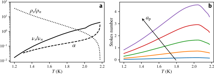
Figure 1: (a) Temperature-dependent properties of superfluid ⁴He. Mutual friction coefficient $\alpha$ from [31], density ratio $\rho_{\text{s}}/\rho_{\text{n}}$ and viscosity ratio $\nu_{\text{s}}/\nu_{\text{n}}$. (b) Dependence of Stokes numbers $\text{St}=\tau_{\text{p}}/\tau_{\eta}^{\text{(n)}}$ on temperature. Stokes numbers are estimated for spherical solid hydrogen particles ($\rho_{\text{p}}/\rho\approx 0.6$ [11]) with diameters ranging from 2 to 10 $\mu$m, using $\tau_{\eta}^{\text{(n)}}={(\rho/\rho_{\text{n}})}^{1/2}\,\tau_{\eta}^{\text{exp}}$ and $\tau_{\eta}^{\text{exp}}=0.1$ ms [32].

II.2 Inertial particles in the HVBK model

Particles in superfluid helium experience a Stokes drag associated to the viscosity of the normal fluid, while also feeling the pressure gradient force from both fluid components. Particles are considered to be much smaller than the Kolmogorov scales of the flow. Hence finite-size effects can be neglected, as well as the action of particles on the flow, since any disturbance of the flow is immediately damped. The Basset history term is also neglected. The equations governing the particle dynamics then read [16, 33]

$$\frac{\text{d}\bm{v}_{\text{p}}}{\text{d}t}=\frac{1}{\tau_{\text{p}}}\left(\bm{u}_{\text{n}}(\bm{x}_{\text{p}})-\bm{v}_{\text{p}}\right)+\beta\left(\frac{\rho_{\text{n}}}{\rho}\frac{\text{D}\bm{u}_{\text{n}}}{\text{D}t}+\frac{\rho_{\text{s}}}{\rho}\frac{\text{D}\bm{u}_{\text{s}}}{\text{D}t}\right)$$ (4)

$$\tau_{\text{p}}=\frac{a_{\text{p}}^{2}}{3\beta\nu},\qquad\beta=\frac{3\rho}{2\rho_{\text{p}}+\rho},$$ (5)

where $\rho_{\text{p}}$ is the particle density and $a_{\text{p}}$ its radius, and $\text{D}/\text{D}t$ are the corresponding material derivatives. The density parameter $\beta$ accounts for added mass effects, while the Stokes time $\tau_{\text{p}}$ represents the particle response time to normal fluid fluctuations. Note that, even though there is a viscous term in Eq. (2), there is no Stokes drag resulting from the superfluid component. Particles moving at velocities close to the speed of sound could in principle trigger vortex nucleations, which would result in an additional effective drag. Here we neglect such small-scale effects.

The superfluid pressure gradient term in Eq. (4), proportional to $\text{D}\bm{u}_{\text{s}}/\text{D}t$, is responsible for particle attraction towards superfluid vortices. Note that the present model does not explicitly account for particles that become trapped by quantum vortices, whose behavior is expected to be different from that of untrapped particles. For instance, in thermal counterflow experiments, trapped particles move towards the heat source along with the superfluid flow, while untrapped ones are transported away from it by the normal component [34]. With regard to the spatial distribution of particles, one can expect that accounting for trapping would further increase the concentration of particles in superfluid vortices compared to the present model.

The Stokes number $\text{St}=\tau_{\text{p}}/\tau_{\eta}^{\text{(n)}}$ quantifies the particle inertia. Here the Kolmogorov time scale associated to the normal component is $\tau_{\eta}^{\text{(n)}}={(\nu_{\text{n}}/\varepsilon_{\text{n}})}^{1/2}$, where $\varepsilon_{\text{n}}$ is the mean energy dissipation rate of the normal fluid. In the limit $\text{St}\to 0$, particles behave as perfect tracers of the normal component. In the opposite limit $\text{St}\to\infty$ the particle motion is ballistic and not modified by turbulent fluctuations. The Stokes numbers of micrometer-sized hydrogen particles based on dissipation measurements in the SHREK experiment [32] are estimated in Fig. 1(b). Remarkably, the temperature dependence of St for fixed particle parameters $(a_{\text{p}},\rho_{\text{p}})$ is non-monotonic due to the variation of helium properties with temperature, and presents a maximum value at $T\approx 2.04\,\text{K}$.

As noted above, the present model is valid in the limit of small particle size compared to the Kolmogorov scale of the normal fluid. In addition, particles should be in principle smaller than the mean inter-vortex distance, so that they do not interact strongly with quantized vortices, and do not get often trapped by them [33]. Consistently with the HVBK approach, which does not explicitly account for quantized vortex dynamics, Eq. (4) should be interpreted as describing the coarse-grained particle dynamics, neglecting the physics at smaller scales. Whether such small-scale phenomena have an impact on the coarse-grained particle dynamics is a challenging question that can only be answered by confronting this model to new experimental results. Note that, in recent superfluid ⁴He experiments, the inter-vortex distance is of order $10\,\mu\text{m}$ [5, 35, 32], comparable both to the Kolmogorov scales and to the typical size of hydrogen particles in experiments.

II.3 Numerical procedure

We investigate the spatial distribution of inertial particles in superfluid ⁴He by numerically solving the HVBK equations (1–3) in a triply periodic box using a parallel pseudo-spectral code (see [36] for details). Point particles are randomly initialized in the domain, and their trajectories are evolved in time until the system reaches a statistically steady state. The time advancement of both particles and fields is performed using a third-order Runge-Kutta scheme. Fluid fields are interpolated at particle positions using fourth-order B-splines [37].

Simulations are performed at temperatures $T=$ 1.3, 1.9 and 2.1 K. Navier-Stokes simulations are also performed for comparison with the classical turbulence case. The number of collocation points in each direction is either $N=$ 256 or 512. Both resolutions only differ on the numerical value of the viscosities $\nu_{\text{n}}$ and $\nu_{\text{s}}$ and on the resulting Reynolds numbers, but the $\nu_{\text{s}}/\nu_{\text{n}}$ ratio is kept the same. The Reynolds numbers associated to the normal and superfluid components are defined as $\text{Re}_{\alpha}=u_{\text{rms}}^{(\alpha)}/(\nu_{\alpha}k_{0})$, where $\alpha=\{\text{n},\text{s}\}$, $u_{\text{rms}}^{(\alpha)}$ is the root-mean-square of the velocity fluctuations, and $1/k_{0}=1$ is the scale of the external forcing. Reynolds numbers are fixed by the resolution, as the smallest scales of the most turbulent component have to be well resolved. For each run, $N_{\text{p}}$ particles of a given class are tracked, each class being defined by a set of parameters $(a_{\text{p}},\rho_{\text{p}})$. Simulation parameters are summarized in Table 1.

Two counterflow simulations (runs IV and V in Table 1) are performed at the temperature $T=1.9\,\text{K}$ at which the two fluid components have comparable properties. The two runs differ on the effective mutual friction force: while the first run uses the same estimate $\Omega_{0}^{2}=\langle|\bm{\omega}_{\text{s}}|^{2}\rangle/2$ as in the coflow runs, the second one takes $\Omega_{0}$ as an external control parameter with a value $4$ times larger than steady value of the first run. The values of $\Omega_{0}$, normalized by $k_{0}u_{\text{rms}}^{\text{(n)}}$ are also displayed in Table 1. Note that effectively, the coupling between the two fluid components is stronger for run V than run IV. As discussed in Sec. II.1, this is to account for a likely underestimation of the mutual friction intensity by the superfluid vorticity-based estimate. This also allows to clarify the effect of the mutual friction on particle concentration statistics. In both cases, the imposed mean counterflow velocity is $U_{\text{ns}}/u_{\text{rms}}^{\text{(n)}}\approx 5$.

Table 1: Simulation parameters. NS denotes Navier-Stokes simulations. (See text for definitions.)

Run	$T$ (K)	$U_{\text{ns}}/u_{\text{rms}}^{\text{(n)}}$	$N$	$\alpha$	$\Omega_{0}/(k_{0}u_{\text{rms}}^{\text{(n)}})$	$\rho_{s}/\rho$	$\rho_{n}/\rho$	$\nu_{s}/\nu_{n}$	$\text{Re}_{\text{n}}$	$\text{Re}_{\text{s}}$	$N_{\text{p}}/10^{6}$
I	1.3	0.0	256	0.034	8.7	0.952	0.048	0.043	28	707	2.0
II		0.0	512		14.2				59	1479	3.2
III	1.9	0.0	256	0.206	7.9	0.574	0.426	1.25	632	516	2.0
IV		4.3	256		2.3				592	426	0.4
V		5.6	256		11.2				447	386	0.4
VI		0.0	512		11.2				1299	1053	3.2
VII	2.1	0.0	256	0.481	7.4	0.259	0.741	2.5	695	268	0.4
VIII		0.0	512		9.8				1332	515	3.2
IX	NS	0.0	256	0.0	–	0.0	1.0	–	780	–	0.4
X		0.0	512		–				1639	–	3.2

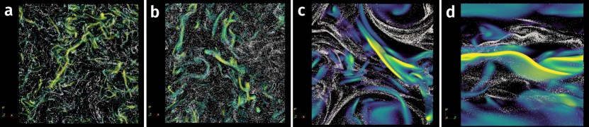
Figure 2: Quasi-two-dimensional slices of the instantaneous particle distribution for $\text{St}=1$ and $\rho_{\text{p}}/\rho=0.7$ ($\beta=1.25$). (a) $T=1.3\,\text{K}$ coflow, run I; (b) $T=1.9\,\text{K}$ coflow, run III; (c–d) $T=1.9\,\text{K}$ counterflow, run IV. In (c), the counterflow direction is normal to the figure. In (d), the counterflow is directed along the horizontal axis. Colors represent regions of high superfluid vorticity.

III Spatial distribution of particles

To illustrate the effect of temperature on particle clustering, we show in Fig. 2 the instantaneous particle distribution obtained from different simulations. Particle parameters are $\text{St}=1$ and $\rho_{\text{p}}/\rho=0.7$, comparable to those typically found in experiments (see Fig. 1b). In turbulent coflow at $T=1.3\,\text{K}$ (Fig. 2a), particles form quasi-one-dimensional clusters that are often aligned with superfluid vortex filaments. At higher temperatures ($T=1.9\,\text{K}$, Fig. 2b), the particle distribution is more uniform, although regions of high particle concentration are still clearly visible. When a mean counterflow is imposed at the same temperature (Fig. 2(c) and (d)), the particle distribution is dominated by the formation of large-scale vortices elongated along the counterflow direction. For the chosen set of parameters, particles tend to escape from such vortices and concentrate in large-scale structures.

Particles in classical turbulence are known to form fractal clusters at distances smaller than the dissipative scale of the flow [38]. A measure of fractal clustering is the correlation dimension $\mathcal{D}_{2}$ [39, 40], estimated as the small-scale power law scaling of the probability $P_{2}(r)$ of finding two particles at a distance smaller than $r$ (i.e. $P_{2}(r)\sim r^{\mathcal{D}_{2}}$ for $r$ small). In three dimensions, $\mathcal{D}_{2}=3$ indicates that particles are uniformly distributed in space, while smaller values are evidence of fractal clustering.

We first consider particles of relative density $\rho_{\text{p}}/\rho=0.7$ at varying particle radius $a_{\text{p}}$. The separation probability $P_{2}(r)$ for different Stokes numbers is shown in Fig. 3(a) for the 1.3 K cases. At small scales, the curves present a clear power law scaling, with an exponent $\mathcal{D}_{2}$ that varies significantly with St. At this temperature, particle clustering is maximal for $\text{St}\approx 0.4$, which would roughly correspond to 6 $\mu$m-diameter hydrogen particles in SHREK (Fig. 1b) or in the Prague oscillating grid experiments [41].

We plot in Fig. 3(b) the correlation dimension $\mathcal{D}_{2}$ from all runs. As in classical turbulence [15], for all temperatures particle clustering is maximal at Stokes numbers of order unity. At temperatures close to $T_{\lambda}$, the minimum value of $\mathcal{D}_{2}$ is close to 2.3, comparable to the case of heavy particles in turbulence [42]. In particular, both counterflow cases at $T=1.9\,\text{K}$ display a maximum clustering at $\text{St}\approx 1$, similarly to the coflow runs at the same temperature. The two counterflow curves nearly collapse, suggesting that there is no significant effect of the mutual friction intensity on $\mathcal{D}_{2}$. As anticipated from Fig. 2, particle clustering changes dramatically in turbulent coflow at lower temperatures. At $T=1.3\,\text{K}$, the minimum value of $\mathcal{D}_{2}$ decreases to 0.75, indicating that particles become concentrated in worm-like structures such as those seen in Fig. 2(a).

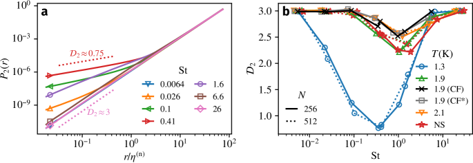
Figure 3: Particle concentration at constant density $\rho_{\text{p}}/\rho=0.7$ ($\beta=1.25$). (a) Separation probability $P_{2}(r)$ for $T=1.3\,\text{K}$ (run II) and for different Stokes numbers. Distances are normalized by the normal component Kolmogorov length scale $\eta^{\text{(n)}}=(\nu_{\text{n}}^{3}/\varepsilon_{\text{n}})^{1/4}$. (b) Correlation dimension $\mathcal{D}_{2}$ as a function of Stokes number for all runs. Different markers represent different cases. CF: counterflow turbulence (run IV). CF*: counterflow turbulence with strong mutual friction (run V). NS: classical turbulence (runs IX, X).

To understand the above observations, we consider the particle equation of motion in the small Stokes number limit ($\tau_{\text{p}}\ll\tau_{\eta}^{\text{(n)}}$). In this case, particles follow an effective compressible velocity field $\bm{v}_{\text{eff}}(\bm{x},t)$ [13, 43]. From Eq. (4), this field writes $\bm{v}_{\text{eff}}\approx\bm{u}_{\text{n}}+\tau_{\text{p}}\left(\beta\frac{\rho_{\text{n}}}{\rho}-1\right)\frac{\text{D}\bm{u}_{\text{n}}}{\text{D}t}+\tau_{\text{p}}\,\beta\frac{\rho_{\text{s}}}{\rho}\frac{\text{D}\bm{u}_{\text{s}}}{\text{D}t}$. Taking its divergence, one finds

$$\frac{1}{\tau_{\text{p}}}\bm{\nabla}\cdot\bm{v}_{\text{eff}}\approx\left(\beta\frac{\rho_{\text{n}}}{\rho}-1\right)(S_{\text{n}}^{2}-\Omega_{\text{n}}^{2})+\beta\frac{\rho_{\text{s}}}{\rho}(S_{\text{s}}^{2}-\Omega_{\text{s}}^{2}),$$ (6)

where $S_{\text{s}}$, $S_{\text{n}}$, $\Omega_{\text{s}}$ and $\Omega_{\text{n}}$ are the norms of the strain-rate and rotation-rate tensors of the two fluids.

In the classical limit where $\rho_{\text{s}}=0$, Eq. (6) indicates that light particles ($\beta>1$) tend to concentrate in vorticity-dominated regions (where $\Omega_{\text{n}}>S_{\text{n}}$), while heavy particles ($\beta<1$) accumulate in strain-dominated regions [44]. For neutral particles ($\beta=1$), the effective velocity field is incompressible and no preferential concentration is expected.

The classical picture changes in low-temperature ⁴He when $\rho_{\text{s}}\gg\rho_{\text{n}}$. In this case, Eq. (6) becomes ${\tau_{\text{p}}}^{-1}\bm{\nabla}\cdot\bm{v}_{\text{eff}}\approx-(S_{\text{n}}^{2}-\Omega_{\text{n}}^{2})+\beta(S_{\text{s}}^{2}-\Omega_{\text{s}}^{2})$, implying that the remaining normal component acts on the particle dynamics only through the Stokes drag. Due to its higher viscosity, the normal velocity field is smoother (has weaker gradients), hence in general $|S_{\text{s}}^{2}-\Omega_{\text{s}}^{2}|\gg|S_{\text{n}}^{2}-\Omega_{\text{n}}^{2}|$. As a consequence, for $\beta$ of order unity, the superfluid term dominates, and thus particles cluster in regions of high superfluid vorticity. We stress that this behavior is unique to quantum turbulence, since the absence of superfluid drag on the particles implies that there is no force counteracting the dominant effect of the superfluid pressure gradient.

In the opposite limit $T\to T_{\lambda}$, the superfluid fraction vanishes and the classical behavior discussed above is recovered. More interesting is the intermediate case where the two fluid densities and viscosities are similar, at $T\approx 1.9\,\text{K}$. In this case, in the absence of a mean counterflow, the two velocity fields are tightly coupled even at the smallest flow scales [24]. Hence, $S_{\text{n}}\approx S_{\text{s}}$ and $\Omega_{\text{n}}\approx\Omega_{\text{s}}$, and the clustering behavior predicted by Eq. (6) falls back to the classical case. This does not apply in the counterflow case, where the normal and superfluid motions are decorrelated at the small scales along the counterflow direction [25].

To support the above predictions and to extend our results to different particle densities, Fig. 4(a) shows $\mathcal{D}_{2}$ as a function of the density parameter $\beta$, for $\text{St}=1$. In the classical case, heavy particles concentrate in planar structures ($\mathcal{D}_{2}\gtrsim 2$) while light particles form localized linear clusters ($\mathcal{D}_{2}\lesssim 1$), consistently with previous findings [45]. For neutral particles, $\mathcal{D}_{2}$ strongly decreases at the lowest temperature, suggesting the formation of linear clusters. The above discussion suggests that these clusters form in high superfluid vorticity regions. This is verified in Fig. 4(b), where the relative enstrophy sampled by the particles, $\mathcal{W}^{\text{p}}_{\alpha}/\mathcal{W}_{\alpha}$ (with $\alpha=\text{n},\text{s}$), is plotted. Here, $\mathcal{W}_{\alpha}=\langle|\bm{\omega}_{\alpha}|^{2}\rangle$ is the enstrophy of a given fluid component (Eulerian average), and $\mathcal{W}^{\text{p}}_{\alpha}=\langle|\bm{\omega}_{\alpha}(\bm{x}_{\text{p}})|^{2}\rangle$ where the average is over particle positions. For $T=1.3\,\text{K}$, neutral and light particles preferentially sample high superfluid vorticity regions.

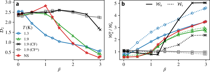
Figure 4: Clustering as a function of particle density for $\text{St}=1$. (a) Correlation dimension $\mathcal{D}_{2}$. (b) Relative enstrophy sampled by the particles, $\mathcal{W}^{\text{p}}_{\alpha}/\mathcal{W}_{\alpha}$, for $\alpha=\text{n},\text{s}$. Solid lines, normal fluid enstrophy; dotted lines, superfluid enstrophy.

We finally discuss the counterflow case. Contrarily to classical and coflowing 3D turbulence, here the two-fluid motion is characterized by large-scale vortices elongated along the counterflow direction and quasi-two-dimensionalization of the flow (as seen in Fig. 2(c-d)), while the small scales are strongly damped due to mutual friction [25]. In contrast with the coflowing case, where the results are strongly dependent on the density parameter $\beta$, here particles form clusters of dimension $\mathcal{D}_{2}\approx 2$ almost regardless of their density (Fig. 4a). This is explained by particles concentrating in sheet-like structures as a result of the two-dimensionalization of the flow. The observed particle organization may explain why quantum vortices are not clearly visualized by particles in some counterflow experiments [46]. Except for the case of very light particles, the mutual friction intensity has virtually no influence on $\mathcal{D}_{2}$, consistently with the observations from Fig. 3(b). This is however not the case for the relative enstrophy sampled by the particles (Fig. 4b), which displays a striking variation with the mutual friction frequency $\Omega_{0}$. In the low $\Omega_{0}$ case, light particles tend to cluster in regions of very high normal fluid vorticity, while this is not the case when $\Omega_{0}$ is increased. This is a consequence of the change of Eulerian fields with the mutual friction intensity. A strong mutual friction results in weaker enstrophy fluctuations in the flow (data not shown). Furthermore, mutual friction suppresses the velocity fluctuations in the counterflow direction [28], enhancing the two-dimensionalization of the flow and thus the formation of vortex sheets that drive particle clustering. This finally explains why the correlation dimension $\mathcal{D}_{2}$ remains close to two when the mutual friction frequency is increased.

IV Summary

We have studied the spatial organization of inertial particles in the HVBK framework for superfluid helium. In the absence of a mean counterflow, the most striking difference with classical fluids is observed at low temperatures when the superfluid mass fraction is dominant. In this case, particles are attracted towards high superfluid vorticity regions regardless of their density relative to the fluid, thus forming quasi-one-dimensional clusters. This attraction is explained by the dominant effect of the superfluid pressure gradient on the particles. At higher temperatures, as the two fluid components become strongly coupled by mutual friction, the classical turbulence behavior is recovered. Namely, light particles concentrate in vortex filaments, while heavy particles are expelled from them. Finally, in the presence of a strong counterflow, the clustering dynamics is governed by the two-dimensionalization of the velocity fields and the formation of large-scale vortex columns or sheets, which either attract or repel particles as a function of the particle density and/or inertia. In this case, particles cluster in quasi-2D structures almost regardless of their density and of the imposed mutual friction intensity.