Center-Outward R-Estimation for
Semiparametric VARMA Models

Abstract

We propose a new class of R-estimators for semiparametric VARMA models in which the innovation density plays the role of the nuisance parameter. Our estimators are based on the novel concepts of multivariate center-outward ranks and signs. We show that these concepts, combined with Le Cam’s asymptotic theory of statistical experiments, yield a class of semiparametric estimation procedures, which are efficient (at a given reference density), root-$n$ consistent, and asymptotically normal under a broad class of (possibly non elliptical) actual innovation densities. No kernel density estimation is required to implement our procedures. A Monte Carlo comparative study of our R-estimators and other routinely-applied competitors demonstrates the benefits of the novel methodology, in large and small sample. Proofs, computational aspects, and further numerical results are available in the supplementary material.

Keywords Multivariate ranks, Distribution-freeness, Local asymptotic normality, Time series, Measure transportation, Quasi likelihood estimation, Skew innovation density.

1 Introduction

1.1 Quasi-maximum likelihood and R-estimation

Gaussian quasi-likelihood methods are pervasive in several areas of statistics. Among them is time series analysis, univariate and multivariate, linear and non-linear. In particular, quasi-maximum likelihood estimation (QMLE)) and correlogram-based testing are the daily practice golden standard for ARMA and VARMA models. They only require the specification of the first two conditional moments, which depend on an unknown Euclidean parameter, while a Gaussian (misspecified) innovation density is assumed. Their properties are generally considered as fully satisfactory: QMLEs, in particular, are root-$n$ consistent, parametrically efficient under Gaussian innovations, and asymptotically normal under finite fourth-order moment assumptions.

Despite their popularity, QMLE methods are not without some undesirable consequences, though, which are often overlooked: (i) while achieving efficiency under Gaussian innovations, their asymptotic performance can be quite poor under non-Gaussian ones; (ii) due to technical reasons (the Fisher consistency requirement), the choice of a quasi-likelihood is always the most pessimistic one: quasi-likelihoods automatically are based on the least favorable innovation density (here, a Gaussian one); (iii) root-$n$ consistency is far from being uniform across innovation densities; (iv) actual fourth-order moments may be infinite.

In principle, the ultimate theoretical remedy to those problems is the semiparametric estimation method described in the monograph by Bickel et al. (1993), which yields uniformly, locally and asymptotically, semiparametrically efficient estimators. For VARMA models, the semiparametric approach does not specify the innovation density (an infinite-dimensional nuisance) and the estimators based on Bickel et al. (1993) methodology are uniformly, locally and asymptotically parametrically efficient (VARMA models are adaptive, thus semiparametric and parametric efficiency coincide). However, semiparametric estimation procedures are not easily implemented, since they rely on kernel-based estimation of the actual innovation density (hence the choice of a kernel, the selection of a bandwidth) and the use of sample splitting techniques. All these niceties require relatively large samples and are hard to put into practice even for univariate time series.

A more flexible and computationally less heavy alternative in the presence of unspecified noise or innovation densities is R-estimation, which reaches efficiency at some chosen reference density (not necessarily Gaussian or least favorable) or class of densities. R-estimation has been proposed first in the context of location (Hodges and Lehmann 1956) and regression models with independent observations (Jurečková 1971, Koul 1971, van Eeden 1972, Jaeckel 1972). Later on, it was extended to autoregressive time series (Koul and Saleh 1993, Koul and Ossiander 1994, Terpstra et al. 2001, Hettmansperger and McKean 2008, Mukherjee and Bai 2002, Andrews 2008, 2012) and non-linear time series (Mukherjee 2007, Andreou and Werker 2015, Hallin and La Vecchia 2017, 2019).

Multivariate extensions of these approaches, however, run into the major difficulty of defining an adequate concept of ranks in the multivariate context. This is most regrettable, as the drawbacks of quasi-likelihood methods for observations in dimension $d=1$ only get worse as the dimension $d$ increases (see Section 1.2 for a numerical example in dimension $d=2$) while the use of the semiparametric method of Bickel et al. becomes problematic: the higher the dimension, the more delicate multivariate kernel density estimation and the larger the required sample size. A natural question is thus: “Can R-estimation palliate the drawbacks of the QMLE and the Bickel et al. technique in dimension $d\geq 2$ the way it does in dimension $d=1$?” This question immediately comes up against another one: “What are ranks and signs, hence, what is R-estimation, in dimension $d\geq 2$?” Indeed, starting with dimension two, the real space $\mathbb{R}^{d}$ is no longer canonically ordered.

The main contribution of this paper is to provide a positive answer to these questions. To this end, we propose a multivariate version of R-estimation, establish its asymptotic properties (root-$n$ consistency and asymptotic normality), and demonstrate its feasibility and excellent finite-sample performance in the context of semiparametric VARMA models. Our approach builds on Chernozhukov et al. (2017), Hallin (2017), and Hallin et al. (2020a), who introduce novel concepts of center-outward ranks and signs based on measure transportation ideas. These center-outward ranks and signs (see Section 3.2 for details) enjoy all the properties that make traditional univariate ranks a successful tool of inference. In particular, they are distribution-free (see Hallin et al. (2020) for details), thus preserve the validity of rank-based procedures irrespective of the possible misspecification of the innovation density. Moreover, they are invariant with respect to shift and global scale factors and equivariant under orthogonal transformations; see Hallin et al. (2020b). Extensive numerical exercises reveal the finite-sample superiority of our R-estimators over the conventional QMLE in the presence of asymmetric innovation densities (skew-normal, skew-$t$, Gaussian mixtures) and in the presence of outliers. All these advantages, however, do not come at the cost of a loss of efficiency under symmetry.

Other notions of multivariate ranks and signs have been proposed in the statistical literature. Among them, the componentwise ranks (Puri and Sen 1971), the spatial ranks (Oja 2010), the depth-based ranks (Liu 1992; Liu and Singh 1993), and the Mahalanobis ranks and signs (Hallin and Paindaveine (2002a)). Those ranks and signs all have their own merits but also some drawbacks, which make them unsuitable for our needs (essentially, they are not distribution-free, or not maximally so); we refer to the introduction of Hallin et al. (2020) for details. The Mahalanobis ranks and signs have been successfully considered for testing purposes in the time series context (Hallin and Paindaveine 2002b, 2004). However, no results on estimation are available, and their distribution-freeness property is limited to elliptical densities—a very strong symmetry assumption which we are dropping here.

Leaving aside Wasserstein-distance-based methods, our contribution constitutes the first inferential application of measure transportation ideas to semiparametric inference for multivariate time series. Measure transportation, which goes back to Gaspard Monge (1746-1818) and his 1781 Mémoire sur la Thérorie des Déblais et des Remblais, in the past few years has become one of the most active and fertile subjects in pure and applied contemporary mathematics. Despite some crucial forerunning contributions (Cuesta-Albertos and Matrán (1997); Rachev and Rüschendorf (1998)), statistics was somewhat slower to join. However, some recent papers on multiple-output quantile regression (Carlier et al. 2016), distribution-free tests of vector independence and multivariate goodness-of-fit (Boeckel et al. (2018); Deb and Sen (2019); Shi et al. (2019); Ghosal and Sen (2019)) demonstrate the growing interest of the statistical community in measure transportation results. We refer to Panaretos and Zemel (2019) for a review.

1.2 A motivating example

As a justification of the practical interest of our R-estimation, let us consider the very simple but highly representative motivating example of a bivariate VAR(1) model

$$\left({\mbox{\boldmath$I$}}_{d}-{\mbox{\boldmath$A$}}L\right){\mbox{\boldmath$X$}}_{t}=\mbox{\boldmath$\epsilon$}_{t},\quad t\in{\mathbb{Z}},$$ (1.1)

with parameter vec$({\mbox{\boldmath$A$}})=:(a_{11},a_{21},a_{12},a_{22})^{\prime}$ taking the value $(0.2,-0.6,0.3,1.1)^{\prime}$. We generated 300 replications of a realization of length $n=1000$ of the stationary solution of (1.1) with two innovation densities—a spherical Gaussian one and a Gaussian mixture (see (5.2) for details)—which both satisfy the conditions for QMLE validity. The resulting boxplots of the QMLE and the Gaussian score (van der Waerden) R-estimator (see Section 4.2 for a definition) are shown in Figure 1, along with the mean squared error (MSE) ratios of the QMLE over the R-estimator.

Even a vary rapid inspection of the plots reveals that, under the mixture distribution, the R-estimator yields sizeably smaller MSE values than the QMLE. For instance, as far as the estimation of $a_{11}$ is concerned, the MSE ratio is 2.657: the R-estimator is strikingly less dispersed than the QMLE. On the other hand, under Gaussian innovations (hence, with the QMLE coinciding with the MLE and achieving parametric efficiency), the QMLE and the R-estimator perform similarly, with MSE ratios extremely close to one for all the parameters. While our R-estimator quite significantly outperforms the QMLE under the mixture distribution, thus, this benefit comes at no cost under Gaussian innovations. Further numerical results are provided in Section 5 and Appendix D; they all lead to the same conclusion.

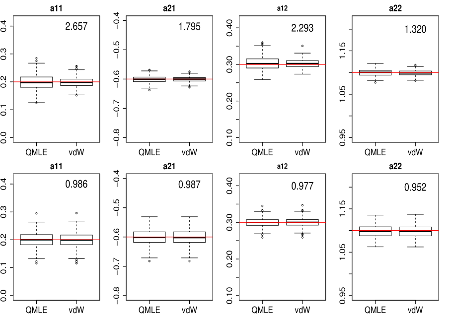
Figure 1: Boxplots of the QMLE and the R-estimator (van der Waerden) of the parameters $a_{11},a_{21},a_{12}$, and $a_{22}$ of the bivariate VAR(1) (1.1) under the Gaussian mixture (5.2) (upper panel) and spherical Gaussian (lower panel) innovation densities, respectively (300 replications of length $n=1000$). In each panel, the MSE ratio of the QMLE with respect to the R-estimator is reported. The horizontal line represents the actual parameter value.

1.3 Outline of the paper

The rest of the paper is organized as follows. Section 2 briefly recalls a local asymptotic normality result for the VARMA model with nonelliptical innovation density: an analytical form of the central sequence as a function of the residuals is provided, which indeed plays a key role in the construction of our estimators. In Section 3, we introduce the measure transportation-based notions of center-outward ranks and signs; for the sake of analogy, we also recall the definition of Mahalanobis ranks and signs, and shortly discuss their respective invariance properties. In Section 3.4, we explain the key idea of our construction of R-estimators, which consists in replacing the residuals appearing in central sequence with some adequate function of their center-outward ranks and signs, yielding a rank-based version of the latter: our R-estimators are obtained by incorporating that rank-based central sequence into a classical Le Cam one-step procedure. Root-$n$ consistency and asymptotic normality are established in Proposition 4.2 under absolutely continuous innovation densities admitting finite second moment. Some standard score functions are discussed in Section 4.2. Section 5 presents simulation results under various densities of the various estimators; comparing their performance confirms the findings of the motivating example of Section 1.2. In Section 6, we show how our R-estimation method applies to a real dataset borrowed from econometrics, where a VARMA($3,1$) model is identified. Finally, Section 7 concludes and provides some perspectives for future research.

All proofs are concentrated in Appendices A and B. Sections 2 and 3 are technical and can be skipped at first reading: the applied statistician can focus directly on the description of one-step R-estimation in (4.8) (implementation details are provided in Appendix C) and the numerical results of Sections 5 and 6 (Appendix D).

2 Local asymptotic normality

Local asymptotic normality (LAN) is an essential ingredient in the construction of our estimators and the derivation of their asymptotic properties. In this section, referring to results by Garel and Hallin (1995) and Hallin and Paindaveine (2004), we state, along with the required assumptions, the LAN property for stationary VARMA models, with an explicit expression for the central sequence to be used later on. The corresponding technical material is available in Appendices A and B.

2.1 Notation and assumptions

We throughout consider the $d$-dimensional VARMA($p,q$) model

$$\Big{(}{\mbox{\boldmath$I$}}_{d}-\sum_{i=1}^{p}{\mbox{\boldmath$A$}}_{i}L^{i}\Big{)}{\mbox{\boldmath$X$}}_{t}=\Big{(}{\mbox{\boldmath$I$}}_{d}+\sum_{j=1}^{q}{\mbox{\boldmath$B$}}_{j}L^{j}\Big{)}\mbox{\boldmath$\epsilon$}_{t},\quad t\in{\mathbb{Z}},\vspace{-2mm}$$ (2.1)

where ${\mbox{\boldmath$A$}}_{1},\ldots,{\mbox{\boldmath$A$}}_{p},{\mbox{\boldmath$B$}}_{1},\ldots,{\mbox{\boldmath$B$}}_{q}$ are $d\times d$ matrices, $L$ is the lag operator, and $\{\mbox{\boldmath$\epsilon$}_{t};t\in{\mathbb{Z}}\}$ is an i.i.d.  mean-zero innovation process with density $f$. The observed series is $\{{\mbox{\boldmath$X$}}^{(n)}_{1},\ldots,{\mbox{\boldmath$X$}}^{(n)}_{n}\}$ (superscript​ ${}^{(n)}\!$ omitted whenever possible) and the $(p+q)d^{2}$-dimensional parameter of interest is

$$\mbox{\boldmath$\theta$}:=\big{(}(\text{vec}{{\mbox{\boldmath$A$}}_{1}})^{\prime},\ldots,(\text{vec}{{\mbox{\boldmath$A$}}_{p}})^{\prime},(\text{vec}{{\mbox{\boldmath$B$}}_{1}})^{\prime},\ldots,(\text{vec}{{\mbox{\boldmath$B$}}_{q}})^{\prime}\big{)}^{\prime},$$

where ^′ indicates transposition. Letting ${\mbox{\boldmath$A$}}(L):={\mbox{\boldmath$I$}}_{d}-\sum_{i=1}^{p}{\mbox{\boldmath$A$}}_{i}L^{i}$, and ${\mbox{\boldmath$B$}}(L):={\mbox{\boldmath$I$}}_{d}+\sum_{j=1}^{q}{\mbox{\boldmath$B$}}_{j}L^{j}$, the following conditions are assumed to hold.

Assumption (A1). (i) All solutions of the determinantal equations

det$$\left({\mbox{\boldmath$I$}}_{d}-\sum_{i=1}^{p}{\mbox{\boldmath$A$}}_{i}z^{i}\right)=0\quad \left({\mbox{\boldmath$I$}}_{d}+\sum_{i=1}^{q}{\mbox{\boldmath$B$}}_{i}z^{i}\right)=0 z\in{\mathbb{C}}$$ and  det,  

lie outside the unit ball in ${\mathbb{C}}$; (ii) $|{\mbox{\boldmath$A$}}_{p}|\neq 0\neq|{\mbox{\boldmath$B$}}_{q}|$; (iii) ${\mbox{\boldmath$I$}}_{d}$ is the greatest common left divisor of ${\mbox{\boldmath$I$}}_{d}-\sum_{i=1}^{p}{\mbox{\boldmath$A$}}_{i}z^{i}$ and ${\mbox{\boldmath$I$}}_{d}+\sum_{i=1}^{q}{\mbox{\boldmath$B$}}_{i}z^{i}$.

Assumption (A1) is standard in the time series literature; the restrictions it imposes on the model parameter ensure the asymptotic stationarity of any solution to (2.1).

To proceed further, we assume that the innovation density $f$ is non-vanishing over ${\mathbb{R}}^{d}$. More precisely we assume that, for all $c\in{\mathbb{R}}^{+}$, there exist constants $b_{c;f}$ and $a_{c;f}$ in $\mathbb{R}$ such that $0<b_{c;f}\leq a_{c;f}<\infty$ and $b_{c;f}\leq f({\mbox{\boldmath$x$}})\leq a_{c;f}$ for $\|{\mbox{\boldmath$x$}}\|\leq c$: denote by ${\cal F}_{d}$ this family of densities.

Assumption (A2). The innovation density $f\in{\cal F}_{d}$ is such that (i) $\int{\mbox{\boldmath$x$}}f({\mbox{\boldmath$x$}})d\mu={\mbox{\boldmath$0$}}$ and the covariance $\mbox{\boldmath$\Xi$}:=\int{\mbox{\boldmath$x$}}{\mbox{\boldmath$x$}}^{\prime}f({\mbox{\boldmath$x$}})d\mu$ is positive definite; (ii) there exists a square-integrable random vector ${\mbox{\boldmath$D$}}f^{1/2}$ such that, for all sequence ${\mbox{\boldmath$h$}}\in\mathbb{R}^{d}$ such that ${\mbox{\boldmath$0$}}\neq{\mbox{\boldmath$h$}}\rightarrow{\mbox{\boldmath$0$}}$,

$$({\mbox{\boldmath$h$}}^{\prime}{\mbox{\boldmath$h$}})^{-1}\int[f^{1/2}({\mbox{\boldmath$x$}}+{\mbox{\boldmath$h$}})-f^{1/2}({\mbox{\boldmath$x$}})-{\mbox{\boldmath$h$}}^{\prime}{\mbox{\boldmath$D$}}f^{1/2}({\mbox{\boldmath$x$}})]^{2}d\mu\rightarrow 0,$$

i.e., $f^{1/2}$ is mean-square differentiable, with mean square gradient ${\mbox{\boldmath$D$}}f^{1/2}$; (iii) letting

$$\mbox{\boldmath$\varphi$}_{f}({\mbox{\boldmath$x$}}):=({\varphi}_{1}({\mbox{\boldmath$x$}}),\ldots,{\varphi}_{d}({\mbox{\boldmath$x$}}))^{\prime}:=-2({\mbox{\boldmath$D$}}f^{1/2})/f^{1/2},$$ (2.2)

$\int{\varphi}_{i}^{4}({\mbox{\boldmath$x$}})f({\mbox{\boldmath$x$}})d\mu<\infty,\ i=1,\ldots,d$; (iv) the score function $\mbox{\boldmath$\varphi$}_{f}$ is piecewise Lipschitz, i.e., there exists a finite measurable partition of ${\mathbb{R}}^{d}$ into $J$ non-overlapping subsets $I_{j}$, $j=1,\ldots,J$ and a constant $K<\infty$ such that $\|\mbox{\boldmath$\varphi$}_{f}({\mbox{\boldmath$x$}})-\mbox{\boldmath$\varphi$}_{f}({\mbox{\boldmath$y$}})\|\leq K\|{\mbox{\boldmath$x$}}-{\mbox{\boldmath$y$}}\|$ for all ${\mbox{\boldmath$x$}},{\mbox{\boldmath$y$}}$ in $I_{j}$, $j=1,\ldots,J$.

Assumption (A2)(i) requires the existence of the second moment of the innovations (a necessary condition for finite VARMA Fisher information). (A2)(ii) is a multivariate version of the classical one-dimensional quadratic mean differentiability assumption on $f^{1/2}$. Together, (A2)(i) and (A2)(iii) imply the existence and finiteness of the Fisher information matrix for location $\mathbfcal{I}(f)=\int\mbox{\boldmath$\varphi$}_{f}({\mbox{\boldmath$x$}})\mbox{\boldmath$\varphi$}_{f}^{\prime}({\mbox{\boldmath$x$}})f({\mbox{\boldmath$x$}})d\mu$ appearing in Proposition 2.1 below. See Garel and Hallin (1995) for further discussion.

Let ${\mbox{\boldmath$Z$}}_{1}^{(n)}(\mbox{\boldmath$\theta$}),\ldots,{\mbox{\boldmath$Z$}}_{n}^{(n)}(\mbox{\boldmath$\theta$})$ denote the residuals computed from the initial values $\mbox{\boldmath$\epsilon$}_{-q+1},\ldots,\mbox{\boldmath$\epsilon$}_{0}$ and ${\mbox{\boldmath$X$}}_{-p+1},\ldots,{\mbox{\boldmath$X$}}_{0}$, the parameter value $\theta$, and the observations ${\mbox{\boldmath$X$}}^{(n)}:=\big{(}{\mbox{\boldmath$X$}}_{1},\ldots,{\mbox{\boldmath$X$}}_{n}\big{)}$; those residuals can be computed recursively, or from (A.1). Clearly, ${\mbox{\boldmath$X$}}^{(n)}$ is the finite realization of a solution of (2.1) with parameter value $\theta$ iff ${\mbox{\boldmath$Z$}}^{(n)}_{1}(\mbox{\boldmath$\theta$}),\ldots,{\mbox{\boldmath$Z$}}^{(n)}_{n}(\mbox{\boldmath$\theta$})$ and $\mbox{\boldmath$\epsilon$}_{1},\ldots,\mbox{\boldmath$\epsilon$}_{n}$ coincide. Denoting by ${\rm P}^{(n)}_{\mbox{\boldmath$\theta$};f}$ the distribution of ${\mbox{\boldmath$X$}}^{(n)}$ under parameter value $\theta$ and innovation density $f$, the residuals ${\mbox{\boldmath$Z$}}_{1}^{(n)}(\mbox{\boldmath$\theta$}),\ldots,{\mbox{\boldmath$Z$}}_{n}^{(n)}(\mbox{\boldmath$\theta$})$ under ${\rm P}^{(n)}_{\mbox{\boldmath$\theta$};f}$ are i.i.d. with density $f$.

2.2 LAN

Writing $L^{(n)}_{\mbox{\boldmath$\theta$}+n^{-1/2}{\mbox{\boldmath$\tau$}}^{(n)}/\mbox{\boldmath$\theta$};f}:=\log{\rm dP}^{(n)}_{\mbox{\boldmath$\theta$}+n^{-1/2}{\mbox{\boldmath$\tau$}}^{(n)};f}/{\rm dP}^{(n)}_{\mbox{\boldmath$\theta$};f}$ for the log-likelihood ratio of ${\rm P}^{(n)}_{\mbox{\boldmath$\theta$}+n^{-1/2}{\mbox{\boldmath$\tau$}}^{(n)};f}$ with respect to ${\rm P}^{(n)}_{\mbox{\boldmath$\theta$};f}$, where ${\mbox{\boldmath$\tau$}}^{(n)}$ is a bounded sequence of $\mathbb{R}^{(p+q)d^{2}}$, let

$$\mbox{\boldmath$\Delta$}^{(n)}_{f}(\mbox{\boldmath$\theta$}):={\mbox{\boldmath$M$}}_{\mbox{\boldmath$\theta$}}^{\prime}{\mbox{\boldmath$P$}}_{\mbox{\boldmath$\theta$}}^{\prime}{\mbox{\boldmath$Q$}}_{\mbox{\boldmath$\theta$}}^{(n)\prime}\mbox{\boldmath$\Gamma$}_{f}^{(n)}(\mbox{\boldmath$\theta$}),\vspace{-1mm}$$ (2.3)

where ${\mbox{\boldmath$M$}}_{\mbox{\boldmath$\theta$}}$, ${\mbox{\boldmath$P$}}_{\mbox{\boldmath$\theta$}}$, and ${\mbox{\boldmath$Q$}}^{(n)}_{\mbox{\boldmath$\theta$}}$ (see (A.2) and (A.3) in Appendix A for an explicit form) do not depend on $f$ nor ${\mbox{\boldmath$\tau$}}^{(n)}$ and

$$\mbox{\boldmath$\Gamma$}_{f}^{(n)}(\mbox{\boldmath$\theta$}):=\big{(}(n-1)^{1/2}(\text{vec}{\mbox{\boldmath$\Gamma$}_{1,f}^{(n)}(\mbox{\boldmath$\theta$})})^{\prime},\ldots,(n-i)^{1/2}(\text{vec}{\mbox{\boldmath$\Gamma$}_{i,f}^{(n)}(\mbox{\boldmath$\theta$})})^{\prime},\ldots,(\text{vec}{\mbox{\boldmath$\Gamma$}_{n-1,f}^{(n)}(\mbox{\boldmath$\theta$})})^{\prime}\big{)}^{\prime}$$ (2.4)

with the so-called $f$-cross-covariance matrices

$$\mbox{\boldmath$\Gamma$}_{i,f}^{(n)}(\mbox{\boldmath$\theta$}):=(n-i)^{-1}\sum_{t=i+1}^{n}\mbox{\boldmath$\varphi$}_{f}({\mbox{\boldmath$Z$}}_{t}^{(n)}(\mbox{\boldmath$\theta$})){\mbox{\boldmath$Z$}}_{t-i}^{(n)\prime}(\mbox{\boldmath$\theta$}).$$ (2.5)

We then have the following LAN result (see Appendix B for a proof).

Proposition 2.1.

Let Assumptions (A1) and (A2) hold. Then, for any bounded sequence ${\mbox{\boldmath$\tau$}}^{(n)}$ in ${\mathbb{R}}^{(p+q)d^{2}}$, under ${\rm P}^{(n)}_{\mbox{\boldmath$\theta$};f}$, as $n\rightarrow\infty$,

$$L^{(n)}_{\mbox{\boldmath$\theta$}+n^{-1/2}{\mbox{\boldmath$\tau$}}^{(n)}/\mbox{\boldmath$\theta$};f}={\mbox{\boldmath$\tau$}}^{{(n)}\prime}\mbox{\boldmath$\Delta$}^{(n)}_{f}(\mbox{\boldmath$\theta$})-\frac{1}{2}{\mbox{\boldmath$\tau$}}^{(n)\prime}\mbox{\boldmath$\Lambda$}_{f}(\mbox{\boldmath$\theta$}){\mbox{\boldmath$\tau$}}^{(n)}+o_{\rm P}(1)\vspace{-1mm}$$ (2.6)

with

$$\mbox{\boldmath$\Lambda$}_{f}(\mbox{\boldmath$\theta$}):={\mbox{\boldmath$M$}}_{\mbox{\boldmath$\theta$}}^{\prime}{\mbox{\boldmath$P$}}_{\mbox{\boldmath$\theta$}}^{\prime}\underset{n\rightarrow\infty}{\lim}\left\{{\mbox{\boldmath$Q$}}_{\mbox{\boldmath$\theta$}}^{(n)\prime}\left[{\mbox{\boldmath$I$}}_{n-1}\otimes\mbox{\boldmath$\Xi$}\otimes\mathbfcal{I}(f)\right]{\mbox{\boldmath$Q$}}_{\mbox{\boldmath$\theta$}}^{(n)}\right\}{\mbox{\boldmath$P$}}_{\mbox{\boldmath$\theta$}}{\mbox{\boldmath$M$}}_{\mbox{\boldmath$\theta$}},$$

and $\mbox{\boldmath$\Delta$}^{(n)}_{f}(\mbox{\boldmath$\theta$})$ is asymptotically normal, with mean $\mathrm{𝟎}$ and variance $\mbox{\boldmath$\Lambda$}_{f}(\mbox{\boldmath$\theta$}))$.

The class ${\cal F}_{d}$ contains, among others, the elliptical densities. Recall that a $d$-dimensional random vector $Z$ has centered elliptical distribution with scatter matrix $\Sigma$ and radial density ${\mathfrak{f}}$ if its density has the form $f({\bf z})=\kappa^{-1}_{d,{\mathfrak{f}}}\big{(}\text{det}{\boldsymbol{\Sigma}}\big{)}^{-1/2}{\mathfrak{f}}\big{(}({\bf z}^{\prime}{\boldsymbol{\Sigma}}^{-1}{\bf z})^{1/2}\big{)}$ for some symmetric positive definite $\boldsymbol{\Sigma}$ and some function $\mathfrak{f}$: $\mathbb{R}^{+}\to\mathbb{R}^{+}$ such that $\int_{0}^{\infty}r^{d-1}{\mathfrak{f}}(r)\,{\mathrm{d}}r<\leavevmode\nobreak\ \!\infty$; $\kappa_{d,{\mathfrak{f}}}:=\big{(}{2\pi^{d/2}}/{\Gamma(d/2)}\big{)}\int_{0}^{\infty}r^{d-1}{\mathfrak{f}}(r)\,{\mathrm{d}}r$ is a norming constant. When $Z$ is elliptical with shape matrix $\boldsymbol{\Sigma}$ and radial density $\mathfrak{f}$, $\|\boldsymbol{\Sigma}^{-1/2}{{\mbox{\boldmath$Z$}}}\|$ (where $\boldsymbol{\Sigma}^{1/2}$ stands for the symmetric root of $\boldsymbol{\Sigma}$) has density ${f}^{\star}_{d;{\mathfrak{f}}}(r)=(\mu_{d-1;{\mathfrak{f}}})^{-1}r^{d-1}\mathfrak{f}(r)I[r>0]$ where $\mu_{d-1;{\mathfrak{f}}}\!:=\!\int_{0}^{\infty}r^{d-1}\mathfrak{f}(r){\rm d}\,r$, and distribution function $F^{\star}_{d;{\mathfrak{f}}}$. Assumption (A2)(ii) on $f$ then is equivalent to the mean square differentiability, with quadratic mean derivative ${\rm D}{\mathfrak{f}}^{1/2}$, of $r\mapsto{\mathfrak{f}}^{1/2}(r)$, $r\in{\mathbb{R}}_{0}^{+}$; letting $\varphi_{\mathfrak{f}}\!:=\!-2{\rm D}{\mathfrak{f}}^{1/2}/{\mathfrak{f}}^{1/2}(r)$, we get ${\cal I}_{d;{\mathfrak{f}}}:=\int_{0}^{1}\!\Big{(}\varphi_{\mathfrak{f}}\circ\big{(}F^{\star}_{d;{\mathfrak{f}}}\big{)}^{-1}\!(u)\Big{)}^{2}{\rm d}u<\leavevmode\nobreak\ \!\infty.$

Elliptic random vectors admit the following representation in terms of spherical uniform variables. Denoting by ${\mathbb{S}}_{d}$ and $\mathcal{S}_{d-1}$ the open unit ball and the unit sphere in $\mathbb{R}^{d}$, respectively, define the spherical uniform distribution ${\rm U}_{d}$ over ${\mathbb{S}}_{d}$ as the product of the uniform measure over $\mathcal{S}_{d-1}$ with a uniform measure over the unit interval of distances to the origin. A $d$-dimensional random vector $Z$ has centered elliptical distribution iff $F^{\star}_{d;{\mathfrak{f}}}(\|\mbox{\boldmath$\Sigma$}^{-1/2}{\mbox{\boldmath$Z$}}\|)\mbox{\boldmath$\Sigma$}^{-1/2}{\mbox{\boldmath$Z$}}/\|\mbox{\boldmath$\Sigma$}^{-1/2}{\mbox{\boldmath$Z$}}\|\sim{\rm U}_{d}$. Putting ${\mbox{\boldmath$S$}}_{\mbox{\boldmath$\Sigma$},t}^{(n)}:=\mbox{\boldmath$\Sigma$}^{-1/2}{\mbox{\boldmath$Z$}}^{(n)}_{t}/\|\mbox{\boldmath$\Sigma$}^{-1/2}{\mbox{\boldmath$Z$}}^{(n)}_{t}\|$, where ${\mbox{\boldmath$Z$}}^{(n)}_{t}:={\mbox{\boldmath$Z$}}^{(n)}_{t}(\mbox{\boldmath$\theta$})$, it follows from Hallin and Paindaveine (2004) that the central sequence (2.3) for elliptical $f$ considerably simplifies and takes the form (2.3) with

$$\mbox{\boldmath$\Gamma$}_{i,f}^{(n)}(\mbox{\boldmath$\theta$}):=(n-i)^{-1}\mbox{\boldmath$\Sigma$}^{-1/2}\sum_{t=i+1}^{n}{\varphi}_{1}(\|\mbox{\boldmath$\Sigma$}^{-1/2}{\mbox{\boldmath$Z$}}^{(n)}_{t}\|){\varphi}_{2}(\|\mbox{\boldmath$\Sigma$}^{-1/2}{\mbox{\boldmath$Z$}}^{(n)}_{t-i}\|){\mbox{\boldmath$S$}}_{\mbox{\boldmath$\Sigma$},t}^{(n)}{\mbox{\boldmath$S$}}^{(n)\prime}_{\mbox{\boldmath$\Sigma$},t-i}\mbox{\boldmath$\Sigma$}^{1/2}\vspace{-1mm}$$ (2.7)

where ${\varphi}_{1}(r):={\varphi}_{\mathfrak{f}}(r)$ and ${\varphi}_{2}(r):=r$, $r\in\mathbb{R}^{+}$.

3 Center-outward ranks and signs

Parametrically optimal (in the Hájek-Le Cam asymptotic sense) rank-based inference procedures in LAN families is possible if the LAN central sequence can be expressed in terms of signs and ranks. In Section 3.4, we explain how to achieve this goal using the notions of multivariate ranks and signs proposed by Chernozhukov et al. (2017) (under the name of Monge-Kantorovich ranks and signs) and developed in Hallin (2017) and Hallin et al. (2020a) under the name of center-outward ranks and signs. This new concepts hinge on measure transportation theory; their empirical versions are based on an optimal coupling of the sample residuals ${\bf Z}^{(n)}_{t}$ with a regular grid over the unit ball.

3.1 Mapping the residuals to the unit ball

Let $\mathcal{P}_{d}$ denote the family of all distributions $\rm P$ with densities in ${\mathcal{F}}_{d}$—for this family the center-outward distribution functions defined below are continuous; see Hallin et al. (2020a). The center-outward distribution function ${\mbox{\boldmath$F$}}_{{\mspace{-1.0mu}{\scriptscriptstyle\pm}}}$ is defined as the a.e. unique gradient of convex function mapping ${\mathbb{R}}^{d}$ to $\mathbb{S}_{d}$ and pushing $\rm P$ forward to ${\rm U}_{d}$. For ${\rm P}\in{\mathcal{P}}_{d}$, such mapping is a homeomorphism between ${\mathbb{S}}_{d}\setminus\{{\bf 0}\}$ and $\mathbb{R}^{d}\setminus{\mbox{\boldmath$F$}}_{{\mspace{-1.0mu}{\scriptscriptstyle\pm}}}^{-1}(\{{\bf 0}\})$ (Figalli 2018) and the corresponding center-outward quantile function is defined (letting, with a small abuse of notation, ${\mbox{\boldmath$Q$}}_{\mspace{-1.0mu}{\scriptscriptstyle\pm}}({\bf 0}):={\mbox{\boldmath$F$}}_{\mspace{-1.0mu}{\scriptscriptstyle\pm}}^{-1}(\{{\bf 0}\})$) as ${\mbox{\boldmath$Q$}}_{\mspace{-1.0mu}{\scriptscriptstyle\pm}}:={\mbox{\boldmath$F$}}_{\mspace{-1.0mu}{\scriptscriptstyle\pm}}^{-1}$. For any given distribution $\rm P$, ${\mbox{\boldmath$Q$}}_{{\mspace{-1.0mu}{\scriptscriptstyle\pm}}}$ induces a collection of continuous, connected, and nested quantile contours and regions; the center-outward median ${\mbox{\boldmath$Q$}}_{\mspace{-1.0mu}{\scriptscriptstyle\pm}}({\mbox{\boldmath$0$}})$ is a uniquely defined compact set of Lebesgue measure zero. We refer to Hallin et al. (2020a) for details.

Turning to the sample, for any $\mbox{\boldmath$\theta$}\in\boldsymbol{\Theta}$, the residuals ${\mbox{\boldmath$Z$}}^{(n)}(\mbox{\boldmath$\theta$})\!:=\!({\mbox{\boldmath$Z$}}_{1}^{(n)}(\mbox{\boldmath$\theta$}),\ldots,{\mbox{\boldmath$Z$}}_{n}^{(n)}(\mbox{\boldmath$\theta$}))$ under ${\rm P}^{(n)}_{\mbox{\boldmath$\theta$};f}$ are i.i.d. with density $f\in{\cal F}_{d}$ and center-outward distribution function ${\mbox{\boldmath$F$}}_{\mspace{-1.0mu}{\scriptscriptstyle\pm}}$. For the empirical counterpart ${\mbox{\boldmath$F$}}^{(n)}_{\mspace{-1.0mu}{\scriptscriptstyle\pm}}$ of ${\mbox{\boldmath$F$}}_{\mspace{-1.0mu}{\scriptscriptstyle\pm}}$, let $n$ factorize into $n=n_{R}n_{S}+n_{0},$ for $n_{R},n_{S},n_{0}\in\mathbb{N}$ and $0\leq n_{0}<\min\{n_{R},n_{S}\}$, where $n_{R}\rightarrow\infty$ and $n_{S}\rightarrow\infty$ as $n\rightarrow\infty$, and consider a sequence of grids, where each grid consists of the intersection between an $n_{S}$-tuple $(\boldsymbol{u}_{1},\ldots\boldsymbol{u}_{n_{S}})$ of unit vectors, and the $n_{R}$-hyperspheres centered at the origin, with radii $1/(n_{R}+1),\ldots,n_{R}/(n_{R}+1)$, along with $n_{0}$ copies of the origin. The resulting grid is such that the discrete distribution with probability mass $1/n$ at each gridpoint and probability mass $n_{0}/n$ at the origin converges weakly to the uniform ${\rm U}_{d}$ over the ball $\mathbb{S}_{d}$. Then, we define ${\mbox{\boldmath$F$}}_{{\mspace{-1.0mu}{\scriptscriptstyle\pm}}}^{(n)}({\mbox{\boldmath$Z$}}^{(n)}_{t})$, for $t=1,\ldots,n$ as the solution (optimal mapping) of a coupling problem between the residuals and the grid.

Specifically, the empirical center-outward distribution function is the (random) mapping

$${\mbox{\boldmath$F$}}^{(n)}_{{\mspace{-1.0mu}{\scriptscriptstyle\pm}}}:{\mbox{\boldmath$Z$}}^{(n)}:=({\mbox{\boldmath$Z$}}^{(n)}_{1},\ldots,{\mbox{\boldmath$Z$}}^{(n)}_{n})\mapsto({\mbox{\boldmath$F$}}^{(n)}_{{\mspace{-1.0mu}{\scriptscriptstyle\pm}}}({\mbox{\boldmath$Z$}}^{(n)}_{1}),\ldots,{\mbox{\boldmath$F$}}^{(n)}_{{\mspace{-1.0mu}{\scriptscriptstyle\pm}}}({\mbox{\boldmath$Z$}}^{(n)}_{n}))$$

satisfying

$$\sum_{t=1}^{n}\|{\mbox{\boldmath$Z$}}^{(n)}_{t}-{\mbox{\boldmath$F$}}^{(n)}_{\mspace{-1.0mu}{\scriptscriptstyle\pm}}({\mbox{\boldmath$Z$}}^{(n)}_{t})\|^{2}=\underset{T\in\mathcal{T}}{\min}\sum_{t=1}^{n}\|{\mbox{\boldmath$Z$}}^{(n)}_{t}-T({\mbox{\boldmath$Z$}}^{(n)}_{t})\|^{2},$$ (3.1)

where ${\mbox{\boldmath$Z$}}^{(n)}_{t}={\mbox{\boldmath$Z$}}^{(n)}_{t}(\mbox{\boldmath$\theta$})$, the set $\{{\mbox{\boldmath$F$}}^{(n)}_{{\mspace{-1.0mu}{\scriptscriptstyle\pm}}}({\mbox{\boldmath$Z$}}^{(n)}_{t})|t=1,\ldots,n\}$ coincides with the $n$ points of the grid, and $\mathcal{T}$ denotes the set of all possible bijective mappings between ${\mbox{\boldmath$Z$}}^{(n)}_{1},\ldots,{\mbox{\boldmath$Z$}}^{(n)}_{n}$ and the $n$ grid points. The sample counterpart of ${\mbox{\boldmath$Q$}}_{\mspace{-1.0mu}{\scriptscriptstyle\pm}}$ then is defined as ${\mbox{\boldmath$Q$}}^{(n)}_{\mspace{-1.0mu}{\scriptscriptstyle\pm}}:=({\mbox{\boldmath$F$}}_{{\mspace{-1.0mu}{\scriptscriptstyle\pm}}}^{(n)})^{-1}$ (again, with the small abuse of notation ${\mbox{\boldmath$Q$}}^{(n)}_{\mspace{-1.0mu}{\scriptscriptstyle\pm}}({\bf 0}):=({\mbox{\boldmath$F$}}_{{\mspace{-1.0mu}{\scriptscriptstyle\pm}}}^{(n)})^{-1}(\{{\bf 0}\})$). See Appendix D.1 for a graphical illustration of these concepts.

Based on this empirical center-outward distribution function, the center-outward ranks and signs are

$${R^{(n)}_{{\mspace{-1.0mu}{\scriptscriptstyle\pm}},t}}:={R^{(n)}_{{\mspace{-1.0mu}{\scriptscriptstyle\pm}},t}}(\mbox{\boldmath$\theta$}):=({n_{R}+1})\|{\mbox{\boldmath$F$}}^{(n)}_{\mspace{-1.0mu}{\scriptscriptstyle\pm}}({\mbox{\boldmath$Z$}}^{(n)}_{t})\|,$$ (3.2)

and (for ${\mbox{\boldmath$F$}}^{(n)}_{\mspace{-1.0mu}{\scriptscriptstyle\pm}}({\mbox{\boldmath$Z$}}^{(n)}_{t})=\boldsymbol{0}$, let ${\mbox{\boldmath$S$}}^{(n)}_{{\mspace{-1.0mu}{\scriptscriptstyle\pm}},t}:=\boldsymbol{0}$)

$${\mbox{\boldmath$S$}}^{(n)}_{{\mspace{-1.0mu}{\scriptscriptstyle\pm}},t}:={{\mbox{\boldmath$S$}}^{(n)}_{{\mspace{-1.0mu}{\scriptscriptstyle\pm}},t}}(\mbox{\boldmath$\theta$}):=\frac{{\mbox{\boldmath$F$}}^{(n)}_{\mspace{-1.0mu}{\scriptscriptstyle\pm}}({\mbox{\boldmath$Z$}}^{(n)}_{t})}{\|{\mbox{\boldmath$F$}}^{(n)}_{\mspace{-1.0mu}{\scriptscriptstyle\pm}}({\mbox{\boldmath$Z$}}^{(n)}_{t})\|}I[{\mbox{\boldmath$F$}}^{(n)}_{\mspace{-1.0mu}{\scriptscriptstyle\pm}}({\mbox{\boldmath$Z$}}^{(n)}_{t})\neq\boldsymbol{0}],\vspace{-2mm}$$ (3.3)

respectively. It follows that ${\mbox{\boldmath$F$}}^{(n)}_{\mspace{-1.0mu}{\scriptscriptstyle\pm}}({\mbox{\boldmath$Z$}}_{t}^{(n)})$ factorizes into

$${\mbox{\boldmath$F$}}^{(n)}_{\mspace{-1.0mu}{\scriptscriptstyle\pm}}({\mbox{\boldmath$Z$}}_{t}^{(n)})=\frac{R^{(n)}_{{\mspace{-1.0mu}{\scriptscriptstyle\pm}},t}}{n_{R}+1}{\mbox{\boldmath$S$}}^{(n)}_{{\mspace{-1.0mu}{\scriptscriptstyle\pm}},t},\quad\text{ hence }\quad{\mbox{\boldmath$Z$}}_{t}^{(n)}={\mbox{\boldmath$Q$}}^{(n)}_{\mspace{-1.0mu}{\scriptscriptstyle\pm}}\Big{(}\frac{R^{(n)}_{{\mspace{-1.0mu}{\scriptscriptstyle\pm}},t}}{n_{R}+1}{\mbox{\boldmath$S$}}^{(n)}_{{\mspace{-1.0mu}{\scriptscriptstyle\pm}},t}\Big{)}.$$ (3.4)

Conditional on the grid (in case the latter is random), those ranks and signs are jointly distribution-free: more precisely, under ${\rm P}^{(n)}_{\mbox{\boldmath$\theta$};f}$, the $n$-tuple ${\mbox{\boldmath$F$}}^{(n)}_{\mspace{-1.0mu}{\scriptscriptstyle\pm}}({\mbox{\boldmath$Z$}}_{1}^{(n)}),\ldots,{\mbox{\boldmath$F$}}^{(n)}_{\mspace{-1.0mu}{\scriptscriptstyle\pm}}({\mbox{\boldmath$Z$}}_{n}^{(n)})$ is uniformly distributed over the $n!$ permutations of the $n$ gridpoints, irrespective of $f\in{\cal F}_{d}$.

We refer to Sections 3.1 and 6 in Hallin et al. (2020a) for further details, comments on the main properties of ${\mbox{\boldmath$F$}}^{(n)}_{\mspace{-1.0mu}{\scriptscriptstyle\pm}}$ and ${\mbox{\boldmath$F$}}_{\mspace{-1.0mu}{\scriptscriptstyle\pm}}$, and for remarks on the sufficiency and maximal ancillarity of the sub-$\sigma$-fields generated by the order statistic and by the center-outward ranks and signs, in the fixed-$\theta$ experiment $\{{\rm P}^{(n)}_{\mbox{\boldmath$\theta$};f}|f\in{\mathcal{F}}_{d}\}$.

3.2 Mahalanobis ranks and signs

Definitions (3.2) and (3.3) call for a comparison with the earlier concepts of elliptical or Mahalanobis ranks and signs introduced in Hallin and Paindaveine (2002a and b, 2004), which we now describe. Associated with the centered elliptical distribution with scatter $\Sigma$ and radial density $\mathfrak{f}$, consider the mapping ${\mbox{\boldmath$z$}}\mapsto{{\mbox{\boldmath$F$}}}_{\text{\tiny\!{\rm ell}}}({\mbox{\boldmath$z$}}):=F^{\star}_{d;\mathfrak{f}}(\|\mbox{\boldmath$\Sigma$}^{-1/2}{\mbox{\boldmath$z$}}\|)\mbox{\boldmath$\Sigma$}^{-1/2}{\mbox{\boldmath$z$}}/\|\mbox{\boldmath$\Sigma$}^{-1/2}{\mbox{\boldmath$z$}}\|$ from $\mathbb{R}^{d}$ to ${\mathbb{S}}_{d}$. In measure transportation parlance, ${{\mbox{\boldmath$F$}}}_{\text{\tiny\!{\rm ell}}}$, just as ${{\mbox{\boldmath$F$}}}_{\mspace{-1.0mu}{\scriptscriptstyle\pm}}$, pushes the elliptical distribution of $Z$ forward to the uniform ${\rm U}_{d}$ over the unit ball ${\mathbb{S}}_{d}$. This allows us to connect the Mahalanobis ranks and signs to the center-outward ones.

Denoting by $\widehat{\mbox{\boldmath$\Sigma$}}^{(n)}$ a consistent estimator of $\Sigma$ measurable with respect to the order statistic of the ${\mbox{\boldmath$Z$}}^{(n)}_{t}$’s and by $F^{\star(n)}$ the empirical distribution function of the moduli $\big{\|}\big{(}\widehat{\mbox{\boldmath$\Sigma$}}^{(n)}\big{)}^{-1/2}{\mbox{\boldmath$Z$}}^{(n)}_{t}\big{\|}$, an empirical counterpart of ${{\mbox{\boldmath$F$}}}_{\text{\tiny\!{\rm ell}}}({\mbox{\boldmath$Z$}}^{(n)}_{t})$ is

$${{\mbox{\boldmath$F$}}}^{(n)}_{\text{\tiny\!{\rm ell}}}({\mbox{\boldmath$Z$}}^{(n)}_{t}):=F^{\star(n)}\big{(}\big{\|}\big{(}\widehat{\mbox{\boldmath$\Sigma$}}^{(n)}\big{)}^{-1/2}{\mbox{\boldmath$Z$}}^{(n)}_{t}\big{\|}\big{)}\frac{\big{(}\widehat{\mbox{\boldmath$\Sigma$}}^{(n)}\big{)}^{-1/2}{\mbox{\boldmath$Z$}}^{(n)}_{t}}{\big{\|}\big{(}\widehat{\mbox{\boldmath$\Sigma$}}^{(n)}\big{)}^{-1/2}{\mbox{\boldmath$Z$}}^{(n)}_{t}\big{\|}}\vspace{-2mm}$$ (3.5)

with the Mahalanobis ranks (compare to (3.2))

$$R^{(n)}_{\text{ell},t}:=R^{(n)}_{\text{ell},t}(\mbox{\boldmath$\theta$}):=(n+1)\|{{\mbox{\boldmath$F$}}}^{(n)}_{\text{\tiny\!{\rm ell}}}({\mbox{\boldmath$Z$}}^{(n)}_{t})\|=(n+1)F^{\star(n)}\big{(}\big{\|}\big{(}\widehat{\mbox{\boldmath$\Sigma$}}^{(n)}\big{)}^{-1/2}{\mbox{\boldmath$Z$}}^{(n)}_{t}\big{\|}\big{)}$$ (3.6)

and Mahalanobis signs (compare to (3.3))

$${\mbox{\boldmath$S$}}^{(n)}_{\text{ell},t}:={\mbox{\boldmath$S$}}^{(n)}_{\text{ell},t}(\mbox{\boldmath$\theta$}):=\frac{{\mbox{\boldmath$F$}}^{(n)}_{\text{\tiny\!{\rm ell}}}({\mbox{\boldmath$Z$}}^{(n)}_{t})}{\|{\mbox{\boldmath$F$}}^{(n)}_{\text{\tiny\!{\rm ell}}}({\mbox{\boldmath$Z$}}^{(n)}_{t})\|}I[{\mbox{\boldmath$F$}}^{(n)}_{\text{\tiny\!{\rm ell}}}({\mbox{\boldmath$Z$}}^{(n)}_{t})\neq\boldsymbol{0}]=\frac{\big{(}\widehat{\mbox{\boldmath$\Sigma$}}^{(n)}\big{)}^{-1/2}{\mbox{\boldmath$Z$}}^{(n)}_{t}}{\big{\|}\big{(}\widehat{\mbox{\boldmath$\Sigma$}}^{(n)}\big{)}^{-1/2}{\mbox{\boldmath$Z$}}^{(n)}_{t}\big{\|}}I\big{[}\big{(}\widehat{\mbox{\boldmath$\Sigma$}}^{(n)}\big{)}^{-1/2}{\mbox{\boldmath$Z$}}^{(n)}_{t}\neq\boldsymbol{0}\big{]}$$ (3.7)

(for ${\mbox{\boldmath$F$}}^{(n)}_{\text{\tiny\!{\rm ell}}}({\mbox{\boldmath$Z$}}^{(n)}_{t})=\boldsymbol{0}=\big{(}\widehat{\mbox{\boldmath$\Sigma$}}^{(n)}\big{)}^{-1/2}{\mbox{\boldmath$Z$}}^{(n)}_{t}$, let ${\mbox{\boldmath$S$}}^{(n)}_{\text{ell},t}:=\boldsymbol{0}$). Similar to (3.4)), we have

$${\mbox{\boldmath$F$}}^{(n)}_{\text{\tiny\!{\rm ell}}}({\mbox{\boldmath$Z$}}_{t}^{(n)})=\frac{R^{(n)}_{\text{ell},t}}{n+1}{\mbox{\boldmath$S$}}^{(n)}_{\text{ell},t},\quad\!\!\text{hence}\!\!\quad\widehat{\mbox{\boldmath$\Sigma$}}^{(n)-1/2}{\mbox{\boldmath$Z$}}_{t}^{(n)}\!=(F^{\star(n)})^{-1}\!\left(\frac{R^{(n)}_{\text{ell},t}}{n+1}\right){\mbox{\boldmath$S$}}^{(n)}_{\text{ell},t}={\mbox{\boldmath$\Sigma$}}^{-1/2}{\mbox{\boldmath$Z$}}_{t}^{(n)}+o_{\mathrm{P}}(1).\vspace{-1mm}$$

3.3 Elliptical ${{\mbox{\boldmath$F$}}}_{\text{\tiny\!{\rm ell}}}$, center-outward ${{\mbox{\boldmath$F$}}}_{\mspace{-1.0mu}{\scriptscriptstyle\pm}}$, and affine invariance

Both ${{\mbox{\boldmath$F$}}}_{\text{\tiny\!{\rm ell}}}$ and ${{\mbox{\boldmath$F$}}}_{\mspace{-1.0mu}{\scriptscriptstyle\pm}}$ are pushing the elliptical distribution of $Z$ forward to ${\rm U}_{d}$. However, unless $\boldsymbol{\Sigma}$ is proportional to identity ($\mbox{\boldmath$\Sigma$}=c{\mbox{\boldmath$I$}}_{d}$ for some $c>0$), ${{\mbox{\boldmath$F$}}}_{\text{\tiny\!{\rm ell}}}$ and ${{\mbox{\boldmath$F$}}}_{\mspace{-1.0mu}{\scriptscriptstyle\pm}}$ are distinct, so that ${{\mbox{\boldmath$F$}}}_{\text{\tiny\!\! {\rm ell}}}$ cannot be the gradient of a convex function. Moreover, both ${{\mbox{\boldmath$F$}}}_{\text{\tiny\!{\rm ell}}}$ and ${{\mbox{\boldmath$F$}}}_{\mspace{-1.0mu}{\scriptscriptstyle\pm}}$ sphericize the distribution of $Z$. Some key differences are worth to be mentioned, though.

First, while sphericization and probability integral transformation, in ${{\mbox{\boldmath$F$}}}_{\mspace{-1.0mu}{\scriptscriptstyle\pm}}$, are inseparably combined, ${{\mbox{\boldmath$F$}}}_{\text{\tiny\!{\rm ell}}}$ proceeds in two separate steps: a Mahalanobis sphericization step (the parametric affine transformation ${\mbox{\boldmath$z$}}\mapsto{\mbox{\boldmath$z$}}_{\mbox{\boldmath$\Sigma$},\boldsymbol{\mu}}:={\mbox{\boldmath$\Sigma$}}^{-1/2}({\mbox{\boldmath$z$}}-\boldsymbol{\mu}$)) first, followed by the spherical probability integral transformation ${\mbox{\boldmath$z$}}_{{\mbox{\boldmath$\Sigma$},\boldsymbol{\mu}}}\mapsto F^{\star}_{d;{\mathfrak{f}}}(\|{\mbox{\boldmath$z$}}_{{\mbox{\boldmath$\Sigma$},\boldsymbol{\mu}}}\|){\mbox{\boldmath$z$}}_{{\mbox{\boldmath$\Sigma$},\boldsymbol{\mu}}}/\|{\mbox{\boldmath$z$}}_{{\mbox{\boldmath$\Sigma$},\boldsymbol{\mu}}}\|$.

Second, Mahalanobis sphericization requires centering, hence the definition of a location parameter $\boldsymbol{\mu}$. Distinct choices of location (mean, spatial median, etc.) all yield the same result under ellipticity, but not under non-elliptical distributions. This is in sharp contrast with ${{\mbox{\boldmath$F$}}}_{\mspace{-1.0mu}{\scriptscriptstyle\pm}}$, which is location-invariant (see Hallin et al. (2020b)). Similarly, all definitions and sensible estimators of the scatter yield the same results under elliptical symmetry but not under non-elliptical distributions.

Third, even under additional assumptions ensuring the identification of $\boldsymbol{\Sigma}$, the Mahalanobis sphericization, hence also ${{\mbox{\boldmath$F$}}}_{\text{\tiny\!{\rm ell}}}$, only sphericizes elliptical distributions, whilst ${{\mbox{\boldmath$F$}}}_{\mspace{-1.0mu}{\scriptscriptstyle\pm}}$ sphericizes them all.

Its preliminary Mahalanobis sphericization step actually makes ${{\mbox{\boldmath$F$}}}_{\text{\tiny\!{\rm ell}}}$ affine-invariant. Assuming that sensible choices of $\boldsymbol{\mu}$ and $\boldsymbol{\Sigma}$ are available, performing the same Mahalanobis transformation prior to determining ${{\mbox{\boldmath$F$}}}_{\mspace{-1.0mu}{\scriptscriptstyle\pm}}$ similarly would make center-outward distribution functions affine-invariant and the corresponding center-outward quantile functions affine-equivariant (in fact, for elliptical distributions, the resulting ${{\mbox{\boldmath$F$}}}_{\mspace{-1.0mu}{\scriptscriptstyle\pm}}$ then coincides with ${{\mbox{\boldmath$F$}}}_{\text{\tiny\!{\rm ell}}}$). Whether this is desirable is a matter of choice. While affine-invariance, in view of the central role of the affine group in elliptical families, is quite natural under elliptical symmetry, its relevance is much less obvious away from ellipticity. A more detailed discussion of this fact, along with additional arguments related to the lack of affine invariance of non-elliptical local experiments, can be found in Hallin et al. (2020b).

Besides affine invariance issues, center-outward distribution functions, ranks, and signs inherit, from the invariance properties of Euclidean distances, elementary but remarkable invariance and equivariance properties: as shown in Hallin et al. (2020b) they enjoy invariance/equivariance with respect to shift, global scale factors, and orthogonal transformations.

3.4 A center-outward sign- and rank-based central sequence

Efficient estimation in LAN experiments is based on central sequences and the so-called Le Cam one-step method. Our R-estimation is based on the same principles. Specifically, in the central sequence associated with some reference density $f$, we replace the residuals ${\mbox{\boldmath$Z$}}(\mbox{\boldmath$\theta$})$ with some adequate function of their ranks and their signs. Then, from the resulting rank-based statistic, we implement a suitable adaptation of the one-step method. If, under innovation density $f$, the substitution yields a genuinely rank-based, hence distribution-free, version of the central sequence, the resulting R-estimator achieves parametric efficiency under $f$ while remaining valid under other innovation densities; see Hallin and Werker (2003) for a discussion.

In dimension $d=1$, Allal et al. (2001), Hallin and La Vecchia (2017, 2019 and references therein) explain how to construct R-estimators for linear and nonlinear semiparametric time series models. In dimension $d>1$, under elliptical innovations density, Hallin et al. (2006) exploit similar ideas for the estimation of shape matrices, based on the Mahalanobis ranks and signs. Hallin and Paindaveine (2004), in a hypothesis testing context, show that replacing ${\bf Z}^{(n)}_{t}$ in (2.7) with

$$\widehat{\mbox{\boldmath$\Sigma$}}^{(n)1/2}F^{\star-1}_{d;{\mathfrak{f}}}(R^{(n)}_{\text{ell},t}/(n+1)){\mbox{\boldmath$S$}}^{(n)}_{\text{ell},t}={\mbox{\boldmath$F$}}_{\text{\tiny\!{\rm ell}}}^{-1}((R^{(n)}_{\text{ell},t}/(n+1)){\mbox{\boldmath$S$}}^{(n)}_{\text{ell},t})={\mbox{\boldmath$F$}}_{\text{\tiny\!{\rm ell}}}^{-1}({\mbox{\boldmath$F$}}^{(n)}_{\text{\tiny\!{\rm ell}}}({\mbox{\boldmath$Z$}}_{t}^{(n)}(\mbox{\boldmath$\theta$})))$$ (3.8)

(where $R^{(n)}_{\text{ell},t}=R^{(n)}_{\text{ell},t}(\mbox{\boldmath$\theta$})$, ${\mbox{\boldmath$S$}}^{(n)}_{\text{ell},t}={\mbox{\boldmath$S$}}^{(n)}_{\text{ell},t}(\mbox{\boldmath$\theta$})$, and $\widehat{\mbox{\boldmath$\Sigma$}}^{(n)}$ is a suitable estimator of the scatter matrix) yields a rank-based version of the central sequence associated with the elliptic density $f$—namely, a random vector $\stackunder[1pt]{\mbox{\boldmath$\Delta$}}{\scriptscriptstyle\thicksim}^{(n)}_{f}(\mbox{\boldmath$\theta$})$ measurable with respect to the Mahalanobis ranks and signs (hence, distribution-free under ellipticity) such that, under $f$, $\stackunder[1pt]{\mbox{\boldmath$\Delta$}}{\scriptscriptstyle\thicksim}^{(n)}_{f}(\mbox{\boldmath$\theta$})-\mbox{\boldmath$\Delta$}^{(n)}_{f}(\mbox{\boldmath$\theta$})$ is $o_{\rm P}(1)$ as $n\to\infty$.

However, this construction is valid only for the family of elliptical innovation densities (in dimension one, the family of symmetric innovation densities), under which Mahalanobis ranks and signs are distribution-free. This is a severe limitation, which is unlikely to be satisfied in most applications. If the attractive properties of R-estimators in univariate semiparametric time series models are to be extended to dimension two and higher, center-outward ranks and signs, the distribution-freeness of which holds under any density $f\in{\cal F}_{d}$, are to be considered instead of the Mahalanobis ones.

Building on this remark, we propose to substitute ${\mbox{\boldmath$Z$}}^{(n)}_{t}(\mbox{\boldmath$\theta$})$ in (2.5) with

$${\mbox{\boldmath$F$}}_{\mspace{-1.0mu}{\scriptscriptstyle\pm}}^{-1}(({R^{(n)}_{{\mspace{-1.0mu}{\scriptscriptstyle\pm}},t}}/({n_{R}+1)}){\mbox{\boldmath$S$}}^{(n)}_{{\mspace{-1.0mu}{\scriptscriptstyle\pm}},t})={\mbox{\boldmath$F$}}_{\mspace{-1.0mu}{\scriptscriptstyle\pm}}^{-1}({\mbox{\boldmath$F$}}_{\mspace{-1.0mu}{\scriptscriptstyle\pm}}^{(n)}({\mbox{\boldmath$Z$}}_{t}^{(n)}(\mbox{\boldmath$\theta$})))={\mbox{\boldmath$Q$}}_{\mspace{-1.0mu}{\scriptscriptstyle\pm}}\circ{\mbox{\boldmath$F$}}_{\mspace{-1.0mu}{\scriptscriptstyle\pm}}^{(n)}({\mbox{\boldmath$Z$}}_{t}^{(n)}(\mbox{\boldmath$\theta$})),$$ (3.9)

where $R^{(n)}_{\pm,t}=R^{(n)}_{\pm,t}(\mbox{\boldmath$\theta$})$, ${\mbox{\boldmath$S$}}^{(n)}_{\pm,t}={\mbox{\boldmath$S$}}^{(n)}_{\pm,t}(\mbox{\boldmath$\theta$})$, and ${\mbox{\boldmath$F$}}_{\mspace{-1.0mu}{\scriptscriptstyle\pm}}$ and ${\mbox{\boldmath$Q$}}_{\mspace{-1.0mu}{\scriptscriptstyle\pm}}$ are associated with some chosen reference innovation density $f\in{\cal F}_{d}$. This yields rank-based, hence distribution-free, $f$-cross-covariance matrices of the form ($i=1,\ldots,n-1$)

$$\stackunder[1pt]{\mbox{\boldmath$\Gamma$}}{\scriptscriptstyle\thicksim}_{i,f}^{(n)}(\mbox{\boldmath$\theta$}):=(n-i)^{-1}\sum_{t=i+1}^{n}{\boldsymbol{\varphi}}_{f}\left({\mbox{\boldmath$F$}}_{\mspace{-1.0mu}{\scriptscriptstyle\pm}}^{-1}\left(\frac{R^{(n)}_{{\mspace{-1.0mu}{\scriptscriptstyle\pm}},t}}{n_{R}+1}{\mbox{\boldmath$S$}}^{(n)}_{{\mspace{-1.0mu}{\scriptscriptstyle\pm}},t}\right)\right){\mbox{\boldmath$F$}}_{\mspace{-1.0mu}{\scriptscriptstyle\pm}}^{-1\prime}\left(\frac{R^{(n)}_{{\mspace{-1.0mu}{\scriptscriptstyle\pm}},t-i}}{n_{R}+1}{\mbox{\boldmath$S$}}^{(n)}_{{\mspace{-1.0mu}{\scriptscriptstyle\pm}},t-i}\right).$$ (3.10)

While this looks quite straightforward, practical implementation requires an analytical expression for ${\mbox{\boldmath$F$}}_{\mspace{-1.0mu}{\scriptscriptstyle\pm}}$, which typically is unavailable for general innovation densities. And, were such closed forms available, the problem of choosing an adequate multivariate reference density $f$ remains.

Now, note that in the univariate case all standard reference densities are symmetric—think of Gaussian, logistic, double-exponential densities, leading to van der Waerden, Wilcoxon, or sign test scores. Therefore, in the sequel, we concentrate on rank-based cross-covariance matrices of the form ($i=1,\ldots,n-1$)

$$\stackunder[1pt]{\mbox{\boldmath$\Gamma$}}{\scriptscriptstyle\thicksim}_{i,{J}_{1},{J}_{2}}^{(n)}(\mbox{\boldmath$\theta$}):=(n-i)^{-1}\sum_{t=i+1}^{n}{J}_{1}\left(\frac{R^{(n)}_{{\mspace{-1.0mu}{\scriptscriptstyle\pm}},t}}{n_{R}+1}\right){J}_{2}\left(\frac{R^{(n)}_{{\mspace{-1.0mu}{\scriptscriptstyle\pm}},t-i}}{n_{R}+1}\right){\mbox{\boldmath$S$}}^{(n)}_{{\mspace{-1.0mu}{\scriptscriptstyle\pm}},t}{\mbox{\boldmath$S$}}^{(n)\prime}_{{\mspace{-1.0mu}{\scriptscriptstyle\pm}},t-i}$$ (3.11)

to which $\stackunder[1pt]{\mbox{\boldmath$\Gamma$}}{\scriptscriptstyle\thicksim}_{i,f}^{(n)}(\mbox{\boldmath$\theta$})$ in (3.10) reduces, with ${J}_{1}(u)={\varphi}_{\mathfrak{f}}(F^{\star-1}_{d;{\mathfrak{f}}}(u))$ and ${J}_{2}(u)=F^{\star-1}_{d;{\mathfrak{f}}}(u)$, in the case of a spherical reference $f$ with radial density $\mathfrak{f}$, yielding a rank-based version $\stackunder[1pt]{\mbox{\boldmath$\Delta$}}{\scriptscriptstyle\thicksim}^{(n)}_{f}$ of the spherical central sequence $\mbox{\boldmath$\Delta$}^{(n)}_{f}$. More generally, we propose to use statistics of the form (3.11) with scores ${J}_{1}:[0,1)\rightarrow\mathbb{R}$ and ${J}_{2}:[0,1)\rightarrow\mathbb{R}$ which are not necessarily related to any spherical density. Then, the notation $\stackunder[1pt]{\mbox{\boldmath$\Delta$}}{\scriptscriptstyle\thicksim}^{(n)}_{{J}_{1},{J}_{2}}$ will be used in an obvious fashion, indicating that $\stackunder[1pt]{\mbox{\boldmath$\Delta$}}{\scriptscriptstyle\thicksim}^{(n)}_{{J}_{1},{J}_{2}}$ needs not be a central sequence.

The next section provides details on the choice of ${J}_{1}$ and ${J}_{2}$ and establishes the asymptotic properties (root-$n$ consistency and asymptotic normality) of the related R-estimators.

4 R-estimation

4.1 One-step R-estimators: definition and asymptotics

We now proceed with a precise definition of our R-estimators and establish their asymptotic properties. Throughout, ${J}_{1}$ and ${J}_{2}$ are assumed to satisfy the following assumption.

Assumption (A3). The score functions ${J}_{1}$ and ${J}_{2}$ in (3.11) (i) are square-integrable, that is, $\sigma_{{J}_{l}}^{2}:=\int_{0}^{1}{J}_{l}^{2}(r){\rm d}r<\infty,\ l=1,2,$ and (ii) are continuous differences of two monotonic increasing functions.

Assumption (A3) is quite mild and it is satisfied, e.g., by all square-integrable functions with bounded variation. Define ${\mbox{\boldmath$J$}}_{{J}_{2},f}:=\int_{\mathbb{S}_{d}}{J}_{2}(\|{\mbox{\boldmath$u$}}\|)({{\mbox{\boldmath$u$}}}/{\|{\mbox{\boldmath$u$}}\|}){\mbox{\boldmath$F$}}^{-1\prime}_{\mspace{-1.0mu}{\scriptscriptstyle\pm}}({\mbox{\boldmath$u$}}){\rm dU}_{d}({\mbox{\boldmath$u$}}),$ and

$${\mbox{\boldmath$K$}}_{{J}_{1},{J}_{2},f} :=\int_{\mathbb{S}_{d}}{J}_{1}(\|{\mbox{\boldmath$u$}}\|)\left[{\mbox{\boldmath$I$}}_{d}\otimes\frac{{\mbox{\boldmath$u$}}}{\|{\mbox{\boldmath$u$}}\|}\right]{\mbox{\boldmath$J$}}_{{J}_{2},f}\left[{\mbox{\boldmath$I$}}_{d}\otimes\mbox{\boldmath$\varphi$}^{\prime}_{f}\Big{(}{\mbox{\boldmath$F$}}_{\mspace{-1.0mu}{\scriptscriptstyle\pm}}^{-1}({\mbox{\boldmath$u$}})\Big{)}\right]{\rm dU}_{d}({\mbox{\boldmath$u$}}).$$ (4.1)

These two matrices under Assumptions (A2) and (A3) exist and are finite in view of the Cauchy–Schwarz inequality since ${{\mbox{\boldmath$u$}}}/{\|{\mbox{\boldmath$u$}}\|}$ is bounded.

R-estimation requires the asymptotic linearity of the rank-based objective function involved. Sufficient conditions for such linearity are available in the literature (see e.g. Jurečková (1971) and van Eeden (1972), Hallin and Puri (1994), Hallin and Paindaveine (2005) or Hallin et al. (2015)). In the same spirit, we introduce the following assumption on the rank-based statistics $\stackunder[1pt]{\mbox{\boldmath$\Gamma$}}{\scriptscriptstyle\thicksim}_{i,{J}_{1},{J}_{2}}^{(n)}(\mbox{\boldmath$\theta$})$; the form of the linear term in the right-hand side of (4.2) follows from the form of the asymptotic shift in Lemma B.3.

Decomposing the matrix ${\mbox{\boldmath$Q$}}^{(n)}_{\mbox{\boldmath$\theta$}}$ defined in (A.3) into $d^{2}\times d^{2}(p+q)$ blocks (note that these blocks do not depend on $n$), write ${\mbox{\boldmath$Q$}}^{(n)}_{\mbox{\boldmath$\theta$}}=\big{(}{\mbox{\boldmath$Q$}}_{1,\mbox{\boldmath$\theta$}}^{\prime}\ldots{\mbox{\boldmath$Q$}}_{n-1,\mbox{\boldmath$\theta$}}^{\prime}\big{)}^{\prime}$ and consider the following assumption.

Assumption (A4) For any positive integer $i$ and $d^{2}(p+q)$-dimensional vector $\tau$, under actual density $f$, as $n\to\infty$

$$(n-i)^{1/2}\left[\text{vec}(\stackunder[1pt]{\mbox{\boldmath$\Gamma$}}{\scriptscriptstyle\thicksim}^{(n)}_{i,{J}_{1},{J}_{2}}(\mbox{\boldmath$\theta$}+n^{-1/2}{\mbox{\boldmath$\tau$}}))-\text{vec}(\stackunder[1pt]{\mbox{\boldmath$\Gamma$}}{\scriptscriptstyle\thicksim}^{(n)}_{i,{J}_{1},{J}_{2}}(\mbox{\boldmath$\theta$}))\right]=-{\mbox{\boldmath$K$}}_{{J}_{1},{J}_{2},{f}}{\mbox{\boldmath$Q$}}_{i,\mbox{\boldmath$\theta$}}{\mbox{\boldmath$P$}}_{\mbox{\boldmath$\theta$}}{\mbox{\boldmath$M$}}_{\mbox{\boldmath$\theta$}}{\mbox{\boldmath$\tau$}}+o_{\rm P}(1),$$ (4.2)

where ${\bf M}_{\mbox{\boldmath$\theta$}}$ and ${\bf P}_{\mbox{\boldmath$\theta$}}$, which do not depend on $f$, ${J}_{1}$ nor ${J}_{2}$, are given in (A.2) and (A.3) in Appendix A.

Next, for $m\leq n-1$, consider

$$\stackunder[1pt]{\mbox{\boldmath$\Gamma$}}{\scriptscriptstyle\thicksim}_{{J}_{1},{J}_{2}}^{(m,n)}(\mbox{\boldmath$\theta$}):=((n-1)^{1/2}(\text{vec}\stackunder[1pt]{\mbox{\boldmath$\Gamma$}}{\scriptscriptstyle\thicksim}_{1,{J}_{1},{J}_{2}}^{(n)}(\mbox{\boldmath$\theta$}))^{\prime},\ldots,(n-m)^{1/2}(\text{vec}\stackunder[1pt]{\mbox{\boldmath$\Gamma$}}{\scriptscriptstyle\thicksim}_{m,{J}_{1},{J}_{2}}^{(n)}(\mbox{\boldmath$\theta$}))^{\prime})^{\prime},$$ (4.3)

and the truncated version

$$\stackunder[1pt]{\mbox{\boldmath$\Delta$}}{\scriptscriptstyle\thicksim}^{(n)}_{m,{J}_{1},{J}_{2}}(\mbox{\boldmath$\theta$}):={\mbox{\boldmath$T$}}^{(m+1)}_{\mbox{\boldmath$\theta$}}\stackunder[1pt]{\mbox{\boldmath$\Gamma$}}{\scriptscriptstyle\thicksim}_{{J}_{1},{J}_{2}}^{(m,n)}(\mbox{\boldmath$\theta$})\quad\text{where}\quad{\mbox{\boldmath$T$}}^{(m+1)}_{\mbox{\boldmath$\theta$}}:={\mbox{\boldmath$M$}}_{\mbox{\boldmath$\theta$}}^{\prime}{\mbox{\boldmath$P$}}_{\mbox{\boldmath$\theta$}}^{\prime}{\mbox{\boldmath$Q$}}_{\mbox{\boldmath$\theta$}}^{(m+1)\prime}$$ (4.4)

of $\stackunder[1pt]{\mbox{\boldmath$\Delta$}}{\scriptscriptstyle\thicksim}^{(n)}_{{J}_{1},{J}_{2}}(\mbox{\boldmath$\theta$})$. This truncation is just a theoretical device required in the statement of asymptotic results and, as explained in Appendix C, there is no need to implement it in practice. The asymptotic linearity (4.2) of $\stackunder[1pt]{\mbox{\boldmath$\Gamma$}}{\scriptscriptstyle\thicksim}_{i,{J}_{1},{J}_{2}}^{(n)}(\mbox{\boldmath$\theta$})$ entails, for $\stackunder[1pt]{\mbox{\boldmath$\Delta$}}{\scriptscriptstyle\thicksim}^{(n)}_{{J}_{1},{J}_{2}}(\mbox{\boldmath$\theta$})$, the following result.

Proposition 4.1.

Let Assumptions (A1), (A2), (A3), and (A4) hold. Then, for any $(m,n)$ such that $m\leq n-1$ and $m\to\infty$ (hence also $n\to\infty$),

$$\stackunder[1pt]{\mbox{\boldmath$\Delta$}}{\scriptscriptstyle\thicksim}^{(n)}_{{J}_{1},{J}_{2}}(\mbox{\boldmath$\theta$}+n^{-1/2}{\mbox{\boldmath$\tau$}})-\stackunder[1pt]{\mbox{\boldmath$\Delta$}}{\scriptscriptstyle\thicksim}^{(n)}_{m,{J}_{1},{J}_{2}}(\mbox{\boldmath$\theta$})=-\mbox{\boldmath$\Upsilon$}^{(m+1)}_{{J}_{1},{J}_{2},f}(\mbox{\boldmath$\theta$}){\mbox{\boldmath$\tau$}}+o_{\rm P}(1),$$ (4.5)

where $\mbox{\boldmath$\Upsilon$}^{(m+1)}_{{J}_{1},{J}_{2},f}(\mbox{\boldmath$\theta$}):={\mbox{\boldmath$T$}}^{(m+1)}_{\mbox{\boldmath$\theta$}}({\mbox{\boldmath$I$}}_{m}\otimes{\mbox{\boldmath$K$}}_{{J}_{1},{J}_{2},f}){\mbox{\boldmath$T$}}^{(m+1)\prime}_{\mbox{\boldmath$\theta$}}.$

With the above asymptotic linearity result, we are now ready to define our R-estimators. First, let us introduce some notations. Under Assumption (A1), let $\mbox{\boldmath$\Upsilon$}_{{J}_{1},{J}_{2},f}(\mbox{\boldmath$\theta$})\!:=\!\underset{n\rightarrow\infty}{\lim}\mbox{\boldmath$\Upsilon$}^{(n)}_{{J}_{1},{J}_{2},f}(\mbox{\boldmath$\theta$})$ and define the cross-information matrix

$$\mathbf{I}_{{J}_{1},{J}_{2},f}(\mbox{\boldmath$\theta$}):=\underset{n\rightarrow\infty}{\lim}{\rm E}_{\mbox{\boldmath$\theta$},f}\left[\stackunder[1pt]{\mbox{\boldmath$\Delta$}}{\scriptscriptstyle\thicksim}^{(n)}_{{J}_{1},{J}_{2}}(\mbox{\boldmath$\theta$})\mbox{\boldmath$\Delta$}^{(n)}_{f}(\mbox{\boldmath$\theta$})^{\prime}\right].$$ (4.6)

Let

$$\bar{\mbox{\boldmath$\Gamma$}}_{i,{J}_{1},{J}_{2}}^{(n)}(\mbox{\boldmath$\theta$}):=(n-i)^{-1}\sum_{t=i+1}^{n}{J}_{1}(\|{\mbox{\boldmath$F$}}_{{\mspace{-1.0mu}{\scriptscriptstyle\pm}},t}\|){J}_{2}(\|{\mbox{\boldmath$F$}}_{{\mspace{-1.0mu}{\scriptscriptstyle\pm}},t-i}\|){\mbox{\boldmath$S$}}_{{\mspace{-1.0mu}{\scriptscriptstyle\pm}},t}{\mbox{\boldmath$S$}}^{\prime}_{{\mspace{-1.0mu}{\scriptscriptstyle\pm}},t-i}$$ (4.7)

with ${\mbox{\boldmath$S$}}_{{\mspace{-1.0mu}{\scriptscriptstyle\pm}},t}:={\mbox{\boldmath$F$}}_{{\mspace{-1.0mu}{\scriptscriptstyle\pm}},t}/\|{\mbox{\boldmath$F$}}_{{\mspace{-1.0mu}{\scriptscriptstyle\pm}},t}\|$ representing the “sign” of ${\mbox{\boldmath$F$}}_{{\mspace{-1.0mu}{\scriptscriptstyle\pm}},t}:={\mbox{\boldmath$F$}}_{\mspace{-1.0mu}{\scriptscriptstyle\pm}}({\mbox{\boldmath$Z$}}^{(n)}_{t}(\mbox{\boldmath$\theta$}))$. Denote by $\bar{\mbox{\boldmath$\Delta$}}^{(n)}_{{J}_{1},{J}_{2}}(\mbox{\boldmath$\theta$})$ the central sequence resulting from substituting $\bar{\mbox{\boldmath$\Gamma$}}_{i,{J}_{1},{J}_{2}}^{(n)}(\mbox{\boldmath$\theta$})$ for $\stackunder[1pt]{\mbox{\boldmath$\Gamma$}}{\scriptscriptstyle\thicksim}_{i,{J}_{1},{J}_{2}}^{(n)}(\mbox{\boldmath$\theta$})$ in $\stackunder[1pt]{\mbox{\boldmath$\Delta$}}{\scriptscriptstyle\thicksim}^{(n)}_{{J}_{1},{J}_{2}}(\mbox{\boldmath$\theta$})$. Following the proofs in Lemma B.4 and Lemma B.3, it is not difficult to see that the difference between $\bar{\mbox{\boldmath$\Delta$}}^{(n)}_{{J}_{1},{J}_{2}}$ and $\stackunder[1pt]{\mbox{\boldmath$\Delta$}}{\scriptscriptstyle\thicksim}^{(n)}_{{J}_{1},{J}_{2}}$ converges to zero in quadratic mean as $n\rightarrow\infty$. Therefore, $\mbox{\boldmath$\Upsilon$}_{{J}_{1},{J}_{2},f}(\mbox{\boldmath$\theta$})$ coincides with the cross-information matrix (4.6) when Assumptions (A1), (A2) and (A3) hold; see the proof of Lemmas B.1 and B.4 in Appendix B.

Let $\hat{\mbox{\boldmath$\Upsilon$}}_{{J}_{1},{J}_{2}}^{(n)}$ denote a consistent (under innovation density $f$) estimator of $\mbox{\boldmath$\Upsilon$}_{{J}_{1},{J}_{2},f}(\mbox{\boldmath$\theta$})$; such an estimator is provided in (4.5), see Appendix C for details. Also, denote by $\hat{\mbox{\boldmath$\theta$}}^{(n)}$ a preliminary root-n consistent and asymptotically discrete estimator of $\theta$. Our one-step R-estimator then is defined as

$$\stackunder[1pt]{\hat{\mbox{\boldmath$\theta$}}}{\scriptscriptstyle\thicksim}^{(n)}:=\hat{\mbox{\boldmath$\theta$}}^{(n)}+n^{-1/2}\left(\hat{\mbox{\boldmath$\Upsilon$}}_{{J}_{1},{J}_{2}}^{(n)}\right)^{-1}\stackunder[1pt]{\mbox{\boldmath$\Delta$}}{\scriptscriptstyle\thicksim}^{(n)}_{{J}_{1},{J}_{2}}(\hat{\mbox{\boldmath$\theta$}}^{(n)}).$$ (4.8)

The following proposition establishes its root-${n}$ consistency and asymptotic normality.

Proposition 4.2.

Let Assumptions (A1), (A2), (A3), and (A4) hold. Let

$$\mbox{\boldmath$\Omega$}^{(n)}:=d^{-2}\sigma^{2}_{{J}_{1}}\sigma^{2}_{{J}_{2}}\left(\mbox{\boldmath$\Upsilon$}^{(n)}_{{J}_{1},{J}_{2},f}(\mbox{\boldmath$\theta$})\right)^{-1}{\mbox{\boldmath$T$}}^{(n)}_{\mbox{\boldmath$\theta$}}{\mbox{\boldmath$T$}}^{(n)\prime}_{\mbox{\boldmath$\theta$}}\left(\mbox{\boldmath$\Upsilon$}^{(n)\,\prime}_{{J}_{1},{J}_{2},f}(\mbox{\boldmath$\theta$})\right)^{-1}.$$

Then, denoting by $\big{(}\mbox{\boldmath$\Omega$}^{(n)}\big{)}^{-1/2}$ the symmetric square root of $\mbox{\boldmath$\Omega$}^{(n)}$,

$$n^{1/2}\big{(}\mbox{\boldmath$\Omega$}^{(n)}\big{)}^{-1/2}(\stackunder[1pt]{\hat{\mbox{\boldmath$\theta$}}}{\scriptscriptstyle\thicksim}^{(n)}-\mbox{\boldmath$\theta$})\rightarrow{\mathcal{N}}({\mbox{\boldmath$0$}},{\mbox{\boldmath$I$}}_{d^{2}(p+q)}),\vspace{-1mm}$$ (4.9)

under innovation density $f$, as both $n_{R}$ and $n_{S}$ tend to infinity.

See Appendix B for the proof. Appendix C discusses the computational aspects of the procedure and describes the algorithm we are using. Codes are available from the authors’ GitHub page https://github.com/HangLiu10/RestVARMA.

4.2 Some standard score functions

The rank-based cross-covariance matrices $\stackunder[1pt]{\mbox{\boldmath$\Gamma$}}{\scriptscriptstyle\thicksim}^{(n)}_{{J}_{1},{J}_{2}}$, hence also the resulting R-estimator, depend on the choice of score functions ${J}_{1}$ and ${J}_{2}$. We provide three examples of sensible choices extending scores that are widely applied in the univariate (see e.g. Hallin and La Vecchia (2019)) and the elliptical multivariate setting (see Hallin and Pandaveine (2004)).

Example 1 (Sign test scores). Setting ${J}_{1}(u)=1={J}_{2}(u)$ yields the center-outward sign-based cross-covariance matrices

$$\stackunder[1pt]{\mbox{\boldmath$\Gamma$}}{\scriptscriptstyle\thicksim}_{i,\text{sign}}^{(n)}(\mbox{\boldmath$\theta$})=(n-i)^{-1}\sum_{t=i+1}^{n}{\mbox{\boldmath$S$}}^{(n)}_{{\mspace{-1.0mu}{\scriptscriptstyle\pm}},t}(\mbox{\boldmath$\theta$}){\mbox{\boldmath$S$}}^{(n)\prime}_{{\mspace{-1.0mu}{\scriptscriptstyle\pm}},t-i}(\mbox{\boldmath$\theta$}),\quad i=1,\ldots,n-1.$$ (4.10)

The resulting $\stackunder[1pt]{\mbox{\boldmath$\Delta$}}{\scriptscriptstyle\thicksim}^{(n)}_{\text{sign}}(\mbox{\boldmath$\theta$})$ entirely relies on the center-outward signs ${\mbox{\boldmath$S$}}^{(n)}_{{\mspace{-1.0mu}{\scriptscriptstyle\pm}},t}(\mbox{\boldmath$\theta$})$, which should make them particularly robust and explains the terminology sign test scores.

Example 2 (Spearman scores). Another simple choice is ${J}_{1}(u)={J}_{2}(u)=u$. The corresponding rank-based cross-covariance matrices are

$$\stackunder[1pt]{\mbox{\boldmath$\Gamma$}}{\scriptscriptstyle\thicksim}_{i,\text{Sp}}^{(n)}(\mbox{\boldmath$\theta$})=(n-i)^{-1}\sum_{t=i+1}^{n}{\mbox{\boldmath$F$}}^{(n)}_{{\mspace{-1.0mu}{\scriptscriptstyle\pm}},t}{\mbox{\boldmath$F$}}^{(n)\prime}_{{\mspace{-1.0mu}{\scriptscriptstyle\pm}},t-i},\quad i=1,\ldots,n-1,$$ (4.11)

with ${\mbox{\boldmath$F$}}^{(n)}_{{\mspace{-1.0mu}{\scriptscriptstyle\pm}},t}:={\mbox{\boldmath$F$}}^{(n)}_{{\mspace{-1.0mu}{\scriptscriptstyle\pm}}}({\bf Z}^{(n)}_{t}(\mbox{\boldmath$\theta$}))$, reducing, for $d=1$, to Spearman autocorrelations, whence the terminology Spearman scores.

Example 3 (van der Waerden or normal scores). Finally, ${J}_{1}(u)={J}_{2}(u)=\big{(}(F^{\chi^{2}}_{d})^{-1}(u)\big{)}^{1/2}\!$, where $F^{\chi^{2}}_{d}$ denotes the chi-square distribution function with $d$ degrees of freedom, yields the van der Waerden (vdW) rank scores, with cross-covariance matrices

$$\stackunder[1pt]{\mbox{\boldmath$\Gamma$}}{\scriptscriptstyle\thicksim}_{i,\text{vdW}}^{(n)}(\mbox{\boldmath$\theta$}) =(n-i)^{-1}\!\!\sum_{t=i+1}^{n}\left[\big{(}F^{\chi^{2}}_{d}\big{)}^{-1}\!\left(\frac{R^{(n)}_{{\mspace{-1.0mu}{\scriptscriptstyle\pm}},t}(\mbox{\boldmath$\theta$})}{n_{R}+1}\right)\right]^{1/2}\!\left[\big{(}F^{\chi^{2}}_{d}\big{)}^{-1}\!\left(\frac{R^{(n)}_{{\mspace{-1.0mu}{\scriptscriptstyle\pm}},t-i}(\mbox{\boldmath$\theta$})}{n_{R}+1}\right)\right]^{1/2}\!\!{\mbox{\boldmath$S$}}^{(n)}_{{\mspace{-1.0mu}{\scriptscriptstyle\pm}},t}(\mbox{\boldmath$\theta$}){\mbox{\boldmath$S$}}^{(n)\prime}_{{\mspace{-1.0mu}{\scriptscriptstyle\pm}},t-i}(\mbox{\boldmath$\theta$}),$$

$$\qquad\qquad\qquad\quad\qquad\qquad\qquad\quad\qquad\qquad\qquad\qquad\qquad\quad i=1,\ldots,n-1.$$ (4.12)

Adequate choices of ${J}_{1}$ and ${J}_{2}$, namely,

$${J}_{1}=\varphi_{\mathfrak{f}}\circ\left(F^{\star}_{d;\mathfrak{f}}\right)^{-1}\quad\text{and}\quad{J}_{2}=\left(F^{\star}_{d;\mathfrak{f}}\right)^{-1},$$ (4.13)

yield asymptotic efficiency of $\stackunder[1pt]{\hat{\mbox{\boldmath$\theta$}}}{\scriptscriptstyle\thicksim}^{(n)}$ under spherical distributions with radial density $\mathfrak{f}$. Indeed, it is shown in Chernozhukov et al. (2017) that, for spherical distributions, ${\mbox{\boldmath$F$}}_{{\mspace{-1.0mu}{\scriptscriptstyle\pm}}}$ actually coincides with ${\mbox{\boldmath$F$}}_{\text{\tiny\!{\rm ell}}}$. Hence, $\bar{\mbox{\boldmath$\Delta$}}^{(n)}_{{J}_{1},{J}_{2}}$, under spherical density $f$, coincides with the central sequence $\mbox{\boldmath$\Delta$}^{(n)}_{f}$. Therefore, due to the convergence in quadratic mean of $\stackunder[1pt]{\mbox{\boldmath$\Delta$}}{\scriptscriptstyle\thicksim}^{(n)}_{{J}_{1},{J}_{2}}$ to $\bar{\mbox{\boldmath$\Delta$}}^{(n)}_{{J}_{1},{J}_{2}}$, $\stackunder[1pt]{\mbox{\boldmath$\Delta$}}{\scriptscriptstyle\thicksim}^{(n)}_{{J}_{1},{J}_{2}}$ and $\mbox{\boldmath$\Delta$}^{(n)}_{f}$ are asymptotically equivalent and $\mbox{\boldmath$\Upsilon$}_{{J}_{1},{J}_{2},f}(\mbox{\boldmath$\theta$})$ coincides with the Fisher information matrix and $\stackunder[1pt]{\hat{\mbox{\boldmath$\theta$}}}{\scriptscriptstyle\thicksim}^{(n)}$ achieves (parametric) asymptotic efficiency.

Condition (4.13) is satisfied by the van der Waerden scores for Gaussian $\mathfrak{f}$: the corresponding R-estimator, thus, is parametrically efficient under spherical Gaussian innovations. If the residuals are sphericized prior to the computation of center-outward ranks and signs, then parametric efficiency is reached under any Gaussian innovation density; we have explained in Section 3.3 why this may be desirable or not. Neither the Spearman nor the sign test scores satisfy (4.13) for any $\mathfrak{f}$. Efficiency, however, is just one possible criterion for the selection of $J_{1}$ and $J_{2}$ and many alternative options are available, based on ease-of-implementation (as in Examples 1 and 2) or robustness (as in Example 1).

5 Numerical illustration

A numerical study of the performance of our R-estimators was conducted in dimensions $d=2$ (Sections 5.1, 5.2, and 5.3) and $d=3$ (Section 5.4). Further results are available in Appendix D.

In dimension $d=2$, we considered the bivariate VAR(1) model

$$\left({\mbox{\boldmath$I$}}_{d}-{\mbox{\boldmath$A$}}L\right){\mbox{\boldmath$X$}}_{t}=\mbox{\boldmath$\epsilon$}_{t},\quad t\in{\mathbb{Z}}$$ (5.1)

with the same parameter of interest $\mbox{\boldmath$\theta$}:=\text{vec}{\mbox{\boldmath$A$}}=(a_{11},a_{21},a_{12},a_{22})^{\prime}=(0.2,-0.6,0.3,1.1)^{\prime}$ as in the motivating example of Section 1.2 and spherical Gaussian, spherical $t_{3}$, skew-normal, skew-$t_{3}$, Gaussian mixture, and non-spherical Gaussian innovations, respectively. The skew-normal and skew-$t_{3}$ distributions are described in Appendix D.2; the Gaussian mixture is of the form

$$\frac{3}{8}{\cal N}(\mbox{\boldmath$\mu$}_{1},\mbox{\boldmath$\Sigma$}_{1})+\frac{3}{8}{\cal N}(\mbox{\boldmath$\mu$}_{2},\mbox{\boldmath$\Sigma$}_{2})+\frac{1}{4}{\cal N}(\mbox{\boldmath$\mu$}_{3},\mbox{\boldmath$\Sigma$}_{3}),$$ (5.2)

with $\mbox{\boldmath$\mu$}_{1}\!=\!(-5,0)^{\prime}$, $\mbox{\boldmath$\mu$}_{2}\!=\!(5,0)^{\prime}$, $\mbox{\boldmath$\mu$}_{3}\!=\!(0,0)^{\prime}$, $\vspace{1mm}\mbox{\boldmath$\Sigma$}_{1}\!=\!\left(\!\begin{array}[]{cc}7\!&5\\ 5\!&5\end{array}\!\right)$, $\mbox{\boldmath$\Sigma$}_{2}\!=\!\left(\!\begin{array}[]{cc}7\!\!&\!\!-6\\ \!-\!6\!&\!6\end{array}\!\right)$, and $\mbox{\boldmath$\Sigma$}_{3}\!=\!\left(\!\begin{array}[]{cc}4\!&0\\ 0\!&3\end{array}\!\right)\!.$ A scatterplot of $n=1000$ innovations drawn from this mixture is shown in Appendix D.2. For the non-spherical Gaussian case, as in the last panel of Table 1, we set the covariance matrix to $\mbox{\boldmath$\Sigma$}_{4}\!=\!\left(\!\begin{array}[]{cc}5&4\\ 4&4.5\end{array}\!\right)\!$, so that the bivariate innovation exhibits a large positive correlation of $0.843$.

For each of these innovation densities, we generated $N=300$ Monte Carlo realizations—larger values of $N$ did not show significant changes— of the stationary solution of (5.1), of length $n=1000$ ($n$ “large": Section 5.1) and $n=300$ ($n$ “small": Section 5.2), respectively. For each realization, we computed the QMLE, our R-estimators (sign test, Spearman, and van der Waerden scores), and, for the purpose of comparison, the QMLE based on $t_{5}$ likelihood (although inconsistent, QMLEs based on $t$-distribution are a popular choice in the time series literature) and the reweighted multivariate least trimmed squares estimator (henceforth, RMLTSE) of Croux and Joossen (2008). The boxplots and tables of bias and mean squared errors below allow for a comparison of the finite-sample performance of our R-estimators and those routinely-applied M-estimators.

Throughout, QMLEs were computed from the MTS package in R program, RMLTSEs were computed from the function varxfit in the package rmgarch in R program, and $t_{5}$-QMLEs were obtained by minimizing the negative log-likelihood function using optim function in R program. The R-estimators were obtained via the one-step procedure as in the algorithm described in Appendix C—five iterations for $n=1000$, ten iterations for $n=300$.

Table 1: The estimated bias ($\times 10^{3}$), MSE ($\times 10^{3}$), and overall MSE ratios of the QMLE, $t_{5}$-QMLE , RMLTSE, and R-estimators under various innovation densities. The sample size is $n=1000$; $N=300$ replications.

	Bias ($\times 10^{3}$)				MSE ($\times 10^{3}$)				MSE ratio
	$a_{11}$	$a_{21}$	$a_{12}$	$a_{22}$	$a_{11}$	$a_{21}$	$a_{12}$	$a_{22}$
(Normal)
QMLE	-0.484	-0.054	0.201	-1.571	0.769	0.679	0.173	0.195
$t_{5}$-QMLE	-0.547	-0.132	0.429	-1.582	0.833	0.751	0.190	0.210	0.916
RMLTS	-0.629	-0.992	0.424	-1.334	0.843	0.760	0.193	0.215	0.903
vdW	-0.662	-0.434	0.504	-1.833	0.780	0.688	0.178	0.205	0.982
Spearman	-1.263	-0.979	1.274	-2.134	0.810	0.728	0.189	0.216	0.935
Sign	-0.372	-0.600	1.545	-2.642	1.314	1.141	0.305	0.310	0.592
(Mixture)
QMLE	-1.318	-0.476	2.907	-0.103	0.839	0.153	0.342	0.056
$t_{5}$-QMLE	-0.852	0.483	4.820	0.248	4.420	0.261	1.641	0.156	0.215
RMLTS	-0.703	0.268	3.166	-0.116	0.876	0.168	0.351	0.069	0.949
vdW	-1.111	-0.465	2.347	-0.883	0.316	0.085	0.149	0.042	2.346
Spearman	-0.841	-0.539	2.338	-0.791	0.291	0.088	0.140	0.041	2.480
Sign	-1.691	0.048	5.256	-1.425	1.332	0.149	0.564	0.074	0.656
(Skew-normal)
QMLE	-0.992	1.800	0.651	-2.108	0.804	1.039	0.281	0.311
$t_{5}$-QMLE	-0.378	2.588	-0.083	-2.827	1.000	1.294	0.365	0.397	0.797
RMLTS	-0.519	1.515	0.172	-2.383	0.835	1.111	0.295	0.333	0.946
vdW	-1.031	0.990	0.811	-2.520	0.668	0.998	0.214	0.291	1.122
Spearman	-1.295	0.625	0.848	-2.171	0.694	1.032	0.222	0.294	1.086
Sign	-1.608	0.888	1.346	-4.039	1.360	1.673	0.415	0.519	0.614
(Skew-$t_{3}$)
QMLE	-2.242	-2.055	0.763	0.213	1.022	0.856	0.379	0.336
$t_{5}$-QMLE	3.032	1.865	-2.078	-2.134	1.062	0.714	0.707	0.463	0.880
RMLTS	-0.186	0.357	-0.613	-1.373	0.517	0.483	0.278	0.237	1.711
vdW	-1.250	0.170	1.100	-2.014	0.432	0.526	0.151	0.204	1.973
Spearman	-1.022	0.119	1.018	-1.891	0.438	0.537	0.149	0.204	1.952
Sign	-1.515	-0.532	1.065	-3.410	0.966	1.095	0.333	0.501	0.895
($t_{3}$)
QMLE	-3.558	-0.210	2.092	-0.967	0.844	0.671	0.205	0.185
$t_{5}$-QMLE	-2.185	-0.433	1.332	-0.613	0.386	0.349	0.098	0.095	2.052
RMLTS	-2.473	-0.510	1.313	-0.691	0.438	0.384	0.108	0.106	1.836
vdW	-2.680	-1.937	2.393	-1.053	0.602	0.557	0.143	0.135	1.325
Spearman	-2.880	-2.014	2.663	-1.033	0.640	0.589	0.150	0.142	1.253
Sign	-2.204	-3.916	1.996	0.104	0.784	0.681	0.201	0.179	1.032
(Non-spherical)
QMLE	0.513	2.682	-0.572	-2.756	1.962	1.705	1.314	1.115
$t_{5}$-QMLE	0.992	3.953	-0.154	-3.008	3.105	2.618	2.013	1.696	0.646
RMLTS	0.077	2.834	0.043	-2.473	2.118	1.886	1.400	1.181	0.926
vdW	-0.335	3.327	0.156	-4.017	2.597	2.273	1.386	1.212	0.816
Spearman	-0.373	3.361	0.487	-3.853	2.562	2.268	1.411	1.222	0.817
Sign	4.157	8.485	-4.713	-8.645	6.717	5.955	3.300	2.582	0.329

5.1 Large sample results

The averaged bias and MSE of each estimator for $n=1000$ (factorizing into $n_{R}n_{S}=25\times 40$) are summarized in Table 1, where ratios of the sums (over the four parameters) of the MSEs of the QMLE over those of each of the other estimators are also reported. Because of space constraints, the corresponding boxplots under the skew-normal (Figure 6), skew-$t_{3}$ (Figure 7)), spherical $t_{3}$ (Figure 8) and non-spherical Gaussian (Figure 9) innovations are provided in Appendix D.3.1.

Inspection of Table 1 reveals that under asymmetric innovation densities (mixture, skew-normal and skew-$t_{3}$), the vdW and Spearman R-estimators dominate the other three M-estimators, with significant efficiency gains under the mixture and skew-$t_{3}$ distributions. One may wonder what happens if asymmetry is removed and only the heavy-tail feature is kept. The MSE ratios under the spherical $t_{3}$ distribution answer this question: the R-estimators still outperform the QMLE. Recalling that asymptotic optimality can be achieved by our R-estimators under spherical densities, it would be interesting to investigate their performance under a non-spherical distribution with large correlation. The MSE ratios under the non-spherical Gaussian distribution show that the vdW and Spearman R-estimators lose only small efficiency with respect to the QMLE: as we have observed in the motivating example of Section 1.2, the good performance of the R-estimators under asymmetric distributions is not obtained at the expense of a loss of accuracy under the symmetric ones.

5.2 Small sample results

A major advantage of R-estimation over other semiparametric procedures is the fact that it does not require any kernel density estimation, which allows for applying our method also in relatively small samples. To gain understanding on that aspect, we consider the same setting as in Section 5.1, but with sample size $n=300$ (an order of magnitude which is quite common in real-data applications: see e.g. Section 6) factorizing into $n_{R}n_{S}=15\times 20$. Due to space constraints, the results are shown in Appendix D.3.2, where Table 2 provides the averaged bias, MSE and overall MSE ratios of all estimators under various innovation densities; all results in line with those in Table 1. The corresponding boxplots are displayed (still in Appendix D.3.2) in Figures 10-14 and confirm the superiority over the QMLE, also in small samples, of our R-estimators under non-elliptical innovations: even in small samples (with $n_{R}$ and $n_{S}$ as small as 15 and 20), our R-estimators outperform the QMLE under non-Gaussian innovations, while performing equally well under Gaussian conditions.

5.3 Resistance to outliers

We also investigated the robustness properties of our estimators and, more particularly, their resistance to additive outliers (AO). Following Maronna et al. (2019), we first generated Gaussian VAR(1) realizations $\{{\mbox{\boldmath$X$}}_{t}\}$ of (5.1) ($n=300$); then, adding the AO, obtained the contaminated observations $\{{\mbox{\boldmath$X$}}^{*}_{t}={\mbox{\boldmath$X$}}_{t}+I(t=h)\mbox{\boldmath$\xi$}\}$, where $h$ and $\xi$ denote the location and size of the AO, respectively. We set $h$ in order to have $5\%$ equally spaced AOs and put $\mbox{\boldmath$\xi$}=(4,4)^{\prime}$. The parameter $\theta$ remains the same as in the previous settings. The contaminated observations are demeaned prior to estimation procedures. Figure 2 provides the boxplots of our three R-estimators (sign, Spearman, vdW) along with the boxplots of the QMLE, $t_{5}$-QMLE, and RMLTSE. Comparing those boxplots and the figures shown at the bottom of Table 2 (Appendix D.3.2) with the uncontaminated ones of Figure 1 reveals that AO have a severe impact on the QMLE but a much less significant one on the R-estimators. For $a_{12}$ and $a_{22}$, the bias and variance of the R-estimates are comparable to those of the RMLTSE, with the latter displaying a much larger bias for $a_{11}$ and $a_{21}$. Overall, we remark that for the estimation of all parameters, vdW and Spearman R-estimators feature less variability than the $t_{5}$-QMLE and RMLTSE.

To gauge the trade-off between robustness and efficiency, we compare the MSE ratio of RMLTSE to the MSE ratios of the R-estimators under Gaussian innovation density, as displayed in Table 1 (see top panel)—see also Table 2 in Appendix D. The vdW and Spearman R-estimators exhibit MSE ratios equal to 0.982 and 0.935, respectively, which corresponds to a smaller efficiency loss than for the RMLTSE (MSE ratio equal to 0.903)—suggesting that the trade-off between robustness and efficiency is more favorable for vdW and Spearman R-estimators than for the RMLTSE.

Figure 2: Boxplots of the QMLE, $t_{5}$-QMLE, RMLTSE, and R-estimators (sign test, Spearman, and van der Waerden scores) under Gaussian innovations in the presence of additive outliers (sample size $n=300$; $N=300$ replications). The horizontal red line represents the actual parameter value.

5.4 Further simulation results

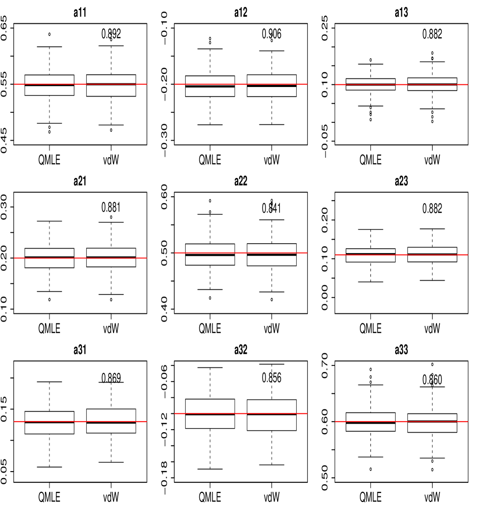
Figure 16: Boxplots of the QMLE and R-estimator (van der Waerden scores) under spherical Gaussian for $d=3$; sample size $n=1000$; $N=300$ replications. In each panel, the MSE ratio of the QMLE with respect to the R-estimator is reported. The horizontal red line represents the actual parameter value.

We also considered a trivariate ($d=3$) VAR(1), with parameter of interest $\mbox{\boldmath$\theta$}\in\mathbb{R}^{9}$, Gaussian and Gaussian mixture innovations, and sample size $n=1000$. The results, which confirm the bivariate ones, can be found in Appendix D.4 (Figures 15-16), along with details about the simulation design.

6 Real-data example

To conclude, we illustrate the applicability and good performance of our R-estimators in a real-data macroeconomic example. We consider the seasonally adjusted series of monthly housing starts (Hstarts) and the $30$-year conventional mortgage rate (Mortg—no need for seasonal adjustment) in the US from January 1989 to January 2016, with a sample size $n=325$ each (both series are freely available on the Federal Reserve Bank of Saint Louis website, to which we refer for details). The same time series were studied by Tsay (2014, Section 3.15.2). Following Tsay, we analyze the differenced series; Figure 3 displays plots of their demeaned differences. While the Mortg series seems to be driven by skew innovations (with large positive values more likely than the negative ones), the Hstarts series looks more symmetric about zero. Visual inspection suggests the presence of significant auto- and cross-correlations, as expected from macroeconomic theory.

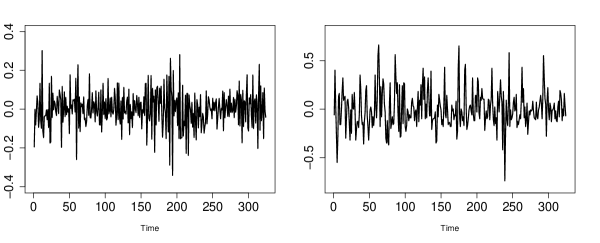
Figure 3: Plots of demeaned differences of the monthly housing starts (measured in thousands of units; left panel) and the $30$-year conventional mortgage rate (in percentage; right panel) in the US, from January 1989 through January 2016.

The AIC criterion selects a VARMA($3,1$) model, the parameters of which we estimated using the benchmark QMLE (see e.g. Tsay (2014), Chapter 3) and our R-estimators (sign, Spearman, and van der Waerden). The QMLE-based multivariate Ljung-Box test does not reject the model at nominal level 1%. We report the estimates (along with their standard error, SE, in parentheses) in Table 3 in the online Appendix E. Spotting the differences in Table 3 is all but simple, even though some look quite significant (see, for instance, the QMLE and R-estimates of ${\mbox{\boldmath$A$}}_{21}$ and ${\mbox{\boldmath$A$}}_{22}$) and analyzing them is even more difficult.

Impulse response functions (IRFs) are easier to read and interpret; they are widely applied in macroeconometrics—see e.g. Tsay (2014) for a book-length description. Intuitively the IRFs express the effect of changes in one variable on another variable in multivariate time series analysis. In the VARMA case, the IRF is obtained using a MA representation: see Tsay (2014, Section 3.15.2) and Appendix E.2 in the supplementary material for mathematical details. In Figures 4, we plot the estimated IRFs resulting from the QMLE and R-estimators. The top plots show the response of Hstarts to its own shocks (left panel) and to the shocks of Mortg; the bottom panels show the response of Mortg to its own shocks (right panel) and to the shocks of Hstarts. Looking at the plots, we see that all IRFs have similar patterns. For instance, for all estimators, the top left panel illustrates that the IRF of the Hstarts to its own shocks have two consecutive increases after two initial drops. However, the decay of the QMLE-based IRF is uniformly faster than the R-estimator-based ones. Also, the other plots exhibit a more pronounced decay in the QMLE-based IRFs. Thus, R-estimators suggest a more persistent impact of the shocks: decision makers should be aware of this inferential aspect in the implementation of their economic policy.

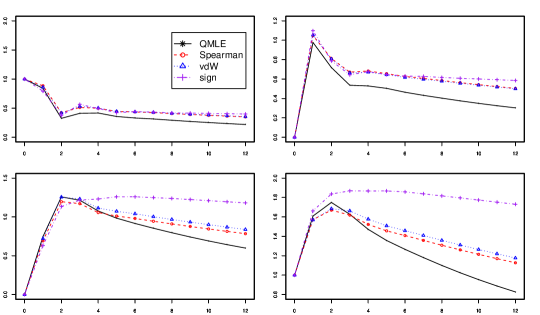
Figure 4: Plots of estimated impulse response functions of the VARMA($3,1$) model for the differenced Hstarts (top panels) and Mortg (bottom panels) data, based on the QMLE and the R-estimators.

7 Conclusions and perspectives

We define a class of R-estimators based on the novel concept of center-outward ranks and signs, itself closely related to the theory of optimal measure transportation. Monte Carlo experiments show that these estimators significantly outperform the classical QMLE under skew multivariate innovations, even when the validity conditions for the latter are satisfied. In a companion paper, we study the performance of the corresponding rank-based tests for VAR models, and, more particularly, propose a center-outward Durbin-Watson test for multiple-output regression and a test of VAR($p_{0}$) against VAR($p_{0}+1$) dependence. Our methodology is not limited to the VARMA case, though; its extension to nonlinear multivariate models, like the dynamic conditional correlation model of Engle (2002), is the subject of ongoing research.

Appendix A Technical material: algebraic preparation

Denote by ${\mbox{\boldmath$G$}}_{u}$ and ${\mbox{\boldmath$H$}}_{u}$, $u\in{\mathbb{Z}}$ the Green’s matrices associated with the linear difference operators ${\mbox{\boldmath$A$}}(L)$ and ${\mbox{\boldmath$B$}}(L)$ in Section 2.1: those matrices are defined as the solutions of the homogeneous linear recursions

$${\mbox{\boldmath$A$}}(L){\mbox{\boldmath$G$}}_{u}={\mbox{\boldmath$G$}}_{u}-\sum_{i=1}^{p}{\mbox{\boldmath$A$}}_{i}{\mbox{\boldmath$G$}}_{u-i}={\bf 0}\quad\text{and}\quad{\mbox{\boldmath$B$}}(L){\mbox{\boldmath$H$}}_{u}=\sum_{i=0}^{q}{\mbox{\boldmath$B$}}_{i}{\mbox{\boldmath$H$}}_{u-i}={\bf 0},\quad u\in\mathbb{Z}$$

with initial values ${\mbox{\boldmath$I$}}_{d},{\bf 0},\ldots,{\bf 0}$ at $u=0,-1,\ldots,-p+1$ and $u=0,-1,\ldots,-q+1$, respectively. Then, the residual process $\{{\mbox{\boldmath$Z$}}_{t}^{(n)}(\mbox{\boldmath$\theta$});1\leq t\leq n\}$ has the representation

$${\mbox{\boldmath$Z$}}_{t}^{(n)}(\mbox{\boldmath$\theta$})= \sum_{i=0}^{t-1}\sum_{j=0}^{p}{\mbox{\boldmath$H$}}_{i}{\mbox{\boldmath$A$}}_{j}{\mbox{\boldmath$X$}}^{(n)}_{t-i-j}$$

$$+\begin{bmatrix}{\mbox{\boldmath$H$}}_{t+q-1}&\cdots&{\mbox{\boldmath$H$}}_{t}\end{bmatrix}\begin{bmatrix}{\mbox{\boldmath$I$}}_{d}&{\mbox{\boldmath$0$}}&\cdots&{\mbox{\boldmath$0$}}\\ {\mbox{\boldmath$B$}}_{1}&{\mbox{\boldmath$I$}}_{d}&\cdots&{\mbox{\boldmath$0$}}\\ \vdots&\vdots&\ddots&\vdots\\ {\mbox{\boldmath$B$}}_{q-1}&{\mbox{\boldmath$B$}}_{q-2}&\cdots&{\mbox{\boldmath$I$}}_{d}\end{bmatrix}\begin{bmatrix}\mbox{\boldmath$\epsilon$}_{-q+1}\\ \vdots\\ \mbox{\boldmath$\epsilon$}_{0}\end{bmatrix}$$ (A.1)

(see Hallin (1986), Garel and Hallin (1995), or Hallin and Paindaveine (2004)).

Assumption (A1) ensures the exponential decrease of $\{\|{\mbox{\boldmath$H$}}_{u}\|,u\in{\mathbb{N}}\}$ as $u\to\infty$. Specifically, there exists some $\varepsilon>0$ such that $\|{\mbox{\boldmath$H$}}_{u}\|(1+\varepsilon)^{u}$ converges to $0$ as $u\rightarrow\infty$. This also holds for the Green matrices ${\mbox{\boldmath$G$}}_{u}$ associated with the operator ${\mbox{\boldmath$A$}}(L)$. It follows that the initial values $\{\mbox{\boldmath$\epsilon$}_{-q+1},\ldots,\mbox{\boldmath$\epsilon$}_{0}\}$ and $\{{\mbox{\boldmath$X$}}_{-p+1},\ldots,{\mbox{\boldmath$X$}}_{0}\}$ in (A.1), which are typically unobservable, have no asymptotic influence on the residuals nor any asymptotic results. Therefore, they all can safely be set to zero in the sequel. This allows us to invert the AR and MA polynomials, and to define the Green matrices ${\mbox{\boldmath$G$}}_{u}$ and ${\mbox{\boldmath$H$}}_{u}$ as the matrix coefficients of the inverted operators $({\mbox{\boldmath$A$}}(L))^{-1}$ and $({\mbox{\boldmath$B$}}(L))^{-1}$:

$$\sum_{u=0}^{\infty}{\mbox{\boldmath$G$}}_{u}z^{u}:=\left({\mbox{\boldmath$I$}}_{d}-\sum_{i=1}^{p}{\mbox{\boldmath$A$}}_{i}z^{i}\right)^{-1}\quad\text{and}\quad\sum_{u=0}^{\infty}{\mbox{\boldmath$H$}}_{u}z^{u}:=\left(\sum_{i=0}^{q}{\mbox{\boldmath$B$}}_{i}z^{i}\right)^{-1},\quad z\in{\mathbb{C}},|z|<1.$$

Associated with an arbitrary $d$-dimensional linear difference operator ${\mbox{\boldmath$C$}}(L):=\sum_{i=0}^{\infty}{\mbox{\boldmath$C$}}_{i}L^{i}$ (this of course includes operators of finite order $s$), define, for any integers $u$ and $v$, the $d^{2}u\times d^{2}v$ matrices

$${\mbox{\boldmath$C$}}_{u,v}^{(l)}:=\begin{bmatrix}{\mbox{\boldmath$C$}}_{0}\otimes{\mbox{\boldmath$I$}}_{d}&{\mbox{\boldmath$0$}}&\ldots&{\mbox{\boldmath$0$}}\\ {\mbox{\boldmath$C$}}_{1}\otimes{\mbox{\boldmath$I$}}_{d}&{\mbox{\boldmath$C$}}_{0}\otimes{\mbox{\boldmath$I$}}_{d}&\ldots&{\mbox{\boldmath$0$}}\\ \vdots&&\ddots&\vdots\\ {\mbox{\boldmath$C$}}_{v-1}\otimes{\mbox{\boldmath$I$}}_{d}&{\mbox{\boldmath$C$}}_{v-2}\otimes{\mbox{\boldmath$I$}}_{d}&\ldots&{\mbox{\boldmath$C$}}_{0}\otimes{\mbox{\boldmath$I$}}_{d}\\ \vdots&&&\vdots\\ {\mbox{\boldmath$C$}}_{u-1}\otimes{\mbox{\boldmath$I$}}_{d}&{\mbox{\boldmath$C$}}_{u-2}\otimes{\mbox{\boldmath$I$}}_{d}&\ldots&{\mbox{\boldmath$C$}}_{u-v}\otimes{\mbox{\boldmath$I$}}_{d}\end{bmatrix}$$

and

$${\mbox{\boldmath$C$}}_{u,v}^{(r)}:=\begin{bmatrix}{\mbox{\boldmath$I$}}_{d}\otimes{\mbox{\boldmath$C$}}_{0}&{\mbox{\boldmath$0$}}&\ldots&{\mbox{\boldmath$0$}}\\ {\mbox{\boldmath$I$}}_{d}\otimes{\mbox{\boldmath$C$}}_{1}&{\mbox{\boldmath$I$}}_{d}\otimes{\mbox{\boldmath$C$}}_{0}&\ldots&{\mbox{\boldmath$0$}}\\ \vdots&&\ddots&\vdots\\ {\mbox{\boldmath$I$}}_{d}\otimes{\mbox{\boldmath$C$}}_{v-1}&{\mbox{\boldmath$I$}}_{d}\otimes{\mbox{\boldmath$C$}}_{v-2}&\ldots&{\mbox{\boldmath$I$}}_{d}\otimes{\mbox{\boldmath$C$}}_{0}\\ \vdots&&&\vdots\\ {\mbox{\boldmath$I$}}_{d}\otimes{\mbox{\boldmath$C$}}_{u-1}&{\mbox{\boldmath$I$}}_{d}\otimes{\mbox{\boldmath$C$}}_{u-2}&\ldots&{\mbox{\boldmath$I$}}_{d}\otimes{\mbox{\boldmath$C$}}_{u-v}\end{bmatrix}.$$

Write ${\mbox{\boldmath$C$}}_{u}^{(l)}$ for ${\mbox{\boldmath$C$}}_{u,u}^{(l)}$ and ${\mbox{\boldmath$C$}}_{u}^{(r)}$ for ${\mbox{\boldmath$C$}}_{u,u}^{(r)}$. With this notation, note that ${\mbox{\boldmath$G$}}_{u}^{(l)},{\mbox{\boldmath$G$}}_{u}^{(r)},{\mbox{\boldmath$H$}}_{u}^{(l)}$, and ${\mbox{\boldmath$H$}}_{u}^{(r)}$ are the inverses of ${\mbox{\boldmath$A$}}_{u}^{(l)},{\mbox{\boldmath$A$}}_{u}^{(r)},{\mbox{\boldmath$B$}}_{u}^{(l)}$ and ${\mbox{\boldmath$B$}}_{u}^{(r)}$, respectively. Denoting by ${\mbox{\boldmath$C$}}_{u,v}^{\prime(l)}$ and ${\mbox{\boldmath$C$}}_{u,v}^{\prime(r)}$ the matrices associated with the transposed operator ${\mbox{\boldmath$C$}}^{\prime}(L):=\sum_{i=0}^{\infty}{\mbox{\boldmath$C$}}^{\prime}_{i}L^{i}$, we have ${\mbox{\boldmath$G$}}_{u}^{\prime(l)}\leavevmode\nobreak\ \!=\leavevmode\nobreak\ \!({\mbox{\boldmath$A$}}_{u}^{\prime(l)})^{-1}$, ${\mbox{\boldmath$H$}}_{u}^{\prime(l)}=({\mbox{\boldmath$B$}}_{u}^{\prime(l)})^{-1}$, and so on. Define the $d^{2}(p+q)\times d^{2}(p+q)$ matrix

$${\mbox{\boldmath$M$}}_{\mbox{\boldmath$\theta$}}:=({\mbox{\boldmath$G$}}^{\prime(l)}_{p+q,p}\vdots{\mbox{\boldmath$H$}}^{\prime(l)}_{p+q,q}):$$ (A.2)

under Assumption (A1), ${\mbox{\boldmath$M$}}_{\mbox{\boldmath$\theta$}}$ is of full rank.

Also, consider the operator ${\mbox{\boldmath$D$}}(L):={\mbox{\boldmath$I$}}_{d}+\sum_{i=1}^{p+q}{\mbox{\boldmath$D$}}_{i}L^{i}$ (note that ${\mbox{\boldmath$D$}}(L)$ and most quantities defined below depends on $\theta$; for simplicity, however, we are dropping this reference to $\theta$), where

$$\begin{bmatrix}{\mbox{\boldmath$D$}}_{1}^{\prime}\\ \vdots\\ {\mbox{\boldmath$D$}}_{p+q}^{\prime}\end{bmatrix}:=-\begin{bmatrix}{\mbox{\boldmath$G$}}_{q}&{\mbox{\boldmath$G$}}_{q-1}&\ldots&{\mbox{\boldmath$G$}}_{-p+1}\\ {\mbox{\boldmath$G$}}_{q+1}&{\mbox{\boldmath$G$}}_{q}&\ldots&{\mbox{\boldmath$G$}}_{-p+2}\\ \vdots&&\ddots&\vdots\\ {\mbox{\boldmath$G$}}_{p+q-1}&{\mbox{\boldmath$G$}}_{p+q-2}&\ldots&{\mbox{\boldmath$G$}}_{0}\\ {\mbox{\boldmath$H$}}_{p}&{\mbox{\boldmath$H$}}_{p-1}&\ldots&{\mbox{\boldmath$H$}}_{-q+1}\\ {\mbox{\boldmath$H$}}_{p+1}&{\mbox{\boldmath$H$}}_{p}&\ldots&{\mbox{\boldmath$H$}}_{-q+2}\\ \vdots&&\ddots&\vdots\\ {\mbox{\boldmath$H$}}_{p+q-1}&{\mbox{\boldmath$H$}}_{p+q-2}&\ldots&{\mbox{\boldmath$H$}}_{0}\end{bmatrix}^{-1}\begin{bmatrix}{\mbox{\boldmath$G$}}_{q+1}\\ \vdots\\ {\mbox{\boldmath$G$}}_{p+q}\\ {\mbox{\boldmath$H$}}_{p+1}\\ \vdots\\ {\mbox{\boldmath$H$}}_{p+q}\end{bmatrix}$$

(recall that ${\mbox{\boldmath$G$}}_{-1}={\mbox{\boldmath$G$}}_{-2}=\cdots={\mbox{\boldmath$G$}}_{-p+1}={\mbox{\boldmath$0$}}$ and ${\mbox{\boldmath$H$}}_{-1}={\mbox{\boldmath$H$}}_{-2}=\cdots={\mbox{\boldmath$H$}}_{-q+1}={\mbox{\boldmath$0$}}$). Let $\{\mbox{\boldmath$\psi$}_{t}^{(1)},\ldots,\mbox{\boldmath$\psi$}_{t}^{(p+q)}\}$ be a set of $d\times d$ matrices forming a fundamental system of solutions of the homogeneous linear difference equation associated with ${\mbox{\boldmath$D$}}(L)$. Such a system can be obtained from the Green matrices of the operator ${\mbox{\boldmath$D$}}(L)$ (see, e.g., Hallin 1986). Defining

$$\bar{\mbox{\boldmath$\psi$}}_{m}(\mbox{\boldmath$\theta$}):=\begin{bmatrix}\mbox{\boldmath$\psi$}_{1}^{(1)}&\ldots&\mbox{\boldmath$\psi$}_{1}^{(p+q)}\\ \mbox{\boldmath$\psi$}_{2}^{(1)}&\ldots&\mbox{\boldmath$\psi$}_{2}^{(p+q)}\\ \vdots&&\vdots\\ \mbox{\boldmath$\psi$}_{m}^{(1)}&\ldots&\mbox{\boldmath$\psi$}_{m}^{(p+q)}\end{bmatrix}\otimes{\mbox{\boldmath$I$}}_{d},$$

the Casorati matrix $\mathbf{C}_{\mbox{\boldmath$\psi$}}$ associated with ${\mbox{\boldmath$D$}}(L)$ is $\bar{\mbox{\boldmath$\psi$}}_{p+q}$. Finally, let

$${\mbox{\boldmath$P$}}_{\mbox{\boldmath$\theta$}}:=\mathbf{C}_{\mbox{\boldmath$\psi$}}^{-1}\quad\text{and}\quad{\mbox{\boldmath$Q$}}^{(n)}_{\mbox{\boldmath$\theta$}}:={\mbox{\boldmath$H$}}_{n-1}^{(r)}{\mbox{\boldmath$B$}}_{n-1}^{\prime(l)}\bar{\mbox{\boldmath$\psi$}}_{n-1}.$$ (A.3)

Appendix B Proofs

This appendix gathers the proofs of all mathematical results. Throughout, we consider $f\in{\cal F}_{d}$ (the family of densities introduced in Section 2) and assume that, for all $c\in{\mathbb{R}}^{+}$, there exist $b_{c;f}$ and $a_{c;f}$ in $\mathbb{R}$ such that $0<b_{c;f}\leq a_{c;f}<\infty$ and $b_{c;f}\leq f({\mbox{\boldmath$x$}})\leq a_{c;f}$ for $\|{\mbox{\boldmath$x$}}\|\leq c$.

Proof of Proposition 2.1.

The LAN result is essentially the same as in Garel and Hallin (1995, (LAN 2) in their Proposition 3.1) and, moving along the same lines as in the proof of Proposition 1 in Hallin and Paindaveine (2004), we obtain the form (2.3) of $\mbox{\boldmath$\Delta$}^{(n)}_{f}(\mbox{\boldmath$\theta$})$. The form of the asymptotic covariance matrix $\mbox{\boldmath$\Lambda$}_{f}(\mbox{\boldmath$\theta$})$ and its finiteness easily follow from applying Lemma 4.12 in Garel and Hallin (1995). Details are left to the reader. $\hfill\Box$

To prove Propositions 4.1 and 4.2, we first need to establish the asymptotic normality, under ${\rm P}^{(n)}_{\mbox{\boldmath$\theta$};f}$ and ${\rm P}^{(n)}_{\mbox{\boldmath$\theta$}+n^{-1/2}{\mbox{\boldmath$\tau$}};f}$, of the rank-based $\stackunder[1pt]{\mbox{\boldmath$\Delta$}}{\scriptscriptstyle\thicksim}^{(n)}_{{J}_{1},{J}_{2}}(\mbox{\boldmath$\theta$})$. As in the univariate case, due to the fact that the ranks are not mutually independent, the asymptotic normality of a rank statistic does not follow from classical central-limit theorems. The approach we are adopting here is inspired from Hájek, and consists in establishing an asymptotic representation result for the rank-based statistic under study—namely, its asymptotic equivalence with a sum of independent variable which are no longer rank-based—then proving the asymptotic normality of the latter. This is achieved here in a series of lemmas: Lemma B.1 deals with the asymptotic normality of $(n-i)^{1/2}\text{vec}(\bar{\mbox{\boldmath$\Gamma$}}_{i,{J}_{1},{J}_{2}}^{(n)}(\mbox{\boldmath$\theta$}))$, a corollary of which is the asymptotic normality of the truncated versions $\bar{\mbox{\boldmath$\Delta$}}^{(n)}_{m,{J}_{1},{J}_{2}}(\mbox{\boldmath$\theta$})$ of $\bar{\mbox{\boldmath$\Delta$}}^{(n)}_{{J}_{1},{J}_{2}}(\mbox{\boldmath$\theta$})$; Lemma B.3 provides the asymptotic representation of $\text{vec}(\stackunder[1pt]{\mbox{\boldmath$\Gamma$}}{\scriptscriptstyle\thicksim}_{i,{J}_{1},{J}_{2}}^{(n)}(\mbox{\boldmath$\theta$}))$ by $\text{vec}(\bar{\mbox{\boldmath$\Gamma$}}_{i,{J}_{1},{J}_{2}}^{(n)}(\mbox{\boldmath$\theta$}))$; the asymptotic representation of $\stackunder[1pt]{\mbox{\boldmath$\Delta$}}{\scriptscriptstyle\thicksim}^{(n)}_{{J}_{1},{J}_{2}}(\mbox{\boldmath$\theta$})$ by $\bar{\mbox{\boldmath$\Delta$}}^{(n)}_{{J}_{1},{J}_{2}}(\mbox{\boldmath$\theta$})$ and their asymptotic normality are obtained in Lemma B.4. The proofs of Propositions 4.1 and 4.2 follow.

Let us start with the asymptotic normality of $(n-i)^{1/2}\text{vec}(\bar{\mbox{\boldmath$\Gamma$}}_{i,{J}_{1},{J}_{2}}^{(n)}(\mbox{\boldmath$\theta$}))$.

Lemma B.1.

Let Assumptions (A1), (A2), and (A3) hold. Then, for any positive integer $i$, the vector $(n-i)^{1/2}\text{\rm vec}(\bar{\mbox{\boldmath$\Gamma$}}_{i,{J}_{1},{J}_{2}}^{(n)}(\mbox{\boldmath$\theta$}))$ in (4.7) is asymptotically normal with mean $\mathrm{𝟎}$ under ${\rm P}^{(n)}_{\mbox{\boldmath$\theta$};f}$, mean ${\mbox{\boldmath$K$}}_{{J}_{1},{J}_{2},{f}}{\mbox{\boldmath$Q$}}_{i,\mbox{\boldmath$\theta$}}{\mbox{\boldmath$P$}}_{\mbox{\boldmath$\theta$}}{\mbox{\boldmath$M$}}_{\mbox{\boldmath$\theta$}}{\mbox{\boldmath$\tau$}}$ under ${\rm P}^{(n)}_{\mbox{\boldmath$\theta$}+n^{-1/2}{\mbox{\boldmath$\tau$}};f}$, and covariance $d^{-2}\sigma^{2}_{{J}_{1}}\sigma^{2}_{{J}_{2}}{\mbox{\boldmath$I$}}_{d^{2}}$ under both.

Proof.

Since $L^{(n)}_{\mbox{\boldmath$\theta$}+n^{-1/2}{\mbox{\boldmath$\tau$}}/\mbox{\boldmath$\theta$};{f}}={\mbox{\boldmath$\tau$}}^{\prime}\mbox{\boldmath$\Delta$}^{(n)}_{f}(\mbox{\boldmath$\theta$})-\frac{1}{2}{\mbox{\boldmath$\tau$}}^{\prime}\mbox{\boldmath$\Lambda$}_{f}(\mbox{\boldmath$\theta$}){\mbox{\boldmath$\tau$}}+o_{\rm P}(1)$, the joint asymptotic normality of $(n-i)^{1/2}\text{\rm vec}(\bar{\mbox{\boldmath$\Gamma$}}_{i,{J}_{1},{J}_{2}}^{(n)}(\mbox{\boldmath$\theta$}))$ and $L^{(n)}_{\mbox{\boldmath$\theta$}+n^{-1/2}{\mbox{\boldmath$\tau$}}/\mbox{\boldmath$\theta$};{f}}$ under ${\rm P}^{(n)}_{\mbox{\boldmath$\theta$};f}$ follows, via the classical Wold-Cramér argument, from the asymptotic normality of

$$N^{(n)}_{{\boldsymbol{\alpha}},\beta}:=(n-i)^{1/2}{\boldsymbol{\alpha}}^{\prime}\text{\rm vec}(\bar{\mbox{\boldmath$\Gamma$}}_{i,{J}_{1},{J}_{2}}^{(n)}(\mbox{\boldmath$\theta$}))+\beta{\mbox{\boldmath$\tau$}}^{\prime}\mbox{\boldmath$\Delta$}^{(n)}_{f}(\mbox{\boldmath$\theta$})$$

for arbitrary ${\boldsymbol{\alpha}}\in\mathbb{R}^{d^{2}}$ and $\beta\in\mathbb{R}$. Since ${\mbox{\boldmath$Z$}}_{1}^{(n)},\ldots,{\mbox{\boldmath$Z$}}_{n}^{(n)}$ are i.i.d. and ${\mbox{\boldmath$F$}}_{{\mspace{-1.0mu}{\scriptscriptstyle\pm}},t}:={\mbox{\boldmath$F$}}_{\mspace{-1.0mu}{\scriptscriptstyle\pm}}({\mbox{\boldmath$Z$}}^{(n)}_{t})$ is uniform over the unit ball, ${N}^{(n)}_{{\boldsymbol{\alpha}},\beta}$ is a sum of martingale differences. If it is uniformly square-integrable, with finite variance $C^{(n)}_{{\boldsymbol{\alpha}},\beta}$, say, such that $\lim_{n\to\infty}C^{(n)}_{{\boldsymbol{\alpha}},\beta}=:C_{{\boldsymbol{\alpha}},\beta}$ exists and is finite, the martingale central limit theorem applies, and $N^{(n)}_{{\boldsymbol{\alpha}},\beta}$ is asymptotically normal with mean $0$ and variance $C_{{\boldsymbol{\alpha}},\beta}$. Now, the variance of ${N}^{(n)}_{{\boldsymbol{\alpha}},\beta}$ takes the form

$$C^{(n)}_{{\boldsymbol{\alpha}},\beta} =(n-i){\boldsymbol{\alpha}}^{\prime}{\mathrm{Var}}\big{(}\text{\rm vec}(\bar{\mbox{\boldmath$\Gamma$}}_{i,{J}_{1},{J}_{2}}^{(n)}(\mbox{\boldmath$\theta$}))\big{)}{\boldsymbol{\alpha}}$$

$$\qquad+2\beta{\boldsymbol{\alpha}}^{\prime}(n-i)^{1/2}{\mathrm{Cov}}\big{(}\text{\rm vec}(\bar{\mbox{\boldmath$\Gamma$}}_{i,{J}_{1},{J}_{2}}^{(n)}(\mbox{\boldmath$\theta$})),{\mbox{\boldmath$\tau$}}^{\prime}\mbox{\boldmath$\Delta$}^{(n)}_{f}(\mbox{\boldmath$\theta$})\big{)}$$

$$\qquad+\beta^{2}{\mbox{\boldmath$\tau$}}^{\prime}{\mathrm{Var}}\big{(}\mbox{\boldmath$\Delta$}^{(n)}_{f}(\mbox{\boldmath$\theta$})\big{)}{\mbox{\boldmath$\tau$}}.$$

The entries of each $\bar{\mbox{\boldmath$\Gamma$}}_{i,{J}_{1},{J}_{2}}^{(n)}(\mbox{\boldmath$\theta$})$ are uniformly square-integrable. As for $\mbox{\boldmath$\Delta$}^{(n)}_{f}(\mbox{\boldmath$\theta$})$, it follows from Lemma 2.2 in Hallin and Werker (2003) that, for any LAN family, a uniformly $p$th-order integrable version of the central sequence exists: without loss of generality, let us assume that $\mbox{\boldmath$\Delta$}^{(n)}_{f}(\mbox{\boldmath$\theta$})$, for $p=2$, is one of them. The sequence ${N}^{(n)}_{{\boldsymbol{\alpha}},\beta}$ thus has a limiting ${\cal N}(0,C_{{\boldsymbol{\alpha}},\beta})$ distribution provided that $\lim_{n\to\infty}C^{(n)}_{{\boldsymbol{\alpha}},\beta}=:C_{{\boldsymbol{\alpha}},\beta}$ exists and is finite.

Due to the independence between the signs ${\mbox{\boldmath$S$}}_{{\mspace{-1.0mu}{\scriptscriptstyle\pm}},t}:={\mbox{\boldmath$F$}}_{{\mspace{-1.0mu}{\scriptscriptstyle\pm}},t}/\|{\mbox{\boldmath$F$}}_{{\mspace{-1.0mu}{\scriptscriptstyle\pm}},t}\|$ and the moduli $\|{\mbox{\boldmath$F$}}_{{\mspace{-1.0mu}{\scriptscriptstyle\pm}},t}\|$ (which follows from the fact that ${\mbox{\boldmath$F$}}_{{\mspace{-1.0mu}{\scriptscriptstyle\pm}},t}\sim{\mathrm{U}}_{d}$), and due to the fact that ${\mbox{\boldmath$Z$}}_{1}^{(n)},\ldots,{\mbox{\boldmath$Z$}}_{n}^{(n)}$ are i.i.d.,

$$\lim_{n\to\infty}{\mathrm{Var}}\big{(}\text{\rm vec}(\bar{\mbox{\boldmath$\Gamma$}}_{i,{J}_{1},{J}_{2}}^{(n)}(\mbox{\boldmath$\theta$}))\big{)}= \lim_{n\to\infty}\mathrm{E}\left\{(n-i)\text{vec}\bar{\mbox{\boldmath$\Gamma$}}_{i,{J}_{1},{J}_{2}}^{(n)}(\mbox{\boldmath$\theta$})(\text{vec}\bar{\mbox{\boldmath$\Gamma$}}_{i,{J}_{1},{J}_{2}}^{(n)}(\mbox{\boldmath$\theta$}))^{\prime}\right\}$$

$$= \lim_{n\to\infty}(n-i)^{-1}\mathrm{E}\left\{\left[\sum_{t=i+1}^{n}{J}_{1}(\|{\mbox{\boldmath$F$}}_{{\mspace{-1.0mu}{\scriptscriptstyle\pm}},t}\|){J}_{2}(\|{\mbox{\boldmath$F$}}_{{\mspace{-1.0mu}{\scriptscriptstyle\pm}},t-i}\|)\text{vec}({\mbox{\boldmath$S$}}_{{\mspace{-1.0mu}{\scriptscriptstyle\pm}},t}{\mbox{\boldmath$S$}}^{\prime}_{{\mspace{-1.0mu}{\scriptscriptstyle\pm}},t-i})\right]\right.$$

$$\qquad\qquad\qquad\times\left.\left[\sum_{t=i+1}^{n}{J}_{1}(\|{\mbox{\boldmath$F$}}_{{\mspace{-1.0mu}{\scriptscriptstyle\pm}},t}\|){J}_{2}(\|{\mbox{\boldmath$F$}}_{{\mspace{-1.0mu}{\scriptscriptstyle\pm}},t-i}\|)\text{vec}({\mbox{\boldmath$S$}}_{{\mspace{-1.0mu}{\scriptscriptstyle\pm}},t}{\mbox{\boldmath$S$}}^{\prime}_{{\mspace{-1.0mu}{\scriptscriptstyle\pm}},t-i})\right]^{\prime}\right\}$$

$$= \frac{1}{d^{2}}\sigma^{2}_{{J}_{1}}\sigma^{2}_{{J}_{2}}{\mbox{\boldmath$I$}}_{d^{2}},$$ (B.1)

where the last equation follows from the uniform distribution of ${\mbox{\boldmath$S$}}_{{\mspace{-1.0mu}{\scriptscriptstyle\pm}},t}$ over $\mathcal{S}_{d-1}$. Next, the uniform square-integrability of $\mbox{\boldmath$\Delta$}^{(n)}_{f}(\mbox{\boldmath$\theta$})$ and its asymptotic normality in Proposition 2.1 yield

$$\underset{n\rightarrow\infty}{\lim}(n-i)^{1/2}{\mathrm{Cov}}\big{(}\text{\rm vec}(\bar{\mbox{\boldmath$\Gamma$}}_{i,{J}_{1},{J}_{2}}^{(n)}(\mbox{\boldmath$\theta$})),{\mbox{\boldmath$\tau$}}^{\prime}\mbox{\boldmath$\Delta$}^{(n)}_{f}(\mbox{\boldmath$\theta$})\big{)}$$

$$=\underset{n\rightarrow\infty}{\lim}{\mathrm{E}}\left[(n-i)^{1/2}\text{vec}(\bar{\mbox{\boldmath$\Gamma$}}_{i,{J}_{1},{J}_{2}}^{(n)}(\mbox{\boldmath$\theta$})){\mbox{\boldmath$\tau$}}^{\prime}\mbox{\boldmath$\Delta$}^{(n)}_{f}(\mbox{\boldmath$\theta$})\right]$$

$$=\underset{n\rightarrow\infty}{\lim}{\mathrm{E}}\left[(n-i)^{1/2}\text{vec}(\bar{\mbox{\boldmath$\Gamma$}}_{i,{J}_{1},{J}_{2}}^{(n)}(\mbox{\boldmath$\theta$}))\mbox{\boldmath$\Gamma$}_{f}^{(n)\prime}(\mbox{\boldmath$\theta$})\right]{\mbox{\boldmath$Q$}}_{\mbox{\boldmath$\theta$}}^{(n)}{\mbox{\boldmath$P$}}_{\mbox{\boldmath$\theta$}}{\mbox{\boldmath$M$}}_{\mbox{\boldmath$\theta$}}{\mbox{\boldmath$\tau$}},$$ (B.2)

where the last equality follows from (2.3). Due to the independence of ${\mbox{\boldmath$Z$}}_{i}^{(n)}$ and ${\mbox{\boldmath$Z$}}_{j}^{(n)}$ for $i\neq j$, only $\mbox{\boldmath$\Gamma$}_{i,f}^{(n)}(\mbox{\boldmath$\theta$})$ in $\mbox{\boldmath$\Gamma$}_{f}^{(n)}(\mbox{\boldmath$\theta$})$ is contributing to (B.2). Therefore, using the block matrix form of ${\mbox{\boldmath$Q$}}^{(n)}_{\mbox{\boldmath$\theta$}}=\big{(}{\mbox{\boldmath$Q$}}_{1,\mbox{\boldmath$\theta$}}^{\prime}\ldots{\mbox{\boldmath$Q$}}_{n-1,\mbox{\boldmath$\theta$}}^{\prime}\big{)}^{\prime}$, the expression in (B.2) reduces to

$$\underset{n\rightarrow\infty}{\lim}(n-i){\mathrm{E}}\left[\text{vec}(\bar{\mbox{\boldmath$\Gamma$}}_{i,{J}_{1},{J}_{2}}^{(n)}(\mbox{\boldmath$\theta$}))(\text{vec}(\mbox{\boldmath$\Gamma$}_{i,{f}}^{(n)}(\mbox{\boldmath$\theta$})))^{\prime}\right]{\mbox{\boldmath$Q$}}_{i,\mbox{\boldmath$\theta$}}{\mbox{\boldmath$P$}}_{\mbox{\boldmath$\theta$}}{\mbox{\boldmath$M$}}_{\mbox{\boldmath$\theta$}}{\mbox{\boldmath$\tau$}}.$$ (B.3)

From (2.5), we have

$$(n-i){\mathrm{E}}\left[\text{vec}(\bar{\mbox{\boldmath$\Gamma$}}_{i,{J}_{1},{J}_{2}}^{(n)}(\mbox{\boldmath$\theta$}))(\text{vec}(\mbox{\boldmath$\Gamma$}_{i,{f}}^{(n)}(\mbox{\boldmath$\theta$})))^{\prime}\right]$$

$$\quad=(n-i)^{-1}{\mathrm{E}}\left\{\left[\sum_{t=i+1}^{n}{J}_{1}(\|{\mbox{\boldmath$F$}}_{{\mspace{-1.0mu}{\scriptscriptstyle\pm}},t}\|){J}_{2}(\|{\mbox{\boldmath$F$}}_{{\mspace{-1.0mu}{\scriptscriptstyle\pm}},t-i}\|)\text{vec}({\mbox{\boldmath$S$}}_{{\mspace{-1.0mu}{\scriptscriptstyle\pm}},t}{\mbox{\boldmath$S$}}^{\prime}_{{\mspace{-1.0mu}{\scriptscriptstyle\pm}},t-i})\right]\left[\sum_{t=i+1}^{n}\text{vec}(\mbox{\boldmath$\varphi$}_{f}({\mbox{\boldmath$Z$}}_{t}^{(n)})){\mbox{\boldmath$Z$}}^{\prime}_{t-i})\right]^{\prime}\right\}$$

$$\quad={\mathrm{E}}\big{[}{J}_{1}(\|{\mbox{\boldmath$F$}}_{{\mspace{-1.0mu}{\scriptscriptstyle\pm}},t}\|){J}_{2}(\|{\mbox{\boldmath$F$}}_{{\mspace{-1.0mu}{\scriptscriptstyle\pm}},t-i}\|)({\mbox{\boldmath$I$}}_{d}\otimes{\mbox{\boldmath$S$}}_{{\mspace{-1.0mu}{\scriptscriptstyle\pm}},t}){\mbox{\boldmath$S$}}_{{\mspace{-1.0mu}{\scriptscriptstyle\pm}},t-i}{\mbox{\boldmath$Z$}}^{\prime}_{t-i}({\mbox{\boldmath$I$}}_{d}\otimes\mbox{\boldmath$\varphi$}^{\prime}_{f}({\mbox{\boldmath$Z$}}_{t}^{(n)}))\big{]}\quad$$ (B.4)

where the last two equalities follow from the independence of ${\mbox{\boldmath$Z$}}_{1}^{(n)},\ldots,{\mbox{\boldmath$Z$}}_{n}^{(n)}$ and the uniform distribution of ${\mbox{\boldmath$F$}}_{{\mspace{-1.0mu}{\scriptscriptstyle\pm}},t}\sim{\mathrm{U}}_{d}$. In view of (2.6), (B.2), (B.3) and (B.4), we thus obtain

$$\underset{n\rightarrow\infty}{\lim}(n-i)^{1/2}{\mathrm{Cov}}\big{(}\text{\rm vec}(\bar{\mbox{\boldmath$\Gamma$}}_{i,{J}_{1},{J}_{2}}^{(n)}(\mbox{\boldmath$\theta$})),{\mbox{\boldmath$\tau$}}^{\prime}\mbox{\boldmath$\Delta$}^{(n)}_{f}(\mbox{\boldmath$\theta$})\big{)}={\mbox{\boldmath$K$}}_{{J}_{1},{J}_{2},{f}}{\mbox{\boldmath$Q$}}_{i,\mbox{\boldmath$\theta$}}{\mbox{\boldmath$P$}}_{\mbox{\boldmath$\theta$}}{\mbox{\boldmath$M$}}_{\mbox{\boldmath$\theta$}}{\mbox{\boldmath$\tau$}}.$$ (B.5)

Combining (B.1), (B.5) and the asymptotic normality of $\mbox{\boldmath$\Delta$}^{(n)}_{f}(\mbox{\boldmath$\theta$})$ in Proposition 2.1 yields, for arbitrary ${\boldsymbol{\alpha}}$ and $\beta$,

$$\underset{n\rightarrow\infty}{\lim}C^{(n)}_{{\boldsymbol{\alpha}},\beta}={\boldsymbol{\alpha}}^{\prime}{\boldsymbol{\alpha}}d^{-2}\sigma^{2}_{{J}_{1}}\sigma^{2}_{{J}_{2}}+2\beta{\boldsymbol{\alpha}}^{\prime}{\mbox{\boldmath$K$}}_{{J}_{1},{J}_{2},{f}}{\mbox{\boldmath$Q$}}_{i,\mbox{\boldmath$\theta$}}{\mbox{\boldmath$P$}}_{\mbox{\boldmath$\theta$}}{\mbox{\boldmath$M$}}_{\mbox{\boldmath$\theta$}}{\mbox{\boldmath$\tau$}}+\beta^{2}{\mbox{\boldmath$\tau$}}^{\prime}\mbox{\boldmath$\Lambda$}_{f}(\mbox{\boldmath$\theta$}){\mbox{\boldmath$\tau$}}.$$ (B.6)

It follows that $\big{(}(n-i)^{1/2}\text{vec}^{\prime}(\bar{\mbox{\boldmath$\Gamma$}}_{i,{J}_{1},{J}_{2}}^{(n)}(\mbox{\boldmath$\theta$})),\ L^{(n)}_{\mbox{\boldmath$\theta$}+n^{-1/2}{\mbox{\boldmath$\tau$}}/\mbox{\boldmath$\theta$};{f}}\big{)}^{\prime}$, under ${\rm P}^{(n)}_{\mbox{\boldmath$\theta$};f}$, is asymptotically jointly normal, with mean $\left({\mathbf{0}}^{\prime},-\frac{1}{2}{\mbox{\boldmath$\tau$}}^{\prime}\mbox{\boldmath$\Lambda$}_{f}(\mbox{\boldmath$\theta$}){\mbox{\boldmath$\tau$}}\right)^{\prime}$ and covariance

$$\begin{bmatrix}d^{-2}\sigma^{2}_{{J}_{1}}\sigma^{2}_{{J}_{2}}{\mbox{\boldmath$I$}}_{d^{2}}&{\mbox{\boldmath$K$}}_{{J}_{1},{J}_{2},{f}}{\mbox{\boldmath$Q$}}_{i,\mbox{\boldmath$\theta$}}{\mbox{\boldmath$P$}}_{\mbox{\boldmath$\theta$}}{\mbox{\boldmath$M$}}_{\mbox{\boldmath$\theta$}}{\mbox{\boldmath$\tau$}}\\ ({\mbox{\boldmath$K$}}_{{J}_{1},{J}_{2},{f}}{\mbox{\boldmath$Q$}}_{i,\mbox{\boldmath$\theta$}}{\mbox{\boldmath$P$}}_{\mbox{\boldmath$\theta$}}{\mbox{\boldmath$M$}}_{\mbox{\boldmath$\theta$}}{\mbox{\boldmath$\tau$}})^{\prime}&{\mbox{\boldmath$\tau$}}^{\prime}\mbox{\boldmath$\Lambda$}_{f}(\mbox{\boldmath$\theta$}){\mbox{\boldmath$\tau$}}\end{bmatrix}.$$ (B.7)

The desired result then readily follows from applying Le Cam’s third Lemma.∎

Recall that ${\mbox{\boldmath$T$}}^{(n)}_{\mbox{\boldmath$\theta$}}={\mbox{\boldmath$M$}}_{\mbox{\boldmath$\theta$}}^{\prime}{\mbox{\boldmath$P$}}_{\mbox{\boldmath$\theta$}}^{\prime}{\mbox{\boldmath$Q$}}_{\mbox{\boldmath$\theta$}}^{(n)\prime}$. For any positive integer $m\leq n-1$, let

$$\bar{\mbox{\boldmath$\Delta$}}^{(n)}_{m,{J}_{1},{J}_{2}}(\mbox{\boldmath$\theta$}):={\mbox{\boldmath$T$}}^{(m+1)}_{\mbox{\boldmath$\theta$}}\bar{\mbox{\boldmath$\Gamma$}}_{{J}_{1},{J}_{2}}^{(m,n)}(\mbox{\boldmath$\theta$}),$$ (B.8)

where

$$\bar{\mbox{\boldmath$\Gamma$}}_{{J}_{1},{J}_{2}}^{(m,n)}(\mbox{\boldmath$\theta$}):=\big{(}(n-1)^{1/2}(\text{vec}\bar{\mbox{\boldmath$\Gamma$}}_{1,{J}_{1},{J}_{2}}^{(n)}(\mbox{\boldmath$\theta$}))^{\prime},\ldots,(n-m)^{1/2}(\text{vec}\bar{\mbox{\boldmath$\Gamma$}}_{m,{J}_{1},{J}_{2}}^{(n)}(\mbox{\boldmath$\theta$})\big{)}^{\prime})^{\prime}:$$

clearly, $\bar{\mbox{\boldmath$\Delta$}}^{(n)}_{m,{J}_{1},{J}_{2}}(\mbox{\boldmath$\theta$})$, it is the truncated version of $\bar{\mbox{\boldmath$\Delta$}}^{(n)}_{{J}_{1},{J}_{2}}(\mbox{\boldmath$\theta$})$ defined in Section 4.1. The asymptotic normality of $\bar{\mbox{\boldmath$\Delta$}}^{(n)}_{m,{J}_{1},{J}_{2}}(\mbox{\boldmath$\theta$})$ follows from Lemma B.1 as a corollary.

Corollary B.1.

Let Assumptions (A1), (A2), and (A3) hold. Then, for any positive integer $m$, the vector $\bar{\mbox{\boldmath$\Delta$}}^{(n)}_{m,{J}_{1},{J}_{2}}(\mbox{\boldmath$\theta$})$ in (B.8) is asymptotically normal, with mean $\mathrm{𝟎}$ under ${\rm P}^{(n)}_{\mbox{\boldmath$\theta$};f}$, mean

$${\mbox{\boldmath$T$}}^{(m+1)}_{\mbox{\boldmath$\theta$}}({\mbox{\boldmath$I$}}_{m}\otimes{\mbox{\boldmath$K$}}_{{J}_{1},{J}_{2},f}){\mbox{\boldmath$T$}}^{(m+1)^{\prime}}_{\mbox{\boldmath$\theta$}}{\mbox{\boldmath$\tau$}}$$ (B.9)

under ${\rm P}^{(n)}_{\mbox{\boldmath$\theta$}+n^{-1/2}{\mbox{\boldmath$\tau$}};f}$, and covariance $d^{-2}\sigma^{2}_{{J}_{1}}\sigma^{2}_{{J}_{2}}{\mbox{\boldmath$T$}}^{(m+1)}_{\mbox{\boldmath$\theta$}}{\mbox{\boldmath$T$}}^{(m+1)^{\prime}}_{\mbox{\boldmath$\theta$}}$ under both.

The following auxiliary lemma, which follows along the same lines as Lemma 4 in Hallin and Paindaveine (2002) and Lemma 5 in Hallin and Paindaveine (2004), will be useful in subsequent proofs.

Lemma B.2.

Let $i\in\{1,\ldots,n-1\}$ and $t,{t^{\prime}}\in\{i+1,\ldots,n\}$ be such that $t\neq{t^{\prime}}$. Assume that $g:{\mathbb{R}}^{nd}={\mathbb{R}}^{d}\times\cdots\times{\mathbb{R}}^{d}\rightarrow{\mathbb{R}}$ is even in all its arguments, and such that the expectation in (B.10) below exists. Then, under ${\rm P}^{(n)}_{\mbox{\boldmath$\theta$};f}$,

$${\mathrm{E}}\big{[}g({\mbox{\boldmath$Z$}}_{1}^{(n)},\ldots,{\mbox{\boldmath$Z$}}_{n}^{(n)})({\mbox{\boldmath$P$}}_{t}^{\prime}{\mbox{\boldmath$Q$}}_{t})({\mbox{\boldmath$R$}}_{t-i}^{\prime}{\mbox{\boldmath$S$}}_{t^{\prime}-i})\big{]}=0,$$ (B.10)

where ${\mbox{\boldmath$P$}}_{t},{\mbox{\boldmath$Q$}}_{t},{\mbox{\boldmath$R$}}_{t}$ and ${\mbox{\boldmath$S$}}_{t}$ are any four random vectors among ${\mbox{\boldmath$S$}}^{(n)}_{{\mspace{-1.0mu}{\scriptscriptstyle\pm}},t}$ and ${\mbox{\boldmath$S$}}^{(n)}_{{\mspace{-1.0mu}{\scriptscriptstyle\pm}},t}-{\mbox{\boldmath$S$}}_{{\mspace{-1.0mu}{\scriptscriptstyle\pm}},t}$.

The next lemma establishes an asymptotic representation result for the rank-based cross-covariance matrices $\stackunder[1pt]{\mbox{\boldmath$\Gamma$}}{\scriptscriptstyle\thicksim}_{i,{J}_{1},{J}_{2}}^{(n)}(\mbox{\boldmath$\theta$})$ defined in (3.11) by showing their asymptotic equivalence with $\bar{\mbox{\boldmath$\Gamma$}}_{i,{J}_{1},{J}_{2}}^{(n)}(\mbox{\boldmath$\theta$})$ defined in (4.7). LAN implies that ${\rm P}^{(n)}_{\mbox{\boldmath$\theta$}+n^{-1/2}{\mbox{\boldmath$\tau$}};f}$ and ${\rm P}^{(n)}_{\mbox{\boldmath$\theta$};f}$ are mutually contiguous; (B.11) therefore holds under both. This asymptotic representation in the Hájek style of a center-outward serial rank statistic extends to a multivariate setting a univariate result first established by Hallin et al. (1985).

Lemma B.3.

Let Assumptions (A1), (A2), and (A3) hold. Then, for any positive integer $i$,

$$\text{\rm vec}\left(\stackunder[1pt]{\mbox{\boldmath$\Gamma$}}{\scriptscriptstyle\thicksim}_{i,{J}_{1},{J}_{2}}^{(n)}(\mbox{\boldmath$\theta$})-\bar{\mbox{\boldmath$\Gamma$}}_{i,{J}_{1},{J}_{2}}^{(n)}(\mbox{\boldmath$\theta$})\right)=o_{\rm P}(n^{-1/2})$$ (B.11)

under ${\rm P}^{(n)}_{\mbox{\boldmath$\theta$};f}$ and ${\rm P}^{(n)}_{\mbox{\boldmath$\theta$}+n^{-1/2}{\mbox{\boldmath$\tau$}};f}$, as $n\rightarrow\infty$.

Proof.

Note that $(n-i)^{1/2}(\stackunder[1pt]{\mbox{\boldmath$\Gamma$}}{\scriptscriptstyle\thicksim}_{i,{J}_{1},{J}_{2}}^{(n)}(\mbox{\boldmath$\theta$})-\bar{\mbox{\boldmath$\Gamma$}}_{i,{J}_{1},{J}_{2}}^{(n)}(\mbox{\boldmath$\theta$}))=(n-i)^{-1/2}({\boldsymbol{\delta}}_{1}^{(n)}+{\boldsymbol{\delta}}_{2}^{(n)})$ where

$${\boldsymbol{\delta}}_{1}^{(n)}:=(n-i)^{-1/2}\sum_{t=i+1}^{n}\left({J}_{1}(\frac{R^{(n)}_{{\mspace{-1.0mu}{\scriptscriptstyle\pm}},t}}{n_{R}+1}){J}_{2}(\frac{R^{(n)}_{{\mspace{-1.0mu}{\scriptscriptstyle\pm}},t-i}}{n_{R}+1})-{J}_{1}(\|{\mbox{\boldmath$F$}}_{{\mspace{-1.0mu}{\scriptscriptstyle\pm}},t}\|){J}_{2}(\|{\mbox{\boldmath$F$}}_{{\mspace{-1.0mu}{\scriptscriptstyle\pm}},t-i}\|)\right){\mbox{\boldmath$S$}}^{(n)}_{{\mspace{-1.0mu}{\scriptscriptstyle\pm}},t}{\mbox{\boldmath$S$}}^{(n)\prime}_{{\mspace{-1.0mu}{\scriptscriptstyle\pm}},t-i}$$

and

$${\boldsymbol{\delta}}_{2}^{(n)}:=(n-i)^{-1/2}\sum_{t=i+1}^{n}{J}_{1}(\|{\mbox{\boldmath$F$}}_{{\mspace{-1.0mu}{\scriptscriptstyle\pm}},t}\|){J}_{2}(\|{\mbox{\boldmath$F$}}_{{\mspace{-1.0mu}{\scriptscriptstyle\pm}},t-i}\|)\left({\mbox{\boldmath$S$}}^{(n)}_{{\mspace{-1.0mu}{\scriptscriptstyle\pm}},t}{\mbox{\boldmath$S$}}^{(n)\prime}_{{\mspace{-1.0mu}{\scriptscriptstyle\pm}},t-i}-{\mbox{\boldmath$S$}}_{{\mspace{-1.0mu}{\scriptscriptstyle\pm}},t}{\mbox{\boldmath$S$}}^{\prime}_{{\mspace{-1.0mu}{\scriptscriptstyle\pm}},t-i}\right).$$

It suffices to show that $\text{vec}({\boldsymbol{\delta}}_{1}^{(n)})$ and $\text{vec}({\boldsymbol{\delta}}_{2}^{(n)})$ both converge in quadratic mean to zero as $n\rightarrow\infty$ under ${\rm P}^{(n)}_{\mbox{\boldmath$\theta$};f}$.

Let $\|\cdot\|_{L^{2}}$ denote the $l_{2}$-norm. For ${\boldsymbol{\delta}}_{1}^{(n)}$, we make use of Lemma B.2, and we exploit the independence of the ranks $\{R^{(n)}_{{\mspace{-1.0mu}{\scriptscriptstyle\pm}},t};t=1,\ldots,n\}$ and the signs $\{{\mbox{\boldmath$S$}}^{(n)}_{{\mspace{-1.0mu}{\scriptscriptstyle\pm}},t};t=1,\ldots,n\}$ (see Hallin (2017)). Given that $(\text{vec}{\mbox{\boldmath$A$}})^{\prime}(\text{vec}{\mbox{\boldmath$B$}})=\text{tr}({\mbox{\boldmath$A$}}^{\prime}{\mbox{\boldmath$B$}})$, we have

$$\big{\|}\text{vec}({\boldsymbol{\delta}}_{1}^{(n)})\big{\|}_{L^{2}}^{2}=(n-i)^{-1}\sum_{t=i+1}^{n}{\mathrm{E}}\left[\left({J}_{1}(\frac{R^{(n)}_{{\mspace{-1.0mu}{\scriptscriptstyle\pm}},t}}{n_{R}+1}){J}_{2}(\frac{R^{(n)}_{{\mspace{-1.0mu}{\scriptscriptstyle\pm}},t-i}}{n_{R}+1})-{J}_{1}(\|{\mbox{\boldmath$F$}}_{{\mspace{-1.0mu}{\scriptscriptstyle\pm}},t}\|){J}_{2}(\|{\mbox{\boldmath$F$}}_{{\mspace{-1.0mu}{\scriptscriptstyle\pm}},t-i}\|)\right)^{2}\right].$$

The Glivenko-Cantelli result in Hallin (2017, Proposition 5.1) entails

$${\max}_{1\leq t\leq n}\Big{|}R^{(n)}_{{\mspace{-1.0mu}{\scriptscriptstyle\pm}},t}/(n_{R}+1)-\|{\mbox{\boldmath$F$}}_{{\mspace{-1.0mu}{\scriptscriptstyle\pm}},t}\|\Big{|}\rightarrow 0\quad a.s.\quad\text{as}\quad n\rightarrow\infty.$$ (B.12)

In view of the assumptions made on ${J}_{1}$ and ${J}_{2}$, Lemma 6.1.6.1 of Hájek et al. (1999) yields

$$\|\text{vec}({\boldsymbol{\delta}}_{1}^{(n)})\|_{L^{2}}^{2}\rightarrow 0\quad\text{ as $n\rightarrow\infty$.}$$ (B.13)

For ${\boldsymbol{\delta}}_{2}^{(n)}$, we have

$${\boldsymbol{\delta}}_{2}^{(n)}=(n-i)^{-1/2}\sum_{t=i+1}^{n}{J}_{1}(\|{\mbox{\boldmath$F$}}_{{\mspace{-1.0mu}{\scriptscriptstyle\pm}},t}\|){J}_{2}(\|{\mbox{\boldmath$F$}}_{{\mspace{-1.0mu}{\scriptscriptstyle\pm}},t-i}\|)\left[\left({\mbox{\boldmath$S$}}^{(n)}_{{\mspace{-1.0mu}{\scriptscriptstyle\pm}},t}-{\mbox{\boldmath$S$}}_{{\mspace{-1.0mu}{\scriptscriptstyle\pm}},t}\right){\mbox{\boldmath$S$}}^{(n)\prime}_{{\mspace{-1.0mu}{\scriptscriptstyle\pm}},t-i}+{\mbox{\boldmath$S$}}_{{\mspace{-1.0mu}{\scriptscriptstyle\pm}},t}\left({\mbox{\boldmath$S$}}^{(n)\prime}_{{\mspace{-1.0mu}{\scriptscriptstyle\pm}},t-i}-{\mbox{\boldmath$S$}}^{\prime}_{{\mspace{-1.0mu}{\scriptscriptstyle\pm}},t-i}\right)\right].$$

Similar to the arguments used for ${\boldsymbol{\delta}}_{1}^{(n)}$, Lemma B.2 and $(\text{vec}{\mbox{\boldmath$A$}})^{\prime}(\text{vec}{\mbox{\boldmath$B$}})=\text{tr}({\mbox{\boldmath$A$}}^{\prime}{\mbox{\boldmath$B$}})$ imply

$$\|\text{vec}({\boldsymbol{\delta}}_{2}^{(n)})\|_{L^{2}}^{2} \leq 2(n-i)^{-1}\sum_{t=i+1}^{n}{\rm E}\left[\left({J}_{1}(\|{\mbox{\boldmath$F$}}_{{\mspace{-1.0mu}{\scriptscriptstyle\pm}},t}\|){J}_{2}(\|{\mbox{\boldmath$F$}}_{{\mspace{-1.0mu}{\scriptscriptstyle\pm}},t-i}\|)\right)^{2}\|{\mbox{\boldmath$S$}}^{(n)}_{{\mspace{-1.0mu}{\scriptscriptstyle\pm}},t}-{\mbox{\boldmath$S$}}_{{\mspace{-1.0mu}{\scriptscriptstyle\pm}},t}\|^{2}\right]$$ (B.14)

$$\quad+2(n-i)^{-1}\sum_{t=i+1}^{n}{\rm E}\left[\left({J}_{1}(\|{\mbox{\boldmath$F$}}_{{\mspace{-1.0mu}{\scriptscriptstyle\pm}},t}\|){J}_{2}(\|{\mbox{\boldmath$F$}}_{{\mspace{-1.0mu}{\scriptscriptstyle\pm}},t-i}\|)\right)^{2}\|{\mbox{\boldmath$S$}}^{(n)}_{{\mspace{-1.0mu}{\scriptscriptstyle\pm}},t-i}-{\mbox{\boldmath$S$}}_{{\mspace{-1.0mu}{\scriptscriptstyle\pm}},t-i}\|^{2}\right].$$ (B.15)

Still in view of Proposition 5.1 in Hallin (2017), ${\max}_{1\leq t\leq n}\|{\mbox{\boldmath$S$}}^{(n)}_{{\mspace{-1.0mu}{\scriptscriptstyle\pm}},t}-{\mbox{\boldmath$S$}}_{{\mspace{-1.0mu}{\scriptscriptstyle\pm}},t}\|\rightarrow 0$ a.s. as $n\rightarrow\leavevmode\nobreak\ \!\infty$. Since ${J}_{1}$ and ${J}_{2}$ are square-integrable and ${\mbox{\boldmath$Z$}}_{1}^{(n)},\ldots,{\mbox{\boldmath$Z$}}_{n}^{(n)}$ are independent, both (B.14) and (B.15) converge to $0$. The result follows. ∎

We now can extend the above asymptotic representation and asymptotic normality results from the rank-based cross-covariance matrices $\stackunder[1pt]{\mbox{\boldmath$\Gamma$}}{\scriptscriptstyle\thicksim}_{i,{J}_{1},{J}_{2}}^{(n)}(\mbox{\boldmath$\theta$})$ to the rank-based central sequence $\stackunder[1pt]{\mbox{\boldmath$\Delta$}}{\scriptscriptstyle\thicksim}^{(n)}_{{J}_{1},{J}_{2}}(\mbox{\boldmath$\theta$})$.

Lemma B.4.

Let Assumptions (A1), (A2), and (A3) hold. Then,

$$\stackunder[1pt]{\mbox{\boldmath$\Delta$}}{\scriptscriptstyle\thicksim}^{(n)}_{{J}_{1},{J}_{2}}(\mbox{\boldmath$\theta$})-\bar{\mbox{\boldmath$\Delta$}}^{(n)}_{{J}_{1},{J}_{2}}(\mbox{\boldmath$\theta$})=o_{\rm P}(1)\quad\text{as $n\rightarrow\infty$}$$ (B.16)

both under ${\rm P}^{(n)}_{\mbox{\boldmath$\theta$};f}$ and ${\rm P}^{(n)}_{\mbox{\boldmath$\theta$}+n^{-1/2}{\mbox{\boldmath$\tau$}};f}$. Moreover, $\stackunder[1pt]{\mbox{\boldmath$\Delta$}}{\scriptscriptstyle\thicksim}^{(n)}_{{J}_{1},{J}_{2}}(\mbox{\boldmath$\theta$})$ is asymptotically normal, with mean $\mathrm{𝟎}$ under ${\rm P}^{(n)}_{\mbox{\boldmath$\theta$};f}$, mean

$$\underset{n\rightarrow\infty}{\lim}\left\{{\mbox{\boldmath$T$}}^{(n)}_{\mbox{\boldmath$\theta$}}({\mbox{\boldmath$I$}}_{n-1}\otimes{\mbox{\boldmath$K$}}_{{J}_{1},{J}_{2},f}){\mbox{\boldmath$T$}}^{(n)^{\prime}}_{\mbox{\boldmath$\theta$}}\right\}{\mbox{\boldmath$\tau$}}$$ (B.17)

under ${\rm P}^{(n)}_{\mbox{\boldmath$\theta$}+n^{-1/2}{\mbox{\boldmath$\tau$}};f}$, and covariance $d^{-2}\sigma^{2}_{{J}_{1}}\sigma^{2}_{{J}_{2}}\,\underset{n\rightarrow\infty}{\lim}\left\{{\mbox{\boldmath$T$}}^{(n)}_{\mbox{\boldmath$\theta$}}{\mbox{\boldmath$T$}}^{(n)^{\prime}}_{\mbox{\boldmath$\theta$}}\right\}$ under both.

Note that the limits appearing in the above asymptotic means and covariances exist due to Assumption (A1) on the characteristic roots of the VARMA operators involved.

Proof.

For (B.16), due to Lemma B.3 and contiguity, it is sufficient to prove that, under ${\rm P}^{(n)}_{\mbox{\boldmath$\theta$};f}$, for $m=m(n)\leq n-1$ and provided that $m(n)\to\infty$ as $n\to\infty$,

$$\underset{n\rightarrow\infty}{\lim\,\sup}\|\bar{\mbox{\boldmath$\Delta$}}^{(n)}_{{J}_{1},{J}_{2}}(\mbox{\boldmath$\theta$})-\bar{\mbox{\boldmath$\Delta$}}^{(n)}_{m(n),{J}_{1},{J}_{2}}(\mbox{\boldmath$\theta$})\|=o_{\rm P}(1)$$ (B.18)

and

$$\underset{n\rightarrow\infty}{\lim\,\sup}\|\stackunder[1pt]{\mbox{\boldmath$\Delta$}}{\scriptscriptstyle\thicksim}^{(n)}_{{J}_{1},{J}_{2}}(\mbox{\boldmath$\theta$})-\stackunder[1pt]{\mbox{\boldmath$\Delta$}}{\scriptscriptstyle\thicksim}^{(n)}_{m(n),{J}_{1},{J}_{2}}(\mbox{\boldmath$\theta$})\|=o_{\rm P}(1).$$ (B.19)

For $m=n-1$, the left-hand sides in (B.18) and (B.19) are exactly zero. Therefore, we only need to consider $m\leq n-2$. It follows from Proposition 3.1 (LAN2) in Garel and Hallin (1995) that

$$\bar{\mbox{\boldmath$\Delta$}}^{(n)}_{{J}_{1},{J}_{2}}(\mbox{\boldmath$\theta$})-\bar{\mbox{\boldmath$\Delta$}}^{(n)}_{m(n),{J}_{1},{J}_{2}}(\mbox{\boldmath$\theta$})$$

$$\quad=\begin{bmatrix}\sum_{i=m+1}^{n-1}\sum_{j=0}^{i-1}\sum_{k=0}^{\min(q,i-j-1)}[({\mbox{\boldmath$G$}}_{i-j-k-1}{\mbox{\boldmath$B$}}_{k})\otimes{\mbox{\boldmath$H$}}_{j}^{\prime}](n-i)^{1/2}(\text{vec}(\bar{\mbox{\boldmath$\Gamma$}}_{i,{J}_{1},{J}_{2}}^{(n)}(\mbox{\boldmath$\theta$})))\\ \vdots\\ \sum_{i=m+1}^{n-1}\sum_{j=0}^{i-p}\sum_{k=0}^{\min(q,i-j-p)}[({\mbox{\boldmath$G$}}_{i-j-k-p}{\mbox{\boldmath$B$}}_{k})\otimes{\mbox{\boldmath$H$}}_{j}^{\prime}](n-i)^{1/2}(\text{vec}(\bar{\mbox{\boldmath$\Gamma$}}_{i,{J}_{1},{J}_{2}}^{(n)}(\mbox{\boldmath$\theta$})))\\ \sum_{i=m+1}^{n-1}({\mbox{\boldmath$I$}}_{d}\otimes{\mbox{\boldmath$H$}}_{i-1}^{\prime}(n-i)^{1/2}(\text{vec}(\bar{\mbox{\boldmath$\Gamma$}}_{i,{J}_{1},{J}_{2}}^{(n)}(\mbox{\boldmath$\theta$}))\\ \vdots\\ \sum_{i=m+1}^{n-1}({\mbox{\boldmath$I$}}_{d}\otimes{\mbox{\boldmath$H$}}_{i-q}^{\prime}(n-i)^{1/2}(\text{vec}(\bar{\mbox{\boldmath$\Gamma$}}_{i,{J}_{1},{J}_{2}}^{(n)}(\mbox{\boldmath$\theta$}))\end{bmatrix}$$

for any $p\leq m\leq n-2$,. Due to the square-integrability of ${J}_{1},{J}_{2}$ and the fact that ${\mbox{\boldmath$Z$}}_{1}^{(n)},\ldots,{\mbox{\boldmath$Z$}}_{n}^{(n)}$ are i.i.d., it follows from $(\text{vec}{\mbox{\boldmath$A$}})^{\prime}(\text{vec}{\mbox{\boldmath$B$}})=\text{tr}({\mbox{\boldmath$A$}}^{\prime}{\mbox{\boldmath$B$}})$ that

$$\|(n-i)^{1/2}(\text{vec}(\bar{\mbox{\boldmath$\Gamma$}}_{i,{J}_{1},{J}_{2}}^{(n)}(\mbox{\boldmath$\theta$})))\|_{L^{2}}^{2}=(n-i)^{-1}\sum_{t=i+1}^{n}{\mathrm{E}}\left[{J}_{1}^{2}(\|{\mbox{\boldmath$F$}}_{{\mspace{-1.0mu}{\scriptscriptstyle\pm}},t}\|)\right]{\mathrm{E}}\left[{J}_{2}^{2}(\|{\mbox{\boldmath$F$}}_{{\mspace{-1.0mu}{\scriptscriptstyle\pm}},t-i}\|)\right]=\sigma^{2}_{{J}_{1}}\sigma^{2}_{{J}_{2}}<\infty.$$

Recall that, under Assumption (A1), the Green matrices ${\mbox{\boldmath$G$}}_{u}$ and ${\mbox{\boldmath$H$}}_{u}$ decrease exponentially fast (see Appendix A). Using the fact that $\|\mathbf{A}\mathbf{x}\|_{L^{2}}\leq\|\mathbf{A}\|\,\|\mathbf{x}\|_{L^{2}}$ (where $\|\mathbf{A}\|$ denotes the operator norm of $\mathbf{A}$) and the triangular inequality, we thus obtain

$$\underset{n\rightarrow\infty}{\lim\,\sup}\|\bar{\mbox{\boldmath$\Delta$}}^{(n)}_{{J}_{1},{J}_{2}}(\mbox{\boldmath$\theta$})-\bar{\mbox{\boldmath$\Delta$}}^{(n)}_{m(n),{J}_{1},{J}_{2}}(\mbox{\boldmath$\theta$})\|_{L^{2}}=0.$$

The result (B.18) follows. Turning to (B.19), we have, in view of (B.13), (B.14) and (B.15),

$$\underset{1\leq i\leq n-1}{\max}\|(n-i)^{1/2}[\text{vec}(\bar{\mbox{\boldmath$\Gamma$}}_{i,{J}_{1},{J}_{2}}^{(n)}(\mbox{\boldmath$\theta$}))-\text{vec}(\stackunder[1pt]{\mbox{\boldmath$\Gamma$}}{\scriptscriptstyle\thicksim}_{i,{J}_{1},{J}_{2}}^{(n)}(\mbox{\boldmath$\theta$}))]\|_{L^{2}}^{2}=o(1)$$

as $n\rightarrow\infty$. Hence, (B.19) follows along the same lines as (B.18). The asymptotic normality of $\stackunder[1pt]{\mbox{\boldmath$\Delta$}}{\scriptscriptstyle\thicksim}^{(n)}_{{J}_{1},{J}_{2}}(\mbox{\boldmath$\theta$})$ then follows from (B.16) and the asymptotic normality of $\bar{\mbox{\boldmath$\Delta$}}^{(n)}_{{J}_{1},{J}_{2}}(\mbox{\boldmath$\theta$})$, itself implied by (B.18) and Lemma B.1. The asymptotic mean and variance are the limits as $m=m(n)$ and $n$ tend to infinity, of the asymptotic mean and variance of $\bar{\mbox{\boldmath$\Delta$}}^{(n)}_{m(n),{J}_{1},{J}_{2}}(\mbox{\boldmath$\theta$})$ and do not depend on the way $m$ grows with $n$.∎

Proof of Proposition 4.1.

Proposition 4.1 readily follows from (B.19) and the asymptotic linearity of the truncated $\stackunder[1pt]{\mbox{\boldmath$\Delta$}}{\scriptscriptstyle\thicksim}^{(n)}_{m,{J}_{1},{J}_{2}}(\mbox{\boldmath$\theta$})$ implied by Assumption (A4).$\hfill\Box$

Proof of Proposition 4.2.

From the definition of $\stackunder[1pt]{\hat{\mbox{\boldmath$\theta$}}}{\scriptscriptstyle\thicksim}^{(n)}$ in (4.8), the asymptotic linearity in Proposition 4.1, the consistency of $\hat{\mbox{\boldmath$\Upsilon$}}_{{J}_{1},{J}_{2}}^{(n)}$, the convergence of $\mbox{\boldmath$\Upsilon$}_{{J}_{1},{J}_{2},f}^{(n)}$ to $\mbox{\boldmath$\Upsilon$}_{{J}_{1},{J}_{2},f}$, and the asymptotic discreteness of $\hat{\mbox{\boldmath$\theta$}}^{(n)}$ (which allows us to treat $n^{1/2}(\hat{\mbox{\boldmath$\theta$}}^{(n)}-\mbox{\boldmath$\theta$})$ as if it were a bounded constant: see Lemma 4.4 in Kreiss (1987)), we have

$$n^{1/2}(\stackunder[1pt]{\hat{\mbox{\boldmath$\theta$}}}{\scriptscriptstyle\thicksim}^{(n)}-\mbox{\boldmath$\theta$}) =n^{1/2}\left\{\hat{\mbox{\boldmath$\theta$}}^{(n)}+n^{-1/2}\left[\left(\hat{\mbox{\boldmath$\Upsilon$}}_{{J}_{1},{J}_{2}}^{(n)}\right)^{-1}\stackunder[1pt]{\mbox{\boldmath$\Delta$}}{\scriptscriptstyle\thicksim}^{(n)}_{{J}_{1},{J}_{2}}(\hat{\mbox{\boldmath$\theta$}}^{(n)})\right]-\mbox{\boldmath$\theta$}\right\}$$

$$=n^{1/2}\left\{\hat{\mbox{\boldmath$\theta$}}^{(n)}+n^{-1/2}\left[\mbox{\boldmath$\Upsilon$}_{{J}_{1},{J}_{2},f}^{-1}\left(\stackunder[1pt]{\mbox{\boldmath$\Delta$}}{\scriptscriptstyle\thicksim}^{(n)}_{{J}_{1},{J}_{2}}(\mbox{\boldmath$\theta$})-\mbox{\boldmath$\Upsilon$}_{{J}_{1},{J}_{2},f}^{(n)}n^{1/2}(\hat{\mbox{\boldmath$\theta$}}^{(n)}-\mbox{\boldmath$\theta$})\right)\right]-\mbox{\boldmath$\theta$}\right\}+o_{\rm P}(1)$$

$$=\mbox{\boldmath$\Upsilon$}_{{J}_{1},{J}_{2},f}^{-1}\stackunder[1pt]{\mbox{\boldmath$\Delta$}}{\scriptscriptstyle\thicksim}^{(n)}_{{J}_{1},{J}_{2}}(\mbox{\boldmath$\theta$})+o_{\rm P}(1).$$

This, in view of the asymptotic normality of $\stackunder[1pt]{\mbox{\boldmath$\Delta$}}{\scriptscriptstyle\thicksim}^{(n)}_{{J}_{1},{J}_{2}}(\mbox{\boldmath$\theta$})$ in Lemma B.4, completes the proof of Proposition 4.2.$\hfill\Box$

Appendix C Computational issues

C.1 Implementation details

In this section, we briefly discuss some computational aspects related to the implementation of our methodology.

(i) Consistency requires that both $n_{R}$ and $n_{S}$ tend to infinity. In practice, we factorize $n$into $n_{R}n_{S}+n_{0}$ in such a way that both $n_{R}$ and $n_{S}$ are large. Typically, $n_{R}$ is of order $n^{1/d}$ and $n_{S}$ is of order $n^{(d-1)/d}$, whilst $0\leq n_{0}<\min(n_{S},n_{R})$ has to be small as possible—its value, however, is entirely determined by the values of $n_{R}$ and $n_{S}$. Generating “regular grids" of $n_{S}$ points over the unit sphere $\mathcal{S}_{d-1}$ as described in Section 3 is easy for $d=2$, where perfect regularity can be achieved by dividing the unit circle into $n_{S}$ arcs of equal length $2\pi/n_{S}$. For $d\geq 3$, “perfect regularity" is no longer possible. A random array of $n_{S}$ independent and uniformly distributed unit vectors does satisfy (almost surely) the requirement for weak convergence (to ${\mathrm{U}}_{d}$). More regular deterministic arrays (with faster convergence) can be constructed, though, such as the low-discrepancy sequences (see, e.g., Niederreiter (1992), Judd (1998), Dick and Pillichshammer (2014), or Santner et al. (2003)) considered in numerical integration and the design of computer experiments; we suggest the use of the function UnitSphere in R package mvmesh.

(ii) The empirical center-outward distribution function ${\mbox{\boldmath$F$}}_{{\mspace{-1.0mu}{\scriptscriptstyle\pm}}}^{(n)}$ is obtained as the solution of an optimal coupling problem. Many efficient algorithms have been proposed in the measure transportation literature (see, e.g., Peyré and Cuturi (2019)). We followed Hallin et al. (2020a), using a Hungarian algorithm (see the clue R package).

(iii) The computation of the one-step R-estimator in (4.8) involves two basic ingredients: a preliminary root $n$-consistent estimator $\hat{\mbox{\boldmath$\theta$}}^{(n)}$ and an estimator of the cross-information matrix $\mbox{\boldmath$\Upsilon$}_{{J}_{1},{J}_{2},f}$. For the preliminary $\hat{\mbox{\boldmath$\theta$}}^{(n)}$, robust M-estimators such as the reweighted multivariate least trimmed squares estimator (RMLTSE) proposed by Croux and Joossens (2008) for VAR models are obvious candidates; provided that fourth-order moments finite, the QMLE still constitutes a reasonable choice, though. Different preliminary estimators may lead to different one-step R-estimators. Differences, however, gradually wane on iterating (for fixed $n$) the one-step procedure and the asymptotic impact (as $n\to\infty$) of the choice of $\hat{\mbox{\boldmath$\theta$}}^{(n)}$ is nil. Turning to the estimation of $\mbox{\boldmath$\Upsilon$}_{{J}_{1},{J}_{2},f}$, the issue is that this matrix depends on the unknown actual density $f$. A simple consistent estimator is obtained by letting ${\mbox{\boldmath$\tau$}}={\bf e}_{i}$, $i=1,\ldots,(p+q)d^{2}$ in (4.5) where ${\bf e}_{i}$ denotes the $i$th vector of the canonical basis in the parameter space ${\mathbb{R}}^{(p+q)d^{2}}$: the difference $\stackunder[1pt]{\mbox{\boldmath$\Delta$}}{\scriptscriptstyle\thicksim}^{(n)}_{{J}_{1},{J}_{2}}(\hat{\mbox{\boldmath$\theta$}}^{(n)}+n^{-1/2}{\bf e}_{i})-\stackunder[1pt]{\mbox{\boldmath$\Delta$}}{\scriptscriptstyle\thicksim}^{(n)}_{{J}_{1},{J}_{2}}(\hat{\mbox{\boldmath$\theta$}}^{(n)})$ then provides a consistent estimator of the $i$-th column of $-\mbox{\boldmath$\Upsilon$}_{{J}_{1},{J}_{2},f}(\mbox{\boldmath$\theta$})$. See Hallin et al. (2006) or Cassart et al. (2010) for more sophisticated estimation methods.

C.2 Algorithm

We give here a detailed description of the estimation algorithm. Due to the exponential decay, under Assumption (A1), of the coefficients of the MA(${\infty}$) representation of VARMA($p,q$) models, there is no need to bother about the truncation of the central sequence, which safely can be set to $m=n-1$ or $m=(1-p)n$ with $p<1$. Then, the implementation of our R-estimation method then goes along the lines of the following algorithm.

Input: a $d$-dimensional sample $\{{\mbox{\boldmath$X$}}_{t};1\leq t\leq n\}$, orders $p$ and $q$ of the VARMA process, number $k$ of iterations in the one-step procedure; truncation lag $m$.

Output: R-estimator $\stackunder[1pt]{\hat{\mbox{\boldmath$\theta$}}}{\scriptscriptstyle\thicksim}^{(n)}$

1. Factorize $n$ into $n_{R}n_{S}+n_{0}$ and generate (see (i) of Appendix C.1), a “regular grid" of $n_{R}n_{S}$ points over the unit ball $\mathbb{S}_{d}$.

2. Compute a preliminary root-$n$ consistent estimator $\hat{\mbox{\boldmath$\theta$}}^{(n)}$.

3. Set the initial values $\mbox{\boldmath$\epsilon$}_{-q+1},\ldots,\mbox{\boldmath$\epsilon$}_{0}$ and ${\mbox{\boldmath$X$}}_{-p+1},\ldots,{\mbox{\boldmath$X$}}_{0}$ all equal to zero, and compute residuals ${\mbox{\boldmath$Z$}}_{1}^{(n)}(\hat{\mbox{\boldmath$\theta$}}^{(n)}),\ldots,{\mbox{\boldmath$Z$}}_{n}^{(n)}(\hat{\mbox{\boldmath$\theta$}}^{(n)})$ recursively or from (A.1).

4. Create a $n\times n$ matrix $\mathbf{D}$ with $(i,j)$ entry the squared Euclidean distance between $\mathbf{Z}_{i}^{(n)}$ and the $j$-th gridpoint. Based on that matrix, compute $\{{\mbox{\boldmath$F$}}_{\mspace{-1.0mu}{\scriptscriptstyle\pm}}^{(n)}({\mbox{\boldmath$Z$}}_{t}^{(n)});t=1,\ldots,n\}$ solving the optimal pairing problem in (3.1), using e.g. the Hungarian algorithm.

5. From ${\mbox{\boldmath$F$}}^{(n)}_{\mspace{-1.0mu}{\scriptscriptstyle\pm}}$, compute the center-outward ranks (3.2) and signs (3.3).

6. Specify the scores ${J}_{1}$ and ${J}_{2}$ (e.g., the standard scores proposed in Section 4.2) and compute ${\mbox{\boldmath$M$}}_{{\hat{\mbox{\boldmath$\theta$}}^{(n)}}}$, ${\mbox{\boldmath$P$}}_{{\hat{\mbox{\boldmath$\theta$}}^{(n)}}}$, and ${\mbox{\boldmath$Q$}}^{(n)}_{{\hat{\mbox{\boldmath$\theta$}}^{(n)}}}$, as defined in Appendix A, then $\stackunder[1pt]{\mbox{\boldmath$\Gamma$}}{\scriptscriptstyle\thicksim}_{i,{J}_{1},{J}_{2}}^{(n)}({\hat{\mbox{\boldmath$\theta$}}^{(n)}})$ (use e.g. one of the expressions available in Section 4.2). Finally, combine these expressions into $\stackunder[1pt]{\mbox{\boldmath$\Delta$}}{\scriptscriptstyle\thicksim}^{(n)}_{{J}_{1},{J}_{2}}(\hat{\mbox{\boldmath$\theta$}}^{(n)})$.

7. For some chosen ${\mbox{\boldmath$\tau$}}_{1},\ldots,{\mbox{\boldmath$\tau$}}_{(p+q)d^{2}}$, compute $\stackunder[1pt]{\mbox{\boldmath$\Delta$}}{\scriptscriptstyle\thicksim}^{(n)}_{{J}_{1},{J}_{2}}(\hat{\mbox{\boldmath$\theta$}}^{(n)}+n^{-1/2}{\mbox{\boldmath$\tau$}})$, then, via (4.5), $\hat{\mbox{\boldmath$\Upsilon$}}_{{J}_{1},{J}_{2}}^{(n)}$.

8. Set $\stackunder[1pt]{\hat{\mbox{\boldmath$\theta$}}}{\scriptscriptstyle\thicksim}^{(n)}=\hat{\mbox{\boldmath$\theta$}}^{(n)}$.

9. for $i\leftarrow 1$ to $k$ do

      

$$\stackunder[1pt]{\hat{\mbox{\boldmath$\theta$}}}{\scriptscriptstyle\thicksim}^{(n)}\leftarrow\stackunder[1pt]{\hat{\mbox{\boldmath$\theta$}}}{\scriptscriptstyle\thicksim}^{(n)}+n^{-1/2}\left(\hat{\mbox{\boldmath$\Upsilon$}}_{{J}_{1},{J}_{2}}^{(n)}\right)^{-1}\stackunder[1pt]{\mbox{\boldmath$\Delta$}}{\scriptscriptstyle\thicksim}^{(n)}_{{J}_{1},{J}_{2}}(\stackunder[1pt]{\hat{\mbox{\boldmath$\theta$}}}{\scriptscriptstyle\thicksim}^{(n)}).$$

end for

Algorithm 1 Center-outward R-estimation for semiparametric VARMA models

Appendix D Supplementary material for Section 5

D.1 Center-outward quantile contours, with a graphical illustration

We provide here some additional concepts from Hallin (2017) and Hallin et al. (2020). Recall that an order statistic ${\mbox{\boldmath$Z$}}_{(\cdot)}^{(n)}$ of the un-ordered $n$-tuple ${\mbox{\boldmath$Z$}}^{(n)}$ is an arbitrarily ordered version of the same—for instance, ${\mbox{\boldmath$Z$}}_{(\cdot)}^{(n)}=\left({\mbox{\boldmath$Z$}}_{(1)}^{(n)},...,{\mbox{\boldmath$Z$}}_{(n)}^{(n)}\right)$, where ${\mbox{\boldmath$Z$}}_{(i)}^{(n)}$ is such that its first component is the $i$th order statistic of the $n$-tuple of first components.

The center-outward quantile contours are defined as

$$\mathcal{C}^{(n)}_{{\mspace{-1.0mu}{\scriptscriptstyle\pm}};{\mbox{\boldmath$Z$}}^{(n)}_{(.)}}\left(\frac{j}{n_{R}+1}\right):=\big{\{}{\mbox{\boldmath$Z$}}^{(n)}_{t}|R^{(n)}_{{\mspace{-1.0mu}{\scriptscriptstyle\pm}},t}=j\big{\}},$$ (D.1)

where ${j}/{(n_{R}+1)}$, $j=0,1,...,n_{R}$ is an empirical probability content, to be interpreted as a quantile order. Figure 5 provides a graphical illustration of this concept: $n=1000$ (with $n_{R}=25$ and $n_{S}=40$) bivariate observations were drawn from the Gaussian mixture (5.2), the skew-normal and skew-$t_{3}$ described in Section D.2, and, for a comparison, from a spherical multivariate normal. The plots show that the center-outward quantile contours nicely conform to the shape of the underlying distribution in both symmetric and asymmetric cases.

D.2 Skew-normal, skew-$t$, and Gaussian mixture innovation densities

The skew-normal distribution considered in Section 5 has density (with $\phi({\bf\cdot};\mbox{\boldmath$\Sigma$})$ standing for the ${\cal N}({\bf 0},\mbox{\boldmath$\Sigma$})$ density, $\Phi$ for the univariate standard normal distribution function)

$$f_{\mbox{\boldmath$\epsilon$}}({\mbox{\boldmath$z$}};\mbox{\boldmath$\xi$},\mbox{\boldmath$\Sigma$},{\mbox{\boldmath$\alpha$}}):=2\phi({\mbox{\boldmath$z$}}-\mbox{\boldmath$\xi$};\mbox{\boldmath$\Sigma$})\Phi({\mbox{\boldmath$\alpha$}}^{\prime}{\mbox{\boldmath$w$}}^{-1}({\mbox{\boldmath$z$}}-\mbox{\boldmath$\xi$})),\quad{\mbox{\boldmath$z$}}\in{\mathbb{R}}^{d},$$ (D.2)

where $\mbox{\boldmath$\xi$}\in{\mathbb{R}}^{d}$, ${\mbox{\boldmath$\alpha$}}\in{\mathbb{R}}^{d}$, and ${\mbox{\boldmath$w$}}={\rm diag}(w_{1},\ldots,w_{d})>0$ are location, shape, and scale parameters, respectively. The skew-$t_{\nu}$ distribution has density

$$f_{\mbox{\boldmath$\epsilon$}}({\mbox{\boldmath$z$}};\mbox{\boldmath$\xi$},\mbox{\boldmath$\Sigma$},{\mbox{\boldmath$\alpha$}},\nu):=2{\rm det}({\mbox{\boldmath$w$})}^{-1}t_{d}({\mbox{\boldmath$x$}};\mbox{\boldmath$\Sigma$},\nu)T\left({\mbox{\boldmath$\alpha$}}^{\prime}{\mbox{\boldmath$x$}}\big{(}{{(\nu+d)}/{(\nu+{\mbox{\boldmath$x$}}^{\prime}\mbox{\boldmath$\Sigma$}^{-1}{\mbox{\boldmath$x$}})}}\big{)}^{1/2};\nu+d\right),\quad\!\!\!{\mbox{\boldmath$z$}}\in{\mathbb{R}}^{d},$$

where ${\mbox{\boldmath$x$}}={\mbox{\boldmath$w$}}^{-1}({\mbox{\boldmath$z$}}-\mbox{\boldmath$\xi$})$, $T(y;\nu)$ denotes the univariate $t_{\nu}$ distribution function and

$$t_{d}({\mbox{\boldmath$x$}};\mbox{\boldmath$\Sigma$},\nu):=\frac{\Gamma((\nu+d)/2)}{(\nu\pi)^{d/2}\Gamma(\nu/2){\rm det}(\mbox{\boldmath$\Sigma$})^{1/2}}\left(1+\frac{{\mbox{\boldmath$x$}}^{\prime}\mbox{\boldmath$\Sigma$}^{-1}{\mbox{\boldmath$x$}}}{\nu}\right)^{-(\nu+d)/2},\quad{\mbox{\boldmath$x$}}\in{\mathbb{R}}^{d}.$$

We refer to Azzalini and Dalla Valle (1996), Azzalini and Capitanio (2003) for details.

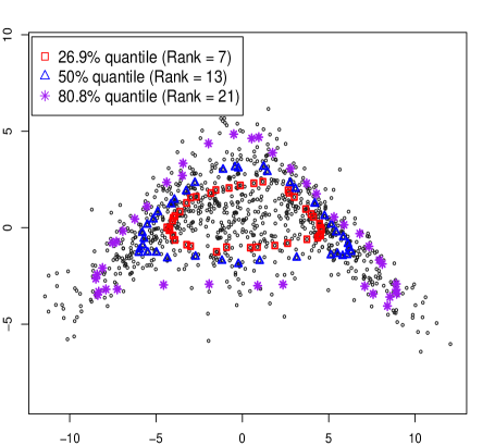
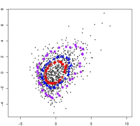
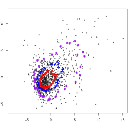
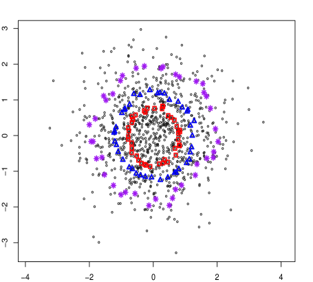
Figure 5: Empirical center-outward quantile contours (probability contents 26.9%, 50 %, and 80%, respectively) computed from $n=1000$ points drawn from the Gaussian mixture (5.2) (top left), the skew-normal and skew-$t_{3}$ described in Section D.2 (top right and bottom left) and, for a comparison, from a standard multivariate normal (bottom right).

Our samples for skew-normal and skew-$t_{3}$ were simulated from the function rmst in the R Package sn by setting $\mbox{\boldmath$\xi$}={\mbox{\boldmath$0$}},{\mbox{\boldmath$\alpha$}}=(5,2)^{\prime},\mbox{\boldmath$\Sigma$}=\left(\begin{array}[]{cc}7&4\\ 4&5\end{array}\right)$. In order to satisfy the classical conditions for M-estimation, we centered the simulated innovations about their mean, a centering which does not affect our R-estimators.

Figure 5 provides scatterplots of samples of size $n=1000$ from the spherical normal, the skew-normal, the skew-$t_{3}$, and the Gaussian mixture described in Section 5.

D.3 Additional numerical results

D.3.1 Large sample

As a complement to Section 5.1, we provide here, for sample size $n=1000$, boxplots of the QMLE, $t_{5}$-QMLE, RMLTSE, and R-estimators (sign test, Spearman, and van der Waerden scores) under skew-normal, skew-$t_{3}$, $t_{3}$ and non-spherical Gaussian innovations with covariance

$$\mbox{\boldmath$\Sigma$}_{4}=\left(\begin{array}[]{cc}5&4\\ 4&4.5\end{array}\right);$$

See Figure 6, 7, 8 and 9, respectively.

Under skew-normal (Figure 6) and skew-$t_{3}$ (Figure 7) innovations, the vdW and Spearman R-estimators are less dispersed than other M-estimators, showing that they are more resistant to skewness. Under spherical $t_{3}$ innovations (Figure 8), outlying observations are relatively frequent and the QMLE is no longer root-$n$ consistent. The RMLTSE does its job as a robustified estimator and slightly outperforms the R-estimators (the weakest of which is the sign-test score one). The non-spherical Gaussian boxplots (Figure 9) show that the vdW and Spearman R-estimators are quite similar to the QMLE.

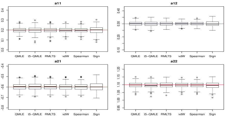
Figure 6: Boxplots of the QMLE, $t_{5}$-QMLE, RMLTSE, and R-estimators (sign test, Spearman, and van der Waerden) under skew-normal innovations (D.2); sample size $n=1000$; $N=300$ replications. The horizontal red line represents the actual parameter value.

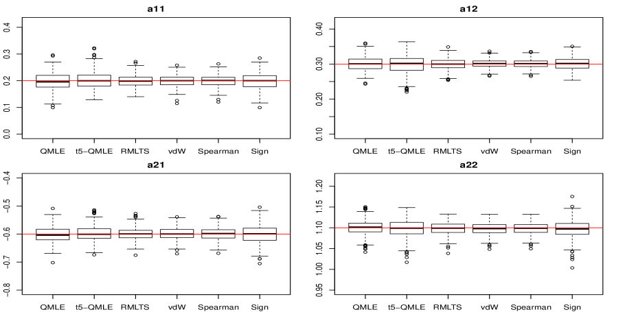
Figure 7: Boxplots of the QMLE, $t_{5}$-QMLE, RMLTSE, and R-estimators (sign test, Spearman, and van der Waerden) under skew-$t_{3}$ innovations (LABEL:St.density); sample size $n=1000$; $N=300$ replications. The horizontal red line represents the actual parameter value.

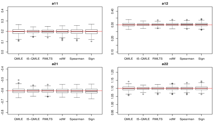
Figure 8: Boxplots of the QMLE, $t_{5}$-QMLE, RMLTSE, and R-estimators (sign test, Spearman, and van der Waerden scores) under $t_{3}$ innovations; sample size $n=1000$; $N=300$ replications. The horizontal red line represents the actual parameter value.

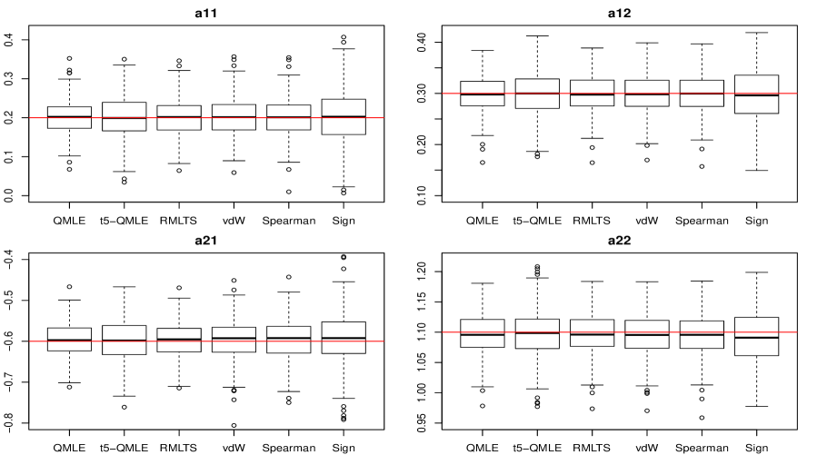
Figure 9: Boxplots of the QMLE, $t_{5}$-QMLE, RMLTSE, and R-estimators (sign test, Spearman, and van der Waerden scores) under non-spherical Gaussian innovations; sample size $n=1000$; $N=300$ replications. The horizontal red line represents the actual parameter value.

D.3.2 Small sample and outliers

For sample size $n=300$, we display here, in Figures 10, 11, 12, 13, and 14, the boxplots of the QMLE, $t_{5}$-QMLE, RMLTSE, and R-estimators (sign test, Spearman, and van der Waerden scores) under the Gaussian mixture (5.2), spherical Gaussian, skew-normal, skew-$t_{3}$, and $t_{3}$, respectively. These pictures complement the boxplots available in Section 5.3, for the additive outlier case.

All boxplots, as well as Table 2 confirm the fact that, while doing equally well under spherical and Gaussian-tailed innovations, as the common practice QMLE, R-estimation is resisting skewness, heavy tails, non-elliptical contours, and the presence of additive outliers, sometimes better even than the robust RMLTSE.

Table 2: The estimated bias ($\times 10^{3}$), MSE ($\times 10^{3}$), and overall MSE ratios of the QMLE, $t_{5}$-QMLE, RMLTSE, and R-estimators under various innovation densities. The sample size is $n=300$; $N=300$ replications.

	Bias ($\times 10^{3}$)				MSE ($\times 10^{3}$)				MSE ratio
	$a_{11}$	$a_{21}$	$a_{12}$	$a_{22}$	$a_{11}$	$a_{21}$	$a_{12}$	$a_{22}$
(Normal)
QMLE	-7.208	-2.006	2.639	-0.870	2.624	2.715	0.543	0.733
$t_{5}$-QMLE	-8.352	-2.065	3.701	-1.071	2.783	2.796	0.580	0.751	0.957
RMLTS	-8.374	-2.423	3.481	-0.706	3.014	2.818	0.607	0.714	0.925
vdW	4.247	-3.994	-2.337	1.076	1.486	1.003	0.985	1.000	1.478
Spearman	5.041	-6.119	-3.395	3.332	1.661	1.204	1.165	1.292	1.243
Sign	6.124	-6.672	-4.254	4.294	2.586	1.839	1.487	0.992	0.958
(Mixture)
QMLE	-3.430	-0.123	4.399	-1.814	2.751	0.550	1.000	0.213
$t_{5}$-MLE	-1.593	0.240	5.467	-1.277	12.295	0.918	4.129	0.461	0.254
RMLTS	-2.459	-0.397	3.997	-1.392	2.707	0.578	1.025	0.220	0.997
vdW	-2.484	-0.007	5.065	1.348	1.427	0.368	0.733	0.379	1.554
Spearman	-2.632	0.742	5.160	1.104	1.329	0.379	0.694	0.332	1.652
Sign	-3.152	-0.066	10.017	1.164	4.313	0.745	2.283	0.566	0.571
(Skew-normal)
QMLE	-9.045	-7.223	5.870	-2.116	3.564	3.308	1.087	1.022
$t_{5}$-QMLE	-7.788	-7.028	6.400	-1.115	4.581	3.992	1.518	1.327	0.787
RMLTS	-9.558	-6.833	5.186	-1.844	3.988	3.574	1.200	1.140	0.907
vdW	-7.086	-1.523	7.358	-5.660	1.879	3.052	0.442	0.706	1.477
Spearman	-6.960	-1.101	7.198	-5.676	1.911	3.109	0.448	0.721	1.451
Sign	-12.525	0.748	10.592	-6.080	3.989	5.962	1.014	1.180	0.740
(Skew-$t_{3}$)
QMLE	-11.108	-4.201	3.932	-1.327	3.148	2.710	1.446	1.209
$t_{5}$-QMLE	1.801	5.000	3.371	-1.652	3.796	2.771	2.269	1.417	0.830
RMLTS	-3.378	0.428	4.358	-1.058	1.918	1.780	1.129	0.833	1.504
vdW	-7.152	0.232	6.544	-3.750	1.718	2.320	0.634	1.240	1.440
Spearman	-5.594	-1.927	6.402	-2.279	1.719	2.388	0.625	1.365	1.396
Sign	-3.380	-1.968	6.469	-0.033	4.816	4.863	1.900	2.054	0.624
($t_{3}$)
QMLE	0.168	-0.844	2.047	-1.063	2.279	2.593	0.647	0.658
$t_{5}$-QMLE	-2.189	0.647	1.176	-1.347	1.160	1.215	0.339	0.343	2.021
RMLTS	-3.538	2.340	0.680	-1.734	1.343	1.377	0.379	0.358	1.787
vdW	-3.426	-0.037	3.681	-6.190	1.435	2.896	0.309	0.816	1.132
Spearman	-2.715	0.208	3.737	-5.768	1.387	2.930	0.306	0.788	1.141
Sign	-2.552	1.297	2.626	-6.454	2.842	5.634	0.564	2.045	0.557
(Additive outliers)
QMLE	-154.990	-149.720	15.327	10.173	27.667	24.982	1.021	1.080
$t_{5}$-QMLE	-110.645	-105.918	12.836	7.714	15.310	13.590	0.859	1.049	1.777
RMLTS	-76.970	-71.918	9.792	4.743	9.931	8.795	0.853	1.042	2.655
vdW	-3.426	-0.037	3.681	-6.190	1.435	2.896	0.309	0.816	10.034
Spearman	-2.715	0.208	3.737	-5.768	1.387	2.930	0.306	0.788	10.118
Sign	-2.552	1.297	2.626	-6.454	2.842	5.634	0.564	2.045	4.939

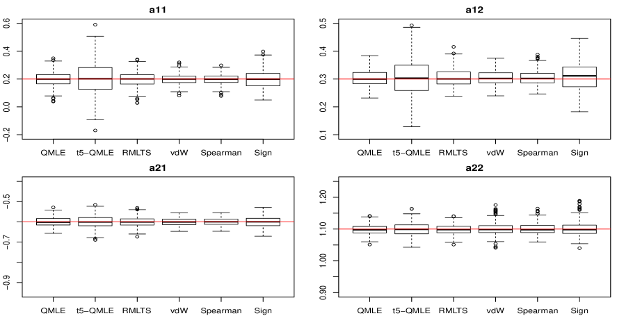
Figure 10: Boxplots of the QMLE, $t_{5}$-QMLE, RMLTSE, and R-estimators (sign test, Spearman, and van der Waerden scores) under Gaussian mixture (sample size $n=300$; $N=300$ replications). The horizontal red line represents the actual parameter value.

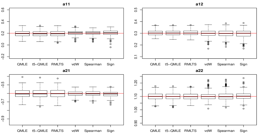
Figure 11: Boxplots of the QMLE, $t_{5}$-QMLE, RMLTSE, and R-estimators (sign test, Spearman, and van der Waerden scores) under spherical Gaussian innovations; sample size $n=300$; $N=300$ replications. The horizontal red line represents the actual parameter value.

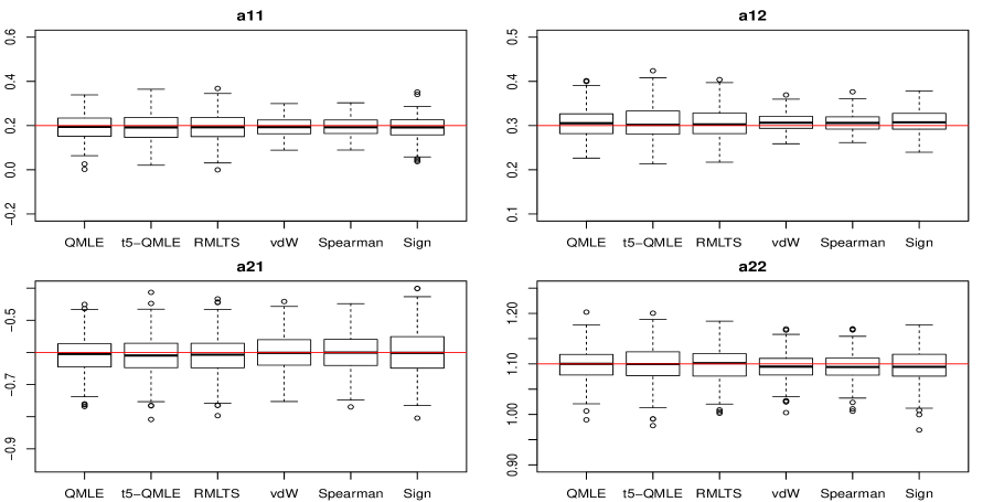
Figure 12: Boxplots of the QMLE, $t_{5}$-QMLE, RMLTSE, and R-estimators (sign test, Spearman, and van der Waerden scores) under skew-normal innovations (D.2); sample size $n=300$; $N=300$ replications. The horizontal red line represents the actual parameter value.

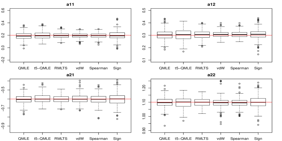
Figure 13: Boxplots of the QMLE, $t_{5}$-QMLE, RMLTSE, and R-estimators (sign test, Spearman, and van der Waerden scores) under skew-$t_{3}$ innovations (LABEL:St.density); sample size $n=300$; $N=300$ replications. The horizontal red line represents the actual parameter value.

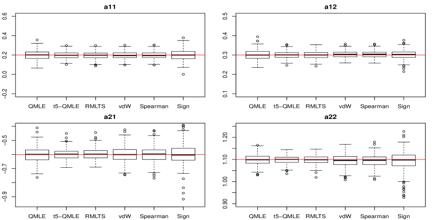
Figure 14: Boxplots of the QMLE, $t_{5}$-QMLE, RMLTSE, and R-estimators (sign test, Spearman, and van der Waerden scores) under spherical $t_{3}$ innovations; sample size $n=300$; $N=300$ replications. The horizontal red line represents the actual parameter value.

D.4 Higher dimension

Due to the rapid growth of their number of parameters, VARMA models are not meant for the analysis of high-dimensional time series (where different approaches are in order—see, e.g., Hallin et al. (2020c)). One may wonder, however, whether the attractive properties of R-estimators extend beyond the bivariate context. We therefore provide here some numerical results in dimension $d=3$.

Consider the three-dimensional VAR($1$) model

$$\left({\mbox{\boldmath$I$}}_{3}-{\mbox{\boldmath$A$}}L\right){\mbox{\boldmath$X$}}_{t}=\mbox{\boldmath$\epsilon$}_{t},\quad t\in{\mathbb{Z}},\vspace{-2mm}$$

with $\mbox{\boldmath$\theta$}^{\prime}:=\text{vec}^{\prime}({\mbox{\boldmath$A$}})=(0.55,0.2,0.13,-0.2,0.5,-0.1,0.1,0.11,0.6)$ satisfying Assumption (A1). We are limiting our investigation to two selected innovation densities: the spherical three-dimensional Gaussian and the Gaussian mixture

$$\frac{3}{8}{\cal N}(\mbox{\boldmath$\mu$}_{1},\mbox{\boldmath$\Sigma$}_{1})+\frac{3}{8}{\cal N}(\mbox{\boldmath$\mu$}_{2},\mbox{\boldmath$\Sigma$}_{2})+\frac{1}{4}{\cal N}(\mbox{\boldmath$\mu$}_{3},\mbox{\boldmath$\Sigma$}_{3}),\vspace{-2mm}$$ (D.4)

with

$$\mbox{\boldmath$\mu$}_{1}=(-5,-5,0)^{\prime},\ \mbox{\boldmath$\mu$}_{2}=(5,5,2)^{\prime},\ \mbox{\boldmath$\mu$}_{3}=(0,0,-3)^{\prime}$$

and

$$\mbox{\boldmath$\Sigma$}_{1}=\begin{bmatrix}7&3&5\\ 3&6&1\\ 5&1&7\end{bmatrix},\ \mbox{\boldmath$\Sigma$}_{2}=\begin{bmatrix}7&-5&-3\\ -5&7&4\\ -3&4&5\end{bmatrix}\text{, and }\mbox{\boldmath$\Sigma$}_{3}=\begin{bmatrix}4&0&0\\ 0&3&0\\ 0&0&1\end{bmatrix}.$$

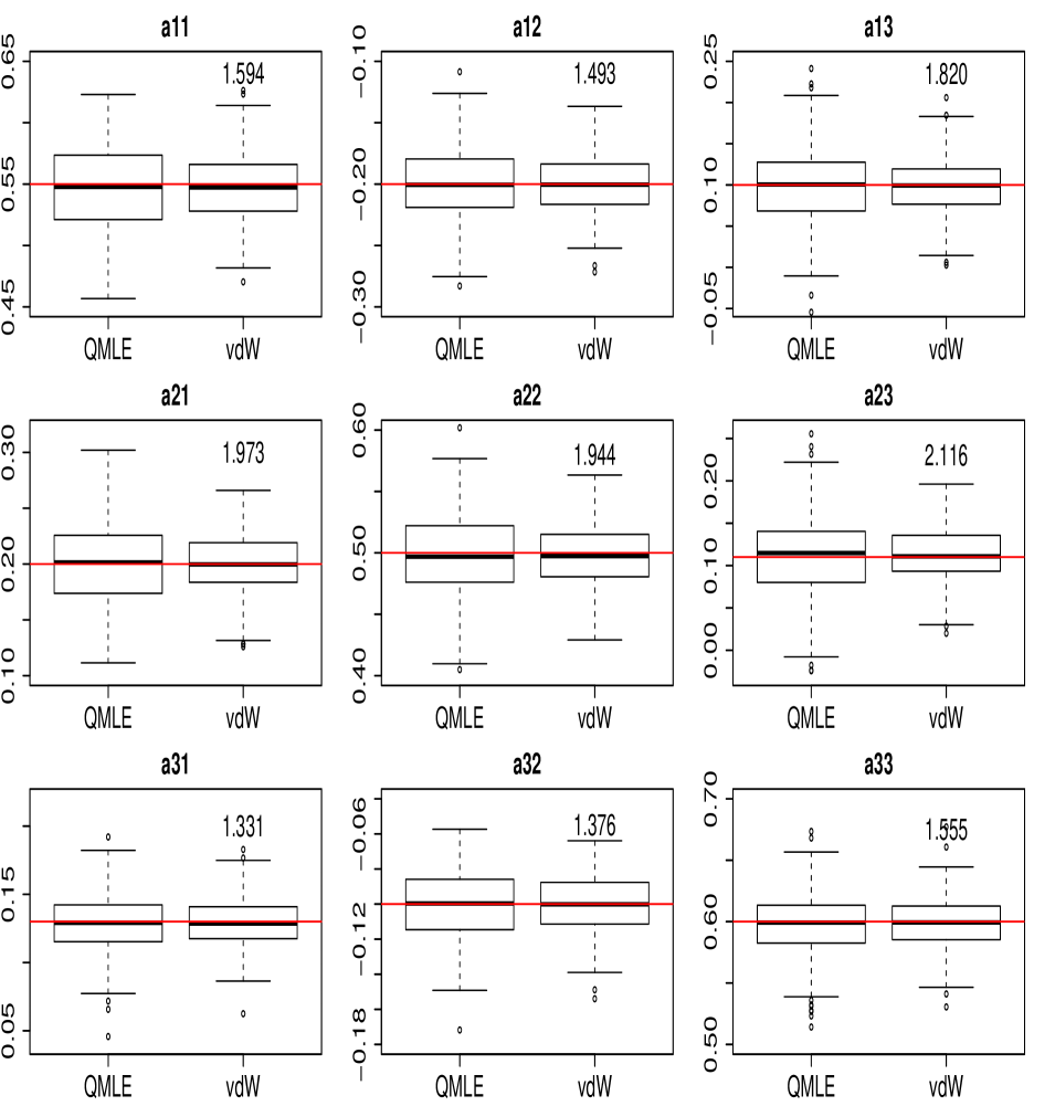
Figure 15: Boxplots of the QMLE and R-estimator (van der Waerden scores) under the Gaussian mixture innovation density (D.4) for $d=3$; sample size $n=1000$; $N=300$ replications. In each panel, the MSE ratio of the QMLE with respect to the R-estimator is reported. The horizontal red line represents the actual parameter value.

For the computation of the center-outward ranks and signs, we used the algorithm described in Appendix C.2 with $n_{R}=15,n_{S}=66,n_{0}=10$. For numerical implementation, we generated regular grids on the sphere via the routine UnitSphere in R package mvmesh, where we refer to for details. The boxplots for the Gaussian mixture and spherical Gaussian innovations are displayed in Figures 15 and 16, respectively. Inspection of Figures 15 and 16 yields the same conclusions as in the bivariate motivating example (Figures 1).

Appendix E Supplementary results for the real-data example

E.1 Estimates for the VARMA(3,1) model

To complement the real data example of Section 6, we provide here the table of estimated coefficients for the macroeconomic time series.

Table 3: The QMLE and R-estimates of $\theta$ in the VARMA($3,1$) fitting of the econometric data (demeaned differenced Hstarts and Mortg series); standard errors are shown in parentheses. The datasets are demeaned differenced Hstarts and Mortg series.

	${\mbox{\boldmath$A$}}_{1}$			${\mbox{\boldmath$A$}}_{2}$			${\mbox{\boldmath$A$}}_{3}$			${\mbox{\boldmath$B$}}_{1}$
QMLE	0.137	0.487		-0.154	-0.199		0.032	0.056		-0.703	-0.490
	(0.265)	(0.353)		(0.284)	(0.130)		(0.171)	(0.072)		(0.258)	(0.350)
	0.596	0.974		0.030	-0.400		0.070	0.110		-0.152	-0.636
	(0.327)	(0.537)		(0.436)	(0.189)		(0.285)	(0.077)		(0.282)	(0.533)
vdW	0.155	0.526		-0.096	-0.181		0.017	0.038		-0.705	-0.527
	(0.141)	(0.088)		(0.122)	(0.079)		(0.133)	(0.062)		(0.088)	(0.071)
	0.561	0.943		0.094	-0.386		0.011	0.128		-0.161	-0.627
	(0.148)	(0.079)		(0.133)	(0.100)		(0.098)	(0.040)		(0.081)	(0.015)
Sign	0.087	0.536		-0.032	-0.198		0.075	-0.044		-0.705	-0.562
	(0.148)	(0.079)		(0.133)	(0.100)		(0.098)	(0.040)		(0.081)	(0.015)
	0.471	1.036		0.107	-0.403		0.035	0.148		-0.161	-0.627
	(0.178)	(0.084)		(0.165)	(0.073)		(0.138)	(0.061)		($<10^{-3}$)	($<10^{-3}$)
Spearman	0.180	0.511		-0.090	-0.180		0.030	0.049		-0.705	-0.537
	(0.066)	(0.033)		(0.092)	(0.046)		(0.113)	(0.049)		($<10^{-3}$)	(0.014)
	0.531	0.946		0.072	-0.374		0.011	0.121		-0.161	-0.627
	(0.124)	(0.054)		(0.115)	(0.075)		(0.112)	(0.042)		($<10^{-3}$)	($<10^{-3}$)

E.2 Impulse response function: a compendium

As explained in Section 6, impulse response functions provide a convenient way of exploring the relation between the components of multiple time series. In particular, it is used to study the impact of changes in one variable on its own future values and those of other time series. For the $d$-dimensional VARMA($p,q$) model in (2.1), the impulse response function can be obtained as follows.

Write (2.1) under the corresponding VMA($\infty$) form

$${\mbox{\boldmath$X$}}_{t}={\mbox{\boldmath$W$}}(L)\mbox{\boldmath$\epsilon$}_{t},\quad t\in\mathbb{Z},$$

where

$${\mbox{\boldmath$W$}}(L):=\sum_{l=0}^{\infty}{\mbox{\boldmath$W$}}_{l}L^{l}=\left({\mbox{\boldmath$I$}}_{d}-\sum_{i=1}^{p}{\mbox{\boldmath$A$}}_{i}L^{i}\right)^{-1}\left({\mbox{\boldmath$I$}}_{d}+\sum_{j=1}^{q}{\mbox{\boldmath$B$}}_{j}L^{j}\right)\mbox{\boldmath$\epsilon$}_{t}$$

with ${\mbox{\boldmath$W$}}_{l}$ being the coefficient at lag $l$.

Now, suppose that we are interested in studying the impact on ${\mbox{\boldmath$X$}}_{t+h}$, $h\geq 0$ of increasing the value at time $t$ of the $k$th series $X_{kt}$, $1\leq k\leq d$ by one unit. Without loss of generality, we can assume $t=0$. Setting ${\mbox{\boldmath$X$}}_{t}={\mbox{\boldmath$0$}}$ for $t\leq 0$, $\mbox{\boldmath$\epsilon$}_{0}={\mbox{\boldmath$e$}}_{k}$ and $\mbox{\boldmath$\epsilon$}_{t}={\mbox{\boldmath$0$}}$ for $t>0$, where ${\mbox{\boldmath$e$}}_{k}$ denotes the $k$th unit vector in the canonical basis of $\mathbb{R}^{d}$, we then have

$${\mbox{\boldmath$X$}}_{0}=\mbox{\boldmath$\epsilon$}_{0}={\mbox{\boldmath$e$}}_{k},\quad{\mbox{\boldmath$X$}}_{1}={\mbox{\boldmath$W$}}_{1}\mbox{\boldmath$\epsilon$}_{0}={\mbox{\boldmath$W$}}_{1,k},\quad{\mbox{\boldmath$X$}}_{2}={\mbox{\boldmath$W$}}_{2}\mbox{\boldmath$\epsilon$}_{0}={\mbox{\boldmath$W$}}_{2,k},\quad...,$$

where ${\mbox{\boldmath$W$}}_{l,k}$ denotes the $k$th column of ${\mbox{\boldmath$W$}}_{l}$. Therefore, the impact under study is reflected in the $k$th column of the coefficient matrix ${\mbox{\boldmath$W$}}_{h}$. For this reason, the coefficient matrices $\{{\mbox{\boldmath$W$}}_{h,k};h\geq 0\}$ are referred to as the coefficients of impulse response functions; see Tsay (2014, Chapter 2 and 3) for further details.

References

- [1] Allal, J., Kaaouachi, A., and Paindaveine, D. (2001) R-estimation for ARMA models. Journal of Nonparametric Statistics, 13:6, 815–831.
- [2] Andreou, E. and Werker, B. (2015). Residual-based rank specification tests for AR-GARCH type models. Journal of Econometrics, 185, 305–331.
- [3] Andrews, B. (2008). Rank-based estimation for autoregressive moving average time series models. Journal of Time Series Analysis, 29, 51–73.
- [4] Andrews, B. (2012). Rank-based estimation for GARCH processes. Econometric Theory, 28, 1037–1064.
- [5] Azzalini, A. and Capitanio, A. (2003). Distributions generated by perturbation of symmetry with emphasis on a multivariate skew t-distribution. Journal of the Royal Statistical Society Series B, 65, 367–389.
- [6] Azzalini, A. and Dalla Valle, A. (1996). The multivariate skew-normal distribution. Biometrika, 83, 715–726.
- [7] Bickel, P.J., Klaassen, C.A.J., Ritov, Y., and Wellner, J.A. (1993). Efficient and Adaptive Estimation for Semiparametric Models. Johns Hopkins University Press, Baltimore, MD.
- [8] Boeckel, M., Spokoiny, V., and Suvorikova, A. (2018). Multivariate Brenier cumulative distribution functions and their application to nonparametric testing, arXiv:1809.04090.
- [9] Brockwell, P. and Davis, R. (2006). Time Series: Theory and Methods (2nd edition). Springer, New York.
- [10] Carlier, G., Chernozhukov, V., and Galichon, A. (2016). Vector quantile regression, Ann. Statist., 44, 1165–1192.
- [11] Cassart, D., Hallin, M., and Paindaveine, D. (2010). On the estimation of cross-information quantities in R-estimation. In J. Antoch, M. Hušková and P.K. Sen, Eds: Nonparametrics and Robustness in Modern Statistical Inference and Time Series Analysis: A Festschrift in Honor of Professor Jana Jurečková, I.M.S., 35–45.
- [12] Chernozhukov, V., Galichon, A., Hallin, M., and Henry, M. (2017). Monge- Kantorovich depth, quantiles, ranks, and signs, Annals of Statistics, 45, 223–256.
- [13] Croux, C. and Joossens, K. (2008). Robust estimation of the vector autoregressive model by a least trimmed squares procedure. COMPSTAT 2008, 489-501.
- [14] Cuesta-Albertos, J.A. and Matrán, C. (1989). Notes on the Wasserstein metric in Hilbert spaces. Ann. Probab., 17, 1264–1276.
- [15] Dick, J. and Pillichshammer, F. (2014). Discrepancy theory and quasi-Monte Carlo integration, in W. Chen, A. Sirvastava and G. Travaglini, Eds, A Panorama of Discrepancy Theory, 539-620, Springer, New York.
- [16] Engle, R. W. (2002). Dynamic conditional correlation, Journal of Business & Economic Statistics, 20:3, 339-350.
- [17] Figalli, A. (2018). On the continuity of center-outward distribution and quantile functions, Nonlinear Analysis, 177, part B, 413-421.
- [18] Galichon, A. (2016). Optimal Transport Methods in Economics. Princeton University Press.
- [19] Galichon, A. (2017). A survey of some recent applications of optimal transport methods to econometrics, Econometrics Journal, 20:C1–C11.
- [20] Garel, B. and Hallin, M. (1995). Local asymptotic normality of multivariate ARMA processes with a linear trend, Annals of the Institute of Statistical Mathematics, 3, 551-579.
- [21] Hájek, J. and Šidák, (1967). Theory of Rank Tests. New York: Academic Press.
- [22] Hájek, J., Šidák, Z., and Sen, P.K. (1999). Theory of Rank Tests, 2nd edition. San Diego: Academic Press.
- [23] Hallin, M. (1986). Non-stationary -dependent processes and time-varying moving-average models: invertibility properties and the forecasting problem. Advances in Applied Probability, 18, 170-210.
- [24] Hallin, M. (2017). On distribution and quantile functions, ranks and signs in . ECARES WP. Available at https://ideas.repec.org/p/eca/wpaper/2013-258262.html.
- [25] Hallin, M., del Barrio, E., Cuesta-Albertos, J., and Matrán, C. (2020a). Center-outward distribution and quantile functions, ranks, and signs in dimension : a measure transportation approach, Annals of Statistics, in press.
- [26] Hallin, M., Hlubinka, D., and Hudecová, S. (2020b). Efficient center-outward rank tests for multiple-output regression and MANOVA. Manuscript in progress.
- [27] Hallin, M., Ingenbleek, J-Fr., and Puri, M.L. (1985). Linear serial rank tests for randomness against ARMA alternatives. Annals of Statistics, 13, 1156–1181.
- [28] Hallin, M. and La Vecchia, D. (2017). R-estimation in semiparametric dynamic location-scale models. Journal of Econometrics, 2, 233–247.
- [29] Hallin, M. and La Vecchia, D. (2019). A simple R-estimation method for semiparametric duration models. Journal of Econometrics. Forthcoming.
- [30] Hallin, M., Oja, H., and Paindaveine, D. (2006). Semiparametrically efficient rank-based inference for shape: II Optimal R-estimation of shape. Annals of Statistics, 34, 2757–2789.
- [31] Hallin, M. and Paindaveine, D. (2002a). Optimal tests for multivariate location based on interdirections and pseudo-Mahalanobis ranks. Annals of Statistics, 30, 1103–1133.
- [32] Hallin, M. and Paindaveine, D. (2002b). Optimal procedures based on interdirections and pseudo-Mahalanobis ranks for testing multivariate elliptic white noise against ARMA dependence. Bernoulli, 8, 787–815.
- [33] Hallin, M. and Paindaveine, D. (2004). Rank-based optimal tests of the adequacy of an elliptic VARMA model. Annals of Statistics, 32, 2642–2678.
- [34] Hallin, M. and Paindaveine, D. (2005). Asymptotic linearity of serial and nonserial multivariate signed rank statistics. Journal of Statistical Planning and Inference, 136, 1–32.
- [35] Hallin, M. and Puri, M.L. (1994). Aligned rank tests for linear models with autocorrelated errors. Journal of Multivariate Analysis, 50, 175–237.
- [36] Hallin, M., van den Akker, R., and Werker, B. (2015). On quadratic expansions of log-likelihoods and a general asymptotic linearity result. In M. Hallin, D. Mason, D. Pfeifer, and J. Steinebach Eds, Mathematical Statistics and Limit Theorems, Festschrift in Honor of Paul Deheuvels, Springer, 147–166.
- [37] Hallin, M. and Werker, B. (2003). Semiparametric efficiency, distribution-freeness, and invariance. Bernoulli, 9, 137–165.
- [38] Hodges, J. and Lehmann, E. L. (1956). The efficiency of some nonparametric competitors of the t-test. Annals of Mathematical Statistics, 34, 324–335.
- [39] Jaeckel, L. A. (1972). Estimating regression coefficients by minimizing the dispersion of the residuals. Annals of Mathematical Statistics, 43, 1449–1458.
- [40] Judd, K.L. (1998). Numerical Methods in Economics, MIT Press, Cambridge, MA.
- [41] Jurečková, J. (1969). Asymptotic linearity of a rank statistic in regression parameter. Annals of Mathematical Statistics, 40, 1889–1900.
- [42] Jurečková, J. (1971). Nonparametric estimate of regression coefficients. Annals of Mathematical Statistics, 42, 1328–1338.
- [43] Koul, H. (1971). Asymptotic behavior of a class of confidence regions based on ranks in regression. Annals of Mathematical Statistics, 42, 466–476.
- [44] Koul, H. and Ossiander, M. (1994). Weak convergence of randomly weighted dependent residual empiricals with applications to autoregression. Annals of Statistics, 22, 540–562.
- [45] Koul, H. L. and Saleh, A. M. E. (1993). R-estimation of the parameters of autoregressive AR() models. Annals of Statistics, 21, 534–551.
- [46] Kolouri, S., Park, S. R., Thorpe, M., Slepcev, D., and Rohde, G. K. (2017). Optimal mass transport: Signal processing and machine-learning applications, IEEE Signal Processing Magazine, 34:43–59.
- [47] Kreiss, J.-P. (1987). On adaptative estimation in stationary ARMA processes, Annals of Statistics, 15, 112–133.
- [48] Liu, R. Y. (1992). Data depth and multivariate rank tests, in Y. Dodge, Ed., Statistics and Related Methods. North-Holland, Amsterdam, 279–294.
- [49] Le Cam, L. and Yang, G. L. (2000). Asymptotics in Statistics : some basic concepts (2nd ed.). New York: Springer.
- [50] Liu, R.Y. and Singh, K. (1993). A quality index based on data depth and multivariate rank tests, J. Amer. Statist. Assoc. 88, 257–260.
- [51] Mukherjee, K. (2007). Generalized R-estimators under conditional heteroscedasticity. Journal of Econometrics, 141, 383–415.
- [52] Maronna, R., Martin D., Yohai V., and Salibian-Barrera M. (2019), Robust Statistics: Theory and Methods (with R), Wiley.
- [53] Mukherjee, K. and Bai, Z. (2002). R-estimation in autoregression with square-integrable score function. Journal of Multivariate Analysis, 81, 167–186.
- [54] Niederreiter, H. (1992). Random Number Generation and Quasi-Monte Carlo Methods. CBMS-NSF Regional Conference Series in Applied Mathematics, vol. 63, SIAM, Philadelphia, PA.
- [55] Oja, H. (2010). Multivariate Nonparametric Methods with R: an approach based on spatial signs and ranks. Springer, New York.
- [56] Panaretos, V. M. and Zemel, Y. (2019). Statistical aspects of Wasserstein distances. Annual Review of Statistics and its Application, 6:405–431.
- [57] Peyré, G. and Cuturi, M. (2019). Computational optimal transport with applications to Data Science. Foundations and Trends® in Machine Learning, 11(5-6):355–607.
- [58] Puri, M.L. and Sen, P.K. (1971). Nonparametric Methods in Multivariate Analysis. John Wiley & Sons, New York.
- [59] Rachev, S.T. and Rüschendorf, L. (1998). Mass Transportation Problems I and II, Springer, New York.
- [60] R Core Team (2019). R: A language and environment for statistical computing. R Foundation for Statistical Computing, Vienna, Austria. URLhttp://www.R-project.org/.
- [61] Santner, T.J., Williams, B.J. and Notz, W.I. (2003). The Design and Analysis of Computer Experiments, Springer-Verlag, New York.
- [62] Terpstra, J.T., McKean, J. W., and Naranjo, J. D. (2001). GR-estimates for an autoregressive time series. Statistics & Probability Letters, 51, 165–172.
- [63] Tsay, R.S. (2014). Multivariate Time Series Analysis with R and Financial Applications. Hoboken, New Jersey: Wiley.
- [64] van der Vaart, A. (1998). Asymptotic Statistics. Cambridge University Press.
- [65] van Eeden, C. (1972). An analogue, for signed rank statistics, of Jurečková’s asymptotic linearity theorem for rank statistics. Annals of Mathematical Statistics, 43, 791–802.
- [66] Villani, C. (2009). Optimal Transport: Old and New, Springer-Verlag, Berlin.