Toward 3D Object Reconstruction from Stereo Images

Abstract

Inferring the 3D shape of an object from an RGB image has shown impressive results, however, existing methods rely primarily on recognizing the most similar 3D model from the training set to solve the problem. These methods suffer from poor generalization and may lead to low-quality reconstructions for unseen objects. Nowadays, stereo cameras are pervasive in emerging devices such as dual-lens smartphones and robots, which enables the use of the two-view nature of stereo images to explore the 3D structure and thus improve the reconstruction performance. In this paper, we propose a new deep learning framework for reconstructing the 3D shape of an object from a pair of stereo images, which reasons about the 3D structure of the object by taking bidirectional disparities and feature correspondences between the two views into account. Besides, we present a large-scale synthetic benchmarking dataset, namely StereoShapeNet, containing 1,052,976 pairs of stereo images rendered from ShapeNet along with the corresponding bidirectional depth and disparity maps. Experimental results on the StereoShapeNet benchmark demonstrate that the proposed framework outperforms the state-of-the-art methods.

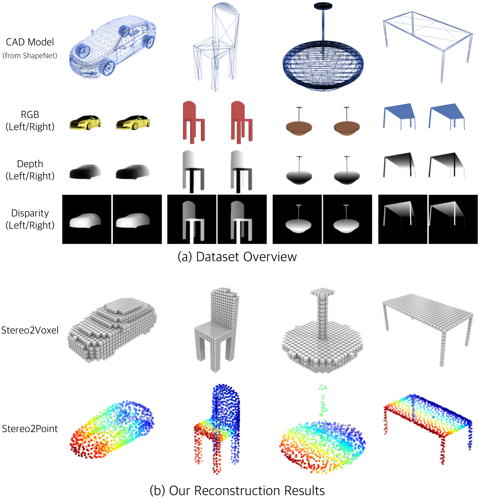
Figure 1: (a) Our dataset provides over 1 million pairs of stereo images along with the corresponding 3D volumes and point clouds, bidirectional depth and disparity maps. (b) We propose two networks to generate a 3D volumes or a point clouds from stereo images, respectively.

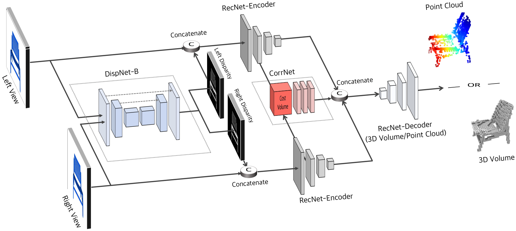
Figure 2: An overview of the proposed methods that recover the 3D volume or point cloud of an object from a pair of stereo images. Note that the weights of the encoders in RecNet are shared between the two views.

Introduction

Recovering the complete 3D shape of an object from a single image is often described as an ill-posed and inherently ambiguous problem because the partial observation of the object can be theoretically associated with an infinite number of possible 3D models. Data-driven methods (?; ?) can recover the 3D shape of an object from a single image and have shown impressive results. However, as demonstrated by (?), these methods do not reason about the 3D structure from a single image and rely primarily on recognizing the most similar 3D model from the training set to solve the problem, which may lead to low-quality reconstructions for unseen objects.

It has been proved that depth information benefits object reconstruction (?; ?). RGB-D cameras have brought about a profound advancement of object reconstruction because of the use of depth recorded by the depth camera. However, depth cameras are sensitive to illumination and the depth accuracy degenerates rapidly with the decreasing illumination power (?). Another way to obtain depth is to estimate depth from an RGB image. However, monocular depth estimation itself is challenging because of structural variations and object occlusions in most scenes (?). In contrast, it is more reliable to estimate depth or disparity from stereo images. In addition, introducing stereo images also enables the networks to explore the dense feature correspondences between two correlated views, which are beneficial to infer the 3D structure of the object. Despite the above congenital advantages, the surge in dual-lens smartphones and robots also sheds light on 3D object reconstruction from stereo images.

In this paper, we propose a new framework for reconstructing the complete 3D shape of an object from a pair of stereo images. To explicitly infer the 3D structure of the object, the proposed framework explores the bidirectional disparities and feature correspondences between two views of stereo images. As illustrated in Figure 2, it consists of three sub-networks: DispNet-B, CorrNet, and RecNet. DispNet-B estimates the bidirectional disparities from a pair of stereo images, which are fed, along with the stereo RGB images, into the encoder of RecNet. CorrNet finds dense feature correspondences between the stereo image pairs. The decoder of RecNet generates the 3D volume or point cloud of an object from concatenated feature maps.

Currently, there is no particular dataset for training and benchmarking stereo 3D object reconstruction in the deep learning community. Therefore, we construct a large-scale synthetic dataset rendered from ShapeNet, named StereoShapeNet, using the open-source 3D creation suite Blender. In particular, it includes 1,052,976 pairs of stereo RGB images and the corresponding ground truth for the 3D model, bidirectional depth as well as disparity maps.

The contributions can be summarized as follows:

• We study the stereo 3D object reconstruction problem with deep learning. We propose a framework that exploits the disparities and feature correspondences of a pair of stereo images to reconstruct the 3D shape of an object in forms of a 3D volume and point clouds.

• We release a large-scale benchmarking dataset, namely StereoShapeNet, containing over 1M pairs of stereo images rendered from ShapeNet along with the corresponding bidirectional depth and disparity maps, which is the first benchmark for stereo 3D object reconstruction.

• Experimental results on the StereoShapeNet dataset demonstrate that the proposed method outperforms state-of-the-art methods in both point cloud and 3D volume reconstruction.

Related Work

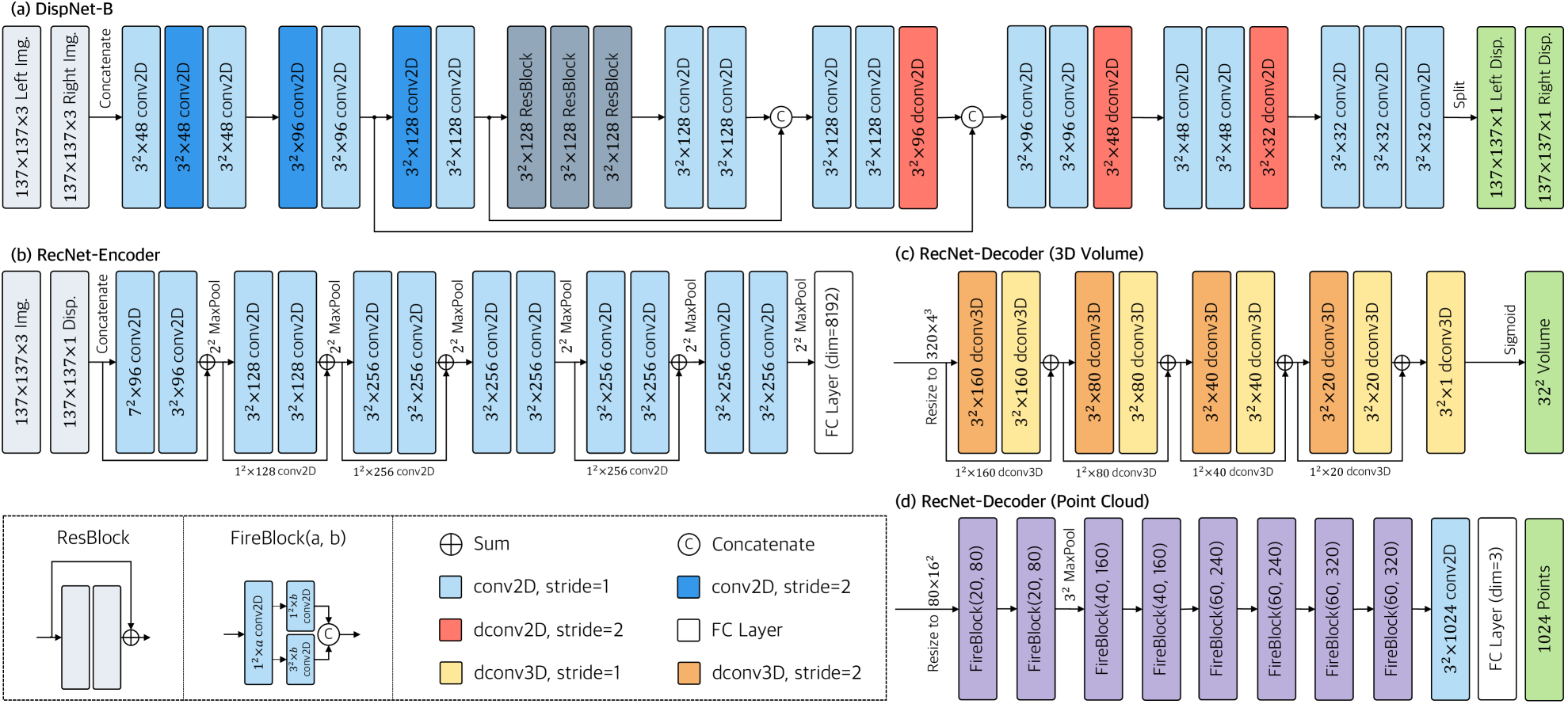
Figure 3: The network architecture of Stereo2Voxel and Stereo2Point. The difference between Stereo2Voxel and Stereo2Point is that Stereo2Voxel uses a RecNet-Decoder (3D Volume) while Stereo2Point adopts a RecNet-Decoder (Point Cloud). The rest of the components are the same in both networks.

Single-view 3D Reconstruction. Early works such as ShapeFromX (?; ?) make strong assumptions about the shape or the environment lighting conditions. Boosted by large-scale datasets of 3D CAD models such as ShapeNet (?), data-driven single-view 3D reconstruction methods (?; ?) are able to reconstruct the 3D shape of an object based on only one image without assumptions about the environment. Tatarchenko et al. (?) propose an octree-based voxel representation and generate a 3D shape from a single image. PSGN (?) recovers the point cloud of an object from a single image.

Multi-view 3D Reconstruction. Classical 3D reconstruction methods, such as SfM and vSLAM, require a collection of RGB images to reconstruct the 3D shape of an object. The geometric shape is recovered by dense feature extraction and matching (?), or by directly minimizing reprojection errors (?) from color images. Recently, deep neural networks are designed to recover the 3D shape of an object from multiple images (?; ?). 3D-R2N2 (?) uses a gated recurrent unit (GRU) (?) to infer 3D shape from single or multiple images and achieve impressive results. In Pix2Vox (?), the context-aware fusion is incorporated to select high-quality reconstructions for each part from different coarse 3D volumes.

RGB-D 3D Reconstruction. Several representative works (?; ?) reconstruct the 3D shape of an object from RGB-D images by shape completion. Traditional reconstruction approaches use interpolation techniques (e.g., plane fitting, Laplacian hole filling) to infer the underlying 3D structure (?; ?). 3D-RecNet++ (?) generates a complete and fine-grained 3D structure from a single depth view with deep neural networks.

The Method

Problem and Notations

Our goal is to reconstruct the 3D shape of an object from a pair of stereo RGB images. The reconstructed 3D shape is represented in two forms: a 3D volume and a point cloud, as shown in Figure 1. Assume $I^{L}$ and $I^{R}$ indicate the left and right view of an object. The ground truth disparity maps for the left and right views are denoted as $D^{L}$ and $D^{R}$. The estimated disparity maps are represented by $\hat{D}^{L}$ and $\hat{D}^{R}$, respectively. Let $V$ and $\hat{V}$ be the ground truth and predicted 3D volumes, respectively. The ground truth and predicted point cloud are denoted by $P=\{(x_{i},y_{i},z_{i})\}_{i=1}^{n_{gt}}$ and $\hat{P}=\{(x_{i},y_{i},z_{i})\}_{i=1}^{n_{p}}$, respectively.

Network Architectures

There are two alternative implementations for generating 3D volumes and point clouds, named Stereo2Voxel and Stereo2Point, respectively. The detailed network architectures are shown in Figure 3. Both of them consist of three sub-networks: DispNet-B, RecNet, and CorrNet. First, DispNet-B predicts bidirectional disparities from a pair of stereo images. Second, the encoder of RecNet generates two feature vectors of size $8192$ from stereo images and their disparities. Third, the feature maps from the 3rd convolutional layer of the encoder in RecNet are forwarded to CorrNet, which finds the feature correspondences between the two images and produces a feature vector of size $4096$. Finally, the decoder of RecNet reconstructs a 3D volume or a point cloud from the concatenated feature vectors generated from the encoder of RecNet and CorrNet. In RecNet, the decoders for Stereo2Voxel and Stereo2Point are different. Stereo2Voxel outputs a 3D volume with a resolution of $32^{3}$ while Stereo2Point outputs an unordered point set containing 1024 points in the object’s canonical view.

DispNet-B. DispNet-B is to compute the bidirectional disparities. The U-Net based structure of DispNet-B is shown in Figure 3 (a). The encoder outputs feature maps with $\frac{1}{8}\times\frac{1}{8}$ of the input size. Afterward, the following decoder produces the full resolution disparities by three transposed convolutional layers. Different from DispNet (?), the proposed DispNet-B predicts bidirectional disparities in only one forward computation. It has been proved that bidirectional prediction is better than unidirectional prediction in optical flow estimation (?). DispNet-B is 6% size of DispNet because it takes a small number of channels for each layer. Therefore, DispNet-B is computationally efficient and 4 times faster than DispNet. The output of DispNet-B is bidirectional disparities with the same size as the inputs.

RecNet. RecNet produces 3D volumes and point clouds by taking stereo RGB images and the corresponding disparities as input. Inspired by the fact that residual connections between convolutional layers accelerate the optimization process (?), the encoder of RecNet uses the residual block as the building block. To match the number of channels after convolutions, we add a $1\times 1$ convolutional layer for residual connections. There are two versions of decoders to transform feature vectors into 3D volumes (Stereo2Voxel) and point clouds (Stereo2Point), respectively, as shown in Figure 3 (c) and (d). The input feature vectors of the decoders are concatenated of the feature vectors from the encoder of RecNet and CorrNet.

To generate 3D volumes, the decoder of RecNet contains nine transposed 3D convolutional layers that upsample the feature maps to the size of $32^{3}$. The final feature map is passed to a sigmoid layer and produces the probabilities of each 3D occupancy grid. Similar to the encoder of RecNet, there are residual connections between the transposed 3D convolutional layers for improving efficiency.

To produce point clouds, the decoder consists of eight Fire modules (?) and a fully connected layer. Following PSGN (?), we produce a matrix of size $1024\times 3$, which corresponds to the coordinates of $1024$ points. To reduce the size of the decoder, we adopt several Fire modules to replace the massive transposed convolutional layers and fully connected layers. Each Fire block contains a squeeze convolutional layer (which has only $1\times 1$ filters), fed into an expand layer that has a mix of $1\times 1$ and $3\times 3$ convolution filters. Fire blocks replace several $3\times 3$ filters with $1\times 1$ filters and decrease the number of input channels to $3\times 3$ filters. Consequently, the RecNet is 28% size of PSGN.

CorrNet. As stated above, CorrNet is introduced to find the feature correspondences between the two views. The feature correspondences are computed by forming a cost volume that preserves the knowledge of geometry of stereo vision. Following GC-Net (?), the cost volume is of dimensionality height$\times$width$\times$(max disparity / shift intervals)$\times$channels and formed by stacking left and right feature maps with shift intervals. The cost volume allows the network to perform multiplicative patch comparisons between two feature maps by aggregating feature information along the disparity dimension as well as spatial dimensions.

We propose to use a 3D-CNN for further feature matching. In 3D-CNN, there are nine sets of 3D convolutional layers with output channels of $128$, along with the corresponding batch normalization layers and ReLU layers. The convolutional layers are with kernel sizes of $3\times 3\times 3$ except for the first layer with a kernel size of $1\times 1\times 1$. 3D-CNN is lastly followed by a $1\times 1\times 1$ convolutional layer with an output channel of $1$ and a $1\times 1$ convolutional layer whose output channel is $1$. Both of them are followed by a batch normalization layer and a ReLU activation. The output of 3D-CNN is then flattened and passed to a fully connected layer with a dimension of $4096$.

Loss Functions

There are three loss functions for predicting disparity maps, 3D volumes, and point clouds, respectively.

Disparity Loss. We adopt Mean Square Error (MSE) loss to measure the difference between the estimated disparities and the corresponding ground truth. More specifically, the disparity loss is defined as

$$\mathcal{L}_{disp}=\frac{1}{HW}\sum\left[||\hat{D}^{L}-D^{L}||^{2}+||\hat{D}^{R}-D^{R}||^{2}\right]$$ (1)

where $H$ and $W$ represent the height and width of disparity, respectively.

3D Volume Loss. The loss function for predicting 3D volume is defined as the sum value of the voxel-wise binary cross entropies between the reconstructed object and the ground truth. More formally, it can be defined as

$$\mathcal{L}_{vol}=\frac{1}{n_{vox}}\sum\left[V\log(\hat{V})+(1-V)\log(1-\hat{V})\right]$$ (2)

where $n_{vox}$ denotes the number of voxels in the 3D volume.

Point Cloud Loss. We use the Chamfer Distance to measure the point-to-point similarity between two point clouds following (?). The Chamfer Distance (CD) is defined as

$$\mathcal{L}_{cd}=\frac{1}{n_{gt}}\sum_{p\in P}\min_{q\in\hat{P}}||p-q||^{2}_{2}+\frac{1}{n_{p}}\sum_{p\in\hat{P}}\min_{q\in P}||p-q||^{2}_{2}$$ (3)

Experiments

Table 1: Reconstruction results from stereo RGB images on StereoShapeNet. Intersection over union (IoU) and Chamfer distance (CD) are adopted to evaluate the performance for voxel reconstruction and point cloud reconstruction, respectively. The best number for each category is highlighted in bold. Note that PSGN and PSGN^∗ take object masks as an additional input. LSM takes extrinsic camera parameters as an additional input.

Category	Voxel Reconstruction (IoU, Resolutions of $32^{3}$)					Point Cloud Reconstruction (CD $\times 10^{-3}$, 1024 Points)
	Matryoshka	Matryoshka∗	Pix2Vox	LSM	Stereo2Voxel	PSGN	PSGN∗	AtlasNet	AtlasNet∗	Stereo2Point
airplane	0.557	0.535	0.686	0.621	0.709	0.826	0.699	0.807	0.796	0.534
bench	0.524	0.473	0.566	0.517	0.622	1.789	1.695	1.996	1.796	1.182
cabinet	0.766	0.763	0.754	0.691	0.784	2.360	1.853	1.756	1.692	1.229
car	0.827	0.810	0.811	0.796	0.830	1.295	0.882	1.045	1.036	0.779
chair	0.559	0.514	0.604	0.595	0.669	2.004	1.594	1.837	1.858	1.267
display	0.635	0.614	0.586	0.547	0.692	2.815	2.238	2.386	2.146	1.356
lamp	0.424	0.411	0.449	0.469	0.521	3.973	3.038	4.142	4.118	3.001
speaker	0.697	0.727	0.658	0.670	0.701	3.868	2.691	2.839	2.869	2.124
rifle	0.540	0.557	0.652	0.682	0.690	0.790	0.763	0.818	0.874	0.524
sofa	0.702	0.679	0.714	0.651	0.770	2.625	2.086	1.664	1.656	1.199
table	0.559	0.503	0.570	0.566	0.635	1.889	1.500	1.892	1.916	1.337
telephone	0.759	0.847	0.831	0.694	0.866	1.445	1.158	1.156	1.250	0.896
watercraft	0.587	0.595	0.558	0.592	0.645	2.029	1.495	1.712	1.524	1.027
Overall	0.626	0.603	0.652	0.632	0.702	1.916	1.493	1.704	1.689	1.185

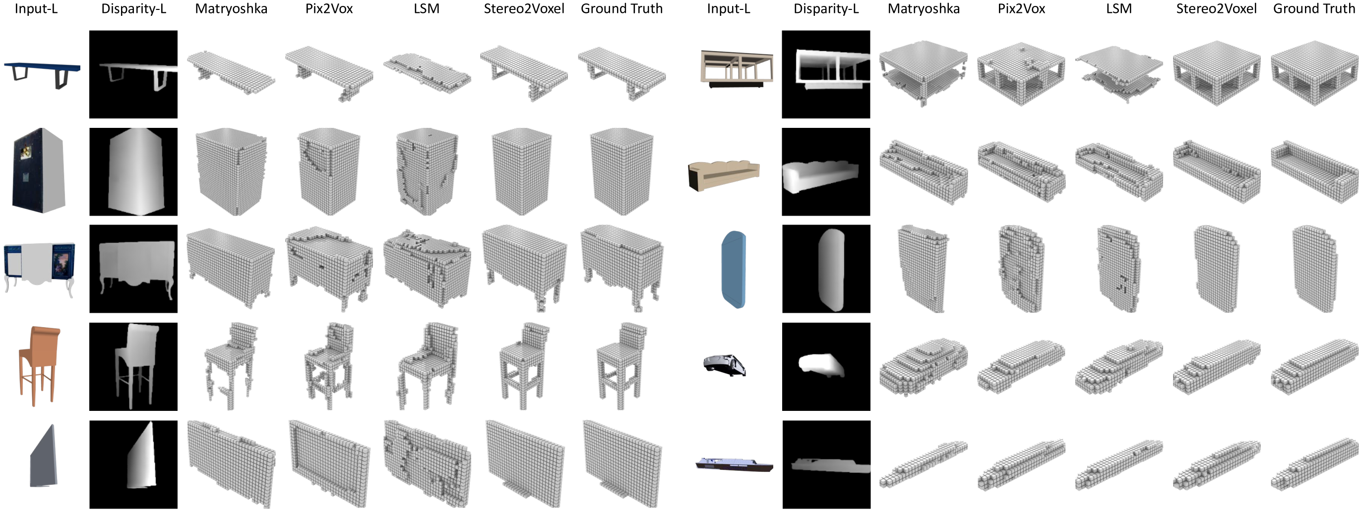
Figure 4: The 3D volumes reconstructed from stereo images on the StereoShapeNet dataset. Input-L represents the left-view of the input images. Disparity-L denotes the left-view of the estimated disparity by DispNet-B.

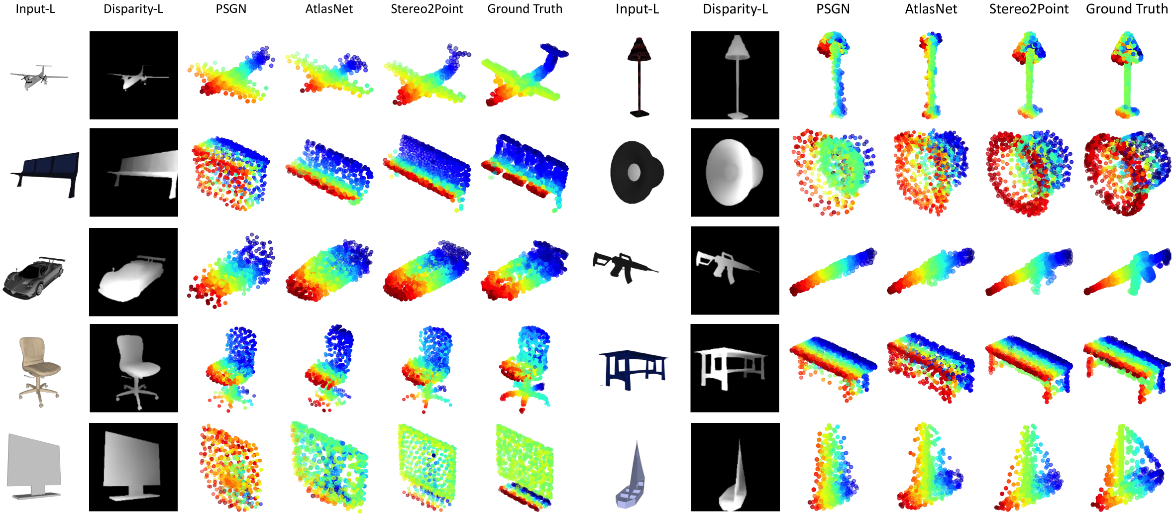
Figure 5: The point cloud reconstructed from stereo images on the StereoShapeNet dataset. Input-L represents the left-view of the input imag‘33es. Disparity-L denotes the left-view of the estimated disparity by DispNet-B. Note that PSGN takes object masks as an additional input.

Dataset and Metrics

Dataset. We present a large-scale synthetic dataset, named StereoShapeNet. We use the 3D models in the ShapeNet dataset (?) to generate stereo images, depth maps, and disparity maps for all our experiments. Specifically, we use a subset of ShapeNet consisting of 44k 3D models from 13 major categories following the settings of 3D-R2N2 (?). We generate a large set of stereo renderings for the models sampled from a viewing sphere $\theta_{az}\in[0,360)$ and $\theta_{el}\in[-20,30]$ degrees with the open-source 3D computer graphics toolset Blender. We also render the depth images as well as disparities corresponding to each rendered image. The images are with resolutions of $224\times 224$. In the Blender, the stereo camera is of a virtual focal length of 35mm and a simulated sensor of size 32mm wide. The baseline of the stereo camera is 130mm. In total, the StereoShapeNet contains 1,052,976 pairs of stereo images with the corresponding bidirectional depth and disparity maps. For volumetric ground truth, we voxelize each 3D CAD model at a resolution of $32^{3}$. For the ground truth of point clouds, we uniformly densify 3D points on the surfaces to generate 16,384 points for each 3D model.

Evaluation Metrics. To evaluate the quality of the output from Stereo2Voxel, we binarize the probabilities at a fixed threshold of $0.4$ and use intersection over union (IoU) as the similarity measure. More specifically,

$${\rm IoU}=\frac{\sum_{i,j,k}{\rm I}(\hat{V}^{(i,j,k)}>t){\rm I}(V^{(i,j,k)})}{\sum_{i,j,k}{\rm I}\left[{\rm I}(\hat{V}^{(i,j,k)}>t)+{\rm I}(V^{(i,j,k)})\right]}$$ (4)

where $\hat{V}^{(i,j,k)}$ and $V^{(i,j,k)}$ represent the predicted occupancy probability and the ground truth at $(i,j,k)$, respectively. ${\rm I}(\cdot)$ is an indicator function and $t$ denotes a voxelization threshold. Higher IoU values indicate better reconstruction results.

To evaluate the similarity between the ground truth and the generated point clouds from Stereo2Point, we introduce Chamfer Distance (CD) following (?) (Equation 3). The lower the CD value is, the closer the prediction is to the ground truth.

Implementation Details

We use $137\times 137$ RGB images as input to train the proposed methods with a batch of $20$. The 3D volume generated by Stereo2Voxel is $32^{3}$ in size. Following (?), $n_{p}$ and $n_{gt}$ are pre-assigned to $1024$ and $16384$, respectively. The shift interval in CorrNet is set to $1$. We implement our network in PyTorch using an Adam (?) optimizer with $\beta_{1}=0.9$ and $\beta_{2}=0.999$. The initial learning rate is set to $10^{-4}$ and decayed by 2 after 300 epochs. The optimization is set to stop after 500 epochs.

Reconstruction results from Synthetic Images

To evaluate the performance of the proposed methods in handling synthetic images, we compare our methods against several state-of-the-art methods on the StereoShapeNet testing set. We fine-tune all competitive methods on the StereoShapeNet dataset and test them with the same pair of stereo images for each object. For voxel reconstruction methods, we compare Stereo2Voxel with Matryoshka Network (?) and Pix2Vox (?) that are used for single-view and multi-view 3D object reconstruction, respectively. To further demonstrate the superior reconstruction ability of the proposed methods, we compare Stereo2Voxel with a MVS method LSM (?). For point cloud reconstruction, we compare Stereo2Point with PSGN (?) and AtlasNet (?). For single-view reconstruction methods, the left view of an object is fed into the networks. To make a fair comparison with single-view reconstruction methods, we extend these methods by taking the concatenation of two stereo images, denoted as Matryoshka^∗, PSGN^∗, and AtlasNet^∗, respectively.

Table 1 shows the accuracy of reconstruction results from a pair of stereo images for 13 major categories on StereoShapeNet. Experimental results indicate that both Stereo2Voxel and Stereo2Points outperform state-of-the-art methods for single-view and multi-view reconstruction. Moreover, compared with MVS methods, Stereo2Voxel outperforms LSM, which takes extrinsic camera parameters as an additional input. Figures 4 and 5 show several reconstruction examples on the StereoShapeNet testing set. Both Stereo2Voxel and Stereo2Point recover better details of objects (e.g., table legs and chair legs) compared to the state-of-the-art methods.

Reconstruction Results from Naturalistic Images

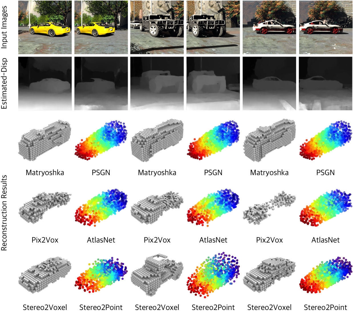
Figure 6: Reconstruction results compared to the state-of-the-arts methods on the Driving dataset. Estimated-Disp represents the disparities estimated by DispNet-B. Note that PSGN takes object masks as an additional input.

To evaluate the performance of the proposed methods in handling naturalistic images, we compare our methods against Matryoshka, Pix2Vox, PSGN, and AltasNet on a subset of the Driving dataset (?). We fine-tune all methods on the car category of the StereoShapeNet dataset using backgrounds that are randomly sampled from the SUN database (?). We further augment our training data by random color and light jittering. For better generalize to naturalistic scenarios, we pretrain DispNet-B on the FlyingThings 3D dataset (?).

For testing, we select several untruncated and unoccluded car images in the Driving dataset. First, the images are cropped according to the bounding box of the largest cars within the image. Then, these cropped images are rescaled to the input size of the networks. Figure 6 shows some representative reconstruction results of Stereo2Voxel and Stereo2Point compared with other methods on the Driving dataset. Except for Pix2Vox, all competitive methods produce almost the same reconstruction results for the three images, which indicates that single-view reconstruction methods rarely reason about the 3D structure of an object and tend to output a mean shape to minimize the reconstruction errors. In contrast, Stereo2Voxel and Stereo2Point recovers better skeletons of objects than other methods.

Ablation Study

Table 2: The ablation studies of DispNet-B and CorrNet. Intersection over union (IoU) and Chamfer distance (CD) are adopted to evaluate the performance for Stereo2Voxel and Stereo2Point, respectively. Note that the CD is computed on 1024 points and multiplied by $10^{3}$.

DispNet-B	CorrNet	Stereo2Voxel	Stereo2Point
✓	✓	0.702	1.185
✓	$\times$	0.690	1.284
$\times$	✓	0.678	1.379
$\times$	$\times$	0.651	1.570

Table 3: The comparison of the numbers of parameters, inference times, and the endpoint error (EPE) on the StereoShapeNet and the subset of FlyingThings 3D and dataset. Note that the inference time is for a 960$\times$540 image on an NVIDIA GTX 1080 Ti GPU.

Methods	DispNet-B	DispNet	GA-Net
#Parameters (M)	2.54	39.45	6.58
Inference Time (s)	0.018/pair	0.063	6.999
FlyingThings 3D (EPE)	1.292	1.157	0.515
StereoShapeNet (EPE)	0.096	0.092	0.089

Table 4: The comparison of reconstruction results with different disparity map quality on the StereoShapeNet dataset. Intersection over union (IoU) and Chamfer distance (CD) are adopted to evaluate the performance for Stereo2Voxel and Stereo2Point, respectively. Note that the CD is computed on 1024 points and multiplied by $10^{3}$.

Methods	Stereo2Voxel	Stereo2Point
SGBM	0.680	1.282
DispNet-B	0.702	1.185
DispNet	0.702	1.184
GA-Net	0.705	1.178

In this section, we validate the effectiveness of two key components of our method: DispNet-B and CorrNet.

DispNet-B. Both Stereo2Voxel and Stereo2Point estimate the disparity maps from a pair of stereo images. To demonstrate the importance of disparities in stereo 3D reconstruction, we remove DispNet-B from the proposed methods. The stereo RGB images are directly fed into the encoders in RecNet without estimating disparities. As illustrated in Table 2, removing DispNet-B causes an increase of $16.4\%$ in CD for Stereo2Points. The IoU decreases to $0.678$ when removing DispNet-B from Stereo2Voxel.

CorrNet. CorrNet aims to find feature correspondences between a pair of stereo images. To quantitatively evaluate CorrNet, we compare the performance of Stereo2Voxel and Stereo2Point without CorrNet. As shown in Table 2, the CD increases to $1.284$ when CorrNet is removed from Stereo2Points. The IoU decreases to $0.690$ when removing CorrNet from Stereo2Voxel. Moreover, removing both DispNet-B and CorrNet results in worse reconstruction results in both Stereo2Point and Stereo2Voxel, where the CD increases by $32.5\%$ in Stereo2Point and the IoU decreases by $7.3\%$ in Stereo2Voxel, respectively.

Discussion

Performance Evaluation of DispNet-B. To further compare DispNet-B with other stereo matching methods, we evaluate the performance of DispNet-B on the subset of Flying Things 3D (clean pass, disparity $<$ 96 pixels) test dataset. Since we only care about the results of predicted disparity in non-occluded regions, we adopt the endpoint error (EPE) on non-occluded regions as the measure. As shown in Table 3, the EPE of DispNet-B is comparable with DispNet (?) and worse than GA-Net (?). However, DispNet-B is only 6% size of DispNet and 38% size of GA-Net. In terms of inferring time, DispNet-B is about 7 and 778 times faster than DispNet and GA-Net, respectively. Moreover, DispNet-B can predict the bidirectional disparity maps for both views simultaneously.

Effectiveness of Disparity Map Quality. To quantitatively compare the reconstruction results of Stereo2Voxel and Stereo2Points with different disparities, we replace DispNet-B with SGBM (?), DispNet, and GA-Net. As shown in Table 4, the reconstruction results with disparities estimated by DispNet and GA-Net are slightly better than with disparities estimated by DispNet-B, while SGBM degenerates the reconstruction results. The experimental results indicate that better disparities lead to better reconstruction results.

Conclusion

In this paper, we present a novel framework to recover the 3D shape of an object from a pair of stereo images. The proposed method reasons about the 3D structure by exploring bidirectional disparities and feature corresponding between the two views. To our best knowledge, our work is the first to study 3D reconstruction from stereo images with deep learning. In order to support this work and inspire more studies towards this new direction, we also construct a large-scale synthetic dataset, named StereoShapeNet, which contains 1M pairs of stereo images rendered from ShapeNet along with the corresponding bidirectional depth and disparity maps. Quantitative and qualitative evaluation for both 3D volumes and point clouds on StereoShapeNet indicate that the proposed method outperforms state-of-the-art methods.

Acknowledgements This work was supported by the National Natural Science Foundation of China under Project No. 61772158, 61702136, 61872112 and U1711265.

References

- [Aloimonos 1988] Aloimonos, J. 1988. Shape from texture. Biological cybernetics 58(5):345–360.
- [Baker and Matthews 2004] Baker, S., and Matthews, I. A. 2004. Lucas-kanade 20 years on: A unifying framework. International Journal of Computer Vision 56(3):221–255.
- [Bhoi 2019] Bhoi, A. 2019. Monocular depth estimation: A survey. arXiv 1901.09402.
- [Buelthoff and Yuille 1991] Buelthoff, H. H., and Yuille, A. L. 1991. Shape-from-x: Psychophysics and computation. In Sensor Fusion III: 3D Perception and Recognition, volume 1383, 235–247. International Society for Optics and Photonics.
- [Chen et al. 2018] Chen, Y.; Ren, J.; Cheng, X.; Qian, K.; and Gu, J. 2018. Very power efficient neural time-of-flight. arXiv 1812.08125.
- [Choy et al. 2016] Choy, C. B.; Xu, D.; Gwak, J.; Chen, K.; and Savarese, S. 2016. 3D-R2N2: A unified approach for single and multi-view 3D object reconstruction. In ECCV 2016.
- [Chung et al. 2014] Chung, J.; Gülçehre, Ç.; Cho, K.; and Bengio, Y. 2014. Empirical evaluation of gated recurrent neural networks on sequence modeling. In NIPS Workshops 2014.
- [Fan, Su, and Guibas 2017] Fan, H.; Su, H.; and Guibas, L. J. 2017. A point set generation network for 3D object reconstruction from a single image. In CVPR 2017.
- [Groueix et al. 2018] Groueix, T.; Fisher, M.; Kim, V. G.; Russell, B. C.; and Aubry, M. 2018. A papier-mâché approach to learning 3D surface generation. In CVPR 2018.
- [He et al. 2016] He, K.; Zhang, X.; Ren, S.; and Sun, J. 2016. Deep residual learning for image recognition. In CVPR 2016.
- [Hirschmuller 2007] Hirschmuller, H. 2007. Stereo processing by semiglobal matching and mutual information. TPAMI 30(2):328–341.
- [Iandola et al. 2017] Iandola, F. N.; Moskewicz, M. W.; Ashraf, K.; Han, S.; Dally, W. J.; and Keutzer, K. 2017. Squeezenet: Alexnet-level accuracy with 50x fewer parameters and <1mb model size. In ICLR 2017.
- [Ilg et al. 2018] Ilg, E.; Saikia, T.; Keuper, M.; and Brox, T. 2018. Occlusions, motion and depth boundaries with a generic network for disparity, optical flow or scene flow estimation. In ECCV 2018.
- [Kar, Häne, and Malik 2017] Kar, A.; Häne, C.; and Malik, J. 2017. Learning a multi-view stereo machine. In NIPS 2017.
- [Kendall et al. 2017] Kendall, A.; Martirosyan, H.; Dasgupta, S.; and Henry, P. 2017. End-to-end learning of geometry and context for deep stereo regression. In ICCV 2017.
- [Kingma and Ba 2015] Kingma, D. P., and Ba, J. 2015. Adam: A method for stochastic optimization. In ICLR 2015.
- [Li et al. 2017] Li, D.; Shao, T.; Wu, H.; and Zhou, K. 2017. Shape completion from a single RGBD image. IEEE Trans. Vis. Comput. Graph. 23(7):1809–1822.
- [Mayer et al. 2016] Mayer, N.; Ilg, E.; Häusser, P.; Fischer, P.; Cremers, D.; Dosovitskiy, A.; and Brox, T. 2016. A large dataset to train convolutional networks for disparity, optical flow, and scene flow estimation. In CVPR 2016.
- [Nealen et al. 2006] Nealen, A.; Igarashi, T.; Sorkine, O.; and Alexa, M. 2006. Laplacian mesh optimization. In SIGGRAPH 2006.
- [Newcombe, Lovegrove, and Davison 2011] Newcombe, R. A.; Lovegrove, S.; and Davison, A. J. 2011. DTAM: dense tracking and mapping in real-time. In ICCV 2011.
- [Richter and Roth 2018] Richter, S. R., and Roth, S. 2018. Matryoshka networks: Predicting 3d geometry via nested shape layers. In CVPR 2018.
- [Tatarchenko et al. 2019] Tatarchenko, M.; Richter, S. R.; Ranftl, R.; Li, Z.; Koltun, V.; and Brox, T. 2019. What do single-view 3D reconstruction networks learn? In CVPR 2019.
- [Tatarchenko, Dosovitskiy, and Brox 2017] Tatarchenko, M.; Dosovitskiy, A.; and Brox, T. 2017. Octree generating networks: Efficient convolutional architectures for high-resolution 3D outputs. In ICCV 2017.
- [Wu et al. 2015] Wu, Z.; Song, S.; Khosla, A.; Yu, F.; Zhang, L.; Tang, X.; and Xiao, J. 2015. 3D ShapeNets: A deep representation for volumetric shapes. In CVPR 2015.
- [Wu et al. 2017] Wu, J.; Wang, Y.; Xue, T.; Sun, X.; Freeman, B.; and Tenenbaum, J. 2017. MarrNet: 3D shape reconstruction via 2.5D sketches. In NIPS 2017.
- [Xiao et al. 2010] Xiao, J.; Hays, J.; Ehinger, K. A.; Oliva, A.; and Torralba, A. 2010. SUN database: Large-scale scene recognition from abbey to zoo. In CVPR 2010.
- [Xie et al. 2019] Xie, H.; Yao, H.; Sun, X.; Zhou, S.; and Zhang, S. 2019. Pix2Vox: Context-aware 3D reconstruction from single and multi-view images. In ICCV 2019.
- [Yang et al. 2018] Yang, B.; Rosa, S.; Markham, A.; Trigoni, N.; and Wen, H. 2018. Dense 3D object reconstruction from a single depth view. TPAMI DOI: 10.1109/TPAMI.2018.2868195.
- [Zhang et al. 2018] Zhang, X.; Zhang, Z.; Zhang, C.; Tenenbaum, J.; Freeman, B.; and Wu, J. 2018. Learning to reconstruct shapes from unseen classes. In NeurIPS 2018.
- [Zhang et al. 2019] Zhang, F.; Prisacariu, V. A.; Yang, R.; and Torr, P. H. S. 2019. Ga-net: Guided aggregation net for end-to-end stereo matching. In CVPR 2019.
- [Zhao, Gao, and Lin 2007] Zhao, W.; Gao, S.; and Lin, H. 2007. A robust hole-filling algorithm for triangular mesh. The Visual Computer 23(12):987–997.