Improving the convergence of SGD through adaptive batch sizes

Abstract

Mini-batch stochastic gradient descent (SGD) and variants thereof approximate the objective function’s gradient with a small number of training examples, aka the batch size. Small batch sizes require little computation for each model update but can yield high-variance gradient estimates, which poses some challenges for optimization. Conversely, large batches require more computation but can yield higher precision gradient estimates. This work presents a method to adapt the batch size to the model’s training loss. For various function classes, we show that our method requires the same order of model updates as gradient descent while requiring the same order of gradient computations as SGD. This method requires evaluating the model’s loss on the entire dataset every model update. However, the required computation is greatly reduced by approximating the training loss. We provide experiments that illustrate our methods require fewer model updates without increasing the total amount of computation.

1 Introduction

Mini-batch SGD and variants thereof Bottou et al. (2018) are extremely popular in machine learning (e.g., Zou et al. (2017); Szegedy et al. (2017); Simon et al. (2016)). These methods attempt to minimize a function $F(\bm{w}):=\nicefrac{{1}}{{n}}\sum_{i=1}^{n}f(\bm{w};\bm{z}_{i})$ where the function $f$ measures the loss of a model $\bm{w}$ on example $\bm{z}_{i}$. For example, if performing linear regression on $d$ features, $\bm{z}_{i}=(\bm{x}_{i},y_{i})$ which includes a feature vector $\bm{x}_{i}\in\mathbb{R}^{d}$ and scalar output variable $y_{i}\in\mathbb{R}$. To minimize $F$, mini-batch SGD uses $B$ examples to compute a model update via

$$\bm{w}_{k+1}=\bm{w}_{k}-\frac{\gamma_{k}}{B}\sum_{i=1}^{B}\nabla f(\bm{w}_{k};\bm{z}_{i_{s}})$$ (1)

where $\gamma_{k}$ is the step-size or learning rate at model update $k$ and $i_{s}$ is chosen uniformly at random. This update approximates $F$’s gradient with $B$ examples in order to make the complexity of each model update scale with $B$, typically much smaller than $n$ Bottou (2012).

In practice, the batch size $B$ is a hyper-parameter and is often constant throughout the optimization (e.g, Alistarh et al. (2017); Zagoruyko and Komodakis (2016); Goyal et al. (2017)). There is a clear tradeoff between small and large batch sizes for each model update: using small batch sizes reduces the computation required for each model update while yielding imprecise estimates of the objective function’s gradient. Conversely, large batch sizes yield more precise gradient estimates, but fewer model updates can be performed with the same computation budget.

1.1 Contributions

Why should the batch size remain static as an optimization proceeds? With poor initialization, the optimal model for each example is in the same direction. In this case, approximating the objective function’s gradient with more examples will have little benefit because each gradient is similar. By that measure, perhaps large batch sizes will provide utility near the optimum because the optimum depends on all training examples.

This work expands upon the idea by adaptively growing the batch size with model performance as the optimization proceeds. Specifically, this work does the following:

• Provides methods to adapt the batch size to the model performance. These methods require significant computation because they require computing model performance before every model update.

• Shows that adapting the batch size to the model performance can require significantly fewer model updates and approximately the same number of gradient computations when compared with standard SGD.

• Provides a practical implementation that circumvents the requirement to evaluate the objective function before every model update.

• Provides experimental results on both methods. These experiments show that the methods above require fewer model updates and the same number of gradient computations as standard mini-batch SGD to reach a particular accuracy.

The benefit of reducing the number of model updates isn’t apparent at first glance. One benefit is that the wall-clock time required for any one model update is agnostic to the batch size with a certain distributed system configuration (Goyal et al., 2017, Sec. 5.5). When the batch size grows geometrically, the number of model updates is a “meaningful measure of the training time” in a similar system (Smith et al., 2018, Sec. 5.4). Additionally, larger batch sizes improve distributed system performance Qi et al. (2016); Yin et al. (2018).

Our adaptive method receives the function value in addition to the gradients, which is more information than SGD and variants thereof receive Nemirovsky and Yudin (1983). However, in practice, our proposed practical implementation largely ignores the gradient norm and essentially only receives the function value.

In Section 3, some preliminary notions are introduced before the presentation of the adaptive batch size method and the corresponding convergence results in Section 4. We address some practical implementation issues and provide validating experiments in Section 5.

2 Related work

Mini-batch SGD with small batch sizes tends to bounce around the optimum because the gradient estimate has high variance – the optimum depends on all examples, not a few examples. Common methods to circumvent this issue include some step size decay schedule (Bottou, 1998, Sec. 4) and averaging model iterates with averaged SGD (ASGD) Polyak and Juditsky (1992). Less common methods include stochastic average gradient (SAG) and stochastic variance reduction (SVRG) because they present memory and computational restrictions respectively Schmidt et al. (2013); Johnson and Zhang (2013). Our work is more similar in spirit to variance reduction techniques that use variable learning rates and batch sizes, discussed below.

Adaptive learning rates

Adaptive learning rates or step sizes can help adapt the optimization to the most informative features with Adagrad Ward et al. (2019); Duchi et al. (2011) or to estimate the first and second moments of the gradients with Adam Kingma and Ba (2014). Adagrad has inspired Adadelta Zeiler (2012) which makes some modifications to average over a certain window and approximate the Hessian. Such methods are useful for convergence and a reduction in hyperparameter tuning. AdaGrad and variants thereof give principled, robust ways to vary the learning rate that avoid having to tune learning rate decay schedules Ward et al. (2019).

Increasing batch sizes

Increasing the batch size as an optimization proceeds is another method of variance reduction. Strongly convex functions provably benefit from geometrically increasing batch sizes in terms of the number of model updates while requiring no more gradient computations than SGD (Bottou et al., 2018, Ch. 5). The number of model updates required for strongly convex, convex and non-convex functions is improved with batch sizes that increase like $\mathcal{O}\left(r^{k}\right)$, $\mathcal{O}\left(k^{2}\right)$ and $\mathcal{O}\left(k\right)$ respectively Zhou et al. (2018).

Smith et al. perform variance reduction by geometrically increasing the batch size or decreasing the learning rate by the same factor, both in discrete steps (e.g., every 60 epochs) Smith et al. (2018). Specifically, Smith et al. motivate their method by connecting variance reduction to simulated annealing, in which reducing the SGD model update variance or “noise scale” in a series of discrete steps enhances the likelihood of reaching a “robust” minima (Smith et al., 2018, Sec. 3).

Smith et al. show that increasing the batch size yields similar results to decaying the learning rate by the same amount, which suggests that “it is the noise scale which is relevant, not the learning rate” (Smith et al., 2018, Sec. 5.1). By that measure, adaptive batch sizes are to geometrically increasing batch sizes as adaptive learning rate methods are to SGD learning rate decay schedules.

Adaptive batch sizes

Several schemes to adapt the batch size to the model have been developed, ranging from model specific schemes Orr (1997) to more general schemes De et al. (2016); Balles et al. (2017); Byrd et al. (2012). These methods tend to look at the sample variance of every individual gradient, which involves the computation of a single gradient norm $\left\lVert\nabla f_{i}(\bm{x})\right\rVert$ for every example $i$ in the current batch Byrd et al. (2012); Balles et al. (2017); De et al. (2016). Naively, this requires feeding every example through the model individually. This can be circumvented; Balles et al. present an approximation method to avoid the variance estimation that requires about $1.25\times$ more computation than the standard mini-batch SGD update, with some techniques to avoid memory constraints (Balles et al., 2017, Sec. 4.2).

Friedlander et al. use adaptive batch sizes to prove linear convergence for strongly convex functions and a $\mathcal{O}\left(1/k\right)$ convergence rate for convex functions Friedlander and Schmidt (2012). Their adaptive approach relies on providing a batch size that satisfies certain error bounds on the gradient residual (in Eq. 2.6), which provides motivation for geometrically increasing batch sizes (Friedlander and Schmidt, 2012, Sec. 3).

Work developed concurrently with this work includes an SVRG modification Ji et al. (2019), which involves modifying the outer-loop of SVRG. Instead of calculating the gradient for all $n$ examples during every loop, they propose a scheme to calculate the gradient for $N_{s}$ examples where $N_{s}$ is inversely proportional to the average gradient variance.

3 Preliminaries

First, some basic definitions:

Definition 1.

A function $F$ is $L$-Lipschitz if $\left\lVert F(\bm{w}_{1})-F(\bm{w}_{2})\right\rVert\leq L\left\lVert\bm{w}_{1}-\bm{w}_{2}\right\rVert~{}\forall~{}\bm{w}_{1},\bm{w}_{2}$.

Definition 2.

A function $F$ is $\beta$-smooth if the gradients are $\beta$-Lipschitz, or if $\left\lVert\nabla F(\bm{w}_{1})-\nabla F(\bm{w}_{2})\right\rVert\leq\beta\left\lVert\bm{w}_{1}-\bm{w}_{2}\right\rVert~{}\forall\bm{w}_{1},\bm{w}_{2}$.

The class of $\beta$-smooth functions is a result of the gradient norm being bounded, or that all the eigenvalues of the Hessian are smaller than $\beta$. If a function $F$ is $\beta$-smooth, the function also obeys $\forall x_{1},x_{2},~{}F(\bm{w}_{1})\leq F(\bm{w}_{2})+\left<\nabla F(\bm{w}_{2}),\bm{w}_{1}-\bm{w}_{2}\right>+\frac{\beta}{2}\left\lVert\bm{w}_{1}-\bm{w}_{2}\right\rVert_{2}^{2}$ (Bubeck et al., 2015, Lemma 3.4).

Definition 3.

A function $F$ is $\alpha$-strongly convex if $\forall\bm{w}_{1},\bm{w}_{2},~{}F(\bm{w}_{1})\geq F(\bm{w}_{2})+\left<\nabla F(\bm{w}_{2}),\bm{w}_{1}-\bm{w}_{2}\right>+\frac{\alpha}{2}\left\lVert\bm{w}_{1}-\bm{w}_{2}\right\rVert_{2}^{2}$.

$\alpha$-strongly convex functions grow quadratically away from the optimum $\bm{w}^{\star}=\arg\min_{\bm{w}}F(\bm{w})$ since $F(\bm{w})-F(\bm{w}^{\star})\geq\frac{\alpha}{2}\left\lVert\bm{w}-\bm{w}^{\star}\right\rVert^{2}_{2}$. While amenable to analysis, this criterion is often too restrictive. The Polyak- Łojasiewicz condition is a generalization of strong convexity that’s less restrictive Polyak (1963); Karimi et al. (2016):

Definition 4.

A function $F$ obeys Polyak-Łojasiewicz (PL) condition with parameter $\alpha>0$ if $\frac{1}{2}\left\lVert\nabla F(\bm{w})\right\rVert_{2}^{2}\geq\alpha(F(\bm{w})-F^{\star})$ when $F^{\star}=\min_{\bm{w}}F(\bm{w})$.

For simplicity, we refer to these functions $F$ satisfying this condition as being “$\alpha$-PL.” The class of $\alpha$-PL functions includes $\alpha$-strongly convex functions and a certain class non-convex functions Karimi et al. (2016). One important constraint of $\alpha$-PL functions is that every stationary point must be a global minimizer, though stationary points are not necessarily unique. Recent work has shown similar convergence rates for $\alpha$-PL and $\alpha$-strongly convex functions for a variety of different algorithms Karimi et al. (2016).

A bound on the expected gradient norm will also be useful because it will appear in theorem statements. For ease of notation, let’s define $f_{i}(\bm{w}):=f(\bm{w};\bm{z}_{i})$.

Definition 5.

For model $\bm{w}$, let $M^{2}(\bm{w}):=\nicefrac{{1}}{{n}}\sum_{i=1}^{n}\left\lVert\nabla f_{i}(\bm{w})\right\rVert_{2}^{2}$ and let $\mathcal{M}:=\{M^{2}(\bm{w}_{k}):k\in\mathbb{N}\cup\{0\}\text{ and }k<T\}$ when $T$ model updates are performed. Let $M^{2}_{L}:=\min\mathcal{M}$ and $M^{2}_{U}:=\max\mathcal{M}$.

4 Convergence

In this section we will prove convergence rates for mini-batch SGD with adaptive batch sizes and give bounds on the number of gradient computations needed. Our main results are summarized in Table 0(b). In general, this work shows that mini-batch SGD with appropriately chosen adaptive batch sizes requires the same number of model updates as gradient descent (up to constants) while not requiring more gradient computations than serial SGD (up to constants).

In general, the adaptive batch sizes are inversely proportional to the current model’s loss. This method is motivated by an approximate measure of gradient dissimilarity as detailed in Appendix A. Section 4.1 analyzes the required number of model updates, and Section 4.2 analyzes the required number of gradient computations. The theory in this section might require significant computation; methods in Section 5 circumvent some of these issues.

Table 1: The number of model updates or gradient computations required to reach a model of error at most $\varepsilon$. Error is defined with loss $F(\bm{w}_{T})-F^{\star}\leq\varepsilon$ for smooth & convex functions and $\alpha$-strongly convex ($\alpha$-SC) functions, and with gradient norm for smooth functions, $\min_{k=0,\ldots,T-1}\left\lVert\nabla F(\bm{w}_{k})\right\rVert\leq\varepsilon$. All function classes are $\beta$-smooth, and for $\alpha$-strongly convex functions the condition number $\kappa$ is given by $\kappa=\beta/\alpha$. The function class column in Table 0(a) is shared with Table 0(b). See Section 4 for details and references. Cells with minimum model updates/gradient computations (up to constants) with $n=60\cdot 10^{3}$, $\varepsilon=0.01$, $\alpha=0.1$ and $\beta=1$ are highlighted.

Function	SGD	Adaptive	Gradient
class		batch sizes	descent
$\alpha$-SC	$\mathcal{O}\left(\nicefrac{{\kappa}}{{\beta\varepsilon}}\right)$	$\mathcal{O}\left(\kappa\log(\nicefrac{{1}}{{\varepsilon}})\right)$	$\mathcal{O}\left(\kappa\log(\nicefrac{{1}}{{\varepsilon}})\right)$
Convex	$\mathcal{O}\left(\nicefrac{{1}}{{\varepsilon^{2}}}\right)$	$\mathcal{O}\left(\nicefrac{{1}}{{\varepsilon}}\right)$	$\mathcal{O}\left(\nicefrac{{1}}{{\varepsilon}}\right)$
Smooth	$\mathcal{O}\left(\nicefrac{{1}}{{\varepsilon^{4}}}\right)$	$\mathcal{O}\left(\nicefrac{{1}}{{\varepsilon^{2}}}\right)$	$\mathcal{O}\left(\nicefrac{{1}}{{\varepsilon^{2}}}\right)$

(a) Total number of model updates required during optimization.

SGD	Adaptive	Gradient
	batch sizes	descent
$\mathcal{O}\left(\nicefrac{{\kappa}}{{\beta\varepsilon}}\right)$	$\mathcal{O}\left(\nicefrac{{\kappa}}{{\varepsilon}}\log(\nicefrac{{1}}{{\varepsilon}}\right))$	$\mathcal{O}\left(n\kappa\log(\nicefrac{{1}}{{\varepsilon}}\right))$
$\mathcal{O}\left(\nicefrac{{1}}{{\varepsilon^{2}}}\right)$	$\mathcal{O}\left(\nicefrac{{1}}{{\varepsilon^{2}}}\right)$	$\mathcal{O}\left(\nicefrac{{n}}{{\varepsilon}}\right)$
$\mathcal{O}\left(\nicefrac{{1}}{{\varepsilon^{4}}}\right)$	$\mathcal{O}\left(\nicefrac{{1}}{{\varepsilon^{3}}}\right)$	$\mathcal{O}\left(\nicefrac{{n}}{{\varepsilon^{2}}}\right)$

(b) Total number of gradient computations required during optimization.

4.1 Model updates

Let’s start in the context of $\alpha$-PL functions. In this setting, SGD requires $\mathcal{O}\left(\nicefrac{{1}}{{\varepsilon}}\right)$ model updates (Karimi et al., 2016, Thm. 4). Gradient descent with a constant learning rate requires $\log\left(\nicefrac{{1}}{{\varepsilon}}\right)$ model updates (Karimi et al., 2016, Thm. 1), as does SGD with geometrically increasing batch sizes for strongly convex functions (Bottou et al., 2018, Cor. 5.2). We show that $\log{\left(\nicefrac{{1}}{{\varepsilon}}\right)}$ model updates are also required when the adaptive batch size is chosen appropriately:

Theorem 1.

Let $\bm{x}_{k}$ denote the $k$-th iterate of mini-batch SGD with step-size $\gamma$ on a $\beta$-smooth and $\alpha$-PL function $F$. If the batch size $B_{k}$ at each iteration $k$ is given by

$$B_{k}=\left\lceil\frac{c}{F(\bm{w}_{k})-F^{\star}}\right\rceil$$ (2)

and the learning rate $\gamma=\alpha/[\beta\left(\alpha+M^{2}_{U}/2c\right)]$ for some constant $c>0$, then

$$\mathbb{E}\left[F(\bm{w}_{T})\right]-F^{\star}\leq\left(1-r\right)^{T}(F(\bm{w}_{0})-F^{\star})$$

where $r\coloneqq\alpha^{2}/\left(\beta\left(\alpha+M^{2}_{U}/2c\right)\right)$. This implies $T\geq\mathcal{O}\left(\log{\left(\nicefrac{{1}}{{\varepsilon}}\right)}\right)$ model updates are required to obtain $\bm{w}_{T}$ such that $\mathbb{E}\left[F(\bm{w}_{T})\right]-F^{\star}\leq\varepsilon$.

The proof is detailed in Appendix B.1 and follows from the definition of $B_{k}$, $\beta$-smooth and $\alpha$-PL. This theorem can also be applied to Euclidean distance from the optimal model for $\alpha$-strongly convex functions because $\nicefrac{{\alpha}}{{2}}\left\lVert\bm{w}_{k}-\bm{w}^{\star}\right\rVert_{2}^{2}\leq F(\bm{w}_{k})-F(\bm{w}^{\star})$. The learning rate $\gamma$ is typically a user-specified hyperparameter determined through trial-and-error (e.g, Schaul et al. (2013); Smith (2015)). This theorem makes a fairly standard assumption that the optimal training loss $F^{\star}$ is known, which influences $\gamma$ in Ward et al. (2019, Sec. 1.1) and Orr (1997, Eq. 15).

When $F$ is convex, the same adaptive batch size method obtains comparable convergence rates to gradient descent. SGD requires $\mathcal{O}\left(\nicefrac{{1}}{{\varepsilon^{2}}}\right)$ model updates (Bubeck et al., 2015, Thm. 6.3). Gradient descent with constant learning rate requires $\mathcal{O}\left(\nicefrac{{1}}{{\varepsilon}}\right)$ model updates (Bubeck et al., 2015, Thm. 3.3), and has linear convergence if an exact line search is used (Boyd and Vandenberghe, 2004, Eq. 9.18). Using adaptive batch sizes with SGD also requires $\mathcal{O}\left(\nicefrac{{1}}{{\varepsilon}}\right)$ model updates:

Theorem 2.

Let $\bm{x}_{k}$ denote the $k$-th iterate of mini-batch SGD with step size $\gamma$ on some $\beta$-smooth and convex function $F$. If the batch size $B_{k}$ at each iteration is given by Equation 2 and $\gamma=(\beta+1/c)^{-1}$, then for any $T\geq 1$,

$$\mathbb{E}\left[F\left(\macc@depth\char 1\relax\frozen@everymath{\macc@group}\macc@set@skewchar\macc@nested@a 111{\bm{w}}_{T}\right)\right]-F^{\star}\leq\frac{r}{T}$$

where $r\coloneqq\|\bm{w}_{0}-\bm{w}^{*}\|^{2}\left(\beta+\frac{M_{U}^{2}}{c}\right)+F(\bm{w}_{0})-F^{*}$ and $\macc@depth\char 1\relax\frozen@everymath{\macc@group}\macc@set@skewchar\macc@nested@a 111{\bm{w}}_{T}:=\frac{1}{T}\sum_{i=0}^{T-1}\bm{w}_{i+1}$. This implies $T\geq\nicefrac{{r}}{{\varepsilon}}$ model updates are required to obtain $\bm{w}_{T}$ such that $\mathbb{E}\left[F(\bm{w}_{T})\right]-F^{\star}\leq\varepsilon$.

This proof adapts classic convergence analysis of SGD Bubeck et al. (2015) and is in Appendix B.2.

Key Lemma

Theorems 1 and 2 rely on a key lemma, one that controls the gradient approximation error $\mathbb{E}\left[\left\lVert\nabla F(\bm{w}_{k})-\bm{g}_{k}\right\rVert_{2}^{2}\right]$ as a function of the number of model updates $k$ and batch size $B_{k}$. When the batch size is grown according to Eq. 2, the gradient approximation error for model update $k$ is bounded by the loss of model $\bm{w}_{k}$:

Lemma 3.

Let the batch size $B_{k}$ be chosen as in Eq. 2. Then when the gradient estimate $\bm{g}_{k}=\nicefrac{{1}}{{B_{k}}}\sum_{i=1}^{B_{k}}\nabla f_{i_{s}}(\bm{w}_{k})$ is created with $i_{s}$ chosen uniformly at random, then

$$\mathbb{E}\left[\|\nabla F(\bm{w}_{k})-\bm{g}_{k}\|_{2}^{2}\>\Big{|}\>\bm{w}_{k}\right]\leq(F(\bm{w}_{k})-F^{\star})M_{U}^{2}c^{-1}$$

The proof is Appendix B and relies on substituting the definition of the batch size $B_{k}$ into the gradient approximation error, $\mathbb{E}\left[\left\lVert\nabla F(\bm{w}_{k})-\bm{g}_{k}\right\rVert_{2}^{2}\right]$.

When $F$ is smooth and non-convex, we’ll provide an upper bound on the number of model updates required to find an $\varepsilon$-approximate critical point so that $\left\lVert\nabla F(\bm{x})\right\rVert\leq\varepsilon$, which requires computing the adaptive batch size differently. In this setting, SGD requires $\mathcal{O}\left(\nicefrac{{1}}{{\varepsilon^{4}}}\right)$ model updates (Yin et al., 2018, Thm. 2), and gradient descent requires $\mathcal{O}\left(\nicefrac{{1}}{{\varepsilon^{2}}}\right)$ model updates (Jin et al., 2017, Thm. 2). Adaptive batch sizes require $\mathcal{O}\left(\nicefrac{{1}}{{\varepsilon^{2}}}\right)$ model updates:

Theorem 4.

Let $\bm{x}_{k}$ denote the $k$-th iterate of mini-batch SGD on a $\beta$-smooth function $F$. If the batch size $B_{k}$ at each iteration satisfies

$$B_{k}=\left\lceil\frac{c}{\left\lVert\nabla F(\bm{w}_{k})\right\rVert_{2}^{2}}\right\rceil$$ (3)

for some $c>0$ and the step size $\gamma=\beta^{-1}\cdot c/(c+M_{L}^{2})$, then for any $T\geq 1$,

$$\min_{k=0,\ldots,T-1}\left\lVert\nabla F(\bm{w}_{k})\right\rVert\leq\sqrt{\frac{r}{T}}$$

where $r\coloneqq 2(F(\bm{w}_{0})-F^{\star})\cdot\beta\left(M_{L}^{2}c^{-1}+1\right)$. This implies $T\geq\nicefrac{{r^{2}}}{{\varepsilon^{2}}}$ model updates are required to obtain $\bm{w}_{T}$ such that $\min_{k=0,\ldots,T-1}\left\lVert\nabla F(\bm{w}_{k})\right\rVert\leq\varepsilon$.

The proof adapts a proof by Yin et al. (2018, Thm. 2) to the batch size in Equation 3 and is detailed in Appendix B.3.

4.2 Number of gradient computations

While the convergence rates above show that adaptively chosen batch sizes can lead to fast convergence in terms of the number of model updates, this is not a good metric for the total amount of work performed. When the model is close to the optimum, the batch size will be large but only one model update will be computed. A better metric for the amount of work performed is on the number of gradient computations required to reach a model of a particular error.

The number of gradient computations required by the adaptive batch size method is similar to the number of gradient computations for SGD. The number of gradient computations for SGD and gradient descent are reflected in the model update count; SGD and gradient descent require computing $1$ and $n$ gradients per model update respectively. These values are concisely summarized in Table 0(b).

Let’s start with $\alpha$-PL and convex functions. When increasing the batch size geometrically for $\alpha$-strong convex functions, only $\mathcal{O}\left(\nicefrac{{1}}{{\varepsilon}}\right)$ gradient computations are required (Bottou et al., 2018, Thm. 5.3).

Corollary 5.

When $F$ is $\alpha$-PL, no more than $4cr\log\left(\nicefrac{{1}}{{\varepsilon}}\right)/\varepsilon$ gradient computations are required in Theorem 1 for $c$ and $r$ defined therein.

Corollary 6.

For convex and $\beta$-smooth functions $F$, no more than $4cr/\varepsilon^{2}$ gradient computations are required in Theorem 2 for $c$ and $r$ defined therein.

Now, let’s look at the gradient computations required for smooth functions. For illustration, let’s assume the batch size in Eq. 3 is given by an oracle and does not require any gradient computation.

Corollary 7.

For $\beta$-smooth functions $F$, no more than $4cr/\varepsilon^{3}$ gradient computations are required to estimate the loss function’s gradient in Theorem 4 for $c$ and $r$ therein.

Proof is delegated to Appendix C. Corollaries 5, 6 and 7 rely on Lemma 14, which is not tight. Tightening this bound requires finding lower bounds on model loss, a statement of the form $F(\bm{w}_{k})-F^{\star}\geq g(\varepsilon,k)$ for some function $g$. There are classical bounds of this sort for gradient descent (Nesterov, 2013, Thms. 2.1.7 and 2.1.13), and more recent lower bounds for SGD Nguyen et al. (2019). However, deriving a comprehensive understanding of lower bounds for mini-batch SGD remains an open problem.

5 Experimental results & Practical considerations

In this section, we first show that the theory above works as expected: far fewer model are required to obtain a model of a particular loss, and the total number of gradient computations is the same as standard mini-batch SGD. However, the implementation above is impractical: the batch size requires significant computation. We suggest some workarounds to address these practical issues, and provide experiments that compare the proposed method with relevant work.

In this section, two performance metrics are relevant: the number of gradient computations and model updates to reach a particular accuracy. These two metrics can be treated as proxies for energy and time respectively. A single gradient computation requires a fixed number of floating point operations, which requires a fixed amount of energy. As discussed in Section 1.1, the wall-clock time required to complete one model update can be (almost) agnostic to the batch size with certain distributed systems.

5.1 Synthetic simulations

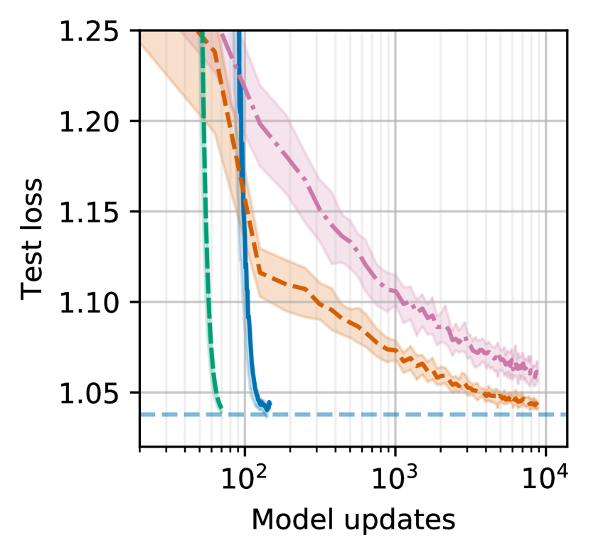
(a) The number of model updates required to reach a particular test accuracy.

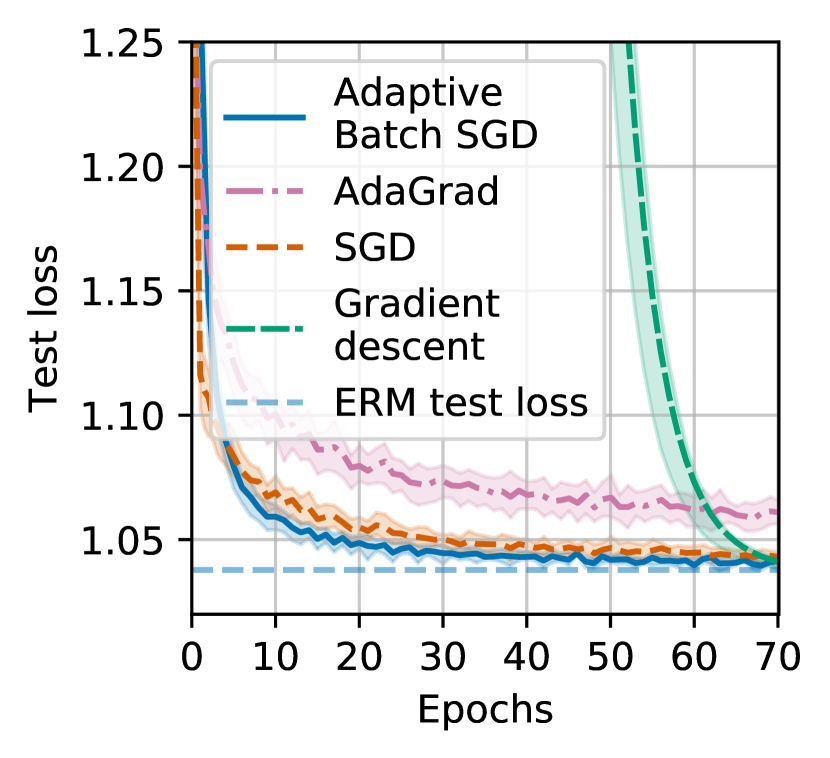
(b) The number of epochs required to be processed to reach a particular test accuracy.

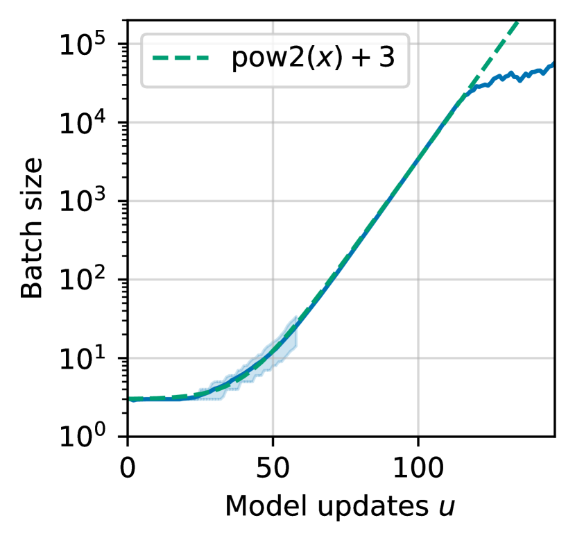
(c) The batch sizes and an exponential line. In the legend, $x=0.17(u-31)$ for $u$ model updates.

Figure 1: Different performance metrics for different optimizers for the minimization in Section 5.1. The legend in Figure 1(b) is shared with Figures 1(a) and 1(c), and the “ERM test loss” is the test loss of the linear ERM solution. “Epochs” refers to “$n$ training examples have been processed.” The solid lines represent the mean over 50 runs, and the shaded region represent the interquartile range.

First, let’s train a neural network with linear activations to illustrate our theoretical contributions. Practically speaking, this is an extremely inefficient and roundabout way to compute a linear function. However, the associated loss function is non-convex and more difficult to optimize. Despite the non-convexity it satisfies the PL inequality almost everywhere in a measure–theoretic sense (Charles and Papailiopoulos, 2018, Thm. 13). This section will focus on this optimization:

$$\widehat{\bm{w}}_{1},\widehat{\bm{W}}_{2},\widehat{\bm{W}}_{3}=\arg\min_{\bm{w}_{1},\bm{W}_{2},\bm{W}_{3}}\sum_{i=1}^{n}\left(y_{i}-\bm{w}_{1}^{T}\bm{W}_{2}\bm{W}_{3}\bm{x}_{i}\right)^{2}$$ (4)

where there are $n=10^{4}$ observations and each feature vector has $d=100$ dimensions, and $\bm{w}_{1}\in\mathbb{R}^{d}$, $\bm{W}_{2},\bm{W}_{3}\in\mathbb{R}^{d,d}$. The synthetic data $\bm{x}_{i}$ is generated with coordinates drawn independently from $\mathcal{N}(0,1)$. Each label $y_{i}$ is given by $y_{i}=\bm{x}_{i}^{T}\bm{w}^{\star}+n_{i}$ where $n_{i}\sim\mathcal{N}(0,\nicefrac{{d}}{{100}})$ and $\bm{w}^{\star}_{i}\sim\mathcal{N}(0,1)$. Of the $n=10^{4}$ observations, $2,000$ observations are used as test data.

In order to understand our adaptive batch size method, we compare the model updates in Theorem 1 (aka “Adaptive Batch SGD”) with mini-batch SGD to standard mini-batch SGD with decaying step size (SGD), gradient descent and Adagrad. The hyperparameters for these optimizers are not tuned and details are in Appendix D. Adagrad and SGD are run with batch size $B=64$.

Figure 1 shows that Adaptive Batch SGD requires far fewer model updates, not far from the number that gradient descent requires. Adaptive Batch SGD and SGD require nearly the same number of data, with Adagrad requiring more data than SGD but far less than gradient descent. Figure 1(c) shows that the batch size grows nearly exponentially, which unsurprising given Bottou et al. (2018, Eq. 5.7).

5.2 Functional implementation

Algorithm 1 RadaDamp(step size $\gamma$, memory $\rho=0.999$, initial batch size $B_{0}$, maximum batch size $B_{\max}$, initial model $\bm{w}_{0}$, regularization $\lambda=10^{-3})$

,

1:  for $k\in[0,1,2,\ldots]$ do

2:     $\gamma^{\prime}\leftarrow\gamma$

3:     if $B_{k}\geq B_{\max}$ then

4:        $\gamma^{\prime}\leftarrow\gamma B_{\max}/B_{k}$

5:        $B_{k}\leftarrow B_{\max}$

6:     end if

7:     $\widehat{L}_{B}\leftarrow\nicefrac{{1}}{{B_{k}}}\sum_{i=1}^{B_{k}}f_{i_{s}}(\bm{w}_{k})$

8:     $\bm{w}_{k+1}\leftarrow\bm{w}_{k}-\gamma^{\prime}\nabla\widehat{L}_{B}$

9:     $t_{k}\leftarrow\widehat{L}_{B}+\lambda\left\lVert\nabla\widehat{L}_{B}\right\rVert_{2}^{2}$

10:     if $k>0$ then

11:        $\widehat{d}_{k}\leftarrow\rho\cdot\widehat{d}_{k-1}+(1-\rho)t_{k}$

12:     else

13:        $\widehat{d}_{0}\leftarrow t_{k}$

14:     end if

15:     $B_{k+1}\leftarrow\left\lceil B_{0}\widehat{d}_{0}/\widehat{d}_{k}\right\rceil$

16:  end for

17:  return  $\bm{w}_{k+1}$

A practical issue immediately presents itself: the computation of the batch size $B_{k}$. This is clearly infeasible because it requires evaluating the entire training dataset every model update. To work around this issue, let’s approximate the training loss with a rolling-average of batch losses. Additionally, generalization and GPU memory concerns may be present. To address these concerns, prior work sets a maximum batch size and decays the learning rate by the same amount the batch size would have increased Smith et al. (2018); Devarakonda et al. (2017). Both actions reduces the “noise scale” or variance of the model update, and the results in Smith et al. (2018) “suggest that it is the noise scale which is relevant, not the learning rate.” This additional noise decay might help with generalization escape “sharp minima” that generalize poorly Smith and Le (2018); Keskar et al. (2016); Chaudhari et al. (2016)

The implementation of this algorithm is shown shown in Algorithm 1, which uses a rolling average to adaptively damp the noise in the gradient estimate. This algorithm is designed with these experiments in mind, the reason the batch size is inversely proportional to a linear combination of the training loss and gradient norm.

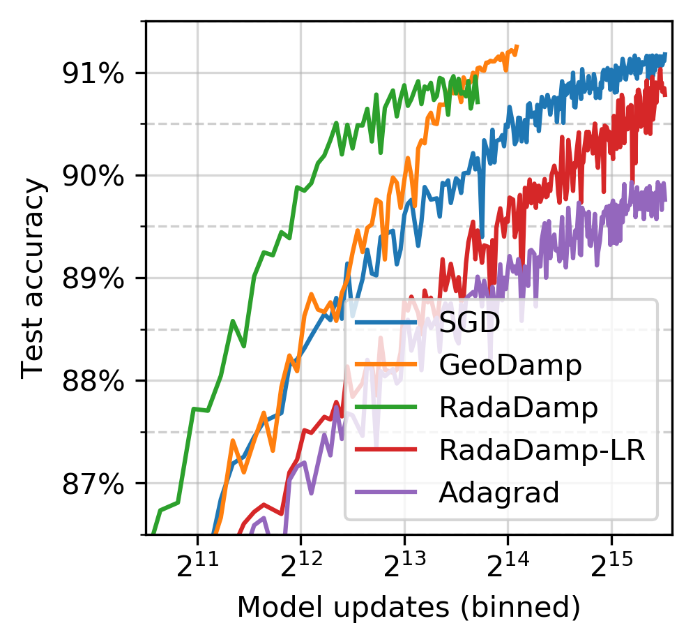
(a) The number of model updates vs. test accuracy.

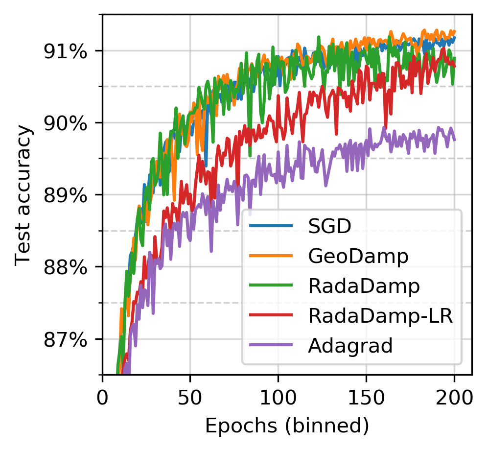
(b) The number of epochs vs. test accuracy.

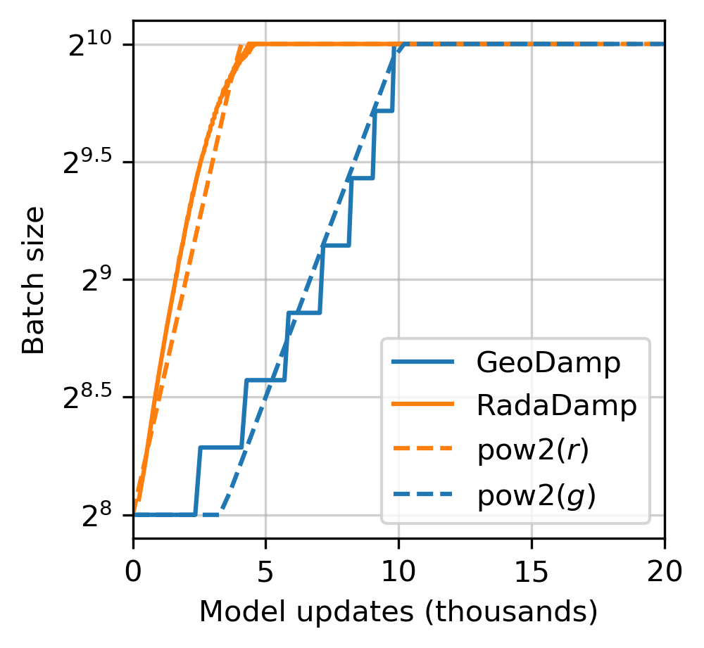
(c) The batch size against the number of model updates $u$. Here, $r=0.5u/10^{3}+8$ and
$g=0.3u/10^{3}+7$.

Figure 2: Performance on the Fashion-MNIST dataset. “Binned epochs” means “rounded to nearest integer” and “binned model updates” means “rounded to nearest multiple of 200.” The mean of these grouped values is used over the same two random seeds.

To evaluate our method, let’s use a convolutional neural network on the Fashion-MNIST dataset Xiao et al. (2017) with optimization algorithms that either passively or adaptively change the learning rate or batch size. Specifically, let’s compare RadaDamp with SGD, “GeoDamp” Smith et al. (2018), and AdaGrad Duchi et al. (2011). During this, let’s tune the batch size increase schedule for RadaDamp/GeoDamp, and use the same schedule for the corresponding algorithms that only decay the learning rate (“RadaDamp-LR” and SGD respectively). Details are in Appendix D.

	Final test
Optimizer	accuracy
GeoDamp	91.21%
SGD	91.11%
RadaDamp-LR	90.87%
RadaDamp	90.79%
Adagrad	89.83%

Figure 3: The mean test accuracy of the last 10 epochs.

Our experimental results are shown in Figure 2, details of which are in Appendix D. As expected, they show that RadaDamp and GeoDamp require far fewer model updates than RadaDamp-LR and SGD, and similar performance is obtained for all methods in terms of epochs. If the “noise scale” of the model updates is relevant as Smith et al. hypothesize Smith et al. (2018), then perhaps the relevant comparison is between passive and adaptive methods of changing the “noise scale” (i.e., RadaDamp is to Adagrad as GeoDamp is to SGD).

RadaDamp requires far fewer model updates than GeoDamp to reach any test accuracy RadaDamp obtains (though GeoDamp obtains a final test accuracy that is approximately 0.4% higher). Of course, Both Adagrad and RadaDamp require far less tuning than GeoDamp and SGD because of the adaptivity to the (estimated) training loss.

Figure 2(c) shows that both RadaDamp and GeoDamp (approximately) increase the batch size exponentially as functions of model updates, at least initially. However GeoDamp’s learning rate decays much more and far quicker than RadaDamp’s (perhaps a reason for GeoDamp’s increased performance).

6 Conclusion & Future work

This work presents a method to have the batch size depend on the model training loss, and provides convergence results. However, this method requires significant computation. This complexity is mitigated by the presentation of a approximation to the adaptive method. Experimental results validate the theoretical results.

Future work involves studying why GeoDamp outperforms RadaDamp. This will likely motivate the design of a method similar to RadaDamp that might incorporate second-order information Zeiler (2012) and/or line searches Vaswani et al. (2019); De et al. (2016; 2017).

Appendix A Gradient diversity bounds

Yin et al. introduced a measure of gradient dissimilarity called “gradient diversity” Yin et al. (2018):

Definition 6.

The gradient diversity of a model $\bm{w}$ with respect to $F$ is given by

$$\Delta(\bm{w}):=\frac{\sum_{i=1}^{n}\left\lVert\nabla f_{i}(\bm{w})\right\rVert_{2}^{2}}{\left\lVert\sum_{i=1}^{n}\nabla f_{i}(\bm{w})\right\rVert_{2}^{2}}=\frac{\sum_{i=1}^{n}\left\lVert\nabla f_{i}(\bm{w})\right\rVert_{2}^{2}}{\sum_{i=1}^{n}\left\lVert\nabla f_{i}(\bm{w})\right\rVert_{2}^{2}+\sum_{i\not=j}\left<f_{i}(\bm{w}),f_{j}(\bm{w})\right>}.$$ (5)

when $f_{i}(\bm{w})=f(\bm{w};\bm{x}_{i})$. Let $\Delta_{k}:=\Delta(\bm{w}_{k})$ given iterates $\{\bm{w}_{i}\}_{i=1}^{T}$.

When the gradients are orthogonal, then $\Delta_{k}=1$ and when all the gradients are exactly the same, then $\Delta_{k}=\nicefrac{{1}}{{n}}$.

Yin et al. show that serial SGD and mini-batch SGD produce similar results with the same number of gradient evaluations (Yin et al., 2018, Theorem 3). In this result, the batch size must obey a bound proportional to the maximum gradient diversity over all iterates. Let’s see how gradient diversity changes as an optimization proceeds:

Theorem 8.

If $F$ is $\beta$-smooth, the gradient diversity $\Delta_{k}$ obeys $\Delta_{k}\geq c/\left\lVert\bm{w}_{k}-\bm{w}^{\star}\right\rVert^{2}_{2}$ for $c=M^{2}_{L}/\beta^{2}n$.

Theorem 9.

If $F$ is $\alpha$-strongly convex, the gradient diversity $\Delta_{k}$ obeys $\Delta_{k}\leq c/\left\lVert\bm{w}_{k}-\bm{w}^{\star}\right\rVert^{2}_{2}$ for $c=M^{2}_{U}/\alpha^{2}n$.

Corollary 10.

If $F$ is $\alpha$-PL, then the gradient diversity $\Delta_{k}$ obeys $\Delta_{k}\leq c/(F(\bm{w}_{k})-F^{\star})$ for $c=M^{2}_{U}/2\alpha n$.

Straightforward proofs of the above are given in Appendix A.1 and A.2. These proofs will rely on

Lemma 11.

If a function $f$ is $\lambda$-strongly convex, then $f$ is also $\lambda$-PL.

and

Corollary 12 (from Lemma 1 on Yin et al. (2018)).

Let $\bm{w}_{k}$ be a model after $k$ updates. Let $\bm{w}_{k+1}$ be the model after a mini-batch iteration given by Equation 1 with batch size $B_{k}\leq n\delta\Delta_{k}+1$ for an arbitrary $\delta$. Then,

$$\mathbb{E}\left[\left\lVert\bm{w}_{k+1}-\bm{w}^{\star}\right\rVert^{2}_{2}\>\Big{|}\>\bm{w}_{k}\right]\leq\left\lVert\bm{w}_{k}-\bm{w}^{\star}\right\rVert_{2}^{2}-2\gamma_{k}\left<\nabla F(\bm{w}_{k}),\bm{w}_{k}-\bm{w}^{\star}\right>+\frac{(1+\delta)\gamma^{2}M^{2}(\bm{w}_{k})}{B_{k}}$$

with equality when there are no projections.

Proof is in Appendix A.3.

A.1 Proof of Theorem 8

Proof.

First, let’s expand the gradient diversity term and exploit that $\nabla F(\bm{w}^{\star})=0$ when $\bm{w}^{\star}$ is a local minimizer or saddle point:

$$\Delta_{k} =\frac{\sum_{i}\left\lVert\nabla f_{i}(\bm{w}_{k})\right\rVert_{2}^{2}}{\left\lVert\sum_{i}\nabla f_{i}(\bm{w}_{k})\right\rVert_{2}^{2}}$$

$$=\frac{\sum_{i}\left\lVert\nabla f_{i}(\bm{w}_{k})\right\rVert_{2}^{2}}{\left\lVert n\nabla F(\bm{w}_{k})\right\rVert_{2}^{2}}$$

$$=\frac{\frac{1}{n}\sum_{i}\left\lVert\nabla f_{i}(\bm{w}_{k})\right\rVert_{2}^{2}}{n\left\lVert\nabla F(\bm{w}_{k})-\nabla F(\bm{w}^{\star})\right\rVert_{2}^{2}}$$

Because $F$ is $\beta$-smooth, $\left\lVert\nabla F(\bm{w}_{1})-\nabla F(\bm{w}_{2})\right\rVert\leq\beta\left\lVert\bm{w}_{1}-\bm{w}_{2}\right\rVert$. Then,

$$\Delta_{k} =\frac{M^{2}(\bm{w}_{k})}{n\left\lVert\nabla F(\bm{w}_{k})-\nabla F(\bm{w}^{\star})\right\rVert_{2}^{2}} \geq\frac{M^{2}(\bm{w}_{k})}{n\beta^{2}\left\lVert\bm{w}_{k}-\bm{w}^{\star}\right\rVert_{2}^{2}} \geq\frac{M_{L}^{2}}{n\beta^{2}\left\lVert\bm{w}_{k}-\bm{w}^{\star}\right\rVert_{2}^{2}}$$

∎

A.2 Proof of Theorem 9

Proof.

Now, define expand gradient diversity and take advantage that $\nabla F(x^{\star})=0$ when $x^{\star}$ is a local minima or saddle point:

$$\Delta_{k} =\frac{\sum_{i}\left\lVert\nabla f_{i}(\bm{w}_{k})\right\rVert_{2}^{2}}{\left\lVert\sum_{i}\nabla f_{i}(\bm{w}_{k})\right\rVert_{2}^{2}}$$

$$=\frac{\frac{1}{n}\sum_{i}\left\lVert\nabla f_{i}(\bm{w}_{k})\right\rVert_{2}^{2}}{n\left\lVert\nabla F(\bm{w}_{k})\right\rVert_{2}^{2}}$$

$$=\frac{M^{2}(\bm{w}_{k})}{n\left\lVert\nabla F(\bm{w}_{k})\right\rVert_{2}^{2}}$$

$$\leq\frac{M^{2}(\bm{w}_{k})}{2\alpha n\left(F(\bm{w}_{k})-F(\bm{w}^{\star})\right)}$$

In the context of Theorem 9, the function $F$ is assumed to be $\alpha$-strongly convex. This implies that the function $F$ is also $\alpha$-PL as shown in Lemma 11. With this, the fact that strongly convex functions grow at least quadratically can be used, so

$$\frac{M^{2}(\bm{w}_{k})}{2\alpha n\left(F(\bm{w}_{k})-F(\bm{w}^{\star})\right)} \leq\frac{M^{2}(\bm{w}_{k})}{\alpha^{2}n\left\lVert\bm{w}_{k}-\bm{w}^{\star}\right\rVert_{2}^{2}}$$

Then, by definition of $M^{2}$ and $M_{U}^{2}$, there’s also

$$\Delta_{k} \leq\frac{M_{U}^{2}}{2\alpha n\left(F(\bm{w}_{k})-F(\bm{w}^{\star})\right)} \leq\frac{M_{U}^{2}}{\alpha^{2}n\left\lVert\bm{w}_{k}-\bm{w}^{\star}\right\rVert_{2}^{2}}$$

∎

A.3 Proof of Lemma 11

There is a brief proof of this in Appendix B of Karimi et al. (2016). It is expanded here for completeness.

Proof.

Recall that $\lambda$-strongly convex means $\forall x,y$

$$f(y)\geq f(x)+\nabla f(x)^{T}(y-x)+\frac{\lambda}{2}\left\lVert y-x\right\rVert^{2}_{2}$$

and $\lambda$-PL means that $\frac{1}{2}\left\lVert\nabla f(x)\right\rVert_{2}^{2}\geq\lambda(f(x)-f(x^{\star}))$.

Let’s start off with the definition of strong convexity, and define $g(y)=\nabla f(x)^{T}(y-x)+\frac{\lambda}{2}\left\lVert y-x\right\rVert^{2}_{2}$. Then, it’s simple to see that

$$f(x^{\star})-f(x) \geq\nabla f(x)^{T}(x^{\star}-x)+\frac{\lambda}{2}\left\lVert x^{\star}-x\right\rVert^{2}_{2}$$

$$\geq\min_{y}g(y)$$

$g$ is a convex function, so the minimum can be obtained by setting $\nabla g(y)=0$. When the minimum of $g(y)$ is found, $y=x-\frac{1}{\lambda}\nabla f(x)$. That means that

$$\min_{y}g(y) =g(x-\lambda^{-1}\nabla f(x))$$

$$=\frac{-1}{\lambda}\left\lVert f(x)\right\rVert^{2}_{2}+\frac{1}{2\lambda}\left\lVert\nabla f(x)\right\rVert_{2}^{2}$$

$$\geq\frac{-1}{2\lambda}\left\lVert\nabla f(x)\right\rVert_{2}^{2}$$

because $y-x=\frac{-1}{\lambda}\nabla f(x)$.

∎

Appendix B Convergence

This section will analyze the convergence rate of mini-batch SGD on $F(\bm{w})$. In this, at every iteration $k$, $B_{k}$ examples are drawn uniformly at random with repetition via $i_{1}^{(k)},\ldots,i_{B_{k}}^{(k)}$ from the possible example indices $\{1,\ldots,n\}$. Let $S_{k}=\{i_{1}^{(k)},\ldots,i_{B_{k}}^{(k)}\}$. The model is updated with $\bm{w}_{k+1}=\bm{w}_{k}-\gamma_{k}g_{k}$ where

$$g_{k}=\dfrac{1}{B_{k}}\sum_{i\in S_{k}}\nabla f_{i}(\bm{w}_{k}).$$

Note that $\mathbb{E}[g_{k}]=\nabla F(\bm{w}_{k})$.

Now, let’s prove Lemma 3. Here’s the statement again:

Lemma.

Let $c^{\prime}=c/M_{U}^{2}$. When the gradient estimate $\bm{g}_{k}=\nicefrac{{1}}{{B_{k}}}\sum_{i=1}^{B_{k}}\nabla f_{i_{s}}(\bm{w}_{k})$ is created with batch size $B_{k}$ in Eq. 2 with $i_{s}$ chosen uniformly at random, then the expected variance

$$\mathbb{E}\left[\|\nabla F(\bm{w}_{k})-\bm{g}_{k}\|_{2}^{2}\>\Big{|}\>\bm{w}_{k}\right]\leq\dfrac{F(\bm{w}_{k})-F^{\star}}{c^{\prime}}.$$

Proof.

$$\mathbb{E}\left[\left\lVert\nabla F(\bm{w}_{k})-g_{k}\right\rVert_{2}^{2}\>\Big{|}\>\bm{w}_{k}\right] =\mathbb{E}\left[\left\lVert\nabla F(\bm{w}_{k})\right\rVert_{2}^{2}+\left\lVert g_{k}\right\rVert_{2}^{2}-2\left<\nabla F(\bm{w}_{k}),g_{k}\right>\>\Big{|}\>\bm{w}_{k}\right]$$

$$=\mathbb{E}\left[\left\lVert\frac{1}{B_{k}}\sum_{i=1}^{B_{k}}\nabla f_{i_{k}}(\bm{w}_{k})\right\rVert_{2}^{2}\>\Big{|}\>\bm{w}_{k}\right]-\left\lVert\nabla F(\bm{w}_{k})\right\rVert_{2}^{2}$$

$$=\frac{\mathbb{E}\left[\left\lVert\nabla f(\bm{w}_{k})\right\rVert_{2}^{2}\>\Big{|}\>\bm{w}_{k}\right]}{B_{k}}+\frac{B_{k}-1}{B_{k}}\left\lVert\nabla F(\bm{w}_{k})\right\rVert_{2}^{2}-\left\lVert\nabla F(\bm{w}_{k})\right\rVert_{2}^{2}$$

$$\leq\frac{\mathbb{E}\left[M^{2}(\bm{w}_{k})\>\Big{|}\>\bm{w}_{k}\right]}{B_{k}}$$

$$\leq\frac{\mathbb{E}\left[M^{2}(\bm{w}_{k})\>\Big{|}\>\bm{w}_{k}\right](F(\bm{w}_{k})-F^{\star})}{c^{\prime}M^{2}_{U}}$$

$$\leq\frac{\mathbb{E}\left[F_{k}-F^{\star}\right]}{c^{\prime}}$$

when the batch size $B_{k}=\left\lceil c(F(\bm{w}_{k})-F^{\star})^{-1}\right\rceil$ and with $c=c^{\prime}M^{2}_{U}$.

∎

B.1 Proof of Theorem 1

Proof.

From definition of $\beta$-smooth (Definition 2) and with the mini-batch SGD iterations,

$$F(\bm{w}_{k+1})\leq F(\bm{w}_{k})-\gamma\left<\nabla F(\bm{w}_{k}),\frac{1}{B}\sum_{i=1}^{B}\nabla f_{s_{i}}(\bm{w})\right>+\frac{\beta\gamma^{2}}{2}\left\lVert\frac{1}{B}\sum_{i=1}^{B}\nabla f_{s_{i}}(\bm{w}_{k})\right\rVert_{2}^{2}$$

Wrapping with conditional expectation and noticing that $\left<\sum_{i=1}^{B}a_{i},\sum_{i=1}^{B}a_{i}\right>=\sum_{i=1}^{B}\left\lVert a_{i}\right\rVert^{2}+\sum_{i=1}^{B}\sum_{j=1,j\not=i}^{B}\left<a_{i},a_{j}\right>$,

$$\mathbb{E}\left[F(\bm{w}_{k+1})-F(\bm{w}^{\star})\>\Big{|}\>\bm{w}_{k}\right] \leq F(\bm{w}_{k})-F(\bm{w}^{\star})-\gamma\left\lVert\nabla F(\bm{w}_{k})\right\rVert_{2}^{2}+\frac{\beta\gamma^{2}}{2}\mathbb{E}\left[\left\lVert\frac{1}{B}\sum_{i=1}^{B}\nabla f_{s_{i}}(\bm{w}_{k})\right\rVert_{2}^{2}\>\Big{|}\>\bm{w}_{k}\right]$$

$$=F(\bm{w}_{k})-F(\bm{w}^{\star})-\gamma\left\lVert\nabla F(\bm{w}_{k})\right\rVert_{2}^{2}+\frac{\beta\gamma^{2}}{2}\mathbb{E}\left[\left<\frac{1}{B}\sum_{i=1}^{B}\nabla f_{i_{s}}(\bm{w}_{k}),\frac{1}{B}\sum_{i=1}^{B}\nabla f_{i_{s}}(\bm{w}_{k})\right>\>\Big{|}\>\bm{w}_{k}\right]$$

$$=F(\bm{w}_{k})-F(\bm{w}^{\star})-\gamma\left\lVert\nabla F(\bm{w}_{k})\right\rVert_{2}^{2}+\frac{\beta\gamma^{2}}{2B^{2}}\mathbb{E}\left[\sum_{i=1}^{B}\left\lVert\nabla f_{i_{s}}(\bm{w}_{k})\right\rVert_{2}^{2}+\sum_{i\not=j}^{B}\left<\nabla f_{i_{s}}(\bm{w}_{k}),\nabla f_{j_{s}}(\bm{w}_{k})\right>\>\Big{|}\>\bm{w}_{k}\right]$$

$$=F(\bm{w}_{k})-F^{\star}-\gamma\left\lVert\nabla F(\bm{w}_{k})\right\rVert_{2}^{2}+\frac{\beta\gamma^{2}}{2}\left(\frac{\mathbb{E}\left[\left\lVert\nabla f(\bm{w}_{k})\right\rVert_{2}^{2}\right]}{B}+\frac{B-1}{B}\left\lVert\nabla F(\bm{w}_{k})\right\rVert_{2}^{2}\right)$$

$$=F(\bm{w}_{k})-F^{\star}-\gamma\left\lVert\nabla F(\bm{w}_{k})\right\rVert_{2}^{2}+\frac{\beta\gamma^{2}}{2}\left(\frac{M^{2}(\bm{w}_{k})}{B}+\frac{B-1}{B}\left\lVert\nabla F(\bm{w}_{k})\right\rVert_{2}^{2}\right)$$

$$\leq F(\bm{w}_{k})-F^{\star}+\left\lVert\nabla F(\bm{w}_{k})\right\rVert_{2}^{2}\left(\frac{\beta\gamma^{2}}{2}-\gamma\right)+\frac{\beta\gamma^{2}}{2}\frac{F(\bm{w}_{k})-F(\bm{w}^{\star})}{c^{\prime}}$$

when $c=c^{\prime}M^{2}_{U}$ by Lemma 3. Then choose $\gamma<\frac{2}{\beta}$ so $\frac{\beta\gamma^{2}}{2}-\gamma<0$. Then because $F$ is $\alpha$-PL,

$$\leq F(\bm{w}_{k})-F^{\star}-\left(\gamma-\frac{\beta\gamma^{2}}{2}\right)\cdot 2\alpha(F(\bm{w}_{k})-F(\bm{w}^{\star}))+\frac{\beta\gamma^{2}}{2}\frac{F(\bm{w}_{k})-F(\bm{w}^{\star})}{c^{\prime}}$$

$$=\left(1-2\alpha\gamma+2\alpha\frac{\beta\gamma^{2}}{2}+\frac{\beta\gamma^{2}}{2c^{\prime}}\right)(F(\bm{w}_{k})-F(\bm{w}^{\star}))$$

$$=\left(1-a\gamma+b\gamma^{2}\right)(F(\bm{w}_{k})-F(\bm{w}^{\star}))$$

when $a=2\alpha$ and $b=\beta\left(\alpha+\frac{1}{2c^{\prime}}\right)$. Choose the step size $\gamma=a/2b=\alpha/[\beta\left(\alpha+\frac{1}{2c^{\prime}}\right)]<1/\beta$. Then

$$=\left(1-\frac{a^{2}}{4b}\right)(F(\bm{w}_{k})-F(\bm{w}^{\star}))$$

$$=\left(1-\frac{\alpha^{2}}{\beta\left(\alpha+\frac{1}{2c^{\prime}}\right)}\right)(F(\bm{w}_{k})-F(\bm{w}^{\star}))$$

This holds for any $k$. Then, by law of iterated expectation:

$$\mathbb{E}\left[F(\bm{w}_{2})-F^{\star}\>\Big{|}\>\bm{w}_{0}\right] =\mathbb{E}\left[\mathbb{E}\left[F(\bm{w}_{2})-F^{\star}\>\Big{|}\>\bm{w}_{1}\right]\>\Big{|}\>\bm{w}_{k}\right]$$

$$\leq\mathbb{E}\left[(1-r)\mathbb{E}\left[F(\bm{w}_{1})-F^{\star}\>\Big{|}\>\bm{w}_{1}\right]\>\Big{|}\>\bm{w}_{0}\right]$$

$$=(1-r)\mathbb{E}\left[F(\bm{w}_{1})-F^{\star}\>\Big{|}\>\bm{w}_{0}\right]$$

$$\leq(1-r)\mathbb{E}\left[(1-r)(F(\bm{w}_{0})-F^{\star})\>\Big{|}\>\bm{w}_{0}\right]$$

$$=(1-r)^{2}(F(\bm{w}_{0})-F^{\star})$$

when $r:=\left(1-\frac{\alpha^{2}}{\beta\left(\alpha+\frac{1}{2c^{\prime}}\right)}\right)$. Continuing this process to iteration $T$,

$$\mathbb{E}\left[F(\bm{w}_{T})-F(\bm{w}^{\star})\>\Big{|}\>\bm{w}_{0}\right] \leq\left(1-\frac{\alpha^{2}}{\beta\left(\alpha+\frac{1}{2c^{\prime}}\right)}\right)^{T}(F(\bm{w}_{0})-F(\bm{w}^{\star}))$$

Noticing that $1-x\leq e^{-x}$ for all $x\geq 0$, $\mathbb{E}\left[F(\bm{w}_{T})-F(\bm{w}^{\star})\right]\leq\varepsilon$ when

$$T\geq\log\left(\frac{F(\bm{w}_{0})-F(\bm{w}^{\star})}{\varepsilon}\right)\left(\frac{\beta\left(\alpha+\frac{1}{2c^{\prime}}\right)}{\alpha^{2}}\right)$$ (6)

∎

B.2 Proof of Theorem 2

Proof.

Suppose we use a step-size of $\gamma=1/(\beta+1/\eta)$ for $\eta>0$. Then, we have the following relation, extracted from the proof of Theorem 6.3 of Bubeck et al. (2015).

$$\mathbb{E}[F(\bm{w}_{k+1})-F^{\star}]\leq\dfrac{(\beta+1/\eta)}{2}\left(\mathbb{E}\|\bm{w}_{k}-\bm{w}^{*}\|-\mathbb{E}\|\bm{w}_{k+1}-\bm{w}^{*}\|\right)+\dfrac{\eta}{2}\mathbb{E}\|\nabla F(\bm{w}_{k})-g_{k}\|^{2}.$$

By Lemma 3, and taking $\eta=c^{\prime}$, we have

$$\mathbb{E}[F(\bm{w}_{k+1})-F^{\star}] \leq\dfrac{(\beta+1/\eta)}{2}\left(\mathbb{E}\|\bm{w}_{k}-\bm{w}^{*}\|-\mathbb{E}\|\bm{w}_{k+1}-\bm{w}^{*}\|\right)+\dfrac{\eta}{2}\dfrac{\mathbb{E}[F(\bm{w}_{k})-F^{\star}]}{c^{\prime}}$$

$$=\dfrac{(\beta+1/c^{\prime})}{2}\left(\mathbb{E}\|\bm{w}_{k}-\bm{w}^{*}\|-\mathbb{E}\|\bm{w}_{k+1}-\bm{w}^{*}\|\right)+\dfrac{1}{2}\mathbb{E}[F(\bm{w}_{k})-F^{\star}].$$

Summing $k=0$ to $k=T-1$ we have

$$\sum_{k=0}^{T-1}\mathbb{E}[F(\bm{w}_{k+1})-F^{\star}] \leq\dfrac{(\beta+1/c^{\prime})}{2}\left(\mathbb{E}\|\bm{w}_{0}-\bm{w}^{*}\|-\mathbb{E}\|\bm{w}_{k+1}-\bm{w}^{*}\|\right)+\frac{1}{2}\sum_{k=0}^{T-1}\mathbb{E}[F(\bm{w}_{k})-F^{\star}]$$

$$\leq\dfrac{(\beta+1/c^{\prime})}{2}R^{2}+\frac{1}{2}\sum_{k=0}^{T-1}\mathbb{E}[F(\bm{w}_{k})-F^{\star}].$$

Rearranging, we have

$$\sum_{k=0}^{T-1}\mathbb{E}[F(\bm{w}_{k+1})-F^{\star}] =(\beta+1/c^{\prime})R^{2}+F(\bm{w}_{0})-F^{\star}-2(F(\bm{w}_{T})-F^{\star})$$

$$\leq(\beta+1/c^{\prime})R^{2}+F(\bm{w}_{0})-F^{\star}$$

This implies the desired result after applying the law of iterated expectation and convexity. ∎

B.3 Proof of Theorem 4

Proof.

By definition of $\beta$-smooth,

$$F(\bm{w}_{k+1})\leq F(\bm{w}_{k})+\left<\nabla F(\bm{w}_{k}),\bm{w}_{k+1}-\bm{w}_{k}\right>+\frac{\beta}{2}\left\lVert\bm{w}_{k+1}-\bm{w}_{k}\right\rVert_{2}^{2}$$

Then substitution of $\bm{w}_{k+1}=\bm{w}_{k}-\frac{\gamma}{B_{k}}\sum_{i=1}^{B_{k}}\nabla f_{i_{s}}(\bm{w}_{k})$, the following is obtained:

$$\gamma\left<\nabla F(\bm{w}_{k}),\frac{1}{B_{k}}\sum_{i=1}^{B_{k}}\nabla f_{i_{s}}(\bm{w}_{k})\right> \leq F_{k}-F_{k+1}+\frac{\beta\gamma^{2}}{2}\left\lVert\frac{1}{B_{k}}\sum_{i=1}^{B_{k}}\nabla f_{i_{s}}(\bm{w}_{k})\right\rVert_{2}^{2}$$

Wrapping in conditional expectation given $\bm{w}_{k}$,

$$\gamma\left\lVert\nabla F(\bm{w}_{k})\right\rVert_{2}^{2} \leq\mathbb{E}\left[F_{k}-F_{k+1}\>\Big{|}\>\bm{w}_{k}\right]+\frac{\beta\gamma^{2}}{2}\mathbb{E}\left[\left\lVert\frac{1}{B_{k}}\sum_{i=1}^{B_{k}}\nabla f_{i_{s}}(\bm{w}_{k})\right\rVert_{2}^{2}\>\Big{|}\>\bm{w}_{k}\right]$$

$$\leq\mathbb{E}\left[F_{k}-F_{k+1}\>\Big{|}\>\bm{w}_{k}\right]+\frac{\beta\gamma^{2}}{2B_{k}^{2}}\mathbb{E}\left[\sum_{i=1}^{B_{k}}\sum_{j=1}^{B_{k}}\left<\nabla f_{i_{s}},\nabla f_{j_{s}}\right>\>\Big{|}\>\bm{w}_{k}\right]$$

$$\leq\mathbb{E}\left[F_{k}-F_{k+1}\>\Big{|}\>\bm{w}_{k}\right]+\frac{\beta\gamma^{2}}{2B_{k}^{2}}\mathbb{E}\left[\sum_{i=1}^{B_{k}}\left\lVert f_{i_{s}}\right\rVert^{2}_{2}+\sum_{i=1}^{B_{k}}\sum_{j=1}^{B_{k}}\left<\nabla f_{i_{s}},\nabla f_{j_{s}}\right>\>\Big{|}\>\bm{w}_{k}\right]$$

$$\leq\mathbb{E}\left[F_{k}-F_{k+1}\right]+\frac{\beta\gamma^{2}}{2}\left(\frac{M^{2}(\bm{w}_{k})}{B_{k}}+\frac{B_{k}-1}{B_{k}}\left\lVert\nabla F(\bm{w}_{k})\right\rVert_{2}^{2}\right)$$

because the indices $i_{s}$ and $j_{s}$ are chosen independently and $\mathbb{E}\left[\nabla f_{i_{s}}(\bm{w})\right]=F(\bm{w})$. Then, substituting the definition of $B_{k}$ in Eq. 3,

$$\leq\mathbb{E}\left[F_{k}-F_{k+1}\right]+\frac{\beta\gamma^{2}}{2}\left(\frac{\left\lVert\nabla F_{k}\right\rVert_{2}^{2}}{c}+\left\lVert\nabla F(\bm{w}_{k})\right\rVert_{2}^{2}\right)$$

when $c=c^{\prime}M_{L}^{2}$. Then this inequality is obtained after rearranging:

$$\left\lVert\nabla F(\bm{w}_{k})\right\rVert_{2}^{2}\left(\gamma-\frac{\gamma^{2}\beta}{2}(c^{\prime-1}+1)\right)\leq\mathbb{E}\left[F_{k}-F_{k+1}\right]$$

Then with this result and iterated expectation

$$\min_{k=0,\ldots,T-1}\left\lVert\nabla F(\bm{w}_{k})\right\rVert_{2}^{2} \leq\frac{1}{T}\sum_{k=0}^{T-1}\left\lVert\nabla F(\bm{w}_{k})\right\rVert_{2}^{2}$$

$$\leq\frac{F_{0}-F^{\star}}{T}\left(\gamma-\frac{\gamma^{2}\beta}{2}(c^{\prime-1}+1)\right)^{-1}$$

$$\leq\frac{F_{0}-F^{\star}}{T}2\beta\left(\frac{1}{c^{\prime}}+1\right)$$

when $\gamma=\beta^{-1}c/(c+M_{L}^{2}))$.

∎

Corollary 13.

$$\sum_{k=0}^{T-1}\left\lVert\nabla F(\bm{w}_{k})\right\rVert_{2}^{2} \leq 2\beta\left(F_{0}-F^{\star}\right)\left(\frac{1}{c^{\prime}}+1\right)$$

Appendix C Number of examples

The number of examples required to be processed is the sum of batch sizes:

$$\sum_{i=1}^{T}B_{i}$$

over $T$ iterations. This section will assume an oracle provides the batch size $B_{i}$.

C.1 Proof of Corollaries 5 and 6

These proofs require another lemma that will be used in both proofs:

Lemma 14.

If a model is trained so the loss difference from optimal $F(\bm{w})-F^{\star}\in[\varepsilon/2,\varepsilon]$, then $4B_{0}(F(\bm{w}_{0})-F^{\star})T/\varepsilon$ examples need to be processed when there are $T$ model updates the initial batch size is $B_{0}$.

C.1.1 Proof of Corollary 5

Proof.

This case requires $T\geq c_{\alpha,\beta}\log\left(\delta_{0}/\varepsilon\right)$ iterations for some constant $c$ when $F$ is $\alpha$-PL and $\beta$-smooth by Equation 6 when $\delta_{0}=F(\bm{w}_{0})-F^{\star}$. Applying Lemma 14 gives that AdaDamp requires no more then the number of examples

$$\sum_{k=0}^{T-1}B_{k}\leq\frac{\log\left(\delta_{0}/\varepsilon\right)}{\varepsilon}\cdot 4c_{\alpha,\beta}B_{0}\delta_{0}$$

∎

C.1.2 Proof of Corollary 6

Proof.

This case requires $T\geq r_{\beta}/\varepsilon$ iterations when $F$ is convex and $\beta$-smooth by Theorem 1. Applying Lemma 14 gives that AdaDamp requires no more then the number of examples

$$\sum_{k=0}^{T-1}B_{k}\leq\frac{1}{\varepsilon^{2}}\cdot 4r_{\beta}B_{0}\delta_{0}$$

when $\delta_{0}:=F(\bm{w}_{0})-F^{\star}$. ∎

C.2 Proof of Lemma 14

Proof.

$$\sum_{k=1}^{T}B_{k} =\sum_{k=1}^{T}\left\lceil\frac{B_{0}(F(\bm{w}_{0})-F^{\star})}{F(\bm{w}_{k})-F^{\star}}\right\rceil$$

$$\leq 2B_{0}(F(\bm{w}_{0})-F^{\star})\sum_{k=1}^{T}\frac{1}{F(\bm{w}_{k})-F^{\star}}$$

$$\leq 4B_{0}(F(\bm{w}_{0})-F^{\star})T/\varepsilon$$

∎

C.3 Proof of Corollary 7

Proof.

Following the proof of Lemma 14,

$$\sum_{k=1}^{T}B_{k} =\sum_{k=1}^{T}\left\lceil\frac{c}{\left\lVert\nabla F(\bm{w}_{k})\right\rVert_{2}^{2}}\right\rceil$$

$$\leq 2c\sum_{k=1}^{T}\frac{1}{\left\lVert\nabla F(\bm{w}_{k})\right\rVert_{2}^{2}}$$

$$\leq 4cT/\varepsilon$$

$$\leq 4cr/\varepsilon^{3}$$

using Theorem 4 when $\left\lVert\nabla F(\bm{w}_{k})\right\rVert\leq\varepsilon$ (and not when $\left\lVert\nabla F(\bm{w}_{k})\right\rVert_{2}^{2}\leq\varepsilon$). ∎

Appendix D Experiments

PyTorch Paszke et al. (2017) is used to implement all optimization.

D.1 Synthetic dataset

All optimizers use learning rate $\gamma=2.5\cdot 10^{-3}$ unless explicitly noted otherwise.

• SGD with adaptive batch sizes. Batch size: $B_{k}=\left\lceil B_{0}(F(\bm{x}_{0})-F^{\star})(F(\bm{x}_{k})-F^{\star})^{-1}\right\rceil$, $B_{0}=2$.

• SGD with decaying step sizes: Static batch size $B=64$, decaying step size $\gamma_{k}=10\gamma/k$ at iteration $k$ Murata (1998).

• AdaGrad is used with a batch size of $B=64$ and PyTorch 1.1’s default hyperparameters, $\gamma=0.01$ and 0 for all other hyperparameters.

• Gradient descent. No other hyperparameters are required past learning rate.

These hyperparameters were not tuned past ensuring the convergence of each optimizer.

D.2 Fashion MNIST

Fashion MNIST is a dataset with 60,000 training examples and 10,000 testing examples. Each example includes a $28\times 28$ image that falls in one of 10 classes (e.g., “coat” or “bag”) Xiao et al. (2017). The standard pre-processing in PyTorch’s MNIST example is used.

The CNN used has about 111,000 parameters that specify 3 convolutional layers with max-pooling and 2 fully-connected layers, with ReLU activations after every layer.

The hyperparameter optimization process followed the data flow below for each optimizer:

• Randomly sample hyperparameters, and train the model for 200 epochs on 80% of the training set (using the remaining 20% for validation).

• Refine hyperparameters based on the hyperparameters that had validation loss within 0.005 of the minimum, and had fewer model updates than the mean number of model updates.

• Repeat steps 1 and 2 until satisfied with validation performance.

• Manually choose one set of hyperparameters for each optimizer, and train for 200 epochs with the entire training set, and report performance on the test set.

Step (4) has only been run once for RadaDamp. For GeoDamp, we sampled at least 268 hyperparameters, and for Adagrad we sampled at least 179 hyperparameters. We spent a while on step (3) for RadaDamp Both GeoDamp and Adagrad required fewer iterations of step (3).

Hyperparameter sampling space, and tuned values are below. After some initial sampling, the learning rate is fixed at to be 0.005 and initial/maximum batch sizes to be 256/1024 respectively for all optimizers. We tuned the value of weight decay more for RadaDamp, and set it to be 0.003 for all optimizers.

With those fixed hyperparameters, in our last run of hyperparameter optimization we sampled from these hyperparameters:

• Adagrad:

  • Batch size: [16, 32, 64, 128, 256] (tuned value: 256)

• GeoDamp:

  • Damping delay (epochs): (2, 5, 10, 20, 30, 60] (tuned value: 10)

  • Damping factor: log-uniform between 1 to 10 (tuned value: 1.219231)

• RadaDamp:

  • “Dwell”: [1, 10, 20, 30, 50, 100] (tuned value: 1)

  • Memory $\rho$: [0.95, 0.99, 0.995, 0.999] (tuned value: 0.999)

“Dwell” is the frequency at which to update the batch size; if dwell$=7$, then the batch size will be updated every $7$ model updates. Because we found the best value of dwell to be 1, it is not included in the description of Algorithm 1.

GeoDamp and RadaDamp change the batch size/learning rate for SGD with Nesterov momentum (and a momentum value 0.9). GeoDamp-LR aka SGD and RadaDamp-LR change the learning rate by the same amount the batch size would have changed; if RadaDamp increases the batch size by a factor of $f$, RadaDamp-LR will decay the learning rate by a factor of $f$ instead. When the maximum batch size is reached for RadaDamp and GeoDamp, the learning rate is decayed instead of the batch size increasing by the same scheme.

If the damping factor is $d$ and the damping delay is $e$ epochs, the batch size increases by a factor of $d$ or the step size decays by a factor of $d$ every $e$ epochs.

References

- Alistarh et al. (2017) D. Alistarh, D. Grubic, J. Li, R. Tomioka, and M. Vojnovic. Qsgd: Communication-efficient sgd via gradient quantization and encoding. In Advances in Neural Information Processing Systems, pages 1709–1720, 2017.
- Balles et al. (2017) L. Balles, J. Romero, and P. Hennig. Coupling adaptive batch sizes with learning rates. In 33rd Conference on Uncertainty in Artificial Intelligence (UAI 2017), pages 675–684. Curran Associates, Inc., 2017.
- Belkin et al. (2018) M. Belkin, D. J. Hsu, and P. Mitra. Overfitting or perfect fitting? risk bounds for classification and regression rules that interpolate. In Overfitting or perfect fitting? risk bounds for classification and regression rules that interpolate, volume Advances in Neural Information Processing Systems, pages 2300–2311, 2018.
- Bottou (1998) L. Bottou. Online learning and stochastic approximations. On-line learning in neural networks, 17(9):142, 1998.
- Bottou (2012) L. Bottou. Stochastic gradient descent tricks. In Neural networks: Tricks of the trade, pages 421–421. Springer, 2012.
- Bottou et al. (2018) L. Bottou, F. E. Curtis, and J. Nocedal. Optimization methods for large-scale machine learning. SIAM Review, 60:223–223, 2018.
- Boyd and Vandenberghe (2004) S. Boyd and L. Vandenberghe. Convex optimization. Cambridge university press, 2004.
- Bubeck et al. (2015) S. Bubeck et al. Convex optimization: Algorithms and complexity. Foundations and Trends® in Machine Learning, 8(3-4):231–231, 2015.
- Byrd et al. (2012) R. H. Byrd, G. M. Chin, J. Nocedal, and Y. Wu. Sample size selection in optimization methods for machine learning. Mathematical programming, 134(1):127–155, 2012.
- Charles and Papailiopoulos (2018) Z. Charles and D. Papailiopoulos. Stability and generalization of learning algorithms that converge to global optima. In J. Dy and A. Krause, editors, Proceedings of the 35th International Conference on Machine Learning, volume 80 of Proceedings of Machine Learning Research, pages 745–754, Stockholmsmässan, Stockholm Sweden, 10–15 Jul 2018. PMLR. URL http://proceedings.mlr.press/v80/charles18a.html.
- Chaudhari et al. (2016) P. Chaudhari, A. Choromanska, S. Soatto, Y. LeCun, C. Baldassi, C. Borgs, J. Chayes, L. Sagun, and R. Zecchina. Entropy-sgd: Biasing gradient descent into wide valleys. arXiv preprint arXiv:1611.01838, 2016.
- De et al. (2016) S. De, A. Yadav, D. Jacobs, and T. Goldstein. Big Batch SGD: Automated inference using adaptive batch sizes. arXiv preprint arXiv:1610.05792, 2016.
- De et al. (2017) S. De, A. Yadav, D. Jacobs, and T. Goldstein. Automated Inference with Adaptive Batches. In A. Singh and J. Zhu, editors, Proceedings of the 20th International Conference on Artificial Intelligence and Statistics, volume 54 of Proceedings of Machine Learning Research, pages 1504–1513, Fort Lauderdale, FL, USA, 20–22 Apr 2017. PMLR. URL http://proceedings.mlr.press/v54/de17a.html.
- Devarakonda et al. (2017) A. Devarakonda, M. Naumov, and M. Garland. Adabatch: Adaptive batch sizes for training deep neural networks. arXiv preprint arXiv:1712.02029, 2017.
- Duchi et al. (2011) J. Duchi, E. Hazan, and Y. Singer. Adaptive subgradient methods for online learning and stochastic optimization. Journal of Machine Learning Research, 12(Jul):2121–2159, 2011.
- Friedlander and Schmidt (2012) M. P. Friedlander and M. Schmidt. Hybrid deterministic-stochastic methods for data fitting. SIAM Journal on Scientific Computing, 34(3):A1380–A1405, 2012.
- Goyal et al. (2017) P. Goyal, P. Dollár, R. Girshick, P. Noordhuis, L. Wesolowski, A. Kyrola, A. Tulloch, Y. Jia, and K. He. Accurate, large minibatch SGD: Training imagenet in 1 hour. arXiv preprint arXiv:1706.02677, 2017.
- Jastrzębski et al. (2017) S. Jastrzębski, Z. Kenton, D. Arpit, N. Ballas, A. Fischer, Y. Bengio, and A. Storkey. Three factors influencing minima in SGD. arXiv preprint arXiv:1711.04623, 2017.
- Ji et al. (2019) K. Ji, Z. Wang, B. Weng, Y. Zhou, W. Zhang, and Y. Liang. History-gradient aided batch size adaptation for variance reduced algorithms. arXiv preprint arXiv:1910.09670, 2019.
- Jin et al. (2017) C. Jin, R. Ge, P. Netrapalli, S. M. Kakade, and M. I. Jordan. How to escape saddle points efficiently. In Proceedings of the 34th International Conference on Machine Learning-Volume 70, pages 1724–1732. JMLR. org, 2017.
- Johnson and Zhang (2013) R. Johnson and T. Zhang. Accelerating stochastic gradient descent using predictive variance reduction. Advances in neural information processing systems, page 315–315, 2013.
- Karimi et al. (2016) H. Karimi, J. Nutini, and M. Schmidt. Linear convergence of gradient and proximal-gradient methods under the Polyak-łojasiewicz condition. Joint European Conference on Machine Learning and Knowledge Discovery in Databases, page 795–795, 2016.
- Keskar et al. (2016) N. S. Keskar, D. Mudigere, J. Nocedal, M. Smelyanskiy, and P. T. P. Tang. On large-batch training for deep learning: Generalization gap and sharp minima. arXiv preprint arXiv:1609.04836, 2016.
- Kingma and Ba (2014) D. P. Kingma and J. Ba. Adam: A method for stochastic optimization. arXiv preprint arXiv:1412.6980, 2014.
- Murata (1998) N. Murata. A statistical study of on-line learning. Online Learning and Neural Networks. Cambridge University Press, Cambridge, UK, page 63–92, 1998.
- Nemirovsky and Yudin (1983) A. S. Nemirovsky and D. B. Yudin. Problem complexity and method efficiency in optimization. 1983.
- Nesterov (2013) Y. Nesterov. Introductory lectures on convex optimization: A basic course, volume 87. Springer Science & Business Media, 2013.
- Nguyen et al. (2019) P. H. Nguyen, L. Nguyen, and M. van Dijk. Tight dimension independent lower bound on the expected convergence rate for diminishing step sizes in sgd. In Advances in Neural Information Processing Systems, pages 3665–3674, 2019.
- Orr (1997) G. B. Orr. Removing noise in on-line search using adaptive batch sizes. In Advances in Neural Information Processing Systems, pages 232–238, 1997.
- Paszke et al. (2017) A. Paszke, S. Gross, S. Chintala, G. Chanan, E. Yang, Z. DeVito, Z. Lin, A. Desmaison, L. Antiga, and A. Lerer. Automatic differentiation in pytorch. 2017.
- Polyak (1963) B. T. Polyak. Gradient methods for minimizing functionals. Zhurnal Vychislitel’noi Matematiki i Matematicheskoi Fiziki, 3(4):643–653, 1963.
- Polyak and Juditsky (1992) B. T. Polyak and A. B. Juditsky. Acceleration of stochastic approximation by averaging. SIAM journal on control and optimization, 30(4):838–855, 1992.
- Qi et al. (2016) H. Qi, E. R. Sparks, and A. Talwalkar. Paleo: A performance model for deep neural networks. 2016.
- Robbins and Monro (1951) H. Robbins and S. Monro. A stochastic approximation method. The annals of mathematical statistics, page 400–407, 1951.
- Salakhutdinov (2017) R. Salakhutdinov. Deep learning tutorial at the Simons Institute, Berkeley, 2017, 2017. URL https://simons.berkeley.edu/talks/ruslan-salakhutdinov-01-26-2017-1.
- Schaul et al. (2013) T. Schaul, S. Zhang, and Y. LeCun. No more pesky learning rates. In No more pesky learning rates, volume International Conference on Machine Learning, pages 343–351, 2013.
- Schmidt et al. (2013) M. Schmidt, N. Le Roux, and F. Bach. Minimizing finite sums with the stochastic average gradient. Mathematical Programming, page 1–1, 2013.
- Simon et al. (2016) M. Simon, E. Rodner, and J. Denzler. Imagenet pre-trained models with batch normalization. arXiv preprint arXiv:1612.01452, 2016.
- Smith (2015) L. N. Smith. No more pesky learning rate guessing games. CoRR, abs/1506.01186, 5, 2015.
- Smith and Le (2018) S. L. Smith and Q. V. Le. A bayesian perspective on generalization and stochastic gradient descent. In International Conference on Learning Representations, 2018. URL https://openreview.net/forum?id=BJij4yg0Z.
- Smith et al. (2018) S. L. Smith, P.-J. Kindermans, and Q. V. Le. Don’t decay the learning rate, increase the batch size. In International Conference on Learning Representations, 2018. URL https://openreview.net/forum?id=B1Yy1BxCZ.
- Szegedy et al. (2017) C. Szegedy, S. Ioffe, V. Vanhoucke, and A. A. Alemi. Inception-v4, inception-resnet and the impact of residual connections on learning. In Thirty-First AAAI Conference on Artificial Intelligence, 2017.
- Vaswani et al. (2019) S. Vaswani, A. Mishkin, I. Laradji, M. Schmidt, G. Gidel, and S. Lacoste-Julien. Painless stochastic gradient: Interpolation, line-search, and convergence rates. In H. Wallach, H. Larochelle, A. Beygelzimer, F. d'Alché-Buc, E. Fox, and R. Garnett, editors, Advances in Neural Information Processing Systems 32, pages 3732–3745. Curran Associates, Inc., 2019. URL http://papers.nips.cc/paper/8630-painless-stochastic-gradient-interpolation-line-search-and-convergence-rates.pdf.
- Ward et al. (2019) R. Ward, X. Wu, and L. Bottou. AdaGrad stepsizes: Sharp convergence over nonconvex landscapes. In K. Chaudhuri and R. Salakhutdinov, editors, Proceedings of the 36th International Conference on Machine Learning, volume 97 of Proceedings of Machine Learning Research, pages 6677–6686, Long Beach, California, USA, 09–15 Jun 2019. PMLR. URL http://proceedings.mlr.press/v97/ward19a.html.
- Xiao et al. (2017) H. Xiao, K. Rasul, and R. Vollgraf. Fashion-mnist: a novel image dataset for benchmarking machine learning algorithms. arXiv preprint arXiv:1708.07747, 2017.
- Yin et al. (2018) D. Yin, A. Pananjady, M. Lam, D. Papailiopoulos, K. Ramchandran, and P. Bartlett. Gradient diversity: a key ingredient for scalable distributed learning. In A. Storkey and F. Perez-Cruz, editors, Proceedings of the Twenty-First International Conference on Artificial Intelligence and Statistics, volume 84 of Proceedings of Machine Learning Research, pages 1998–2007, Playa Blanca, Lanzarote, Canary Islands, 09–11 Apr 2018. PMLR. URL http://proceedings.mlr.press/v84/yin18a.html.
- Zagoruyko and Komodakis (2016) S. Zagoruyko and N. Komodakis. Wide residual networks. arXiv preprint arXiv:1605.07146, 2016.
- Zeiler (2012) M. D. Zeiler. Adadelta: an adaptive learning rate method. arXiv preprint arXiv:1212.5701, 2012.
- Zhang et al. (2017) C. Zhang, S. Bengio, M. Hardt, B. Recht, and O. Vinyals. Understanding deep learning requires rethinking generalization. In International Conference on Learning Representations, 2017. URL https://openreview.net/forum?id=Sy8gdB9xx.
- Zhou et al. (2018) P. Zhou, X. Yuan, and J. Feng. New insight into hybrid stochastic gradient descent: Beyond with-replacement sampling and convexity. In S. Bengio, H. Wallach, H. Larochelle, K. Grauman, N. Cesa-Bianchi, and R. Garnett, editors, Advances in Neural Information Processing Systems 31, pages 1234–1243. Curran Associates, Inc., 2018. URL http://papers.nips.cc/paper/7399-new-insight-into-hybrid-stochastic-gradient-descent-beyond-with-replacement-sampling-and-convexity.pdf.
- Zou et al. (2017) H. Zou, K. Xu, J. Li, and J. Zhu. The youtube-8m kaggle competition: challenges and methods. arXiv preprint arXiv:1706.09274, 2017.