IRIS observations of short-term variability in moss associated with transient hot coronal loops

Abstract

We observed rapid variability ($\lesssim 60$ s) at the footpoints of transient hot ($\sim 8-10$ MK) coronal loops in active region cores, with the Interface Region Imaging Spectrograph (IRIS). The high spatial ($\sim 0.33$ ^′′) and temporal ($\lesssim 5$-10 s) resolution is often crucial for the detection of this variability. We show how, in combination with 1D RADYN loop modeling, these IRIS spectral observations of the transition region (TR) and chromosphere provide powerful diagnostics of the properties of coronal heating and energy transport (thermal conduction and/or non-thermal electrons (NTE)). Our simulations of nanoflare heated loops indicate that emission in the Mg ii triplet can be used as a sensitive diagnostic for non-thermal particles. In our events we observe a large variety of IRIS spectral properties (intensity, Doppler shifts, broadening, chromospheric/TR line ratios, Mg ii triplet emission) even for different footpoints of the same coronal events. In several events, we find spectroscopic evidence for NTE (e.g., TR blue-shifts and Mg ii triplet emission) suggesting that particle acceleration can occur even for very small magnetic reconnection events which are generally below the detection threshold of hard X-ray instruments that provide direct detection of emission of non-thermal particles.

1 Introduction

The discovery of the high temperature nature of the outer atmosphere of the Sun and solar-like stars more than seven decades ago (e.g., Grotrian, 1939; Edlén, 1943) opened the issue of understanding the origins of the heating of stellar coronae. Though significant progress has been made (e.g., Klimchuk, 2006; Parnell & De Moortel, 2012; Reale, 2014; Testa et al., 2015; Klimchuk, 2015) the details of the coronal heating are still poorly understood. Different processes at work in the solar atmosphere are viable candidate as responsible for coronal heating, including dissipation of magnetohydrodynamic Alfv$\acute{\rm e}$n waves (e.g., van Ballegooijen et al., 2011, 2017), dissipation of magnetic stresses built through random photospheric motions that lead to braiding of magnetic field lines and causing small scale reconnection events (“nanoflares”, e.g., Parker 1988; Galsgaard & Nordlund 1996; Cargill 1996; Priest et al. 2002; Gudiksen & Nordlund 2005; Hansteen et al. 2015), as well as processes leading to the formation of spicules and Alfv$\acute{\rm e}$nic waves that can also heat the corona (e.g., De Pontieu et al., 2009; De Pontieu & McIntosh, 2010; Bryans et al., 2016; De Pontieu et al., 2017; Martínez-Sykora et al., 2017, 2018).

Coronal heating likely occurs on small spatial and temporal scales (see e.g., reviews by Klimchuk, 2006, 2015; Reale, 2014), and its signatures are generally difficult to directly detect in the corona because of several factors including the efficient thermal conduction in the coronal, and low emission at high temperature due to the impulsive nature of the heating, with a delayed increase of emission measure with respect to temperature, as well as to non-equilibrium ionization which further decreases the emission at high temperature.

Significant effort has been devoted to revealing the observational signatures of coronal heating, using a variety of imaging and spectral data, in particular focusing on the X-ray and Extreme-ultraviolet (EUV) range. For instance, one of the main predictions of nanoflare heating models is the presence of a hot ($\gtrsim 5$ MK) plasma component. Several studies of imaging observations (e.g., Reale et al., 2009; McTiernan, 2009; Hannah et al., 2016; Grefenstette et al., 2016; Ishikawa & Krucker, 2019) also in combination with spectroscopic data (e.g., Ko et al., 2009; Testa et al., 2011; Testa & Reale, 2012; Brosius et al., 2014; Ishikawa et al., 2014; Parenti et al., 2017) generally indicate the presence of a hot component with emission measure 2-4 order of magnitude lower than the peak emission (which for AR typically occurs at $\sim 2$-4 MK, e.g., Warren et al. 2012). Although coronal observations overall suggest significant evidence for hot plasma, the constraints they impose on coronal heating models are not very tight because of the typically large uncertainties due to inherent limitations of the inversion methods to derive the plasma thermal distributions (e.g., Testa et al., 2012).

The specific properties of the thermal distribution (emission measure distribution vs. temperature, EM(T)), such as the slopes on both sides of the peak of the EM(T), provide diagnostics of heating frequency and spatial distribution (e.g., Klimchuk & Cargill, 2001; Cargill & Klimchuk, 2004; Testa et al., 2005; Bradshaw et al., 2012). Analysis of EM(T) slopes from coronal observations of active regions (ARs) are generally compatible with high frequency coronal heating (e.g., Warren et al., 2012; Del Zanna et al., 2015b), though low-frequency heating is found to also play a role depending on the evolutionary stage of the AR (e.g., Ugarte-Urra & Warren, 2012). Additional diagnostics of coronal heating properties are provided for instance by the analysis of time lags imaging observations of AR in different passbands sensitive to different temperature (e.g., Viall & Klimchuk, 2011; Winebarger et al., 2018; Barnes et al., 2019) with the Atmospheric Imaging Assembly (AIA, Lemen et al. 2012) onboard the Solar Dynamics Observatory (SDO; Pesnell et al. 2012). Studies of elemental abundances in ARs at different evolutionary stages (Baker et al., 2015, 2018), or during impulsive heating events (e.g., Warren et al., 2016) can also provide clues about heating properties, since the coronal abundances appear to vary with respect to photospheric abundances and this fractionation process is likely related to the heating process (e.g., Feldman, 1992; Testa, 2010; Testa et al., 2015).

Some of these difficulties in revealing direct signatures of nanoflares in the corona can be overcome by searching for those signatures in the lower and cooler layers of coronal structures, i.e., in the transition region (TR) between the cooler photosphere/chromosphere and the hotter corona. The TR of AR loops, also called ”moss”, is characterized by large gradients of plasma density and temperature over a very narrow layer of few thousand km (e.g., Fletcher & De Pontieu, 1999; Berger et al., 1999; Warren et al., 2008), and is very sensitive to heating. The moss has often been found to be characterized by low temporal variability, which has been interpreted as evidence of high frequency ($\sim$ steady) heating (e.g., Antiochos et al., 2003; Brooks et al., 2009; Tripathi et al., 2010). However, this could be at least partly due to the insufficient spatial and temporal resolution of early moss observations.

Recent observations of moss at higher spatial ($\sim 0.3$-0.4 ^′′) and temporal ($\lesssim 5$ s) resolution with the High-resolution Coronal Imager (Hi-C, Kobayashi et al. 2014) and the Interface Region Imaging Spectrograph (IRIS, De Pontieu et al. 2014) have indeed shown high variability in the moss, associated with heating of overlying coronal loops to high temperatures ($\sim 5$-10 MK; Testa et al. 2013, 2014). Hi-C observations revealed high variability in the moss on $\lesssim 30$ s scales constraining the energy and duration of impulsive heating events (Testa et al., 2013). The analysis of IRIS spectral observations revealed additional diagnostics of the mechanism of energy transport–thermal conduction (TC) vs. non-thermal electrons (NTE)–via modeling of the Doppler shifts observed in the IRIS Si iv 1402.77Å line (Testa et al., 2014). These new diagnostics of non-thermal electrons are particularly interesting because: (1) they allow us to reveal indirect signatures of NTE in nanoflares which are generally below the threshold of detectability of hard X-ray telescopes, such as RHESSI (Lin et al., 2002), which directly detect the emission of NTE, and (2) they can constrain the properties of NTEs, such as the low-energy cutoff ($E_{C}$) of their power-law distributions, which are poorly constrained by hard X-ray spectra because of the overlap of thermal and non-thermal spectra.

These observations of highly variable moss brought forth several questions: how common are these events? what is the frequency of nanoflare events? what is the typical energy released in these nanoflare events? how important are non-thermal particles in small heating events (i.e., for non-flaring active regions heating)? when NTE are present, what are their properties (in particular $E_{C}$)? In the study presented in this paper we manually selected a sample of coronal/TR/chromospheric datasets observing heating of coronal loops associated with short-lived footpoint brightenings to address some of these important issues. We searched the IRIS database for this type of events, though we found a relatively limited number of them because of the difficulty in finding the footpoint brightenings under the slit and the unwieldiness of the manual selection (see § 2).

A key ingredient for these diagnostics based on IRIS TR spectra are the numerical simulations of nanoflare heated loops. In Testa et al. (2014) we presented exploratory 1D hydrodynamic loops simulations with the RADYN code (Carlsson & Stein 1997; Allred et al. 2005, 2015; see §3 for details) to showcase the diagnostic potential of the Si iv Doppler shift in impulsive heating events. In Polito et al. (2018) we greatly expanded these initial results and carried out a more thorough exploration of the parameter space and relevant diagnostics. There however we mostly focused on the TR Si iv emission, and partly on the Mg ii chromospheric emission. Here, in order to further constrain the interpretation of the observed spectral properties, we expanded the analysis of the RADYN simulations both by looking more in detail at the chromospheric properties (C ii and Mg ii triplet) and also expanding the exploration of the parameter space (see § 3), also combining heating by thermal conduction and NTE.

In this paper, we describe the data selection, and present a detailed analysis of the IRIS spectral properties of chromospheric and transition region lines, and their statistical properties across the studied sample (§ 2). We also present some of the properties of the heated coronal loops, but many of the coronal properties are analyzed and discussed in more detail in Reale et al. (2019a). In Section 3 we describe the results of the new RADYN simulations and resulting diagnostics. In Section 4 we discuss the comparison of observed and predicted properties of the chromospheric and TR brightenings and use the simulations as an aid for interpreting the observations. In Section 5 we draw our conclusions and discuss future prospects.

Table 1: List of observations showing moss variability.

				IRIS				AIA
No.	date and time	AR	OBSID	$t_{\rm exp}$	SG cadence		L	peak $I_{94}$	$\Delta t_{94}$
				[s]	[s]		[Mm]	[DN/s/pix]	[s]
1	2014-02-23 23:23UT	11982	3860257403	4	5		15	38	192
2	2014-04-10 02:46UT	12026	3820257403	4	5		7	470	648
3	2014-09-17 14:45UT	12166/7	3820507453	4	5.3		30-45	120	1692
4	2014-09-17 17:20UT	12166/7	3820257452	4	5.3		50-70	32	2028
5	2014-09-18 08:08UT	12166/7	3820257453	4	5.4		45	33	480
6	2015-01-29 18:29UT	12268	3820257453	4	5.4		60	215	984
7	2015-11-11 02:47UT	12450	3600104304	4	3.1		18	16	672
8	2015-11-12 01:38UT	12450	3600104017	2	12.8		35	22	612
9	2015-12-24 15:21UT	12473	3680086903	4	5.7		40	208	1008
10	2016-01-29 06:23UT	12488	3664251603	1	2.6		15	($<$)10	348

2 Observations and Data Analysis

In this paper we study a sample of IRIS and AIA  datasets showing rapid variability at the foopoints of coronal loops which is caused by the plasma response to impulsive coronal heating. As demonstrated by our previous analysis of one of these events (Testa et al., 2014), temporally resolved spectral data provide valuable diagnostics of coronal heating. Therefore we searched for datasets showing rapid moss variability, at least partly under the IRIS slit, and followed by increased emission in the hot AIA 94Å passband, to confirm that the chromospheric/TR brightening is associated with coronal heating.

By manually looking through the IRIS archive we found the events listed in Table 1. In Table 1 we describe the properties of the IRIS observations: (1) observing program (OBSID) –the selected datasets are either sit-and-stare (i.e., with the slit always at the same location on the Sun, i.e., including solar rotation compensation) or small rasters (2 or 4 step rasters), to ensure high cadence in the spectral data–, (2) integration time ($t_{\rm exp}$), and (3) spectrograph (SG) cadence.

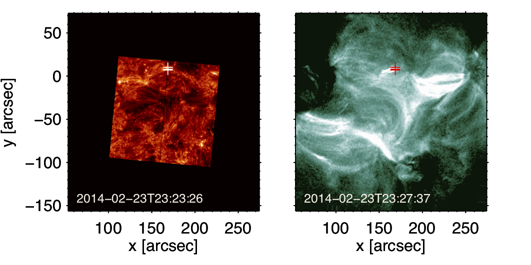
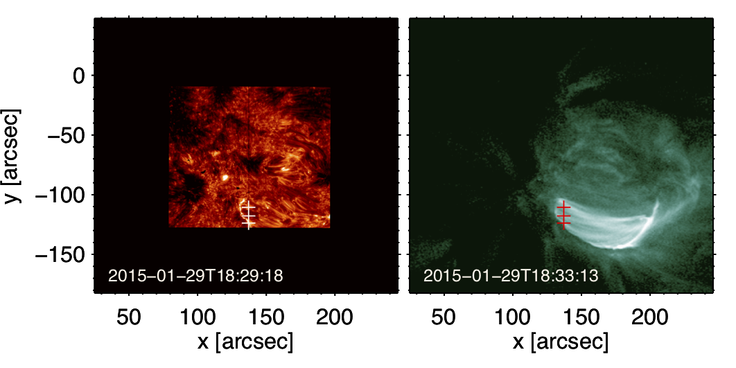
Figure 1: IRIS 1400Å slit-jaw images (left) and AIA 94Å images (right) for two events showing rapid moss brightenings at the loop footpoints (observed in the Si iv $\sim 1400$Å transition region emission) followed (note the different times of the two images) by transient brightenings of the overlying hot ($\gtrsim 5-8MK$) loops (observed in the hot 131Å and 94Å–shown here– AIA coronal images; see also Reale et al. 2019a). The images are coaligned (see text for details) and the crosses show, in both images (in white on the IRIS images, and in red on the AIA 94Å images, for better contrast), the location of the observed moss brightenings analyzed in details in this paper (see also Fig.2 for the event of 2014-02-23–here in the top row–, and Fig.3 for the event of 2015-01-29–here in the bottom row).

We use IRIS calibrated level 2 data, which have been processed for dark current, flat field, and geometrical corrections (De Pontieu et al., 2014), and AIA level 1.5 data, which have been processed for the removal of bad-pixels, despiked, flat-fielded, and image registered (coalignment among the channels, with adjustment of the roll angle and plate scales; Lemen et al. 2012). AIA datacubes in the IRIS field-of-view, already coaligned with IRIS, and in IRIS format, are now available from the IRIS data search pages (and their description and usage is discussed in detail in an IRIS technical note ). The absolute wavelength calibration is already automatically applied to IRIS level 2 spectral data, using neutral lines (such as e.g., the O i 1355.6Å line), which are expected to have, on average, intrinsic velocity of less than 1 km/s (when averaged along the slit; e.g., De Pontieu et al. 2014). However, we also check this calibration by fitting additonal available neutral/photospheric lines (e.g., Fe ii 1392.8Å and S i 1401.5Å in the FUV, and N i 2799.5Å in the NUV). We also apply a deconvolution method to the IRIS spectra, to take into account the effect of the instrument Point Spread Function (PSF), as modeled by Courrier et al. (2018). Courrier et al. (2018) used IRIS observations of a Mercury transit in 2016 to evaluate and model the on orbit IRIS PSF, and provided deconvolution routines for application to IRIS observations (iris_sg_deconvolve.pro). Courrier et al. (2018) noted that spectra of bright and compact brightenings, like the footpoint brightenings we focus on, might be particularly sensitive to PSF effects. We follow the suggestions of Courrier et al. (2018) to limit the number of iterations of the deconvolution algorithm to optimize the deconvolution and avoid fitting noise; in our cases we find that typically $\lesssim 10$ iterations are sufficient in both FUV and NUV.

We also analyze AIA coronal imaging data in six narrow extreme ultraviolet (EUV) channels (94Å, 131Å, 171Å, 193Å, 211Å, 335Å), which sample the transition region and corona across a broad temperature range (Boerner et al., 2012, 2014), and are characterized by $\sim 0.6$ ^′′pixels, and 12 s cadence. We also use the AIA 1600Å images, which have a lower temporal cadence (24 s), for co-alignment between the AIA and IRIS datasets, by applying a standard cross-correlation routine (tr_get_disp.pro, which is part of the IDL SolarSoftware package; Freeland & Handy 1998) to the IRIS 1400Å and the AIA 1600Å images, which typically show many morphological similarities. The co-alignment procedure allows us to remove residual small shifts and the relative roll angle between the two instruments. For the analysis of the temporal evolution of the coronal emission we also correct the AIA time series for solar rotation.

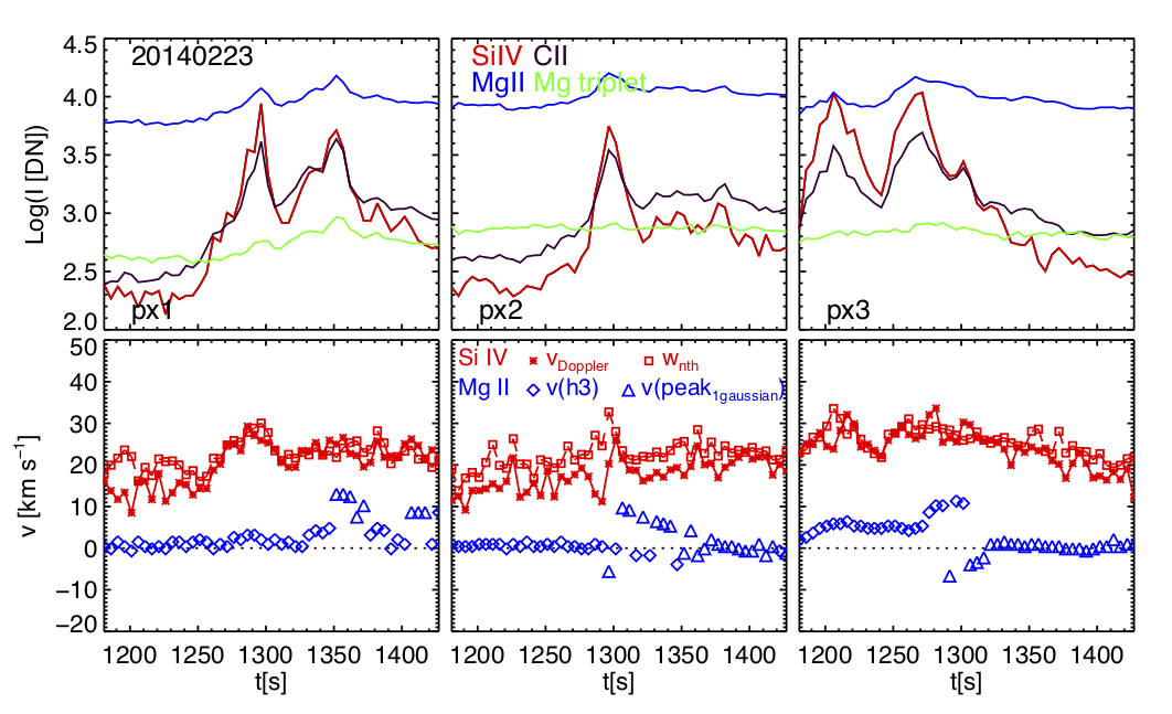
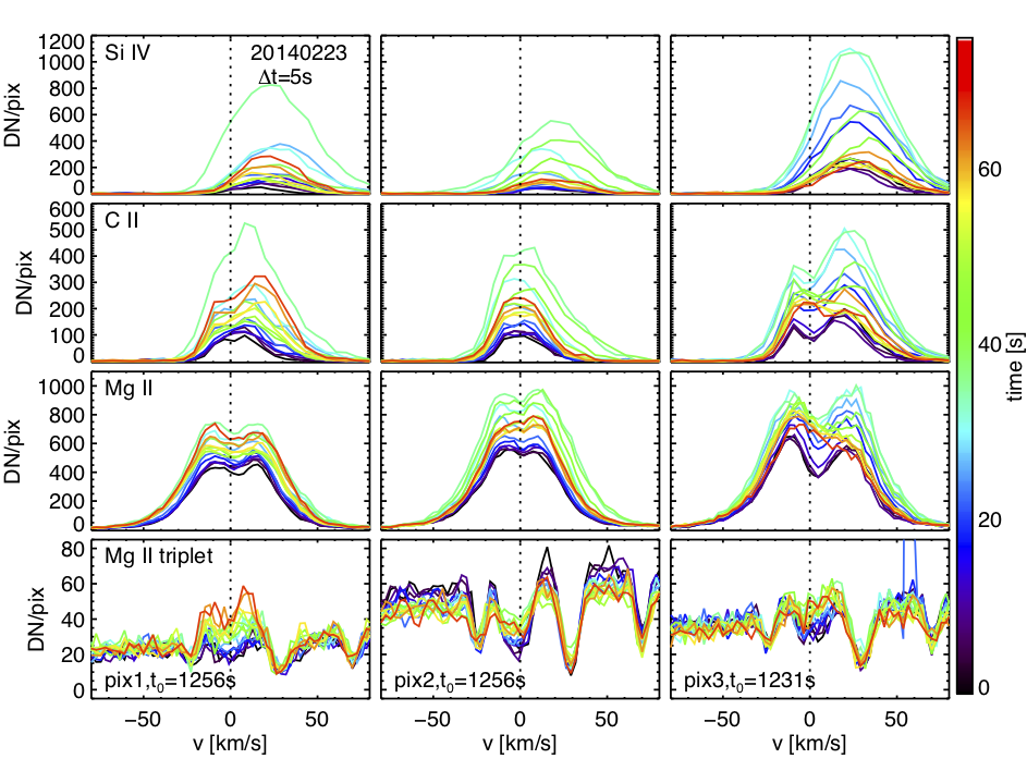
Figure 2: Temporal evolution of IRIS spectral observables, for 3 different pixels (each corresponding to a column) during the moss brightening event observed on 2014-02-23 (as marked in the top row of Fig. 1; event 1 of Table 1). The footpoints locations are ordered (pix1, pix2, pix3) with ascending value of solar y. Top two rows: IRIS spectral line intensities (integrated over spectral profile; top), and Si iv and Mg ii spectral moments (second row) – Doppler velocity and non-thermal line width ($w_{\rm nth}$) from single Gaussian fits to the Si iv 1402.77Å spectra, and Doppler velocity of $h3$ or peak of single Gaussian for Mg ii (see text for details). Negative values (blueshifts) of velocity correspond to upflows, and positive Doppler shifts (redshifts) to downflows. Bottom four rows: spectral line profiles, as a function of velocity, for each time step, color coded as indicated in the color bar on the right.

In the main text of this paper we describe in detail two examples (no. 1 and 6 of Table 1) and show relevant plots, while the corresponding figures for the other datasets are in Appendix A to improve the readability of the paper.

Fig. 1 shows TR and coronal images for these two datasets: the IRIS slit-jaw images (SJI) in the 1400Å passband are typically showing TR ($T\sim 10^{5}$ K) emission (including the strong Si iv 1402.77Å line, which is one of the main targets of our analysis), while the AIA 94Å passband has both a cool ($T\sim 10^{6}$ K) and a hot ($T\sim 8$ MK) peak in the temperature response (e.g., Boerner et al., 2014; Cheung et al., 2015) but its emission in the bright transient loops in the active region core is generally dominated by hot plasma (e.g., Testa & Reale, 2012). The TR footpoint brightenings precede the peak of the hot coronal emission, therefore we show coronal images for later times (seconds to few minutes) so that the hot coronal loops are brighter and better visible. In this Figure (as well as in the other Figures 7-14 in Appendix A) we mark (with crosses) the locations, at the loop footpoints, for which we discuss in detail the temporally resolved IRIS spectra of the rapid brightenings. The moss brightenings are often observed at different times (i.e., they are not all co-temporal), and since we show a single image (both for the IRIS 1400Å SJI, and the AIA 94Å), this accounts for some discrepancy between the location of the TR brightenings and the apparent footpoints of the hot loops, which are rapidly evolving (e.g., bottom row of Fig. 1).

For each event we derive a peak emission intensity in the AIA 94Å coronal band, and an estimate of the duration of the coronal event (column 8 and 9 of Table 1 respectively). We also use the AIA 94Å images to estimate the projected loop length (in the plane-of-the-sky; column 7 of Table 1). The derived projected loop lengths should only be considered as approximate values given that several of these events involve a large number of loops, with a broad range of geometries, and it is sometimes difficult to clearly trace the loop rooted in a particular moss location. However, even with these uncertainties, the values we find show that rapid moss variability occurs at the footpoints of hot coronal loops with a wide variety of properties. The two examples in Fig. 1 showcase this large range of coronal properties, with event 1 being characterized by short loops, with coronal emission which is relatively faint and short-lived (few minutes), and event 6 involving instead a large number of longer loops with high and long lasting coronal emission. In fact, hot loops of event 6 appear to be bright, though highly variable, for a long time in the AIA 94Å passband, and the heating episodes observed by IRIS for this event appear to be part of an ensemble of repeated heating releases.

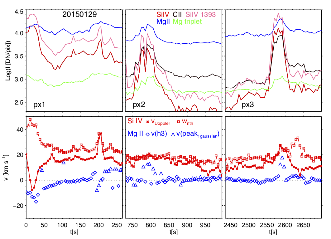
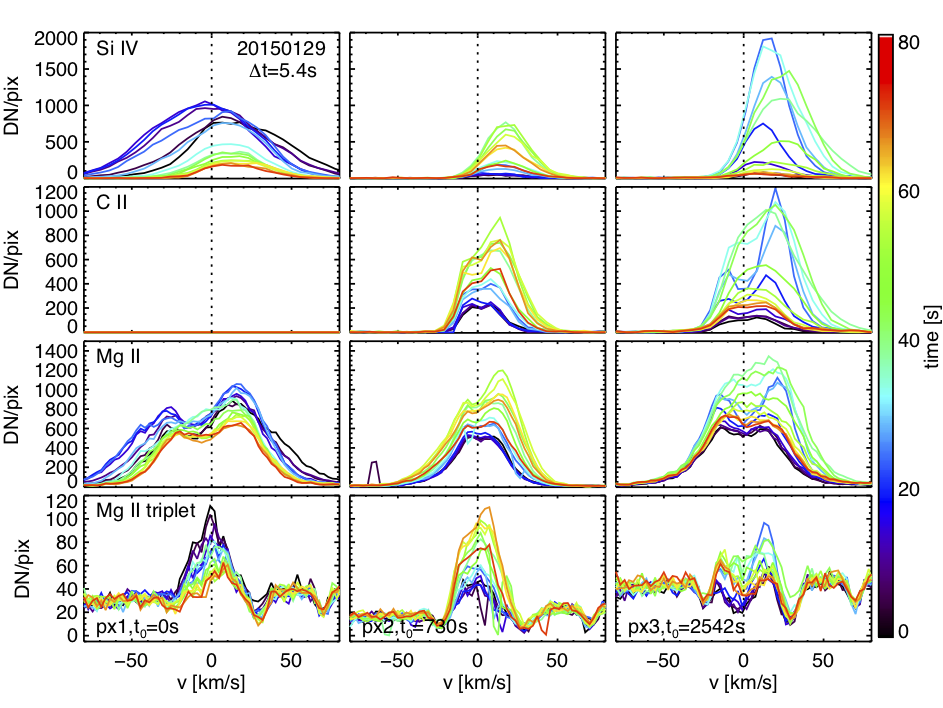
Figure 3: Temporal evolution of IRIS spectral observables, for 3 different pixels (each corresponding to a column) during the moss brightening event observed on 2015-01-29 (as marked in the bottom row of Fig. 1, and ordered by increasing value of solar y; ; event 6 of Table 1), in the same format as for Fig.2. We note that for px1 the C ii spectrum is not available as that footpoint was at the edge of the detector and the shorter wavelength end of the FUV spectrum was outside the detector.

In Figures 2 and 3 we show the IRIS spectral observations for the footpoint brightenings marked in Fig. 1, and the results of our spectral analysis. In our investigation we particularly focus on the following lines: the Si iv 1402.7Å (and Si iv 1393.8Å, whenever included in the IRIS OBSID line list) transition region line ($\log T[K]\sim 4.9$), and the chromospheric C ii 1335Å ($\log T[K]\sim 4.5$; we note that C ii has both a chromospheric and TR nature, see e.g., Rathore & Carlsson 2015) and Mg ii h&k (around 2803Å and 2796Å respectively; $\log T[K]\sim 4.3$) and Mg ii 2798.8Å triplet ($\log T[K]\sim 4.3$) lines. We show the lightcurves obtained by integrating the line intensity over the spectral profile. For the plots of both the lightcurves and the spectral profiles we did not normalize by exposure time in order to maintain the information on signal-to-noise ratios typical of different observations. To obtain uniform estimates of the spectral properties of the Si iv and Mg ii lines for the whole sample, we carried out spectral fits as follows. For the Si iv lines we perform a single Gaussian fit, and derive the Doppler shift ($v_{\rm Doppler}$) of the line centroid and the line width. From the measured line width we derive the non-thermal line broadening ($w_{\rm nth}$), i.e., the broadening in excess of the thermal ($w_{\rm th}=\sqrt{2K_{\rm B}T/m_{\rm ion}}$), and instrumental (for IRIS is of the order of 3.5 km s^-1; De Pontieu et al. 2014) broadening. Note that here we refer to line broadening as $w_{\rm 1/e}$ (in km s^-1), which is the $1/e$ spectral line width, and which corresponds to $\sqrt{2}\times$ the Gaussian $\sigma$, and FWHM/$(2\sqrt{ln(2)})$. The Mg ii lines have more complex spectral profiles, and different IRIS routines are available in the IRIS branch of SolarSoft for the Mg ii spectral fitting using different approaches. Here we use the routine iris_master_fit, described in Schmit et al. (2015), which has been optimized for the fitting of observed IRIS Mg ii spectral profiles. The fit typically uses a double Gaussian plus a linear function, however, in cases where the observed profiles is single peaked it provides the parameters of a single Gaussian fit. Therefore, in our plots of Fig. 2 and  3 (and Fig. 7-14 in Appendix A) for Mg ii we show the Doppler shift of the Mg ii $h3$ feature (${\rm v(h3)}$) or the Doppler shift of the centroid of the single peak (${\rm v(peak_{\rm 1gaussian})}$) , depending on whether the profile is double or single peaked respectively. While these spectral fits generally provide a good estimate of the spectral moments of the Si iv and Mg ii profiles, some particularly unusual and complex profiles are not well fitted by these fitting functions.

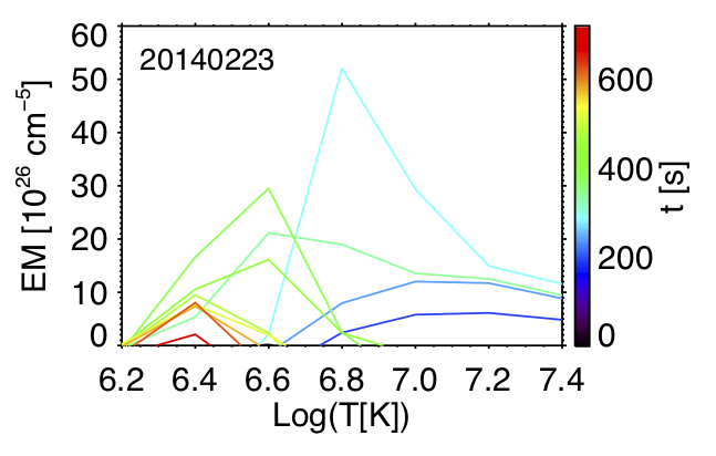
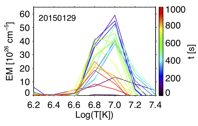
Figure 4: Emission measure (EM) distributions vs temperature (after subtraction of the EM prior to the heating event) at progressive times, color coded as indicated by the color bars on the right, for the two events of Fig. 1. The reference times are 2014-02-23T23:21:43, and 2015-01-29T18:28:07 respectively.

The observed chromospheric and TR footpoint brightenings are typically characterized by an increase in Si iv intensity of an order of magnitude, though this increase factor ranges from less than 2 in the smallest events (e.g., event 5 in Fig. 10, for which however the brightest footpoints are missed by the IRIS slit), to about 2 orders of magnitude (or more, for e.g., some examples shown in Testa et al. 2014) in the brightest events (e.g., event 10 in Fig. 14). Also, the duration of the brightenings is generally short ($\lesssim 60$s), and very similar for all of the events. Generally the Si iv brightenings are accompanied by significant brightenings in the Mg ii and C ii chromospheric lines as well, however in our sample there are also two events for which that is not the case and either Mg ii (event 7; Fig. 11) or C ii (event 5; Fig. 10) present only a very small increase in intensity, if any. The Mg ii triplet (around 2799Å) which, as we we will discuss in more detail in the following sections, provides interesting diagnostics of low chromospheric heating (Pereira et al., 2015), is observed in emission for some locations in a subset of the events in our sample (4 out of 10 events). As in the event we studied in detail in (Testa et al., 2014), the brightenings for which we have IRIS spectra, show a broad range of Si iv Doppler shifts, relative to the line shift before the event, including redshifts (i.e., downflows), blueshifts (i.e., upflows), or no significant shifts. Also, the Si iv lines during most of the brightenings show small or no significant increase in broadening, however with a few notable exceptions including for event 6, for which a footpoint brightening shows very broad but still fairly (single) Gaussian profiles (pix1, Fig. 3), and event 8 (Fig. 12) and 9 (e.g., pix3, Fig. 13), for which the Si iv profiles during the event become quite complex with several components.

Table 2: RADYN simulations discussed in detail.

Model	Name	ET	F	EC	$\delta$	duration
		[1024 erg]	[erg s-1 cm-2]	[keV]		[s]
C1	TC	6	-	-	-	10
E1	5keV	6	1.2 $\cdot$ 109	5	7	10
E2	10keV	6	1.2 $\cdot$ 109	10	7	10
E3	15keV	6	1.2 $\cdot$ 109	15	7	10
H1	10keV+TC	6	0.6 $\cdot$ 109	10	7	10
E4	10keV, 30s	6	0.4 $\cdot$ 109	10	7	30
H2	10keV+TC, 30s	18	0.6 $\cdot$ 109	10	7	30
E5	15keV, 30s	18	1.2 $\cdot$ 109	15	7	30
E6	10keV, 20s_p	6	0.6 $\cdot$ 109	10	7	20 + 60

Table 3: IRIS spectral properties of RADYN simulations of Table 2.

Model	Si iv		C ii	Mg ii	Mg ii triplet
	Doppler	line shape
	shift
C1	red		weak; redshift; stronger rp	weak; peculiar shape; stronger bp
E1	red	multi-component	broad; redshift; stronger rp	broad; redshift; blue tail
E2	blue		symmetric	stronger bp	Y
E3	blue	weak Si iv	stronger rp	symmetric	Y
H1	blue	multi-component	slightly stronger rp	slightly stronger bp
E4	blue	blue tail	stronger rp	symmetric
H2	blue	multi-component	$\sim$ symmetric; red tail	broad; redshift; blue tail	Y
E5	blue		small blueshift; red tail	complex profiles; strong broad bp	Y
E6	blue	blue tail	stronger rp	symmetric; small redshift
	blue	with red tail	small redshift; broad, red tail	symmetric

In Reale et al. (2019a) we have analyzed in detail the coronal emission in the overlying loops, and its evolution, and speculated on the possible role of large-angle magnetic reconnection for these events. Therefore here we only briefly derive and discuss the coronal properties of these coronal heating events showing significant footpoint brightenings. We use the AIA timeseries (in the 94Å, 131Å, 171Å, 193Å, 211Å, 335Å passbands) to derive the emission measure as a function of temperature, using the inversion method of Cheung et al. (2015). The observed emission ($I_{i}$, in units of ${\rm DN~{}s^{-1}~{}pix^{-1}}$) in the AIA narrow-band EUV channels depends on the thermal properties of the optically thin coronal plasma in the pixel, as $I_{i}=\int_{T}R_{i}(T)~{}DEM(T)~{}\,dT$, where $R_{i}(T)$ is the response function in a given passband (in units of ${\rm DN~{}cm^{5}~{}s^{-1}~{}pix^{-1}}$), and the differential emission measure (in units of ${\rm cm}^{-5}~{}{\rm K}^{-1}$) is defined by $DEM(T)~{}\,dT=\int_{z}n_{e}^{2}(T)~{}\,dz$, where $n_{e}^{2}(T)$ is the electron density of the plasma at temperature T. The distribution of emission measure (EM, in units of ${\rm cm}^{-5}$) as a function of temperature which we will show in several plots throughout this paper is obtained by integrating the $DEM(T)$ over 0.2 $\log T$ temperature ranges. In Figure 4 we show the temporal evolution of the emission measure distribution for the coronal loops of the events shown in Fig. 1-3. These plots show coronal temperatures of $\log T\sim 6.8-7.0$ associated with these heating events, as also discussed in more detail by Reale et al. (2019a).

3 RADYN numerical simulations

In our previous work (Testa et al., 2014; Polito et al., 2018) we demonstrated the importance of numerical simulations for the interpretation of the observations. In Polito et al. (2018) we used RADYN 1D HD loops simulations to investigate the plasma response to impulsive heating, for varying heating properties and initial conditions. In particular we focused on the predicted optically thin emission (TR emission in the IRIS Si iv line and coronal emission in the AIA 94Å passband), and we also discussed some properties of the predicted IRIS Mg ii emission.

In the previous section we have presented an analysis of the IRIS chromospheric and TR spectral observations, which can provide much tighter constraints on the properties of the heating. Therefore we expanded on our previous investigation of RADYN nanoflare heated loops, by calculating the synthetic chromospheric emission in C ii and Mg ii triplet for the simulations previously discussed in Polito et al. (2018). The very broad variety of properties of the spectral observations analyzed in the previous section (section 2) motivated us to also explore a few additional simulations to explore different properties of the heating including: (a) combining heating by thermal conduction and non-thermal particles; (b) longer heating duration of 20-30 s; (c) repeated heating in the same loop (in particular, two 20s heating episodes separated by 60 s intervals when the heating is switched off).

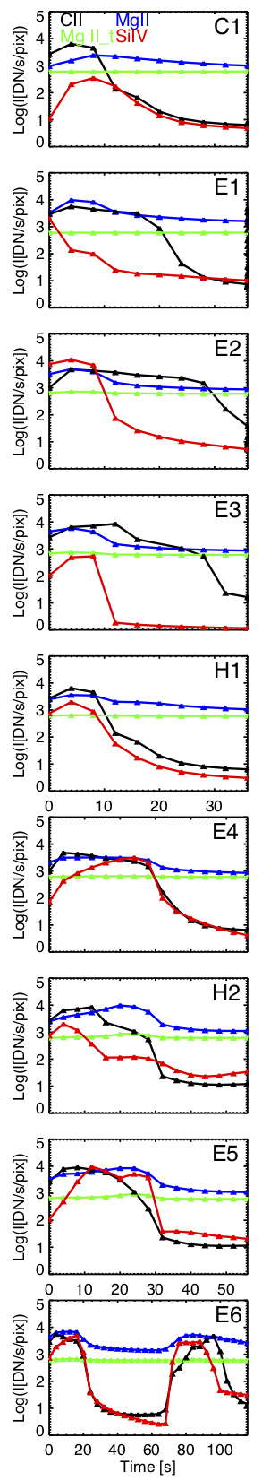
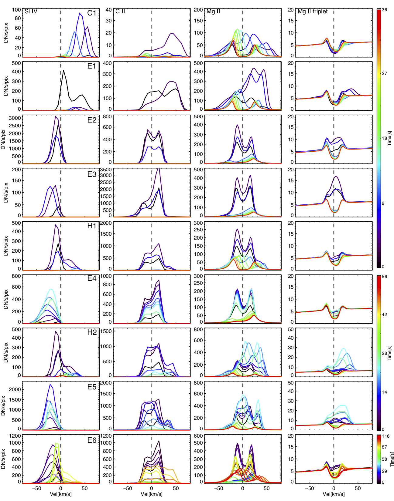
Figure 5: Left column: Synthetic lightcurves in IRIS spectral lines as derived from the RADYN simulations of Table 2. These predictions are calculated by assuming an integration time (and cadence) of 4 s (i.e., the data point at t=0 corresponds to the average intensity in the first 4 s since the onset of heating), and can be directly compared with the observed lightcurves (top panels of Figures 2 and 3, and Figures 7-14 of Appendix A). Right four columns: Temporal evolution of corresponding synthetic IRIS spectra, in the same format as the observed spectra (bottom plots of Figures 2 and 3, and Figures 7-14 of Appendix A for the other studied events). These synthetic spectra are obtained by assuming an integration time (as well as a cadence) of 4 s, which is similar to most of the observations studied here (see Table 1). We note that, due to the different duration of the heating in the different models the timescales are different for the first 5 rows (36 s; models C1, E1, E2, E3), row 6-8 (56 s; models E4, H2, E5), and the last row (116 s, model E6).

The details of the RADYN numerical code (Carlsson & Stein, 1997; Allred et al., 2005, 2015) and the general description of how these simulations of nanoflare heated loops are run are discussed in detail in Polito et al. (2018), so here we only provide a brief description. The RADYN code solves the 1D equation of charge conservation and the level population rate equations for the magnetically confined plasma; the loop’s atmosphere encompasses the photosphere, chromosphere, TR, and corona. RADYN is ideal for our investigation because of (a) it includes non-local thermodynamic equilibrium (non-LTE) radiative transfer, which is necessary to model the chromospheric emission, and (b) it allows to model heating by non-thermal electron (NTE) beams (Allred et al., 2015). As discussed by Polito et al. (2018) we added chromospheric heating to obtain a more realistic plage-like atmosphere as in Carlsson et al. (2015). The IRIS Si iv optically thin emission is synthesized from the model by using atomic data from CHIANTI (Dere et al., 1997; Landi et al., 2012; Del Zanna et al., 2015a) and assuming ionization equilibrium, as in Polito et al. (2018). The IRIS optically thick C ii, Mg ii, and Mg ii triplet emission is synthesized by using RH1.5, which is a massively-parallel code for polarised multi-level radiative transfer with partial frequency distribution (Pereira & Uitenbroek, 2015). We have performed dozens of RADYN simulations of nanoflare-heated loops investigating a broad parameter space, including different:

• nanoflare energies: 10²⁴ to 10²⁶ ergs

• loop top temperatures : T_LT = 1, 3, and 5 MK

• half-loop lengths L/2 = 15, 50 and 100 Mm

• heating models: (a) thermal conduction (TC), (b) electron beam (EB) heating with different energy cut-offs E_C = 5, 10 and 15 keV, and (c) TC + EB hybrid models

Some of these simulations have already been presented in detail in Polito et al. (2018). In the following we discuss in detail nine of these (dozens of) simulations summarized above, for which the synthetic spectra have characteristics similar to the observed spectra in terms of e.g., duration of the brightenings and line intensities (see discussions in Sec. 4 and 5). In particular, as summarized in Table 2, we selected four of the simulations presented in Polito et al. (2018) – with an initially empty cool loop ($T\sim 1$ MK), of semi-length of 15 Mm, heated for 10 s by TC or NTE with 5/10/15 keV energy cutoff –, and five new simulations, all run on the same cool initial condition: (1) 10 s heating with TC and NTE with 10 keV cutoff (and total energy of $6\times 10^{24}$ ergs, as in the previous runs), (2) intermittent heating (two 20 s heating episodes with 60 s pause in between) by NTE with 10 keV cutoff, (3) 30 s heating by NTE with 10 keV cutoff, (4) 30 s heating with TC and NTE with 10 keV cutoff, and total energy of $1.8\times 10^{25}$ ergs, (5) 30 s heating by NTE with 15 keV cutoff, and total energy of $1.8\times 10^{25}$ ergs.

Figure 5 shows the predicted IRIS lightcurves (left column) for the nine selected RADYN simulations, synthesized by assuming an integration time (and cadence) of 4 s. A qualitative comparison of these synthetic lightcurves with the observed ones (shown in Fig. 2, 3, 7-14) shows in general a very good agreement between simulations and observations in terms of intensities and durations of the brightenings. As observed, the relative increase of emission in Mg ii is, typically, significantly smaller than in Si iv or C ii. We will discuss this comparison in more detail in section 4.

Figure 5 shows the temporal evolution of the synthetic IRIS spectra for the selected simulations, in the same format used for the observations in Fig. 2 and 3. The spectra are obtained by assuming an integration time and cadence of 4 s, similar to many of the studied observations, and applying the appropriate thermal and IRIS instrumental broadening, and assuming a spectral bin of 0.025Å for all spectral lines (i.e., corresponding to a binning of $\times 2$ in FUV and original spectral resolution in NUV, which is a quite typical observing mode for these nanoflare observations, due to the typically higher S/N in NUV).

First of all, the synthetic spectra show a very broad variety of spectral line profiles, similarly to the observations. For instance, the Si iv emission in several cases shows a complex transient multiple component profile (e.g., 5 keV, 10 keV+TC).

The Mg ii emission sometimes shows unusual profiles, similar to what is occasionally observed (see e.g., Fig. 10,  13). We note that, despite our efforts in creating a more realistic plage-like atmosphere, some of the observed filled in (single Gaussian) Mg ii profiles are not easily reproduced by the simulations (see also discussion in Polito et al. 2018).

The Mg ii and C ii synthetic profiles with a strong increase of the red peak to blue peak ratio (e.g., C ii profile for the 15 keV case of Fig. 5), are usually due to an upflow which causes a blueshift of the $\tau_{\nu}=1$ layer which causes in turn the increased absorption of the blue peak. Analogously, profiles with a higher blue peak (e.g., Mg ii profile for the 10 keV case of Fig. 5) can be caused by downflows causing an increased absorption of the red peak.

A notable results concerns the Mg ii triplet, which in our simulations are predicted to be strongly in emission only if high energy NTE are present. This is due to the fact that, in our modeled atmospheres, the Mg ii triplet is much more sensitive to heating in the lower chromosphere, close to the temperature minimum, than the C ii and Mg ii chromospheric lines, and it is therefore expected to be in emission only if those lower chromospheric layers are significantly heated (see Pereira et al., 2015, for a detailed discussion of the Mg ii triplet formation mechanism). This is a very important finding as it results in a new diagnostic of the presence of NTE in these events.

In Table 3 we summarize some of the main spectral properties of the IRIS synthetic spectra from our simulations, for easier comparison with the observations (see Sec. 4 and Table 4).

4 Discussion

In Sections 2 and 3 we have discussed respectively the observed and modeled IRIS spectral properties of transition region brightenings arising in response to impulsive coronal heating. The simulations presented in Section 3 (and also in Polito et al. 2018) have not been run to forward fit the specific observations presented here, but they do explore a relatively broad parameter space and can be used for a qualitative comparison with the observations, and their interpretation. In order to investigate the qualitative agreement between the predicted and observed spectral properties we first construct histograms of the spectral properties derived from the IRIS observations. In Figure 6 we show histograms for the Doppler velocity and non-thermal broadening (at peak intensity) of the Si iv line, for the duration of the TR brightening (defined as the time interval when $I>I_{\rm max}/e$ for Si iv), and for the ratios of the peak intensity values of Si iv, C ii, Mg ii (in particular we show the C ii/Si iv, and Mg ii/Si iv ratios), all measured from the observed IRIS spectra. We note that here we take into account all the different footpoint brightenings, as for many events there is more than one footpoint brightening observed by IRIS. We show the C ii/Si iv, and Mg ii/Si iv intensity ratios because the are a useful diagnostics of the relative amount of energy deposited in different atmospheric layers, as predicted from the models (see Fig. 5 and Table 3). These histograms show that the observed brightenings are characterized by:

• Si iv relative Doppler velocity with a broad distribution, quite symmetric around zero, and with absolute values $|{\rm v_{Doppler}|\lesssim 40}$ km s^-1

• generally modest non-thermal broadening increases, with only a few footpoint brightenings (e.g., event 6, Fig. 3) showing large values of $w_{\rm nth}$, up to 40 km s^-1; we note that some of these broader spectra still have Gaussian profiles (e.g., event 6, Fig. 3), while others clearly show multiple components or more complex non-Gaussian profiles (e.g., event 8, Fig. 12, and event 9, Fig. 13)

• short duration ($\lesssim 30$ s)

• similar intensity increases in Si iv and C ii (with C ii/Si iv typically $\sim 0.5$-$1$), whereas the brightening intensity in Mg ii appears less closely tied to the Si iv emission

We note that we made specific choices in the definition of the variables shown in Fig. 6, and that a single value might not adequately capture the complexity of some footpoint brightenings. For instance, for some brightenings (e.g., pix 2 and pix 3 of event 1, second row of Fig. 2) the Si iv line appears to undergo an initial blueshift followed by a redshift (also reproduced e.g., by model H2; see below for further discussion).

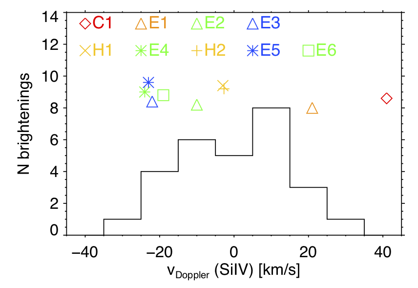
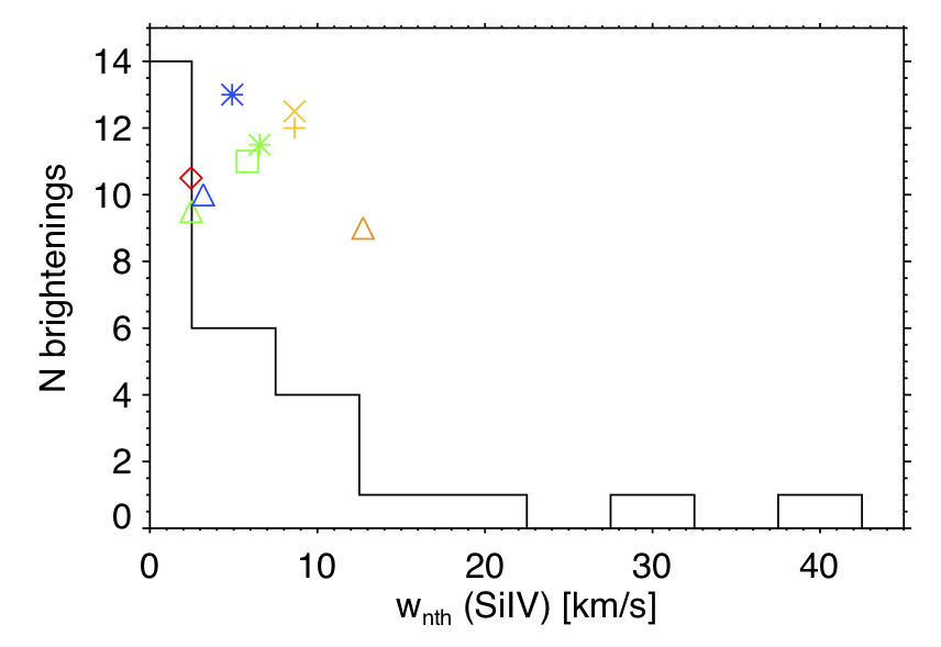
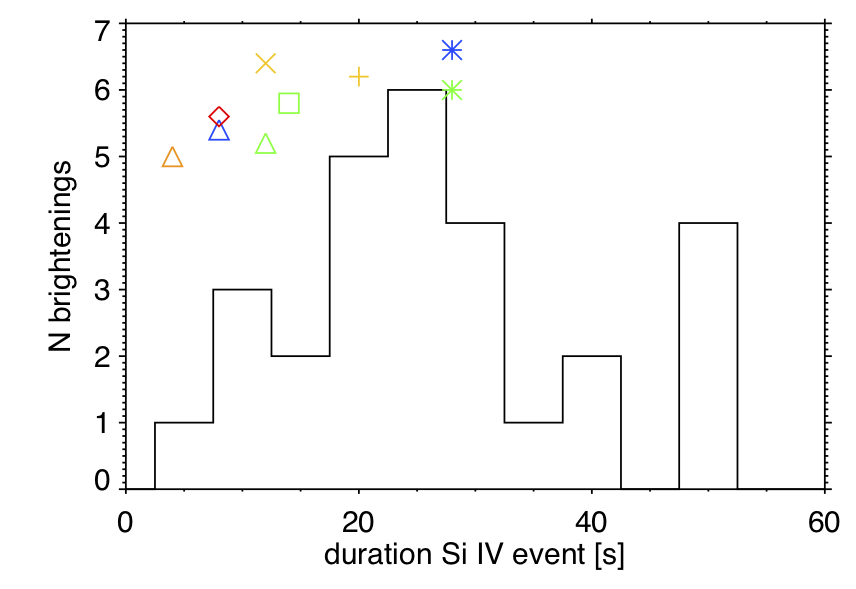
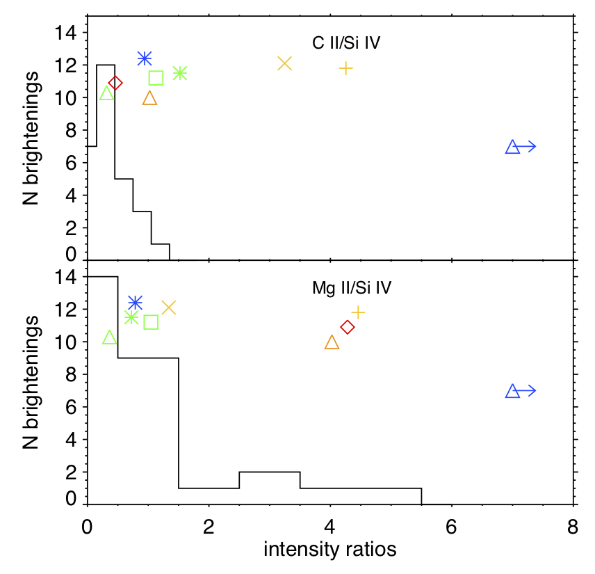
Figure 6: Histograms of observed properties of footpoints brightenings observed by IRIS, and associated with coronal heating events (from top): Si iv Doppler velocity, Si iv non-thermal line broadening, duration of the moss brightening in Si iv (where $I>I_{\rm max}/e$), ratio of intensity maxima for C ii/Si iv and Mg ii/Si iv. The colored symbols show the corresponding predictions of the different RADYN models (see legend in the top panel) described in the text (and Table 2-3, Figure 5. Each symbol corresponds to one RADYN simulation, and we offset the values in the y direction in order to make them distinguishable even when different simulations have similar values of the shown parameters.

We derive the analogous spectral properties from the synthetic spectra of the simulations (sec. 3), and superimpose them on the histograms of measured values in Figure 6. Similarly to the observations we note that a single value might not capture the complexity and evolution of the predicted IRIS spectral properties. This comparison shows that the RADYN simulations of nanoflare heated loops can reproduce most of the observed properties. In particular, the simulations reproduce well the observed range of: (a) duration and Doppler shifts of the Si iv TR emission, (b) relative ratio of chromospheric to TR emission, and (c) variability of emission.

A closer look to this overall comparison of the observed range of parameters with the predictions of our models reveals some of the constraints the observations put on the simulations, and it also provides useful guidance on how to further extend the exploration of the parameter space with future simulations. For instance, the large redshift predicted by our TC simulation (model C1) is beyond the range of observed Doppler shifts, indicating that in these nanoflares, if/when TC (and/or NTE with low $E_{C}$) is dominating the energy transport, the initial density might likely be larger than assumed in these models (see e.g., for comparison the hot/dense models in Polito et al. 2018) and/or the energy released in the single event (and energy flux) might be smaller (see Polito et al. 2018). We also note that only two of the selected models predict Si iv redshifts (C1, and E1), while several observations show redshifted Si iv. However, different combinations of heating – e.g., NTE distributions, different duration of TC and NTE heating, total energy (see e.g., Fig. 15 of Polito et al. 2018 which shows that larger events can have redshifts at larger $E_{C}$)– and initial conditions can reproduce a broader range of Si IV Doppler shifts. Similarly, the hybrid models (H1, H2) predict a larger than observed C ii/Si iv ratio, suggesting that more realistic models might need for instance slightly different partition of energy between NTE and TC (in the models for this paper we assume the energy is equally divided between the two transport mechanisms). Therefore, as a follow-up work we will explore simulations using initial conditions with intermediate density/temperature between the cool/empty (1 MK) and the hot/dense (3 MK) initial atmosphere used in Testa et al. (2014); Polito et al. (2018) and here, and explore different heating properties. Additional effects, such as e.g., non-equilibrium ionization, are also expected to increase the predicted Si iv emission and likely bring the C ii/Si iv and Mg ii/Si iv intensity ratios expected from our simulations in better agreement with the observations.

We also note that our loop models are generally characterized by modest non-thermal broadening, therefore not reproducing the large non-thermal broadening observed for a few footpoint brightenings. This discrepancy might either be due to physical processes missing from our simulations (e.g., turbulence; we note that lack of non-thermal broadening has been found also for 3D MHD simulations, as e.g., discussed by Testa et al. 2016) and/or imply a more complex scenario of multiple loops (possibly with different initial atmosphere) simultaneously heated with different heating properties (see e.g., Polito et al. 2019 for an example of multi-loop 1D RADYN modeling though applied to larger flares), or, depending on the viewing angle, the presence of waves or turbulence that leads to broadening in the direction perpendicular to the field. Another limitation of our models is that the line profiles of the Mg ii and C ii chromospheric emission are not always well reproduced, especially the single peaked profiles (typical of plage) as previously remarked by Polito et al. (2018) (see discussions therein). Finally we also note that the simulations are generally characterized by pre-nanoflare Si iv Doppler shift of $\sim 0$ km/s (and in Fig. 6 the observed Si iv Doppler shifts are the values relative to the pre-nanoflare ”rest” velocity), while the observations (e.g., Figures 2 and 3) often show significant TR Doppler shifts in quiescent conditions (see e.g., Testa et al. 2016 and reference therein for examples of recent studies of TR Doppler shifts).

Notwithstanding their limitations, the simulations can be used as a guide to infer the properties of the heating on a case-by-case basis. However we note that here we will carry out a qualitative comparison, given that the simulations explore a limited range of parameters (e.g., initial conditions, total energy, duration of heating, mix of TC and NTE, properties of NTE,…) and therefore finding a perfect match between observations and simulations is beyond the scope of this paper. Here we discuss in detail the specific observational properties of the IRIS spectra for all the studied events, their similarities with the predictions from our models, and the resulting diagnostics. We summarize these results in Table 4. We categorize the events in three groups characterized by: (a) strong evidence of NTEs, (b) likely presence of NTEs, and (c) lack of significant evidence of NTEs:

• Strongest evidence of NTEs (both Mg ii triplet emission and Si iv blueshifts):

  • Event 1 (Fig. 1, top, and Fig. 2) is a short lived heating event in small loops, but it nevertheless shows significant Mg ii triplet emission at (at least) one of the footpoints, which, as discussed in §3 points to the presence of NTE. The chromospheric emission in px 1 is similar to models E2-E3, though the lack of corresponding Si iv blueshift suggests a mix with heating by TC (e.g., H1). The other two footpoints (px 2 and px 3) show a peculiar initial relative blueshift in Si iv immediately followed by a redshift similar to model H2 (though we observe Si iv profiles generally well approximated by a Gaussian). For these footpoints also the chromospheric emission is well approximated by hybrid models (H1,H2) which also reproduce the initial larger increase of the Mg ii blue peak, the absorbed red peak emission in Mg ii in the later phases of the event (e.g., H1), as well as the small increase of the Mg ii triplet emission and the small red tail in the C ii emission.

  • Event 6 (Fig. 1, bottom, and Fig. 3) is one of the largest events in our sample, with intense, relatively long-lasting ($\sim 1000$ s) and morphologically complex coronal emission. In this event, all the studied footpoints have strong Mg ii triplet emission, indicating significant presence of NTE, and one of the footpoints (px 1) has Si iv emission characterized by strong blueshift and line broadening. The Si iv and Mg ii spectra of px 1 are similar to model E3, though our simulation does not reproduce the unusually broad profiles. The other two footpoints (px 2 and px 3) show no shift (px 2) or modest redshift (px 3) in Si iv (see Fig. 3), and their IRIS spectra are overall similar to model H2.

  • Event 8, although characterized by relatively weak coronal emission (see Table 1) shows quite strong TR and chromospheric brightenings (including some Mg ii triplet emission for px 1), with some complex line profiles (Fig. 12), somewhat similar to model H2 (Fig.5). Also the spectra of the other two analyzed footpoints (px 2 and px 3) present similarities with the hybrid models (H1 and H2), although with a stronger red component in the Si iv emission possibly indicating a stronger contribution of TC compared with NTE for these two footpoints. We also note that this event is the only event in our sample presenting a significant increase in continuum emission in the wavelength range around the Mg ii triplet (see bottom plots of Fig. 12).

  • Event 10 presents several peculiarities in its spectral properties (Fig. 14). The Si iv and C ii emission before the brightenings is extremely weak (though we note also the shorter exposure time in this dataset). The Si iv brightenings are blueshifted, and the chromospheric profiles are highly unusual and show a strong emission increase at shorter wavelengths. These features strongly suggest the presence of highly energetic NTE (inversions with the new IRIS² code of Sainz Dalda et al. (2019) also support this conclusion, as we will discuss in detail in a follow-up paper), and it is most similar to model E5. This is also compatible with the very weak overlying coronal emission, because models with highly energetic NTE predict very small coronal emission (because most of the energy is dissipated in the chromosphere; see Polito et al. 2018 for a more detailed discussion). In fact, although the observed IRIS TR/chromospheric brightenings are associated with heating of overlying small transient loops observed in the AIA 94Å passband (see top right panel of Fig. 14), the subset of brightenings under the IRIS slit however are at the footpoints of very weakly emitting coronal loops.

• Likely presence of NTEs (small Si iv blueshifts):

  • Event 2 (Fig. 7) involves very short loops, and presents lightcurves suggesting repeated heating, and an overall longer event likely with lower energy flux than assumed in our simulations. The Si iv spectrum in Fig. 7 shows a small blueshift suggesting the presence of some NTE. The Mg ii and C ii line profiles show a deep central reversal (not common in our simulations while the nanoflare loop is being heated, in particular for C ii), and the evolution of the Mg ii emission similar to models H1 (or E4, E6), including the slightly stronger red peak of C ii and blue peak of Mg ii.

  • In event 3 (Fig. 8) the observed footpoints brightenings are short-lived and intense. The Si iv initial emission is generally quite low, its spectral profiles are close to Gaussian and, at least in some cases, show small blueshifts during the brightenings. The chromospheric C ii and Mg ii profiles are often single peaked, which is not easily reproduced by our simulations. For px 1 the observed emission is closest to models E2-E4 (possibly with lower energy flux, considering the generally weaker observed emission), though, as remarked earlier, the close to single peak C ii and Mg ii profiles are not well reproduced. For px 2 the chromospheric emission, including the C ii line profiles and modest Mg ii triplet emission, is overall similar to models E2 and E4, including the stronger blue peak of C ii and the small red tail in the Si iv profiles.

  • The footpoints brightenings in event 5 (Fig. 10), which has weak and short-lived coronal emission, are barely caught under the slit. The IRIS spectra are characterized by blueshifted Si iv emission, barely detected C ii emission, unusual Mg ii profiles, and no significant Mg ii triplet emission. The Si iv blueshifts suggest the presence of some NTE, while the Mg ii profiles are reminiscent of models C1 and E1, which together with the small intensity increases suggest compatibility with lower energy nanoflares (e.g., see model with total energy of $10^{24}$ erg in Polito et al. 2018, which produces blueshifted Si iv emission).

• Lack of evidence of NTEs:

  • Event 4 (Fig. 9), observed in the same AR a few hours later than event 3, is characterized by relatively weak but long-lasting coronal emission. The brightenings observed in the TR and chromosphere are small (especially in Mg ii), short-lived, and generally without large Si iv Doppler shifts. The Si iv spectral profiles of px 1 are similar to model H1 and the later stages (i.e., second heating episode) to model E6, including the red tail of Si iv emission, while the single peaked chromospheric profiles are not well matched by our models. For px 2 and px 3 the profiles, including the small blueshift in Si iv and the C ii (with its brighter red peak) and Mg ii emission, are similar to models E4-E6.

  • Event 7 is a very small event, both in terms of coronal (see Table 1) and TR/chromospheric emission (Fig. 11), with no significant increase in Mg ii emission. The IRIS spectra are compatible with a very small energy release where the heating transport is dominated by thermal conduction.

  • Event 9 is one of the larger events in our sample in terms of its associated coronal emission, and despite that, it does not show significant Mg ii triplet emission (Fig. 13). The Si iv footpoint brightenings are characterized by either no significant Doppler shift (px 2) or redshift (px 1 and px 3), and the lightcurves generally suggest repeated heating (especially for px 2 and px 3). For px 1 the IRIS spectra are similar to model C1 and E1. For px 2, the brightenings have spectra similar to prediction of models H1-H2 (which however do not reproduce well the deep central reversal observed in the C ii spectra of the first brightening, second column of Fig. 13). The IRIS spectra of the brightening observed in px 3 are more similar to model E1-C1, as in px 1. We note though that the lack of clear evidence of NTEs does not necessarily imply that there are no NTEs. For example, as shown by Polito et al. (2018) (their Fig. 15), for larger energies ($\sim 10^{25}$ erg) also heating by higher energy NTE ($\sim 10$ keV) can produce Si iv redshifts.

Table 4: Observational properties of IRIS spectra and comparison with models, for the events of Table 1.

No.	Si iv	Mg ii	comments	closest model(s)
	Doppler shift	triplet
1	red; blue then red	Y	small C ii and Mg ii central reversal	H1, E2, E3, H2
2	blue		deep central reversal	H1
3	blue; negligible; red		small central reversal/single peaked C ii and Mg ii	E2, E6
4	negligible; blue; red		small central reversal/single peaked C ii and Mg ii	H1, E4, E6
5	blue		unusual Mg ii profiles, weak C ii emission	E1, C1
6	blue; negligible; red	Y	broad Si iv lines	E3, H2
7	negligible		no Mg ii increase	C1
8	red; blue	Y	continuum enhancement;	H2, H1
			single peaked C ii and Mg ii ; multi-component
9	red; neglibile		unusual (broad, multi-component) profiles	C1, E1; H1, H2
10	blue	Y	blue components strongly enhanced; weak coronal emission	E5

The evidence of accelerated particles in several of these events is a significant indication of magnetic reconnection (e.g., Cargill et al., 2015) as driver of many of these impulsive events. In particular, event 4, 5 and 8, which are analyzed in more detail in Reale et al. (2019a) all present evidence of non-thermal particles. As we discussed in more details in Reale et al. (2019a), the appearance of the coronal emission and its evolution for several of the events in our sample suggests large-angle reconnection, different from the small angle reconnection driven by loop footpoint shuffling as expected in the classic nanoflare scenario of Parker (1983, 1988), and possibly related to a different driver such as flux emergence (e.g., Asgari-Targhi et al., 2019).

5 Conclusions

In this paper we have analyzed a sample of IRIS observations of moss rapid brightenings associated with coronal loop heating, focusing on the spectral properties of the chromospheric and TR response to the coronal heating. The events studied here were manually selected to have an evident associated heating of the overlying coronal loops, as observed in the AIA 94Å imaging data, and so that at least some of the footpoint brightenings are observed under the IRIS spectral slit. Typically we find that the coronal temperatures reached by these nanoflare heated loops are up to $\sim 10$MK (see also Reale et al. 2019a, b). The sample we obtained otherwise shows a very broad variety of coronal properties, with loop lengths, and coronal emission and duration spanning more than an order of magnitude (see Table 1). Despite this broad range of coronal properties the footpoint brightenings observed with IRIS have several similarities, including:

• duration of the brightenings of less than a minute (with median and average of $\sim 25$ s; ; see Fig. 6), and similar in the TR and chromospheric IRIS lines, with the exception of the Mg ii triplet, which is often absent or shorter lived;

• a large variety of spectral properties (e.g., intensity, Doppler shifts, broadening, line ratios) even for different footpoints in the same coronal event (see e.g., Fig. 2 and 3);

• typically small increases of Si iv non-thermal line broadening during the events (see Fig. 6; though there are exceptions, such as e.g., the brightening in the left column of Fig. 3);

• Si iv spectral profiles are typically Gaussian, though a few profiles are briefly characterized by multiple components (e.g., see Fig. 12 for event 8 of Table 1).

We also note that the moss brightenings are often observed at both footpoints (as observed in the IRIS 1400Å SJI or AIA 1600Å; see also Reale et al. 2019a and Testa et al. 2014), though the conjugated footpoint is not observed under the IRIS slit. The simultaneous brightening of both loop footpoints further supports the coronal nanoflare scenario, where magnetic reconnection occurs in the corona and heating is subsequently propagated from the corona to both footpoints simultaneously (at least within the IRIS SJI/AIA cadence), and it seems to be at odds with a scenario in which chromospheric reconnection is the main mechanism responsible for the footpoint brightenings (e.g., Judge et al., 2017).

The RADYN simulations of nanoflare heated loops we have run with different heating properties (e.g., heating transport – by TC, NTE, or combination–, duration and total energy of the heating, energy distribution of NTE) reproduce quite well the observed range of intensity, duration, and Doppler shifts of Si iv brightenings, as well as chromospheric to TR intensity ratios. These simulations provide a useful guide for the interpretation of the observations (see details in §4). We note that even though we mostly find good qualitative agreement between observations and simulations, it is not always possible with the current limited set of simulation parameters to find detailed quantitative agreement for all observed properties. Therefore one of the main conclusions from our analysis is that the combination of all the available spectral information (TR/chromospheric emission), together with the coronal observations, really tightly constrains the heating properties in these impulsive heating events. In Sec. 4 we discussed how the model parameters can be tweaked to improve the agreement between the models and the observations.

Another interesting finding of this work is the powerful diagnostic provided by the Mg ii triplet emission: our simulations suggests that this emission is caused by heating low in the atmosphere, which, in the scenarios we explored, requires the presence of non-thermal particles (see §3; however we note that, as we discuss below, we are currently investigating whether the Mg ii triplet emission might also be caused by Alfv$\acute{\rm e}$n wave heating). Our IRIS observations, for which the Mg ii triplet is observed in emission in at least 4 out of 10 events, suggest that acceleration of particles takes place, and it is not uncommon, also in smaller – nanoflare-size – events, and it is not a prerogative of large flares. Furthermore, we find that evidence of NTE is found also for some of the smaller events (e.g., event 1, Fig. 2), and, at the same time, some of the brightenings in the larger events of our sample appear compatible with models without NTE. However we find that only overall larger events (in terms of both coronal and TR/chromospheric emission; e.g., events 6, 8 and 9) are characterized by larger ($\gtrsim 1$) C ii/Si iv ratios, likely pointing to higher overall energies, larger duration of the events, more energetic NTE (see Fig. 6, and related text; note also that event 6 and 8 both have Mg ii triplet emission, indicating the presence of high energy particles).

Although not all observed spectral properties in a single footpoint brightening are well reproduced by the models we have run, better fits can be found through a more thorough exploration of the parameter space, which will be the focus of follow-up work. The predicted spectral properties in fact critically depend on initial conditions, as well as energy flux and duration of the nanoflare, both of which determine where the energy is deposited.

The events studied here are heating events in the active region core involving several loops, each heated by a nanoflare size energy release, as evidenced by the good qualitative agreement between the simulations and observations (as well as rough estimates based on imaging data, as in e.g., Testa et al. 2013). These type of events have been the focus of earlier studies focused on imaging AIA 94Å observations (e.g., Testa & Reale, 2012; Ugarte-Urra & Warren, 2014; Ugarte-Urra et al., 2017, 2019). However, the additional spectral diagnostics of our studies (Testa et al. 2014 and this paper) clearly improves the diagnostic potential to unveil the properties of coronal heating for the hot AR cores. These studies require high spatial and temporal resolution, as provided by IRIS observations, to reveal the highly transient and localized variability at the loop footpoints and therefore, in turn, the impulsive nature of the heating. We note that, although larger than single nanoflares, the event we analyzed here are nevertheless typically smaller than other small events such as microflares (e.g., Warren et al. 2016), which are also visible with hard X-ray spectrometers such as RHESSI (Hannah et al., 2008). Although new hard X-ray instruments have increased sensitivity (e.g., NuSTAR, Harrison et al. 2013), their ability to constrain non-thermal emission in very small events such as the ones we focus on here is often limited by the presence of a dominant thermal emission (e.g., Glesener et al., 2017), as well as by observational limitations due to the use of an astrophysics observatory for solar observations (e.g., Hannah et al., 2019). We note however that these hard X-ray observations are generally compatible with the NTE distributions suggested by our analysis. For instance, Wright et al. (2017) find for a very small event (characterized by temperature of only $\sim 5$ MK, significantly smaller than in our events) that the NuSTAR spectrum is compatible with $E_{C}\lesssim 7$ keV and $\delta\gtrsim 7$ (here we assume $\delta=7$ for all our simulations).

The sample analyzed here is of limited size due to the manual search (which has been restricted to sit-and-stare or few step rasters, and short exposure times) and the general difficulty of finding these footpoint brightenings under the slit. However, we are now working on follow-up work which will allow us to overcome this shortcoming, by using automated detection. Graham et al. (2019) recently presented an algorithm, improved from the one we used on Hi-C data (Testa et al., 2013), which allows us to automatically detect rapid moss variability in AIA timeseries. We are currently working on applying this algorithm to AIA datacubes co-aligned with IRIS data (already available on the IRIS data search webpage ), to automatically find these brightenings in IRIS spectral data. This approach will allow us to greatly expand the sample analyzed here and derive more statistically significant properties for this type of events. The automated approach will also allow to (at least partially) overcome the bias in the selection toward larger events likely affecting the sample in this paper (we manually selected events with relatively high hot coronal emission).

Another issue that we are addressing in follow-up work is the qualitative nature of the comparison we carried out here between observations and RADYN simulations to deduce the heating properties compatible with the observables. We plan to devise a more robust method for this comparison, and the interpretation of the IRIS observations. In particular, we plan to run RADYN simulations on much finer grid of parameters (as partly discussed in the previous section 4) exploring a larger parameter space (e.g., initial conditions, duration of the heating, combination of TC and NTE, total nanoflare energy, parameters of NTE), and to find the closest matches to the observed spectra by using an automatic algorithm such as e.g., k-means clustering (e.g., Panos et al., 2018) or using neural networks (e.g., Osborne et al., 2019). This will also be complemented by using the IRIS² inversion code of Sainz Dalda et al. (2019) for all of our events to obtain further constraints on the initial atmosphere and on the response of the lower atmosphere to small coronal heating events.

Finally, another aspect we are exploring is whether some of these events could be dominated by heating from dissipation of Alfv$\acute{\rm e}$n waves rather than non-thermal electrons. Such heating has been implemented in RADYN and used for flare simulations (Kerr et al., 2016) and we are now studying Alfv$\acute{\rm e}$n wave heating in nanoflare heated loops (Kerr et al., in preparation). Alfv$\acute{\rm e}$n waves are likely to be present, although more difficult than non-thermal particles to constrain observationally, and we want to investigate whether they have non-negligible effect on coronal heating in active region cores. Preliminary results of our RADYN simulations seem to indicate that impulsive Alfv$\acute{\rm e}$n wave heating cannot easily reproduce TR redshifts (e.g., in IRIS Si iv lines), as opposed to NTE heating which can reproduce both blue- and redshifts, and this therefore suggests they are likely not the sole heating transport process at work in these impulsive heating events.

To conclude, in this work we have demonstrated the diagnostic capabilities of IRIS that by observing lines formed over different atmospheric layers provides tight constraints on the energy deposition in nanoflares.

Appendix A Additional datasets

In this Appendix we present imaging and spectral observations for the other events not shown in the main text (in particular event 2-5 and 7-10 of Table 1). In Figures 7-14, for each event we present IRIS 1400Å slit-jaw images and AIA 94Å images in the same format as Figure 1, to show the location of the loop footpoints where IRIS spectra have been analyzed, and the morphology of the coronal emission. In the same figures we also show lightcurves and evolution of IRIS spectra during the brightenings in the same format as in Figures 2 and 3. In §4, these datasets are discussed in detail, and compared with IRIS synthetic spectra from 1D RADYN simulations of nanoflare heated loops, to infer the properties of the heating.

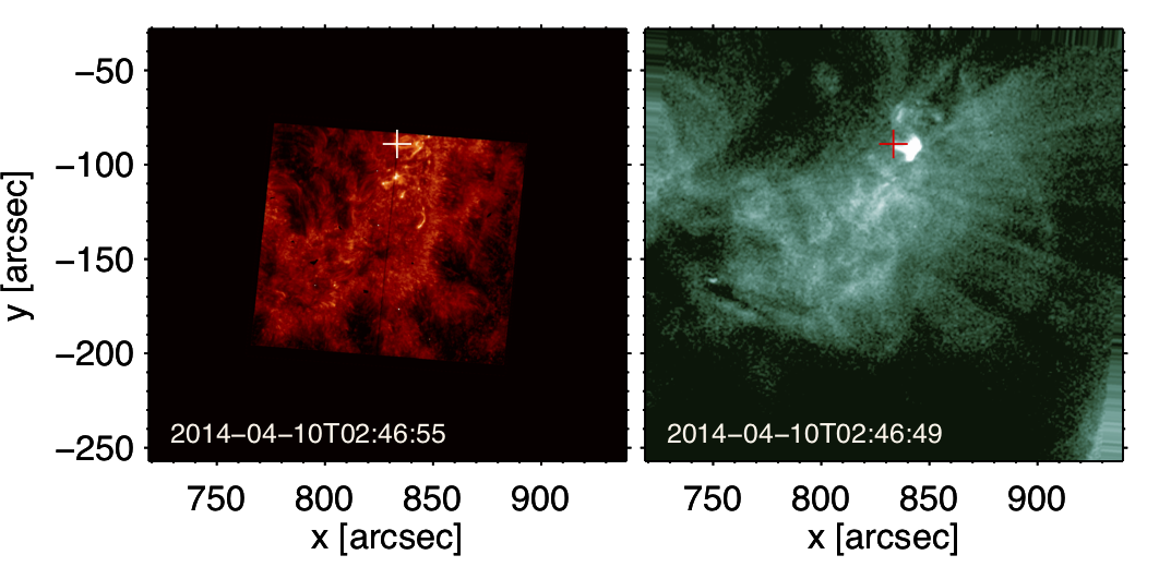
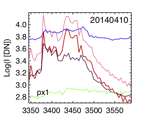
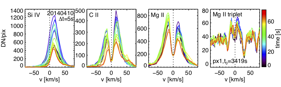
Figure 7: IRIS 1400Å slit-jaw images (top left) and AIA 94Å images (top right) showing a moss brightening event observed on 2014-04-10 (event 2 in Table 1), and associated hot loop emission. For the pixel marked in the images, we show the temporal evolution of IRIS spectral observables (lightcurves and spectra of different spectral lines). Figures are in the same format as Fig.1 and  2.

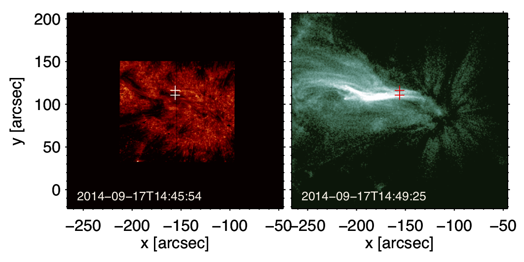
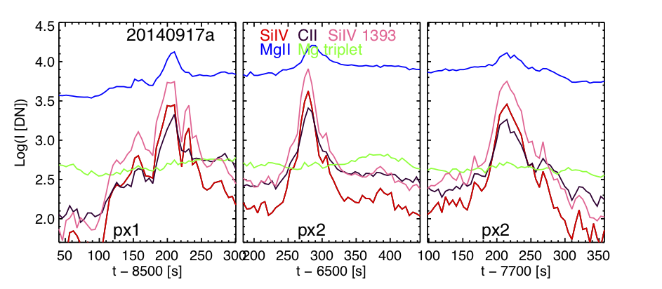
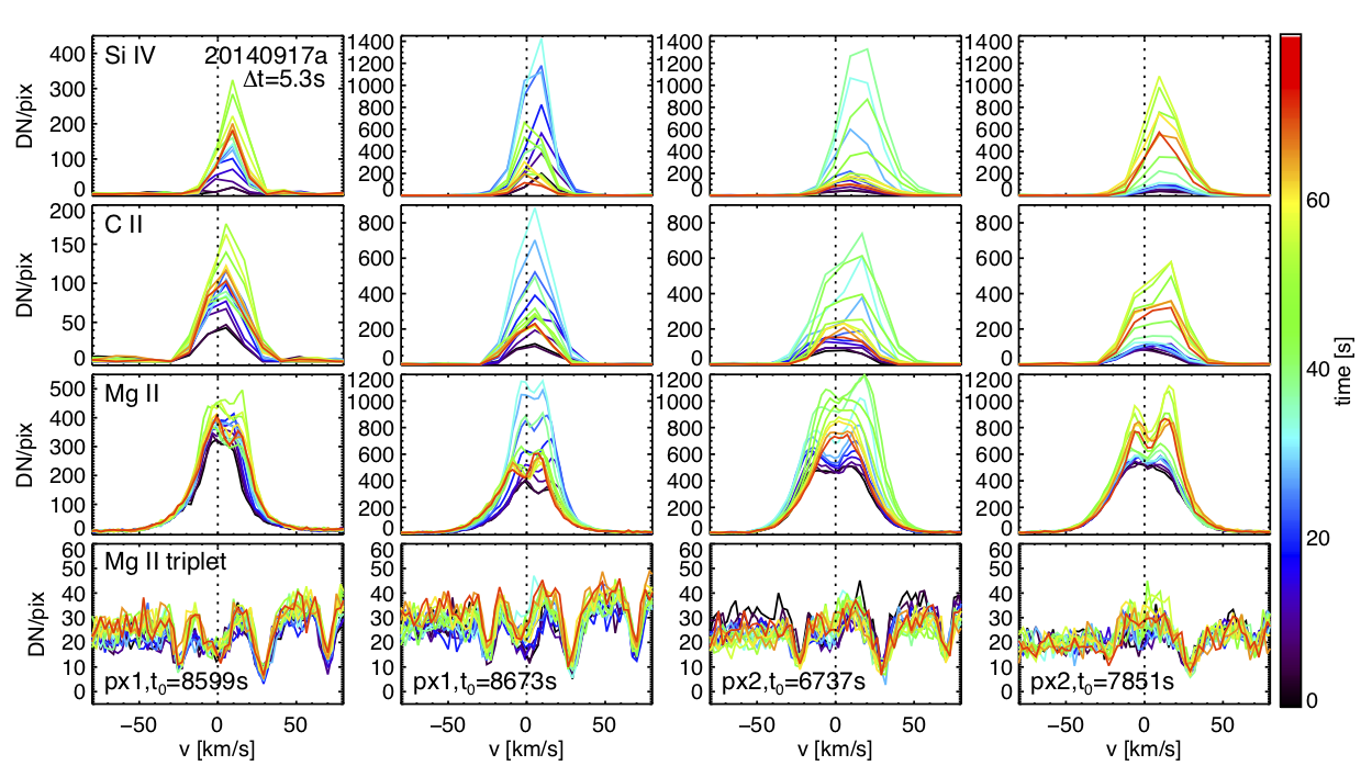
Figure 8: IRIS 1400Å slit-jaw images (top left) and AIA 94Å images (top right) showing moss brightenings observed on 2014-09-17 (event 3 in Table 1), and associated hot loop emission. For the 3 pixels marked in the images, we show (ordered by increasing value of solar y) the temporal evolution of IRIS spectral observables (lightcurves – second row – and spectra – bottom four rows – of different spectral lines). Figures are in the same format as Fig.1 and  2.

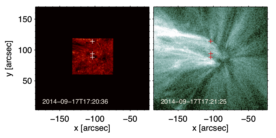
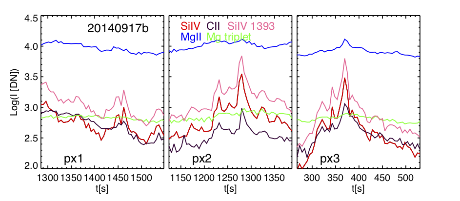
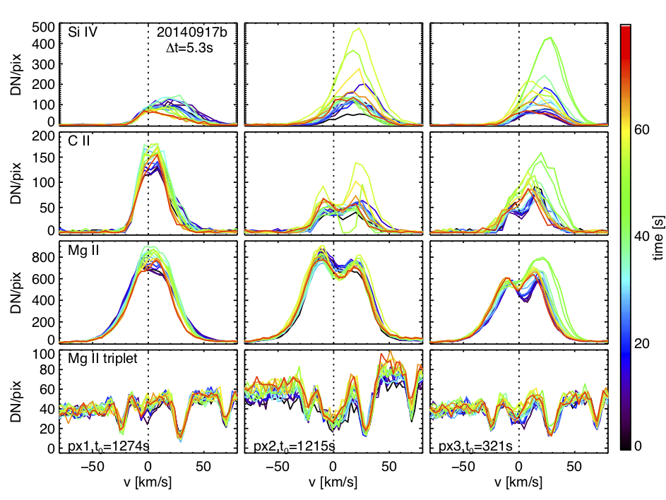
Figure 9: IRIS 1400Å slit-jaw images (top left) and AIA 94Å images (top right) showing moss brightenings observed on 2014-09-17 (event 4 in Table 1; in the same AR, and a few hours later, as event 3 shown in Fig. 8), and associated hot loop emission. For the 3 pixels marked in the images, we show (ordered by increasing value of solar y) the temporal evolution of IRIS spectral observables (lightcurves – second row – and spectra – bottom four rows – of different spectral lines). Figures are in the same format as Fig.1 and  2.

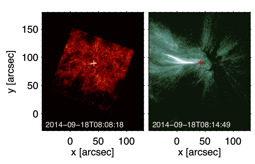
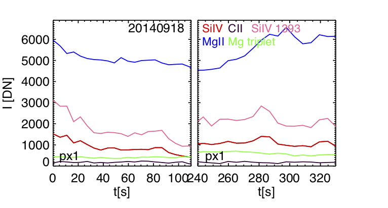
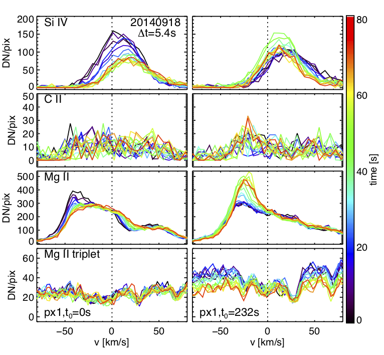
Figure 10: IRIS 1400Å slit-jaw images (top left) and AIA 94Å images (top right) showing moss brightenings event observed on 2014-09-18 (event 5 in Table 1), and associated hot loop emission. For the pixel marked in the images, we show (for 2 moss brightening events occurring at different times) the temporal evolution of IRIS spectral observables (lightcurves – second row – and spectra – bottom four rows – of different spectral lines). Figures are in the same format as Fig.1 and  2.

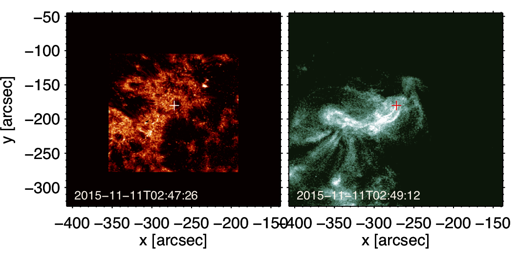
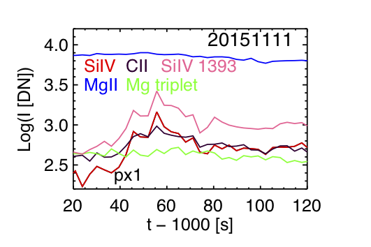
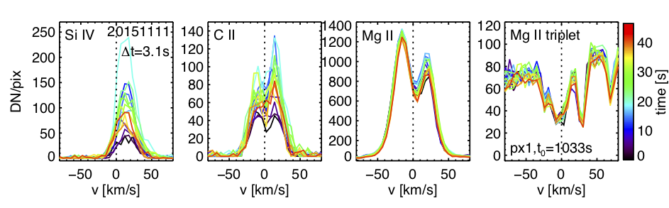
Figure 11: IRIS 1400Å slit-jaw images (top left) and AIA 94Å images (top right) showing moss brightenings event observed on 2015-11-11 (event 7 in Table 1), and associated hot loop emission. For the pixel marked in the images, we show the temporal evolution of IRIS spectral observables (lightcurves – second row – and spectra – bottom four rows – of different spectral lines). Figures are in the same format as Fig.1 and  2.

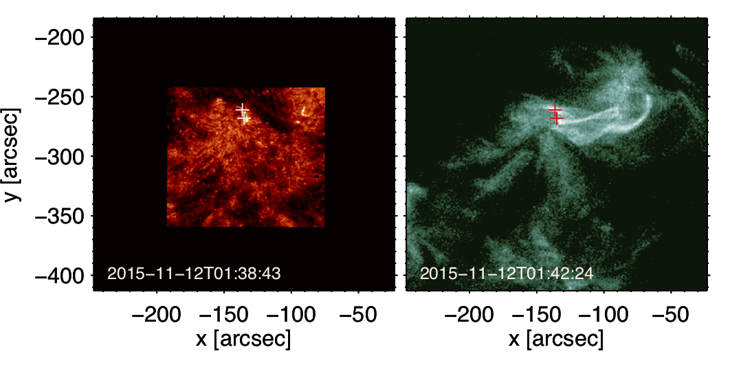
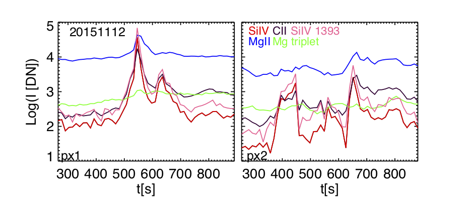
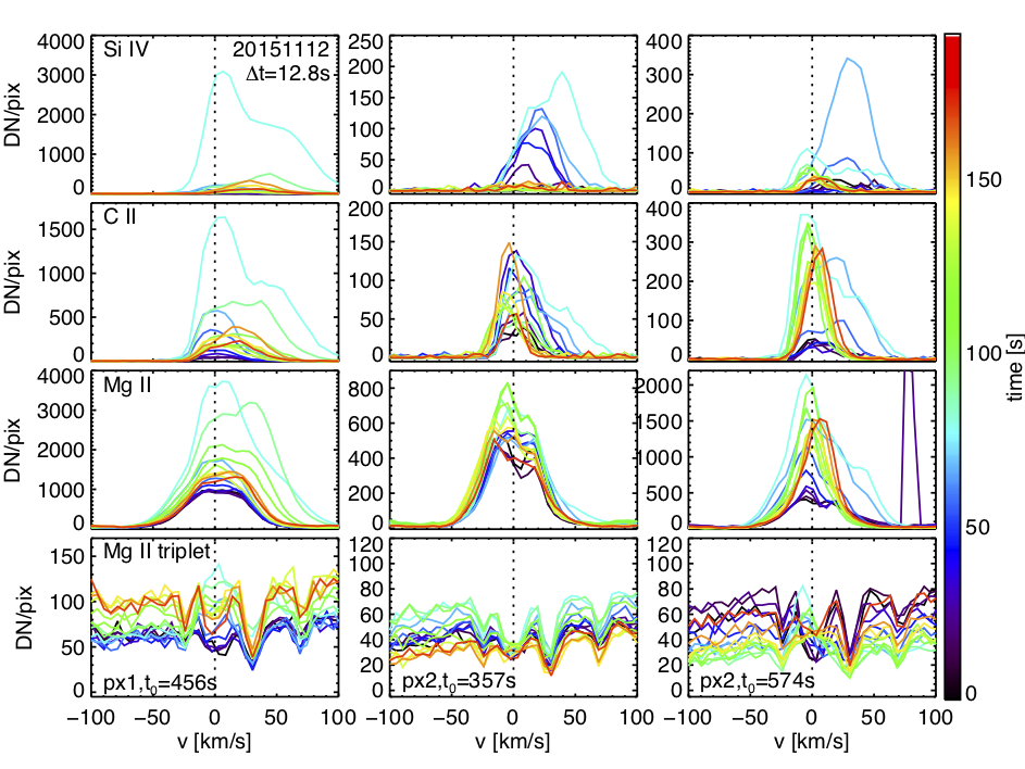
Figure 12: IRIS 1400Å slit-jaw images (top left) and AIA 94Å images (top right) showing moss brightenings observed on 2015-11-12 (event 8 in Table 1), and associated hot loop emission. For the 2 pixels marked in the images, we show (ordered by increasing value of solar y, and time of occurrence of event) the temporal evolution of IRIS spectral observables (lightcurves – second row – and spectra – bottom four rows – of different spectral lines). Figures are in the same format as Fig.1 and  2.

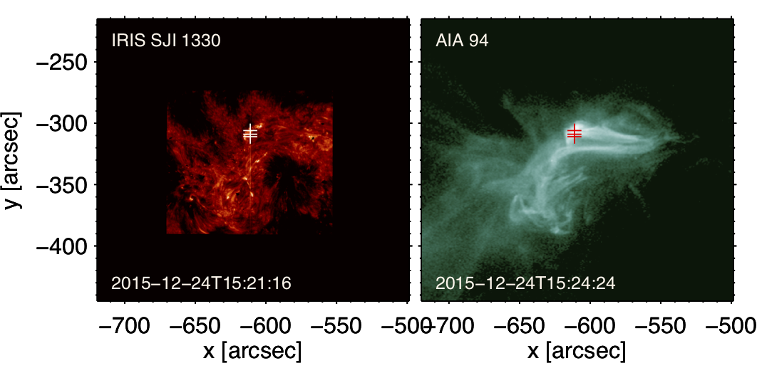
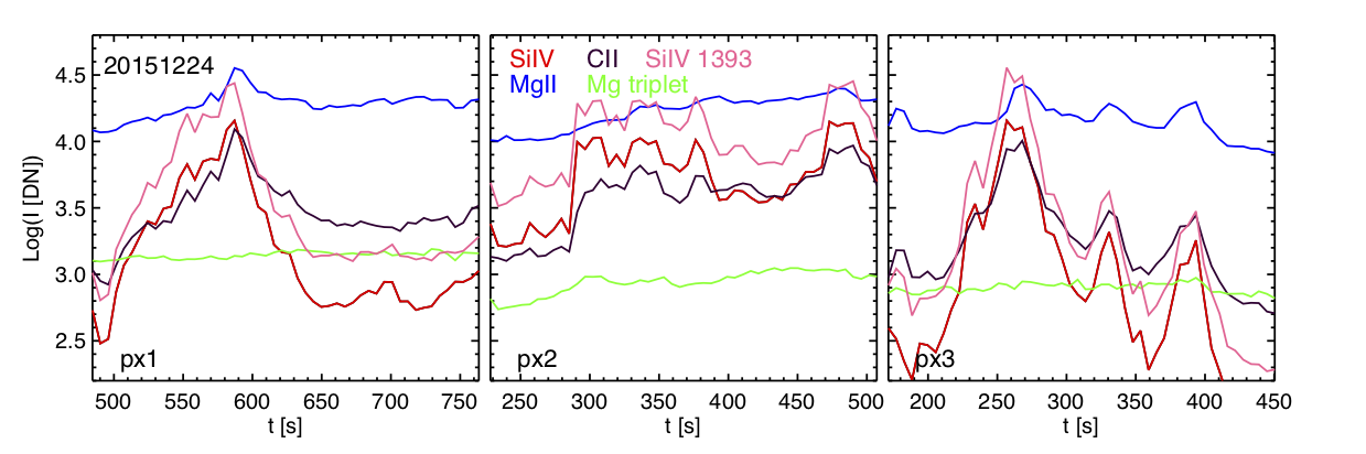
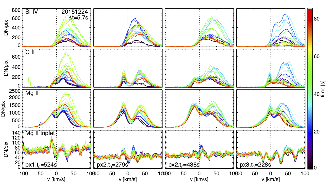
Figure 13: IRIS 1400Å slit-jaw images (top left) and AIA 94Å images (top right) showing moss brightenings observed on 2015-12-24 (event 9 in Table 1), and associated hot loop emission. For the 3 pixels marked in the images, we show (ordered by increasing value of solar y) the temporal evolution of IRIS spectral observables (lightcurves – second row – and spectra – bottom four rows – of different spectral lines). Figures are in the same format as Fig.1 and  2.

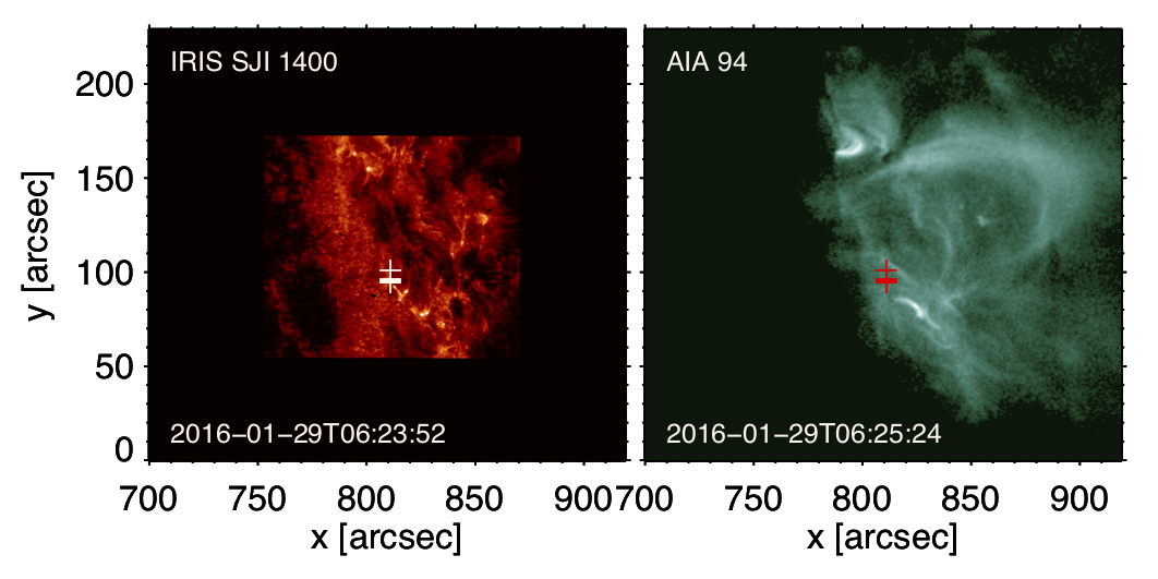
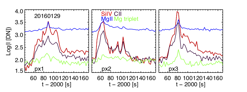
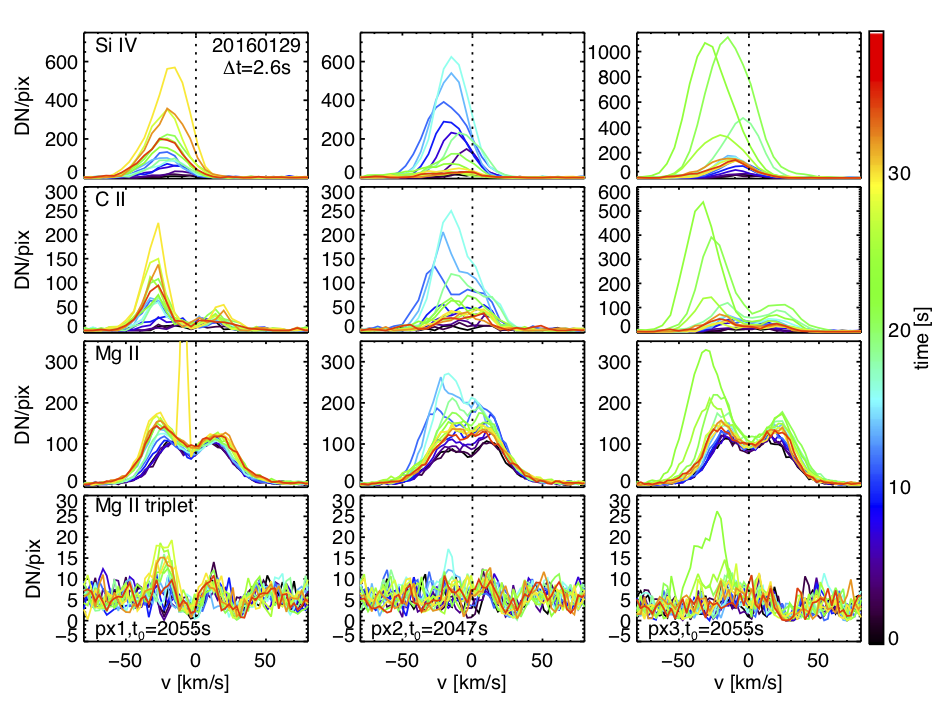
Figure 14: IRIS 1400Å slit-jaw images (top left) and AIA 94Å images (top right) showing moss brightenings observed on 2016-01-29 (event 10 in Table 1), and associated hot loop emission. For the 3 pixels marked in the images, we show (ordered by increasing value of solar y) the temporal evolution of IRIS spectral observables (lightcurves – second row – and spectra – bottom four rows – of different spectral lines). Figures are in the same format as Fig.1 and  2.

References

- Allred et al. (2005) Allred, J. C., Hawley, S. L., Abbett, W. P., & Carlsson, M. 2005, ApJ, 630, 573
- Allred et al. (2015) Allred, J. C., Kowalski, A. F., & Carlsson, M. 2015, ApJ, 809, 104
- Antiochos et al. (2003) Antiochos, S. K., Karpen, J. T., DeLuca, E. E., Golub, L., & Hamilton, P. 2003, ApJ, 590, 547
- Asgari-Targhi et al. (2019) Asgari-Targhi, M., van Ballegooijen, A. A., & Davey, A. R. 2019, ApJ, 881, 107
- Baker et al. (2015) Baker, D., Brooks, D. H., Démoulin, P., et al. 2015, ApJ, 802, 104
- Baker et al. (2018) Baker, D., Brooks, D. H., van Driel-Gesztelyi, L., et al. 2018, ApJ, 856, 71
- Barnes et al. (2019) Barnes, W. T., Bradshaw, S. J., & Viall, N. M. 2019, ApJ, 880, 56
- Berger et al. (1999) Berger, T. E., De Pontieu, B., Schrijver, C. J., & Title, A. M. 1999, ApJ, 519, L97
- Boerner et al. (2012) Boerner, P., Edwards, C., Lemen, J., et al. 2012, Sol. Phys., 275, 41
- Boerner et al. (2014) Boerner, P. F., Testa, P., Warren, H., Weber, M. A., & Schrijver, C. J. 2014, Sol. Phys., 289, 2377
- Bradshaw et al. (2012) Bradshaw, S. J., Klimchuk, J. A., & Reep, J. W. 2012, ApJ, 758, 53
- Brooks et al. (2009) Brooks, D. H., Warren, H. P., Williams, D. R., & Watanabe, T. 2009, ApJ, 705, 1522
- Brosius et al. (2014) Brosius, J. W., Daw, A. N., & Rabin, D. M. 2014, ApJ, 790, 112
- Bryans et al. (2016) Bryans, P., McIntosh, S. W., De Moortel, I., & De Pontieu, B. 2016, ApJ, 829, L18
- Cargill (1996) Cargill, P. J. 1996, Sol. Phys., 167, 267
- Cargill & Klimchuk (2004) Cargill, P. J., & Klimchuk, J. A. 2004, ApJ, 605, 911
- Cargill et al. (2015) Cargill, P. J., Warren, H. P., & Bradshaw, S. J. 2015, Philosophical Transactions of the Royal Society of London Series A, 373, 20140260
- Carlsson et al. (2015) Carlsson, M., Leenaarts, J., & De Pontieu, B. 2015, ApJ, 809, L30
- Carlsson & Stein (1997) Carlsson, M., & Stein, R. F. 1997, Chromospheric Dynamics - What Can Be Learnt from Numerical Simulations, ed. G. M. Simnett, C. E. Alissandrakis, & L. Vlahos, Vol. 489, 159
- Cheung et al. (2015) Cheung, M. C. M., Boerner, P., Schrijver, C. J., et al. 2015, ApJ, 807, 143
- Courrier et al. (2018) Courrier, H., Kankelborg, C., De Pontieu, B., & Wülser, J.-P. 2018, Sol. Phys., 293, 125
- De Pontieu et al. (2017) De Pontieu, B., Martínez-Sykora, J., & Chintzoglou, G. 2017, ApJ, 849, L7
- De Pontieu & McIntosh (2010) De Pontieu, B., & McIntosh, S. W. 2010, ApJ, 722, 1013
- De Pontieu et al. (2009) De Pontieu, B., McIntosh, S. W., Hansteen, V. H., & Schrijver, C. J. 2009, ApJ, 701, L1
- De Pontieu et al. (2014) De Pontieu, B., Title, A. M., Lemen, J. R., et al. 2014, Sol. Phys., 289, 2733
- Del Zanna et al. (2015a) Del Zanna, G., Dere, K. P., Young, P. R., Landi, E., & Mason, H. E. 2015a, A&A, 582, A56
- Del Zanna et al. (2015b) Del Zanna, G., Tripathi, D., Mason, H., Subramanian, S., & O’Dwyer, B. 2015b, A&A, 573, A104
- Dere et al. (1997) Dere, K. P., Landi, E., Mason, H. E., Monsignori Fossi, B. C., & Young, P. R. 1997, A&AS, 125, 149
- Edlén (1943) Edlén, B. 1943, ZAp, 22, 30
- Feldman (1992) Feldman, U. 1992, Phys. Scr, 46, 202
- Fletcher & De Pontieu (1999) Fletcher, L., & De Pontieu, B. 1999, ApJ, 520, L135
- Freeland & Handy (1998) Freeland, S. L., & Handy, B. N. 1998, Sol. Phys., 182, 497
- Galsgaard & Nordlund (1996) Galsgaard, K., & Nordlund, Å. 1996, J. Geophys. Res., 101, 13445
- Glesener et al. (2017) Glesener, L., Krucker, S., Hannah, I. G., et al. 2017, ApJ, 845, 122
- Graham et al. (2019) Graham, D. R., De Pontieu, B., & Testa, P. 2019, ApJ, 880, L12
- Grefenstette et al. (2016) Grefenstette, B. W., Glesener, L., Krucker, S., et al. 2016, ApJ, 826, 20
- Grotrian (1939) Grotrian, W. 1939, Naturwissenschaften, 27, 214
- Gudiksen & Nordlund (2005) Gudiksen, B. V., & Nordlund, Å. 2005, ApJ, 618, 1020
- Hannah et al. (2008) Hannah, I. G., Christe, S., Krucker, S., et al. 2008, ApJ, 677, 704
- Hannah et al. (2019) Hannah, I. G., Kleint, L., Krucker, S., et al. 2019, ApJ, 881, 109
- Hannah et al. (2016) Hannah, I. G., Grefenstette, B. W., Smith, D. M., et al. 2016, ApJ, 820, L14
- Hansteen et al. (2015) Hansteen, V., Guerreiro, N., De Pontieu, B., & Carlsson, M. 2015, ApJ, 811, 106
- Harrison et al. (2013) Harrison, F. A., Craig, W. W., Christensen, F. E., et al. 2013, ApJ, 770, 103
- Ishikawa & Krucker (2019) Ishikawa, S.-n., & Krucker, S. 2019, ApJ, 876, 111
- Ishikawa et al. (2014) Ishikawa, S.-n., Glesener, L., Christe, S., et al. 2014, PASJ, 66, S15
- Judge et al. (2017) Judge, P. G., Paraschiv, A., Lacatus, D., Donea, A., & Lindsey, C. 2017, ApJ, 838, 138
- Kerr et al. (2016) Kerr, G. S., Fletcher, L., Russell, A. e. J. B., & Allred, J. C. 2016, ApJ, 827, 101
- Klimchuk (2006) Klimchuk, J. A. 2006, Sol. Phys., 234, 41
- Klimchuk (2015) —. 2015, Philosophical Transactions of the Royal Society of London Series A, 373, 20140256
- Klimchuk & Cargill (2001) Klimchuk, J. A., & Cargill, P. J. 2001, ApJ, 553, 440
- Ko et al. (2009) Ko, Y., Doschek, G. A., Warren, H. P., & Young, P. R. 2009, ApJ, 697, 1956
- Kobayashi et al. (2014) Kobayashi, K., Cirtain, J., Winebarger, A. R., et al. 2014, Sol. Phys., 289, 4393
- Landi et al. (2012) Landi, E., Del Zanna, G., Young, P. R., Dere, K. P., & Mason, H. E. 2012, ApJ, 744, 99
- Lemen et al. (2012) Lemen, J. R., Title, A. M., Akin, D. J., et al. 2012, Sol. Phys., 275, 17
- Lin et al. (2002) Lin, R. P., Dennis, B. R., Hurford, G. J., et al. 2002, Sol. Phys., 210, 3
- Martínez-Sykora et al. (2018) Martínez-Sykora, J., De Pontieu, B., De Moortel, I., Hansteen, V. H., & Carlsson, M. 2018, ApJ, 860, 116
- Martínez-Sykora et al. (2017) Martínez-Sykora, J., De Pontieu, B., Hansteen, V. H., et al. 2017, Science, 356, 1269
- McTiernan (2009) McTiernan, J. M. 2009, ApJ, 697, 94
- Osborne et al. (2019) Osborne, C. M. J., Armstrong, J. A., & Fletcher, L. 2019, ApJ, 873, 128
- Panos et al. (2018) Panos, B., Kleint, L., Huwyler, C., et al. 2018, ApJ, 861, 62
- Parenti et al. (2017) Parenti, S., del Zanna, G., Petralia, A., et al. 2017, ApJ, 846, 25
- Parker (1983) Parker, E. N. 1983, ApJ, 264, 642
- Parker (1988) —. 1988, ApJ, 330, 474
- Parnell & De Moortel (2012) Parnell, C. E., & De Moortel, I. 2012, Philosophical Transactions of the Royal Society of London Series A, 370, 3217
- Pereira et al. (2015) Pereira, T. M. D., Carlsson, M., De Pontieu, B., & Hansteen, V. 2015, ApJ, 806, 14
- Pereira & Uitenbroek (2015) Pereira, T. M. D., & Uitenbroek, H. 2015, A&A, 574, A3
- Pesnell et al. (2012) Pesnell, W. D., Thompson, B. J., Chamberlin, P. C., et al. 2012, Sol. Phys., 275, 3
- Polito et al. (2018) Polito, V., Testa, P., Allred, J., et al. 2018, ApJ, 856, 178
- Polito et al. (2019) Polito, V., Testa, P., & De Pontieu, B. 2019, ApJ, 879, L17
- Priest et al. (2002) Priest, E. R., Heyvaerts, J. F., & Title, A. M. 2002, ApJ, 576, 533
- Rathore & Carlsson (2015) Rathore, B., & Carlsson, M. 2015, ApJ, 811, 80
- Reale (2014) Reale, F. 2014, Living Reviews in Solar Physics, 11, 4
- Reale et al. (2009) Reale, F., Testa, P., Klimchuk, J. A., & Parenti, S. 2009, ApJ, 698, 756
- Reale et al. (2019a) Reale, F., Testa, P., Petralia, A., & Graham, D. R. 2019a, ApJ, 882, 7
- Reale et al. (2019b) Reale, F., Testa, P., Petralia, A., & Kolotkov, D. Y. 2019b, arXiv e-prints, arXiv:1909.02847
- Sainz Dalda et al. (2019) Sainz Dalda, A., de la Cruz Rodríguez, J., De Pontieu, B., & Gošić, M. 2019, ApJ, 875, L18
- Schmit et al. (2015) Schmit, D., Bryans, P., De Pontieu, B., et al. 2015, ApJ, 811, 127
- Testa (2010) Testa, P. 2010, Proceedings of the National Academy of Science, 107, 7158
- Testa et al. (2016) Testa, P., De Pontieu, B., & Hansteen, V. 2016, ApJ, 827, 99
- Testa et al. (2012) Testa, P., De Pontieu, B., Martínez-Sykora, J., Hansteen, V., & Carlsson, M. 2012, ApJ, 758, 54
- Testa et al. (2005) Testa, P., Peres, G., & Reale, F. 2005, ApJ, 622, 695
- Testa & Reale (2012) Testa, P., & Reale, F. 2012, ApJ, 750, L10
- Testa et al. (2011) Testa, P., Reale, F., Landi, E., DeLuca, E. E., & Kashyap, V. 2011, ApJ, 728, 30
- Testa et al. (2015) Testa, P., Saar, S. H., & Drake, J. J. 2015, Philosophical Transactions of the Royal Society of London Series A, 373, 20140259
- Testa et al. (2013) Testa, P., De Pontieu, B., Martínez-Sykora, J., et al. 2013, ApJ, 770, L1
- Testa et al. (2014) Testa, P., De Pontieu, B., Allred, J., et al. 2014, Science, 346, B315
- Tripathi et al. (2010) Tripathi, D., Mason, H. E., Del Zanna, G., & Young, P. R. 2010, A&A, 518, A42
- Ugarte-Urra et al. (2019) Ugarte-Urra, I., Crump, N. A., Warren, H. P., & Wiegelmann, T. 2019, ApJ, 877, 129
- Ugarte-Urra & Warren (2012) Ugarte-Urra, I., & Warren, H. P. 2012, ApJ, 761, 21
- Ugarte-Urra & Warren (2014) —. 2014, ApJ, 783, 12
- Ugarte-Urra et al. (2017) Ugarte-Urra, I., Warren, H. P., Upton, L. A., & Young, P. R. 2017, ApJ, 846, 165
- van Ballegooijen et al. (2011) van Ballegooijen, A. A., Asgari-Targhi, M., Cranmer, S. R., & DeLuca, E. E. 2011, ApJ, 736, 3
- van Ballegooijen et al. (2017) van Ballegooijen, A. A., Asgari-Targhi, M., & Voss, A. 2017, ApJ, 849, 46
- Viall & Klimchuk (2011) Viall, N. M., & Klimchuk, J. A. 2011, ApJ, 738, 24
- Warren et al. (2016) Warren, H. P., Brooks, D. H., Doschek, G. A., & Feldman, U. 2016, ApJ, 824, 56
- Warren et al. (2012) Warren, H. P., Winebarger, A. R., & Brooks, D. H. 2012, ApJ, 759, 141
- Warren et al. (2008) Warren, H. P., Winebarger, A. R., Mariska, J. T., Doschek, G. A., & Hara, H. 2008, ApJ, 677, 1395
- Winebarger et al. (2018) Winebarger, A. R., Lionello, R., Downs, C., Mikić, Z., & Linker, J. 2018, ApJ, 865, 111
- Wright et al. (2017) Wright, P. J., Hannah, I. G., Grefenstette, B. W., et al. 2017, ApJ, 844, 132