Kernel density estimation based sampling for imbalanced class distribution

Abstract.

Imbalanced response variable distribution is a common occurrence in data science. In fields such as fraud detection, medical diagnostics, system intrusion detection and many others where abnormal behavior is rarely observed the data under study often features disproportionate target class distribution. One common way to combat class imbalance is through resampling the minority class to achieve a more balanced distribution. In this paper, we investigate the performance of the sampling method based on kernel density estimation (KDE). We believe that KDE offers a more natural way of generating new instances of minority class that is less prone to overfitting than other standard sampling techniques. It is based on a well established theory of nonparametric statistical estimation. Numerical experiments show that KDE can outperform other sampling techniques on a range of real life datasets as measured by $F_{1}$-score and G-mean. The results remain consistent across a number of classification algorithms used in the experiments. Furthermore, the proposed method outperforms the benchmark methods irregardless of the class distribution ratio. We conclude, based on the solid theoretical foundation and strong experimental results, that the proposed method would be a valuable tool in problems involving imbalanced class distribution.

1. Introduction

Imbalanced class distribution is a challenge that arises in many real world applications. It is prevalent in the fields of medical diagnostics, fraud detection, network intrusion detection and many others involving rare events [18]. Imbalanced class distribution usually appears in the context of a binary classification problem, where the response (target) variable consists of two classes with members of the majority class vastly outnumbering the members of the minority class. The majority and minority class members are labeled as negative and positive respectively. In such cases, learning models tend to be biased in favor of the negatively labeled class. Concretely, a classifier trying to minimize its prediction error rate would focus more on the negatively labeled instances as they comprise the majority of the data. At the same time, the positively labeled instances are often of more importance. For example, in medical diagnostics it would be critical to correctly identify patients with cancer though there may be relatively few such cases among the general population.

To combat the problem of class imbalance researchers have proposed various strategies [8, 20] that can generally be divided into four categories: resampling, cost-sensitive learning, one class learning, and feature selection. Resampling involves balancing the class distribution by either undersampling the majority class or oversampling the minority class. This is a very popular approach that has been shown to perform well in various scenarios [13, 23]. However, it is not without its limitations. Undersampling may lead to loss of potentially valuable information while oversampling may lead to overfitting. Cost sensitive learning is based on the idea of increasing the penalty for misclassifying the minority class instances. Since a classifier’s objective is to minimize the overall cost there will be greater emphasis put on instances of minority class [11, 17]. One class learning involves training a classifier on data with the target variable restricted to a single class. By ignoring all the majority class examples the classifier can get a clearer picture about the minority class [29]. Feature selection methods attempt to identify features that are effective in identifying minority class instances. This approach is particularly effective in cases involving high dimensional datasets [9, 24]. Ensemble techniques that combine two or more techniques described above have also been explored in the literature. One common approach is to combine feature selection and oversampling to handle imbalanced data [3, 34].

In this paper, we propose a sampling approach based on kernel density estimation to deal with imbalanced class distribution. Kernel density estimation is a well-known method for estimating the unknown probability density distribution based on a given sample [30, 32]. It estimates the unknown density function by averaging over a set of kernel homogeneous functions that are centered at each sample point. After having estimated the density distribution of the minority class we can then generate new sample points based on the density function. The proposed technique offers an intelligent and effective approach to synthesize new instances based on well-grounded statistical theory. Numerical experiments show that our method can perform better than other existing resampling techniques such as random sampling, SMOTE [4, 26], ADASYN [28], and NearMiss [25]. The paper is organized as follows. In Section 2, we give an overview of the relevant literature for our study. In Section 3, we describe the methodology used in the study. We present our results in Section 4, and Section 5 concludes the paper.

2. Literature

The problem of class imbalance arises in a number of real-life applications and various approaches to address this issue have been put forth by researchers. Krawczyk [18] presents a good overview of the current trends in the field. One of the common ways to tackle class imbalance is through resampling whereby the majority class is undersampled and/or the minority class is oversampled. In the former, a portion of the majority class instances is sampled according to some strategy to achieve a more balanced class distribution. Similarly, in the later approach the minority class is repeatedly sampled to increase its proportion relative to the majority class. One of the more popular undesampling techniques is NearMiss [25], where the negative samples are selected so that the average distance to the $k$ closest samples of the positive class is the smallest. In a slightly different variation of NearMiss those negative samples are selected for which the average distance to the $k$ farthest samples of the positive class is the smallest. As shown by Liu et al. [21, 22] an informed undersampling technique can lead to good results. However, in general, undesampling inevitably leads to loss of information. On the other hand, random sampling of the minority class (with replacement) can also cause issues such as overfitting [4]. More advanced sampling techniques attempt to overcome the issue of overfitting by generating new samples of the minority class in a more intelligent manner. In this regard, Chawla et al. [4] proposed a popular oversampling technique called SMOTE. In their approach, new instances are generated by random linear interpolation between the existing minority samples. Given a minority sample point $P_{0}$ a new random point is chosen along the line segment joining $P_{0}$ to one of its nearest neighbors $P_{i}$. This method has proven to be effective in a number of applications [6]. Another popular variant of SMOTE is an adaptive algorithm called ADASYN [10, 28]. It creates more examples in the neighborhood of the boundary between the two classes than in the interior of the minority class. There also exist nonlinear variants of SMOTE such as [26], where the authors interpolate between the points in the feature space of kernel SVM. An oversampling method based on Mahalanobis distance was proposed in [1]. The authors propose to generate new samples of the minority class that have the same Mahalanobis distance from the class mean as the existing minority points. Experiments showed that the method performs well on multi-class imbalanced data. An intelligent combination of undersampling and oversampling techniques may also be an interesting avenue of study as was argued by the authors in [13].

The sampling technique proposed in this paper relies on approximating the underlying density distribution of the minority class based on the existing samples. Probability density estimation techniques can be categorized into two groups: parametric and nonparametric. In parametric methods a fixed density function is assumed and its parameters are then estimated by maximizing the likelihood of obtaining the current sample. This approach introduces a specification bias and is susceptible to ovefitting [19]. Nonparametric approaches estimate the density distribution directly from the data. Among the nonparametric methods kernel density estimation (KDE) is the most popular approach in the literature [32, 33]. It is a well established technique both within the statistical and machine learning communities [2, 16]. KDE has been successfully used in a wide array of applications including breast cancer data analysis [31], image annotation [35], wind power forecast [12], and outlier detection [15].

A KDE based sampling approach was used in [7], where the authors applied a 2-step procedure by first oversampling the minority samples using KDE and then constructing a radial basis function classifier. Numerical experiments on 6 datasets showed that their method performed better than comparable techniques. Our paper differs from [7] in that we perform a systematic study of the KDE method. We delve deeper to analyze the differences between KDE and other sampling techniques. We carry out a large number of numerical experiments to compare the performance of KDE to other standard sampling methods.

3. KDE sampling

Nonparametric density estimation is an important tool in statistical data analysis. It is used to model the distribution of a variable based on a random sample. The resulting density function can be utilized to investigate various properties of the variable. Let $\{x_{1},x_{2},...,x_{n}\}$ be an i.i.d. sample drawn from an unknown probability density function $f$. Then the kernel density estimate of $f$ is given by

(1) $$\tilde{f}(x)=\frac{1}{n}\sum_{i=1}^{n}K_{h}(x-x_{i}),$$

where $K$ is the kernel function, $h$ is the bandwidth parameter, and $K_{h}(t)=\frac{1}{h}K(\frac{t}{h})$. Intuitively, the true value of $f(x)$ is estimated as the average distance from $x$ to the sample data points $x_{i}$. The ’distance’ between $x$ and $x_{i}$ is calculated via a kernel function $K(t)$. There exists a number of kernel functions that can be used for this purpose including Epanechnikov, exponential, tophat, linear, and cosine. However, the most popular kernel is the Gaussian function i.e.

(2) $$K(t)=\phi(t),$$

where $\phi$ is the standard normal density distribution. The bandwidth parameter $h$ controls the smoothness of the density function estimate as well as the tradeoff between the bias and variance. A large value of $h$ results in a very smooth (low variance), but high bias density distribution. A small value of $h$ leads to an unsmooth (high variance), but low bias density distribution. The value of $h$ has a much bigger effect on the KDE approximation than the actual kernel. The value of $h$ can be determined by optimizing the mean integrated square error:

(3) $$\mbox{MISE}(h)=E\big{[}\int(\tilde{f}(x)-f(x))^{2}\,dx\big{]}.$$

The MISE formula cannot be used directly since it involves the unknown density function $f$. Therefore, a number of other methods have been developed to determine the optimal value of $h$. The two most frequently used approaches to select the bandwidth value are rule of thumb methods and cross-validation. The rule of thumb methods approximate the optimal value of $h$ under certain assumptions about the underlying density function $f$ and its estimate $\tilde{f}$. A common approach is to use Scott’s rule of thumb [30] for the value of $h$:

(4) $$h=n^{-\frac{1}{5}}\cdot s,$$

where $s$ is the sample standard deviation. The optimal bandwidth value can also be determined numerically through cross-validation. It is done by applying a grid search method to find the value of $h$ that minimizes the sample mean integrated square error:

(5) $$\mbox{MISE}_{n}(h)=\frac{1}{n}\sum_{i=1}^{n}(\tilde{f}(x_{i})-f(x_{i}))^{2}.$$

Kernel density estimation for multivariate variables follows essentially the same approach as the one dimensional approach described above. Given a sample $\{\boldsymbol{x}_{1},\boldsymbol{x}_{2},...\boldsymbol{x}_{n}\}$ of $d$-dimensional random sample vectors drawn from a distribution described by a density function $f$ the kernel density estimate is defined to be

(6) $$\boldsymbol{\tilde{f}_{H}(x)}=\frac{1}{n}\sum_{i=1}^{n}\boldsymbol{K_{H}(x-x_{i})},$$

where $\boldsymbol{H}$ is a $d\times d$ bandwidth matrix. The bandwidth matrix can be chosen in a variety of ways. In this study, we use the multivariate version of Scott’s rule:

(7) $$\boldsymbol{H}=n^{-\frac{1}{d+4}}\cdot\boldsymbol{S},$$

where $\boldsymbol{S}$ is a the data covariance matrix. Furthermore, we use multivariate normal distribution as the kernel function:

(8) $$\boldsymbol{K_{H}(x)}=\frac{1}{\sqrt{(2\pi)^{d}|\boldsymbol{H}|}}e^{-\frac{1}{2}\boldsymbol{x^{T}H^{-1}x}}.$$

The difference between KDE sampling and other standard sampling methods is illustrated in Figure 1. The original data in the figure consists of 100 uniformly distributed blue points with the points in radius of 2 from the center being dropped. The 25 orange points are generated in the center of the figure via Gaussian distribution with standard deviation of 2. As can be seen from the figure, KDE creates new sample points by ’spraying’ around the existing minority class points. The points are created using Gaussian distribution centered at randomly chosen existing minority class points. This process seems more intuitive than other sampling methods. On other hand, SMOTE method creates new sample points by interpolating between the existing minority class points. As a result all SMOTE generated points lie in the convex hull of the original minority class samples. Therefore, the new sampled data does not represent well the true underlying population distribution. Random sampling with replacement (ROS) creates new points by simply resampling the existing minority class points. As a result the new sampled data differs very little from the original data though it is more dense at each sample location. ADASYN sampled plot resembles the SMOTE plot but creates a bigger number of points at the edge of the minority cluster. NearMiss undersamples from the majority class thereby losing a lot of information as can be seen from its plot.

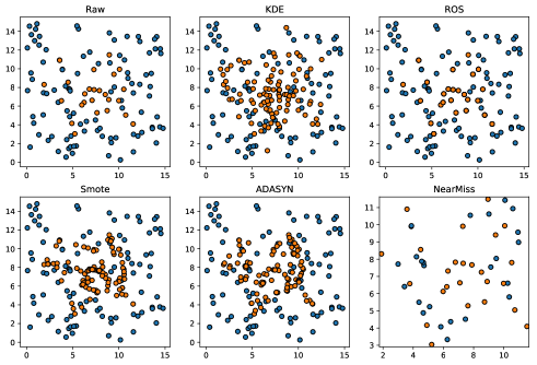
Figure 1. Resampled data based on various techniques.

4. Numerical Experiments

In this section, we carry out a number of experiments to evaluate the performance of the KDE sampling method. To this end, we compare KDE to four standard sampling approaches used in the literature: Random Oversampling (ROS), SMOTE, ADASYN, and NearMiss. The ROS method is the simplest approach to generate additional minority class instances. Concretely, the new instances are randomly selected from the minority class with replacement. The ROS method serves as a basic benchmark for other sampling methods. The SMOTE algorithm is a widely used oversampling technique for generating new instances of the minority class [4]. Unlike ROS, the SMOTE algorithm creates new instances synthetically. Concretely, for each point in the minority class its $k$ nearest neighbors in the minority class are determined. Given a minority point and one of its neighbors, the difference between the two is calculated and multiplied by a random number between $0$ and $1$. The new minority class instance is obtained by adding the preceding result to the minority point:

(9) $$p^{-}_{new}=p^{-}+t(p^{-}-p^{-}_{k}),$$

where $p^{-}_{new}$ denotes the new minority class point, $p^{-}$ is the minority point under consideration, $p^{-}_{k}$ is a $k$th nearest neighbor, and $t$ is a random number between $0$ and $1$. Thus, the SMOTE algorithm creates new instances by linearly interpolating between $k$ nearest neighbors of minority class points. ADASYN is a popular extension of SMOTE [10]. It uses the same algorithm as SMOTE (Equation 9) to generate new instances of the minority class. However, ADASYN generates more points around the minority instances which are closer to the majority class. In particular, for each minority instance $p^{-}$, its $k$ nearest neighbors are determined and the learning difficulty rate is calculated according to:

(10) $$r=\frac{m}{k},$$

where $m$ is the number of majority class members in the $k$ nearest neighborhood. Consequently, ADASYN generates more points around the minority instances with higher $r$ values. NearMiss is a popular undersampling technique used to reduce the size of the majority class data [25]. It aims to sample instances of the majority class in a manner that preserves the original boundary structure of the data. There exist several variations of the NearMiss algorithm. In the most popular version the NearMiss algorithm, the majority class instances that are closest to the minority class are selected. To this end, pairwise distances between members of the majority and minority classes are calculated. Then for each point in the majority class $p^{+}$, the average distance to the closest $k$ points of the minority class $\overline{d}_{p^{+}}$ is calculated. The points $p^{+}$ with the corresponding smallest values of $\overline{d}_{p^{+}}$ are selected as the majority class sample.

The implementations of all four sampling approaches are taken from the imblearn Python library [20] with their default settings. The implementation of KDE is taken from scipy.stats Python library [14] with its default settings. In particular, we used the multivariate Gaussian KDE with its default bandwidth value determined by Scott’s Rule (see Equations 6 - 8). Note that the performance of the KDE method can be further optimized by choosing the bandwidth value via cross validation.

The usual measures of classifier performance such as the accuracy rate are not suitable in the context of imbalanced datasets because their results can be misleading. For instance, given a dataset with 90$\%$ of instances labeled as negative, we can achieve a 90$\%$ accuracy rate by simply guessing all the instances to be negative. Although we would obtain a high accuracy rate we would miss all the positive instances in the data. Ideally, we would like a metric that would measure classifier performance on both classes. To address this issue, authors often use the area under receiver operating characteristic curve (AUC) [4, 27]. AUC reflects classifier performance based on true positive and false positive rates and it is not sensitive to class imbalance [5]. However, calculating AUC requires probabilities of the predicted labels which are not readily available for certain algorithms including KNN and SVM. Therefore, as an alternative to AUC, we also use G-mean:

(11) $$\mbox{G-mean}=\sqrt{\frac{TP}{TP+FN}\cdot\frac{TN}{TN+FP}}$$

and $F_{1}$-score:

(12) $$F_{1}=2\cdot\frac{precision\cdot recall}{precision+recall}$$

to measure classifier performance [24, 27].

4.1. Simulated Data

We begin by considering a situation similar to the one described in Figure 1. We use a dataset of size 1000 where the majority class points are uniformly distributed over a square grid. Next, we remove the points within radius of 2 from the center from the majority set. The minority class points are simulated using Gaussian distribution with mean at the center of the grid and standard deviation of 2. We measure the performance of the sampling methods over a range of class imbalance ratios. We use a feedforward neural network with one hidden layer as our base classifier. The results of the experiment are presented in Figure 2. We see that the KDE sampling technique outperforms other methods as measured by G-mean and $F_{1}$-score. Moreover, KDE has the edge under different class imbalance ratios. As measured by AUC, KDE is the best at 80$\%$ imbalance ratio and second best at $70\%$ and $90\%$ imbalance ratios.

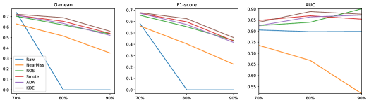
Figure 2. Performance of sampling method under varying class imbalance ratios.

Next, we consider a dataset consisting of 500 majority and 100 minority class instances. The sample points are generated using a uniform distribution. The data is constructed to be almost linearly separable (see Figure 3a). We apply various sampling techniques to the raw data with the results illustrated in Figures 3b-3f. As can be seen from the figures the new KDE minority samples are spread across a larger region. On the other hand, ROS, SMOTE, and ADASYN generated samples are more concentrated making them more prone to overfitting.

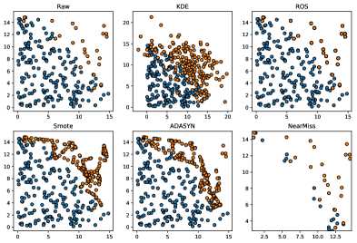
Figure 3. Resampled data for a nearly (linearly) separable data.

A feedfoward neural network is trained on each resampled dataset. The AUC results are presented in Table 1. As can be seen from the table, KDE significantly outperforms the other sampling techniques.

Table 1. AUC results for data in Figure 3.

Metric	Raw	NearMiss	ROS	SMOTE	ADASYN	KDE
AUC	0.757	0.727	0.820	0.8301	0.814	0.871

Our last illustration is in three-dimensional space as shown in Figure 4. The majority class samples consist of 500 uniformly distributed points over the cube $[0,15]^{3}$ with the sphere of radius 1.5 removed from the center of the set. The minority class samples consist of 100 points generated according to the Gaussian distribution with $\mu=(7,7,7)$ and $\sigma=2$. As can be seen from Figure 4, the KDE resampled data appears to be more diffused whereas ROS, SMOTE, and ADASYN generated data is more concentrated.

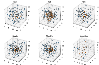
Figure 4. Generated samples in 3D.

A feedfoward neural network is trained on each resampled dataset and the results are presented in Table 2. As can be observed from the table, KDE achieves the best results in AUC and $F_{1}$-score. And it is second best in terms of G-mean.

Table 2. AUC results for data in Figure 4.

	Raw	NearMiss	ROS	SMOTE	ADASYN	KDE
AUC	0.870593	0.74237	0.883333	0.874519	0.862889	0.890148
G-mean	0.17598	0.554593	0.63151	0.602904	0.610252	0.618056
$F_{1}$-score	0.020202	0.403148	0.544493	0.511166	0.519447	0.546625

4.2. Real Life Data

In order to obtain a comprehensive evaluation of our method we used a range of datasets and classifiers. In particular, we used 12 real life datasets with various class imbalance ratios ranging from $1.86:1$ to $42:1$ (Table 3). Each sampling method is tested on 3 separate base classifiers: $k$-nearest neighbors (KNN), support vector machines (SVM), and multilayer perceptron (MLP).

Table 3. Experimental Datasets

	Name	Repository & Target	Ratio	#S	#F
1	diabetes	UCI, target: 1	1.86:1	768	8
2	bank	UCI, target: yes	7.6:1	43,193	24
3	ecoli	UCI, target: imU	8.6:1	336	7
4	satimage	UCI, target: 4	9.3:1	6,435	36
5	abalone	UCI, target: 7	9.7:1	4,177	10
6	spectrometer	UCI, target: $>$=44	11:1	531	93
7	yeast_ml8	LIBSVM, target: 8	13:1	2,417	103
8	scene	LIBSVM, target: $>$one label	13:1	2,407	294
9	libras_move	UCI, target: 1	14:1	360	90
10	wine_quality	UCI, wine, target: $<$=4	26:1	4,898	11
11	letter_img	UCI, target: Z	26:1	20,000	16
12	yeast_me2	UCI, target: ME2	28:1	1,484	8
13	ozone_level	UCI, ozone, data	34:1	2,536	72
14	mammography	UCI, target: minority	42:1	11,183	6

During the experiments the data was split into training and testing parts. The results based on the testing part are calculated and reported in the study. Furthermore, each experiment was run twice using different training/testing splits. The average value of the results of the two runs are being presented in the paper. The results for each classifier are summarized in 3 separate tables below. When using the KNN algorithm, the KDE sampling method often yields significantly better results compared to other sampling methods (see Table 4). For instance, when used on ecoli dataset the KDE method produces G-mean of 0.753 which is 5$\%$ better than the second best method (SMOTE); and $F_{1}$-score of 0.691 which is 6$\%$ better than the second best method. Note that the KDE method performs well on datasets with both low and high imbalance ratios.

Table 4. G-mean and $F_{1}$-score results based on KNN classifier.

	NearMiss	ROS	SMOTE	ADASYN	KDE
diabetes G	0.685	0.693	0.695	0.673	0.711
diabetes $F_{1}$	0.613	0.623	0.634	0.614	0.622
bank G	0.393	0.584	0.584	0.575	0.689
bank $F_{1}$	0.270	0.461	0.470	0.462	0.345
ecoli G	0.457	0.679	0.705	0.686	0.753
ecoli $F_{1}$	0.339	0.593	0.631	0.611	0.691
satimage G	0.352	0.715	0.670	0.653	0.732
satimage $F_{1}$	0.223	0.650	0.608	0.589	0.633
abalone G	0.200	0.478	0.470	0.478	0.492
abalone $F_{1}$	0.098	0.336	0.339	0.350	0.191
spectrometer G	0.641	0.936	0.890	0.915	0.961
spectrometer $F_{1}$	0.521	0.771	0.754	0.771	0.723
yeast_ml8 G	0.316	0.284	0.294	0.298	0.557
yeast_ml8 $F_{1}$	0.172	0.125	0.161	0.166	0.068
scene G	0.302	0.451	0.372	0.368	0.546
scene $F_{1}$	0.145	0.285	0.241	0.236	0.096
libras_move G	0.842	0.823	0.760	0.740	0.874
libras_move $F_{1}$	0.647	0.806	0.730	0.707	0.842
wine_quality G	0.270	0.456	0.393	0.395	0.527
wine_quality $F_{1}$	0.129	0.291	0.252	0.256	0.335
letter_img G	0.438	0.956	0.940	0.938	0.943
letter_img $F_{1}$	0.321	0.945	0.932	0.931	0.934
yeast_me2 G	0.300	0.458	0.488	0.475	0.465
yeast_me2 $F_{1}$	0.153	0.285	0.366	0.344	0.293
ozone_level G	0.134	0.390	0.335	0.348	0.374
ozone_level $F_{1}$	0.036	0.209	0.189	0.205	0.111
mammography G	0.179	0.666	0.567	0.522	0.663
mammography $F_{1}$	0.062	0.570	0.469	0.416	0.568

Applying SVM to compare the sampling methods produces results that are similar to KNN. As can be seen from Table 5, KDE often yields significantly better results than other sampling methods. For instance, when used on spectrometer dataset the KDE method produces G-mean of 0.924 which is 12$\%$ better than the second best method (SMOTE); and $F_{1}$-score of 0.878 which is 14$\%$ better than the second best method. Note again that the KDE method performs well on datasets with both low and high imbalance ratios.

Table 5. G-mean and $F_{1}$-score results based on SVM classifier.

	NearMiss	ROS	SMOTE	ADASYN	KDE
diabetes G	0.681	0.705	0.701	0.704	0.706
diabetes $F_{1}$	0.626	0.647	0.633	0.654	0.635
bank G	0.378	0.594	0.599	0.581	0.701
bank $F_{1}$	0.255	0.504	0.507	0.489	0.411
ecoli G	0.309	0.699	0.698	0.698	0.709
ecoli $F_{1}$	0.190	0.648	0.636	0.636	0.659
satimage G	0.327	0.652	0.663	0.612	0.618
satimage $F_{1}$	0.199	0.582	0.596	0.538	0.542
abalone G	0.184	0.494	0.492	0.485	0.508
abalone $F_{1}$	0.085	0.389	0.385	0.377	0.401
spectrometer G	0.555	0.795	0.808	0.802	0.924
spectrometer $F_{1}$	0.436	0.720	0.732	0.738	0.878
yeast_ml8 G	0.276	0.264	0.278	0.278	na
yeast_ml8 $F_{1}$	0.146	0.048	0.018	0.018	na
scene G	0.279	0.622	0.583	0.578	0.472
scene $F_{1}$	0.149	0.349	0.314	0.306	0.178
libras_move G	0.351	0.867	0.886	0.886	0.935
libras_move $F_{1}$	0.218	0.804	0.878	0.878	0.933
wine_quality G	0.235	0.404	0.413	0.405	0.440
wine_quality $F_{1}$	0.105	0.261	0.271	0.263	0.287
letter_img G	0.462	0.944	0.963	0.973	0.796
letter_img $F_{1}$	0.351	0.932	0.951	0.961	0.772
yeast_me2 G	0.217	0.430	0.456	0.443	0.504
yeast_me2 $F_{1}$	0.089	0.293	0.323	0.309	0.380
ozone_level G	0.146	0.446	0.451	0.436	0.426
ozone_level $F_{1}$	0.043	0.294	0.296	0.278	0.262
mammography G	0.191	0.517	0.553	0.472	0.535
mammography $F_{1}$	0.070	0.411	0.454	0.355	0.427

Using the MLP classifier does not produce as strong of results as using KNN or SVM. Although there are instances - ecoli, mammography - where KDE outperforms other sampling methods its performance is not overwhelming (see Table 6). This may be the result of the particular network architecture used in the experiment: a single hidden layer with 32 fully connected nodes. It is possible that a different architecture may produce better results for KDE sampling.

Table 6. G-mean and $F_{1}$-score results based on MLP classifier.

	NearMiss	ROS	SMOTE	ADASYN	KDE
diabetes G	0.712	0.725	0.715	0.702	0.695
diabetes $F_{1}$	0.659	0.665	0.645	0.644	0.628
bank G	0.388	0.607	0.614	0.589	0.721
bank $F_{1}$	0.266	0.519	0.525	0.498	0.377
ecoli G	0.390	0.741	0.765	0.724	0.762
ecoli $F_{1}$	0.263	0.688	0.708	0.667	0.724
satimage G	0.337	0.722	0.734	0.761	0.655
satimage $F_{1}$	0.209	0.648	0.652	0.674	0.555
abalone G	0.197	0.513	0.513	0.498	0.522
abalone $F_{1}$	0.097	0.407	0.405	0.388	0.253
spectrometer G	0.368	0.882	0.957	0.952	0.931
spectrometer $F_{1}$	0.239	0.715	0.700	0.758	0.741
yeast_ml8 G	0.279	0.324	0.381	0.462	0.313
yeast_ml8 $F_{1}$	0.147	0.098	0.115	0.188	0.082
scene G	0.311	0.537	0.504	0.516	0.466
scene $F_{1}$	0.178	0.261	0.246	0.268	0.202
libras_move G	0.379	0.956	0.913	0.963	0.958
libras_move $F_{1}$	0.250	0.845	0.813	0.883	0.890
wine_quality G	0.223	0.439	0.434	0.443	0.449
wine_quality $F_{1}$	0.096	0.289	0.289	0.298	0.299
letter_img G	0.593	0.980	0.971	0.971	0.882
letter_img $F_{1}$	0.517	0.964	0.954	0.948	0.873
yeast_me2 G	0.215	0.499	0.500	0.491	0.623
yeast_me2 $F_{1}$	0.089	0.370	0.362	0.357	0.317
ozone_level G	0.178	0.493	0.444	0.364	0.406
ozone_level $F_{1}$	0.062	0.257	0.237	0.166	0.171
mammography G	0.183	0.560	0.585	0.490	0.629
mammography $F_{1}$	0.065	0.467	0.497	0.378	0.518

5. Conclusion

In this paper, we studied an oversampling technique based on KDE. We believe that KDE provides a natural and statistically sound approach to generating new minority samples in an imbalanced dataset. It allows creation of new instances with minimum overfitting. One of the main advantages of KDE technique is its flexibility. By choosing different kernel functions researchers can customize the sampling process. Additional flexibility is offered through selection of the kernel bandwidth. KDE is a well researched topic with an established statistical foundation. In addition, a variety of implementations of the KDE algorithm are available in Python, R, Julia and other programming languages. This makes KDE a very appealing tool to use in oversampling.

We carried out a comprehensive study of the KDE sampling approach based on simulated and real life data. In particular, we used 3 simulated and 12 real life datasets that were tested on three different base classifiers. The proposed method was compared against four standard benchmark techniques for dealing with imbalanced class data. The results, as measured by $F_{1}$-score and G-mean, show that KDE has the ability to outperform other standard sampling methods in a number of different scenarios. The performance of KDE remains robust regardless of the base classifier used which indicates generalizability of the proposed method. Based on the above analysis, we conclude that KDE should be considered as a potent tool in dealing with the problem of imbalanced class distribution.

References

- [1] Abdi, L., and Hashemi, S. (2016). To combat multi-class imbalanced problems by means of over-sampling techniques. IEEE transactions on Knowledge and Data Engineering, 28(1), 238-251.
- [2] Botev, Z. I., Grotowski, J. F., and Kroese, D. P. (2010). Kernel density estimation via diffusion. The annals of Statistics, 38(5), 2916-2957.
- [3] Cao, P., Liu, X., Zhang, J., Zhao, D., Huang, M., & Zaiane, O. (2017). 2, 1 norm regularized multi-kernel based joint nonlinear feature selection and over-sampling for imbalanced data classification. Neurocomputing, 234, 38-57.
- [4] Chawla, N. V., Bowyer, K. W., Hall, L. O., and Kegelmeyer, W. P. (2002). SMOTE: synthetic minority over-sampling technique. Journal of artificial intelligence research, 16, 321-357.
- [5] Fawcett, T. (2006). An introduction to ROC analysis. Pattern recognition letters, 27(8), 861-874.
- [6] Fernández, A., Garcia, S., Herrera, F., Chawla, N. V. (2018). Smote for learning from imbalanced data: progress and challenges, marking the 15-year anniversary. Journal of artificial intelligence research, 61, 863-905.
- [7] Gao, M., Hong, X., Chen, S., Harris, C. J., Khalaf, E. (2014). PDFOS: PDF estimation based over-sampling for imbalanced two-class problems. Neurocomputing, 138, 248-259.
- [8] Haixiang, G., Yijing, L., Shang, J., Mingyun, G., Yuanyue, H., and Bing, G. (2017). Learning from class-imbalanced data: Review of methods and applications. Expert Systems with Applications, 73, 220-239.
- [9] Haixiang, G., Yijing, L., Yanan, L., Xiao, L., & Jinling, L. (2016). BPSO-Adaboost-KNN ensemble learning algorithm for multi-class imbalanced data classification. Engineering Applications of Artificial Intelligence, 49, 176-193.
- [10] He, H., Bai, Y., Garcia, E. A., & Li, S. (2008, June). ADASYN: Adaptive synthetic sampling approach for imbalanced learning. In 2008 IEEE International Joint Conference on Neural Networks (IEEE World Congress on Computational Intelligence) (pp. 1322-1328). IEEE.
- [11] He, H., and Garcia, E. A. (2009). Learning from Imbalanced Data IEEE Transactions on Knowledge and Data Engineering v. 21 n. 9.
- [12] Jeon, J., and Taylor, J. W. (2012). Using conditional kernel density estimation for wind power density forecasting. Journal of the American Statistical Association, 107(497), 66-79.
- [13] Jian, C., Gao, J., & Ao, Y. (2016). A new sampling method for classifying imbalanced data based on support vector machine ensemble. Neurocomputing, 193, 115-122.
- [14] Jones E, Oliphant E, Peterson P, et al. SciPy: Open Source Scientific Tools for Python, 2001-, http://www.scipy.org/ [Online; accessed 2019-05-05].
- [15] Kamalov, F., & Leung, HH. (2019). Outlier detection in high dimensional data. arXiv preprint arXiv:1909.03681.
- [16] Kim, J., and Scott, C. D. (2012). Robust kernel density estimation. Journal of Machine Learning Research, 13(Sep), 2529-2565.
- [17] Khan, S. H., Hayat, M., Bennamoun, M., Sohel, F. A., & Togneri, R. (2017). Cost-sensitive learning of deep feature representations from imbalanced data. IEEE transactions on neural networks and learning systems, 29(8), 3573-3587.
- [18] Krawczyk, B. (2016). Learning from imbalanced data: open challenges and future directions. Progress in Artificial Intelligence, 5(4), 221-232.
- [19] Lehmann, E. L. (2012). Model specification: the views of Fisher and Neyman, and later developments. In Selected Works of EL Lehmann (pp. 955-963). Springer, Boston, MA.
- [20] Lemaitre, G., Nogueira, F., and Aridas, C. K. (2017). Imbalanced-learn: A python toolbox to tackle the curse of imbalanced datasets in machine learning. The Journal of Machine Learning Research, 18(1), 559-563.
- [21] Lin, W. C., Tsai, C. F., Hu, Y. H., & Jhang, J. S. (2017). Clustering-based undersampling in class-imbalanced data. Information Sciences, 409, 17-26.
- [22] Liu, X. Y., Wu, J., Zhou, Z. H. (2009). Exploratory undersampling for class-imbalance learning. IEEE Transactions on Systems, Man, and Cybernetics, Part B (Cybernetics), 39(2), 539-550.
- [23] Maimon, O., and Rokach, L. (Eds.). (2005). Data mining and knowledge discovery handbook.
- [24] Maldonado, S., Weber, R., and Famili, F. (2014). Feature selection for high-dimensional class-imbalanced data sets using Support Vector Machines. Information Sciences, 286, 228-246.
- [25] Mani, I., Zhang, I. (2003, August). kNN approach to unbalanced data distributions: a case study involving information extraction. In Proceedings of workshop on learning from imbalanced datasets (Vol. 126).
- [26] Mathew, J., Pang, C. K., Luo, M., & Leong, W. H. (2017). Classification of imbalanced data by oversampling in kernel space of support vector machines. IEEE transactions on neural networks and learning systems, 29(9), 4065-4076.
- [27] Moayedikia, A., Ong, K. L., Boo, Y. L., Yeoh, W. G., Jensen, R. (2017). Feature selection for high dimensional imbalanced class data using harmony search. Engineering Applications of Artificial Intelligence, 57, 38-49.
- [28] Nguyen, H. M., Cooper, E. W., Kamei, K. (2009, November). Borderline over-sampling for imbalanced data classification. In Proceedings: Fifth International Workshop on Computational Intelligence Applications (Vol. 2009, No. 1, pp. 24-29). IEEE SMC Hiroshima Chapter.
- [29] Raskutti, B., and Kowalczyk, A. (2004). Extreme re-balancing for SVMs: a case study. ACM Sigkdd Explorations Newsletter, 6(1), 60-69.
- [30] Scott, D. W. (2015). Multivariate density estimation: theory, practice, and visualization. John Wiley Sons.
- [31] Sheikhpour, R., Sarram, M. A., Sheikhpour, R. (2016). Particle swarm optimization for bandwidth determination and feature selection of kernel density estimation based classifiers in diagnosis of breast cancer. Applied Soft Computing, 40, 113-131.
- [32] Silverman, B. W. (2018). Density estimation for statistics and data analysis. Routledge.
- [33] Simonoff, J. S. (1996). Smoothing Methods in Statistics. Springer, New York.
- [34] Triguero, I., del Río, S., López, V., Bacardit, J., Benítez, J. M., & Herrera, F. (2015). ROSEFW-RF: the winner algorithm for the ECBDL’14 big data competition: an extremely imbalanced big data bioinformatics problem. Knowledge-Based Systems, 87, 69-79.
- [35] Yavlinsky, A., Schofield, E., and Rüger, S. (2005, July). Automated image annotation using global features and robust nonparametric density estimation. In International Conference on Image and Video Retrieval (pp. 507-517). Springer, Berlin, Heidelberg.