Tidal heating as a discriminator for horizons in extreme mass ratio inspirals

Abstract

The defining feature of a classical black hole is being a perfect absorber. Any evidence showing otherwise would indicate a departure from the standard black-hole picture. Energy and angular momentum absorption by the horizon of a black hole is responsible for tidal heating in a binary. This effect is particularly important in the latest stages of an extreme mass ratio inspiral around a spinning supermassive object, one of the main targets of the future LISA mission. We study how this effect can be used to probe the nature of supermassive objects in a model independent way. We compute the orbital dephasing and the gravitational-wave signal emitted by a point particle in circular, equatorial motion around a spinning supermassive object to the leading order in the mass ratio. Absence of absorption by the central object can affect the gravitational-wave signal dramatically, especially at high spin. This effect will make it possible to put an unparalleled upper bound on the reflectivity of exotic compact objects, at the level of ${\cal O}(0.01)\%$. This stringent bound would exclude the possibility of observing echoes in the ringdown of a supermassive binary merger.

I Introduction

At the classical level, black holes (BHs) in general relativity are perfect absorbers since their defining characteristic – the event horizon – is a one-way, null hypersurface. Measuring some amount of reflectivity near a dark compact object would be a smoking gun of departures from the classical BH picture Cardoso:2019rvt . Although modelling the reflectivity of exotic compact objects (ECOs) is challenging (see Ref. Oshita:2019sat for recent progress in a specific model), the absence of a horizon or the presence of some nearby structure would necessarily imply imperfect absorption. Thus, searching for this effect provides a model-independent test of ECOs and could help quantify the “BH-ness” of a dark compact object, e.g. by placing an upper bound on its reflectivity.

A spinning BH absorbs radiation of frequency $\omega>m\Omega_{H}$ (where $m$ is the azimuthal number of the wave and $\Omega_{H}$ is the BH angular velocity) but amplifies radiation of smaller frequency, due to superradiance (see Brito:2015oca for a review). The combination of these absorbing and amplifying behaviors means that BHs are dissipative systems which behave like a Newtonian viscous fluid MembraneParadigm ; Damour_viscous ; Poisson:2009di ; Cardoso:2012zn . Dissipation gives rise to various interesting effects in a binary system – such as tidal heating, tidal acceleration, and tidal locking, as in the Earth-Moon system, where dissipation is provided by the friction of the oceans with the crust.

The members of a binary feel each others’ tidal fields particularly strongly late in the inspiral, as the bodies approach their final plunge and merger. If the bodies are (at least partially) absorbing, these tides backreact on the orbit, transferring energy and angular momentum from their spin into the orbit. This effect is called tidal heating Hartle:1973zz ; PhysRevD.64.064004 ; PoissonWill . Tidal fields on BHs satisfy a unique boundary condition which picks out how a BH’s spin is transferred to the orbit. Tidal heating can be responsible for thousands of radians of accumulated orbital phase Hughes:2001jr ; Bernuzzi:2012ku ; Taracchini:2013wfa ; Harms:2014dqa ; Datta:2019euh for extreme-mass-ratio inspirals (EMRIs) in the band of the future space-based Laser Interferometer Space Antenna (LISA) Audley:2017drz and of evolved concepts thereof Baibhav:2019rsa . This large effect is due to the dissipative nature of BH horizons, and allows for rather exquisite tests of the nature of supermassive objects.

If at least one binary member is an ECO instead of a BH, the dissipation is likely to be much smaller, even negligible, potentially changing the inspiral phase by a large amount, especially if the binary’s members spin rapidly. Therefore, even in those cases in which the external geometry of the ECO is extremely close to that of a Kerr BH, tidal heating can provide a powerful and model-independent discriminator for the existence of horizons and for the nature of supermassive objects Maselli:2017cmm ; Datta:2019euh . This adds to other EMRI-based tests, namely no-hair theorem tests based on measurements of the quadrupole moment of the central object Ryan:1995wh ; Barack:2006pq ; Babak:2017tow ; Datta:2019euh , and null-hypothesis tests based on the absence of tidal Love numbers Pani:2019cyc . Altogether, these tests suggest that EMRIs will be unique probes of the nature of supermassive objects (for recent reviews on these and other tests, see Refs. Cardoso:2019rvt ; Baibhav:2019rsa ).

A detailed calculation is needed to determine how tidal heating would work for an ECO Maselli:2017cmm , and the answer will necessarily depend on the specific ECO model Oshita:2019sat . However, by losing the horizon boundary condition, it is certain that the tidal coupling of the orbit to the object will change. A high signal-to-noise ratio (SNR) measurement should be able to determine the impact of this effect with unparalleled precision, either for EMRIs around highly-spinning supermassive objects Hughes:2001jr ; Datta:2019euh , or for highly-spinning, supermassive binaries Maselli:2017cmm .

The goal of this paper is to quantify this expectation. In particular, we wish to estimate the projected constraints on the reflectivity of a spinning supermassive object that would arise from measuring the tidal heating in an EMRI.

Overall, even making the conservative assumption that the geometry around the object can be approximated with that of a Kerr BH (as suggested by various arguments Raposo:2018xkf ; Barcelo:2019aif , see next section), the absence of a horizon would produce three main effects in the inspiral:

• Boundary conditions for radiation near the surface of the object would be different.

• As a result of the above, the quasinormal modes of the object would differ from those of Kerr. In particular, low-frequency modes generically emerge Pani:2009ss ; Maggio:2017ivp ; Maggio:2018ivz , which might be resonantly excited during the inspiral Pani:2010em ; Macedo:2013jja ; Cardoso:2019nis .

• Again as a result of different boundary conditions near the surface, at least part of the radiation is reflected back, providing at least some reflectivity.

Clearly, the boundary conditions are model dependent, and so are the quasinormal-mode frequencies. Furthermore, the effect of resonances has been recently investigated and was shown to be negligible, at least for non-spinning ECOs Cardoso:2019nis . On the other hand, partial reflectivity is a necessary and generic prediction of the absence of a horizon and can be constrained in a model-independent way. Understanding the consequences of this fact will be our focus in this analysis.

II Setup

Henceforth we use $G=c=1$ units. We shall denote the mass and angular momentum of the central object by $M$ and $J=aM=\chi M^{2}$, respectively. The mass of the small orbiting (nonspinning) body is $\mu$ and the mass ratio is denoted by $\nu=\mu/M\ll 1$.

II.1 Background

We consider a spinning compact object whose exterior geometry is described by the Kerr metric Maggio:2017ivp ; Abedi:2016hgu ; Wang:2018gin ; Barausse:2018vdb ; Maggio:2018ivz . Unlike the case of spherically symmetric spacetimes, the absence of Birkhoff’s theorem in axisymmetry does not ensure that the vacuum region outside a spinning object is described by the Kerr geometry. This implies that the multipolar structure of a spinning ECO might be different from that of a Kerr BH Raposo:2018xkf ; Barcelo:2019aif . Nevertheless, for perturbative solutions to the vacuum Einstein’s equation that admit a smooth BH limit, all multipole moments of the external spacetime approach those of a Kerr BH in the high-compactness regime Raposo:2018xkf (for specific examples, see Refs. Pani:2015tga ; Uchikata:2015yma ; Uchikata:2016qku ; Yagi:2015hda ; Yagi:2015upa ; Posada-Aguirre:2016qpz ). Therefore, we conservatively assume that the small object follows the geodesics of a Kerr metric, with orbital parameters that evolve secularly due to energy and angular momentum fluxes. These fluxes might be different if the central object is a BH or an ECO, as discussed below.

In Boyer-Lindquist coordinates, the line element outside the object reads

$$ds^{2} =-\left(1-\frac{2Mr}{\Sigma}\right)dt^{2}+\frac{\Sigma}{\Delta}dr^{2}-\frac{4Mr}{\Sigma}a\sin^{2}\theta d\phi dt$$ (1)

$$+ {\Sigma}d\theta^{2}+\left[(r^{2}+a^{2})\sin^{2}\theta+\frac{2Mr}{\Sigma}a^{2}\sin^{4}\theta\right]d\phi^{2}\,.$$

In the above equation $\Sigma=r^{2}+a^{2}\cos^{2}\theta$ and $\Delta=r^{2}+a^{2}-2Mr=(r-r_{+})(r-r_{-})$, where $r_{\pm}=M\pm\sqrt{M^{2}-a^{2}}$. The angular velocity at the event horizon is $\Omega_{H}=\chi/(2r_{+})$.

We shall assume that the object is as compact as a Kerr BH, i.e. its radius is close to $r_{+}$. The properties of the object’s interior and surface can be parametrized in terms of the fraction of radiation that is absorbed compared to the BH case, as discussed below.

II.2 Linear perturbations by a point-like source: the BH case

In order to elucidate the differences relative to the case in which the central object is a Kerr-like ECO, we start by reviewing the case of a point-like source in circular, equatorial orbit around a Kerr BH.

The emitted gravitational radiation can be studied by solving the Teukolsky equation for spin $s=-2$ perturbations, which describes the curvature invariant $\psi_{4}$. The latter can be decomposed as

$$\psi_{4}=\frac{1}{(r-iM\chi\cos\theta)^{4}}\int_{-\infty}^{\infty}d\omega\sum_{\ell m}R_{\ell m\omega}(r)S_{\ell m\omega}(\theta,\phi)e^{-i\omega t}\,,$$ (2)

where the sum runs over $\ell\geq 2$ and $-\ell\leq m\leq\ell$. The function $S_{\ell m\omega}(\theta,\phi)$ is a spheroidal harmonic of spin weight $-2$. The radial function $R_{\ell m\omega}(r)$ satisfies the following equation,

$$\Delta^{2}\frac{d}{dr}\left(\frac{1}{\Delta}\frac{dR_{\ell m\omega}}{dr}\right)-V(r)R_{\ell m\omega}=-\mathcal{T}_{\ell m\omega}(r)\,,$$ (3)

where the potential $V(r)$ can be found, e.g., in Refs. Drasco:2005kz ; Hughes:1999bq ; Cardoso:2019nis . The source $\mathcal{T}_{\ell m\omega}(r)$ is constructed from certain projections of the energy-momentum tensor of a point-like source:

$$T_{\alpha\beta}=\frac{\mu u_{\alpha}u_{\beta}}{\Sigma\sin\theta(dt/d\tau)}\delta[r-r_{o}(t)]\delta[\theta-\theta_{o}(t)]\delta[\phi-\phi_{o}(t)].$$ (4)

where the subscript “o” is used to label the coordinates of the orbiting body’s worldline. In the current work we focus on circular equatorial orbits. Therefore, $\theta_{o}(t)=\pi/2$ and $r_{o}(t)=r_{{\rm orbit}}=$ constant. The orbital radius is related to the orbital angular velocity $\Omega$ by $\Omega=M^{1/2}/(r_{o}^{3/2}+aM^{1/2})$.

We solve Eq. (3) by first building a Green’s function from solutions of the homogeneous equation, and then integrating that function over the source Drasco:2005kz ; Hughes:1999bq (see also Appendix D of OSullivan:2014ywd , which translates the notation in this past work to the form that has recently been adopted by the BH perturbation theory community). The resulting solution has the following asymptotic behavior

$$R_{\ell m\omega}(r)=\begin{cases}Z^{\infty}_{\ell m\omega}e^{i\omega x}&r\rightarrow\infty\\ Z^{H}_{\ell m\omega}e^{-ikx}&r\rightarrow r_{+},\end{cases}$$ (5)

where $k=\omega-m\Omega_{H}$, $x$ is the tortoise coordinate defined by

$$\frac{dx}{dr}=\frac{r^{2}+a^{2}}{\Delta}\,,$$ (6)

and

$$Z^{\infty}_{\ell m\omega} = D^{\infty}\int_{r_{+}}^{\infty}dr^{\prime}\frac{R^{\rm in}_{\ell m\omega}(r^{\prime})\mathcal{T}_{\ell m\omega}(r^{\prime})}{\Delta(r^{\prime})^{2}}\,,$$ (7)

$$Z^{H}_{\ell m\omega} = D^{H}\int^{\infty}_{r_{+}}dr^{\prime}\frac{R^{\rm up}_{\ell m\omega}(r^{\prime})\mathcal{T}_{\ell m\omega}(r^{\prime})}{\Delta(r^{\prime})^{2}},$$ (8)

where $R^{\rm up,in}_{\ell m\omega}(r)$ are the homogeneous solutions of Eq. (3) with regular boundary conditions at infinity and at the horizon, respectively. The quantity $D^{\infty,H}$ is a shorthand notation for a collection of constants that can be found in Refs. Drasco:2005kz ; OSullivan:2014ywd . If the orbits are periodic, then the spectrum of the coefficients $Z^{\infty,H}_{\ell m\omega}$ is discrete,

$$Z^{\infty,H}_{\ell m\omega}=Z^{\infty,H}_{\ell m}\delta(\omega-m\Omega)\,.$$ (9)

In this case the energy fluxes at infinity and at the horizon read

$$\dot{E}_{\infty} = \sum_{\ell m}\frac{|Z^{\infty}_{\ell m}|^{2}}{4\pi m^{2}\Omega^{2}}$$ (10)

$$\dot{E}_{H} = \sum_{\ell m}\frac{\alpha_{\ell m}|Z^{H}_{\ell m}|^{2}}{4\pi m^{2}\Omega^{2}}\,,$$ (11)

where $\alpha_{\ell m}$ is provided in Ref. Taracchini:2013wfa . For circular and equatorial orbits, angular momentum fluxes are related to the energy fluxes by $\dot{E}_{\infty,H}=\Omega\dot{L}_{\infty,H}$.

In general $\dot{E}_{H}\ll\dot{E}_{\infty}$, although its relative importance grows with the BH spin and with $\Omega$. For example, for $\chi=0.998$, $|\dot{E}_{H}/\dot{E}_{\infty}|\approx 0.108$ at the ISCO.

II.3 Modelling fluxes for a reflective ECO

Let us now discuss how the above fluxes should be modified in case the BH horizon is replaced by a (partially) reflective ECO. We summarize here the main result; the detailed computation is given in Appendix A

II.3.1 Flux near the object

The energy flux at the horizon can be expressed in terms of the fraction of energy absorbed by the object relative to the energy absorbed by the event horizon of a BH with the same mass and spin. Specifically, the flux of radiation across the ECO surface reads

$$\dot{E}_{\rm ECO}=(1-|{\cal R}|^{2})\dot{E}_{H}\,,$$ (12)

where ${\cal R}$ is the reflectivity coefficient at the surface Mark:2017dnq ; Maggio:2017ivp . This quantity can in general be frequency- and spin-dependent but for simplicity we will consider it to be constant. For a BH, ${\cal R}=0$ whereas $|{\cal R}|=1$ for a perfectly reflecting object. Our goal is to place an upper bound on ${\cal R}$.

Regardless of the reflectivity, an ultracompact object can efficiently trap radiation within its photon sphere Cardoso:2014sna ; Cardoso:2016rao ; Cardoso:2016oxy , which mimicks the effect of a horizon. For example, suppose that the effective surface of the object is located at $r=r_{+}(1+\epsilon)$, with $\epsilon\ll 1$. In the $\epsilon\to 0$ limit we expect to recover the BH result, no matter the value of ${\cal R}$.

As we now show, trapping at the photon sphere is never effective in an EMRI system. If radiation is trapped within the photon sphere for enough time, it is effectively lost from the energy balance. This loss contributes to the orbital evolution. Whether this effect is important can be quantified as follows Maselli:2017cmm . When $\epsilon\ll 1$, the travel time for radiation is dominated by the delay time near the surface of the object. This travel time is (half of) the echo time scale Cardoso:2016rao ; Cardoso:2016oxy ; Abedi:2016hgu , and is given by

$$T_{\rm arr}\sim M\left(1+\left(1-\chi^{2}\right)^{-1/2}\right)|\log\epsilon|\,.$$ (13)

Effective absorption occurs if the above time scale is much longer than a typical radiation-reaction time scale, which we estimate as

$$T_{\rm RR}\sim\frac{E}{\dot{E}_{\infty}}\sim\frac{5}{64}\left(\frac{r_{o}}{M}\right)^{4}\frac{M}{\nu}\,.$$ (14)

Note that this is a leading-order estimate: $E=\nu M^{2}/(2r_{o})$ is the binary’s binding energy in Newtonian gravity, and we used the quadrupole formula, $\dot{E}_{\infty}=(32/5)\nu^{2}(M/r_{o})^{5}$ to estimate the GW flux. Requiring $T_{\rm arr}\gg T_{\rm RR}$ yields the condition

$$|\log\epsilon|\gg\frac{5}{64\left(1+\left(1-\chi^{2}\right)^{-1/2}\right)}\left(\frac{r_{o}}{M}\right)^{4}\frac{1}{\nu}\,,$$ (15)

Owing to the $1/\nu$ and $\log\epsilon$ dependence, this formula will never be satisfied in the EMRI limit, except for unrealistically small values of $\epsilon$. In other words, for EMRI systems the radiation-reaction time scale is always so long that light-sphere trapping cannot provide effective absorption. The only way for an ECO to absorb radiation is by dissipating within the object, as parametrized by Eq. (12).

II.3.2 Flux at infinity

Another important point concerns the energy flux at infinity. From Eqs. (7) and (10) we notice that $\dot{E}_{\infty}$ depends on the homogeneous solutions of Teukolsky’s equation that is regular at the horizon (cf. the dependence on the ingoing solution $R^{\rm in}_{\ell m\omega}$). Clearly that solution is different for an ECO, owing to the different boundary conditions. Nevertheless, in Appendix A, we show that the energy flux at infinity is, up to numerical accuracy, the same for a BH or for an ECO, regardless of the reflectivity of the latter.

To summarize, in order to study the adiabatic evolution of the EMRI to leading order in the mass ratio it is sufficient to compute the energy flux at infinity as in the BH case, and to account for (total or partial) absorption within the object using Eq. (12).

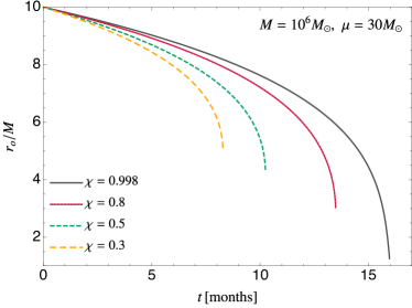
Figure 1: Evolution of the orbital radius under radiation reaction when including the influence of tidal heating (i.e., when the central object is a perfect absorber, ${\cal R}=0$) for $M=10^{6}M_{\odot}$, $\mu=30M_{\odot}$ and various spin values. The evolution starts at $r_{o}=10M$ and ends at the ISCO.

II.4 Circular equatorial orbits in Kerr and radiation reaction

Circular equatorial orbits in Kerr can be uniquely parametrized in terms of the energy $E$ and the angular momentum $L_{z}$ of the small orbiting body given by:

$$\frac{E}{\mu} = \frac{1-2v^{2}+\chi v^{3}}{\sqrt{1-3v^{2}+2\chi v^{3}}}\,,$$ (16)

$$\frac{L_{z}}{\mu} = \pm r_{o}v\frac{1-2\chi v^{3}+\chi^{2}v^{4}}{\sqrt{1-3v^{2}+2\chi v^{3}}}\,,$$ (17)

where $v\equiv\sqrt{M/r_{o}}$ and the plus and minus sign correspond to prograde and retrograde orbits, respectively.

Under the assumption that the evolution of the system under radiation reaction is adiabatic, i.e. the radiation reaction timescale is much longer than the orbital period, we evolve the system using the balance equation:

$$\dot{E}\equiv\dot{r}_{o}\frac{dE}{dr}=-\dot{E}_{\rm GW}\,,$$ (18)

where $\dot{E}_{\rm GW}$ is the total GW flux. The evolution of the orbital phase $\phi$ can then be computed using

$$\dot{\phi}=\Omega(t)\equiv\pm\frac{M^{1/2}}{r_{o}(t)^{3/2}+aM^{1/2}}\,.$$ (19)

An example of the evolution of the orbital radius under radiation reaction when including the influence of tidal heating (i.e. when ${\cal R}=0$) is shown in Fig. 1 for $M=10^{6}M_{\odot}$, $\mu=30M_{\odot}$, and various spin values. The evolution starts at $r_{o}=10M$ up to the ISCO, so that in the highly-spinning case the evolution lasts longer.

In the following we will be interested in computing the GW phase shift between an EMRI in a BH or ECO background. To do so we take into account the fact that the GW phase of the dominant mode is given by $\phi_{\rm GW}=2\phi$ and define the instantaneous dephasing as

$$\delta{\phi}(t)=\phi^{\rm BH}_{\rm GW}(t)-\phi^{\rm ECO}_{\rm GW}(t)\,,$$ (20)

where $\phi^{\rm BH}_{\rm GW}(t)$ and $\phi^{\rm ECO}_{\rm GW}(t)$ denote the instantaneous GW phase in the BH and ECO case, respectively, and we have chosen the initial conditions such that $\phi^{\rm BH}_{\rm GW}(t=0)=\phi^{\rm ECO}_{\rm GW}(t=0)$ at the initial orbital radius of the evolution.

In addition we also define the total dephasing accumulated up to a radius $r_{f}$ as

$$\Delta{\phi}=\phi^{\rm BH}_{\rm GW}(r_{o}=r_{f})-\phi^{\rm ECO}_{\rm GW}(r_{o}=r_{f})\,,$$ (21)

where $\phi^{\rm BH,ECO}_{\rm GW}(r_{o}=r_{f})$ is computed at the time where the orbital radius reaches $r_{f}$ and where again we set the orbital phase to be the same for both the BH and ECO case at the initial orbital radius.

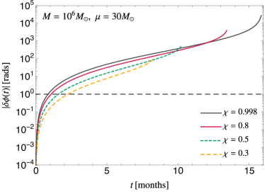
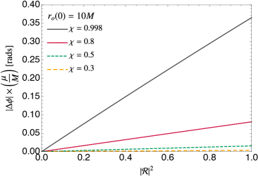
Figure 2: Left panel: dephasing due to absence of tidal heating in a perfectly-reflective ECO ($|{\cal R}|^{2}=1$) relative to the BH case (${\cal R}=0$). We consider a prototypical EMRI system and the evolution starts at $r_{o}=10M$ up to the ISCO for various values of the spin of the central object. Right panel: total dephasing accumulated from $r_{o}=10M$ up to the ISCO as a function of the reflectivity $|{\cal R}|^{2}$. Each line represents an interpolation of 20 equally spaced data points ranging from $|{\cal R}|^{2}=0$ up to $|{\cal R}|^{2}=1$. The dependence is linear for any value of the spin and of the other parameters.

II.5 Description of the code

We integrate the perturbation equations and compute fluxes and waveforms using the Gremlin code available in the Black Hole Perturbation Toolkit BHPToolkit . This code uses an accurate continued-fraction representation of the solution to Teukolsky equation Fujita:2009uz ; Fujita:2004rb . More specifically, the solutions $R^{\rm up,in}_{\ell m\omega}$ of the homogeneous Teukolsky equation are expanded as a series of hypergeometric functions; the coefficients of the series are determined by a three-term recurrence relation Sasaki:2003xr .

We used Gremlin to solve Teukolsky equation for all $m$ modes up to $\ell=\ell_{max}=20$ over a range of orbital radii. With the solutions for each $(\ell,m)$ mode at hand, the energy fluxes can be computed by summing over all modes using Eq. (10) and (11), respectively. Thus, the fluxes are computed as a function of the orbital radius; data are evenly spaced in the range from $r=20M$ to the ISCO, the latter depending on the value of the spin of the central object. At the ISCO, the fractional accuracy for the flux at infinity is $10^{-4}$ and for the flux at the horizon it is $10^{-8}$ Taracchini:2013wfa . Finally, fluxes are used to evolve the orbital trajectory of the small body adiabatically starting at $r_{o}=10M$, together with the corresponding GW signal.

The adiabatic inspiral is driven by the energy loss from the orbit via GWs at infinity and tidal heating. To compute the contribution of tidal heating we generated several sets of waveforms for different spin values. One set of waveforms is constructed where the inspiral is driven by both tidal heating and GW emission to infinity. The other family of waveforms is constructed by considering different values for $|{\cal R}|^{2}$. We use these waveforms to calculate the mismatch as explained below.

III Results

In the left panel of Fig. 2 we show the phase difference as a function of time for the case of a perfectly-reflective ECO ($|{\cal R}|^{2}=1$) and a BH with the same mass and spin. As a representative example, we use the same configurations as in Fig. 1. The orbit is again evolved from $r_{o}=10M$ up to the ISCO, so that in the highly-spinning case the evolution lasts longer and the total dephasing is larger.

The dashed horizontal line in the left panel of Fig. 2 marks the threshold $\delta\phi=1\,{\rm rad}$, which gives a very rough indication of the importance of tidal heating. As a rough but useful rule of thumb, if omission of tidal heating leads to dephasing $\delta\phi\approx 1\,{\rm rad}$ or greater as compared to a model that includes tidal heating, then its omission is likely to substantially impact a matched-filter search, leading to a significant loss of detected events Lindblom:2008cm . We emphasize that this rule of thumb must be validated with a more careful analysis; for example, correlations may allow for detection with incorrect models, albeit at the cost of systematic errors in fitted parameters. As expected, both the total and the instantaneous dephasing grow with the spin Hughes:2001jr . In the example of Fig. 2, for $\chi=0.3$, $\delta\phi\gtrsim 1\,{\rm rad}$ after slightly more than two months, whereas the same dephasing occurs after one month when $\chi\approx 0.9$. Overall, the total dephasing accumulated up to the ISCO is large, ranging from $10^{2}\,{\rm rad}$ to $10^{4}\,{\rm rad}$, depending on the spin.

In the right panel of Fig. 2 we show the dependence of the total dephasing with the reflectivity $|{\cal R}|^{2}$. The dependence is linear, $\Delta\phi\propto|{\cal R}|^{2}$, to an excellent accuracy. This is true also up to $|{\cal R}|^{2}\sim 1$, whereas the instantaneous dephasing $\delta\phi\propto|{\cal R}|^{2}$ only in the small-$|{\cal R}|^{2}$ or in the small-spin limit. The $\Delta\phi\propto|{\cal R}|^{2}$ scaling allows us to compute the total dephasing for a single value of ${\cal R}$ and re-scale the final result for different values of the reflectivity a posteriori. For example, the dephasing for $|{\cal R}|^{2}=1/2$ would be approximately half of what shown in the left panel of Fig. 2.

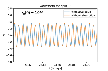
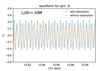
Figure 3: Comparison between waveforms computed with $|{\cal R}|^{2}=0$ (with absorption) and $|{\cal R}|^{2}=1$ (without absorption). We show the waveforms as function of time for $M=10^{6}M_{\odot}$, $\mu=30M_{\odot}$ and an orbit with initial radius $r_{o}(0)=10M$ and an initial phase $\phi(0)=0$. We show a number of cycles roughly $23$ days after the beginning of the orbit, for $\chi=0.7$ (top) and $\chi=0.9$ (bottom). For larger spins the effect of tidal heating (i.e., of nonzero reflectivity at the surface of the central object) is more pronounced leading to larger dephasing between the waveforms.

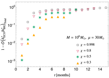
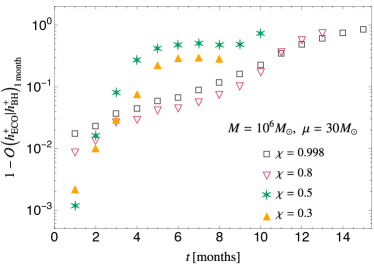
Figure 4: Left panel: mismatch ${\cal M}=1-{\cal O}$ as a function of observation time between the plus polarization for a waveform computed with $|{\cal R}|^{2}=1$ (ECO) and another computed with $|{\cal R}|^{2}=0$ (BH), maximized over time and phase shift. We consider the same systems as in Fig. 1. Right panel: mismatch over chunks of one month at different stages of the evolution.

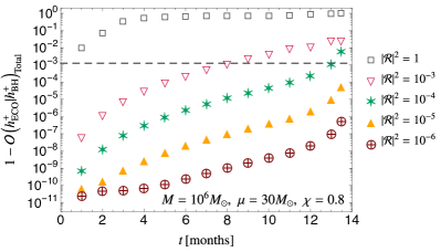
Figure 5: Same as left panel of Fig. 4 but also considering small $|{\cal R}|^{2}$ and for a central BH spin $\chi=0.8$. The dashed horizontal line marks the threshold $\mathcal{M}=1/(2\rho^{2})$, with $\rho=20$ being the fiducial SNR of the true signal.

Note that absorption – either total at the horizon or partial due to a partially reflecting ECO – also changes the mass and spin of the central object, in turn modifying the quasi-geodesic motion of the small orbiting body. This effect is always much smaller than the dissipative effect due to tidal heating. Even for a highly-spinning central object, this effect can account at most for a dephasing of $10^{-3}\,{\rm rad}$ Hughes_2019 , which is negligible compared to the effects shown in Fig. 2.

In Fig. 3 we show two representative examples (for spin $\chi=0.7$ and $\chi=0.9$ in the top and bottom panels, respectively) of the GW waveform emitted during the EMRI to leading order in the mass ratio. Also in this case the effect of heating grows significantly with the spin and becomes even appreciable by the naked eye when $\chi\gtrsim 0.9$.

Although the dephasing of the waveform is a useful measure to estimate the impact of tidal heating in the GW waveform, a better measure to assess whether the effect is sufficiently strong to be measurable in a GW detector with noise power spectral density (PSD) $S_{n}(f)$, is to compute the overlap $\mathcal{O}$ between two waveforms $h_{1}(t)$ and $h_{2}(t)$:

$$\mathcal{O}(h_{1}|h_{2})=\frac{\left\langle h_{1}|h_{2}\right\rangle}{\sqrt{\left\langle h_{1}|h_{1}\right\rangle\left\langle h_{2}|h_{2}\right\rangle}}\,,$$ (22)

where the noise-weighted inner product $\left\langle h_{1}|h_{2}\right\rangle$ is defined by

$$\left\langle h_{1}|h_{2}\right\rangle=4\Re\,\int_{0}^{\infty}\frac{\tilde{h}_{1}\tilde{h}^{*}_{2}}{S_{n}(f)}df\,.$$ (23)

Here the tilded quantities stand for the Fourier transform and the star for complex conjugation. Since the waveforms are defined up to an arbitrary time and phase shift, it is also necessary to maximize the overlap (22) over these quantities. In practice this can be done by computing Allen:2005fk

$$\mathcal{O}(h_{1}|h_{2})=\frac{4}{\sqrt{\left\langle h_{1}|h_{1}\right\rangle\left\langle h_{2}|h_{2}\right\rangle}}\max_{t_{0}}\left|\mathcal{F}^{-1}\left[\frac{\tilde{h}_{1}\tilde{h}^{*}_{2}}{S_{n}(f)}\right](t_{0})\right|\,,$$ (24)

where $\mathcal{F}^{-1}[g(f)](t)=\int_{-\infty}^{+\infty}g(f)e^{-2\pi ift}df$ represents the inverse Fourier transform. The overlap is defined such that $\mathcal{O}=1$ indicates a perfect agreement between the two waveforms. For the PSD we use the LISA curve of Ref. Cornish:2018dyw adding the contribution of the confusion noise from the unresolved Galactic binaries for a one year mission lifetime.

In Fig. 4 we show the mismatch $\mathcal{M}\equiv 1-{\cal O}$ for the plus polarization of the waveforms with $|{\cal R}|^{2}=1$ and $|{\cal R}|^{2}=0$, for the systems considered in Fig. 1. In the left plot of Fig. 4 we show of the mismatch as a function of observation time for orbits starting at $r_{o}(0)=10M$. For all the cases considered the mismatch $\mathcal{M}<0.02$ until the first month of observation, however it quickly increases as the small object approaches the ISCO, making the waveforms clearly distinguishable from one another. In the right plot of Fig. 4 we instead divide the waveforms in chunks of one month and compute the mismatch for that particular month of data. This allows us to assess how close are the waveforms at different stages of the evolution. As expected, the closer the object is from the ISCO the smaller the overlap. In particular for small spins the mismatch is $\mathcal{M}<0.1$ for most of the evolution. Finally, in Fig. 5 we show how the mismatch depends on the reflectivity for small values of $|{\cal R}|^{2}$ for the system with $\chi=0.8$. As expected, the mismatch decreases with $|{\cal R}|^{2}$. We find that for $|{\cal R}|^{2}\lesssim 10^{-4}$ the mismatch behaves roughly as ${\cal M}\propto|{\cal R}|^{4}$. Indeed, in the small dephasing limit, ${\cal O}\propto\cos\delta\phi$ Lindblom:2008cm and – owing to the $\delta\phi\propto|{\cal R}|^{2}$ dependence – the mismatch should scale as ${\cal M}\propto|{\cal R}|^{4}$, in agreement with our results.

IV Discussion

As a useful rule of thumb two waveforms are considered indistinguishable for parameter estimation purposes if $\mathcal{M}\lesssim 1/(2\rho^{2})$ Flanagan:1997kp ; Lindblom:2008cm , where $\rho$ is the SNR of the true signal. For an EMRI with an SNR $\rho\approx 20$ (resp., $\rho\approx 100$) one has $\mathcal{M}\lesssim 10^{-3}$ (resp., $\mathcal{M}\lesssim 5\times 10^{-5}$). As a reference, in Fig. 5 we mark the threshold $\mathcal{M}=10^{-3}$ with a dashed horizontal line. It is clear from Figs. 4 and 5 that this level of mismatch is quickly exceeded in an EMRI due to absence/presence of tidal heating for a perfecly-reflecting ECO (i.e., when $|{\cal R}|=1$), even for small spins. This implies that the reflectivity $|{\cal R}|^{2}$ can be constrained down to very small values. For example considering a supermassive object with $\chi\gtrsim 0.8$ and a signal with $\rho=20$, from the results in Fig. 5 we can estimate a very stringent bound on the reflectivity

$$|{\cal R}|^{2}\lesssim 5\times 10^{-5}\,.$$ (25)

A more conservative bound would be obtained by requiring that the dephasing be smaller than $1\,{\rm rad}$. Owing to the $\delta\phi\propto|{\cal R}|^{2}$ dependence and considering also $\chi\gtrsim 0.8$, we find the slightly weaker constraint $|{\cal R}|^{2}\lesssim 10^{-4}$. Thus, an EMRI detection is sensitive to an effective reflectivity of the central supermassive object as small as $\sim{\cal O}(0.01\%)$ (as a reference, we remind that in the BH case the reflectivity is zero and that for a neutron star it is practically unity, even when accounting for dissipation 1971ApJ…165..165E ).

The above results confirm previous findings that advocated for the importance of tidal heating in standard EMRI waveforms Hughes:2001jr ; Taracchini:2013wfa : heating needs to be modelled accurately in order not to introduce a large dephasing and systematic errors. In addition, we showed that the inclusion/absence of tidal heating can be used as a strong, model independent, discriminator for the presence of a horizon in the central supermassive object.

Compared to other types of observations, this is a very stringent bound. For instance, in order to achieve a bound of the order of Eq. (25) at $2\sigma$ confidence level from a negative echo search in the ringdown of a comparable-mass binary merger, a SNR of ${\cal O}(10^{3})$ in the ringdown would be needed Maggio:2019zyv . Reaching $3\sigma$ confidence level for the same bound would require a SNR of ${\cal O}(10^{4})$ in the ringdown, which is well beyond what is expected with LISA, even for the loudest mergers Audley:2017drz (although such loud signals might be possible with future extensions Baibhav:2019rsa ).

Our analysis relies only on the modification of the fluxes at the leading order in the mass ratio, i.e., we included only the leading-order dissipative part of the self-force Poisson:2003nc ; Barack:2009ux , neglecting conservative contributions and higher-order terms. While conservative contributions and high-order terms are crucially important for parameter estimation, their impact is not likely to be confused for that of tidal heating, since tidal heating effects are typically much stronger, at least for realistic values of the spin and when ${\cal R}$ is not negligibly small. Thus, we expect that reliable constraints can be obtained by modelling (partial) absence of tidal heating in state-of-the-art waveform approximants to the leading order, along with – and independently of – other self-force corrections.

We considered here the simplest trajectory, namely a circular equatorial orbit, but we expect that our results would remain qualitatively the same for more generic trajectories. Eccentric orbits can probe regions closer to the central object than in the circular case, so the effect of tidal heating may be expected to be even larger in that case. On the other hand, the relative effect of tidal heating on the orbit tends to be smaller for highly non-equatorial orbits Hughes:2001jr .

Another natural extension of our work concerns the role of resonances due to the excitation of low-frequency quasinormal modes which are ubiquitous for ECOs Pani:2010em ; Macedo:2013jja ; Cardoso:2019rvt . These resonances are very narrow and have been shown to produce a negligible effect in the nonspinning case Cardoso:2019nis . It would be interesting to include them in a spinning model and to investigate the possible existence of floating orbits, namely the possibility that for certain circular orbits the (negative) flux emitted to infinity can be compensated by a (positive, due to superradiance) flux at the horizon, in the case the latter is resonantly enhanced Cardoso:2011xi . If this condition occurs the orbits can be metastable and introduce a large dephasing. However, preliminary analysis shows that the effect of tidal heating discussed here should nonetheless be dominant.

Finally, we made the conservative assumption that the external geometry of the central object can be described by the Kerr metric. ECOs might display several multipolar deviations from Kerr, whose amplitude – in the ultracompact regime – is bounded by regularity arguments Raposo:2018xkf ; Barcelo:2019aif . These deviations affect also the conservative part of the EMRI dynamics to the leading order in the mass ratio and would introduce a further diagnostic for the presence of horizons, similarly to the case of “bumpy” BHs Collins:2004ex ; Vigeland:2009pr ; Moore:2017lxy .

Appendix A Energy fluxes: ECOs vs BHs

In this appendix we study the differences in the energy fluxes between a BH and an ECO.

A.1 Energy flux at infinity

Here we show that the energy flux at infinity due to a point particle in circular motion around a Kerr-like object is independent (within numerical accuracy) of the boundary conditions at the surface of the object (modulo narrow resonances). As a by-product, the flux is the same for a BH and for an ECO. Our study extends that done in Ref. Cardoso:2019nis , in which low-frequency perturbations of nonspinning objects were considered. Instead, we consider the case in which the spin of the object and the frequency of the perturbations are arbitrary.

Our starting point is Teukolsky’s equation (3). It is convenient to make a change of variables by introducing the Detweiler’s function 1977RSPSA.352..381D ; Maggio:2018ivz

$$\Psi=\Delta^{-1}\sqrt{r^{2}+a^{2}}\left[\alpha\ R_{lm\omega}+\beta\Delta^{-1}\frac{dR_{lm\omega}}{dr}\right]\,,$$ (26)

where $\alpha$ and $\beta$ are certain radial functions 1977RSPSA.352..381D ; Maggio:2018ivz . By introducing the tortoise coordinate $x$ as in Eq. (6), Teukolsky’s master equation becomes

$$\frac{d^{2}\Psi}{dx^{2}}-V(r,\omega)\Psi=S\,.$$ (27)

where $S$ is a source term and the final potential $V$ is defined, e.g., in Ref. Maggio:2018ivz . The asymptotic behavior of the potential is $V\to-\omega^{2}$ as $x\to\infty$ and $V\to-k^{2}$ as $x\to-\infty$. The functions $\alpha$ and $\beta$ can be chosen such that the resulting potential $V$ is purely real 1977RSPSA.352..381D ; Maggio:2018ivz . Although the choice of $\alpha$ and $\beta$ is not unique, ${\Psi}$ evaluated at the asymptotic infinities ($x\to\pm\infty$) remains unchanged up to a phase. Therefore, the energy and angular momentum fluxes are not affected MTB .

As discussed in the main text, the solution to Eq. (27) can be found in term of the Green’s function as

$$\Psi=\frac{\Psi_{+}}{W}\int_{-\infty}^{x}dx\,\Psi_{-}S+\frac{\Psi_{-}}{W}\int^{+\infty}_{x}dx\,\Psi_{+}S\,,$$ (28)

where $\Psi_{\pm}$ are two solutions of the homogeneous equation which satisfy the correct boundary conditions at infinity (for the plus sign) and near the object (for the minus sign), whereas $W=\frac{d\Psi_{+}}{dx}\Psi_{-}-\Psi_{+}\frac{d\Psi_{-}}{dx}$ is their Wronskian. Regardless of the nature of the central object, the boundary condition at infinity reads

$$\Psi\propto\Psi_{+}\sim e^{i\omega x}\,.$$ (29)

Given an object with reflectivity ${\cal R}$, the boundary condition near its surface ($x=x_{0}\to-\infty$) is Mark:2017dnq

$$\Psi\propto\Psi_{-}\sim e^{-ik(x-x_{0})}+{\cal R}e^{ik(x-x_{0})}\,.$$ (30)

As discussed in the main text the flux at infinity can be computed as $\dot{E}_{\infty}\propto|\Psi(x\to\infty)|^{2}$, where

$$\Psi(x\to\infty)=\frac{e^{i\omega x}}{W}\int_{-\infty}^{+\infty}dx\Psi_{-}S\,.$$ (31)

For a point particle in circular equatorial motion, the source term can be schematically written as

$$S=A(\omega)\delta(x-x_{o})+B(\omega)\delta^{\prime}(x-x_{o})\,,$$ (32)

where $x_{o}=x(r_{o})$ is the orbital radius in tortoise coordinates. Then, standard treatment Martel:2005ir leads to the following solution

$$\Psi(x\to\infty)=\left.e^{i\omega x}\frac{\hat{A}(\omega)\Psi_{-}(r_{o})+\hat{B}(\omega){\Psi_{-}^{\prime}}(r_{o})}{W}\right|_{\omega=m\Omega}\,,$$ (33)

where $\hat{A}$ and $\hat{B}$ are two functions of the frequency related to $A$ and $B$ in Eq. (32).

Finally, one can solve numerically the homogeneous equation with boundary conditions given by Eqs. (29) and (30) in order to evaluate $\Psi_{-}$ and the Wronskian, and using the explicit form of the source term for circular orbits. One can verify numerically that $\Psi(x\to\infty)$ appearing in Eq. (33) does not depend on the value of ${\cal R}$ in Eq. (30), at least within the numerical accuracy of our code. In particular, the energy flux at infinity is the same regardless the value of ${\cal R}$, including the BH case (${\cal R}=0$). This argument is valid far from possible resonances in the flux. These resonances correspond to the poles of the Wronskian $W$, which occur near the real axis in the complex plane. Since the fundamental quasinormal modes of an ECO have very small imaginary part Pani:2009ss ; Maggio:2017ivp ; Maggio:2018ivz , these resonances are extremely narrow Pani:2010em ; Macedo:2013jja and their contribution to the dynamics is negligible Cardoso:2019nis .

An alternative way to understand this result is the following. A point particle in circular motion emits monochromatic radiation. Part of the latter goes directly to infinity, contributing to $\dot{E}_{\infty}$ regardless of the boundary conditions near the central object. Another fraction of the radiation is either reflected by the potential barrier produced by the gravitational field of the object (both in the BH and in the ECO case) or partially reflected by the surface of the object (only in the ECO case). In both cases this radiation is reflected back at the same frequency and can therefore be efficiently re-absorbed by the orbting particle, which therefore does not lose the corresponding energy. This occurs as long as $T_{\rm arr}\lesssim T_{\rm RR}$ [cf. Eqs. (13) and (14)], which is typically the case, as we showed in the main text.

A.2 Energy flux at the ECO surface

Here we show that the energy flux at the ECO surface can be expressed as a fraction of the energy flux at the horizon of a Kerr BH with the same mass and spin. In the ECO case, the boundary condition in Eq. (30) represents the sum of an ingoing wave and of an outgoing wave with relative amplitude ${\cal R}$.

Assuming $|x_{0}|\gg M$, we can evaluate the flux as $x\to-\infty$. For the ingoing wave, this flux will be proportional to (the square of the absolute value of)

$$\Psi_{\rm absorbed}(x\to-\infty)=\frac{1}{W}\int_{-\infty}^{+\infty}dx\,\Psi_{+}S\,,$$ (34)

where $\Psi_{+}$ is the solution which is regular at infinity, and it is the same for both the BH and the ECO cases. Notice that $\dot{E}_{H}\propto|\Psi_{\rm absorbed}(x\to-\infty)|^{2}$ is the energy flux at the horizon in the BH case. In the ECO case, there is an extra contribution due to the outgoing wave in Eq. (30). The flux in this case will be proportional to (the square of the absolute value of)

$$\Psi_{\rm reflected}(x\to-\infty)=\frac{{\cal R}}{W}\int_{-\infty}^{+\infty}dx\,\Psi_{+}S\,.$$ (35)

Notice that this contribution has the opposite sign in the flux, since it accounts for energy that crosses the object’s surface in the opposite direction. Since $\Psi_{+}$ is independent of ${\cal R}$, the integral in Eqs. (34) and (35) is the same, so the ratio of the absorbed to reflected fluxes is

$$\frac{\dot{E}_{\rm absorbed}}{\dot{E}_{\rm reflected}}=|{\cal R}|^{2}\,.$$ (36)

Finally, since the two contribution have opposite sign, we obtain Eq. (12) in the main text.

References

- (1) V. Cardoso and P. Pani, “Testing the nature of dark compact objects: a status report,” Living Rev. Rel. 22 no. 1, (2019) 4, arXiv:1904.05363 [gr-qc].
- (2) N. Oshita, Q. Wang, and N. Afshordi, “On Reflectivity of Quantum Black Hole Horizons,” arXiv:1905.00464 [hep-th].
- (3) R. Brito, V. Cardoso, and P. Pani, “Superradiance,” Lect. Notes Phys. 906 (2015) pp.1–237, arXiv:1501.06570 [gr-qc].
- (4) K. S. Thorne, R. Price, and D. Macdonald, Black holes: the membrane paradigm. Yale University Press, 1986.
- (5) T. Damour, “Pulsating relativistic stars,” in Proceedings of the Second Marcel Grossmann Meeting ofGeneral Relativity, edited by R. Ruffini, North Holland, Amsterdam, 1982 pp 587-608. 1982.
- (6) E. Poisson, “Tidal interaction of black holes and Newtonian viscous bodies,” Phys. Rev. D80 (2009) 064029, arXiv:0907.0874 [gr-qc].
- (7) V. Cardoso and P. Pani, “Tidal acceleration of black holes and superradiance,” Class. Quant. Grav. 30 (2013) 045011, arXiv:1205.3184 [gr-qc].
- (8) J. B. Hartle, “Tidal Friction in Slowly Rotating Black Holes,” Phys. Rev. D8 (1973) 1010–1024.
- (9) S. A. Hughes, “Evolution of circular, nonequatorial orbits of kerr black holes due to gravitational-wave emission. ii. inspiral trajectories and gravitational waveforms,” Phys. Rev. D 64 (Aug, 2001) 064004. https://link.aps.org/doi/10.1103/PhysRevD.64.064004.
- (10) E. Poisson and C. Will, Gravity: Newtonian, Post-Newtonian, Relativistic. Cambridge University Press, Cambridge, UK, 1953.
- (11) S. A. Hughes, “Evolution of circular, nonequatorial orbits of Kerr black holes due to gravitational wave emission. II. Inspiral trajectories and gravitational wave forms,” Phys. Rev. D64 (2001) 064004, arXiv:gr-qc/0104041 [gr-qc]. [Erratum: Phys. Rev.D88,no.10,109902(2013)].
- (12) S. Bernuzzi, A. Nagar, and A. Zenginoglu, “Horizon-absorption effects in coalescing black-hole binaries: An effective-one-body study of the non-spinning case,” Phys. Rev. D86 (2012) 104038, arXiv:1207.0769 [gr-qc].
- (13) A. Taracchini, A. Buonanno, S. A. Hughes, and G. Khanna, “Modeling the horizon-absorbed gravitational flux for equatorial-circular orbits in Kerr spacetime,” Phys. Rev. D88 (2013) 044001, arXiv:1305.2184 [gr-qc]. [Erratum: Phys. Rev.D88,no.10,109903(2013)].
- (14) E. Harms, S. Bernuzzi, A. Nagar, and A. Zenginoglu, “A new gravitational wave generation algorithm for particle perturbations of the Kerr spacetime,” Class. Quant. Grav. 31 no. 24, (2014) 245004, arXiv:1406.5983 [gr-qc].
- (15) S. Datta and S. Bose, “Probing the nature of central objects in extreme-mass-ratio inspirals with gravitational waves,” arXiv:1902.01723 [gr-qc].
- (16) H. Audley, S. Babak, J. Baker, E. Barausse, P. Bender, E. Berti, P. Binetruy, M. Born, D. Bortoluzzi, J. Camp, C. Caprini, V. Cardoso, M. Colpi, J. Conklin, N. Cornish, C. Cutler, et al., “Laser Interferometer Space Antenna,” ArXiv e-prints (Feb., 2017) , arXiv:1702.00786 [astro-ph.IM].
- (17) V. Baibhav et al., “Probing the Nature of Black Holes: Deep in the mHz Gravitational-Wave Sky,” arXiv:1908.11390 [astro-ph.HE].
- (18) A. Maselli, P. Pani, V. Cardoso, T. Abdelsalhin, L. Gualtieri, and V. Ferrari, “Probing Planckian corrections at the horizon scale with LISA binaries,” Phys. Rev. Lett. 120 no. 8, (2018) 081101, arXiv:1703.10612 [gr-qc].
- (19) F. D. Ryan, “Gravitational waves from the inspiral of a compact object into a massive, axisymmetric body with arbitrary multipole moments,” Phys. Rev. D52 (1995) 5707–5718.
- (20) L. Barack and C. Cutler, “Using LISA EMRI sources to test off-Kerr deviations in the geometry of massive black holes,” Phys. Rev. D75 (2007) 042003, arXiv:gr-qc/0612029 [gr-qc].
- (21) S. Babak, J. Gair, A. Sesana, E. Barausse, C. F. Sopuerta, C. P. L. Berry, E. Berti, P. Amaro-Seoane, A. Petiteau, and A. Klein, “Science with the space-based interferometer LISA. V: Extreme mass-ratio inspirals,” Phys. Rev. D95 no. 10, (2017) 103012, arXiv:1703.09722 [gr-qc].
- (22) P. Pani and A. Maselli, “Love in Extrema Ratio,” arXiv:1905.03947 [gr-qc].
- (23) G. Raposo, P. Pani, and R. Emparan, “Exotic compact objects with soft hair,” Phys. Rev. D99 no. 10, (2019) 104050, arXiv:1812.07615 [gr-qc].
- (24) C. Barcelo, R. Carballo-Rubio, and S. Liberati, “Generalized no-hair theorems without horizons,” arXiv:1901.06388 [gr-qc].
- (25) P. Pani, E. Berti, V. Cardoso, Y. Chen, and R. Norte, “Gravitational wave signatures of the absence of an event horizon. I. Nonradial oscillations of a thin-shell gravastar,” Phys. Rev. D80 (2009) 124047, arXiv:0909.0287 [gr-qc].
- (26) E. Maggio, P. Pani, and V. Ferrari, “Exotic Compact Objects and How to Quench their Ergoregion Instability,” Phys. Rev. D96 no. 10, (2017) 104047, arXiv:1703.03696 [gr-qc].
- (27) E. Maggio, V. Cardoso, S. R. Dolan, and P. Pani, “Ergoregion instability of exotic compact objects: electromagnetic and gravitational perturbations and the role of absorption,” Phys. Rev. D99 no. 6, (2019) 064007, arXiv:1807.08840 [gr-qc].
- (28) P. Pani, E. Berti, V. Cardoso, Y. Chen, and R. Norte, “Gravitational-wave signatures of the absence of an event horizon. II. Extreme mass ratio inspirals in the spacetime of a thin-shell gravastar,” Phys. Rev. D81 (2010) 084011, arXiv:1001.3031 [gr-qc].
- (29) C. F. B. Macedo, P. Pani, V. Cardoso, and L. C. B. Crispino, “Astrophysical signatures of boson stars: quasinormal modes and inspiral resonances,” Phys. Rev. D88 no. 6, (2013) 064046, arXiv:1307.4812 [gr-qc].
- (30) V. Cardoso, A. del Rio, and M. Kimura, “Distinguishing black holes from horizonless objects through the excitation of resonances during inspiral,” arXiv:1907.01561 [gr-qc].
- (31) J. Abedi, H. Dykaar, and N. Afshordi, “Echoes from the Abyss: Tentative evidence for Planck-scale structure at black hole horizons,” Phys. Rev. D96 no. 8, (2017) 082004, arXiv:1612.00266 [gr-qc].
- (32) Q. Wang and N. Afshordi, “Black hole echology: The observer’s manual,” Phys. Rev. D97 no. 12, (2018) 124044, arXiv:1803.02845 [gr-qc].
- (33) E. Barausse, R. Brito, V. Cardoso, I. Dvorkin, and P. Pani, “The stochastic gravitational-wave background in the absence of horizons,” Class. Quant. Grav. 35 no. 20, (2018) 20LT01, arXiv:1805.08229 [gr-qc].
- (34) P. Pani, “I-Love-Q relations for gravastars and the approach to the black-hole limit,” Phys. Rev. D92 no. 12, (2015) 124030, arXiv:1506.06050 [gr-qc].
- (35) N. Uchikata and S. Yoshida, “Slowly rotating thin shell gravastars,” Class. Quant. Grav. 33 no. 2, (2016) 025005, arXiv:1506.06485 [gr-qc].
- (36) N. Uchikata, S. Yoshida, and P. Pani, “Tidal deformability and I-Love-Q relations for gravastars with polytropic thin shells,” Phys. Rev. D94 no. 6, (2016) 064015, arXiv:1607.03593 [gr-qc].
- (37) K. Yagi and N. Yunes, “I-Love-Q anisotropically: Universal relations for compact stars with scalar pressure anisotropy,” Phys. Rev. D91 no. 12, (2015) 123008, arXiv:1503.02726 [gr-qc].
- (38) K. Yagi and N. Yunes, “Relating follicly-challenged compact stars to bald black holes: A link between two no-hair properties,” Phys. Rev. D91 no. 10, (2015) 103003, arXiv:1502.04131 [gr-qc].
- (39) C. Posada, “Slowly rotating supercompact Schwarzschild stars,” Mon. Not. Roy. Astron. Soc. 468 no. 2, (2017) 2128–2139, arXiv:1612.05290 [gr-qc].
- (40) S. Drasco and S. A. Hughes, “Gravitational wave snapshots of generic extreme mass ratio inspirals,” Phys. Rev. D73 no. 2, (2006) 024027, arXiv:gr-qc/0509101 [gr-qc]. [Erratum: Phys. Rev.D90,no.10,109905(2014)].
- (41) S. A. Hughes, “The Evolution of circular, nonequatorial orbits of Kerr black holes due to gravitational wave emission,” Phys. Rev. D61 no. 8, (2000) 084004, arXiv:gr-qc/9910091 [gr-qc]. [Erratum: Phys. Rev.D90,no.10,109904(2014)].
- (42) S. O’Sullivan and S. A. Hughes, “Strong-field tidal distortions of rotating black holes: Formalism and results for circular, equatorial orbits,” Phys. Rev. D90 no. 12, (2014) 124039, arXiv:1407.6983 [gr-qc]. [Erratum: Phys. Rev.D91,no.10,109901(2015)].
- (43) Z. Mark, A. Zimmerman, S. M. Du, and Y. Chen, “A recipe for echoes from exotic compact objects,” Phys. Rev. D96 no. 8, (2017) 084002, arXiv:1706.06155 [gr-qc].
- (44) V. Cardoso, L. C. B. Crispino, C. F. B. Macedo, H. Okawa, and P. Pani, “Light rings as observational evidence for event horizons: long-lived modes, ergoregions and nonlinear instabilities of ultracompact objects,” Phys. Rev. D90 no. 4, (2014) 044069, arXiv:1406.5510 [gr-qc].
- (45) V. Cardoso, E. Franzin, and P. Pani, “Is the gravitational-wave ringdown a probe of the event horizon?,” Phys. Rev. Lett. 116 no. 17, (2016) 171101, arXiv:1602.07309 [gr-qc].
- (46) V. Cardoso, S. Hopper, C. F. B. Macedo, C. Palenzuela, and P. Pani, “Gravitational-wave signatures of exotic compact objects and of quantum corrections at the horizon scale,” Phys. Rev. D94 no. 8, (2016) 084031, arXiv:1608.08637 [gr-qc].
- (47) “Black Hole Perturbation Toolkit.” (bhptoolkit.org).
- (48) R. Fujita and H. Tagoshi, “New Numerical Methods to Evaluate Homogeneous Solutions of the Teukolsky Equation II. Solutions of the Continued Fraction Equation,” Prog. Theor. Phys. 113 (2005) 1165–1182, arXiv:0904.3818 [gr-qc].
- (49) R. Fujita and H. Tagoshi, “New numerical methods to evaluate homogeneous solutions of the Teukolsky equation,” Prog. Theor. Phys. 112 (2004) 415–450, arXiv:gr-qc/0410018 [gr-qc].
- (50) M. Sasaki and H. Tagoshi, “Analytic black hole perturbation approach to gravitational radiation,” Living Rev. Rel. 6 (2003) 6, arXiv:gr-qc/0306120 [gr-qc].
- (51) L. Lindblom, B. J. Owen, and D. A. Brown, “Model Waveform Accuracy Standards for Gravitational Wave Data Analysis,” Phys. Rev. D78 (2008) 124020, arXiv:0809.3844 [gr-qc].
- (52) S. A. Hughes, “Bound orbits of a slowly evolving black hole,” Physical Review D 100 no. 6, (Sep, 2019) . http://dx.doi.org/10.1103/PhysRevD.100.064001.
- (53) B. Allen, W. G. Anderson, P. R. Brady, D. A. Brown, and J. D. E. Creighton, “FINDCHIRP: An Algorithm for detection of gravitational waves from inspiraling compact binaries,” Phys. Rev. D85 (2012) 122006, arXiv:gr-qc/0509116 [gr-qc].
- (54) T. Robson, N. J. Cornish, and C. Liug, “The construction and use of LISA sensitivity curves,” Class. Quant. Grav. 36 no. 10, (2019) 105011, arXiv:1803.01944 [astro-ph.HE].
- (55) E. E. Flanagan and S. A. Hughes, “Measuring gravitational waves from binary black hole coalescences: 2. The Waves’ information and its extraction, with and without templates,” Phys. Rev. D57 (1998) 4566–4587, arXiv:gr-qc/9710129 [gr-qc].
- (56) F. P. Esposito, “Absorption of Gravitational Energy by a Viscous Compressible Fluid,” Astrophys. J. 165 (Apr., 1971) 165.
- (57) E. Maggio, A. Testa, S. Bhagwat, and P. Pani, “Analytical model for gravitational-wave echoes from spinning remnants,” Phys. Rev. D100 no. 6, (2019) 064056, arXiv:1907.03091 [gr-qc].
- (58) E. Poisson, “The Motion of point particles in curved space-time,” Living Rev. Rel. 7 (2004) 6, arXiv:gr-qc/0306052 [gr-qc].
- (59) L. Barack, “Gravitational self force in extreme mass-ratio inspirals,” Class. Quant. Grav. 26 (2009) 213001, arXiv:0908.1664 [gr-qc].
- (60) V. Cardoso, S. Chakrabarti, P. Pani, E. Berti, and L. Gualtieri, “Floating and sinking: The Imprint of massive scalars around rotating black holes,” Phys. Rev. Lett. 107 (2011) 241101, arXiv:1109.6021 [gr-qc].
- (61) N. A. Collins and S. A. Hughes, “Towards a formalism for mapping the space-times of massive compact objects: Bumpy black holes and their orbits,” Phys. Rev. D69 (2004) 124022, arXiv:gr-qc/0402063 [gr-qc].
- (62) S. J. Vigeland and S. A. Hughes, “Spacetime and orbits of bumpy black holes,” Phys. Rev. D81 (2010) 024030, arXiv:0911.1756 [gr-qc].
- (63) C. J. Moore, A. J. K. Chua, and J. R. Gair, “Gravitational waves from extreme mass ratio inspirals around bumpy black holes,” Class. Quant. Grav. 34 no. 19, (2017) 195009, arXiv:1707.00712 [gr-qc].
- (64) S. Detweiler, “On resonant oscillations of a rapidly rotating black hole,” Proceedings of the Royal Society of London Series A 352 (July, 1977) 381–395.
- (65) S. Chandrasekhar, The Mathematical Theory of Black Holes. Oxford University Press, New York, 1983.
- (66) K. Martel and E. Poisson, “Gravitational perturbations of the Schwarzschild spacetime: A Practical covariant and gauge-invariant formalism,” Phys. Rev. D71 (2005) 104003, arXiv:gr-qc/0502028 [gr-qc].