Anomalous caustics and Veselago focusing in 8-Pmmn borophene p-n junctions with arbitrary junction directions

Abstract

Negative refraction usually demands complex structure engineering while it is very natural for massless Dirac fermions (MDFs) across the p-n junction, this leads to Dirac electron optics. The emergent Dirac materials may exhibit hitherto unidentified phenomenon due to their nontrivial band structures in contrast to the isotropic MDFs in graphene. Here, as a specific example, we explore the negative refraction induced caustics and Veselago focusing of tilted MDFs across 8-Pmmn borophene p-n junctions. To this aim, we develop a technique to effectively construct the electronic Green’s function in p-n junctions with arbitrary junction directions. Based on analytical discussions and numerical calculations, we demonstrate the strong dependence of interference pattern on the junction direction. As the junction direction perpendicular to the tilt direction, Veselago focusing or normal caustics (similar to that in graphene) appears resting on the doping configuration of the p-n junctions, otherwise anomalous caustics (different from that in graphene) occurs which is manipulated by the junction direction and the doping configuration. Finally, the developed Green’s function technique is generally promising to uncover the unique transport of emergent MDFs, and the discovered anomalous caustics makes tilted MDFs potential applications in Dirac electron optics.

I Introduction

Negative refraction is one unusual class of wave propagationPendry (2000), which leads to novel interference and hold great potential in new applicationsSmith et al. (2004). But its realization usually demands complex structure engineering with stringent parameter conditionsChen et al. (2016a). Graphene as the first two-dimensional material, hosts the relativistic massless Dirac fermions (MDFs) and possesses a lot of exotic physics and possible applications Castro Neto et al. (2009). Especially, the two-dimensional nature of graphene is beneficial to the fabrication of the planar p-n junction (PNJ), which is the basic component of many electronic devicesLow (2012); Frisenda et al. (2018). The propagation of MDFs across graphene PNJ has a close analogy to optical negative refraction at the surface of metamaterials but exhibits negative refraction in a more simple and tunable mannerCheianov et al. (2007). Recently, negative refraction in the graphene PNJ has been verified experimentallyLee et al. (2015); Chen et al. (2016b). As a result, there is wide interest to study the negative refraction induced interference of MDFs in the PNJ structureGarcia-Pomar et al. (2008); Moghaddam and Zareyan (2010); Silveirinha and Engheta (2013); Zhao et al. (2013); Milovanovic et al. (2015); Bøggild et al. (2017); Zhang et al. (2017a); Hills et al. (2017); Zhang et al. (2018); Betancur-Ocampo (2018); Prabhakar et al. (2019); Brun et al. (2019).

The great success of graphene attracts people to search for new two-dimensional materials in which quasiparticles can be described as MDFs Wehling et al. (2014); Wang et al. (2015), i.e., Dirac materials. Dirac materials emerge quickly and usually host very novel MDFs, in which new physics and application potential are expectedWehling et al. (2014); Wang et al. (2015); Xu et al. (2018). The Dirac fermions can be classified finely into four categoriesMilićević et al. (2019), i.e., type-I, type-I tilted, type-III (critical tilt), and type-II ones. These four categories of Dirac fermions are expected to exhibit distinct physical properties due to different geometries of their Fermi surface. To our knowledge, type-I tilted Dirac fermions has been predicted to appear in very rare systems including quinoid-type graphene and -(BEDT-TTF)₂I₃Goerbig et al. (2008), hydrogenated grapheneLu et al. (2016a), and 8-Pmmn boropheneZhou et al. (2014); Lopez-Bezanilla and Littlewood (2016); Zabolotskiy and Lozovik (2016); Nakhaee et al. (2018). In such Dirac materials, 8-Pmmn borophene as elemental monolayer material exhibits high mobility and anisotropic transportCheng et al. (2017), which has potential applications in electronics and electron optics. The well-established continuum model of 8-Pmmn borophene make it be very suitable to the model study. This anisotropy and tilt of type-I Dirac fermions brings about unique features to various physical properties of 8-Pmmn borophene, including plasmon Sadhukhan and Agarwal (2017); Jalali-Mola and Jafari (2018), the optical conductivity Verma et al. (2017), Weiss oscillations Islam and Jayannavar (2017), oblique Klein tunnelingZhang and Yang (2018), metal-insulator transition induced by strong electromagnetic radiationChampo and Naumis (2019), and RKKY interactionPaul et al. (2019); Zhang et al. (2019). Thus, it is expected that the anisotropy and tilt will strongly affect the negative refraction of MDFs cross 8-Pmmn borophene PNJ.

In this study, we investigate the negative refraction induced interference in 8-Pmmn borophene PNJs. Following the seminal study in grapheneCheianov et al. (2007), we focus on two typical interference pattern, i.e, caustics and Veselago focusing. Due to the anisotropy and tilt of MDFs in 8-Pmmn borophene, the interference pattern has inevitable dependence on the junction direction. Hence, we develop a construction technique of the electronic Green’s function (GF), which is applicable to the PNJ with an arbitrary junction direction. We find: (I) Veselago focusing or normal caustics appears resting on the doping configuration of the PNJ when its junction direction is perpendicular to the tilt direction of MDFs. (II) To the other junction, anomalous caustics unique to anisotropic and tilted MDFs occurs, and its pattern strongly depends on the junction direction and the doping configuration of the PNJ. We expect that the developed GF technique is used to study the other transport properties of continuing emergent MDFs, and the discovered anomalous caustics can be observed in near future pointing out the potential application of novel MDFs (in 8-Pmmn borophene or other Dirac materials) in Dirac electron optics.

The rest of this paper is organized as follows. In Sec. II, we introduce the model structures and Hamiltonian of the 8-Pmmn borophene PNJ, and present the detailed construction technique of the electronic GF. In Sec. III, according to the junction direction of PNJs, we demonstrate Veselago focusing and anomalous caustics by combing numerical calculations and analytical derivation. Finally, we summarize this study in Sec. IV.

II Theoretical formalism

II.1 Model and Hamiltonian

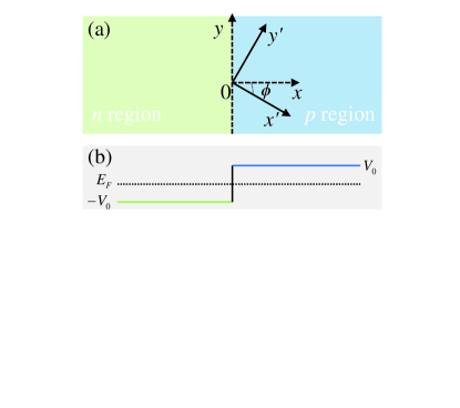
Figure 1: (a) Schematic p-n junction with the left n region and the right p region. Two Cartesian coordinate systems $x-y$ and $x^{\prime}-y^{\prime}$ are introduced, and $x-y$ has one rotation relative to the $x^{\prime}-y^{\prime}$ with the angle $\phi$. The normal (tangential) direction of the junction interface defines the $x$ ($y$) axis of the coordinate system $x-y$ while the coordinate system $x^{\prime}-y^{\prime}$ is used to express the intrinsic Hamiltonian. So $\phi$ is used to denote the junction direction. (b) The energy position $-V_{0}$ ($V_{0}$) for the Dirac point of the n (p) region relative to the aligned Fermi energy $E_{F}$.

We introduce the Cartesian coordinate system $x^{\prime}-y^{\prime}$ accompanying the intrinsic Hamiltonian $\hat{H}_{0}$ of 8-Pmmn borophene. In 8-Pmmn borophene, $\hat{H}_{0}$ describes the anisotropic and tilted MDFs, and has the valley dependence. However, we focus the new physics induced by the anisotropy and tilt, so the valley dependence of $\hat{H}_{0}$ is neglected in our model study. Around the Dirac point, $\hat{H}_{0}$ has the form Zabolotskiy and Lozovik (2016); Sadhukhan and Agarwal (2017); Islam and Jayannavar (2017)

$$\hat{H}_{0}=v_{1}\sigma_{1}\hat{p}_{x^{\prime}}+v_{2}\sigma_{2}\hat{p}_{y^{\prime}}+v_{t}\sigma_{0}\hat{p}_{y^{\prime}},$$ (1)

where $\hat{p}_{x^{\prime},y^{\prime}}$ are the momentum operators, $\sigma_{1,2}$ and $\sigma_{0}$ are Pauli matrices and $2\times 2$ identity matrix, respectively. The anisotropic velocities are $v_{1}=0.86v_{F}$, $v_{2}=0.69v_{F}$, and $v_{t}=0.32v_{F}$ with $v_{F}=10^{6}$ m/s. Throughout this paper, we set $\hbar=v_{F}\equiv 1$ to favor our dimensionless derivation and calculations, and they can be used to define the length unit $l_{0}$ and the energy unit $\varepsilon_{0}$ through $\hbar v_{F}=l_{0}\varepsilon_{0}$, e.g., $\varepsilon_{0}=0.66$ eV when $l_{0}=1$ nm. The eigenenergies and eigenstates of $\hat{H}_{0}$ are, respectively,

$$E_{\lambda,\mathbf{k}^{\prime}}=v_{t}k_{y^{\prime}}+\lambda\sqrt{v_{1}^{2}k_{x^{\prime}}^{2}+v_{2}^{2}k_{y^{\prime}}^{2}},$$ (2)

and

$$|\Psi_{\lambda,\mathbf{k}^{\prime}}(\mathbf{r}^{\prime})\rangle=\frac{1}{\sqrt{2}}\begin{bmatrix}1\\ \exp(i\theta_{\mathbf{S}_{\lambda}(\mathbf{k}^{\prime})})\end{bmatrix}e^{i\mathbf{k}^{\prime}\cdot\mathbf{r}^{\prime}}.$$ (3)

Here, $\lambda=+$ ($\lambda=-$) denotes the conduction (valence) band, $\mathbf{k}^{\prime}=(k_{x^{\prime}},k_{y^{\prime}})$ is the wave vector and $\mathbf{r}^{\prime}=(x^{\prime},y^{\prime})$ is the position vector. In particular, $\theta_{\mathbf{S}_{\lambda}(\mathbf{k}^{\prime})}$ is the azimuthal angle of the in-plane pseudospin vector $\mathbf{S}_{\lambda}(\mathbf{k}^{\prime})=\langle\Psi_{\lambda,\mathbf{k}^{\prime}}|(\sigma_{1},\sigma_{2})|\Psi_{\lambda,\mathbf{k}^{\prime}}\rangle$ relative to $x^{\prime}$-axis, which has the formZhang and Yang (2018):

$$\mathbf{S}_{\lambda}(\mathbf{k}^{\prime})=\frac{\lambda\left(v_{1}k_{x^{\prime}},v_{2}k_{y^{\prime}}\right)}{\sqrt{v_{1}^{2}k_{x^{\prime}}^{2}+v_{2}^{2}k_{y^{\prime}}^{2}}}.$$ (4)

The anisotropy and tilt of MDFs lead to the noncollinear feature of wave vector and group velocity for a general state, which has profound modifications to physical properties of 8-Pmmn borophene comparing to those of graphene, e.g, oblique Klein tunnelingZhang and Yang (2018). And this nonlinear feature can be clearly shown by the definition of group velocity $\mathbf{v}_{\lambda}^{\prime}(\mathbf{k}^{\prime})\equiv\partial_{\mathbf{k}^{\prime}}E_{\lambda,\mathbf{k}^{\prime}}=(v_{\lambda,x}^{\prime},v_{\lambda,y}^{\prime})$ with the components

$$v_{\lambda,x}^{\prime} =\frac{\lambda v_{1}^{2}k_{x^{\prime}}}{\sqrt{v_{1}^{2}k_{x^{\prime}}^{2}+v_{2}^{2}k_{y^{\prime}}^{2}}},$$ (5a)

$$v_{\lambda,y}^{\prime} =v_{t}+\frac{\lambda v_{2}^{2}k_{y^{\prime}}}{\sqrt{v_{1}^{2}k_{x^{\prime}}^{2}+v_{2}^{2}k_{y^{\prime}}^{2}}}.$$ (5b)

The two-dimensional nature of 8-Pmmn borophene is suitable to the fabrication of the planar PNJ. One typical 8-Pmmn borophene PNJ is shown schematically by Fig. 1(a). In Fig. 1(a), we use the normal (tangential) direction of junction interface to define $x$ ($y$) axis of the Cartesian coordinate system $x-y$ which has a rotation angle $\phi$ relative to the coordinate system $x^{\prime}-y^{\prime}$ for the intrinsic Hamiltonian $\hat{H}_{0}$, so $\phi$ can be regarded as the junction direction of $\phi$-junction. In the coordinate systems $x-y$ and $x^{\prime}-y^{\prime}$, an arbitrary vector $\mathbf{A}$ can be expressed as $\mathbf{A=(}A_{x},A_{y}\mathbf{)}$ and $\mathbf{A}^{\prime}\mathbf{=(}A_{x^{\prime}},A_{y^{\prime}}\mathbf{)}$ and they are related to each other $\mathbf{A}^{\text{T}}=\mathbf{U(A}^{\prime})^{\text{T}}$ through the unitary matrix

$$\mathbf{U=}\left[\begin{array}[c]{cc}\cos\phi&\sin\phi\\ -\sin\phi&\cos\phi\end{array}\right].$$ (6)

The Hamiltonian of 8-Pmmn borophene PNJ in Fig. 1(a) is

$$\hat{H}=(\hat{H}_{0}+V_{n})\Theta(-x)+(\hat{H}_{0}+V_{n})\Theta(x),$$ (7)

where $V_{n}=-V_{0}$ ($V_{p}=V_{0}$) is the gate-induced scalar potential in the n (p) region as shown by Fig. 1(b) and no loss of generality we assume $V_{0}>0$, and $\Theta(x)$ is the step function: $\Theta(x)=1$ for $x>0$ and $\Theta(x)=0$ for $x<0$. The Fermi level $E_{F}$ determines the doping configuration $\varepsilon_{\alpha}$ with $\alpha=\mathit{n,p}$ in two regions through $\varepsilon_{\alpha}\equiv E_{F}-V_{\alpha}$, where a positive (negative) doping level corresponding to electron (hole) doping, so $\varepsilon_{\mathit{n}}>0$ and $\varepsilon_{\mathit{p}}<0$ for the PNJ.

II.2 Green’s function

The propagation of anisotropic and tilted MDFs in the PNJ structure can be described by the corresponding propagator or GF

$$\mathbf{G}(E_{F},\mathbf{r}_{2},\mathbf{r}_{1})\equiv\langle\mathbf{r}_{2}|(E_{F}+i0^{+}-\hat{H})^{-1}|\mathbf{r}_{1}\rangle$$ (8)

of the Hamiltonian $\hat{H}$. Usually, the position and energy dependence of GF are not shown explicitly for brevity in our study, i.e., $\mathbf{G}\equiv\mathbf{G}(E_{F},\mathbf{r}_{2},\mathbf{r}_{1})$. For the quasi-one dimensional systems such as the considered PNJ in this study, the GF can be constructed through the on-shell spectral expansionZhang et al. (2017b), i.e., it is just the spectral expansion of the states on the Fermi surface instead of all the eigenstates including on-shell and off-shell ones of the system in the conventional spectral expansion method for the GFSakurai (1994); Griffiths (1995); Cohen-Tannoudji et al. (2005). More importantly, according to the on-shell spectral expansionZhang et al. (2017b), GF has a physical transparent formalism which favors its analytical construction through the intrinsic states and its subsequent scattering states by the scattering mechanism in the quasi-one dimensional system, e.g., the junction interface of the PNJ.

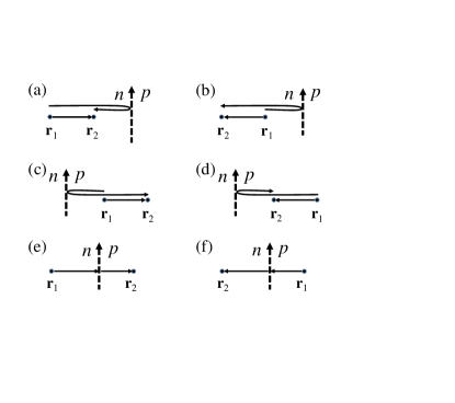
Figure 2: Piecewise construction of Green’s function (GF) $\mathbf{G}$ through intrinsic and scattering states. (a)/(b) $\mathbf{G}$ is the sum of intrinsic GF $\mathbf{G}_{0}$ constructed through right-going/left-going intrinsic states of the $\mathit{n}$ region), and extra GF constructed through the right-going intrinsic states and its left-going reflection states by the PNJ interface. (c)/(d) $\mathbf{G}$ is the sum of intrinsic GF $\mathbf{G}_{0}$ constructed through right-going/left-going intrinsic states of the $\mathit{p}$ region and extra GF constructed through the left-going intrinsic states and its right-going reflection states by the PNJ interface. (e)/(f) $\mathbf{G}$ is constructed through the right-going/left-going intrinsic states of the $\mathit{n}$/$\mathit{p}$ region and its right-going/left-going transmission states of the $\mathit{p}$/$\mathit{n}$ region.

Fig. 2 shows the piecewise construction of the GF $\mathbf{G}$ through the intrinsic and scattering states in the PNJ structure. The intrinsic state are the eigenstates of $\mathit{n}$ and $\mathit{p}$ regions in the PNJ while the scattering states are the renormalized eigenstates by the scattering coefficients. In Fig. 2, it is the interface of the PNJ leading to the scattering of incident intrinsic states. Considering the different incident states (maybe right-going or left-going) and the relative position of $\mathbf{r}_{1}$ and $\mathbf{r}_{2}$, there are total 6 pieces for the GF as shown by Fig. 2(a)-(f). To illustrate the operation of the construction technique, no loss of generality, we assume the right-going electron states incident from the left $\mathit{n}$ region of the PNJ, then the resulting states can be expressed as:

$$|\Psi(\mathbf{r})\rangle=\left\{\begin{array}[c]{ll}|\Psi_{\mathbf{k}_{\mathit{n},+}}(\mathbf{r})\rangle+r(k_{y})|\Psi_{\mathbf{k}_{\mathit{n},-}}(\mathbf{r})\rangle&(x<0),\\ t(k_{y})|\Psi_{\mathbf{k}_{\mathit{p},+}}(\mathbf{r})\rangle&(x>0).\end{array}\right.$$ (9)

Here, $\mathbf{k}_{\alpha,\pm}=(k_{\alpha,\pm,x},k_{y})$ are the right-going ($+$) and left-going ($-$) wave vectors in the $\alpha$ region, and the conservation of the tangential momentum $k_{y}$ has been used. For brevity, we omit the subscript $\lambda$ of the eigenstates since its value can be fully determined by the subscript $\alpha$ of the momentum through $\lambda=\mathrm{sgn}(\epsilon_{\alpha})$, and we also use this simplification to the pseudospin vector in the following. Since $k_{y}$ is conserved, the next step is to derive $k_{\alpha,\pm,x}$. By using the unitary matrix (cf. Eq. 6) for the vector transfromation between two coordinate systems, we have

$$k_{\alpha,\pm,x^{\prime}} =k_{\alpha,\pm,x}\cos\phi-k_{y}\sin\phi,$$ (10a)

$$k_{\alpha,\pm,y^{\prime}} =k_{\alpha,\pm,x}\sin\phi+k_{y}\cos\phi.$$ (10b)

Because $$\mathbf{k}_{\alpha,\pm}^{\prime}=(k_{\alpha,\pm,x^{\prime}},k_{\alpha,\pm,y^{\prime}})$$ satisfies Eq. 2 of eigenenergies, we obtain

$$Ak_{\alpha,\pm,x}^{2}+B_{\alpha}k_{\alpha,\pm,x}+C_{\alpha}=0,$$ (11)

where

$$A =\cos^{2}\phi+\gamma^{2}\sin^{2}\phi,$$ (12a)

$$B_{\alpha} =2\gamma_{2}\epsilon_{\alpha}\sin\phi-2(1-\gamma^{2})k_{y}\sin\phi\cos\phi,$$ (12b)

$$C_{\alpha} =k_{y}^{2}(\sin^{2}\phi+\gamma^{2}\cos^{2}\phi)+2\gamma_{2}\epsilon_{\alpha}k_{y}\cos\phi-\epsilon_{\alpha}^{2}.$$ (12c)

Here, $\gamma^{2}=\gamma_{1}^{2}-\gamma_{2}^{2}$ with $\gamma_{1}=v_{2}/v_{1}$ and $\gamma_{2}=v_{t}/v_{1}$, and $\epsilon_{\alpha}=\varepsilon_{\alpha}/v_{1}$ with $\varepsilon_{\mathit{n}}=E_{F}+V_{0}$ and $\varepsilon_{\mathit{p}}=E_{F}-V_{0}$. Eq. 11 is a quadratic equation with one unknown which gives two roots for $k_{\alpha,\pm,x}$:

$$k_{\alpha,\pm,x}=\frac{-B_{\alpha}\pm\sqrt{B_{\alpha}^{2}-4AC_{\alpha}}}{2A}.$$ (13)

So $k_{\alpha,\pm,x}$ is derived, and then $\mathbf{k}_{\alpha,\pm}^{\prime}$ is given by Eq. 10. And $r(k_{y})$ and $t(k_{y})$ are, respectively, reflection and transmission coefficients, which had been derived for the PNJ with a general junction directionZhang and Yang (2018):

$$r(k_{y}) =-\frac{\exp(i\theta_{\mathbf{S}({\mathbf{k}}_{\mathit{n},+})})-\exp(i\theta_{{\mathbf{S}}({\mathbf{k}}_{\mathit{p},+})})}{\exp(i\theta_{{\mathbf{S}}({\mathbf{k}}_{\mathit{n},-})})-\exp(i\theta_{{\mathbf{S}}({\mathbf{k}}_{\mathit{p},+})})},$$ (14a)

$$t(k_{y}) =\frac{\exp(i\theta_{{\mathbf{S}}({\mathbf{k}}_{\mathit{n},-})})-\exp(i\theta_{\mathbf{S}({\mathbf{k}}_{\mathit{n},+})})}{\exp(i\theta_{{\mathbf{S}}({\mathbf{k}}_{\mathit{n},-})})-\exp(i\theta_{{\mathbf{S}}({\mathbf{k}}_{\mathit{p},+})})}.$$ (14b)

Finally, GF can be constructed through the intrinsic and scattering state as the components of Eq. 9 for the resulting statesZhang et al. (2017b, a):

$$\mathbf{G}=\left\{\begin{array}[c]{ll}\mathbf{G}_{0}+\int dk_{y}\frac{r(k_{y})}{2\pi iv_{\mathit{n},x}}|\Psi_{\mathbf{k}_{\mathit{n},-}}(\mathbf{r}_{2})\rangle\langle\Psi_{\mathbf{k}_{\mathit{n},+}}(\mathbf{r}_{1})|&(x_{2}<0),\\ \int dk_{y}\frac{t(k_{y})}{2\pi iv_{\mathit{n},x}}|\Psi_{\mathbf{k}_{\mathit{p},+}}(\mathbf{r}_{2})\rangle\langle\Psi_{\mathbf{k}_{\mathit{n},+}}(\mathbf{r}_{1})|&(x_{2}>0).\end{array}\right.$$ (15)

Here, $v_{\mathit{n},x}\equiv v_{\mathit{n},x}(\mathbf{k}_{n,+})$ is the $x$ component of the group velocity $\mathbf{v}_{\mathit{n}}(\mathbf{k}_{\mathit{n},+})$ in the Cartesian coordinate system $x-y$. When $x_{2}<0$, Eq. 15 is the mathematical description of Fig. 2(a)/(b), which is the sum of intrinsic GF $\mathbf{G}_{0}$ constructed through right-going/left-going intrinsic states of the $\mathit{n}$ region (i.e., the free GF $\mathbf{G}_{0}$) and extra GF constructed through the right-going intrinsic states and its left-going reflection states by the PNJ interface. The free GF $\mathbf{G}_{0}\equiv\mathbf{G}_{0}(E_{F},\mathbf{r}_{2},\mathbf{r}_{1})$ is constructed completely by the intrinsic states and has the form:

$$\mathbf{G}_{0}=\int\frac{dk_{y}}{2\pi iv_{\mathit{n},x}}\left\{\begin{array}[c]{ll}|\Psi_{\mathbf{k}_{\mathit{n},+}}(\mathbf{r}_{2})\rangle\langle\Psi_{\mathbf{k}_{\mathit{n},+}}(\mathbf{r}_{1})|&(x_{2}>x_{1}),\\ |\Psi_{\mathbf{k}_{\mathit{n},-}}(\mathbf{r}_{2})\rangle\langle\Psi_{\mathbf{k}_{\mathit{n},-}}(\mathbf{r}_{1})|&(x_{2}<x_{1}).\end{array}\right.$$ (16)

which is consistent with the result derived through the straightforward Fourier transformation of the GF in momentum spaceZhang et al. (2019). When $x_{2}>0$, Eq. 15 is the mathematical description of Fig. 2(e), which is constructed through the right-going intrinsic states of the $\mathit{n}$ region and its right-going transmission states of the $\mathit{p}$ region. Most importantly, when $x_{2}>0$, we have $|\Psi_{\mathbf{k}_{\mathit{p},+}}(\mathbf{r}_{2})\rangle\langle\Psi_{\mathbf{k}_{\mathit{n},+}}(\mathbf{r}_{1})|\propto\exp(i\varphi_{\mathit{np}})$ where

$$\varphi_{\mathit{np}}(k_{y})=\mathbf{k}_{\mathit{p},+}\cdot\mathbf{r}_{2}-\mathbf{k}_{\mathit{n,+}}\cdot\mathbf{r}_{1}$$ (17)

is the propagation phase accumulated through the negative refraction of incident right-going intrinsic states in the $\mathit{n}$ region to become right-going transmission states in the $\mathit{p}$ regionZhang et al. (2017a). Similarly, to assume the left-going electron states incident from the right $\mathit{p}$ region of the PNJ, one can obtain the mathematical description of Fig. 2(c), (d) and (f). Noting here, the developed construction technique of GF is universal to the PNJ with a general junction direction.

III Results and discussions

In this section, we present the numerical results to display the negative refraction induced interference pattern of anisotropic and tilted MDFs across the 8-Pmmn borophene PNJ and discuss the underlying physics. No loss of generality, we focus on the GF matrix element $\left|{G}_{11}(E_{F},\mathbf{r}_{2},\mathbf{r}_{1})\right|$, since the interference pattern originates from the phase accumulation across the PNJ as shown in the following and has no qualitative difference among different GF matrix elements.

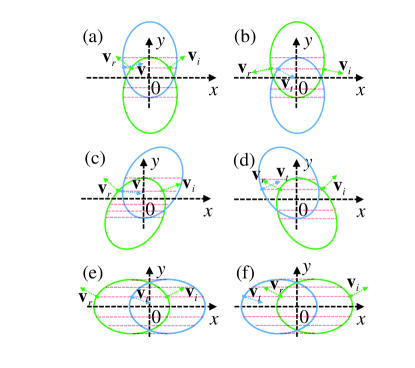
Figure 3: Dependence of momentum matching on the junction direction $\phi$. (a) $\phi=0$, (b) $\phi=\pi$, (c) $\phi=\pi/6$, (d) $\phi=-\pi/6$, (e) $\phi=\pi/2$, and (f) $\phi=-\pi/2$. The available states on the electron (green) and hole (blue) Fermi surfaces for the momentum matching subject to the conserved momentum $k_{y}$ as shown by the red dashed lines. The colored lines with arrows represent the group velocities ${\bf v}_{i,r,t}$ for the incident, reflection and transmission states, which are nonlinear with the conserved momenta. Here, we use $\varepsilon_{\mathit{n}}=\varepsilon_{\mathit{p}}=0.1$ as the doping configuration for p-n junctions.

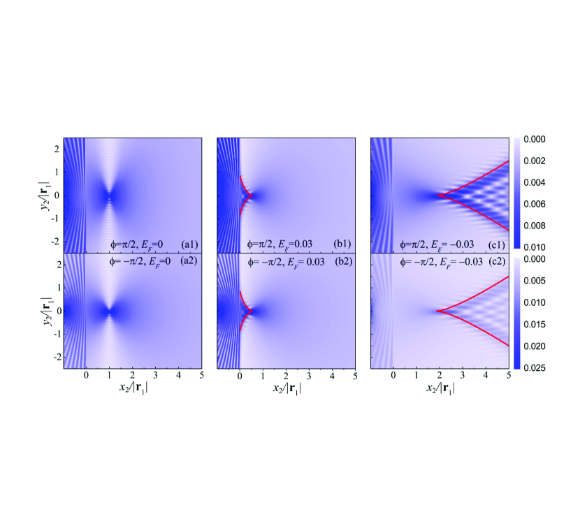
Figure 4: Veselago focusing and normal caustics in p-n junctions with junction directions parallel to $x^{\prime}$ axis shown by $\left|{G}_{11}(E_{F},\mathbf{r}_{2},\mathbf{r}_{1})\right|$. Two different junction directions (i.e., $\phi=\pm\pi/2$) and three different doping configurations (i.e., $E_{F}=0$, $\pm 0.03$) are considered. The red lines are the caustics from analytical formula. Here, $\mathbf{r}_{1}=(-200,0)$ and $V_{0}=0.1$.

Previous to the detailed calculations, we firstly present the intuitive physics for the interference pattern in 8-Pmmn borophene PNJ. In contrast to the isotropic MDFs across the graphene PNJCheianov et al. (2007), the anisotropy and tilt of MDFs should lead to the dependence of interference pattern on the junction direction of the 8-Pmmn borophene PNJ. The junction direction dependence implies the distinct momentum matching of states across borophene PNJ, then determines the appearance and the effectiveness of interference pattern. Fig. 3 shows the dependence of momentum matching on the junction direction $\phi$ of the borophene PNJ. Six typical junction directions are plotted, i.e., $\phi=0$, $\pi$, $\pm\pi/6$, and $\pm\pi/2$ as shown in Fig. 3(a)-(f). The available states on the electron (green) and hole (blue) Fermi surfaces for the momentum matching subject to the conserved momentum $k_{y}$ (cf. red dashed lines in Fig. 3). In Fig. 3, by assuming electron states incident from the left n region of the PNJ, we also plot the group velocities ${\bf v}_{i,r,t}$ for the right-going incident, left-going reflection and right-going transmission states. The noncollinear features between group velocities and conserved momenta are obvious. Comparing to the partial matching in Fig. 3(a)-(d), all states on the electron and hole Fermi surfaces may contribute to interference pattern in Fig. 3(e) and (f), then lead to the effective interference. More importantly, in Fig. 3(e) and (f), the electron and hole Fermi surfaces have the mirror symmetry about the junction interface, so Veselago focusing is expected in these two special junctionsZhang et al. (2016). As a representative interference pattern, Veselago focusing are studied intensively and are understood deeplyCheianov et al. (2007); Garcia-Pomar et al. (2008); Moghaddam and Zareyan (2010); Silveirinha and Engheta (2013); Zhao et al. (2013); Milovanovic et al. (2015); Bøggild et al. (2017); Zhang et al. (2017a); Hills et al. (2017). Therefore, the interference pattern in the special junctions with $\phi=\pm\pi/2$ being perpendicular to the tilt direction (namely, $y^{\prime}$ axis), can be as the starting point of our discussions. Then, we turn to the junctions with $\phi=0$ and $\phi=\pi$ (being parallel to the tilt direction) and the general junctions.

III.1 $\phi=\pm\pi/2$: Veselago focusing and normal caustics

We have picked out two special junctions perpendicular to the tilt direction (namely, $y^{\prime}$ axis) of MDFs in 8-Pmmn borophene. In these two special junctions, we plot the matrix element of GF $\left|{G}_{11}(E_{F},\mathbf{r}_{2},\mathbf{r}_{1})\right|$ in Fig. 4. For two different junction directions (i.e., $\phi=\pm\pi/2$), three different doping configurations are considered (i.e., $E_{F}=0$, $\pm 0.03$). For both special junctions, Veselago focusing as expectedZhang et al. (2016) (normal caustics very similar to that in graphene PNJCheianov et al. (2007)) appears when $E_{F}=0$ ($E_{F}=\pm 0.03$). For these two special junctions, we can analytically reveal the underlying physics of Veselago focusing and caustics. The tilt of MDFs in 8-Pmmn borophene leads to the breaking of mirror symmetry about the $x^{\prime}\$axis, so two cases of junction direction along $jx^{\prime}$ axis with $j=\pm$ are inequivalent (cf. momentum matching in Fig. 3(e) and (f)). For the junction direction along $jx^{\prime}$ direction, i.e., $\phi=-j\pi/2$, $\mathbf{k}_{\alpha,\pm}^{j}=(k_{\alpha,\pm,x}^{j},k_{y})$ has the form (cf. Eq. 13 for momentum components $k_{\alpha,\pm,x}^{j}$):

$$k_{\alpha,\pm,x}^{j}=\frac{1}{\gamma^{2}}(j\epsilon_{\alpha}\gamma_{2}\pm\lambda\sqrt{\epsilon_{\alpha}^{2}\gamma_{1}^{2}-\gamma^{2}k_{y}^{2}}).$$ (18)

Here, $\lambda=\mathrm{sgn}(\epsilon_{\alpha})$ conforms to Eq. 2 of eigenenergies. To show the formation of interference pattern of anisotropic and tilted MDFs across the PNJ, we examine the classical trajectory determined by the phase accumulation $\varphi_{\mathit{np}}$ (cf. Eq. 17). The classical trajectory with specific $k_{y,c}$ is determined by $\partial_{k_{y}}\varphi_{\mathit{np}}^{j}(k_{y})|_{k_{y,c}}=0$ asZhang et al. (2017a)

$$\partial_{k_{y}}k_{\mathit{p},+,x}^{j}x_{2}-\partial_{k_{y}}k_{\mathit{n},+,x}^{j}x_{1}+(y_{2}-y_{1})=0.$$ (19)

To differentiate Eq. 18, one can obtain

$$\partial_{k_{y}}k_{\mathit{n},+,x}^{j} =-\frac{k_{y}}{\sqrt{\gamma_{1}^{2}\epsilon_{n}^{2}-\gamma^{2}k_{y}^{2}}},$$ (20a)

$$\partial_{k_{y}}k_{\mathit{p},+,x}^{j} =\frac{k_{y}}{\sqrt{\gamma_{1}^{2}\epsilon_{p}^{2}-\gamma^{2}k_{y}^{2}}}.$$ (20b)

As a result, the classical trajectory with $$k_{y,c}$$ satisfies the equation:

$$y_{2}-y_{1}=-(\frac{k_{y,c}x_{2}}{\sqrt{\gamma_{1}^{2}\epsilon_{p}^{2}-\gamma^{2}k_{y,c}^{2}}}+\frac{k_{y,c}x_{1}}{\sqrt{\gamma_{1}^{2}\epsilon_{n}^{2}-\gamma^{2}k_{y,c}^{2}}}).$$ (21)

Noting here, Eq. 21 has no dependence on $j$, so it has the same form for two special junctions with $\phi=\pm\pi/2$. And Eq. 21 reproduces the result for isotropic MDFs when $v_{t}=0$ and $v_{1}=v_{2}$, i.e., $\gamma=\gamma_{1}=1$Zhang and Yang (2018).

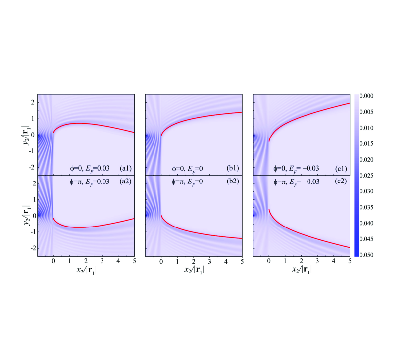
Figure 5: Anomalous caustics in PNJs with junction directions parallel to $y^{\prime}$ axis (i.e., $\phi=0$, $\pi$) shown by $\left|{G}_{11}(E_{F},\mathbf{r}_{2},\mathbf{r}_{1})\right|$. Three different Fermi levels ($E_{F}=0$, $\pm 0.03$) are considered. The red lines are the caustics from analytical formula. Here, $\mathbf{r}_{1}=(-200,0)$ and $V_{0}=0.1$.

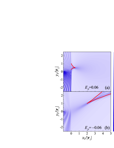
Figure 6: Same as Fig. 5 except that two higher magnitude of Fermi levels ($E_{F}=\pm 0.06$) are considered for $\phi=0$-junction.

III.1.1 Symmetric doping: Veselago focusing

To consider the symmetric doping, i.e., $E_{F}=0$ or $\epsilon_{n}=-\epsilon_{p}=V_{0}/v_{1}$, the classical trajectory is

$$y_{2}-y_{1}=-\frac{k_{y,c}(x_{2}+x_{1})}{\sqrt{\gamma_{1}^{2}\epsilon_{n}^{2}-\gamma^{2}k_{y,c}^{2}}}.$$ (22)

Obviously, when $x_{1}+x_{2}=0$ and $y_{2}=y_{1}$, Eq. 22 has no dependence on the momentum of classical trajectory, this implies that all classical trajectories from $\mathbf{r}_{1}=(x_{1},y_{1})$ converge to its mirror point $\mathbf{r}_{2}=(-x_{1},y_{1})$ about the junction interface, i.e., the appearance of Veselago focusing. Meanwhile, $k_{\mathit{n},+,x}^{j}=-k_{\mathit{p},+,x}^{j}$ and $\partial_{k_{y}}^{m}k_{\mathit{n},+,x}^{j}=-\partial_{k_{y}}^{m}k_{\mathit{p},+,x}^{j}$ with $m$ being a positive integer, so the zero-order term $\varphi_{\mathit{np}}^{j}(k_{y,c})=-k_{n,+,x}^{j}(x_{2}+x_{1})+k_{y,c}(y_{2}-y_{1})=0$ and the arbitrary order derivative of propagation phase $\varphi^{j}_{\mathit{np}}$ on the classical trajectory also vanishes identical to the case for isotropic MDFs in grapheneZhang and Yang (2018). However, noting that the different color scales for the Veselago focusing and caustics on the upper and bottom rows of Fig. 4, implying the different focusing magnitude. This reflects the inequivalence of two special junctions as mentioned previously, which has different density of states for the focusing states.

III.1.2 Asymmetric doping: normal caustics

To consider the asymmetric doping configuration (i.e., $E_{F}\neq 0$), Veselago focusing disappears, but the classical trajectories can form another kind of interference pattern (i.e., caustics) if the quadratic term  of $\varphi_{\mathit{np}}(k_{y})$ vanishesZhang and Yang (2018). Using Eq. 18, the vanishing quadratic term $\partial_{k_{y}^{2}}^{2}\varphi_{\mathit{np}}(k_{y})|_{k_{y,c}}=0$ leads to

$$\frac{\gamma_{1}^{2}\epsilon_{p}^{2}}{\left(\gamma_{1}^{2}\epsilon_{p}^{2}-\gamma^{2}k_{y,c}^{2}\right)^{\frac{3}{2}}}x_{2}+\frac{\gamma_{1}^{2}\epsilon_{n}^{2}}{\left(\gamma_{1}^{2}\epsilon_{n}^{2}-\gamma^{2}k_{y,c}^{2}\right)^{\frac{3}{2}}}x_{1}=0.$$ (23)

To solve the above equation, we derive

$$k_{y,c}^{2}=\frac{\gamma_{1}^{2}(c\epsilon_{n}^{2}-\epsilon_{p}^{2})}{(c-1)\gamma^{2}}$$ (24)

where $c=n^{2}(x_{2}/x_{\text{cump}})^{2/3}$ with $n=-\epsilon_{p}/\epsilon_{n}$ and $x_{\text{cump}}=-nx_{1}$. As a result, the classical trajectory is

$$y_{2}-y_{1} =\pm\frac{(x_{2}^{2/3}-x_{\text{cusp}}^{2/3})^{3/2}}{\gamma\sqrt{(n^{2}-1)}}\text{, for }n>1\text{ \& }x_{2}>x_{\text{cusp}},$$ (25a)

$$y_{2}-y_{1} =\pm\frac{(x_{\text{cusp}}^{2/3}-x_{2}^{2/3})^{3/2}}{\gamma\sqrt{1-n^{2}}}\text{, for }n<1\text{ \& }x_{2}<x_{\text{cusp}}.$$ (25b)

Eq. 25 reproduces the result for isotropic MDFs Zhang and Yang (2018) when $$\gamma=\gamma_{1}=1 v_{1}\neq v_{2} v_{t}\neq 0 \gamma\neq 1$$, and it just indicates the normal caustics. Due to the anisotropy () and tilt () of MDFs in 8-Pmmn borophene, leads to the modification of caustics. From a different perspective, this implies the tunability of caustics by changing the anisotropy and tilt of MDFs. In addition, the analytical Eq. 25 is used to plot the red lines in Fig. 4, and they are very consistent with the numerical results.

III.2 $\phi=0$ and $\pi$: anomalous caustics

Fig. 5 shows $\left|{G}_{11}(E_{F},\mathbf{r}_{2},\mathbf{r}_{1})\right|$ in PNJs with junction directions (i.e., $\phi=0$, $\pi$) parallel to tilt direction (namely $y^{\prime}$ axis). In Fig. 5, an outstanding feature is that the upper and bottom panels have the mirror symmetry about the $x$ axis. This comes from one hidden symmetry: To perform inversion operations $y\rightarrow-y$ and $k_{y}\rightarrow-k_{y}$ for $\phi$-junction, its momentum matching becomes the case of $(\pi-\phi)$-junction (cf. Fig. 3). Using this hidden symmetry, one can also explain the mirror symmetry of interference pattern about the $x$ axis in Fig. 4 since $\pi/2$-junction or $-\pi/2$-junction is symmetrically related to itself.

Comparing to Fig. 4 for special junctions, Veselago focusing does not exist and caustics becomes anomalous in Fig. 5, i.e., anomalous caustics. The MDFs in 8-Pmmn borophene have two features: anisotropy ($v_{1}\neq v_{2}$) and tilt ($v_{t}\neq 0$). To assume $v_{t}=0$, the electron and hole Fermi surfaces have the mirror symmetry about the PNJ interface when $E_{F}=0$, so Veselago focusing existsZhang et al. (2016, 2018). The absence of Veselago focusing in Fig. 5 is due to the breaking of mirror symmetry by the finite tilt (cf. Fig. 3(a) and (b)). Nevertheless, the anisotropy and tilt both contribute to the caustics, even in the special junctions (cf. Eq. 25). The $\phi$-dependent momentum matching further introduces the dependence of the anomalous caustics on the junction direction. For the junction direction along $jy^{\prime}$ direction, we have $\mathbf{k}_{\alpha,\pm}^{j}=(k_{\alpha,\pm,x}^{j},k_{y})$ and $k_{\alpha,\pm,x}^{j}$ are given by Eq. 13:

$$k_{\alpha,\pm,x}^{j}=\pm\lambda\sqrt{\epsilon_{\alpha}^{2}-k_{y}^{2}\gamma^{2}-2j\gamma_{2}\epsilon_{\alpha}k_{y}},$$ (26)

which implies

$$\partial_{k_{y}}k_{\mathit{n},+,x}^{j} =-\frac{k_{y}\gamma^{2}+j\gamma_{2}\epsilon_{n}}{\sqrt{-\gamma^{2}k_{y}^{2}+\epsilon_{n}^{2}-2j\gamma_{2}\epsilon_{n}k_{y}}},$$ (27a)

$$\partial_{k_{y}}k_{\mathit{p},+,x}^{j} =\frac{k_{y}\gamma^{2}+j\gamma_{2}\epsilon_{p}}{\sqrt{-\gamma^{2}k_{y}^{2}+\epsilon_{p}^{2}-2j\gamma_{2}\epsilon_{p}k_{y}}}.$$ (27b)

Using Eq. 17, the vanishing quadratic term $$\partial_{k_{y}^{2}}^{2}\varphi_{\mathit{np}}(k_{y})|_{k_{y,c}}=0$$ leads to

$$\frac{\epsilon_{p}^{2}x_{2}}{\left(-\gamma^{2}k_{y}^{2}+\epsilon_{p}^{2}-2j\gamma_{2}\epsilon_{p}k_{y}\right)^{\frac{3}{2}}}=\frac{-\epsilon_{n}^{2}x_{1}}{\left(-\gamma^{2}k_{y}^{2}+\epsilon_{n}^{2}-2j\gamma_{2}\epsilon_{n}k_{y}\right)^{\frac{3}{2}}}.$$ (28)

The solution of the above equation is

$$k_{y,c}^{j}=\frac{-j\gamma_{2}(c\epsilon_{n}-\epsilon_{p})\pm\sqrt{(\gamma_{2}^{2}c\epsilon_{n}-\epsilon_{p})^{2}-\gamma^{2}(c-1)(\epsilon_{p}^{2}-c\epsilon_{n}^{2})}}{(c-1)\gamma^{2}}.$$ (29)

Substituting Eqs. 27 and 29 into Eq. 19, the anomalous caustics can be determined and is shown by the red lines in Fig. 5. The analytical and numerical results agree very well with each other.

In addition, Fig. 5 also shows the dependence of anomalous caustics on the doping configuration. With decreasing $E_{F}$ from left to right on the upper (bottom) row, the anomalous caustics goes upward (downward). This implies the tunable anomalous caustics by doping configuration. It attracts us to further increase the magnitude of $E_{F}$ to examine the interference pattern. Fig. 6 shows the interference pattern of $\left|{G}_{11}(E_{F},\mathbf{r}_{2},\mathbf{r}_{1})\right|$ same as Fig. 5 except that two higher magnitude of Fermi levels ($E_{F}=\pm 0.06$) are considered for ($\phi=0$)-junction. On the caustics, Fig. 5 has a single branch, whereas there are two branches in Fig. 6. In the sense of the same branch number for caustics in Fig. 4 and Fig. 6, the anomalous feature is suppressed by the high value of $E_{F}$. And there should be one critical $E_{F}$ at which the anomalous caustics changes its branch number. In all, the anomalous caustics has a strong dependence on doping configuration and exhibits rich patterns.

III.3 General $\phi$: anomalous caustics

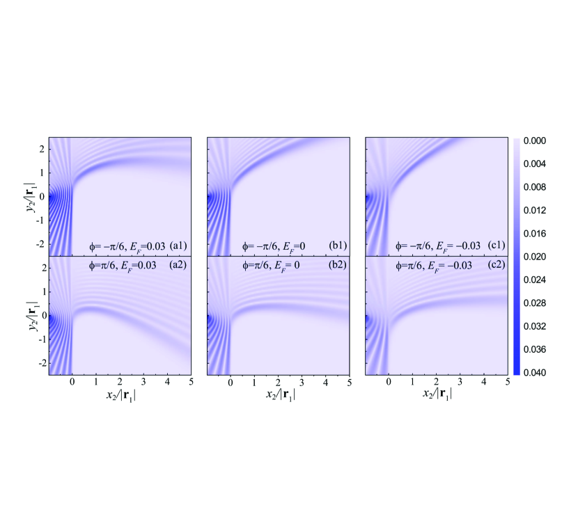
Figure 7: Anomalous caustics in the PNJ with general junction directions shown by $\left|{G}_{11}(E_{F},\mathbf{r}_{2},\mathbf{r}_{1})\right|$. Two different junction directions (i.e., $\phi=\pm\pi/6$) and three different Fermi levels (i.e., $E_{F}=0$, $\pm 0.03$) are considered.

In general cases, the junction directions $\phi$ of PNJs are neither perpendicular nor parallel to the tilt direction of MDFs in 8-Pmmn borophene. It is rather difficult to examine the transport properties of these general $\phi$-junctions, because their low symmetry requires large unit cell to perform numerical simulation, e.g., through the recursive GF based on the lattice HamiltonianLow and Appenzeller (2009). By using the developed construction technique of GF in Sec. IIB, the transport problem in general $\phi$-junctions can be solved efficiently. Fig. 7 shows $\left|{G}_{11}(E_{F},\mathbf{r}_{2},\mathbf{r}_{1})\right|$ by considering two different junction directions (i.e., $\phi=\pm\pi/6$) and three different Fermi levels (i.e., $E_{F}=0$, $\pm 0.03$). In light of the mirror symmetry about the $x$ axis for $\phi$-junction and $(\pi-\phi)$-junction, one only needs to explicitly discuss the junction directions $\phi\in[-\pi/2,\pi/2]$, so $\phi=\pm\pi/6$ are typical enough. Fig. 7 is very similar to Fig. 5, featured by the anomalous caustics. And with decreasing $E_{F}$ from left to right on the upper or bottom row, the anomalous caustics goes upward. Therefore, the anomalous caustics depends strongly on the junction directions and doping configuration, favoring its tunability.

IV Conclusions

In summary, we investigate the negative refraction induced interference of anisotropic and tilted MDFs across 8-Pmmn borophene PNJs. Because of the anisotropy and tilt, the calculation of GF of the PNJ with an arbitrary junction direction is needed, for which we develop an effective construction technique. The developed construction technique of GF can be generalized to study the transport of other novel MDFs, e.g., type-II Dirac fermionsLu et al. (2016b); Milićević et al. (2019), and semi-Dirac fermions Banerjee et al. (2009). Comparing to the seminal workCheianov et al. (2007), here we focus negative refraction induced Veselago focusing and caustics. If the junction direction is perpendicular to the tilt direction of MDFs, Veselago focusing or normal caustics appears resting on the doping configuration of the PNJ. More importantly, to the other junction, we discover one new phenomenon, i.e., anomalous caustics, which can be manipulated by junction direction and doping configuration. The interference pattern is unique to anisotropic and tilted MDFs, which is demonstrated numerically and analytically. This model study is generally applicable to the ideal p-n junctions with perfect border, while the imperfect border (e.g., the disorder-induced losses and smooth junctions) will lead to the diffusive scattering and reduce the transmission of electrons across the electrons. To implement the Dirac fermions into electron optics, people make a great effort to improve the experimental fabrication of ideal p-n junction. For example, very ideal atomically sharp p-n junction have been created Bai et al. (2018); Zhou et al. (2019); Chaves et al. (2019). In addition, with the rapid experimental advance of borophene Mannix et al. (2015); Feng et al. (2016, 2017); Wang et al. (2019) and the demonstration of negation refraction Lee et al. (2015); Chen et al. (2016b); Brun et al. (2019), we expect the anomalous caustics to be observable in the near future, then this study make novel MDFs (e.g., in 8-Pmmn borophene) promising to engineer Dirac electron optics devices.

References

- Pendry (2000) J. B. Pendry, Phys. Rev. Lett. 85, 3966 (2000).
- Smith et al. (2004) D. R. Smith, J. B. Pendry, and M. C. K. Wiltshire, Science 305, 788 (2004).
- Chen et al. (2016a) H.-T. Chen, A. J. Taylor, and N. Yu, Reports on Progress in Physics 79, 076401 (2016a).
- Castro Neto et al. (2009) A. H. Castro Neto, F. Guinea, N. M. R. Peres, K. S. Novoselov, and A. K. Geim, Rev. Mod. Phys. 81, 109 (2009).
- Low (2012) T. Low, Graphene pn Junction: Electronic Transport and Devices (Springer Berlin Heidelberg, Berlin, Heidelberg, 2012), pp. 467–508.
- Frisenda et al. (2018) R. Frisenda, A. J. Molina-Mendoza, T. Mueller, A. Castellanos-Gomez, and H. S. J. van der Zant, Chem. Soc. Rev. 47, 3339 (2018).
- Cheianov et al. (2007) V. V. Cheianov, V. Fal’ko, and B. L. Altshuler, Science 315, 1252 (2007).
- Lee et al. (2015) G.-H. Lee, G.-H. Park, and H.-J. Lee, Nat. Phys. 11, 925 (2015).
- Chen et al. (2016b) S. Chen, Z. Han, M. M. Elahi, K. M. M. Habib, L. Wang, B. Wen, Y. Gao, T. Taniguchi, K. Watanabe, J. Hone, et al., Science 353, 1522 (2016b).
- Garcia-Pomar et al. (2008) J. L. Garcia-Pomar, A. Cortijo, and M. Nieto-Vesperinas, Phys. Rev. Lett. 100, 236801 (2008).
- Moghaddam and Zareyan (2010) A. G. Moghaddam and M. Zareyan, Phys. Rev. Lett. 105, 146803 (2010).
- Silveirinha and Engheta (2013) M. G. Silveirinha and N. Engheta, Phys. Rev. Lett. 110, 213902 (2013).
- Zhao et al. (2013) L. Zhao, P. Tang, B.-L. Gu, and W. Duan, Phys. Rev. Lett. 111, 116601 (2013).
- Milovanovic et al. (2015) S. P. Milovanovic, D. Moldovan, and F. M. Peeters, J. Appl. Phys. 118, 154308 (2015).
- Bøggild et al. (2017) P. Bøggild, J. M. Caridad, C. Stampfer, G. Calogero, N. R. Papior, and M. Brandbyge, Nature Communications 8, 15783 (2017).
- Zhang et al. (2017a) S.-H. Zhang, J.-J. Zhu, W. Yang, and K. Chang, 2D Materials 4, 035005 (2017a).
- Hills et al. (2017) R. D. Y. Hills, A. Kusmartseva, and F. V. Kusmartsev, Phys. Rev. B 95, 214103 (2017).
- Zhang et al. (2018) S.-H. Zhang, W. Yang, and F. M. Peeters, Phys. Rev. B 97, 205437 (2018).
- Betancur-Ocampo (2018) Y. Betancur-Ocampo, Phys. Rev. B 98, 205421 (2018).
- Prabhakar et al. (2019) S. Prabhakar, R. Nepal, R. Melnik, and A. A. Kovalev, Phys. Rev. B 99, 094111 (2019).
- Brun et al. (2019) B. Brun, N. Moreau, S. Somanchi, V.-H. Nguyen, K. Watanabe, T. Taniguchi, J.-C. Charlier, C. Stampfer, and B. Hackens, Phys. Rev. B 100, 041401 (2019).
- Wehling et al. (2014) T. Wehling, A. Black-Schaffer, and A. Balatsky, Advances in Physics 63, 1 (2014).
- Wang et al. (2015) J. Wang, S. Deng, Z. Liu, and Z. Liu, National Science Review 2, 22 (2015).
- Xu et al. (2018) R. Xu, X. Zou, B. Liu, and H.-M. Cheng, Materials Today 21, 391 (2018).
- Milićević et al. (2019) M. Milićević, G. Montambaux, T. Ozawa, O. Jamadi, B. Real, I. Sagnes, A. Lemaître, L. Le Gratiet, A. Harouri, J. Bloch, et al., Phys. Rev. X 9, 031010 (2019).
- Goerbig et al. (2008) M. O. Goerbig, J.-N. Fuchs, G. Montambaux, and F. Piéchon, Phys. Rev. B 78, 045415 (2008).
- Lu et al. (2016a) H.-Y. Lu, A. S. Cuamba, S.-Y. Lin, L. Hao, R. Wang, H. Li, Y. Zhao, and C. S. Ting, Phys. Rev. B 94, 195423 (2016a).
- Zhou et al. (2014) X.-F. Zhou, X. Dong, A. R. Oganov, Q. Zhu, Y. Tian, and H.-T. Wang, Phys. Rev. Lett. 112, 085502 (2014).
- Lopez-Bezanilla and Littlewood (2016) A. Lopez-Bezanilla and P. B. Littlewood, Phys. Rev. B 93, 241405 (2016).
- Zabolotskiy and Lozovik (2016) A. D. Zabolotskiy and Y. E. Lozovik, Phys. Rev. B 94, 165403 (2016).
- Nakhaee et al. (2018) M. Nakhaee, S. A. Ketabi, and F. M. Peeters, Phys. Rev. B 97, 125424 (2018).
- Cheng et al. (2017) T. Cheng, H. Lang, Z. Li, Z. Liu, and Z. Liu, Phys. Chem. Chem. Phys. 19, 23942 (2017).
- Sadhukhan and Agarwal (2017) K. Sadhukhan and A. Agarwal, Phys. Rev. B 96, 035410 (2017).
- Jalali-Mola and Jafari (2018) Z. Jalali-Mola and S. A. Jafari, Phys. Rev. B 98, 235430 (2018).
- Verma et al. (2017) S. Verma, A. Mawrie, and T. K. Ghosh, Phys. Rev. B 96, 155418 (2017).
- Islam and Jayannavar (2017) S. F. Islam and A. M. Jayannavar, Phys. Rev. B 96, 235405 (2017).
- Zhang and Yang (2018) S.-H. Zhang and W. Yang, Phys. Rev. B 97, 235440 (2018).
- Champo and Naumis (2019) A. E. Champo and G. G. Naumis, Phys. Rev. B 99, 035415 (2019).
- Paul et al. (2019) G. C. Paul, S. F. Islam, and A. Saha, Phys. Rev. B 99, 155418 (2019).
- Zhang et al. (2019) S.-H. Zhang, D.-F. Shao, and W. Yang, Journal of Magnetism and Magnetic Materials 491, 165631 (2019).
- Zhang et al. (2017b) S.-H. Zhang, W. Yang, and K. Chang, Phys. Rev. B 95, 075421 (2017b).
- Sakurai (1994) J. J. Sakurai, Modern Quantum Mechanics (Revised Edition) (Addison-Wesley Publishing Company, Inc., 1994).
- Griffiths (1995) D. J. Griffiths, Introduction to Quantum Mechanics (Prentice Hall, Upper Saddle River, New Jersey 07458, 1995).
- Cohen-Tannoudji et al. (2005) C. Cohen-Tannoudji, B. Diu, and F. Laloe, Quantum Mechanics vol 2, 2nd ed (Wiley-VCH, New York, 2005).
- Zhang et al. (2016) S.-H. Zhang, J.-J. Zhu, W. Yang, H.-Q. Lin, and K. Chang, Phys. Rev. B 94, 085408 (2016).
- Low and Appenzeller (2009) T. Low and J. Appenzeller, Phys. Rev. B 80, 155406 (2009).
- Lu et al. (2016b) Y. Lu, D. Zhou, G. Chang, S. Guan, W. Chen, Y. Jiang, J. Jiang, X.-s. Wang, S. A. Yang, Y. P. Feng, et al., npj Computational Materials 2, 16011 (2016b).
- Banerjee et al. (2009) S. Banerjee, R. R. P. Singh, V. Pardo, and W. E. Pickett, Phys. Rev. Lett. 103, 016402 (2009).
- Bai et al. (2018) K.-K. Bai, J.-J. Zhou, Y.-C. Wei, J.-B. Qiao, Y.-W. Liu, H.-W. Liu, H. Jiang, and L. He, Phys. Rev. B 97, 045413 (2018).
- Zhou et al. (2019) X. Zhou, A. Kerelsky, M. M. Elahi, D. Wang, K. M. M. Habib, R. N. Sajjad, P. Agnihotri, J. U. Lee, A. W. Ghosh, F. M. Ross, et al., ACS Nano 13, 2558 (2019).
- Chaves et al. (2019) F. A. Chaves, D. Jim nez, J. E. Santos, P. B?ggild, and J. M. Caridad, Nanoscale 11, 10273 (2019).
- Mannix et al. (2015) A. J. Mannix, X.-F. Zhou, B. Kiraly, J. D. Wood, D. Alducin, B. D. Myers, X. Liu, B. L. Fisher, U. Santiago, J. R. Guest, et al., Science 350, 1513 (2015).
- Feng et al. (2016) B. Feng, J. Zhang, Q. Zhong, W. Li, S. Li, H. Li, P. Cheng, S. Meng, L. Chen, and K. Wu, Nature Chemistry 8, 563 (2016).
- Feng et al. (2017) B. Feng, O. Sugino, R.-Y. Liu, J. Zhang, R. Yukawa, M. Kawamura, T. Iimori, H. Kim, Y. Hasegawa, H. Li, et al., Phys. Rev. Lett. 118, 096401 (2017).
- Wang et al. (2019) Z.-Q. Wang, T.-Y. Lü, H.-Q. Wang, Y. P. Feng, and J.-C. Zheng, Frontiers of Physics 14, 33403 (2019).