The electromagnetic form factors of the transition from the spin-3/2 Sigma to the Lambda hyperon

Abstract

The three electromagnetic form factors for the transition from a $3/2^{+}$ $\Sigma^{*}$ hyperon to the ground-state $\Lambda$ hyperon are studied. At low energies, combinations of the transition form factors can be deduced from Dalitz decays of the $\Sigma^{*}$ hyperon to $\Lambda$ plus an electron-positron pair. It is pointed out how more information can be obtained with the help of the self-analyzing weak decay of the $\Lambda$. In particular it is shown that these transition form factors are complex quantities already in this kinematical region. Such measurements are feasible at hyperon factories as for instance the Facility for Antiproton and Ion Research (FAIR). At higher energies, the transition form factors can be measured in electron-positron collisions. The pertinent relations between the transition form factors and the decay distributions and differential cross sections are presented. Using dispersion theory, the low-energy electromagnetic form factors for the $\Sigma^{*}$-to-$\Lambda$ transition are related to the pion vector form factor. The additionally required input, i.e. the two-pion–$\Sigma^{*}$–$\Lambda$ amplitudes are determined from relativistic next-to-leading-order (NLO) baryon chiral perturbation theory including the baryons from the octet and the decuplet. A poorly known NLO parameter is fixed to the experimental value of the $\Sigma^{*}\to\Lambda\gamma$ decay width. Pion rescattering is taken into account by dispersion theory solving a Muskhelishvili-Omnès equation. Subtracted and unsubtracted dispersion relations are discussed. However, in view of the fact that the transition form factors are complex quantities, the current data situation does not allow for a full determination of the subtraction constants. To reduce the number of free parameters, unsubtracted dispersion relations are used to make predictions for the transition form factors in the low-energy space- and timelike regions.

I Introduction and summary

Electromagnetic form factors have become an important tool to study the structure of strongly interacting objects, see e.g. Landsberg (1985); Czerwiński et al. (2012); Miller (2007); Punjabi et al. (2015); Körner and Kuroda (1977); Carlson (1986); Pascalutsa et al. (2007); Kaxiras et al. (1985); Kubis and Meißner (2001); Ablikim et al. (2019); Granados et al. (2017); Alarcón et al. (2017) and references therein. Depending on the invariant mass of the virtual photon, one achieves different resolutions and different degrees of freedom become relevant. At very large energies, one “sees” the minimal quark content of the probed object Brodsky and Farrar (1975); Lepage and Brodsky (1979); Carlson (1986). Asymptotic freedom causes a suppression of the influence of any non-minimal quark or gluon content of the probed state. At low energies, the dynamics of pions has an important influence on the shape of form factors. Dynamical chiral symmetry breaking causes the appearance of Goldstone bosons Scherer and Schindler (2012), the pions. Because they are much lighter than any other hadron, pions can be excited with energies so low that all other degrees of freedom are still frozen. Both aspects, dominance of minimal quark content at high energies and universal pion dynamics at low energies, are model-independent consequences of Quantum Chromodynamics (QCD). A complete description of a form factor must include both of these aspects.

The purpose of Granados et al. (2017) and of the present and future work is to provide the low-energy input for such a complete description of form factors in the hyperon sector. Here we extend previous work of the Uppsala group Granados et al. (2017); Leupold (2018) where dispersion theory is used to relate in a model-independent way isovector form factors of baryons to pion-baryon scattering amplitudes. In a second step, these scattering amplitudes are approximated by relativistic chiral perturbation theory ($\chi$PT) including the baryon octet and decuplet as active degrees of freedom. Conceptually this is close in spirit to Alarcón et al. (2017); Alarcón and Weiss (2017, 2018a, 2018b). On a more technical level, the rescattering of pions is treated differently in Alarcón et al. (2017) and in Granados et al. (2017). In Alarcón et al. (2017) an N/D method is used; in Granados et al. (2017) a Muskhelishvili-Omnès (MO) equation is solved. As has been demonstrated in Leupold (2018) for the nucleon case, solving an MO equation with input from $\chi$PT up to next-to-leading order leads to better results when compared to a fully dispersive calculation Hoferichter et al. (2016a, b). For the case of hyperons, the use of dispersively reconstructed pion-baryon amplitudes is not an option because there are no direct data on pion-hyperon scattering. Therefore, we rely also in the present work on input from $\chi$PT Jenkins and Manohar (1991); Dashen and Manohar (1993); Pascalutsa et al. (2007); Ledwig et al. (2014); Holmberg and Leupold (2018) and solve an MO equation. A combined use of dispersion theory and $\chi$PT has been pioneered in Donoghue et al. (1990); see also Donoghue (1996) for a brief review.

A general motivation for studying hyperon form factors has been provided in Granados et al. (2017) in great detail. With the present work, we extend the approach of Granados et al. (2017) to electromagnetic form factors of hyperons with spin 3/2. Our framework is suited for the determination of isovector form factors. Therefore we focus in the present work on the only electromagnetic form factors of hyperons that are purely isovector (and involve a spin 3/2 state). These are the form factors for the transition of the lowest lying spin 3/2 decuplet state $\Sigma^{*0}$ to the spin 1/2 ground state $\Lambda$.

In the timelike region, these transition form factors (TFFs) can be measured at low energies via the Dalitz decay $\Sigma^{*0}\to\Lambda\,e^{+}e^{-}$. It can be expected that these Dalitz decays will be addressed in the near future by the collaborations HADES Ramstein et al. (2019) and PANDA Lutz et al. (2009) at the Facility for Antiproton and Ion Research (FAIR). Therefore we regard our present work as very timely.

Concerning the $\Sigma^{*}$-$\Lambda$ transition, two distinct qualitative aspects are noteworthy; one is more case specific, one is universal. We start with the latter. Whenever pions are excited, they rescatter. In the isovector channel, the p-wave pion phase shift shows a relatively broad, essentially elastic resonance, the $\rho$ meson Colangelo et al. (2001); Garcia-Martin et al. (2011). Thus, the universal pion dynamics gives rise to the coupling of the virtual photon to the $\rho$-meson. Phenomenologically, this is covered by the concept of vector meson dominance Sakurai (1969). In the dispersive framework this is covered by the pion phase shift and the pion vector form factor. We will explore the quantitative importance of these effects in the present paper.

There is a second aspect, however, which is also covered by our dispersive framework, but is typically missing in a vector meson dominance approach. This is the aspect that we called “more case specific”. Being resonances, the $\Sigma^{*}$ hyperons are unstable. In particular, the $\Sigma^{*0}$ can decay to $\Sigma^{\pm}\,\pi^{\mp}$. This pair can rescatter into a $\Lambda$ and a real or virtual photon. Therefore, the TFFs are complex quantities in all kinematically allowed regimes: in the spacelike scattering region of $\Sigma^{*0}\,e^{-}\leftrightarrow\Lambda\,e^{-}$; at the photon point $\Sigma^{*0}\to\Lambda\,\gamma$; in the low-energy timelike Dalitz decay region of $\Sigma^{*0}\to\Lambda\,e^{+}e^{-}$; and in the high-energy production region of $e^{+}e^{-}\to\Sigma^{*0}\,\bar{\Lambda}$. This is in contrast to TFFs for hadrons that are stable with respect to the strong interaction. For stable hadrons, the TFFs are essentially real in all regimes except for the production region.

Complex form factors allow for non-trivial interference patterns between them. Those can be measured, e.g., with the help of the self-analyzing weak decays of the “stable” hyperons. In practice, this means that in the succession of the two decays $\Sigma^{*0}\to\Lambda\,e^{+}e^{-}$ and $\Lambda\to p\,\pi^{-}$, the angular distribution of the second decay contains interesting information about the interference of the TFFs. This information is accessible without involving the production process or the spin orientation of the $\Sigma^{*0}$ and without determining the spin orientation of the proton Fäldt (2016); Perotti et al. (2019). On the other hand, in a strict vector meson dominance scenario, the $\Sigma^{*0}$ couples just via a pointlike interaction to $\rho\,\Lambda$. There, a form factor can only become complex where the $\rho$ becomes unstable. This happens essentially only above the two-pion threshold. But in the Dalitz decay region of $\Sigma^{*0}\to\Lambda\,e^{+}e^{-}$, the maximally possible dielectron invariant mass (“$\rho$-meson invariant mass”) is $m_{\Sigma^{*}}-m_{\Lambda}<2m_{\pi}$ Tanabashi et al. (2018). Thus in reality, the TFFs are complex but in a simple vector meson dominance approach they are real in the Dalitz decay region. We will also explore the quantitative importance of these effects. One peculiarity we observe is that even if the imaginary part of a TFF at the photon point is very small, it gets larger for the transition radius.

Ideally we would like to use subtracted dispersion relations, but the available experimental input is too scarce to allow for it. For the case at hand there are three TFFs and therefore three complex valued subtraction constants. For the time being we choose to use unsubtracted dispersion relations; being aware of the large uncertainties they carry, we still expect to obtain results of the correct order of magnitude.

In the first part of the paper we define the $\Sigma^{*0}$-$\Lambda$ TFFs and relate them to several observables, accessible in different kinematical regions. Directly after we enter the core of the theoretical work: we derive the appropriate dispersion relations for pion-hyperon scattering amplitudes and TFFs. Finally the results are presented. There are several appendices with various purposes. Appendix A clarifies how the individual contributions of meson and baryon dynamics influence the final results. The others complement the main text with technical details.

II Transition form factors and observables

Following essentially Körner and Kuroda (1977) we define three TFFs via

$$\langle 0|j_{\mu}|\Sigma^{*}\bar{\Lambda}\rangle=e\,\bar{v}_{\Lambda}(p_{\Lambda},\lambda)\,\Gamma_{\mu\nu}(p_{\Sigma^{*}},p_{\Lambda})\,u_{\Sigma^{*}}^{\nu}(p_{\Sigma^{*}},\sigma)$$ (1)

with

$$\Gamma^{\mu\nu}(p_{\Sigma^{*}},p_{\Lambda}) := -(\gamma^{\mu}q^{\nu}-\not\!q\,g^{\mu\nu})\,m_{\Sigma^{*}}\,\gamma_{5}\,F_{1}(q^{2})$$ (2)

$${}+(p_{\Sigma^{*}}^{\mu}q^{\nu}-p_{\Sigma^{*}}\cdot q\,g^{\mu\nu})\,\gamma_{5}\,F_{2}(q^{2})$$

$${}+(q^{\mu}q^{\nu}-q^{2}\,g^{\mu\nu})\,\gamma_{5}\,F_{3}(q^{2})$$

and $q:=p_{\Sigma^{*}}+p_{\Lambda}$. Conventions for the spin-3/2 spinor $u^{\mu}$ are provided in Appendix B. The neutral spin-3/2 Sigma hyperon is denoted by $\Sigma^{*}$. The helicities (not spins!) of $\Sigma^{*}$ and $\bar{\Lambda}$ are called $\sigma$ and $\lambda$, respectively.

The TFFs defined via (1) are appropriate for a dispersive representation where we study formally the reaction $\Sigma^{*}\bar{\Lambda}\to\pi^{+}\pi^{-}\to\gamma^{*}$. Physically, however, we study the reactions $e^{+}e^{-}\to\gamma^{*}\to\bar{\Sigma}^{*}\Lambda$ and $\Sigma^{*}\to\Lambda\,\gamma^{*}\to\Lambda\;e^{+}e^{-}$. In addition, if one wants to compare the results of the electromagnetic form factors for the transition $\Sigma^{*}\to\Lambda$ with the ones for $\Delta\to N$ it is convenient to adapt to the conventions used in the $\Delta$ sector where mostly electroproduction is studied Carlson (1986); Pascalutsa et al. (2007) and not Dalitz decays. Thus one should also look at the reaction $e^{-}\Lambda\to e^{-}\Sigma^{*}$ or more formally $\Lambda\,\gamma^{*}\to\Sigma^{*}$. Therefore we present the transition form factors also for other kinematical regimes.

In principle, the reactions $\Sigma^{*}\bar{\Lambda}\to\gamma^{*}$, $\gamma^{*}\to\bar{\Sigma}^{*}\Lambda$ and $\Sigma^{*}\to\Lambda\,\gamma^{*}$ are related by crossing symmetry. For $\Lambda\,\gamma^{*}\to\Sigma^{*}$ one might involve charge conjugation and then again crossing symmetry.

For the amplitude relevant for the Dalitz decay, $\Sigma^{*}\to\Lambda\,\gamma^{*}$, one finds

$$\langle\Lambda|j_{\mu}|\Sigma^{*}\rangle=e\,\bar{u}_{\Lambda}(p_{\Lambda},\lambda)\,\Gamma_{\mu\nu}(p_{\Sigma^{*}},-p_{\Lambda})\,u_{\Sigma^{*}}^{\nu}(p_{\Sigma^{*}},\sigma)\,.$$ (3)

In practice this leads to the very same expression as on the right-hand side of (2) but with $q:=p_{\Sigma^{*}}-p_{\Lambda}$.

For the production amplitude $\gamma^{*}\to\bar{\Sigma}^{*}\Lambda$ one has to specify the meaning of the two-fermion bra state:

$$\langle\bar{\Sigma}^{*}\Lambda|:=|\bar{\Sigma}^{*}\Lambda\rangle^{\dagger}\,.$$ (4)

The structure corresponding to (2) would be $\Gamma^{\mu\nu}(-p_{\Sigma^{*}},-p_{\Lambda})$, but it is not convenient to define $q$ as $-p_{\Sigma^{*}}-p_{\Lambda}$. Therefore we rather provide a fully explicit version of the TFFs adapted to the production process:

$$\langle\bar{\Sigma}^{*}\Lambda|j_{\mu}|0\rangle=-e\,\bar{u}_{\Lambda}(p_{\Lambda},\lambda)\,\tilde{\Gamma}_{\mu\nu}(p_{\Sigma^{*}},p_{\Lambda})\,v_{\Sigma^{*}}^{\nu}(p_{\Sigma^{*}},\sigma)\,,$$ (5)

$$\tilde{\Gamma}^{\mu\nu}(p_{\Sigma^{*}},p_{\Lambda}) := (\gamma^{\mu}q^{\nu}-\not\!q\,g^{\mu\nu})\,m_{\Sigma^{*}}\,\gamma_{5}\,F_{1}(q^{2})$$ (6)

$${}+(p_{\Sigma^{*}}^{\mu}q^{\nu}-p_{\Sigma^{*}}\cdot q\,g^{\mu\nu})\,\gamma_{5}\,F_{2}(q^{2})$$

$${}+(q^{\mu}q^{\nu}-q^{2}\,g^{\mu\nu})\,\gamma_{5}\,F_{3}(q^{2})$$

with $q:=p_{\Sigma^{*}}+p_{\Lambda}$.

Finally we obtain for the excitation process:

$$\langle\Sigma^{*}|j_{\mu}|\Lambda\rangle=-e\,\bar{u}_{\Sigma^{*}}^{\nu}(p_{\Sigma^{*}},\sigma)\,\tilde{\Gamma}_{\mu\nu}(p_{\Sigma^{*}},-p_{\Lambda})\,u_{\Lambda}(p_{\Lambda},\lambda)\,.$$ (7)

Here the pertinent expression for $\tilde{\Gamma}^{\mu\nu}$ agrees with the right-hand side of (6) provided one defines $q:=p_{\Sigma^{*}}-p_{\Lambda}$.

Next we introduce linear combinations of $F_{1}$, $F_{2}$ and $F_{3}$, which correspond to TFFs with fixed helicity combinations. We denote them by $G_{m}$ ($m=\sigma-\lambda=0,\pm 1$) and find:

$$G_{-1}(q^{2}) := (-m_{\Lambda}(m_{\Lambda}+m_{\Sigma^{*}})+q^{2})\,F_{1}(q^{2})$$ (8)

$${}+\frac{1}{2}\,(m_{\Sigma^{*}}^{2}-m_{\Lambda}^{2}+q^{2})\,F_{2}(q^{2})+q^{2}\,F_{3}(q^{2})$$

$$\mbox{for}\quad\sigma=-\frac{1}{2}\,,\lambda=+\frac{1}{2}\,,$$

$$G_{0}(q^{2}) := m^{2}_{\Sigma^{*}}\,F_{1}(q^{2})+m^{2}_{\Sigma^{*}}\,F_{2}(q^{2})$$ (9)

$${}+\frac{1}{2}\,(m_{\Sigma^{*}}^{2}-m_{\Lambda}^{2}+q^{2})\,F_{3}(q^{2})$$

$$\mbox{for}\quad\sigma=+\frac{1}{2}\,,\lambda=+\frac{1}{2}\,,$$

and

$$G_{+1}(q^{2}) := m_{\Sigma^{*}}(m_{\Lambda}+m_{\Sigma^{*}})\,F_{1}(q^{2})$$ (10)

$${}+\frac{1}{2}\,(m_{\Sigma^{*}}^{2}-m_{\Lambda}^{2}+q^{2})\,F_{2}(q^{2})+q^{2}\,F_{3}(q^{2})$$

$$\mbox{for}\quad\sigma=+\frac{3}{2}\,,\lambda=+\frac{1}{2}\,.$$

In the following we adopt the reference frame from Granados et al. (2017) where the virtual photon is at rest, i.e. the $\Sigma^{*}$-$\bar{\Lambda}$ center-of-mass system, and where the $\Sigma^{*}$ is moving in the $z$-direction. In this frame the three-momentum of the $\Sigma^{*}$ is given by $\vec{p}_{\Sigma^{*}}=p_{z}\,\vec{e}_{z}$ with

$$p_{z}=\frac{\sqrt{\lambda(q^{2},m_{\Sigma^{*}}^{2},m_{\Lambda}^{2})}}{2\sqrt{q^{2}}}$$ (11)

where we have introduced the Källén function

$$\lambda(a,b,c):=a^{2}+b^{2}+c^{2}-2(ab+bc+ac)\,.$$ (12)

We find

$$\bar{v}_{\Lambda}(-p_{z},1/2)\,\Gamma_{3\,\nu}\,u_{\Sigma^{*}}^{\nu}(p_{z},+1/2)$$

$$=\bar{v}_{\Lambda}\gamma_{5}u^{3}_{\Sigma^{*}}\,\frac{2\,q^{2}}{m_{\Sigma^{*}}^{2}-m_{\Lambda}^{2}+q^{2}}\,G_{0}(q^{2})\,,$$ (13)

$$\bar{v}_{\Lambda}(-p_{z},1/2)\,\Gamma_{1\,\nu}\,u_{\Sigma^{*}}^{\nu}(p_{z},-1/2)=\bar{v}_{\Lambda}\gamma_{5}u^{1}_{\Sigma^{*}}\,G_{-1}(q^{2})\,,\phantom{m}$$ (14)

$$\bar{v}_{\Lambda}(-p_{z},1/2)\,\Gamma_{1\,\nu}\,u_{\Sigma^{*}}^{\nu}(p_{z},+3/2)=\bar{v}_{\Lambda}\gamma_{5}u^{1}_{\Sigma^{*}}\,G_{+1}(q^{2})\,.\phantom{m}$$ (15)

The spinors on the right-hand side are evaluated with the same arguments as on the respective left-hand side. Note that in these relations the explicit “photon” indices 3 and 1 are covariant, not contravariant as it is the case for the corresponding relations in Granados et al. (2017). This will lead to a sign change in (44) below as compared to the conventions of Granados et al. (2017).

To make further contact with the existing literature, we relate our TFFs to the ones introduced in Carlson (1986). Therein, the transition from nucleon to $\Delta$ is considered. We replace $\Delta\to\Sigma^{*}$ and $N\to\Lambda$ to obtain our case at hand. The conventions for this process are provided in (7). It is convenient to define $Q^{2}:=-q^{2}$. Since one studies now reactions with $Q^{2}>0$, it is meaningful to introduce also $Q:=\sqrt{Q^{2}}$. The TFFs of Carlson Carlson (1986) (in the following labeled with “Ca”) are related to our TFFs by

$$G_{-}^{\rm Ca} = \frac{Q_{-}}{2\,m_{\Lambda}}\,G_{+1}\,,$$

$$G_{+}^{\rm Ca} = \frac{Q_{-}}{2\sqrt{3}\,m_{\Lambda}}\,G_{-1}\,,$$

$$G_{0}^{\rm Ca} = \frac{Q\,Q_{-}}{\sqrt{6}\,m_{\Lambda}\,m_{\Sigma^{*}}}\,G_{0}$$ (16)

with $Q_{-}:=\sqrt{Q^{2}+(m_{\Lambda}-m_{\Sigma^{*}})^{2}}$.

In Pascalutsa et al. (2007) various conventions for the TFFs are related to each other, including the ones from Carlson (1986). With the help of (16) and Pascalutsa et al. (2007) our TFFs can be easily related to any other TFF combinations and conventions.

At large spacelike momenta, i.e. for large $Q^{2}$, one finds the following asymptotic behavior from perturbative QCD Carlson (1986):

$$G_{-1}(-Q^{2})\sim\frac{1}{Q^{4}}\,,\quad G_{0,+1}(-Q^{2})\sim\frac{1}{Q^{6}}\,,$$

$$F_{1}(-Q^{2})\sim\frac{1}{Q^{6}}\,,\quad F_{2,3}(-Q^{2})\sim\frac{1}{Q^{8}}\,.$$ (17)

Since we will provide only a low-energy representation for the various TFFs, one cannot expect to reproduce this asymptotic behavior without involving physics beyond the low-energy region. In general, this requires too much modeling. Nonetheless, it might be reasonable to aim for a representation where the TFFs fall off with $1/Q^{4}$ at least. We will come back to this point below.

Pion-loop contributions to the TFFs can be most easily addressed for fixed helicity combinations. This favors the use of the TFFs (8), (9), (10). However, these combinations are subject to kinematical constraints, i.e. there is a kinematical point where these TFFs are not independent from each other. This happens at $q^{2}=(m_{\Lambda}+m_{\Sigma^{*}})^{2}$ where $G_{+1}=G_{-1}=G_{0}\,(m_{\Lambda}+m_{\Sigma^{*}})/m_{\Sigma^{*}}$. Dispersion relations should be formulated for constraint-free quantities Bardeen and Tung (1968); Tarrach (1975), otherwise one might have to involve additional subtractions. The construction procedure of Bardeen and Tung (1968); Tarrach (1975) leads to the TFFs of (2). Therefore it can be useful to invert the relations (8), (9), (10), which yields

$$F_{1}(q^{2}) = \frac{G_{+1}(q^{2})-G_{-1}(q^{2})}{(m_{\Sigma^{*}}+m_{\Lambda})^{2}-q^{2}}\,,$$

$$F_{2}(q^{2}) = \frac{2}{\lambda(m_{\Sigma^{*}}^{2},m_{\Lambda}^{2},q^{2})}$$

$$\times\left[-2q^{2}\,G_{0}(q^{2})\right.$$

$$\left.\phantom{.m}+(m_{\Sigma^{*}}\,m_{\Lambda}-m_{\Lambda}^{2}+q^{2})\,G_{+1}(q^{2})\right.$$

$$\left.\phantom{.m}+(m_{\Sigma^{*}}^{2}-m_{\Sigma^{*}}\,m_{\Lambda})\,G_{-1}(q^{2})\right]\,,$$

$$F_{3}(q^{2}) = \frac{2}{\lambda(m_{\Sigma^{*}}^{2},m_{\Lambda}^{2},q^{2})}$$ (18)

$$\times\left[(m_{\Sigma^{*}}^{2}-m_{\Lambda}^{2}+q^{2})\,G_{0}(q^{2})\right.$$

$$\left.\phantom{.m}-m_{\Sigma^{*}}^{2}\left(G_{+1}(q^{2})+G_{-1}(q^{2})\right)\right]$$

with the Källén function given in (12).

Let us turn now to observable production and decay processes. In terms of the TFFs the decay width of $\Sigma^{*}\to\Lambda\gamma$ is given by

$$\Gamma = \frac{e^{2}(m_{\Sigma^{*}}^{2}-m_{\Lambda}^{2})}{96\pi m_{\Sigma^{*}}^{3}}(m_{\Sigma^{*}}-m_{\Lambda})^{2}$$ (19)

$$\times\left(3|G_{+1}(0)|^{2}+|G_{-1}(0)|^{2}\right)\,.$$

For the differential cross section of the reaction $e^{+}e^{-}\to\bar{\Sigma}^{*}\Lambda$ (see also Körner and Kuroda (1977)) we obtain in the center-of-mass frame and neglecting the electron mass:

$$\left(\frac{\text{d}\sigma}{\text{d}\Omega}\right)_{\rm CM}(q^{2},\theta)=\frac{e^{4}}{96\pi^{2}q^{6}}\,p_{z}\,\frac{\sqrt{q^{2}}}{2}(q^{2}-(m_{\Sigma^{*}}-m_{\Lambda})^{2})$$

$$\phantom{m}\times\Big{[}(1+\cos^{2}\theta)\left(3|G_{+1}(q^{2})|^{2}+|G_{-1}(q^{2})|^{2}\right)$$

$$\phantom{mmn}{}+\frac{4q^{2}}{m_{\Sigma^{*}}^{2}}\sin^{2}\theta\,|G_{0}(q^{2})|^{2}\Big{]}$$ (20)

with the center-of-mass momentum $p_{z}$ given in (11).

For the Dalitz decay distribution of $\Sigma^{*}\to\Lambda\;e^{+}e^{-}$ we provide one version keeping the electron mass and one where only the kinematical velocity factor is kept. We introduce the electron velocity by

$$\beta_{e}:=\sqrt{1-\frac{4m_{e}^{2}}{q^{2}}}$$ (21)

with the electron mass $m_{e}$. The doubly-differential decay rate is given by

$$\frac{\text{d}\Gamma}{\text{d}q^{2}\,\text{d}\cos\theta}=$$

$$\frac{e^{4}}{(2\pi)^{3}\,96m_{\Sigma^{*}}^{3}q^{2}}\,p_{z}\,\frac{\sqrt{q^{2}}}{2}\,\beta_{e}\,\left((m_{\Sigma^{*}}-m_{\Lambda})^{2}-q^{2}\right)$$

$$\times\left[\left(1+\cos^{2}\theta+\frac{4m_{e}^{2}}{q^{2}}\,\sin^{2}\theta\right)\right.$$

$$\phantom{mn}\times\left(3|G_{+1}(q^{2})|^{2}+|G_{-1}(q^{2})|^{2}\right)$$

$$\phantom{m}\left.{}+4\left(\sin^{2}\theta+\frac{4m_{e}^{2}}{q^{2}}\cos^{2}\theta\right)\frac{q^{2}}{m_{\Sigma^{*}}^{2}}|G_{0}(q^{2})|^{2}\right]$$

$$\approx\frac{e^{4}}{(2\pi)^{3}\,96m_{\Sigma^{*}}^{3}q^{2}}\,p_{z}\,\frac{\sqrt{q^{2}}}{2}\,\beta_{e}\,\left((m_{\Sigma^{*}}-m_{\Lambda})^{2}-q^{2}\right)$$

$$\phantom{m}\times\Big{[}\left(1+\cos^{2}\theta\right)\left(3|G_{+1}(q^{2})|^{2}+|G_{-1}(q^{2})|^{2}\right)$$

$$\phantom{mmn}{}+\frac{4q^{2}}{m_{\Sigma^{*}}^{2}}\sin^{2}\theta\,|G_{0}(q^{2})|^{2}\Big{]}\,.$$ (22)

Here $\theta$ denotes the angle between electron and $\Lambda$ in the rest frame of the electron-positron pair. If one calculates the integrated decay rate, the integration in $\theta$ ranges from $\pi$ to $0$ such that the $\cos\theta$ integration ranges from $-1$ to $+1$.

One should note that in the given decay the invariant mass $q^{2}$ of the photon is limited in the kinematical region

$$4m_{e}^{2}\leq q^{2}\leq(m_{\Sigma^{*}}-m_{\Lambda})^{2}$$ (23)

and so the factor $(m_{\Sigma^{*}}-m_{\Lambda})^{2}-q^{2}$ will always be non-negative. If one blindly neglected the electron mass, one would obtain a divergent integrated decay rate. The phase-space factor $\beta_{e}$ and the proper integration range (23) ensure a physical, finite result.

For later use we also introduce a QED version of (22), which is supposed to describe the situation where the structure of hyperons is not resolved. In practice we replace the TFF combinations by their $q^{2}=0$ expressions and make in this way also contact with the real photon case (19):

$$\frac{\text{d}\Gamma_{\mathrm{QED}}}{\text{d}q^{2}\,\text{d}\cos\theta}:=$$

$$\frac{e^{4}}{(2\pi)^{3}\,96m_{\Sigma^{*}}^{3}q^{2}}\,p_{z}\,\frac{\sqrt{q^{2}}}{2}\,\beta_{e}\,\left((m_{\Sigma^{*}}-m_{\Lambda})^{2}-q^{2}\right)$$

$$\times\left(1+\cos^{2}\theta+\frac{4m_{e}^{2}}{q^{2}}\,\sin^{2}\theta\right)$$

$$\phantom{mn}\times\left(3|G_{+1}(0)|^{2}+|G_{-1}(0)|^{2}\right)\,.$$ (24)

Conceptually, small momenta go along with small $q^{2}$ and with treating the mass difference $m_{\Sigma^{*}}-m_{\Lambda}$ as small. By inspecting (22), we see that at small momenta the decay rate is dominated by the combination $3|G_{+1}|^{2}+|G_{-1}|^{2}$. In turn, (8) and (10) show that for low momenta the dominant contribution to $G_{+1}$ and $G_{-1}$ originates from $F_{1}$. At high momenta, $G_{-1}$ is dominant, as can be read off from (17); see also Carlson (1986). We deduce from (8) and (17) that it is again $F_{1}$ that dominates $G_{-1}$. Thus in both limiting cases, low and high momenta, the TFF $F_{1}$ plays the dominant role.

More detailed access to the TFFs can be obtained by determining the angular distribution of the subsequent weak decay of the $\Lambda$; see also Perotti et al. (2019). To this end consider the decay $\Lambda\to p\pi^{-}$ governed by the amplitude Tanabashi et al. (2018)

$${\cal M}_{\rm weak}=G_{F}\,m_{\pi}^{2}\,\bar{u}_{p}(p_{1})\left(A-B\gamma_{5}\right)u_{\Lambda}(p)\,.$$ (25)

It is useful to introduce the asymmetry parameter

$$\alpha_{\Lambda} := \frac{2{\rm Re}(T^{*}_{s}T_{p})}{|T_{s}|^{2}+|T_{p}|^{2}}$$ (26)

with the s-wave amplitude $T_{s}:=A$, the p-wave amplitude $T_{p}:=p_{\rm f}\,B/(E_{p}+m_{p})$ and mass $m_{p}$, energy $E_{p}$ and momentum $p_{\rm f}$ of the proton in the rest frame of the decaying $\Lambda$ hyperon, i.e.

$$E_{p}=\frac{m_{\Lambda}^{2}+m_{p}^{2}-m_{\pi}^{2}}{2m_{\Lambda}}$$ (27)

and

$$p_{\rm f}=\frac{\lambda^{1/2}(m_{\Lambda}^{2},m_{p}^{2},m_{\pi}^{2})}{2m_{\Lambda}}\phantom{mi}$$ (28)

with the Källén function (12).

For the differential decay width of the whole four-body decay $\Sigma^{*}\to\Lambda\,e^{+}e^{-}\to p\pi^{-}\,e^{+}e^{-}$ one finds (neglecting again the electron mass where meaningful)

$$\frac{\text{d}\Gamma}{\text{d}q^{2}\,\text{d}\cos\theta\,\text{d}\Omega_{p}}\approx$$ (29)

$$\frac{e^{4}}{(2\pi)^{4}\,192m_{\Sigma^{*}}^{3}q^{2}}\,p_{z}\,\frac{\sqrt{q^{2}}}{2}\,\beta_{e}\,\left((m_{\Sigma^{*}}-m_{\Lambda})^{2}-q^{2}\right)\,{\rm Br}_{\Lambda\to p\pi^{-}}$$

$$\times\Big{[}(1+\cos^{2}\theta)\left(3|G_{+1}(q^{2})|^{2}+|G_{-1}(q^{2})|^{2}\right)$$

$$\phantom{n}{}+\frac{4q^{2}}{m_{\Sigma^{*}}^{2}}\text{sin}^{2}\theta\,|G_{0}(q^{2})|^{2}$$

$$\phantom{n}+\frac{4\sqrt{q^{2}}}{m_{\Sigma^{*}}}\,\alpha_{\Lambda}\,{\rm Im}\left(G_{0}(q^{2})\,G_{-1}^{*}(q^{2})\right)\cos\theta\sin\theta\sin\theta_{p}\sin\phi_{p}\Big{]}\,.$$

Here Br${}_{\Lambda\to p\pi^{-}}$ denotes the branching ratio while $\theta_{p}$ and $\phi_{p}$ are the angles of the proton three-momentum measured in the rest frame of $\Lambda$. The coordinate system in this frame is defined by $\vec{q}$ pointing in the negative $z$-direction (i.e. in the rest frame of the virtual photon the $\Sigma^{*}$ and $\Lambda$ direction defines the positive $z$-axis) and the electron moves in the $x$-$z$ plane with positive momentum projection on the $x$-axis. In this frame, $\theta_{p}$ is the angle of the proton momentum relative to the $z$-axis and $\phi_{p}$ is the angle between the $x$-axis and the projection of the proton momentum on the $x$-$y$ plane, i.e.

$$\vec{p}_{p}=p_{\rm f}\,(\sin\theta_{p}\cos\phi_{p},\sin\theta_{p}\sin\phi_{p},\cos\theta_{p})\,,$$

$$\vec{q}=|\vec{q}|\,(0,0,-1)\,,$$

$$\vec{p}_{e^{-}}\cdot\vec{e}_{y}=0\,,\quad\vec{p}_{e^{-}}\cdot\vec{e}_{x}>0\,,\quad\vec{e}_{y}=\frac{\vec{p}_{e^{-}}\times\vec{q}}{|\vec{p}_{e^{-}}|\,|\vec{q}\,|}\,.$$ (30)

Note the subtlety that $\theta$ is measured in the rest frame of the virtual photon while $\Omega_{p}$ denotes angles in the rest frame of the $\Lambda$-hyperon. In terms of Lorentz invariant quantities the angles are related to

$$p_{\Lambda}\cdot k_{e} = -\frac{1}{2}\,\lambda^{1/2}(m_{\Sigma^{*}}^{2},m_{\Lambda}^{2},q^{2})\,\cos\theta\,,$$

$$\epsilon_{\mu\nu\alpha\beta}\,k_{e}^{\mu}\,p_{\Lambda}^{\nu}\,p_{p}^{\alpha}\,q^{\beta} = -\frac{1}{2}\,\sqrt{q^{2}}\,\lambda^{1/2}(m_{\Sigma^{*}}^{2},m_{\Lambda}^{2},q^{2})$$ (31)

$$\times p_{\rm f}\,\sin\theta\sin\theta_{p}\sin\phi_{p}$$

with $k_{e}:=p_{e^{-}}-p_{e^{+}}$, $q=p_{e^{-}}+p_{e^{+}}=p_{\Sigma^{*}}-p_{\Lambda}$ and the convention Peskin and Schroeder (1995) for the Levi-Civita symbol:

$$\epsilon_{0123}=-1.$$ (32)

A peculiar feature of (29) is the presence of the combination Im$(G_{0}G_{-1}^{*})$, which is non-zero even below the two-pion threshold. This is a consequence of the $\Sigma^{*}$ being unstable with respect to the strong interaction. This property plays a crucial role throughout the development of this paper, and constitutes the main difference from the analogous $\Sigma$-$\Lambda$ case Granados et al. (2017).

III Dispersive machinery

Essentially this goes along the same lines as described in Granados et al. (2017); Leupold (2018). In particular we use the same Omnès function,

$$\Omega(s)=\exp\left\{s\,\int\limits_{4m_{\pi}^{2}}^{\infty}\frac{\text{d}s^{\prime}}{\pi}\,\frac{\delta(s^{\prime})}{s^{\prime}\,(s^{\prime}-s-i\epsilon)}\right\}$$ (33)

where $\delta$ denotes the pion p-wave phase shift Colangelo et al. (2001); Garcia-Martin et al. (2011). The pion vector form factor $F^{V}_{\pi}$ is taken from Leupold (2018) (see also Hanhart (2012); Hanhart et al. (2013); Hoferichter et al. (2016b)):

$$F^{V}_{\pi}(s)=(1+\alpha_{V}\,s)\,\Omega(s)\,.$$ (34)

For the pion phase shift from Garcia-Martin et al. (2011), a value of

$$\alpha_{V}=0.12\,{\rm GeV}^{-2}$$ (35)

yields an excellent description of the data on the pion vector form factor from tau decays Fujikawa et al. (2008) for energies below 1 GeV; see Leupold (2018).

III.1 Dispersion relations

Based on the asymptotic behavior (17), the three TFFs introduced in (2) satisfy unsubtracted dispersion relations

$$F_{j}(q^{2})=\int\frac{\text{d}s}{2\pi i}\,\frac{{\rm disc}F_{j}(s)}{s-q^{2}}$$ (36)

for $j=1,2,3$. Here “disc” denotes the discontinuity of the function $F_{j}$.

How does this translate to the TFFs $G_{m}$ introduced in (8), (9), (10)? We can discuss this rather generally: If one defines two new TFFs, $A$ and $B$, via

$$A(q^{2}) := F_{1}(q^{2})+F_{2}(q^{2})\,,$$

$$B(q^{2}) := F_{1}(q^{2})+\frac{q^{2}}{s_{0}}\,F_{2}(q^{2})\,,$$ (37)

one sees that they are subject to the kinematical constraint

$$A(s_{0})=B(s_{0})\,.$$ (38)

The dispersion relation for $A$ can be formulated without problems. For $B$ one obtains

$$B(q^{2}) = \int\frac{\text{d}s}{2\pi i}\,\frac{1}{s-q^{2}}\,\left({\rm disc}F_{1}(s)+\frac{q^{2}}{s_{0}}\,{\rm disc}F_{2}(s)\right)$$ (39)

$$= \int\frac{\text{d}s}{2\pi i}\,\frac{1}{s-q^{2}}\,\left({\rm disc}B(s)+\frac{q^{2}-s}{s_{0}}\,{\rm disc}F_{2}(s)\right)$$

$$= \int\frac{\text{d}s}{2\pi i}\,\frac{{\rm disc}B(s)}{s-q^{2}}-\frac{1}{s_{0}}\,\int\frac{\text{d}s}{2\pi i}\,{\rm disc}F_{2}(s)\,.$$

This shows that in general one has to deal with an additional constant in a dispersive calculation of $B$. It is this constant that ensures that (38) holds. In addition, we have implicitly assumed that the dispersive integral over disc$B$ actually converges.

For the TFFs $F_{j}$ that show the high-energy behavior (17), the situation is actually simpler. This high-energy behavior provides conditions for the integrals over disc$F_{j}$. In particular, the condition

$$\lim\limits_{Q^{2}\to\infty}Q^{2}\,F_{j}(-Q^{2})=0$$ (40)

leads to

$$\int\frac{\text{d}s}{2\pi i}\,{\rm disc}F_{j}(s)=0\,.$$ (41)

Thus, the additional constant in (39) vanishes. One obtains standard unsubtracted dispersion relations for $A$ and for $B$. In view of the relations (8), (9), (10) one can therefore conclude that also all the $G_{m}$’s satisfy unsubtracted dispersion relations:

$$G_{m}(q^{2})=\int\frac{\text{d}s}{2\pi i}\,\frac{{\rm disc}G_{m}(s)}{s-q^{2}}$$ (42)

for $m=0,\pm 1$.

III.2 General considerations about the analytic structure

At low energies, it can be expected that the $q^{2}$ behavior of the TFFs is determined by the lowest-energy states that can be excited. For the isovector TFFs that we study here, the lowest energetic states are pion pairs. Therefore we can write in complete analogy to Granados et al. (2017):

$$G_{m}(q^{2}) = \frac{1}{12\pi}\,\int\limits_{4m_{\pi}^{2}}^{\infty}\frac{\text{d}s}{\pi}\,\frac{T_{m}(s)\,p_{\rm c.m.}^{3}(s)\,F^{V*}_{\pi}(s)}{s^{1/2}\,(s-q^{2}-i\epsilon)}$$ (43)

$${}+G^{\rm anom}_{m}(q^{2})+\ldots$$

where the ellipsis denotes other intermediate states as for instance four-pion or baryon-antibaryon states. The “anomalous” piece will be determined later. It is related to anomalous thresholds.

The pion-hyperon scattering amplitudes $T_{m}$ are obtained in a two-step procedure: In line with (II), (14), (15) we define first the reduced amplitudes

$$K_{\pm 1}(s) := -\frac{3}{4}\,\int\limits_{0}^{\pi}\text{d}\theta\,\sin^{2}\theta\,$$

$${}\times\frac{{\cal M}(s,\theta,1/2\pm 1,1/2)}{\bar{v}_{\Lambda}(-p_{z},1/2)\,\gamma_{5}\,u^{1}_{\Sigma^{*}}(p_{z},1/2\pm 1)\,p_{\rm c.m.}}\,,$$

$$K_{0}(s) := -\frac{3}{2}\,\frac{m_{\Sigma^{*}}^{2}-m_{\Lambda}^{2}+s}{2\,s}\,\int\limits_{0}^{\pi}\text{d}\theta\,\sin\theta\,\cos\theta$$ (44)

$${}\times\frac{{\cal M}(s,\theta,1/2,1/2)}{\bar{v}_{\Lambda}(-p_{z},+1/2)\,\gamma_{5}\,u^{3}_{\Sigma^{*}}(p_{z},+1/2)\,p_{\rm c.m.}}\,.\phantom{mm}$$

Here $p_{\rm c.m.}$ denotes the modulus of the momenta of the pions in the center-of-mass frame. We have introduced ${\cal M}(s,\theta,\sigma,\lambda)$ as the approximation to the Feynman amplitude for the reaction $\Sigma^{*}\,\bar{\Lambda}\to\pi^{+}\pi^{-}$. In practice, ${\cal M}(s,\theta,\sigma,\lambda)$ does not include the rescattering effect of the pions. This will be taken care of in the second step. In addition, we want to distinguish conceptually between processes with left-hand cut structures and purely polynomial terms. In practice, the reduced amplitudes $K$ originate from the left-hand cut structures only, while we denote the polynomial terms by $P$. All the formulae presented explicitly for $K$ apply also to $P$.

Pion rescattering is taken into account by solving a Muskhelishvili-Omnès equation Muskhelishvili (1953); Omnes (1958). The result is

$$T_{m}(s) = K_{m}(s)+\Omega(s)\,P_{m}+T_{m}^{\rm anom}(s)$$ (45)

$${}+\Omega(s)\,s\,\int\limits_{4m_{\pi}^{2}}^{\infty}\,\frac{\text{d}s^{\prime}}{\pi}\,\frac{K_{m}(s^{\prime})\,\sin\delta(s^{\prime})}{|\Omega(s^{\prime})|\,(s^{\prime}-s-i\epsilon)\,s^{\prime}}\,.\phantom{m}$$

As already spelled out, $K_{m}$ takes care of the left-hand cut structures. $P_{m}$ is a constant (per channel) that can be obtained ideally from a fit to data or estimated from $\chi$PT. We have used here a once-subtracted dispersion relation. In principle, one could use more subtractions, which brings in a polynomial instead of a constant. But this would worsen the high-energy behavior. In the following, we will occasionally suppress the index $m$ when presenting generic formulae.

If there is an anomalous threshold, there might be an extra piece $T^{\rm anom}(s)$ that is added to the amplitude. Such a situation can occur if the mass $m_{\rm exch}$ of the exchanged state in the t/u-channel is “too light”. For our reaction the condition to have an anomalous threshold is Karplus et al. (1958)

$$m_{\rm exch}^{2}<\frac{1}{2}\,\left(m_{\Sigma^{*}}^{2}+m_{\Lambda}^{2}-2m_{\pi}^{2}\right)\,.$$ (46)

For the formal reaction $\Sigma^{*}\bar{\Lambda}\to 2\pi$ one has to deal with the exchange of states carrying strangeness. In practice we will take into account the exchange of $\Sigma$ and $\Sigma^{*}$ hyperons. The condition (46) does not hold for the $\Sigma^{*}$ exchange, but is satisfied for the $\Sigma$ exchange. In the latter case the logarithm obtained from the partial-wave projection (44) requires a proper analytic continuation. If one takes the partial-wave projection literally (straight-line integral) as given in (44), then the obtained logarithm has a cut in the complex $s$ plane that intersects with the right-hand cut (unitarity cut), i.e. part of this cut lies on the physical Riemann sheet. To disentangle the cuts, one can define the cut of the logarithm such that it connects the branch point to the start of the unitarity cut by a straight line. The additional contribution $T^{\rm anom}(s)$ takes care of the extra cut. A general discussion is provided in Appendix C.

To be more concrete, we note that the p-wave partial-wave projection of type (44) for a t- or u-channel exchange process produces a term

$$K(s) = g(s)-\frac{2f(s)}{Y(s)\,\kappa^{2}(s)}$$ (47)

$${}+f(s)\,\frac{1}{\kappa^{3}(s)}\,\log\frac{Y(s)+\kappa(s)}{Y(s)-\kappa(s)}$$

with the functions $Y$, $\kappa$ and $\sigma$ defined in Appendix C for $m_{1}\to m_{\Sigma^{*}}$, $m_{2}\to m_{\Lambda}$. In addition, we have introduced $f(s)$, $g(s)$ as functions without cuts. These functions might have poles at kinematical thresholds, but they conspire such that no poles show up for $K$ as given in (47). If one expands the log function in powers of $\kappa/Y$ one sees that there are no poles for $\kappa\to 0$. Concrete formulae are given in Section V.

If one considers the standard logarithm with a cut along the real negative axis, then (47) is ill-defined for $Y(s)=0$. This point lies on the unitarity cut if (46) is satisfied. To disentangle the two cuts one starts with a proper analytic continuation of the logarithm along the unitarity cut. To this end we introduce the following four points:

• At $s_{4}:=(m_{\Sigma^{*}}+m_{\Lambda})^{2}$ we have $\kappa=0$. Above this point, i.e. for $s$ real and larger than $s_{4}$, there is the true scattering region. There, $\kappa$ is real and $Y$ is positive and larger than $\kappa$. The logarithm in (47) can be defined as the real-valued standard logarithm of positive numbers.

• At $s_{3}:=m_{\Sigma^{*}}^{2}+m_{\Lambda}^{2}+2m_{\pi}^{2}-2m_{\rm exch}^{2}$ we have $Y=0$. For $s$ real and between $s_{3}$ and $s_{4}$ the function $\kappa$ is purely imaginary and $Y$ is still positive.

• At $s_{2}:=4m_{\pi}^{2}$ we have $\kappa=0$. For $s$ real and between $s_{2}$ and $s_{3}$ the function $\kappa$ is purely imaginary and $Y$ is negative.

• At $s_{1}:=(m_{\Sigma^{*}}-m_{\Lambda})^{2}$ we have $\kappa=0$. For $s$ real and between $s_{1}$ and $s_{2}$ the function $\kappa$ is real (and $Y$ is negative).

For the case of a $\Sigma$ exchange we have $0<s_{1}<s_{2}<s_{3}<s_{4}$. The function $K$ in (47) that enters finally (45) is then defined on the relevant part of the real axis by

$$K(s):=g(s)-\frac{2f(s)}{Y(s)\,\kappa^{2}(s)}+\frac{f(s)}{\kappa^{3}(s)}\,\log\frac{Y(s)+\kappa(s)}{Y(s)-\kappa(s)}$$ (48)

for $s>s_{4}$,

$$K(s):=g(s)-\frac{2f(s)}{Y(s)\,\kappa^{2}(s)}+\frac{2f(s)}{\kappa^{2}(s)\,|\kappa(s)|}\arctan\frac{|\kappa(s)|}{Y(s)}$$ (49)

for $s_{3}<s<s_{4}$, and

$$K(s) := g(s)-\frac{2f(s)}{Y(s)\,\kappa^{2}(s)}$$ (50)

$${}+\frac{2f(s)}{\kappa^{2}(s)\,|\kappa(s)|}\left(\arctan\frac{|\kappa(s)|}{Y(s)}+\pi\right)$$

for $s_{2}<s<s_{3}$. Here the standard logarithm for positive real numbers is used and the arctan function with values between $-\pi/2$ and $\pi/2$. Note that at the two-pion threshold $s=s_{2}$ the quantity $K(s)$ of (50) diverges $\sim 2\pi f(s)/(\kappa^{2}(s)\,|\kappa(s)|)\sim 1/\sigma^{3}(s)$, but the product $K(s)\,\sin\delta(s)$ in (45) remains finite due to $\sin\delta(s)\sim\sigma^{3}(s)$ for the p-wave pion phase shift Colangelo et al. (2001); Garcia-Martin et al. (2011). $K(s)$ also appears in the combination $K(s)\,p_{\rm c.m.}^{3}(s)$ in (43) which remains also finite.

The second issue is the definition of $T^{\rm anom}$; see also the discussion in Appendix C. The branch points of the logarithm in (47) are defined by $Y^{2}(s)=\kappa^{2}(s)$. They are located at

$$s_{\pm} = -\frac{1}{2}\,m_{\rm exch}^{2}+\frac{1}{2}\left(m_{\Sigma^{*}}^{2}+m_{\Lambda}^{2}+2m_{\pi}^{2}\right)$$ (51)

$${}-\frac{m_{\Sigma^{*}}^{2}\,m_{\Lambda}^{2}-m_{\pi}^{2}\,(m_{\Sigma^{*}}^{2}+m_{\Lambda}^{2})+m_{\pi}^{4}}{2m_{\rm exch}^{2}}$$

$${}\mp\frac{\lambda^{1/2}(m_{\Sigma^{*}}^{2},m_{\rm exch}^{2},m_{\pi}^{2})\,\lambda^{1/2}(m_{\rm exch}^{2},m_{\Lambda}^{2},m_{\pi}^{2})}{2m_{\rm exch}^{2}}\,.\phantom{mm}$$

We take $s_{+}$ as the solution that has a positive imaginary part for small values of $m_{\Sigma^{*}}^{2}$. If one replaces $m_{\Sigma^{*}}^{2}$ by $m_{\Sigma^{*}}^{2}+i\epsilon$ and follows the motion of $s_{+}$ for increasing values of $m_{\Sigma^{*}}^{2}$, then $s_{+}$ moves towards the real axis and intersects with the unitarity cut where (46) turns to an equality. For larger values of $m_{\Sigma^{*}}^{2}$ one finds $s_{+}$ in the lower half plane of the first Riemann sheet. This is the situation for the physical value of $m_{\Sigma^{*}}^{2}$ for the case $m_{\rm exch}^{2}=m_{\Sigma}^{2}$. Thus we have

$$s_{+} = -\frac{1}{2}\,m_{\Sigma}^{2}+\frac{1}{2}\left(m_{\Sigma^{*}}^{2}+m_{\Lambda}^{2}+2m_{\pi}^{2}\right)$$ (52)

$${}-\frac{m_{\Sigma^{*}}^{2}\,m_{\Lambda}^{2}-m_{\pi}^{2}\,(m_{\Sigma^{*}}^{2}+m_{\Lambda}^{2})+m_{\pi}^{4}}{2m_{\Sigma}^{2}}$$

$${}-i\,\frac{\lambda^{1/2}(m_{\Sigma^{*}}^{2},m_{\Sigma}^{2},m_{\pi}^{2})\,\left(-\lambda(m_{\Sigma}^{2},m_{\Lambda}^{2},m_{\pi}^{2})\right)^{1/2}}{2m_{\Sigma}^{2}}\phantom{mm}$$

with positive square roots.

The anomalous contribution that enters (45) is then given by

$$T^{\rm anom}(s) = \Omega(s)\,s\,\int\limits_{0}^{1}\text{d}x\,\frac{\text{d}s^{\prime}(x)}{\text{d}x}\,\frac{1}{s^{\prime}(x)-s}$$ (53)

$$\times\frac{2f(s^{\prime}(x))}{(-\lambda(s^{\prime}(x),m_{\Sigma^{*}}^{2},m_{\Lambda}^{2}))^{1/2}\,\kappa^{2}(s^{\prime}(x))}$$

$$\times\frac{t(s^{\prime}(x))}{\Omega(s^{\prime}(x))\,s^{\prime}(x)}\phantom{mm}$$

with the straight-line path

$$s^{\prime}(x):=(1-x)s_{+}+x\,4m_{\pi}^{2}$$ (54)

that connects the branch point (52) of the logarithm of (47) and the branch point $4m_{\pi}^{2}$ of the unitarity cut.

One also needs the scattering amplitude $t(s)$ in the complex plane. Following Dax et al. (2018), one could use an analytic continuation of the amplitude as constructed from $\chi$PT and unitarized by the inverse amplitude method. This representation does not show a decent high-energy behavior. Therefore we will use it only for the anomalous part. There the whole integration region is rather close to the two-pion threshold. Therefore an expression from $\chi$PT or a unitarized version thereof should be sufficiently close to the true scattering amplitude. We take from Dax et al. (2018) the following expressions (extended to the complex plane). The approximation from $\chi$PT is given by

$$t_{\chi\rm PT}(s)\approx t_{2}(s)+t_{4}(s)$$ (55)

and its unitarized version is

$$t_{\text{IAM}}(s)=\frac{t_{2}^{2}(s)}{t_{2}(s)-t_{4}(s)}$$ (56)

with

$$t_{2}(s) = \frac{s\sigma^{2}}{96\pi F_{0}^{2}}\,,$$ (57)

$$t_{4}(s) = \frac{t_{2}(s)}{48\pi^{2}F_{0}^{2}}\bigg{[}s\left(\bar{l}+\frac{1}{3}\right)-\frac{15}{2}m_{\pi}^{2}-\frac{m_{\pi}^{4}}{2s}\Big{(}41-2L_{\sigma}\big{(}73-25\sigma^{2}\big{)}+3L_{\sigma}^{2}\big{(}5-32\sigma^{2}+3\sigma^{4}\big{)}\Big{)}\bigg{]}-\hat{\sigma}(s)\,t_{2}^{2}(s)\,,$$ (58)

$$L_{\sigma}=\frac{1}{\sigma^{2}}\left(\frac{1}{2\sigma}\log\frac{1+\sigma}{1-\sigma}-1\right)\,.$$ (59)

The functions $\sigma(s)$ and $\hat{\sigma}(s)$ are defined in (153) and (156), respectively. Note that there is no square root ambiguity in the definition of $\sigma$ since all expressions are even in $\sigma\to-\sigma$. The square root appearing in the definition of the function $\hat{\sigma}$ has its cut on the negative real axis. Then the function $\hat{\sigma}$ has the unitarity cut (and also a cut along the negative real axis).

The value for the pion decay constant in the chiral limit $F_{0}$ is taken from the ratio $F_{\pi}/F_{0}=1.064(7)$, where $F_{\pi}=92.28(9)\,$MeV is the pion decay constant at the physical point. In the original paper Dax et al. (2018) the low-energy constant $\bar{l}=5.73(8)$ has been adjusted such as to reproduce the position of the pole of the $\rho$-meson resonance on the second Riemann sheet. In this work instead we use $\bar{l}=6.47$ which is obtained by requiring agreement between the pion p-wave phase shifts from (56) and from Garcia-Martin et al. (2011) around the two-pion threshold.

Finally, we provide the anomalous piece of the TFFs. As described in Appendix C one can relate the anomalous piece of the TFF to the anomalous piece of $T-K$. Therefore we obtain

$$G^{\rm anom}_{m}(q^{2}) = \frac{1}{12\pi}\,\int\limits_{0}^{1}\text{d}x\,\frac{\text{d}s^{\prime}(x)}{\text{d}x}\,\frac{1}{s^{\prime}(x)-q^{2}}$$ (60)

$$\times\frac{f_{m}(s^{\prime}(x))\,s^{\prime}(x)\,F^{V}_{\pi}(s^{\prime}(x))}{-4\,(-\lambda(s^{\prime}(x),m_{\Sigma^{*}}^{2},m_{\Lambda}^{2}))^{3/2}}\,.$$

Note that the Omnès function (33) that enters the pion vector form factor (34) is defined everywhere on the first Riemann sheet via the pion phase shift along the right-hand cut. Therefore, (60) can be calculated without problems.

Note that without any anomalous piece the TFF integral in (43) would be real below the two-pion threshold. However, the TFF should be complex because the $\Sigma^{*}$ is unstable. The imaginary part emerges from the following process: Irrespective of the invariant mass of the photon, the $\Sigma^{*}$ can decay to a pion and a $\Sigma$. These states can rescatter into a $\Lambda$ and a real or virtual photon. The anomalous pieces take care of this physical process.

III.3 Subtracted dispersion relations

Though the intermediate states not explicitly considered in (43) might have a minor influence on the shape of the TFFs at low energies, it is likely that they have an impact on the overall size; see e.g. the discussion in Granados et al. (2017); Hoferichter et al. (2016b); Leupold (2018). A way to enhance the importance of the low-energy region in a dispersive integral is the use of a subtracted dispersion relation. The most conservative approach that does not make use of any high-energy input is to start again from the unconstrained TFFs $F_{i}$. A subtracted dispersion relation reads

$$F_{i}(q^{2})=F_{i}(0)$$

$${}+\frac{q^{2}}{12\pi}\,\int\limits_{4m_{\pi}^{2}}^{\Lambda^{2}}\frac{\text{d}s}{\pi}\,\frac{T_{i}(s)\,p_{\rm c.m.}^{3}(s)\,F^{V*}_{\pi}(s)}{s^{3/2}\,(s-q^{2}-i\epsilon)}+F^{\rm anom}_{i}(q^{2})\phantom{mm}$$ (61)

for $i=1,2,3$. The last, “anomalous” piece will be specified below.

In principle, the scattering amplitudes $T_{i}$ are again given by (45) but now we need the amplitudes $K_{i}$, $i=1,2,3$ as input. They are obtained from $K_{+1,0,-1}$ in the same way as the TFFs $F_{i}$ are obtained from $G_{+1,0,-1}$, i.e.

$$K_{1}(s) = \frac{K_{+1}(s)-K_{-1}(s)}{(m_{\Sigma^{*}}+m_{\Lambda})^{2}-s}\,,$$ (62)

$$K_{2}(s) = \frac{2}{\lambda(m_{\Sigma^{*}}^{2},m_{\Lambda}^{2},s)}\left[-2s\,K_{0}(s)\right.$$

$$\left.\phantom{nmmmmmmm}+(m_{\Sigma^{*}}\,m_{\Lambda}-m_{\Lambda}^{2}+s)\,K_{+1}(s)\right.$$

$$\left.\phantom{nmmmmmmm}+(m_{\Sigma^{*}}^{2}-m_{\Sigma^{*}}\,m_{\Lambda})\,K_{-1}(s)\right]\,,$$

$$K_{3}(s) = \frac{2}{\lambda(m_{\Sigma^{*}}^{2},m_{\Lambda}^{2},s)}\left[(m_{\Sigma^{*}}^{2}-m_{\Lambda}^{2}+s)\,K_{0}(s)\right.$$

$$\left.\phantom{mmmmmmmm}-m_{\Sigma^{*}}^{2}\left(K_{+1}(s)+K_{-1}(s)\right)\right]\,.$$

We have introduced a cutoff $\Lambda$ in (61). Since we have only the low-energy part under control where the two-pion state dominates, it is not reasonable to extend the integral into the uncontrolled high-energy region. In practice, the two-pion state dominates the isovector channel up to about 1 GeV. To explore the uncertainties of our low-energy approximation we will vary the cutoff between 1 and 2 GeV.

Finally we come back to the anomalous piece in (61):

$$F^{\rm anom}_{i}(q^{2}) = \frac{q^{2}}{12\pi}\,\int\limits_{0}^{1}\text{d}x\,\frac{ds^{\prime}(x)}{dx}\,\frac{1}{s^{\prime}(x)-q^{2}}$$ (63)

$$\times\frac{f_{i}(s^{\prime}(x))\,F^{V}_{\pi}(s^{\prime}(x))}{-4\,(-\lambda(s^{\prime}(x),m_{\Sigma^{*}}^{2},m_{\Lambda}^{2}))^{3/2}}\,.$$

The drawback of (61) is that one needs experimental input for the three complex-valued(!) subtraction constants $F_{i}(0)$. This is on top of the constants $P_{m}$ in (45), which are ideally also fitted to experimental data. At the moment such an amount of experimental information is not available. Therefore we will explore an alternative in the next subsection.

III.4 Unsubtracted dispersion relations

At large energies, the TFFs $F_{i}$ determined via (61) approach a constant, in sharp contrast to the correct scaling behavior (17). The TFFs $G_{m}$ obtained from (8), (9), (10) even diverge. All this is not a fundamental problem since by construction the representation (61) is designed to be accurate at low energies only. Nonetheless, the representation (61) requires the knowledge of several subtraction constants, all of them in principle complex, because the $\Sigma^{*}$ is unstable. Thus, it might be of advantage to explore the predictive power of an unsubtracted dispersion relation. As shown, e.g., in Hoferichter et al. (2016b); Granados et al. (2017); Leupold (2018), one cannot expect to obtain completely correct values for the subtraction constants from the unsubtracted dispersion relations, if one uses only the two-pion intermediate states. However, it might be reasonable to use a simple effective pole to approximate the impact of all the other, higher-lying intermediate states on the low-energy quantities Hoferichter et al. (2016b, 2018a, 2018b). The pole position might be varied in a reasonable range of masses of excited vector mesons Tanabashi et al. (2018) while the residue can be chosen such that a more reasonable high-energy behavior is achieved.

Enforcing a more realistic high-energy behavior provides an additional advantage. As already pointed out, one can then formulate simple dispersion relations also for the TFFs $G_{m}$, $m=0,\pm 1$. In practice we write

$$G_{m}(q^{2}) = \frac{1}{12\pi}\,\int\limits_{4m_{\pi}^{2}}^{\Lambda^{2}}\frac{\text{d}s}{\pi}\,\frac{T_{m}(s)\,p_{\rm c.m.}^{3}(s)\,F^{V*}_{\pi}(s)}{s^{1/2}\,(s-q^{2}-i\epsilon)}$$ (64)

$${}+G^{\rm anom}_{m}(q^{2})+c_{m}\,\frac{M_{V}^{2}}{M_{V}^{2}-q^{2}}\,,$$

which is only valid for $q^{2}\ll M_{V}^{2}$. The anomalous part is given in (60). The dimensionless constant $c_{m}$ is adjusted such that

$$\lim\limits_{Q^{2}\to\infty}Q^{2}\,G_{m}(-Q^{2})=0\,.$$ (65)

This leads to

$$c_{m}M_{V}^{2}=-\frac{1}{12\pi}\,\int\limits_{4m_{\pi}^{2}}^{\Lambda^{2}}\frac{\text{d}s}{\pi}\,\frac{T_{m}(s)\,p_{\rm c.m.}^{3}(s)\,F^{V*}_{\pi}(s)}{s^{1/2}}$$ (66)

$${}-\frac{1}{12\pi}\,\int\limits_{0}^{1}\text{d}x\,\frac{\text{d}s^{\prime}(x)}{\text{d}x}\,\frac{f_{m}(s^{\prime}(x))\,s^{\prime}(x)\,F^{V}_{\pi}(s^{\prime}(x))}{-4\,(-\lambda(s^{\prime}(x),m_{\Sigma^{*}}^{2},m_{\Lambda}^{2}))^{3/2}}\,.\phantom{m}$$

To explore the uncertainties of this approach one might vary the effective pole between the masses of the excited vector mesons Tanabashi et al. (2018), $1.4\,$GeV $<M_{V}<1.7\,$GeV.

In practice, comparison to experimental results for $\Sigma^{*}\to\Lambda\,\gamma$ and $\Sigma^{*}\to\Lambda\,e^{+}e^{-}$ must show if (64), (65) is a reasonable approach or if one has to resort to the subtracted dispersion relations (61). So far there are no Dalitz decay data available. In Section V we present numerical results utilizing (64), (66).

IV Input from chiral perturbation theory

The leading-order (LO) chiral Lagrangian including the decuplet states is given by Jenkins and Manohar (1991); Pascalutsa et al. (2007); Ledwig et al. (2014); Holmberg and Leupold (2018)

$${\cal L}_{\rm baryon}^{(1)}={\rm tr}\left(\bar{B}\,(i\not{D}-m_{(8)})\,B\right)$$

$${}+\bar{T}_{abc}^{\mu}\,(i\gamma_{\mu\nu\alpha}D^{\alpha}-\gamma_{\mu\nu}\,m_{(10)})\,(T^{\nu})^{abc}$$

$${}+\frac{D}{2}\,{\rm tr}(\bar{B}\,\gamma^{\mu}\,\gamma_{5}\,\{u_{\mu},B\})+\frac{F}{2}\,{\rm tr}(\bar{B}\,\gamma^{\mu}\,\gamma_{5}\,[u_{\mu},B])$$

$${}+\frac{h_{A}}{2\sqrt{2}}\,\left(\epsilon^{ade}\,\bar{T}^{\mu}_{abc}\,(u_{\mu})^{b}_{d}\,B^{c}_{e}+\epsilon_{ade}\,\bar{B}^{e}_{c}\,(u^{\mu})^{d}_{b}\,T_{\mu}^{abc}\right)$$

$${}-\frac{H_{A}}{4m_{R}}\,\epsilon_{\mu\nu\alpha\beta}\,\left(\bar{T}^{\mu}_{abc}\,(D^{\nu}T^{\alpha})^{abd}\,(u^{\beta})^{c}_{d}\right.$$

$$\left.\phantom{mmmmmmmm}+(D^{\nu}\bar{T}^{\alpha})_{abd}\,(T^{\mu})^{abc}\,(u^{\beta})^{d}_{c}\right)$$ (67)

with tr denoting a flavor trace.

We have introduced the totally antisymmetrized products of two and three gamma matrices Peskin and Schroeder (1995),

$$\gamma^{\mu\nu}:=\frac{1}{2}[\gamma^{\mu},\gamma^{\nu}]$$ (68)

and

$$\gamma^{\mu\nu\alpha} := \frac{1}{6}\left(\gamma^{\mu}\gamma^{\nu}\gamma^{\alpha}+\gamma^{\nu}\gamma^{\alpha}\gamma^{\mu}+\gamma^{\alpha}\gamma^{\mu}\gamma^{\nu}\right.$$ (69)

$$\left.\phantom{m}{}-\gamma^{\mu}\gamma^{\alpha}\gamma^{\nu}-\gamma^{\alpha}\gamma^{\nu}\gamma^{\mu}-\gamma^{\nu}\gamma^{\mu}\gamma^{\alpha}\right)$$

$$= \frac{1}{2}\{\gamma^{\mu\nu},\gamma^{\alpha}\}=+i\epsilon^{\mu\nu\alpha\beta}\gamma_{\beta}\gamma_{5}\,,$$

respectively. Our conventions are: $\gamma_{5}:=i\gamma^{0}\gamma^{1}\gamma^{2}\gamma^{3}$ and (32), the latter in agreement with Peskin and Schroeder (1995) but opposite to Pascalutsa et al. (2007); Ledwig et al. (2012). If a formal manipulation program is used to calculate spinor traces and Lorentz contractions a good check for the convention for the Levi-Civita symbol is the last relation in (69).

The octet baryons are collected in ($B^{a}_{b}$ is the entry in the $a$th row, $b$th column)

$$B=\left(\begin{array}[]{ccc}\frac{1}{\sqrt{2}}\,\Sigma^{0}+\frac{1}{\sqrt{6}}\,\Lambda&\Sigma^{+}&p\\ \Sigma^{-}&-\frac{1}{\sqrt{2}}\,\Sigma^{0}+\frac{1}{\sqrt{6}}\,\Lambda&n\\ \Xi^{-}&\Xi^{0}&-\frac{2}{\sqrt{6}}\,\Lambda\end{array}\right)\,.\phantom{mm}$$ (73)

The decuplet is expressed by a totally symmetric flavor tensor $T^{abc}$ with

$$T^{111}=\Delta^{++}\,,\quad T^{112}=\frac{1}{\sqrt{3}}\,\Delta^{+}\,,$$

$$T^{122}=\frac{1}{\sqrt{3}}\,\Delta^{0}\,,\quad T^{222}=\Delta^{-}\,,$$

$$T^{113}=\frac{1}{\sqrt{3}}\,\Sigma^{*+}\,,\quad T^{123}=\frac{1}{\sqrt{6}}\,\Sigma^{*0}\,,\quad T^{223}=\frac{1}{\sqrt{3}}\,\Sigma^{*-}\,,$$

$$T^{133}=\frac{1}{\sqrt{3}}\,\Xi^{*0}\,,\quad T^{233}=\frac{1}{\sqrt{3}}\,\Xi^{*-}\,,\quad T^{333}=\Omega\,.$$ (74)

The Goldstone bosons are encoded in

$$\Phi = \left(\begin{array}[]{ccc}\pi^{0}+\frac{1}{\sqrt{3}}\,\eta&\sqrt{2}\,\pi^{+}&\sqrt{2}\,K^{+}\\ \sqrt{2}\,\pi^{-}&-\pi^{0}+\frac{1}{\sqrt{3}}\,\eta&\sqrt{2}\,K^{0}\\ \sqrt{2}\,K^{-}&\sqrt{2}\,{\bar{K}}^{0}&-\frac{2}{\sqrt{3}}\,\eta\end{array}\right)\,,$$ (78)

$$u^{2} := U:=\exp(i\Phi/F_{\pi})\,,\quad u_{\mu}:=i\,u^{\dagger}\,(\nabla_{\mu}U)\,u^{\dagger}=u_{\mu}^{\dagger}\,.\phantom{mm}$$ (79)

The fields have the following transformation properties with respect to chiral transformations Jenkins and Manohar (1991); Scherer and Schindler (2012):

$$U\to L\,U\,R^{\dagger} \,, u\to L\,u\,h^{\dagger}=h\,u\,R^{\dagger}\,,$$

$$u_{\mu}\to h\,u_{\mu}\,h^{\dagger} \,, B\to h\,B\,h^{\dagger}\,,$$ (80)

$$T^{abc}_{\mu}\to h^{a}_{d}\,h^{b}_{e}\,h^{c}_{f}\,T^{def}_{\mu} \,, \bar{T}_{abc}^{\mu}\to(h^{\dagger})_{a}^{d}\,(h^{\dagger})_{b}^{e}\,(h^{\dagger})_{c}^{f}\,\bar{T}_{def}^{\mu}\,.$$

In particular, the choice of upper and lower flavor indices is used to indicate that upper indices transform with $h$ under flavor transformations while the lower components transform with $h^{\dagger}$.

For a (baryon) octet the chirally covariant derivatives are defined by

$$D^{\mu}B:=\partial^{\mu}B+[\Gamma^{\mu},B]\,,$$ (81)

for a decuplet $T$ by

$$(D^{\mu}T)^{abc} := \partial^{\mu}T^{abc}+(\Gamma^{\mu})^{a}_{a^{\prime}}T^{a^{\prime}bc}+(\Gamma^{\mu})^{b}_{b^{\prime}}T^{ab^{\prime}c}$$ (82)

$${}+(\Gamma^{\mu})^{c}_{c^{\prime}}T^{abc^{\prime}}\,,$$

for an anti-decuplet by

$$(D^{\mu}\bar{T})_{abc} := \partial^{\mu}\bar{T}_{abc}-(\Gamma^{\mu})_{a}^{a^{\prime}}\bar{T}_{a^{\prime}bc}-(\Gamma^{\mu})_{b}^{b^{\prime}}\bar{T}_{ab^{\prime}c}$$ (83)

$${}-(\Gamma^{\mu})_{c}^{c^{\prime}}\bar{T}_{abc^{\prime}}\,,$$

and for the Goldstone boson fields by

$$\nabla_{\mu}U:=\partial_{\mu}U-i(v_{\mu}+a_{\mu})\,U+iU\,(v_{\mu}-a_{\mu})$$ (84)

with

$$\Gamma_{\mu} := \frac{1}{2}\,\left(u^{\dagger}\left(\partial_{\mu}-i(v_{\mu}+a_{\mu})\right)u\right.$$ (85)

$$\phantom{m}\left.{}+u\left(\partial_{\mu}-i(v_{\mu}-a_{\mu})\right)u^{\dagger}\right)\,,$$

where $v$ and $a$ denote external sources.

In (67) $m_{(8)}$ ($m_{(10)}$) denotes the mass of the baryon octet (decuplet) in the chiral limit. For the next-to-leading-order (NLO) calculation that we perform in the present work we use the physical masses Tanabashi et al. (2018) of all states. Indeed, for the octet and decuplet the flavor breaking terms that appear at NLO, cf. (88), (89) below, are capable of splitting up the baryon masses such that they are sufficiently close to the physical masses; see, e.g. the corresponding discussion in Kubis and Meißner (2001); Holmberg and Leupold (2018).

For the coupling constants we use $D=0.80$, $F=0.46$ which implies for the pion-nucleon coupling constant $g_{A}=F+D=1.26$. The value for $h_{A}$ can be determined from the partial decay width $\Sigma^{*}\to\pi\,\Lambda$ or $\Sigma^{*}\to\pi\,\Sigma$ yielding $h_{A}=2.3\pm 0.1$ Granados et al. (2017). For a large number of colors, $N_{c}$, one obtains the following relations for two or three flavors, respectively: $h_{A}=3g_{A}/\sqrt{2}\approx 2.67$ according to Pascalutsa and Vanderhaeghen (2006); Pascalutsa et al. (2007); Ledwig et al. (2012) or $h_{A}=2\sqrt{2}D\approx 2.26$ according to Dashen and Manohar (1993); Semke and Lutz (2006). Finally one has to specify $H_{A}$. In absence of a simple direct observable to pin it down we take estimates from large-$N_{c}$ considerations: $H_{A}=\frac{9}{5}\,g_{A}\approx 2.27$ Pascalutsa et al. (2007); Ledwig et al. (2012) or $H_{A}=9F-3D\approx 1.74$ Dashen and Manohar (1993); Semke and Lutz (2006). Numerically we explore the range $H_{A}=2.0\pm 0.3$. We have checked explicitly that the sign of $H_{A}$ is in agreement with Pascalutsa et al. (2007); Ledwig et al. (2012) and also with Semke and Lutz (2006). For quark-model estimates of these coupling constants see Buchmann and Henley (2000); Buchmann and Moszkowski (2013). For our purposes the interaction term proportional to $H_{A}$ effectively reduces to

$$+\frac{H_{A}}{2m_{R}\,F_{\pi}}\,\epsilon_{\mu\nu\alpha\beta}\,\bar{T}^{\mu}_{abc}\,\partial^{\nu}(T^{\alpha})^{abd}\,\partial^{\beta}\Phi^{c}_{d}\,.$$ (86)

Working with relativistic spin-3/2 Rarita-Schwinger fields is plagued by ambiguities how to deal with the spurious spin-1/2 components. In the present context the interaction term $\sim h_{A}$ causes not only the proper exchange of spin-3/2 resonances, but induces an additional contact interaction. This unphysical contribution can be avoided by constructing interaction terms according to the Pascalutsa description Pascalutsa and Timmermans (1999); Pascalutsa and Vanderhaeghen (2006); Pascalutsa et al. (2007); Ledwig et al. (2012). It boils down to the replacement

$$T^{\mu}\to-\frac{1}{m_{R}}\,\epsilon^{\nu\mu\alpha\beta}\,\gamma_{5}\,\gamma_{\nu}\,\partial_{\alpha}T_{\beta}$$ (87)

where $m_{R}$ denotes the resonance mass. Strictly speaking this procedure induces an explicit flavor breaking, but such effects are anyway beyond leading order. In practice, we take the mass of the $\Sigma^{*}$ resonance. The $H_{A}$ term of (86) is already constructed such that only the spin-3/2 components contribute.

We will explore both the standard interaction term $\sim h_{A}$ from (67) and the corresponding one obtained by (87). We will show explicitly that differences can be accounted for by contact interactions of the chiral Lagrangian at NLO and beyond. Quantitatively, it is interesting to see how much the contact terms $P_{m}$ in (45) are changed when switching from the standard to the Pascalutsa interaction. This provides an uncertainty estimate if $P_{m}$ is not determined from a fit to form factor data. In principle we could do the same for the $H_{A}$ term and start instead with a simpler Lagrangian $\sim\bar{T}^{\mu}_{abc}[\not{u}]^{c}_{d}\gamma_{5}T_{\mu}^{abd}$. But we refrain from this exercise.

Now we turn to the Lagrangian of second order in the chiral counting. A complete and minimal NLO Lagrangian has been presented in Holmberg and Leupold (2018). For our present purpose we need terms that lift the mass degeneracies that hold at LO and we need terms that provide interactions for $\Sigma^{*}\pi\to\Lambda\pi$ (or formally $\Sigma^{*}\bar{\Lambda}\to 2\pi$) with the two pions in a p-wave.

The relevant part of the NLO Lagrangian for the baryon octet sector reads Oller et al. (2006); Frink and Meißner (2006); Holmberg and Leupold (2018)

$${\cal L}_{8}^{(2)} = b_{\chi,D}\,{\rm tr}(\bar{B}\,\{\chi_{+},B\})+b_{\chi,F}\,{\rm tr}(\bar{B}\,[\chi_{+},B])$$ (88)

with $\chi_{\pm}=u^{\dagger}\chi u^{\dagger}\pm u\chi^{\dagger}u$ and $\chi=2B_{0}\,(s+ip)$ obtained from the scalar source $s$ and the pseudoscalar source $p$. The low-energy constant $B_{0}$ is essentially the ratio of the light-quark condensate and the square of the pion-decay constant; see, e.g. Gasser and Leutwyler (1984, 1985); Scherer (2003); Scherer and Schindler (2012). While at LO all baryon octet states are degenerate in mass, the NLO terms of (88) lift this degeneracy and essentially move all masses to their respective physical values. Technically this is achieved if one replaces the scalar source $s$ by the quark mass matrix. Numerical results for the octet mass $m_{(8)}$ in (67) and the splitting parameters $b_{\chi,D/\chi,F}$ in (88) are given, for instance, in Kubis and Meißner (2001). In practice we use the physical masses. Therefore we do not specify these parameters here.

The relevant part of the NLO Lagrangian for the baryon decuplet sector reads Holmberg and Leupold (2018)

$${\cal L}_{10}^{(2)} = -d_{\chi,(8)}\bar{T}_{abc}^{\mu}\,(\chi_{+})^{c}_{d}\,\gamma_{\mu\nu}\,(T^{\nu})^{abd}\,.$$ (89)

It provides a mass splitting for the decuplet baryons such that $m_{\Omega}-m_{\Xi^{*}}=m_{\Xi^{*}}-m_{\Sigma^{*}}=m_{\Sigma^{*}}-m_{\Delta}$, in good agreement with phenomenology Tanabashi et al. (2018). In the present work we only deal with the $\Sigma^{*}$. In practice we use the physical mass of the neutral $\Sigma^{*}$. In that way the physical thresholds are exactly reproduced.

More concretely we use the following masses (in GeV): $m_{\pi}=0.13957$, $m_{\Lambda}=1.116$, $m_{\Sigma}=1.193$ and $m_{\Sigma^{*}}=1.384$.

For the formal reaction $\Sigma^{*}\bar{\Lambda}\to 2\pi$ the relevant part of the NLO Lagrangian Holmberg and Leupold (2018) is given by

$${\cal L}_{8-10}^{(2)} \to \frac{c_{F}}{2F_{\pi}^{2}}\,\bar{\Lambda}\gamma_{\mu}\gamma_{5}\Sigma_{\nu}^{*0}\left(\partial^{\mu}\pi^{+}\,\partial^{\nu}\pi^{-}-(\mu\leftrightarrow\nu)\right).\phantom{mm}$$ (90)

A vector-meson-dominance estimate for $c_{F}$ is provided in Appendix D.

V Results

V.1 Matrix elements

The first step is the calculation of the pion-hyperon tree-level amplitudes, i.e. $\chi$PT amplitudes up to (including) NLO. In practice, the extraction of the reduced amplitudes is simplified and systemized by a projector formalism presented in Appendix B.

The Feynman matrix element for the reaction $\Sigma^{*0}\bar{\Lambda}\to\pi^{+}\pi^{-}$ up to (including) NLO is given by

$$-\frac{Dh_{A}}{6\sqrt{2}F_{\pi}^{2}}\,\frac{1}{t-m_{\Sigma}^{2}+i\epsilon}\,p^{\mu}_{\pi^{+}}g_{\mu\alpha}\,\bar{v}_{\Lambda}\,\not{p}_{\pi^{-}}\gamma_{5}\,(\not{p}_{\Sigma^{*}}-\not{p}_{\pi^{+}}+m_{\Sigma})\,u^{\alpha}_{\Sigma^{*}}$$

$${}+\frac{Dh_{A}}{6\sqrt{2}F_{\pi}^{2}}\,\frac{1}{u-m_{\Sigma}^{2}+i\epsilon}\,p^{\mu}_{\pi^{-}}g_{\mu\alpha}\,\bar{v}_{\Lambda}\,\not{p}_{\pi^{+}}\gamma_{5}\,(\not{p}_{\Sigma^{*}}-\not{p}_{\pi^{-}}+m_{\Sigma})\,u^{\alpha}_{\Sigma^{*}}$$

$${}+\frac{h_{A}H_{A}}{6\sqrt{2}m_{\Sigma^{*}}F_{\pi}^{2}}\,i\epsilon^{\lambda}_{\phantom{\lambda}\nu\alpha\beta}\,p^{\nu}_{\Sigma^{*}}\,p^{\beta}_{\pi^{+}}\,p^{\mu}_{\pi^{-}}\,\bar{v}_{\Lambda}S_{\mu\lambda}(p_{\Sigma^{*}}-p_{\pi^{+}})\,u^{\alpha}_{\Sigma^{*}}$$

$${}-\frac{h_{A}H_{A}}{6\sqrt{2}m_{\Sigma^{*}}F_{\pi}^{2}}\,i\epsilon^{\lambda}_{\phantom{\lambda}\nu\alpha\beta}\,p^{\nu}_{\Sigma^{*}}\,p^{\beta}_{\pi^{-}}\,p^{\mu}_{\pi^{+}}\,\bar{v}_{\Lambda}S_{\mu\lambda}(p_{\Sigma^{*}}-p_{\pi^{-}})\,u^{\alpha}_{\Sigma^{*}}$$

$${}+\frac{c_{F}}{2F_{\pi}^{2}}\,(p^{\mu}_{\pi^{+}}p^{\alpha}_{\pi^{-}}-p^{\alpha}_{\pi^{+}}p^{\mu}_{\pi^{-}})\,g_{\alpha\beta}\,\bar{v}_{\Lambda}\gamma_{\mu}\gamma_{5}u^{\beta}_{\Sigma^{*}}\,.$$ (91)

Here $S_{\mu\nu}$ denotes the spin-3/2 propagator given in (126).

The $\Sigma$ and $\Sigma^{*}$ exchange diagrams yield the following amplitudes:

$$K_{+1} = \frac{Dh_{A}}{6\sqrt{2}F_{\pi}^{2}}(C_{+1}+D_{+1}\,R^{\rm oct.}_{s})+\frac{h_{A}H_{A}}{6\sqrt{2}F_{\pi}^{2}}\,(E_{+1}+F_{+1}\,R^{\rm dec.}_{s})\,,$$

$$K_{-1} = \frac{Dh_{A}}{6\sqrt{2}F_{\pi}^{2}}(C_{-1}+D_{-1}\,R^{\rm oct.}_{s})+\frac{h_{A}H_{A}}{6\sqrt{2}F_{\pi}^{2}}\,(E_{-1}+F_{-1}\,R^{\rm dec.}_{s})\,,$$

$$K_{0} = \frac{Dh_{A}}{6\sqrt{2}F_{\pi}^{2}}(C_{0}+D_{0}\,R^{\rm oct.}_{d})+\frac{h_{A}H_{A}}{6\sqrt{2}F_{\pi}^{2}}\,(E_{0}+F_{0}\,R^{\rm dec.}_{d})$$ (92)

with

$$R^{\rm oct.}_{s} = \frac{-2Y_{\Sigma}}{\kappa^{2}}\left(1-\left(1-\frac{Y_{\Sigma}^{2}}{\kappa^{2}}\right)\frac{|\kappa|}{Y_{\Sigma}}\left(\arctan\left(\frac{|\kappa|}{Y_{\Sigma}}\right)+\pi\Theta(s_{3}-s)\right)\right)\,,$$

$$R^{\rm oct.}_{d} = \frac{4}{\kappa^{2}}\left(1-\frac{Y_{\Sigma}}{|\kappa|}\left(\arctan\left(\frac{|\kappa|}{Y_{\Sigma}}\right)+\pi\Theta(s_{3}-s)\right)\right)\,,$$

$$R^{\rm dec.}_{s} = \frac{-2Y_{\Sigma^{*}}}{\kappa^{2}}\left(1-\left(1-\frac{Y_{\Sigma^{*}}^{2}}{\kappa^{2}}\right)\frac{|\kappa|}{Y_{\Sigma^{*}}}\,\arctan\left(\frac{|\kappa|}{Y_{\Sigma^{*}}}\right)\right)\,,$$

$$R^{\rm dec.}_{d} = \frac{4}{\kappa^{2}}\left(1-\frac{Y_{\Sigma^{*}}}{|\kappa|}\,\arctan\left(\frac{|\kappa|}{Y_{\Sigma^{*}}}\right)\right)$$ (93)

and

$$Y_{\Sigma} = 2m_{\Sigma}^{2}-m_{\Sigma^{*}}^{2}-m_{\Lambda}^{2}-2m_{\pi}^{2}+s\,,$$ (94)

$$Y_{\Sigma^{*}} = m_{\Sigma^{*}}^{2}-m_{\Lambda}^{2}-2m_{\pi}^{2}+s\,,$$ (95)

$$\kappa^{2} = \frac{1}{s}\,(s-4m_{\pi}^{2})\,\lambda(s,m_{\Sigma^{*}}^{2},m_{\Lambda}^{2})\,,$$ (96)

$$s_{3} = m_{\Sigma^{*}}^{2}+m_{\Lambda}^{2}+2m_{\pi}^{2}-2m_{\Sigma}^{2}\,.$$ (97)

Note that $\kappa^{2}$ is negative in the range $4m_{\pi}^{2}<s<(m_{\Sigma^{*}}+m_{\Lambda})^{2}$, i.e. $|\kappa|=\sqrt{-\kappa^{2}}$. Only for negative $\kappa^{2}$ the expressions (93) are correct. For positive $\kappa^{2}$ one has log’s instead of arctan’s.

Finally the coefficient functions in (92) are given by

$$C_{+1}={} -\frac{2\,(m_{\Sigma^{*}}-m_{\Lambda})\,(m_{\Lambda}+m_{\Sigma})}{s-\left(m_{\Sigma^{*}}-m_{\Lambda}\right){}^{2}}\,,$$ (98)

$$C_{-1}={} -\frac{6\,(m_{\Sigma^{*}}-m_{\Lambda})\,(m_{\Lambda}+m_{\Sigma})}{s-\left(m_{\Sigma^{*}}-m_{\Lambda}\right){}^{2}}\,,$$ (99)

$$C_{0}={} \frac{(m_{\Sigma^{*}}+m_{\Lambda})\,(m_{\Sigma^{*}}+m_{\Sigma})}{s}$$

$${}-\frac{3m_{\Sigma^{*}}(m_{\Lambda}+m_{\Sigma})}{s-(m_{\Sigma^{*}}-m_{\Lambda})^{2}}\,,$$ (100)

$$D_{+1}={} 3m_{\Sigma}\,(m_{\Lambda}+m_{\Sigma})+\frac{3\,(m_{\Sigma^{*}}-m_{\Lambda})\,(m_{\Lambda}+m_{\Sigma})\,(m_{\pi}^{2}+m_{\Sigma^{*}}m_{\Lambda}-m_{\Sigma}^{2})}{s-(m_{\Sigma^{*}}-m_{\Lambda})^{2}}\,,$$ (101)

$$D_{-1}={} \frac{3}{m_{\Sigma^{*}}}\,(m_{\Lambda}+m_{\Sigma})\,(m_{\pi}^{2}-m_{\Sigma^{*}}^{2}+m_{\Sigma^{*}}m_{\Sigma}-m_{\Sigma}^{2})+\frac{9\,(m_{\Sigma^{*}}-m_{\Lambda})\,(m_{\Lambda}+m_{\Sigma})\,(m_{\pi}^{2}+m_{\Sigma^{*}}m_{\Lambda}-m_{\Sigma}^{2})}{s-(m_{\Sigma^{*}}-m_{\Lambda})^{2}}\,,$$ (102)

$$D_{0}={} 3m_{\Sigma}(m_{\Lambda}+m_{\Sigma})(m_{\Sigma^{*}}^{2}-m_{\Sigma^{*}}m_{\Sigma}-m_{\pi}^{2}+m_{\Sigma}^{2})-\frac{9m_{\Sigma^{*}}(m_{\Lambda}+m_{\Sigma})(m_{\Sigma^{*}}m_{\Lambda}+m_{\pi}^{2}-m_{\Sigma}^{2})^{2}}{s-(m_{\Sigma^{*}}-m_{\Lambda})^{2}}$$

$$+\frac{3(m_{\Sigma^{*}}+m_{\Lambda})(m_{\Sigma}+m_{\Lambda})}{s}\Big{(}m_{\Sigma^{*}}^{3}m_{\Lambda}-m_{\Sigma}(m_{\Sigma^{*}}-m_{\Lambda})(m_{\Sigma^{*}}^{2}+m_{\pi}^{2})+2m_{\Sigma^{*}}^{2}m_{\pi}^{2}$$

$$\phantom{mmmmmmmmm}-m_{\Sigma}^{2}\big{(}m_{\Sigma^{*}}(m_{\Sigma^{*}}+m_{\Lambda})+2m_{\pi}^{2}\big{)}+2m_{\Sigma^{*}}m_{\Lambda}m_{\pi}^{2}-m_{\Sigma}^{3}(m_{\Lambda}-m_{\Sigma^{*}})+m_{\pi}^{4}+m_{\Sigma}^{4}\Big{)}\,,$$ (103)

$$E_{+1}={} \frac{(m_{\Sigma^{*}}-m_{\Lambda})\left((m_{\Sigma^{*}}+m_{\Lambda})^{2}-m_{\pi}^{2}\right)}{3m_{\Sigma^{*}}\left(s-\left(m_{\Sigma^{*}}-m_{\Lambda}\right){}^{2}\right)}\,,$$ (104)

$$E_{-1}={} \frac{(m_{\Sigma^{*}}-m_{\Lambda})\left((m_{\Sigma^{*}}+m_{\Lambda})^{2}-m_{\pi}^{2}\right)}{m_{\Sigma^{*}}(s-(m_{\Sigma^{*}}-m_{\Lambda})^{2})}\,,$$ (105)

$$E_{0}={} -\frac{(m_{\Sigma^{*}}+m_{\Lambda})(2m_{\Sigma^{*}}^{2}+2m_{\Sigma^{*}}m_{\Lambda}-m_{\pi}^{2})}{6m_{\Sigma^{*}}\,s}+\frac{(m_{\Sigma^{*}}+m_{\Lambda})^{2}-m_{\pi}^{2}}{2(s-(m_{\Sigma^{*}}-m_{\Lambda})^{2})}\,,$$ (106)

$$F_{+1}={} -\frac{3s}{2}-\frac{m_{\pi}^{2}(2m_{\Sigma^{*}}+3m_{\Lambda})}{2m_{\Sigma^{*}}}+\frac{5(m_{\Sigma^{*}}+m_{\Lambda})^{2}}{2}+\frac{(m_{\Sigma^{*}}-m_{\Lambda})((m_{\Sigma^{*}}+m_{\Lambda})^{2}-m_{\pi}^{2})(m_{\Sigma^{*}}^{2}-m_{\Sigma^{*}}m_{\Lambda}-m_{\pi}^{2})}{2m_{\Sigma^{*}}(s-(m_{\Sigma^{*}}-m_{\Lambda})^{2})}\,,$$ (107)

$$F_{-1}={} \frac{3s}{2}+\frac{m_{\pi}^{2}(m_{\Sigma^{*}}^{2}+m_{\Sigma^{*}}m_{\Lambda}-m_{\Lambda}^{2})+m_{\pi}^{4}}{2m_{\Sigma^{*}}^{2}}-\frac{5(m_{\Sigma^{*}}+m_{\Lambda})^{2}}{2}$$

$$+\frac{3(m_{\Sigma^{*}}-m_{\Lambda})((m_{\Sigma^{*}}+m_{\Lambda})^{2}-m_{\pi}^{2})(m_{\Sigma^{*}}^{2}-m_{\Sigma^{*}}m_{\Lambda}-m_{\pi}^{2})}{2m_{\Sigma^{*}}(s-(m_{\Sigma^{*}}-m_{\Lambda})^{2})}\,,$$ (108)

$$F_{0}={} \frac{3m_{\Sigma^{*}}^{2}\,s}{2}-\frac{m_{\pi}^{2}(7m_{\Sigma^{*}}^{2}-2m_{\Sigma^{*}}m_{\Lambda}+2m_{\Lambda}^{2})+m_{\Sigma^{*}}^{2}(m_{\Sigma^{*}}+m_{\Lambda})^{2}}{2}+m_{\pi}^{4}$$

$$+\frac{4m_{\Sigma^{*}}^{2}m_{\pi}^{2}(m_{\Sigma^{*}}-2m_{\Lambda})(m_{\Sigma^{*}}+m_{\Lambda})^{2}-m_{\pi}^{4}(2m_{\Sigma^{*}}^{3}+m_{\Sigma^{*}}^{2}m_{\Lambda}+m_{\Lambda}^{3})+m_{\pi}^{6}(m_{\Sigma^{*}}+m_{\Lambda})}{2m_{\Sigma^{*}}\,s}$$

$$+\frac{3((m_{\Sigma^{*}}+m_{\Lambda})^{2}-m_{\pi}^{2})(m_{\Sigma^{*}}(m_{\Lambda}-m_{\Sigma^{*}})+m_{\pi}^{2})^{2}}{2(s-(m_{\Sigma^{*}}-m_{\Lambda})^{2})}\,.$$ (109)

The explicit expressions for the polynomial terms are

$$P_{+1} = \frac{Dh_{A}}{6\sqrt{2}F_{\pi}^{2}}2+\frac{h_{A}H_{A}}{6\sqrt{2}F_{\pi}^{2}}\,\frac{5\,(m_{\Sigma^{*}}+m_{\Lambda})}{6m_{\Sigma^{*}}}\,,$$

$$P_{-1} = \frac{Dh_{A}}{6\sqrt{2}F_{\pi}^{2}}\frac{2\,(m_{\Sigma^{*}}-m_{\Lambda}-m_{\Sigma})}{m_{\Sigma^{*}}}$$

$${}+\frac{h_{A}H_{A}}{6\sqrt{2}F_{\pi}^{2}}\,\frac{s-2m_{\pi}^{2}-(m_{\Sigma^{*}}+m_{\Lambda})(6m_{\Sigma^{*}}-m_{\Lambda})}{6m_{\Sigma^{*}}^{2}}$$

$$\approx \frac{Dh_{A}}{6\sqrt{2}F_{\pi}^{2}}\frac{2\,(m_{\Sigma^{*}}-m_{\Lambda}-m_{\Sigma})}{m_{\Sigma^{*}}}$$

$${}+\frac{h_{A}H_{A}}{6\sqrt{2}F_{\pi}^{2}}\,\frac{-(m_{\Sigma^{*}}+m_{\Lambda})(6m_{\Sigma^{*}}-m_{\Lambda})}{6m_{\Sigma^{*}}^{2}}\,,$$

$$P_{0} = \frac{Dh_{A}}{6\sqrt{2}F_{\pi}^{2}}+\frac{h_{A}H_{A}}{6\sqrt{2}F_{\pi}^{2}}\,\frac{3m_{\Sigma^{*}}-m_{\Lambda}}{6m_{\Sigma^{*}}}\,.$$ (110)

For $P_{-1}$ we dropped terms which are suppressed by two orders in the chiral counting.

The $\Sigma^{*}\Lambda\pi^{+}\pi^{-}$ contact diagram produces the following polynomials:

$$\begin{split}P^{\rm NLO\,\chi PT}_{+1}&=c_{F}\frac{m_{\Sigma^{*}}+m_{\Lambda}}{2F_{\pi}^{2}}\,,\\ P^{\rm NLO\,\chi PT}_{0}&=c_{F}\frac{m_{\Sigma^{*}}}{2F_{\pi}^{2}}\,,\\ P^{\rm NLO\,\chi PT}_{-1}&=c_{F}\frac{s-m_{\Lambda}(m_{\Sigma^{*}}+m_{\Lambda})}{2F_{\pi}^{2}m_{\Sigma^{*}}}\\ &\approx-c_{F}\frac{m_{\Lambda}(m_{\Sigma^{*}}+m_{\Lambda})}{2F_{\pi}^{2}m_{\Sigma^{*}}}\,.\end{split}$$

The amplitudes (91) become slightly different when the Pascalutsa prescription is used: new contact terms pop up but the pole terms and therefore (92) are not affected. In particular we have:

$$\begin{split}P^{P}_{+1}&=P_{+1}\\ &{}+\frac{h_{A}H_{A}}{18\sqrt{2}F_{\pi}^{2}m_{\Sigma^{*}}^{2}}((m_{\Lambda}+m_{\Sigma^{*}})(2m_{\Sigma^{*}}+3m_{\Lambda})-3s)\,,\\ P^{P}_{0}&=P_{0}-\frac{h_{A}H_{A}}{18\sqrt{2}F_{\pi}^{2}}\,,\\ P^{P}_{-1}&=P_{-1}\\ &{}-\frac{h_{A}H_{A}}{18\sqrt{2}F_{\pi}^{2}m_{\Sigma^{*}}^{2}}((m_{\Lambda}+m_{\Sigma^{*}})(3m_{\Sigma^{*}}+2m_{\Lambda})-2s).\end{split}$$ (111)

As expected the $\Sigma$ exchange diagrams do not get any contribution since the external $\Sigma^{*}$ hyperon is on-shell.

It is illuminating to translate these contact interactions to the $i=1,2,3$ amplitudes defined in (62). One obtains

$$P^{\rm NLO\,\chi PT}_{1}=\frac{c_{F}}{2m_{\Sigma^{*}}\,F_{\pi}^{2}}\,,\quad P^{\rm NLO\,\chi PT}_{2,3}=0$$ (112)

and

$$P^{P}_{1} = P_{1}+5\,\frac{h_{A}H_{A}}{18\sqrt{2}F_{\pi}^{2}m_{\Sigma^{*}}^{2}}\,,$$

$$P^{P}_{2} = P_{2}-6\,\frac{h_{A}H_{A}}{18\sqrt{2}F_{\pi}^{2}m_{\Sigma^{*}}^{2}}\,,$$

$$P^{P}_{3} = P_{3}\,.$$ (113)

Thus the NLO contact term can be used to compensate for the difference between naive and Pascalutsa interaction concerning the $i=1$ amplitude structure, but not for $i=2$. In fact, there is a one-to-one correspondence between the contact terms of the pion-hyperon scattering amplitudes and the constraint-free TFFs introduced at the very beginning in (2). Chiral power counting shows that in $\chi$PT, the TFF $F_{i}$ receives tree-level contributions starting at chiral order $i+1$. At an NLO accuracy, one has only full access to $F_{1}$. Correspondingly, the NLO contact interaction for the pion-hyperon amplitudes contributes only to $P_{1}$ as shown explicitly in (112). To compensate the difference between naive and Pascalutsa interaction concerning the $i=2$ amplitude structure, one needs a contact term from the next-to-next-to-leading-order Lagrangian. This is beyond the scope of the present work.

V.2 Numerical results

The results below have been obtained using Pascalutsa amplitudes. They consist in unsubtracted dispersion relations for the TFFs $G_{m}$ (64), evaluated at the photon point ($q^{2}=0$), followed by the corresponding radii:

$$\langle r^{2}_{m}\rangle:=\frac{6}{G_{m}(0)}\left.\frac{\text{d}G_{m}(q^{2})}{\text{d}q^{2}}\right|_{q^{2}=0}\,.$$ (114)

Other quantities of interest are the integrated decay rate for $\Sigma^{*}\rightarrow\Lambda e^{+}e^{-}$ and the decay width for $\Sigma^{*}\rightarrow\Lambda\gamma$.

We start by fixing the input parameters $h_{A}$, $H_{A}$ and $M_{V}$ to the respective central value. We will explore later the impact of their uncertainties on the final results, while we will not vary $D$ nor the pion phase shift since they are better constrained. We also want to investigate the dependence on the cutoff $\Lambda$, which we will take equal to 1 and 2 GeV, respectively. Furthermore recall that in order to account for the anomalous contribution (53) to the scattering amplitudes, one needs to know the pion scattering amplitude $t(s)$ in the complex plane. We will explore two options: an approximation from $\chi$PT (55), denoted by $t_{\rm\chi PT}$, and its unitarized version (56), $t_{\mathrm{IAM}}$.

Our strategy is to adjust the dimensionless constants $c_{m}$’s according to (66) and fix the NLO low-energy constant $c_{F}$ to the experimental value of the decay width $\Sigma^{*}\rightarrow\Lambda\gamma$ which is 0.452 MeV Tanabashi et al. (2018). In doing so one has two possible values ($c_{F}=-6.33$ GeV^-1 and $c_{F}=2.39$ GeV^-1) to choose from. We pick the first, being closer to the VMD estimate (185). The chosen value of $c_{F}$ is kept unchanged throughout the whole analysis, while the constants $c_{m}$’s are adjusted by (66) each time any other parameter is varied. For completeness we report the $c_{m}$ values obtained when choosing $\Lambda=2$ GeV, $t_{\mathrm{IAM}}$, central values for $h_{A},\,H_{A}$ and $M_{V}$: $c_{-1}=-0.59-0.04\,i,\,c_{0}=1.05-0.10\,i,\,c_{+1}=0.96-0.05\,i$. This scenario gives rise to the results of Table 1, right column.

From Table 1 we get the encouraging message that varying the cutoff has a rather small impact. In Table 2 we compare the choice of using $t_{\rm\chi PT}$ versus $t_{\mathrm{IAM}}$. As expected both approaches lead essentially to the same results. Finally we study the changes of the $G_{m}(0)$’s, the radii, the partial widths $\Gamma_{\Sigma^{*}\rightarrow\Lambda e^{+}e^{-}}$ and $\Gamma_{\Sigma^{*}\rightarrow\Lambda\gamma}$ when varying $h_{A},\,H_{A}$ and $M_{V}$, one at a time, as shown in Table 3. The uncertainties related to $h_{A},\,H_{A}$ and $M_{V}$ turn out to be moderate and comparable. It is satisfying to observe that the $G_{m}(0)$ values are not subject to large changes and the radii are even less sensitive to these variations. In fact the dispersive machinery is supposed to work better for the radii since by definition they receive a suppressed contribution from the high-energy region.

As previously stated we stick to Pascalutsa amplitudes here, but the very same analysis can be carried out using the naive couplings instead. Note that it would then be necessary to refit $c_{F}$ since the meaning of the contact interaction changes based on which three-point coupling is used.

quantity	$\Lambda=1$ GeV	$\Lambda=2$ GeV
$G_{0}(0)$	$-3.5-0.0\,i$	$-3.7-0.0\,i$
$\langle r_{0}^{2}\rangle$ [GeV-2]	$21.5+7.1\,i$	$21.0+6.8\,i$
$G_{+1}(0)$	$-4.5-0.0\,i$	$-4.8-0.0\,i$
$\langle r_{+1}^{2}\rangle$ [GeV-2]	$16.9+1.3\,i$	$16.7+1.3\,i$
$G_{-1}(0)$	$3.2-0.0\,i$	$3.5-0.0\,i$
$\langle r_{-1}^{2}\rangle$ [GeV-2]	$16.8-1.2\,i$	$16.5-1.2\,i$
$\Gamma_{\Sigma^{*}\rightarrow\Lambda e^{+}e^{-}}$ [keV]	$3.0$	$3.4$
$\Gamma_{\Sigma^{*}\rightarrow\Lambda\gamma}$ [MeV]	$0.39$	$0.45$

Table 1: Comparison of the results for various observables using $t_{\mathrm{IAM}}$, $c_{F}=-6.33$ GeV^-1, central values for $h_{A},\,H_{A}$ and $M_{V}$ and varying the cutoff $\Lambda$.

quantity	$t_{\rm\chi PT}$	$t_{\mathrm{IAM}}$
$G_{0}(0)$	$-3.7-0.0\,i$	$-3.7-0.0\,i$
$\langle r_{0}^{2}\rangle$ [GeV-2]	$20.8+6.7\,i$	$21.0+6.8\,i$
$G_{+1}(0)$	$-4.8-0.0\,i$	$-4.8-0.0\,i$
$\langle r_{+1}^{2}\rangle$ [GeV-2]	$16.7+1.3\,i$	$16.7+1.3\,i$
$G_{-1}(0)$	$3.5-0.0\,i$	$3.5-0.0i$
$\langle r_{-1}^{2}\rangle$ [GeV-2]	$16.5-1.2\,i$	$16.5-1.2\,i$
$\Gamma_{\Sigma^{*}\rightarrow\Lambda e^{+}e^{-}}$ [keV]	$3.4$	$3.4$
$\Gamma_{\Sigma^{*}\rightarrow\Lambda\gamma}$ [MeV]	$0.45$	$0.45$

Table 2: Same as Table 1 for the comparison between $t_{\rm\chi PT}$ and $t_{\mathrm{IAM}}$ using $\Lambda=2\,$GeV, $c_{F}=-6.33\,$GeV^-1, central values for $h_{A}$, $H_{A}$ and $M_{V}$.

quantity	$h_{A}=2.2$	$h_{A}=2.4$	$H_{A}=1.7$	$H_{A}=2.3$	$M_{V}=1.4\,$GeV	$M_{V}=1.7\,$GeV
$G_{0}(0)$	$-3.7-0.0\,i$	$-3.6-0.0\,i$	$-3.7-0.0\,i$	$-3.6-0.0\,i$	$-3.4-0.0\,i$	$-3.8+0.0\,i$
$\langle r_{0}^{2}\rangle$ [GeV-2]	$20.6+6.5\,i$	$21.3+7.1\,i$	$21.1+6.8\,i$	$20.9+6.8\,i$	$22.1+7.2\,i$	$20.2+6.6\,i$
$G_{+1}(0)$	$-4.9-0.0\,i$	$-4.7-0.0\,i$	$-5.1-0.0\,i$	$-4.6-0.0\,i$	$-4.6-0.0\,i$	$-5.0+0.0\,i$
$\langle r_{+1}^{2}\rangle$ [GeV-2]	$16.5+1.2\,i$	$16.9+1.3\,i$	$16.3+1.2\,i$	$17.1+1.3\,i$	$17.2+1.3\,i$	$16.3+1.2\,i$
$G_{-1}(0)$	$3.6-0.0\,i$	$3.4-0.0\,i$	$3.8-0.0\,i$	$3.2-0.0\,i$	$3.4-0.0\,i$	$3.6+0.0\,i$
$\langle r_{-1}^{2}\rangle$ [GeV-2]	$16.3-1.1\,i$	$16.8-1.3\,i$	$16.0-1.1\,i$	$17.2-1.3\,i$	$17.0-1.2\,i$	$16.2-1.2\,i$
$\Gamma_{\Sigma^{*}\rightarrow\Lambda e^{+}e^{-}}$ [keV]	$3.5$	$3.3$	$3.8$	$3.0$	$3.1$	$3.6$
$\Gamma_{\Sigma^{*}\rightarrow\Lambda\gamma}$ [MeV]	$0.47$	$0.43$	$0.51$	$0.40$	$0.41$	$0.48$

Table 3: Same as Table 1 using $t_{\mathrm{IAM}}$, $\Lambda=2\,$GeV, $c_{F}=-6.33\,$GeV^-1 and varying $h_{A}$, $H_{A}$ and $M_{V}$ one at a time.

Still using $t_{\mathrm{IAM}}$, central values for $h_{A},\,H_{A}$ and $M_{V}$ and cutoff $\Lambda=2$ GeV, we plot the real and imaginary part of the TFFs $G_{m}(q^{2})$ (64) in the space- and timelike regions, up to $q^{2}=(m_{\Sigma^{*}}-m_{\Lambda})^{2}$. As shown in Figs. 1, 2, 3, all three functions are complex, already below the two-pion threshold. Technically this is a consequence of the additional anomalous cut located on the first Riemann sheet.

Figure 1: Real and imaginary part of $G_{0}(q^{2})$.

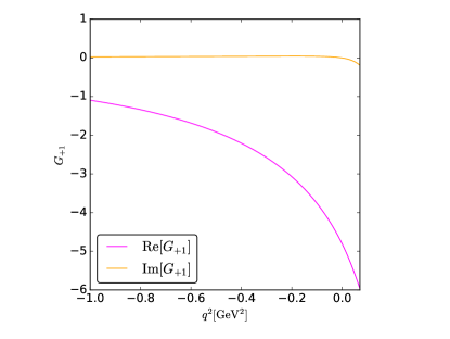
Figure 2: Real and imaginary part of $G_{+1}(q^{2})$.

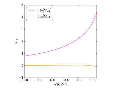
Figure 3: Real and imaginary part of $G_{-1}(q^{2})$.

We plot the single differential decay width $\mathrm{d}\Gamma/\mathrm{d}q^{2}$ for the Dalitz decay $\Sigma^{*}\rightarrow\Lambda e^{+}e^{-}$, i.e. the angular integral of (22), in the Dalitz region $4m_{e}^{2}<q^{2}<(m_{\Sigma^{*}}-m_{\Lambda})^{2}$. In particular in Fig. 4 we show a comparison with the corresponding QED case (24), for which the $q^{2}$-dependence of the TFFs is not resolved. The two curves show a slight off-set in the central region, but essentially coincide over the whole range. This implies that high resolution is needed from the experimental side in order to appreciate this discrepancy and gain new insight on the internal structure of hyperons.

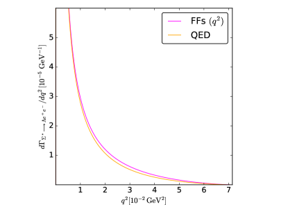
Figure 4: Single-differential decay width for the $\Sigma^{*}\rightarrow\Lambda e^{+}e^{-}$ Dalitz decay. The curve labeled “FFs$\,(q^{2})$” is the angular integral of (22). The other curve is the QED analogue, given by (24).

In the Dalitz region it is also meaningful to plot the three combinations of TFFs that appear in front of the trigonometric functions in the four-body decay expression (29), in order to compare their magnitude. Fig. 5 shows that one of them, the linear combination of $\lvert G_{+1}\rvert^{2}$ and $\lvert G_{-1}\rvert^{2}$ is dominant, making it very challenging to extract information on the individual TFFs. Yet with sufficient statistics and angular resolution for the four-body decay $\Sigma^{*}\to\Lambda\,e^{+}e^{-}\to p\pi^{-}\,e^{+}e^{-}$ one might get access to the smaller form factor combinations.

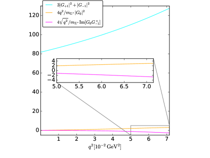
Figure 5: A comparison of the three combinations of TFFs in front of the trigonometric functions in (29) for the $\Sigma^{*}\rightarrow p\pi^{-}e^{+}e^{-}$ decay.

The situation might be compared to the history of the experimental determination of the pion-to-photon TFF and the corresponding radius from Dalitz decays $\pi^{0}\rightarrow\gamma e^{+}e^{-}$ as documented in the citations of Tanabashi et al. (2018). Also there one had to establish first the mere existence of the decay, then the approximate agreement with the QED case and finally with much higher experimental efforts the existence of a non-trivial form factor. We are looking forward to this future endeavor for the hyperon sector.

Appendix A Meson vs baryon dynamics

The purpose of this appendix is to discuss the different physical aspects that are contained in a dispersive determination of the low-energy TFFs. As an integral part of the main text it might distract the reader too much from the presentation of conceptual developments and results. Therefore we dedicate this appendix to this discussion.

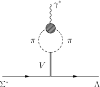
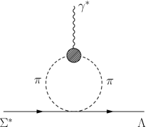
Figure 6: One-loop diagrams contained in our approach. The shaded blob denotes the pion vector form factor. The first diagram leads to the amplitude $K$ in (45).

To understand the physical content of our approach, it might be illuminating to study a form factor on the one-loop level. This is displayed in Fig. 6. Before discussing these diagrams, we stress that the dispersive approach contains more than these one-loop diagrams by including in (45) the complete rescattering of pions via their measured pion phase shift. The first diagram in Fig. 6 displays the exchange of a hyperon $Y$ in the crossed channels. The second diagram shows the formation of a vector meson $V$. The third diagram contains a contact interaction between the hyperons and the pions. A contact interaction is without structure. It contributes with a polynomial to the hyperon-pion scattering amplitude. Thus the contact interaction provides a contribution to the polynomial $P$ in (45). For the following discussion we call this contribution $P_{c}$.

Next we want to specify the relevant exchange hadrons $Y$ and $V$. If such a hadron is very heavy, its pole and cut structures caused by its propagator are not resolved. It contributes effectively like a contact interaction. Thus what is not covered (at the one-loop level) by the third diagram of Fig. 6 are exchanges of light hadrons. Concerning the baryon exchange diagrams, we have included explicitly the relevant lightest baryon states from the octet and decuplet. We call the impact of these processes on the form factors the “aspect of baryon dynamics”. Below we will show a calculation that focuses only on this aspect. The second and third diagram of Fig. 6 couple the external baryons directly to mesons. Therefore we call the impact of these processes on the form factors the “aspect of meson dynamics”. This part might be linked to the notion of vector meson dominance Sakurai (1969). Below we will also show a calculation that focuses only on this aspect.

Figure 7: Diagrammatic representation of all processes that do not contain the cross-channel exchange of light baryons. The shaded blob with four pion legs represents the S-matrix of pion scattering. The black dot contains the contact interaction of the third diagram of Fig. 6 and the strength mediated by the vector meson of the second diagram of Fig. 6. This black dot leads to the polynomial $P$ in (45).

Finally, let us look at the second diagram of Fig. 6 in more detail. The dynamics of the lightest vector meson, the $\rho$-meson, is automatically contained in the measured pion phase shift because the $\rho$-meson couples essentially with 100%  to a two-pion state. Diagrammatically the second and the third diagram of Fig. 6 are covered by the diagram of Fig. 7.

What is not automatically covered is the initial coupling strength with which the vector meson $V$ couples the pions to the hyperons. Schematically

$$ig_{BV}\,\bar{B}\gamma_{\mu}\gamma_{5}T_{\nu}V^{\mu\nu}+iG_{V}\,[u_{\mu},u_{\nu}]\,V^{\mu\nu}$$

$$\to\frac{g_{BV}\,G_{V}}{M_{V}^{2}}\,\bar{B}\gamma_{\mu}\gamma_{5}T_{\nu}\,[u^{\mu},u^{\nu}]\,,$$ (115)

which leads to

$$P=P_{c}+P_{V}\quad\mbox{with}\quad P_{V}\sim\frac{g_{BV}\,G_{V}}{M_{V}^{2}}\,.$$ (116)

In Appendix D and in Ecker et al. (1989a), respectively, the flavor structure of (115) is specified, which is, however, of no concern for our qualitative discussion. We will show below in more detail how the dynamics contained in the second diagram of Fig. 6 emerges from the dispersive framework by translating and simplifying this framework to the vector meson dominance language.

The result of the present discussion is that our dispersive framework contains all processes of Fig. 6 if the contact interaction strength $\sim P$ of Fig. 7 is determined by a fit to experiment. Without further theory input, this needs to be done separately for each form factor. If we need to estimate the size of $P$ on the theory side, we must include the influence of vector mesons as shown in (116) and carried out in Appendix D. In this context, we note that a pion-hyperon contact term of a given order in $\chi$PT leads to a contribution of the same order for the form factor. To be concrete, the TFFs $F_{i}$ of (2) start at second, third and fourth chiral order for $i=1,2,3$, respectively. Correspondingly, to fully account for the contribution of the $\rho$-meson to the TFF $F_{i}$ requires a pion-hyperon contact interaction from the chiral Lagrangian of $(i+1)$th order. With our present NLO input, we have a full coverage of $F_{1}$ only. In turn, $F_{1}$ constitutes the leading contribution to the TFFs $G_{\pm 1}$ in (8), (10). In addition, our formalism contains the pertinent contributions to all TFFs from the baryon dynamics induced by the first diagram of Fig. 6.

Baryon form factors are influenced by meson dynamics and by baryon dynamics. Therefore it might be illuminating to disentangle the meson and the baryon dynamics by switching off one of the two aspects. This will be discussed in the following two subsections. Yet we would like to stress that both cases miss part of the physics.

A.1 Pure meson dynamics

To focus on the impact of pion rescattering, we switch off the aspect of baryon dynamics, i.e. we put $K\to 0$ for the calculation of the hyperon-pion scattering amplitude $T$ in (45). Consequently, we put $f\to 0$ in (53) and (60). For simplicity we use the unsubtracted dispersion relation (64). Since we want to focus on the low-energy aspects, we also leave out the effective-pole term, i.e. $c_{m}\to 0$. Thus we obtain finally

$$G_{\rm pure\,meson}(q^{2})=\frac{P}{12\pi}\,\int\limits_{4m_{\pi}^{2}}^{\infty}\frac{\text{d}s}{\pi}\,\frac{\Omega(s)\,p_{\rm c.m.}^{3}(s)\,F^{V*}_{\pi}(s)}{s^{1/2}\,(s-q^{2}-i\epsilon)}\,.$$ (117)

Since the subtraction constant = contact interaction strength $P$ is just a number that does not influence the $s$ dependence of the integrand, we have not specified the TFF by any label. We show its generic form in Fig. 8(a), in the unphysical region between the two-pion threshold and 1 GeV². Obviously, the TFF displays the influence of the $\rho$-meson, i.e. the mesonic aspects are very well covered. An unphysical aspect emerges from the fact that the imaginary part of the TFF vanishes below the two-pion threshold. In reality, the TFF is complex everywhere, since the $\Sigma^{*}$ is unstable. This is, however, hardly visible in the full results for $G_{-1}$ in Fig. 8(b), since the imaginary part at $q^{2}\approx 4m_{\pi}^{2}$ becomes extremely tiny. From the comparison of Figs. 8(a), 8(b), one sees that if one adjusted the $\rho$-peak of the imaginary parts to the same size, then the peak of the real part of the full calculation will be somewhat smaller than the one of the pure-meson calculation. Moreover at low energies the curvature in the real part of the full $G_{-1}$ is milder with respect to the pure-meson calculation.

A relation to strict vector meson dominance can be deduced from (117). Suppose that the width of the vector meson is small. Essentially this means that the pion phase shift is zero below the vector meson mass and $\pi$ above. This leads to $\Omega(s)=m_{\rho}^{2}/(m_{\rho}^{2}-s)$. With a slight refinement, $m_{\rho}^{2}-s\to m_{\rho}^{2}-s-im_{\rho}\Gamma_{\rho}$, one obtains $\Omega(s)\,F^{V*}_{\pi}(s)\sim\delta(s-m_{\rho}^{2})/\Gamma_{\rho}$ and therefore $G_{\rm pure\,meson}(q^{2})\sim P/\Gamma_{\rho}\cdot 1/(m_{\rho}^{2}-q^{2})$. The appearance of the ratio $P/\Gamma_{\rho}$ has a natural interpretation: In a vector meson dominance picture the contact term $\sim P$ for the hyperon-pion scattering amplitude emerges from integrating out the vector meson, see (115), (116). This leads to $P\sim g_{B\rho}\,G_{V}$. On the other hand, in strict vector meson dominance, the coupling of the vector meson to the pions must be adjusted such that the correct electric charge of the pion emerges that is independent of strong-interaction coupling constants, i.e. $G_{V}\sim 1/F_{V}$ where $F_{V}$ denotes the coupling strength with which the photon couples to the vector meson. Thus one finds $P/\Gamma_{\rho}\sim P/G_{V}^{2}\sim g_{B\rho}/G_{V}\sim g_{B\rho}F_{V}$. This is exactly what one expects as the coefficient of a form factor obtained in the vecor meson dominance framework, i.e. in full analogy to (115) one finds

$$ig_{BV}\,\bar{B}\gamma_{\mu}\gamma_{5}T_{\nu}V^{\mu\nu}+F_{V}\,f_{+}^{\mu\nu}\,V_{\mu\nu}$$

$$\to i\,\frac{g_{BV}\,F_{V}}{M_{V}^{2}}\,\bar{B}\gamma_{\mu}\gamma_{5}T_{\nu}\,f_{+}^{\mu\nu}\,.$$ (118)

m

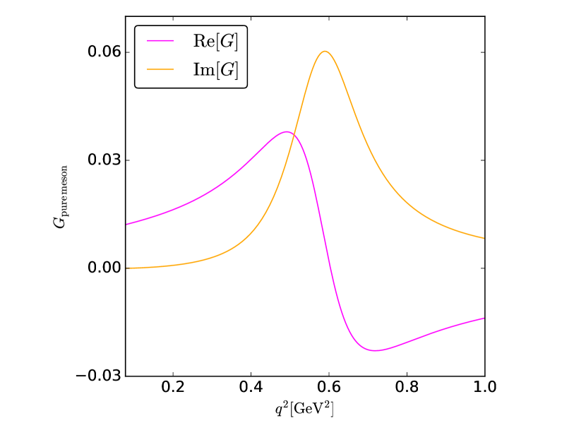
(a)

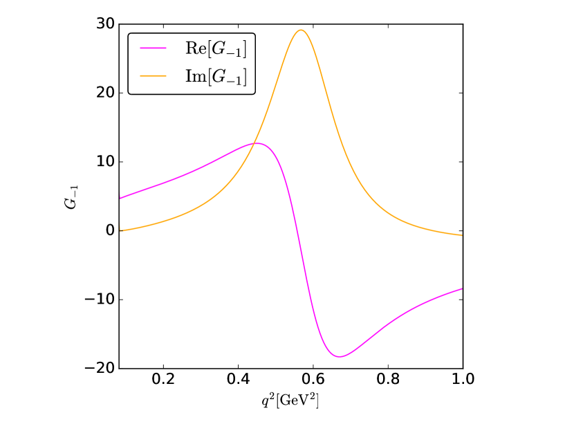
(b)

Figure 8: Pure mesonic contribution to the TFFs (a) in arbitrary units, compared with the full $G_{-1}(q^{2})$ described by meson and baryon dynamics together (b), in the unphysical timelike region $4m_{\pi}^{2}<q^{2}<1$ GeV².

Thus the dispersive framework reproduces and refines the vector meson dominance aspects. The only input one needs is the initial strength (contact interaction) with which the pions couple to the baryons. In the vector meson dominance setup this is obtained by integrating out the vector meson. One can also rephrase it in the following way: If one integrates out the vector meson for the interaction terms between the vector meson and the baryons and between the vector meson and the photon, one obtains a photon-baryon coupling right away. The dispersive framework produces the same with the pions as intermediate agents. Of course, the dispersive framework based on data for the pion phase shift and the pion vector form factor is more acurate than the schematic and model-dependent vector meson dominance scenario but it covers qualitatively the same physics. In addition, the dispersive framework presented in this paper contains also the aspects of baryon dynamics that is completely missing in the vector meson dominance approach.

A.2 Pure baryon dynamics

To focus on the impact of the processes where baryons are exchanged in the cross channel, we switch off the contact interaction and the pion rescattering. For simplicity we use an unsubtracted dispersion relation. Thus we put $F_{\pi}^{V}\to 1$ in (64) and (60). Since we want to focus on the low-energy aspects, we also leave out the effective-pole term, i.e. $c_{m}\to 0$. For the calculation of the scattering amplitude $T$ we put $P\to 0$ and $\delta\to 0$ in (45). This also implies that the anomalous piece vanishes. In simple terms: $T_{m}\to K_{m}$ in (64). This leads to

$$G^{\rm pure\,baryon}_{m}(q^{2}) = \frac{1}{12\pi}\,\int\limits_{4m_{\pi}^{2}}^{\Lambda^{2}}\frac{\text{d}s}{\pi}\,\frac{K_{m}(s)\,p_{\rm c.m.}^{3}(s)}{s^{1/2}\,(s-q^{2}-i\epsilon)}$$ (119)

$${}+\frac{1}{12\pi}\,\int\limits_{0}^{1}\text{d}x\,\frac{ds^{\prime}(x)}{dx}\,\frac{1}{s^{\prime}(x)-q^{2}}$$

$$\times\frac{f_{m}(s^{\prime}(x))\,s^{\prime}(x)}{-4\,(-\lambda(s^{\prime}(x),m_{\Sigma^{*}}^{2},m_{\Lambda}^{2}))^{3/2}}\,.\phantom{mm}$$

In Fig. 9(a) this contribution is plotted for the TFF $G_{-1}(q^{2})$, in the range $-1<q^{2}\,[\mathrm{GeV}^{2}]<1$. As expected the form factor has an imaginary part for all values of $q^{2}$, even if very tiny for $q^{2}<0$. The baryon exchange diagrams contain the physical aspect that the $\Sigma^{*}$ is unstable. What is missing, of course, is the influence of the $\rho$-meson, i.e. the mesonic aspects. For comparison we show in Fig. 9(b) also the complete result for $G_{-1}(q^{2})$, taking into account the contributions of both meson and baryon dynamics, again across the space- and timelike regions. Note that the same quantity has been previously plotted (Fig. 8(b)) but in a different range. This time we include the negative $q^{2}$ physical region and focus on the region around $q^{2}=0$. There we notice in Fig. 9a a steep rise in the real part, which is mitigated in Fig. 9b by the $\rho$-meson tail. In summary, even if the $\rho$-meson dictates in general the shape and size of the form factor, the low-energy behavior is significantly influenced by the baryon dynamics. m

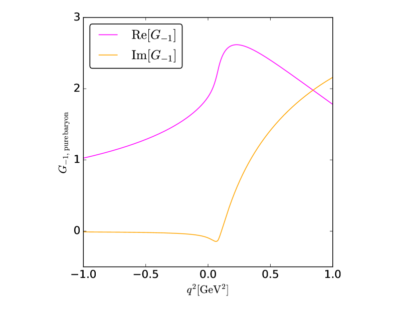
(a)

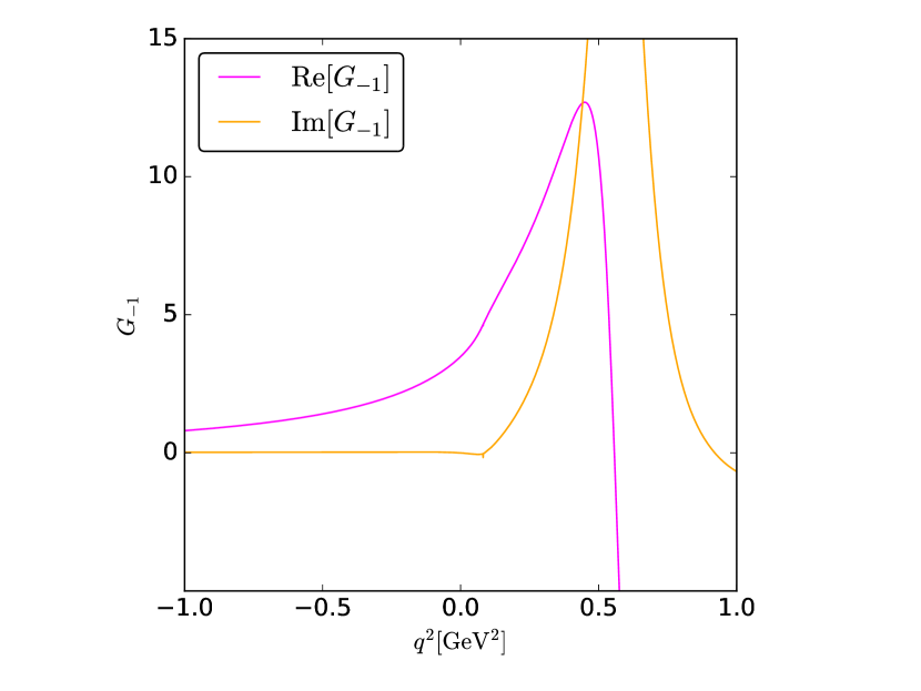
(b)

Figure 9: Pure baryonic contribution to $G_{-1}(q^{2})$ (a) as compared to the full result for $G_{-1}(q^{2})$ described by meson and baryon dynamics together (b), in the range $-1<q^{2}\,[\mathrm{GeV}^{2}]<1$.

Appendix B Projector formalism for helicity amplitudes

Spin-3/2 objects can be obtained from the coupling of spin-1/2 and spin-1 states. Thus we construct a spin-3/2 vector-spinor Rarita and Schwinger (1941) by

$$u^{\mu}(p,\sigma)=\sum\limits_{\rho,\lambda}\left(\frac{3}{2},\sigma\right|1,\rho\,;\left.\frac{1}{2},\lambda\right)\,u(p,\lambda)\,\varepsilon^{\mu}(p,\rho)\phantom{mm}$$ (120)

with a spin-1/2 spinor $u$, a spin-1 polarization vector $\varepsilon^{\mu}$ and a Clebsch-Gordan coefficient $(J,M|j_{1},m_{1};j_{2},m_{2})$. Here in slight contrast to the rest of this work the spin projections on a given quantization axis (and not the helicities) are denoted by $\sigma$, $\lambda$ and $\rho$, respectively. Yet if one chooses the quantization axis along the flight direction (as we will do in a moment) then helicity and spin projection coincide.

It is useful to provide (120) in an explicit form:

$$u^{\mu}(p,\pm 3/2) = u(p,\pm 1/2)\,\varepsilon^{\mu}(p,\pm 1)\,,$$

$$u^{\mu}(p,\pm 1/2) = \frac{1}{\sqrt{3}}\,u(p,\mp 1/2)\,\varepsilon^{\mu}(p,\pm 1)$$ (121)

$${}+\frac{\sqrt{2}}{\sqrt{3}}\,u(p,\pm 1/2)\,\varepsilon^{\mu}(p,0)\,.$$

For the spin-1/2 spinors we use the conventions of Peskin and Schroeder (1995). For the spin-1 polarization vectors for massive states we provide here only their explicit form for the case where the $z$-direction constitutes both the spin quantization axis and the direction of motion of the particle Penner (1999); Stoica et al. (2011):

$$\varepsilon^{\mu}(p_{z},\pm 1)=\frac{\mp 1}{\sqrt{2}}\,(0,1,\pm i,0)\,,$$

$$\varepsilon^{\mu}(p_{z},0)=(p_{z}/m,0,0,E/m)$$ (122)

where $m$ denotes the mass of the particle and $E$ its energy. Note that the coefficient $\mp 1$ does not show up in the definitions of Peskin and Schroeder (1995).

Irrespective of flight direction and spin quantization axis the spin-3/2 vector-spinors satisfy

$$\sum\limits_{\sigma}u_{\mu}(p,\sigma)\,\bar{u}_{\nu}(p,\sigma)=-(\not{p}+m)\,P^{3/2}_{\mu\nu}(p)$$ (123)

where $p^{0}=\sqrt{m^{2}+\vec{p}^{2}}$ denotes the energy of the particle described by the vector-spinor and $m$ its mass. The projector on spin 3/2 is defined by

$$P^{3/2}_{\mu\nu}(p):=g_{\mu\nu}-\frac{1}{3}\,\gamma_{\mu}\gamma_{\nu}-\frac{1}{3p^{2}}\,(\not{p}\,\gamma_{\mu}\,p_{\nu}+p_{\mu}\,\gamma_{\nu}\,\not{p})\,.\phantom{mm}$$ (124)

Note that for (123) the scalar product $p^{2}$ appearing in (124) can be replaced by $m^{2}$.

For our Lagrangian (67) a spin-3/2 (vector-spinor) field $\psi_{\mu}(x)$ has the following propagator de Jong and Malfliet (1992); Hacker et al. (2005)

$$\langle 0|{\rm T}\psi_{\mu}(x)\,\bar{\psi}_{\nu}(y)|0\rangle=\int\frac{\text{d}^{4}p}{(2\pi)^{4}}\,i\,S_{\mu\nu}(p)\,e^{-ip(x-y)}\phantom{mm}$$ (125)

with

$$S_{\mu\nu}(p) := -\frac{\not{p}+m}{p^{2}-m^{2}+i\epsilon}\,P^{3/2}_{\mu\nu}(p)+\frac{2}{3m^{2}}\,(\not{p}+m)\,\frac{p_{\mu}p_{\nu}}{p^{2}}$$ (126)

$${}-\frac{1}{3m}\,\frac{p_{\mu}\,p^{\alpha}\,\gamma_{\alpha\nu}+\gamma_{\mu\alpha}\,p^{\alpha}\,p_{\nu}}{p^{2}}\,.$$

Note that for the propagator of (125), (126) the scalar product $p^{2}$ appearing in (124) cannot be replaced by $m^{2}$. The propagator (126) describes propaging modes of spin 3/2 and frozen modes of spin 1/2 de Jong and Malfliet (1992).

The scattering amplitudes for the reaction $\Sigma^{*}\,\bar{\Lambda}\to\pi^{+}\pi^{-}$ have the following structure:

$$\bar{v}_{\Lambda}(p_{\Lambda},\lambda)\,M_{\mu}(p_{\Sigma^{*}},p_{\Lambda},k)\,u^{\mu}_{\Sigma^{*}}(p_{\Sigma^{*}},\sigma)$$ (127)

with $k:=p_{\pi^{+}}-p_{\pi^{-}}$. Feynman rules can provide a quite lengthy expression for the spinor $4\times 4$ matrix $M^{\mu}$. Therefore we aim at a projector formalism where (127) is related to scalar quantities $a_{i}$ and a pre-defined set of spinor objects such that only the scalar quantities depend on the explicit form of $M^{\mu}$, i.e.

$$\bar{v}_{\Lambda}\,M_{\mu}\,u^{\mu}_{\Sigma^{*}}=\sum\limits_{i}a_{i}\;\bar{v}_{\Lambda}\,M_{i}^{\mu}\,g_{\mu\nu}\,u^{\nu}_{\Sigma^{*}}\,.$$ (128)

The tasks are to construct a complete set of linearly independent structures $M_{i}^{\mu}$ and to find a convenient way to determine $a_{i}$ from an arbitrary $M^{\mu}$. Such an endeavor is similar in spirit to Stoica et al. (2011).

Due to parity symmetry we can focus on the case where the $\bar{\Lambda}$ has positive helicity, $\lambda=+1/2$. Then we need four pre-defined spinor objects corresponding to the possible values for the helicity of the $\Sigma^{+}$ baryon, $\sigma=+3/2,+1/2,-1/2,-3/2$. It is convenient to introduce the following four-vectors:

$$q:=p_{\Sigma^{*}}+p_{\Lambda}\,,\qquad\bar{k}:=p_{\Sigma^{*}}-p_{\Lambda}\,,$$

$$r:=\bar{k}-\frac{\bar{k}\cdot q}{q^{2}}\,q\,,\qquad k_{\perp}:=k-\frac{k\cdot r}{r^{2}}\,r\,.$$ (129)

In the center-of-mass frame with the three-momentum of the $\Sigma^{*}$ pointing in the $z$-direction and the reaction taking place in the $x$-$z$ plane one finds that $q$ has only a zeroth component, $r$ has only a third ($z$) component and $k_{\perp}$ has only a first ($x$) component.

We are looking now for four independent structures of type $M^{\mu}$ in (127). In general, $M^{\mu}$ contains products of $\gamma$ matrices and exactly one $\gamma_{5}$. All $\gamma$ matrices that are contracted with $p_{\Lambda}$, $p_{\Sigma^{*}}$ or the spin-3/2 spinor $u_{\Sigma^{*}}$ can be moved towards $\bar{v}_{\Lambda}$ or $u_{\Sigma^{*}}$ and eliminated by equations of motion. This results in structures with less many $\gamma$ matrices. If two $\gamma$ matrices are contracted with each other or with the very same four-momentum, then one can also simplify the expression.

This whole procedure leaves us with four independent structures of $M^{\mu}$ type:

$$\gamma_{5}\,k_{\perp}^{\mu}\,,\quad\gamma_{5}\,p^{\mu}_{\Lambda}\,,\quad\not{k}_{\perp}\gamma_{5}\,p^{\mu}_{\Lambda}\,,\quad\not{k}_{\perp}\gamma_{5}\,k^{\mu}_{\perp}\,.$$ (130)

It is simpler, however, to use the following linear combinations:

$$M^{\mu}_{1} := \left(q^{2}-(m_{\Sigma^{*}}+m_{\Lambda})^{2}\right)\gamma_{5}\,k_{\perp}^{\mu}-m_{\Sigma^{*}}\,\not{k}_{\perp}\gamma_{5}\,p^{\mu}_{\Lambda}\,,$$

$$M^{\mu}_{2} := \gamma_{5}\,p^{\mu}_{\Lambda}\,,$$

$$M^{\mu}_{3} := \not{k}_{\perp}\gamma_{5}\,p^{\mu}_{\Lambda}\,,$$

$$M^{\mu}_{4} := \left(q^{2}-(m_{\Sigma^{*}}-m_{\Lambda})^{2}\right)\not{k}_{\perp}\gamma_{5}\,k_{\perp}^{\mu}-m_{\Sigma^{*}}\,k_{\perp}^{2}\gamma_{5}\,p^{\mu}_{\Lambda}\,.$$

They are constructed such that in the center-of-mass frame they satisfy

$$\bar{v}_{\Lambda}(p_{\Lambda},+1/2)\,M^{\mu}_{i}\,g_{\mu\nu}\,u^{\nu}_{\Sigma^{*}}(p_{\Sigma^{*}},\sigma)\sim\delta_{i\,i_{\Sigma^{*}}}$$ (132)

with $i_{\Sigma^{*}}:=5/2-\sigma$. In other words, each $M_{i}^{\mu}$ contributes only to one helicity amplitude. Thus the sum in (128) reduces to only one term.

The remaining task is to find the scalar quantity $a_{i}$ for a given $M^{\mu}$. What makes the task non-trivial is the fact that different $M^{\mu}$ lead to the same $a_{i}$ because of the equations of motion for $\bar{v}_{\Lambda}$ and $u^{\nu}_{\Sigma^{*}}$. Therefore we construct on- and off-shell projectors to decompose a completely general $M^{\mu}$. Since $M^{\mu}$ is a $4\times 4$ spinor matrix with $\mu$ ranging from 0 to 3 we need in general a basis of 64 Lorentz-spinor structures. Due to parity symmetry we can restrict ourselves to 32 structures. For the first 4 terms we use

$$T_{\mu}^{i}:=P_{\rm on}^{\Lambda}\,M_{i}^{\nu}\,P_{\rm on}^{\Sigma^{*}}\,P^{3/2}_{\nu\mu}$$ (133)

introducing the projectors de Jong and Malfliet (1992)

$$P_{\rm on}^{\Lambda} := \frac{1}{2m_{\Lambda}}\,(m_{\Lambda}-\not{p}_{\Lambda})\,,\quad P_{\rm off}^{\Lambda}:=\frac{1}{2m_{\Lambda}}\,(m_{\Lambda}+\not{p}_{\Lambda})\,,\phantom{m}$$

$$P_{\rm on}^{\Sigma^{*}} := \frac{1}{2m_{\Sigma^{*}}}\,(m_{\Sigma^{*}}+\not{p}_{\Sigma^{*}})\,,$$

$$P_{\rm off}^{\Sigma^{*}} := \frac{1}{2m_{\Sigma^{*}}}\,(m_{\Sigma^{*}}-\not{p}_{\Sigma^{*}})\,,\phantom{m}$$

$$P^{1/2}_{\mu\nu} := \frac{1}{3}\,\gamma_{\mu}\gamma_{\nu}+\frac{1}{3p_{\Sigma^{*}}^{2}}\,(\not{p}_{\Sigma^{*}}\gamma_{\mu}\,g_{\nu\alpha}+g_{\mu\alpha}\,\gamma_{\nu}\,\not{p}_{\Sigma^{*}})\,p_{\Sigma^{*}}^{\alpha}\,,$$

$$P^{3/2}_{\mu\nu} := g_{\mu\nu}-P^{1/2}_{\mu\nu}\,.$$ (134)

The other 28 structures are obtained from (133) by exchanging $P_{\rm on}^{\Lambda}$ by $P_{\rm off}^{\Lambda}$ and/or $P_{\rm on}^{\Sigma^{*}}$ by $P_{\rm off}^{\Sigma^{*}}$ and/or $P^{3/2}_{\nu\mu}$ by $P^{1/2}_{\nu\mu}$. We do not specify how we enumerate these structures from $i=5$ to $i=32$ because we will not need them in the end. We also introduce the Dirac adjoint structures

$$\bar{T}_{\mu}^{i}:=\gamma_{0}\,(T_{\mu}^{i})^{\dagger}\,\gamma_{0}\,,\quad\mbox{for}\quad i=1,\ldots,32\,.$$ (135)

Provided that the $T_{\mu}^{i}$ form 32 linearly independent structures we can decompose any $M_{\mu}$ as

$$M_{\mu}=\sum\limits_{i=1}^{32}a_{i}\,T_{\mu}^{i}$$ (136)

with

$$a_{i}=\sum\limits_{j=1}^{32}(C^{-1})_{ij}\,{\rm Tr}(\bar{T}_{\mu}^{j}M^{\mu})$$ (137)

and the $32\times 32$ matrix $C$ with elements

$$C_{ij}:={\rm Tr}(\bar{T}_{\mu}^{i}\,T_{\nu}^{j})\,g^{\mu\nu}\,.$$ (138)

Here Tr denotes the spinor trace. We have checked explicitly that det$C\neq 0$ which shows that the 32 structures $T^{i}_{\mu}$ are linearly independent, i.e. form a basis to construct the most general $M_{\mu}$.

Inserting (136) in (127) and using the equations of motion for the spinors shows

$$\bar{v}_{\Lambda}\,M_{\mu}\,u^{\mu}_{\Sigma^{*}}=\sum\limits_{i=1}^{4}a_{i}\;\bar{v}_{\Lambda}\,M_{i}^{\mu}\,g_{\mu\nu}\,u^{\nu}_{\Sigma^{*}}\,.$$ (139)

Thus we only need to determine the four scalar quantities $a_{i}$ with $i=1,2,3,4$ from (137). Since the projectors in (B) are pairwise orthogonal one finds

$${\rm Tr}(\bar{T}_{\mu}^{i}T_{\nu}^{j})\,g^{\mu\nu}=0\quad\mbox{for}\quad i>4,\;j=1,2,3,4\,.$$ (140)

In addition, we have checked by an explicit calculation

$$C_{ij}\sim\delta_{ij}\quad\mbox{for}\quad i,j=1,2,3,4\,.$$ (141)

A result that one could have anticipated already from (132). Finally (137) simplifies to

$$a_{i}=\frac{{\rm Tr}(\bar{T}_{\mu}^{i}M^{\mu})}{C_{i}}$$ (142)

with

$$C_{i}:={\rm Tr}(\bar{T}_{\mu}^{i}\,T_{\nu}^{i})\,g^{\mu\nu}\,.$$ (143)

Explicit expressions are given by

$$C_{1} := \frac{k_{\perp}^{2}}{4\,m_{\Sigma^{*}}\,m_{\Lambda}}\,\left((m_{\Sigma^{*}}+m_{\Lambda})^{2}-q^{2}\right)\,\lambda(q^{2},m^{2}_{\Sigma^{*}},m^{2}_{\Lambda})\,,$$

$$C_{2} := \frac{-1}{12\,m^{3}_{\Sigma^{*}}\,m_{\Lambda}}\,\left((m_{\Sigma^{*}}-m_{\Lambda})^{2}-q^{2}\right)\,\lambda(q^{2},m^{2}_{\Sigma^{*}},m^{2}_{\Lambda})\,,$$

$$C_{3} := \frac{k_{\perp}^{2}}{12\,m^{3}_{\Sigma^{*}}\,m_{\Lambda}}\,\left((m_{\Sigma^{*}}+m_{\Lambda})^{2}-q^{2}\right)\,\lambda(q^{2},m^{2}_{\Sigma^{*}},m^{2}_{\Lambda})\,,$$

$$C_{4} := \frac{-(k_{\perp}^{2})^{2}}{4\,m_{\Sigma^{*}}\,m_{\Lambda}}\,\left((m_{\Sigma^{*}}-m_{\Lambda})^{2}-q^{2}\right)\,\lambda(q^{2},m^{2}_{\Sigma^{*}},m^{2}_{\Lambda})$$

with the Källén function defined in (12). In the center-of-mass frame one finds

$$k_{\perp}^{2}=-4\,p_{\rm c.m.}^{2}\,\sin^{2}\theta$$ (145)

with the center-of-mass momentum of the pions $p_{\rm c.m.}:=\sqrt{q^{2}-4m_{\pi}^{2}}/2$ and $\theta$ denoting the angle between the three-momenta of $\Sigma^{*}$ and $\pi^{+}$.

To summarize, for a given amplitude structure $M_{\mu}$ and a given helicity $\sigma$ we find in the center-of-mass frame

$$\bar{v}_{\Lambda}(p_{\Lambda},+1/2)\,M_{\mu}\,u^{\mu}_{\Sigma^{*}}(p_{\Sigma^{*}},\sigma)$$

$$=\frac{{\rm Tr}(\bar{T}_{\alpha}^{i}M^{\alpha})}{C_{i}}\;\bar{v}_{\Lambda}(p_{\Lambda},+1/2)\,M_{i}^{\mu}\,g_{\mu\nu}\,u^{\nu}_{\Sigma^{*}}(p_{\Sigma^{*}},\sigma)\phantom{mm}$$ (146)

with $i=5/2-\sigma$. Note in particular that in (146) there is no implicit summation over $i$, it is fixed by the choice of $\sigma$, the helicity of the $\Sigma^{*}$.

In the main text we have introduced reduced amplitudes (44) for the dispersive representation of the TFFs. To make contact with these reduced amplitudes we present here the ratios

$$\frac{\bar{v}_{\Lambda}(-p_{z},+1/2)\,M_{1}^{\mu}\,g_{\mu\nu}\,u^{\nu}_{\Sigma^{*}}(p_{z},+3/2)}{\bar{v}_{\Lambda}(-p_{z},+1/2)\,\gamma_{5}\,u^{1}_{\Sigma^{*}}(p_{z},+3/2)\,p_{\rm c.m.}}$$

$$=-2\,\sin\theta\left(q^{2}-(m_{\Sigma^{*}}+m_{\Lambda})^{2}\right)\,,$$

$$\frac{\bar{v}_{\Lambda}(-p_{z},+1/2)\,M_{2}^{\mu}\,g_{\mu\nu}\,u^{\nu}_{\Sigma^{*}}(p_{z},+1/2)}{\bar{v}_{\Lambda}(-p_{z},+1/2)\,\gamma_{5}\,u^{3}_{\Sigma^{*}}(p_{z},+1/2)\,p_{\rm c.m.}}$$

$$=\frac{2\,q^{2}}{m_{\Sigma^{*}}^{2}-m_{\Lambda}^{2}+q^{2}}\,\frac{p_{z}}{p_{\rm c.m.}}\,,$$

$$\frac{\bar{v}_{\Lambda}(-p_{z},+1/2)\,M_{3}^{\mu}\,g_{\mu\nu}\,u^{\nu}_{\Sigma^{*}}(p_{z},-1/2)}{\bar{v}_{\Lambda}(-p_{z},+1/2)\,\gamma_{5}\,u^{1}_{\Sigma^{*}}(p_{z},-1/2)\,p_{\rm c.m.}}$$

$$=-2\,\sin\theta\;\frac{q^{2}-(m_{\Sigma^{*}}+m_{\Lambda})^{2}}{m_{\Sigma^{*}}}$$ (147)

with $p_{z}:=\lambda^{1/2}(q^{2},m^{2}_{\Sigma^{*}},m^{2}_{\Lambda})/(2\sqrt{q^{2}})$ denoting the center-of-mass momentum of $\Sigma^{*}$ and $\bar{\Lambda}$. Note that for the $M_{2}$ case (non-flip amplitude) there will always be a factor $p_{z}\,p_{\rm c.m.}$ from the partial-wave projection of ${\rm Tr}(\bar{T}_{\alpha}^{2}M^{\alpha})$. Together with the last ratio on the right-hand side of the corresponding equation in (147) this leads to an expression for the reduced amplitude without any square roots.

In practice the whole task of dealing with a Feynman scattering amplitude for given helicities is reduced to the calculation of one spinor trace ${\rm Tr}(\bar{T}_{\alpha}^{i}M^{\alpha})$.

Appendix C Dispersive representations, cuts and anomalous thresholds

This appendix has two purposes. First, we provide a detailed discussion of the analytic structure of a scalar triangle diagram. This resembles the first diagram shown in Fig. 6, except that one deals with p-waves there and with s-waves in the scalar case. But the appearance of anomalous thresholds has the very same pattern. Therefore we use the scalar triangle as a test case to check that we include all bits and pieces in the correct way for our TFF calculations. The second purpose is the derivation of (53), (60), and (63).

Consider the result of a triangle loop diagram Karplus et al. (1958); ’t Hooft and Veltman (1979); Lucha et al. (2007); Hoferichter et al. (2014),

$$C(s) = \frac{1}{i\pi^{2}}\int\!\text{d}^{4}l\,\frac{1}{(l^{2}-m_{\rm exch}^{2})\left((l+p_{1})^{2}-m_{\pi}^{2}\right)\left((l-p_{2})^{2}-m_{\pi}^{2}\right)}\,,$$ (148)

which can be calculated directly when rewritten as

$$C(s) = \int\limits_{0}^{1}\!\text{d}x_{1}\,dx_{2}\,dx_{3}\,\delta(1-x_{1}-x_{2}-x_{3})\left[x_{1}x_{3}m_{1}^{2}+x_{2}x_{3}m_{2}^{2}+x_{1}x_{2}s-x_{1}m_{\pi}^{2}-x_{2}m_{\pi}^{2}-x_{3}m_{\rm exch}^{2}\right]^{-1}$$ (149)

with $s:=(p_{1}+p_{2})^{2}$, $m_{1}^{2}:=p_{1}^{2}$ and $m_{2}^{2}:=p_{2}^{2}$. We consider first the case that $m_{\rm exch}^{2}$ is large enough and $m_{1}^{2}$ and $m_{2}^{2}$ are small enough. A quantitative specification will follow later. In this case, the imaginary part of $C$ (for real values of $s$) is just given by cutting Cutkosky (1960) the two pion lines of the Feynman diagram. The result is

$${\rm Im}C(s)=-\pi\,\frac{\sigma(s)}{\kappa(s)}\,\log\frac{Y(s)+\kappa(s)}{Y(s)-\kappa(s)}\,\Theta(s-4m_{\pi}^{2})$$ (150)

where

$$Y(s):=s+2m_{\rm exch}^{2}-m_{1}^{2}-m_{2}^{2}-2m_{\pi}^{2}\,,$$ (151)

$$\kappa(s):=\lambda^{1/2}(s,m_{1}^{2},m_{2}^{2})\,\sigma(s)\,,$$ (152)

and

$$\sigma(s):=\sqrt{1-\frac{4m_{\pi}^{2}}{s}}\,.$$ (153)

We use the log and the square root function both with a cut on the real negative axis.

The triangle function $C$ can be represented by a dispersive integral in the variable $s$ ranging from the two-pion threshold to infinity (unitarity cut):

$$C(z)=\int\limits_{4m_{\pi}^{2}}^{\infty}\frac{ds^{\prime}}{\pi}\frac{{\rm Im}C(s^{\prime})}{s^{\prime}-z}=\int\limits_{4m_{\pi}^{2}}^{\infty}\frac{ds^{\prime}}{\pi}\frac{\sigma(s^{\prime})\,l(s^{\prime})}{s^{\prime}-z}$$ (154)

with

$$l(s):=-\frac{\pi}{\kappa(s)}\,\log\frac{Y(s)+\kappa(s)}{Y(s)-\kappa(s)}\,.$$ (155)

Here $z$ is an arbitrary complex number that does not lie on the unitarity cut, i.e. $z\not\in[4m_{\pi}^{2},+\infty[$.

It should be possible to find a dispersive representation of the function $C$ for any values of the masses. But it is necessary to study the cut structure of the logarithm in (155). If this cut intersects with the unitarity cut, one needs a proper analytic continuation of the logarithm along the unitarity cut and one picks up an anomalous contribution.

To understand these statements, we consider first the case where (154) works. In this case, $l(s)$ from (155) is a smooth function along and in the vicinity of the unitarity cut. Concerning the function $\sigma(s)$, it has a cut for $s\in[0,4m_{\pi}^{2}]$. It is convenient to define a function that has a cut along the unitarity cut Moussallam (2011):

$$\hat{\sigma}(z):=\sqrt{\frac{4m_{\pi}^{2}}{z}-1}\,.$$ (156)

For $s\in[4m_{\pi}^{2},+\infty[$ it satisfies

$$\hat{\sigma}(s\pm i\epsilon)=\mp i\sigma(s)\,.$$ (157)

By construction, the function $C(z)$ is defined via (154) in the whole complex plane except for the unitarity cut. This cut defines a second Riemann sheet. We construct a function $C^{\rm II}(z)$ that constitutes an analytic continuation of $C$ through the cut. For $s\in[4m_{\pi}^{2},+\infty[$ we demand

$$C^{\rm II}(s+i\epsilon) \stackrel{{\scriptstyle!}}{{=}} C(s-i\epsilon)=C(s+i\epsilon)-2i\sigma(s)\,l(s)$$ (158)

$$= C(s+i\epsilon)+2\hat{\sigma}(s+i\epsilon)\,l(s+i\epsilon)\,.$$

In the last step we have used (157) and the assumption that $l$ is a smooth function around the unitarity cut. This assumption will be critically reviewed below.

For the case at hand, we can use (158) to define an analytic continuation of $C$ on the second Riemann sheet:

$$C^{\rm II}(z):=C(z)+2\hat{\sigma}(z)\,l(z)\,.$$ (159)

The cut structure of $C^{\rm II}$ originates from the unitarity cut, from the additional cut of $\hat{\sigma}$ along the negative real axis and from the cut of the logarithm in the expression (155) for the function $l$. We note that the square root functions that define $\kappa$ in (152) and therefore enter (155) do not cause an additional cut because $l$ is an even function in $\kappa$.

Let us first focus on the unitarity cut. For $s\in[4m_{\pi}^{2},+\infty[$, we find

$$C^{\rm II}(s-i\epsilon) = C(s-i\epsilon)+2\hat{\sigma}(s-i\epsilon)\,l(s)$$ (160)

$$= C(s+i\epsilon)\,.$$

Thus the unitarity cut connects just the two Riemann sheets.

Next we focus on the log function. The branch points of the logarithm in (155) are given by $Y^{2}(s)=\kappa^{2}(s)$. They are located at

$$s_{\pm} = -\frac{1}{2}\,m_{\rm exch}^{2}+\frac{1}{2}\left(m_{1}^{2}+m_{2}^{2}+2m_{\pi}^{2}\right)$$ (161)

$${}-\frac{m_{1}^{2}\,m_{2}^{2}-m_{\pi}^{2}\,(m_{1}^{2}+m_{2}^{2})+m_{\pi}^{4}}{2m_{\rm exch}^{2}}$$

$${}\mp\frac{\lambda^{1/2}(m_{1}^{2},m_{\rm exch}^{2},m_{\pi}^{2})\,\lambda^{1/2}(m_{2}^{2},m_{\rm exch}^{2},m_{\pi}^{2})}{2m_{\rm exch}^{2}}$$

$$= \frac{1}{4m_{\rm exch}^{2}}\Big{[}(m_{1}^{2}-m_{2}^{2})^{2}$$

$$\phantom{mmmm}{}-\Big{(}\lambda^{1/2}(m_{1}^{2},m_{\rm exch}^{2},m_{\pi}^{2})$$

$$\phantom{mmmmmm}{}\pm\lambda^{1/2}(m_{2}^{2},m_{\rm exch}^{2},m_{\pi}^{2})\Big{)}^{2}\Big{]}\,.$$

The problem is that as a function of the masses, the values of $s_{\pm}$ move through the complex plane that constitutes the second Riemann sheet. If any of the two branch points hits the unitarity cut then this branch point moves on the physical (=first) Riemann sheet. To be specific, we take $s_{+}$ as the solution that has a positive imaginary part for small values of $m_{1}^{2}$. If one replaces $m_{1}^{2}$ by $m_{1}^{2}+i\epsilon$ and follows the motion of $s_{+}$ for increasing values of $m_{1}^{2}$, then $s_{+}$ moves towards the real axis and could intersect with the unitarity cut. Fig. 10 shows the trajectory of $s_{+}$ in the complex plane obtained by varying $m_{1}^{2}$, having fixed $m_{\mathrm{exch}}^{2}=m_{\Sigma}^{2}$ and $m_{2}^{2}=m_{\Lambda}^{2}$. Note the intersection with the unitarity cut, which implies that an additional cut must be located on the first Riemann sheet. The red dot indicates the actual position of $s_{+}$ for the physical choice $m_{1}^{2}=m_{\Sigma^{*}}^{2}$.

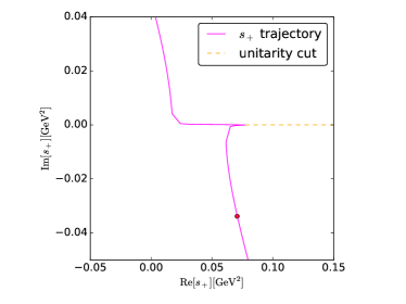
Figure 10: Real and imaginary part of $s_{+}$ obtained by varying $m_{1}^{2}$. The red dot corresponds to $m_{1}^{2}=m_{\Sigma^{*}}^{2}$, which is our case of interest.

Indeed, for

$$m_{1}^{2}+m_{2}^{2}-2m_{\pi}^{2}-2m_{\rm exch}^{2}=0\quad\mbox{(cross point)}$$ (162)

the two Källén functions in (161) become identical and one finds at this point

$$\left.s_{+}\right|_{\rm cross\,point}=4m_{\pi}^{2}\,,\quad\left.\frac{\partial s_{+}}{\partial m_{1}^{2}}\right|_{\rm cross\,point}=0\,,$$

$$\left.\frac{\partial^{2}s_{+}}{\partial(m_{1}^{2})^{2}}\right|_{\rm cross\,point}=\frac{2m_{\pi}^{2}}{\lambda(m_{2}^{2},m_{\rm exch}^{2},m_{\pi}^{2})}\,.\phantom{mm}$$ (163)

Therefore we obtain

$$\left.s_{+}(m_{1}^{2}+i\epsilon,\ldots)\right|_{\rm cross\,point}\approx$$

$$\left[s_{+}(m_{1}^{2},\ldots)+i\epsilon\,\frac{\partial s_{+}(m_{1}^{2},\ldots)}{\partial m_{1}^{2}}\right.$$

$$\left.{}-\frac{1}{2}\epsilon^{2}\,\frac{\partial^{2}s_{+}(m_{1}^{2},\ldots)}{\partial(m_{1}^{2})^{2}}\right]_{\rm cross\,point}$$

$$=4m_{\pi}^{2}-\epsilon^{2}\,\frac{m_{\pi}^{2}}{\lambda(m_{2}^{2},m_{\rm exch}^{2},m_{\pi}^{2})}\,.$$ (164)

In other words, the motion of $s_{+}$ just turns around (vanishing derivative) at the two-pion threshold. $s_{+}$ intersects with the unitarity cut if

$$\lambda(m_{2}^{2},m_{\rm exch}^{2},m_{\pi}^{2})<0\,.$$ (165)

One can already see in the original expression (155) that something goes wrong if $m_{1}^{2}$ becomes so large that (162) is satisfied. On the real axis, the log in (155) is ill-defined for $Y(s)=0$. From (151) we see that this zero of $Y$ is small as long as $m_{1}^{2}$ and $m_{2}^{2}$ are small and $m_{\rm exch}^{2}$ is large. But the zero of $Y$ reaches the unitarity cut, i.e. the branch point at the two-pion threshold for (162). For even larger values of $m_{1}^{2}$, i.e. for

$$m_{1}^{2}+m_{2}^{2}-2m_{\pi}^{2}-2m_{\rm exch}^{2}>0\,,$$ (166)

one needs a smooth analytic continuation of the logarithm along the unitarity cut. Otherwise, the dispersive representation (154) does not make sense. In addition, (154) is incomplete, because one has to circumvent also the branch point $s_{+}$, which is now on the physical Riemann sheet. It is convenient to choose the branch that starts at $s_{+}$ such that it intersects with the unitarity cut just at its own branch point at the two-pion threshold Hoferichter et al. (2014).

The two conditions for $s_{+}$ being located on the first Riemann sheet are (165) and (166). The dispersive representation of the triangle function (148) is then given by

$$C(s) = \frac{1}{2\pi i}\int\!\text{d}s^{\prime}\,\frac{{\rm disc}C(s^{\prime})}{s^{\prime}-s}$$ (167)

$$= \frac{1}{2\pi i}\int\limits_{4m_{\pi}^{2}}^{\infty}\!\text{d}s^{\prime}\,\frac{{\rm disc}_{\rm unit}C(s^{\prime})}{s^{\prime}-s}$$

$${}+\frac{1}{2\pi i}\int\limits_{0}^{1}\!\text{d}x\,\frac{\text{d}z(x)}{\text{d}x}\,\frac{{\rm disc}_{\rm anom}C(z(x))}{z(x)-s}\phantom{mm}$$

with the straight-line path connecting $s_{+}$ and the two-pion threshold,

$$z(x):=(1-x)s_{+}+x\,4m_{\pi}^{2}\,,$$ (168)

the function

$${\rm disc}_{\rm anom}C(z)=-\frac{4\pi^{2}i}{(-\lambda(z,m_{1}^{2},m_{2}^{2}))^{1/2}}\,,$$ (169)

and a piecewise defined function given by (cf. (150))

$$\frac{{\rm disc}_{\rm unit}C(s)}{2i}=$$ (170)

$$-\pi\,\frac{\sigma(s)}{\kappa(s)}\,\left[\log\frac{Y(s)+\kappa(s)}{Y(s)-\kappa(s)}+2\pi i\Theta\left((m_{1}-m_{2})^{2}-s\right)\right]$$

for $\lambda(s,m_{1}^{2},m_{2}^{2})>0$ while it is given by

$$\frac{{\rm disc}_{\rm unit}C(s)}{2i}=$$

$$-2\pi\frac{\sigma(s)}{\tilde{\kappa}(s)}\,\left[\arctan\frac{\tilde{\kappa}(s)}{Y(s)}+\pi\Theta(-Y(s))\right]$$ (171)

for $\lambda(s,m_{1}^{2},m_{2}^{2})<0$. This function is continuous along the unitarity cut except if $s=(m_{1}-m_{2})^{2}$ lies on the cut; there one has an integrable divergence. We have introduced

$$\tilde{\kappa}(s):=(-\lambda(s,m_{1}^{2},m_{2}^{2}))^{1/2}\,\sigma(s)\,.$$ (172)

In Fig. 11(a) the real and imaginary part of the triangle function (148) are plotted using $m_{1}=m_{\Sigma^{*}}$, $m_{\rm exch}=m_{\Sigma}$ and $m_{2}=m_{\Lambda}$. We have checked that the dispersive representation (167) for $s+i\epsilon$ with arbitrary real $s$ fully agrees with the direct calculation (149). We want to stress that ignoring the integration along the anomalous cut produces a very incomplete result, shown in Fig. 11(b).

Having established the correct analytic structure, we leave the case of the scalar triangle behind and turn to our TFFs, which have a different partial-wave structure and include the full pion rescattering.

m

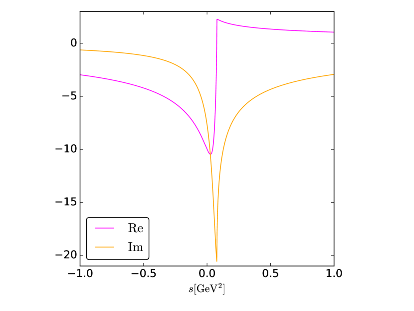
(a)

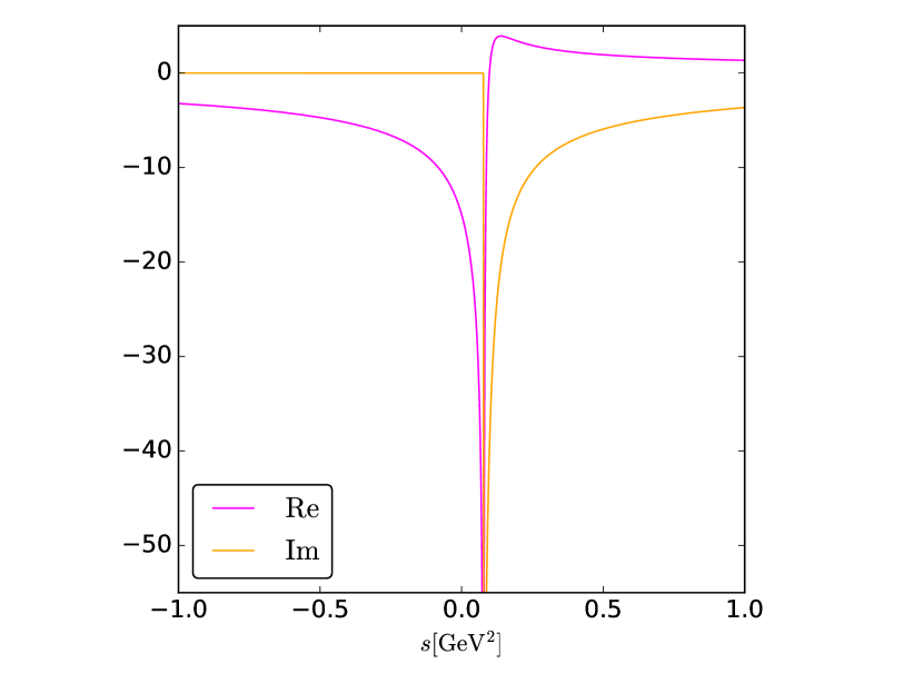
(b)

Figure 11: Comparison between (a) the triangle function (148), obtained by either (149) or (167), and (b) its incomplete dispersive representation (154), where only the unitarity cut has been taken into account, neglecting the presence of the anomalous cut. The masses involved here are $m_{1}=m_{\Sigma^{*}}$, $m_{\rm exch}=m_{\Sigma}$ and $m_{2}=m_{\Lambda}$.

For triangle diagrams with full two-pion rescattering we extend the usual formulae to allow for the presence of the anomalous cuts. We introduce the values of a function $A$ to the left ($A_{+}$) and to the right ($A_{-}$) of a (directed) cut line. The discontinuity of $A$ is then defined by

$${\rm disc}A:=A_{+}-A_{-}\,.$$ (173)

For a cut along the real axis this yields the well-known relations

$${\rm disc}A(s) = A(s+i\epsilon)-A(s-i\epsilon)$$ (174)

$$= A(s+i\epsilon)-A^{*}(s+i\epsilon)$$

$$= 2i{\rm Im}A(s+i\epsilon)\,.$$

The optical theorem that leads to (61) and (45) generalizes to

$${\rm disc}F=2i\frac{1}{24\pi}T_{+}\sigma p^{2}_{\rm cm}F_{\pi-}^{V}$$ (175)

and

$${\rm disc}(T-K)=2iT_{+}\sigma t_{-}$$ (176)

with the p-wave pion scattering amplitude $t$. Along the unitarity cut, the amplitude $t$ is given by $t=\sin\delta\,e^{i\delta}/\sigma$.

We recall how (176) is solved Omnes (1958). The Omnès function is introduced as a solution of

$${\rm disc}\Omega=2i\Omega_{+}\sigma t_{-}\,.$$ (177)

This allows to calculate

$${\rm disc}\frac{T-K}{\Omega} = \frac{(T-K)_{+}\Omega_{-}-(T-K)_{-}\Omega_{+}}{\Omega_{+}\Omega_{-}}$$ (178)

$$= \frac{(T-K)_{+}\Omega_{-}-(T-K)_{+}\Omega_{+}}{\Omega_{+}\Omega_{-}}$$

$${}+\frac{(T-K)_{+}\Omega_{+}-(T-K)_{-}\Omega_{+}}{\Omega_{+}\Omega_{-}}$$

$$= \frac{2iK_{+}\sigma t_{-}}{\Omega_{-}}\,.$$

The product $K\sigma$ is essentially proportional to the discontinuity of the triangle function $C$. The proportionality factor $h$ is a rational function of $s$, i.e. has no cuts. With the previous construction of disc$C$ we have achieved that the two cuts (unitarity cut and anomalous cut) do not intersect. Therefore we can write for the discontinuity (178) along the unitarity cut

$${\rm disc}\frac{T-K}{\Omega}=\frac{2iK\sigma t_{-}}{\Omega_{-}}=\frac{2iK\sin\delta}{|\Omega|}$$ (179)

because here $K$ is by construction a continuous function and $\Omega$ has the same phase as $t$. This leads to the standard dispersive part for $T-K$ explicitly given in (45). Along the anomalous cut we have

$${\rm disc}\frac{T-K}{\Omega}=2i\,h\,{\rm disc}_{\rm anom}C\,\frac{t_{-}}{\Omega_{-}}\,,$$ (180)

which leads to (53).

Finally we have to solve (175). For the unitarity cut we can just integrate the right-hand side of (175). For the anomalous cut we use (176) and find

$${\rm disc}_{\rm anom}F=\frac{1}{24\pi}\,{\rm disc}_{\rm anom}(T-K)\,p^{2}_{\rm cm}\,\frac{F_{\pi-}^{V}}{t_{-}}\,.$$ (181)

Since we have a dispersive representation for $T-K$ in (45), (53) we just need to read off the discontinuity along the anomalous cut. This leads to (63).

If one compares the expressions (53) and (63), one notices that (53) looks more complicated with $\Omega$ appearing outside and inside of the integral. Isn’t it possible to write (53) in a simpler way? After all, $\Omega$ is continuous along the anomalous cut. From (180) one sees that the discontinuity of $T-K$ along the anomalous cut is indeed just $2i\,h\,{\rm disc}_{\rm anom}C\,t$. The same can be obtained from (53). But the expression (53) inherits from $\Omega$ also a discontinuity along the unitarity cut. Therefore a direct dispersive representation of $T-K$ instead of the ratio $(T-K)/\Omega$ leads to an integral where in the integrand the integral of (53) appears. For the form factor we have this situation of a double integral anyway in (61) where the integral expressions for $T$ enter in the integrand. But for $T$ itself one can avoid the double integral representation if one lives with $\Omega$ appearing outside and inside of the integrals.

Appendix D Estimate for the NLO four-point pion-baryon coupling constant

Ideally the low-energy constant $c_{F}$ from (90) should be determined from experiment. To have a rough estimate for its size we apply a vector-meson-dominance (resonance-saturation) assumption Sakurai (1969); Ecker et al. (1989a, b); Meißner and Steininger (1997). To get a feeling for its accuracy we will make the same estimate for the octet sector. To this end, we consider the following part of the NLO Lagrangian of Holmberg and Leupold (2018):

$${\cal L}^{(2)}_{V} := i\,c_{M}\,({\cal O}_{\mu\nu})^{b}_{d}\,(f_{+}^{\mu\nu})^{d}_{b}+{\rm h.c.}$$ (182)

$${}+\frac{1}{4}\,c_{F}\,({\cal O}_{\mu\nu})^{b}_{d}\,([u^{\mu},u^{\nu}])^{d}_{b}+{\rm h.c.}$$

$${}+b_{M,D}\,{\rm tr}(\bar{B}\{f_{+}^{\mu\nu},\sigma_{\mu\nu}B\})$$

$${}+\frac{i}{2}\,b_{3,2}\,{\rm tr}(\bar{B}\{[u^{\mu},u^{\nu}],\sigma_{\mu\nu}B\})$$

with

$$({\cal O}_{\mu\nu})^{b}_{d}:=\epsilon_{ade}\,\bar{B}^{e}_{c}\,\gamma_{\mu}\gamma_{5}\,T_{\nu}^{abc}\,.$$ (183)

Estimates for $c_{M}$ and $b_{M,D}$ have been provided in Holmberg and Leupold (2018), based on fits to experimental data on radiative decays and magnetic moments, respectively: $|c_{M}|\approx 1.9\,$GeV^-1 and $b_{M,D}\approx 0.32\,$GeV^-1.

Vector-meson dominance Sakurai (1969) implies that the coupling strengths of hadrons to two pions (in a p-wave) and to photons are correlated. In the $\chi$PT framework this might be rephrased as the statement that the two building blocks $[u^{\mu},u^{\nu}]$ and $f_{+}^{\mu\nu}$ appear in a fixed combination, i.e. as the chiral field strength Ecker et al. (1989a, b)

$$\Gamma^{\mu\nu}:=\frac{1}{4}\,[u^{\mu},u^{\nu}]-\frac{i}{2}\,f_{+}^{\mu\nu}\,.$$ (184)

Under this assumption, we obtain the following estimates: $c_{F}\approx-2\,c_{M}$ and $b_{3,2}\approx b_{M,D}$. In Meißner and Steininger (1997), based on a resonance-saturation approach, the vector-meson contribution to the parameter $b_{3,2}$ (denoted by $b_{10}$ therein) has been estimated to $\approx$$\,0.5\,$GeV^-1, i.e. about 50% larger than our value for $b_{M,D}$. Therefore, we use as an estimate:

$$|c_{F}|=(4.8\pm 1.2)\,\mbox{GeV}^{-1}\quad\mbox{and}\quad\frac{c_{F}}{c_{M}}<0\,.$$ (185)

References

- Landsberg (1985) L. G. Landsberg, Phys. Rept. 128, 301 (1985).
- Czerwiński et al. (2012) E. Czerwiński, S. Eidelman, C. Hanhart, B. Kubis, A. Kupść, S. Leupold, P. Moskal, and S. Schadmand, eds., MesonNet Workshop on Meson Transition Form Factors (2012) arXiv:1207.6556 [hep-ph] .
- Miller (2007) G. A. Miller, Phys. Rev. Lett. 99, 112001 (2007), arXiv:0705.2409 [nucl-th] .
- Punjabi et al. (2015) V. Punjabi, C. F. Perdrisat, M. K. Jones, E. J. Brash, and C. E. Carlson, Eur. Phys. J. A51, 79 (2015), arXiv:1503.01452 [nucl-ex] .
- Körner and Kuroda (1977) J. G. Körner and M. Kuroda, Phys. Rev. D16, 2165 (1977).
- Carlson (1986) C. E. Carlson, Phys. Rev. D34, 2704 (1986).
- Pascalutsa et al. (2007) V. Pascalutsa, M. Vanderhaeghen, and S. N. Yang, Phys. Rept. 437, 125 (2007), arXiv:hep-ph/0609004 [hep-ph] .
- Kaxiras et al. (1985) E. Kaxiras, E. J. Moniz, and M. Soyeur, Phys. Rev. D32, 695 (1985).
- Kubis and Meißner (2001) B. Kubis and U.-G. Meißner, Eur. Phys. J. C18, 747 (2001), arXiv:hep-ph/0010283 [hep-ph] .
- Ablikim et al. (2019) M. Ablikim et al. (BESIII), Phys. Rev. Lett. 123, 122003 (2019), arXiv:1903.09421 [hep-ex] .
- Granados et al. (2017) C. Granados, S. Leupold, and E. Perotti, Eur. Phys. J. A53, 117 (2017), arXiv:1701.09130 [hep-ph] .
- Alarcón et al. (2017) J. M. Alarcón, A. N. Hiller Blin, M. J. Vicente Vacas, and C. Weiss, Nucl. Phys. A964, 18 (2017), arXiv:1703.04534 [hep-ph] .
- Brodsky and Farrar (1975) S. J. Brodsky and G. R. Farrar, Phys. Rev. D11, 1309 (1975).
- Lepage and Brodsky (1979) G. P. Lepage and S. J. Brodsky, Phys. Lett. 87B, 359 (1979).
- Scherer and Schindler (2012) S. Scherer and M. R. Schindler, Lect. Notes Phys. 830 (2012).
- Leupold (2018) S. Leupold, Eur. Phys. J. A54, 1 (2018), arXiv:1707.09210 [hep-ph] .
- Alarcón and Weiss (2017) J. M. Alarcón and C. Weiss, Phys. Rev. C96, 055206 (2017), arXiv:1707.07682 [hep-ph] .
- Alarcón and Weiss (2018a) J. M. Alarcón and C. Weiss, Phys. Rev. C97, 055203 (2018a), arXiv:1710.06430 [hep-ph] .
- Alarcón and Weiss (2018b) J. M. Alarcón and C. Weiss, Phys. Lett. B784, 373 (2018b), arXiv:1803.09748 [hep-ph] .
- Hoferichter et al. (2016a) M. Hoferichter, J. Ruiz de Elvira, B. Kubis, and U.-G. Meißner, Phys. Rept. 625, 1 (2016a), arXiv:1510.06039 [hep-ph] .
- Hoferichter et al. (2016b) M. Hoferichter, B. Kubis, J. Ruiz de Elvira, H. W. Hammer, and U.-G. Meißner, Eur. Phys. J. A52, 331 (2016b), arXiv:1609.06722 [hep-ph] .
- Jenkins and Manohar (1991) E. E. Jenkins and A. V. Manohar, Phys. Lett. B259, 353 (1991).
- Dashen and Manohar (1993) R. F. Dashen and A. V. Manohar, Phys. Lett. B315, 425 (1993), arXiv:hep-ph/9307241 [hep-ph] .
- Ledwig et al. (2014) T. Ledwig, J. Martin Camalich, L. S. Geng, and M. J. Vicente Vacas, Phys. Rev. D90, 054502 (2014), arXiv:1405.5456 [hep-ph] .
- Holmberg and Leupold (2018) M. Holmberg and S. Leupold, Eur. Phys. J. A54, 103 (2018), arXiv:1802.05168 [hep-ph] .
- Donoghue et al. (1990) J. F. Donoghue, J. Gasser, and H. Leutwyler, Nucl. Phys. B343, 341 (1990).
- Donoghue (1996) J. F. Donoghue, in Advanced School on Effective Theories: Almunecar, Spain, June 25-July 1, 1995 (1996) arXiv:hep-ph/9607351 [hep-ph] .
- Ramstein et al. (2019) B. Ramstein et al. (HADES), Proceedings, 15th International Workshop on Meson Physics (MESON 2018): Krakow, Poland, June 7-12, 2018, EPJ Web Conf. 199, 01008 (2019).
- Lutz et al. (2009) M. F. M. Lutz et al. (PANDA), Physics Performance Report for PANDA: Strong Interaction Studies with Antiprotons, (2009), arXiv:0903.3905 [hep-ex] .
- Colangelo et al. (2001) G. Colangelo, J. Gasser, and H. Leutwyler, Nucl. Phys. B603, 125 (2001), arXiv:hep-ph/0103088 [hep-ph] .
- Garcia-Martin et al. (2011) R. Garcia-Martin, R. Kaminski, J. R. Pelaez, J. Ruiz de Elvira, and F. J. Yndurain, Phys. Rev. D83, 074004 (2011), arXiv:1102.2183 [hep-ph] .
- Sakurai (1969) J. J. Sakurai, Currents and Mesons (University of Chicago Press, Chicago, 1969).
- Fäldt (2016) G. Fäldt, Eur. Phys. J. A52, 141 (2016), arXiv:1602.02532 [nucl-th] .
- Perotti et al. (2019) E. Perotti, G. Fäldt, A. Kupść, S. Leupold, and J. J. Song, Phys. Rev. D99, 056008 (2019), arXiv:1809.04038 [hep-ph] .
- Tanabashi et al. (2018) M. Tanabashi et al. (Particle Data Group), Phys. Rev. D98, 030001 (2018).
- Bardeen and Tung (1968) W. A. Bardeen and W. K. Tung, Phys. Rev. 173, 1423 (1968), [Erratum: Phys. Rev. D4, 3229 (1971)].
- Tarrach (1975) R. Tarrach, Nuovo Cim. A28, 409 (1975).
- Peskin and Schroeder (1995) M. E. Peskin and D. V. Schroeder, An Introduction to Quantum Field Theory (Westview Press, 1995).
- Hanhart (2012) C. Hanhart, Phys. Lett. B715, 170 (2012), arXiv:1203.6839 [hep-ph] .
- Hanhart et al. (2013) C. Hanhart, A. Kupść, U.-G. Meißner, F. Stollenwerk, and A. Wirzba, Eur. Phys. J. C73, 2668 (2013), arXiv:1307.5654 [hep-ph] .
- Fujikawa et al. (2008) M. Fujikawa et al. (Belle), Phys. Rev. D78, 072006 (2008), arXiv:0805.3773 [hep-ex] .
- Muskhelishvili (1953) N. Muskhelishvili, Singular integral equations. Boundary problems of functions theory and their application to mathematical physics. (Noordhoff, Groningen, Netherlands, 1953).
- Omnes (1958) R. Omnes, Nuovo Cim. 8, 316 (1958).
- Karplus et al. (1958) R. Karplus, C. M. Sommerfield, and E. H. Wichmann, Phys. Rev. 111, 1187 (1958).
- Dax et al. (2018) M. Dax, T. Isken, and B. Kubis, Eur. Phys. J. C78, 859 (2018), arXiv:1808.08957 [hep-ph] .
- Hoferichter et al. (2018a) M. Hoferichter, B.-L. Hoid, B. Kubis, S. Leupold, and S. P. Schneider, Phys. Rev. Lett. 121, 112002 (2018a), arXiv:1805.01471 [hep-ph] .
- Hoferichter et al. (2018b) M. Hoferichter, B.-L. Hoid, B. Kubis, S. Leupold, and S. P. Schneider, JHEP 10, 141 (2018b), arXiv:1808.04823 [hep-ph] .
- Ledwig et al. (2012) T. Ledwig, J. Martin-Camalich, V. Pascalutsa, and M. Vanderhaeghen, Phys. Rev. D85, 034013 (2012), arXiv:1108.2523 [hep-ph] .
- Pascalutsa and Vanderhaeghen (2006) V. Pascalutsa and M. Vanderhaeghen, Phys. Lett. B636, 31 (2006), arXiv:hep-ph/0511261 [hep-ph] .
- Semke and Lutz (2006) A. Semke and M. F. M. Lutz, Nucl. Phys. A778, 153 (2006), arXiv:nucl-th/0511061 [nucl-th] .
- Buchmann and Henley (2000) A. J. Buchmann and E. M. Henley, Phys. Lett. B484, 255 (2000), arXiv:nucl-th/9912044 [nucl-th] .
- Buchmann and Moszkowski (2013) A. J. Buchmann and S. A. Moszkowski, Phys. Rev. C87, 028203 (2013), arXiv:1304.2194 [hep-ph] .
- Pascalutsa and Timmermans (1999) V. Pascalutsa and R. Timmermans, Phys. Rev. C60, 042201 (1999), arXiv:nucl-th/9905065 [nucl-th] .
- Oller et al. (2006) J. A. Oller, M. Verbeni, and J. Prades, JHEP 09, 079 (2006), arXiv:hep-ph/0608204 [hep-ph] .
- Frink and Meißner (2006) M. Frink and U.-G. Meißner, Eur. Phys. J. A29, 255 (2006), arXiv:hep-ph/0609256 [hep-ph] .
- Gasser and Leutwyler (1984) J. Gasser and H. Leutwyler, Annals Phys. 158, 142 (1984).
- Gasser and Leutwyler (1985) J. Gasser and H. Leutwyler, Nucl. Phys. B250, 465 (1985).
- Scherer (2003) S. Scherer, Adv. Nucl. Phys. 27, 277 (2003), arXiv:hep-ph/0210398 [hep-ph] .
- Ecker et al. (1989a) G. Ecker, J. Gasser, A. Pich, and E. de Rafael, Nucl. Phys. B321, 311 (1989a).
- Rarita and Schwinger (1941) W. Rarita and J. Schwinger, Phys. Rev. 60, 61 (1941).
- Penner (1999) G. Penner, Vector Meson Production and Nucleon Resonance Analysis in a Coupled Channel Approach, Ph.D. thesis, Giessen U. (1999).
- Stoica et al. (2011) S. Stoica, M. F. M. Lutz, and O. Scholten, Phys. Rev. D84, 125001 (2011), arXiv:1106.5619 [hep-ph] .
- de Jong and Malfliet (1992) F. de Jong and R. Malfliet, Phys. Rev. C46, 2567 (1992).
- Hacker et al. (2005) C. Hacker, N. Wies, J. Gegelia, and S. Scherer, Phys. Rev. C72, 055203 (2005), arXiv:hep-ph/0505043 [hep-ph] .
- ’t Hooft and Veltman (1979) G. ’t Hooft and M. J. G. Veltman, Nucl. Phys. B153, 365 (1979).
- Lucha et al. (2007) W. Lucha, D. Melikhov, and S. Simula, Phys. Rev. D75, 016001 (2007), [Erratum: Phys. Rev. D92, 019901 (2015)], arXiv:hep-ph/0610330 [hep-ph] .
- Hoferichter et al. (2014) M. Hoferichter, G. Colangelo, M. Procura, and P. Stoffer, Int. J. Mod. Phys. Conf. Ser. 35, 1460400 (2014), arXiv:1309.6877 [hep-ph] .
- Cutkosky (1960) R. E. Cutkosky, J. Math. Phys. 1, 429 (1960).
- Moussallam (2011) B. Moussallam, Eur. Phys. J. C71, 1814 (2011), arXiv:1110.6074 [hep-ph] .
- Ecker et al. (1989b) G. Ecker, J. Gasser, H. Leutwyler, A. Pich, and E. de Rafael, Phys. Lett. B223, 425 (1989b).
- Meißner and Steininger (1997) U.-G. Meißner and S. Steininger, Nucl. Phys. B499, 349 (1997), arXiv:hep-ph/9701260 [hep-ph] .