Approximate Inference in Discrete Distributions with
Monte Carlo Tree Search and Value Functions

Abstract

A plethora of problems in AI, engineering and the sciences are naturally formalized as inference in discrete probabilistic models. Exact inference is often prohibitively expensive, as it may require evaluating the (unnormalized) target density on its entire domain. Here we consider the setting where only a limited budget of calls to the unnormalized density oracle is available, raising the challenge of where in the domain to allocate these function calls in order to construct a good approximate solution. We formulate this problem as an instance of sequential decision-making under uncertainty and leverage methods from reinforcement learning for probabilistic inference with budget constraints. In particular, we propose the TreeSample algorithm, an adaptation of Monte Carlo Tree Search to approximate inference. This algorithm caches all previous queries to the density oracle in an explicit search tree, and dynamically allocates new queries based on a "best-first" heuristic for exploration, using existing upper confidence bound methods. Our non-parametric inference method can be effectively combined with neural networks that compile approximate conditionals of the target, which are then used to guide the inference search and enable generalization across multiple target distributions. We show empirically that TreeSample outperforms standard approximate inference methods on synthetic factor graphs.

1 Introduction

Probabilistic (Bayesian) inference formalizes reasoning under uncertainty based on first principles [1, 2], with a wide range of applications in cryptography [3], error-correcting codes [4], bio-statistics [5], particle physics [6], generative modelling [7], causal reasoning [8] and countless others. Inference problems are often easy to formulate, e.g. by multiplying non-negative functions that each reflect independent pieces of information, yielding an unnormalized target density (UTD). However, extracting, i.e. inferring, knowledge from this UTD representation, such as marginal distributions of variables, is notoriously difficult and essentially amounts to solving the SumProd problem [9]:

$$\sum_{x_{1}}\cdots\sum_{x_{N}}\prod_{m=1}^{M}\exp\ \psi_{m}(x_{1},\ldots,x_{N}),$$

where the UTD here is given by $\prod_{m}\exp\ \psi_{m}$. For discrete distributions, inference is #P-complete [10], and thus at least as hard as (and suspected to be much harder than) NP-complete problems [11].

The hardness of exact inference, which often prevents its application in practice, has led to the development of numerous approximate methods, such as Markov Chain Monte Carlo (MCMC) [12], Sequential Monte Carlo (SMC) methods [13] and Variational Inference (VI) [14]. Whereas exact inference methods essentially need to evaluate and sum the UTD over its entire domain in the worst case, approximate methods attempt to reduce computation by concentrating evaluations of the UTD on regions of the domain that contribute most to the probability mass. The exact locations of high-probability regions are, however, often unknown a-priori, and different approaches use a variety of means to identify them efficiently. In continuous domains, Hamiltonian Monte Carlo and Langevin sampling, for instance, guide a set of particles towards high density regions by using gradients of the target density [15, 16]. In addition to a-priori knowledge about the target density (such as a gradient oracle), adaptive approximation methods use the outcome of previous evaluations of the UTD to dynamically allocate subsequent evaluations on promising parts of the domain [17, 18]. This can be formalized as an instance of decision-making under uncertainty, where acting corresponds to evaluating the UTD and the goal is to discover probability mass in the domain [19]. Form this viewpoint, approximate inference methods attempt to explore the target domain based on a-priori information about the target density as well as on partial feedback from previous evaluations of the UTD.

In this work, we propose a new approximate inference method for discrete distributions, termed TreeSample, that is motivated by the correspondence between probabilistic inference and decision-making highlighted previously in the literature, e.g. [20, 21, 22, 23, 24, 25]. TreeSample approximates a joint distribution over multiple discrete variables by the following sequential decision-making approach: Variables are inferred / sampled one variable at a time based on all previous ones in an arbitrary, pre-specified ordering. An explicit tree-structured cache of all previous UTD evaluations is maintained, and a heuristic inspired by Upper Confidence Bounds on Trees (UTC) [26] for trading off exploration around configurations that were previously found to yield high values of UTD and configurations in regions that have not yet been explored, is applied. Algorithmically, TreeSample amounts to a variant of Monte Carlo Tree Search (MCTS) [27], modified so that it performs integration rather than optimization. In contrast to other approximate methods, it leverages systematic, backtracking tree search with a "best-first" exploration heuristic.

Inspired by prior work on combining MCTS with function approximation [28], we proceed to augment TreeSample with neural networks that parametrically cache previously computed approximate solutions of inference sub-problems. These networks represent approximate conditional densities and correspond to state-action value function in decision-making and reinforcement learning. This caching mechanism (under suitable assumptions) allows to generalize search knowledge across branches of the search tree for a given target density as well as across inference problems for different target densities. In particular, we experimentally show that suitably structured neural networks such as Graph Neural Networks [29] can efficiently guide the search even on new problem instances, therefore reducing the effective search space massively.

The paper is structured as follows. In sec. 2 we introduce notation and set up the basic inference problem. In sec. 3, this inference problem is cast into the language of sequential decision-making and the TreeSample algorithm is proposed. We show in sec. 4 empirically, that TreeSample outperforms closely related standard approximate inference algorithms. We conclude with a discussion of related work in sec. 5.

2 Discrete Inference with Computational Budget Constraints

2.1 Notation

Let $X=(X_{1},\ldots,X_{N})\sim P^{\ast}_{X}$ be a discrete random vector taking values $x=(x_{1},\ldots,x_{N})$ in $\mathbb{X}:=\{1,\ldots,K\}^{N}$, and let $x_{\leq n}:=(x_{1},\dots,x_{n})\in\mathbb{X}_{\leq n}$ be its $n$-prefix and define $x_{<n}\in\mathbb{X}_{<n}$ analogously. We assume the distribution $P^{\ast}_{X}$ is given by a factor graph. Denote with $\gamma^{\ast}$ its density (probability mass function) and with $\hat{\gamma}$ the corresponding unnormalized density:

$$\log\gamma^{\ast}(x)=\sum_{m=1}^{M}\psi_{m}(x)-\log\sum_{x\in\mathbb{X}}\exp\sum_{m=1}^{M}\psi_{m}(x)=\log\hat{\gamma}(x)-\log Z,$$ (1)

where $Z$ is the normalization constant. We assume that all factors $\psi_{m}$, defined in the log-domain, take values in $\mathbb{R}\cup\{-\infty\}$. Furthermore, $\operatorname{scope}(\psi_{m})$ for all $m=1,\ldots,M$ are assumed known, where $\operatorname{scope}(\psi_{m})\subseteq\{1,\ldots,N\}$ is the index set of the variables that $\psi_{m}$ takes as input. We denote the densities of the conditionals $P^{\ast}_{X_{n}|x_{<n}}$ as $\gamma^{\ast}_{n}(x_{n}|x_{<n})$.

2.2 Problem Setting and Motivation

Consider the problem of constructing a tractable approximation $P_{X}$ to $P^{\ast}_{X}$. In this context, we define tractable as being able to sample from $P_{X}$ (say in polynomial time in $N$). Such a $P_{X}$ then allows Monte Carlo estimates of $\mathbb{E}_{P^{\ast}_{X}}[f]\approx\mathbb{E}_{P_{X}}[f]$ for any function $f$ of interest in downstream tasks without having to touch the original $P^{\ast}_{X}$ again. This setup is an example of model compilation [30]. We assume that the computational cost of inference in $P^{\ast}_{X}$ is dominated by evaluating any of the factors $\psi_{m}$. Therefore, we are interested in compiling a good approximation $P_{X}$ using a fixed computational budget: A brute force approach would exhaustively compute all conditionals $P^{\ast}_{X_{1}|\varnothing}$, $P^{\ast}_{X_{2}|x_{1}}$ up to $P^{\ast}_{X_{N}|x_{<N}}$ and resort to ancestral sampling. This entails explicitly evaluating the factors $\psi_{m}$ everywhere, likely including "wasteful" evaluations in regions of $\mathbb{X}$ with low density $\gamma^{\ast}$, i.e. parts of $\mathbb{X}$ that do not significantly contribute to $P^{\ast}_{X}$. Instead, it may be more efficient to construct an approximation $P_{X}$ that concentrates computational budget on those parts of the domain $\mathbb{X}$ where the density $\gamma^{\ast}$, or equivalently $\hat{\gamma}$, is suspected to be high. For small budgets $B$, determining the points where to probe $\hat{\gamma}$ should ideally be done sequentially: Having evaluated $\hat{\gamma}$ on values $x^{1},\ldots,x^{b}$ with $b<B$, the choice of $x^{b+1}$ should be informed by the previous results $\hat{\gamma}(x^{1}),\ldots,\hat{\gamma}(x^{b})$. If e.g. the target density is assumed to be "smooth", a point $x$ "close" to points $x^{i}$ with large $\hat{\gamma}(x^{i})$ might also have a high value $\hat{\gamma}(x)$ under the target, making it a good candidate for future exploration (under appropriate definitions of "smooth" and "close"). In this view, inference presents itself as a structured exploration problem of the form studied in the literature on sequential decision-making under uncertainty and reinforcement learning, in which we decide where to evaluate $\hat{\gamma}$ next in order to reduce uncertainty about its exact values. As presented in detail in the following, borrowing from the RL literature, we will use a form of tree search that preferentially explores points $x^{j}$ that share a common prefix with previously found points $x^{i}$ with high $\hat{\gamma}$.

3 Approximate Inference with Monte Carlo Tree Search

In the following, we cast sampling from $P^{\ast}_{X}$ as a sequential decision-making problem in a suitable maximum-entropy Markov Decision Process (MDP). We show that the target distribution $P^{\ast}_{X}$ is equal to the solution, i.e. the optimal policy, of this MDP. This representation of $P^{\ast}_{X}$ as optimal policy allows us to leverage standard methods from RL for approximating $P^{\ast}_{X}$. Our definition of the MDP will capture the following intuitive procedure: At each step $n=1,\ldots,N$ we decide how to sample $X_{n}$ based on the realization $x_{<n}$ of $X_{<n}$ that has already been sampled. The reward function of the MDP will be defined such that the return (sum of rewards) of an episode will equal the unnormalized target density $\log\hat{\gamma}$, therefore "rewarding" samples that have high probability under the target.

3.1 Sequential Decision-Making Representation

We first fix an arbitrary ordering over the variables $X_{1},\ldots,X_{N}$; for now any ordering will do, but see the discussion in sec. 5. We then construct an episodic, maximum-entropy MDP $\mathcal{M}=((\mathbb{X}_{1},\ldots,\mathbb{X}_{\leq N}),\mathcal{A},\circ,R^{\pi})$ consisting of episodes of length $N$. The state space at time step $n$ is $\mathbb{X}_{\leq n}$ and the action space is $\mathcal{A}=\{1,\ldots,K\}$ for all $n$. State transitions from $x_{<n}$ to $x_{\leq n}$ are deterministic: Executing action $a\in\mathcal{A}$ in state $x_{<n}\in\mathbb{X}_{<n}$ at step $n$ results in setting $x_{n}$ to $a$, or equivalently the action $a$ is appended to the current state, i.e. $x_{\leq n}=x_{<n}\circ a=(x_{1},\ldots,x_{n-1},a)$. A stochastic policy $\pi$ in this MDP is defined by probability densities $\pi_{n}(a|x_{<n})$ over actions conditioned on $x_{<n}$ for $n=1,\ldots,N$. It induces a joint distribution $P^{\pi}_{X}$ over $\mathbb{X}$ with the density $\pi(x)=\prod_{n=1}^{N}\pi_{n}(x_{n}|x_{<n})$. Therefore, the space of stochastic policies is equivalent to the space of distributions over $\mathbb{X}$.

We define the maximum-entropy reward function $R^{\pi}$ of $\mathcal{M}$ based on the scopes of the factors $\psi_{m}$ as follows:

Definition 1 (Reward).

For $n=1\ldots,N$, we define the reward function $R_{n}:\mathbb{X}_{\leq n}\rightarrow\mathbb{R}\cup\{-\infty\}$, as the sum over factors $\psi_{m}$ that can be computed from $x_{\leq n}$, but not already from $x_{<n}$, i.e. :

$$R_{n}(x_{\leq n}):=\sum_{\psi\in M_{n}}\psi(x_{\leq n}),$$ (2)

where $M_{n}:=\{\ \psi_{m}\ |\ \max(\operatorname{scope}(\psi_{m}))=n\ \}$. We further define the maximum-entropy reward:

$$R_{n}^{\pi}(x_{\leq n})=R_{n}(x_{\leq n})-\log\pi_{n}(x_{n}|x_{<n}).$$ (3)

To illustrate this definition, assume $\psi_{1}$ is only a function of $x_{n}$; then it will contribute to $R_{n}$. If, however, it is has full support $\operatorname{scope}(\psi_{1})=\{1,\ldots,N\}$, then it will contribute to $R_{N}$. Evaluating $R_{n}$ at any input incurs a cost of $|M_{n}|$ towards the budget $B$. This completes the definition of $\mathcal{M}$. From the reward definition follows that we can write the logarithm of the unnormalized target density as the return, i.e. sum of rewards (without entropy terms):

$$\log\hat{\gamma}(x)=\sum_{n=1}^{N}R_{n}(x_{\leq n}).$$ (4)

We now establish that the MDP $\mathcal{M}$ is equivalent to the initial inference problem by using the standard definition of the value $V_{n}^{\pi}(x_{<n})$ of a policy as expected return conditioned on $x_{<n}$, i.e. $V_{n}^{\pi}(x_{<n}):=\mathbb{E}_{\pi}[\sum_{n^{\prime}=n}^{N}R^{\pi}_{n^{\prime}}]$ where the expectation $\mathbb{E}_{\pi}$ is taken over $P^{\pi}_{X_{\geq n}|x_{<n}}$ The following straight-forward observation holds:

Observation 1 (Equivalence of inference and max-ent MDP).

The value $V^{\pi}:=V^{\pi}(\varnothing)$ of the initial state $x_{0}:=\varnothing$ under $\pi$ in the maximum-entropy MDP $\mathcal{M}$ is given by the negative KL-divergence between $P^{\pi}_{X}$ and the target $P^{\ast}_{X}$ up to the normalization constant $Z$:

$$V^{\pi}=-D_{\mathrm{KL}}[P^{\pi}_{X}\|P^{\ast}_{X}]+\log Z.$$ (5)

The optimal policy $\pi^{\ast}=\operatorname*{arg\,max}_{\pi}V^{\pi}$ is equal to the target conditionals $\gamma^{\ast}_{n}(x_{n}|x_{<n})$:

$$\pi_{n}^{\ast}(x_{n}|x_{<n}) = \gamma^{\ast}_{n}(x_{n}|x_{<n})$$

$$V^{\ast} = \log Z.$$

Therefore, solving the maximum-entropy MDP $\mathcal{M}$ is equal to finding all target conditionals $P^{\ast}_{X_{n}|x_{<n}}$, and running the optimal policy $\pi^{\ast}$ yields samples from $P^{\ast}_{X}$. In order to convert the above MDP into a representation that facilitates finding a solution, we use the standard definition of the state-action values as $Q^{\pi}_{n}(x_{n}|x_{<n}):=R_{n}(x_{\leq n})+V_{n+1}^{\pi}(x_{\leq n})$. This definition together with observation 1 directly results in (see appendix for proof):

Observation 2 (Target conditionals as optimal state-action values).

The target conditional is proportional to the optimal state-action value function, i.e. $\gamma^{\ast}_{n}(x_{n}|x_{<n})=\exp(Q_{n}^{\ast}(x_{n}|x_{<n})-V^{\ast}_{n}(x_{<n}))$ where the normalizer is given by the value $V^{\ast}_{n}(x_{<n})=\log\sum_{x_{n}}\exp Q_{n}^{\ast}(x_{n}|x_{<n})$. Furthermore, the optimal state-action values obey the soft Bellman equation:

$$Q_{n}^{\ast}(x_{n}|x_{<n})\ =\ R_{n}(x_{\leq n})+\log\sum_{x_{n+1}=1}^{K}\exp\ Q^{\ast}_{n+1}(x_{n+1}|x_{\leq n}).$$ (6)

3.2 TreeSample Algorithm

In principle, the soft-Bellman equation 6 can be solved by backwards dynamic programming in the following way. We can represent the problem as a $K$-ary tree $\mathcal{T}^{\ast}$ over nodes corresponding to all partial configurations $\bigcup_{n=0}^{N}\mathbb{X}_{\leq n}$, root $\varnothing$ and each node $x_{<n}$ being the parent of $K$ children $x_{<n}\circ 1$ to $x_{<n}\circ K$. One can compute all $Q$-values by starting from all $K^{N}$ leafs $x_{\leq N}\in\mathbb{X}_{N}$ for which we can compute the state-action values $Q_{N}^{\ast}(x_{N}|x_{<N})=R_{N}(x)$ and solve eqn. 6 in reverse order. Furthermore, a simple softmax operation on each $Q^{\ast}_{n}$ yields the target conditional $\gamma_{n}^{\ast}(x_{n}|x_{<n})$. Unfortunately, this requires exhaustive evaluation of all factors.

Algorithm 1 TreeSample sampling procedure

1:procedure Sample(tree $\mathcal{T}$, default state-action values $Q^{\phi}$)

2:     $x\leftarrow\varnothing$

3:     for $n=1,\ldots,N$ do

4:         if $x\in\mathcal{T}$ then

5:              $a\sim\mathrm{softmax}\ \ Q_{n}(\cdot|x)$

6:         else

7:              $a\sim\ \mathrm{softmax}\ \ Q_{n}^{\phi}(\cdot|x)$

8:         end if

9:         $x\leftarrow x\circ a$

10:     end for

11:     return $x$

12:end procedure

As an alternative to exhaustive evaluation, we propose the TreeSample algorithm for approximate inference. The main idea is to construct an approximation $P_{X}$ consisting of a partial tree $\mathcal{T}\subseteq\mathcal{T}^{\ast}$ and approximate state-actions values $Q$ with support on $\mathcal{T}$. A node in $\mathcal{T}$ at depth $n$ corresponds to a prefix $x_{<n}$, with the attached vector of state-action values $Q_{n}(\cdot|x_{<n})=(Q_{n}(x_{n}=1|x_{<n}),\ldots,Q_{n}(x_{n}=K|x_{<n}))\approx Q^{\ast}(\cdot|x_{<n})$ for its $K$ children $x_{<n}\circ 1$ to $x_{<n}\circ K$ (which might not be in tree themselves). Sampling from $P_{X}$ is defined in algorithm 1: The tree is traversed from the root $\varnothing$ and at each node, a child is sampled from the softmax distribution defined by $Q$. If at any point, a node $x_{\leq n}$ is reached that is not in $\mathcal{T}$, the algorithm falls back to a distribution defined by a user-specified, default state-action value function $Q^{\phi}$; we will also refer to $Q^{\phi}$ as prior state-action value function as it assigns a state-action value before / without any evaluation of the reward. Later, we will discuss using learned, parametric functions for $Q^{\phi}$. In the following we describe how the partial tree $\mathcal{T}$ is constructed using a given, limited budget of $B$ of evaluations of the factors $\psi_{m}$.

3.2.1 Tree Construction with Soft-Bellman MCTS

TreeSample leverages the correspondence of approximate inference and decision-making that we have discussed above. It consists of an MCTS-like algorithm to iteratively construct the tree $\mathcal{T}$ underlying the approximation $P_{X}$. Given a partially-built tree $\mathcal{T}$, the tree is expanded (if budget is still available) using a heuristic inspired by Upper Confidence Bound (UCB) methods [31]. It aims to expand the tree at branches expected to have large contributions to the probability mass by taking into account how important a branch currently seems, given by its current $Q$-value estimates, as well as a measure of uncertainty of this estimate. The latter is approximated by a computationally cheap heuristic based on the visit counts of the branch, i.e. how many reward evaluations have been made in this branch. The procedure prefers to explore branches with high $Q$-values and high uncertainty (low visit counts); it is given in full in algorithm 2 in the appendix, but is briefly summarized here.

Each node $x_{<n}$ in $\mathcal{T}$, in addition to $Q_{n}(\cdot|x_{<n})$, also keeps track of its visit count $\eta(x_{<n})\in\mathbb{N}$ and the cached reward evaluation $R_{n-1}(x_{<n})$. For a single tree expansion, $\mathcal{T}$ is traversed from the root by choosing at each intermediate node $x_{<n}$ the next action $a\in\{1\ldots,K\}$ in the following way:

$$\operatorname*{arg\,max}_{a=1,\ldots,K}\ \ \ Q_{n}(a|x_{<n})+c\cdot\max(Q_{n}^{\phi}(a|x_{<n}),\epsilon)\frac{\eta(x_{<n})^{1/2}}{1+\eta(x_{<n}\circ a)}.$$ (7)

Here, the hyperparameters $c>0$ and $\epsilon>0$ determine the influence of the second term, which can be seen as a form of exploration bonus and which is computed from the inverse visit count of the action $a$ relative to the visit counts of the patent. This rule is inspired by the PUCT variant employed in [28], but using the default value $Q^{\phi}$ for the exploration bonus. When a new node $x^{new}\not\in\mathcal{T}$ at depth $n$ is reached, the reward function $R_{n}(x^{new})$ is evaluated, decreasing our budget $B$. The result is cached and the node is added $\mathcal{T}\leftarrow\mathcal{T}\cup x^{new}$ using $Q^{\phi}$ to initialize $Q_{n+1}(\cdot|x^{new})$. Then the $Q$-values are updated: On the path of the tree-traversal that led to $x^{new}$, the values are back-upped in reverse order using the soft-Bellman equation. This constitutes the main difference to standard MCTS methods, which employ max- or averaging backups. This reflects the difference of sampling / integration to the usual application of MCTS to maximization / optimization problems. Once the entire budget is spent, $\mathcal{T}$ with its tree-structured $Q$ is returned.

3.2.2 Consistency

As argued above, the exact conditionals $\gamma^{\ast}_{n+1}(\cdot|x_{\leq n})$ can be computed by exhaustive search in exponential time. Therefore, a reasonable desideratum for any inference algorithm is that given a large enough budget $B\geq MK^{N}$ the exact distribution is inferred. In the following we show that TreeSample passes this basic sanity check. The first important property of TreeSample is that a tree $\mathcal{T}$ has the exact conditional $\gamma^{\ast}_{n+1}(\cdot|x_{\leq n})$ if the unnormalized target density has been evaluated on all states with prefix $x_{\leq n}$ during tree construction. To make this statement precise, we define $\mathcal{T}_{x_{\leq}n}\subseteq\mathcal{T}$ as the sub-tree of $\mathcal{T}$ consisting of node $x_{\leq n}$ and all its descendants in $\mathcal{T}$. We call a sub-tree $\mathcal{T}_{x_{\leq}n}$ fully expanded, or complete, if all partial states with prefix $x_{\leq n}$ are in $\mathcal{T}_{x_{\leq}n}$. With this definition, we have the following lemma (proof in the appendix):

Lemma 1.

Let $\mathcal{T}_{x_{\leq n}}$ be a fully expanded sub-tree of $\mathcal{T}$. Then, for all nodes $x^{\prime}_{\leq m}$ in $\mathcal{T}_{x_{\leq n}}$, i.e. $m\geq n$ and $x^{\prime}_{\leq n}=x_{\leq n}$, the state-action values are exact and in particular the node $x_{\leq n}$ has the correct value:

$$Q_{m+1}(\cdot|x^{\prime}_{\leq m}) = Q_{m+1}^{\ast}(\cdot|x^{\prime}_{\leq m})$$

$$V_{n+1}(x_{\leq n}) = V_{n+1}^{\ast}(x_{\leq n})$$

Furthermore, constructing the full tree $\mathcal{T}^{\ast}$ with TreeSample incurs a cost of at most $MK^{N}$ evaluations of any of the factors $\psi_{m}$, as there are $K^{N}$ leaf node in $\mathcal{T}^{\ast}$ and constructing the path from the root $\varnothing$ to each leaf requires at most $M$ oracle evaluations. Therefore, TreeSample with $B\geq MK^{N}$ expands the entire tree and the following result holds:

Corollary 1 (Exhaustive budget consistency).

TreeSample outputs the correct target distribution $P^{\ast}_{X}$ for budgets $B\geq MK^{N}$ .

3.3 Augmenting TreeSample with Learned Parametric Priors

TreeSample explicitly allows for a "prior" $Q^{\phi}$ over state-action values with parameters $\phi$. It functions as a parametric approximation to $Q^{\ast}_{n}\propto\log\gamma^{\ast}_{n}$. In principle, an appropriate $Q^{\phi}$ can guide the search towards regions in $\mathbb{X}$ where probability mass is likely to be found a-priori by the following two mechanisms. It scales the exploration bonus in the PUCT-like decision rule eqn. 7, and it is used to initialize the state-action values $Q$ for a newly expanded node in the search tree. In the following we discuss scenarios and potential benefits of learning the parameters $\phi$.

In principle, if $Q^{\phi}$ comes from an appropriate function class, it can transfer knowledge within the inference problem at hand. Assume we spent some of the available search budget on TreeSample to build an approximation $\mathcal{T}$. Due to the tree-structure, search budget spent in one branch of the tree does not benefit any other sibling branch. For many problems, there is however structure that would allow for generalizing knowledge across branches. This can be achieved via $Q^{\phi}$, e.g. one could train $Q^{\phi}$ to approximate the $Q$-values of the current $\mathcal{T}$, and (under the right inductive bias) knowledge would transfer to newly expanded branches. A similar argument can be made for parametric generalization across problem instances. Assume a given a family of distributions $\{P^{i}_{X}\}_{i\in I}$ for some index-set $I$. If the different distributions $P_{X}^{i}$ share structure, it is possible to leverage search computations performed on $P^{i}_{X}$ for inference in $P^{j}_{X}$ to some degree. A natural example for this is posterior inference in the same underlying model conditioned on different evidence / observations, similar e.g. to amortized inference in variational auto-encoders [7]. Besides transfer, there is a purely computational reason for learning a parametric $Q^{\phi}$. The memory footprint of TreeSample grows linearly with the search budget $B$. For large problems with large budgets $B\gg 0$, storing the entire search tree in memory might not be feasible. In this case, compiling the current tree periodically into $Q^{\phi}$ and rebuilding it from scratch under prior $Q^{\phi}$ and subsequent refinement using TreeSample may be preferable.

Concretely, we propose to train $Q^{\phi}$ by regression on state-action values $Q$ generated by TreeSample. For generalization across branches, $Q$ approximates directly the distribution of interest, for transfer across distributions, $Q$ approximates the source distribution, and we apply the trained $Q^{\phi}$ for inference search in a different target distribution. We match $Q^{\phi}$ to $Q$ by minimizing the expected difference of the values:

$$\phi^{\ast}= \operatorname*{arg\,min}_{\phi} \mathbb{E}_{P_{X}}\left[\sum_{n=1}^{N}\|Q_{n}^{\phi}(\cdot|X_{<n})-Q_{n}(\cdot|X_{<n})\|_{2}^{2}\right].$$

In practice we optimize this loss by stochastic gradient descent in a distributed learner-worker architecture detailed in the experimental section.

4 Experiments

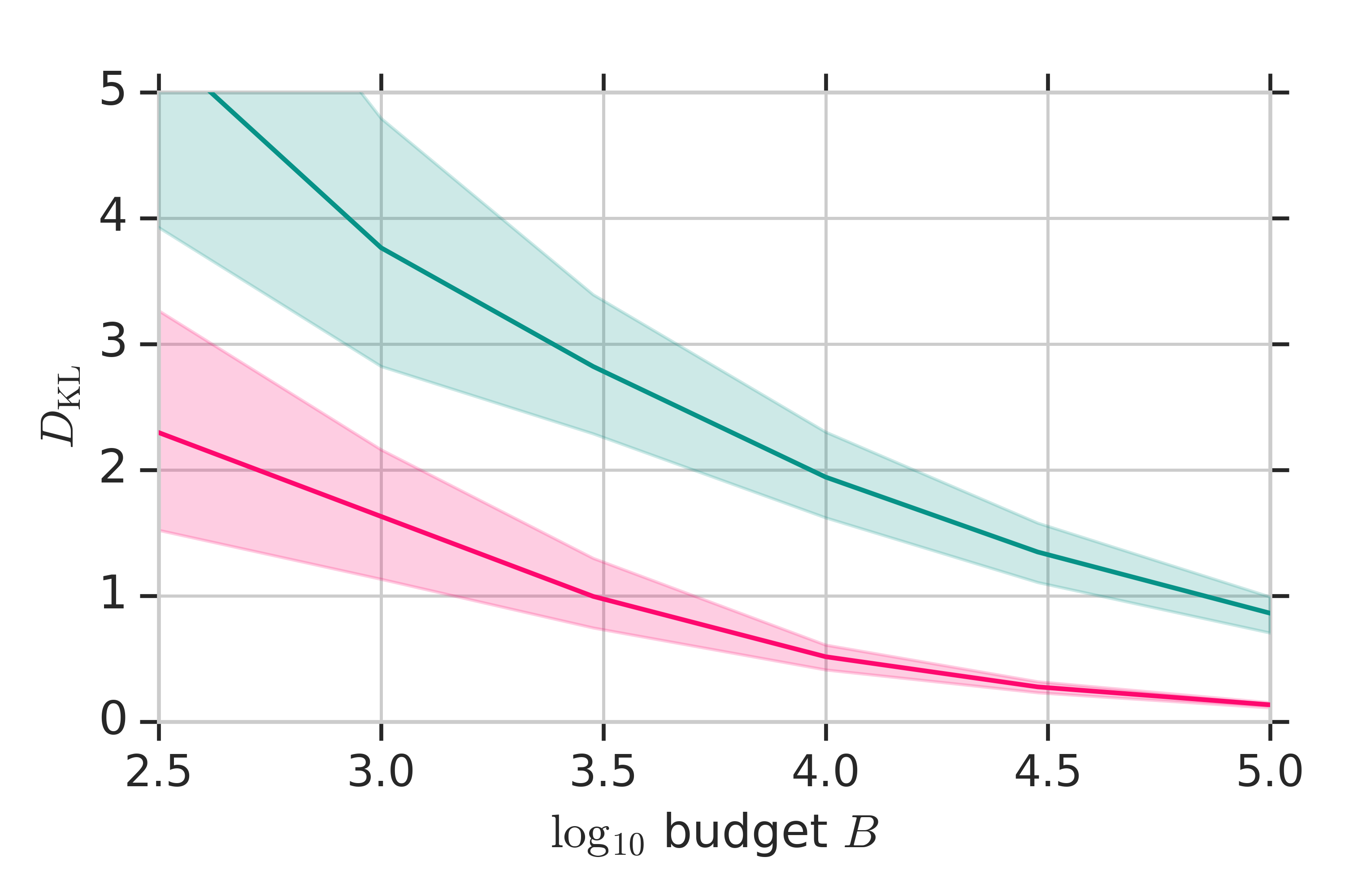
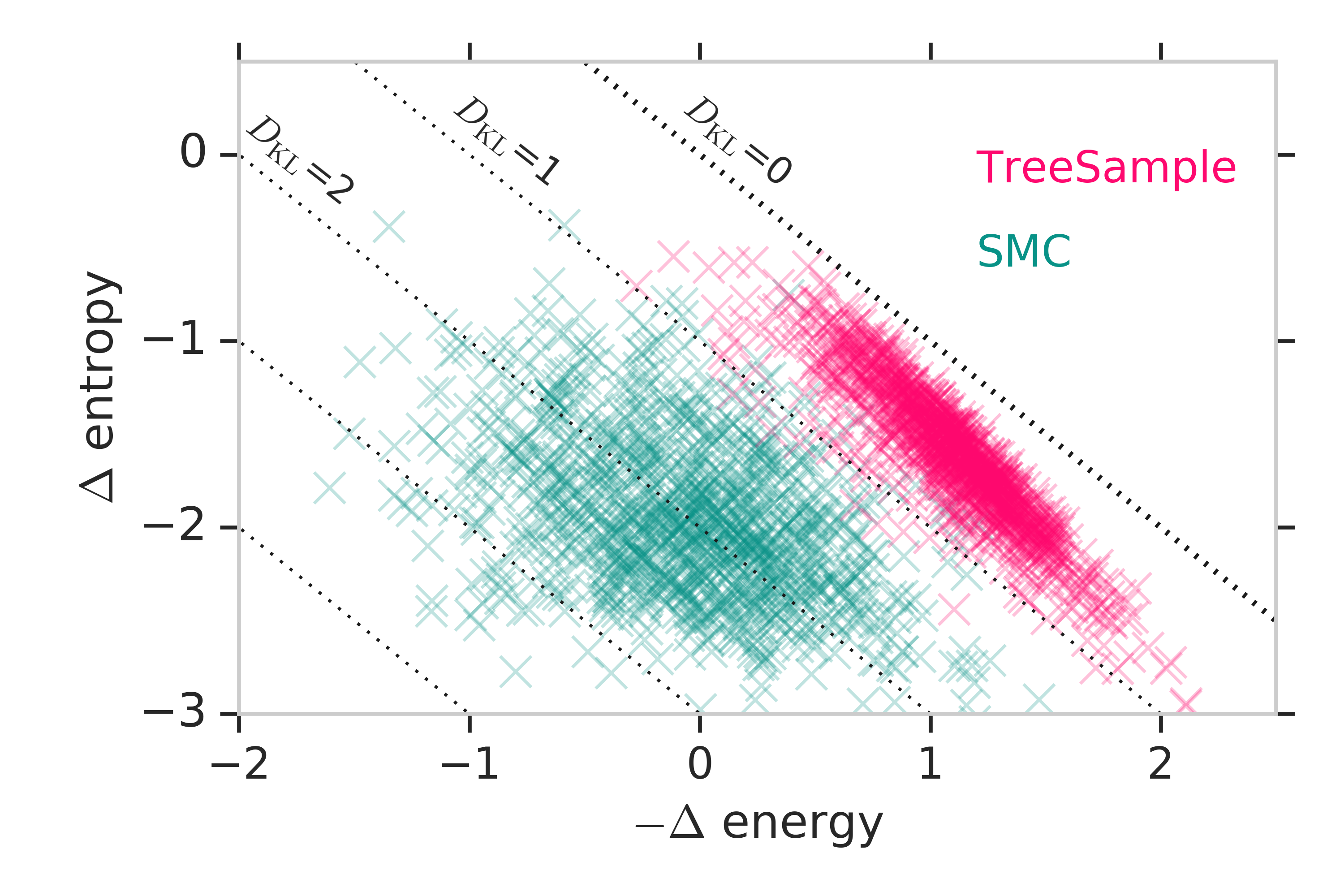
Figure 1: Comparison of TreeSample to SMC on inference in 1000 randomly generated Markov chains. Left: Approximation error $D_{\mathrm{KL}}[P_{X}\|P^{\ast}_{X}]$ as a function of the budget $B$ in log-scale, showing that SCM needs more than 30 times the budget of TreeSample to generate comparable approximations. Right: Energy and entropy contributions to the $D_{\mathrm{KL}}[P_{X}\|P^{\ast}_{X}]$ for all 1000 experiments for $B=10^{4}$, showing that TreeSample finds approximations with both higher entropy and lower energy.

In the following, we empirically compare TreeSample to other baseline inference methods on different families of distributions. We quantify approximation error by the Kullback-Leibler divergence:

$$D_{\mathrm{KL}}[P_{X}\|P^{\ast}_{X}]= \log Z \underbrace{-\mathbb{E}_{P_{X}}\left[\sum_{m=1}^{M}\psi_{m}(X)\right]-\mathbb{H}\left[P_{X}\right]}_{:=}$$ (8)

$$= \log Z +\ \ \ \ \ \ \ \Delta D_{\mathrm{KL}}[P_{X}\|P^{\ast}_{X}],$$

where we refer to the second term in eqn. 8 as negative expected energy, and the last term is the entropy of the approximation. We can get unbiased estimates of these using samples from $P_{X}$. For intractable target distributions, we compare different inference methods using $\Delta D_{\mathrm{KL}}:=D_{\mathrm{KL}}-\log Z$, which is tractable to approximate and preserves ranking of different approximation methods.

As baselines we consider the following: Sequential Importance Sampling (SIS), Sequential Monte Carlo (SMC) and for a subset of the environments also Gibbs sampling (GIBBS) and sampling with loopy belief propagation (BP); details are given in the appendix. We use the baseline methods in the following way: We generate a set of particles $\{x^{i}\}_{i\leq I}$ of size $I$ such that we exhaust the budget $B$, and then return the (potentially weighted) sum of atoms $\sum_{i\leq I}p^{i}\delta(x,x^{i})$ as the approximation density; here $\delta$ is the Kronecker delta, and $p^{i}$ are either set to $1/I$ for GIBBS, BP and to the self-normalized importance weights for SIS and SMC. Hyperparameters for all methods where tuned individually for different families of distributions on an initial set of experiments and then kept constant across all reported experiments. For further details, see the appendix. For SIS and SMC, the proposal distribution plays a comparable role to the state-action prior in TreeSample. Therefore, for all experiments we used the same parametric family for $Q^{\phi}$ for TreeSample, SIS and SMC.

For the sake of simplicity, in the experiments we measured and constrained the inference budget $B$ in terms of reward evaluations, i.e. each pointwise evaluate of a $R_{n}$ incurs a cost of one, instead of factor evaluations.

4.1 TreeSample  without Parametric Value Function

We first investigated inference without learned parametric $Q^{\phi}$. Instead, we used the simple heuristic of setting $\forall a\forall n\ Q^{\phi}_{n}(a|x_{<n}):=(N-n)\log K$, which corresponds to the state-action values when all factors $\psi_{m}\equiv 0$ vanish everywhere.

4.1.1 Chain Distributions

We initially tested the algorithms on inference in chain-structured factor graphs (CHAINS). These allow for exact inference in linear time, and therefore we can get unbiased estimates of the true Kullback-Leibler divergences. We report results averaged over $10^{3}$ different chains of length $N=10$ with randomly generated unary and binary potential functions; for details, see appendix. The number of states per variable was set to $K=5$, yielding $K^{N}\approx 10^{7}$ states in total. The results, shown in fig. 1 as a function of the inference budget $B$, show that TreeSample outperforms the SMC baseline (see also tab. 1). In particular, TreeSample generates approximations of similar quality compared to SMC with a roughly 30 times smaller budget. We further investigated the energy and entropy contributions to $D_{\mathrm{KL}}$ separately. We define $\Delta$energy$=\mathbb{E}_{P^{\ast}_{X}}[\sum\psi]-\mathbb{E}_{P_{X}}[\sum\psi]$ (lower is better), and $\Delta$entropy$=\mathbb{H}[P_{X}]-\mathbb{H}[P^{\ast}_{X}]$ (higher is better). Fig. 1 shows that TreeSample finds approximations that have lower energy as well as higher entropy compared to SMC.

$D_{\mathrm{KL}}$ or $\Delta D_{\mathrm{KL}}$	CHAIN	PERMUTED CHAIN	FACTOR GRAPHS 1	FACTOR GRAPHS 2
SIS	11.61 $\pm$ 1.74	9.23 $\pm$ 0.34	-21.97 $\pm$ 2.47	-31.70 $\pm$ 2.32
SMC	1.94 $\pm$ 0.48	7.08 $\pm$ 0.36	-24.09 $\pm$ 2.85	-35.90 $\pm$ 2.47
GIBBS	–	–	-18.67 $\pm$ 1.80	-25.12 $\pm$ 1.48
BP	exact	exact	-21.50 $\pm$ 0.18	-31.48 $\pm$ 0.48
TreeSample	0.53 $\pm$ 0.17	3.41 $\pm$ 0.41	-28.89 $\pm$ 1.94	-38.70 $\pm$ 2.29

Table 1: Approximation error (lower is better) for different inference methods on four distribution classes. Results are averages and standard deviations over 1000 randomly generated distributions for each class. Budget was set to $B=10^{4}$.

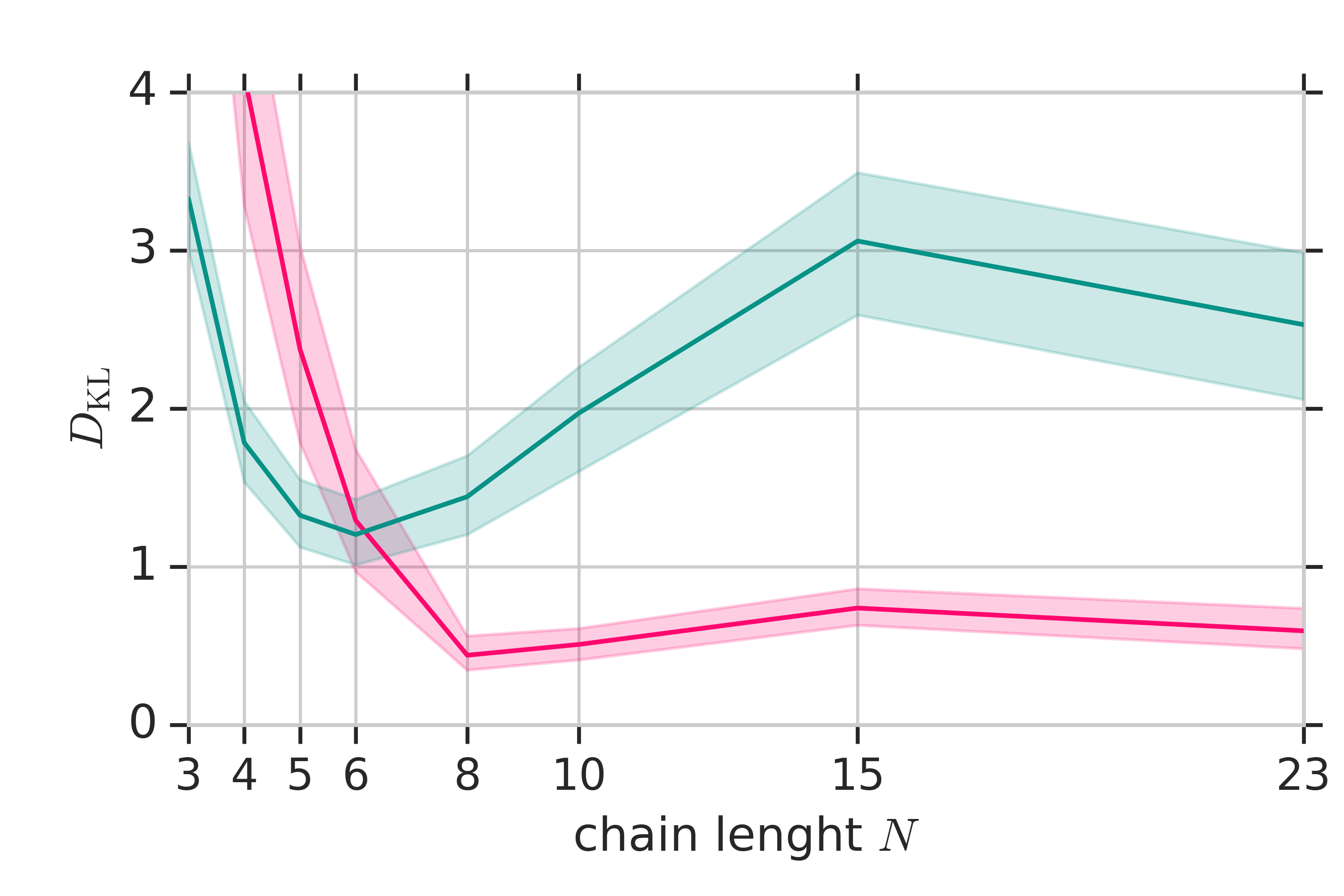
Figure 3: Approximation error for inference in chain graphs as a function of varying chain length $N$; the number $K$ of states per variable was abjusted such that the total domain size $N\log K$ stayed roughly constant. TreeSample (red) performed worse than SMC (turquoise) for short and wide chains, but performs better everywhere else.

A known limitation of tree search methods is that they tend to under-perform for shallow (here small $N$) decision-making problems with large action spaces (here large $K$). We performed experiments on chain distributions with varying $K$ and $N$ while keeping the state-space size approximately constant, i.e. $N\log K\approx\mbox{const}$. We confirmed that for very shallow, bushy problems with $\log K\gg N$, SMC outperforms TreeSample, whereas TreeSample dominates SMC in all other problem configurations, see fig. 3 in the appendix.

Next, we considered chain-structured distributions where the indices of the variables $X_{n}$ do not correspond to the ordering in the chain; we call these PermutedChains. These are in general more difficult to solve as they exhibit "delayed" rewards, i.e. binary chain potentials $\psi_{m}(X_{\sigma(n)},X_{\sigma(n+1)})$ depend on non-consecutive variables. This can create "dead-end" like situations, that SMC, not having the ability to backtrack, can get easily stuck in. Indeed, we find that SCM performs only somewhat better on this class of distributions than SIS, whereas TreeSample achieves better results by a wide margin. Results on both families of distributions are shown in tab. 1.

4.1.2 Factor Graphs

We also tested the inference algorithms on two classes of non-chain factor graphs, denoted as FactorGraphs1 and FactorGraphs2. Distributions in FactorGraphs1 are over $N=10$ variables with $K=5$ states each. Factors were randomly generated with maximum degree $d$ of 4 and their $d^{K}$ values where iid drawn from $\mathcal{N}(0,1)$. Distributions in FactorGraphs2 are over $N=20$ binary variables, i.e. $K=2$. These distributions are generated by two types of of factors: NOT (degree 2) and MAJORITY (max degree 4), both taking values in $\{0,1\}$.

Results are shown in tab. 1. For both families of distributions, TreeSample outperforms all considered baselines by a wide margin. We found that GIBBS generally failed to find configurations with high energy due to slow mixing. BP-based sampling was observed to generate samples with high energy but small entropy, yielding results comparable to SIS.

4.2 TreeSample with Parametric Value Functions

value func.	$\varnothing$	MLP	GNN
single graph	N/A	Yes	Yes	No	No	No	No
$N_{\mathrm{train}}$	N/A	20	20	20	12	16	24
$Q^{\phi}$ trained by SMC: $\Delta D_{\mathrm{KL}}^{\phi}$	–	+1.63	-0.19	-0.97	-1.00	-1.17	-0.64
	–	[-1.60,+2.87]	[-2.68,+1.49]	[-2.41,+0.40]	[-1.52, -0.58]	[-1.42,-0.46]	[-0.84,-0.32]
$Q^{\phi}$ + SMC: $\Delta D_{\mathrm{KL}}$	+2.72	+2.93	+1.64	+2.56	+2.00	+1.64	+2.10
	[1.02, 4.54]	[-1.54,+4.32]	[-1.61,+3.46]	[+0.58,+4.42]	[+1.72, +2.19]	[+1.38,+2.05]	[+1.50,+2.68]
$Q^{\phi}$ trained by TreeSample: $\Delta D_{\mathrm{KL}}^{\phi}$	–	-3.61	-3.86	-2.05	-2.12	-2.52	-1.83
	–	[-5.73,-0.60]	[-6.03, -0.85]	[-3.58, -0.55]	[-2.23,-1.99]	[-2.63,-2.40]	[-2.13,-1.76]
$Q^{\phi}$ + TreeSample: $\Delta D_{\mathrm{KL}}$	0.00	-3.63	-3.87	-2.23	-2.22	-2.64	-2.35
	[-1.47, 1.68]	[-5.72,-0.64]	[-6.05, -0.88]	[-3.75, -0.73]	[-2.30,-2.05]	[-2.79,-2.55]	[-2.46,-2.10]

Table 2: Approximation error for inference in factor graphs with TreeSample and SMC, for different types of value functions and training regimes. Results are relative to TreeSample w/o value function, lower is better. See main text for details.

Next, we investigated the performance of TreeSample, as well as SMC, with additional parametric state-action value functions $Q^{\phi}$ (used as proposal for SMC). We focused on inference problems from FactorGraphs2. We implemented the inference algorithm as a distributed architecture consisting of a worker and a learner process, both running simultaneously. The worker requests an inference problem instance, and performs inference either with TreeSample or SMC with a small budget of $B=2500$ using the current parametric $Q^{\phi}$. After building the approximation $P_{X}$, 128 independent samples $x^{i}\sim P_{X}$ are drawn from it and the inferred $Q$-values $Q_{n}(\cdot|x^{i}_{\leq n})$ for $i=1,\ldots,128$ and $n=1,\ldots,N$ are written into a replay buffer as training data; following this, the inference episode is terminated, the tree is flushed and a new episode starts. The learner process samples training data from the replay for updating the parametric $Q^{\phi}$ with an SGD step on a minibatch of size 128; then the updated model parameters $\phi$ are sent to the worker. We tracked the error of the inference performed on the worker using the unnormalized $\Delta D_{\mathrm{KL}}$ as a function of the number of completed inference episodes. We expect $\Delta D_{\mathrm{KL}}$ to decrease, as $Q^{\phi}$ adapts to the inference problem, and therefore becomes better at guiding the search. Separately, we also track the inference performance of only using the value function $Q^{\phi}$ without additional search around it, denoted as $\Delta D_{\mathrm{KL}}^{\phi}$. This is a purely parametric approximation to the inference problem, trained by samples from TreeSample and SMC respectively. We observed that $\Delta D_{\mathrm{KL}}$ as well as $\Delta D_{\mathrm{KL}}^{\phi}$ stabilized after roughly 1500 inference episodes for all experiments. Results were then averaged over episodes 2000-4000 and are shown in tab. 2. To facilitate comparison, all results in tab. 2 are reported relative to $\Delta D_{\mathrm{KL}}$ for TreeSample without value functions. In general, experimental results with learned value functions exhibited higher degrees of variability with some outliers. Results in tab. 2 therefore report median results over 20 runs as well as 25% and 75% percentiles.

We first performed a simple set of "sanity-check" experiments on TreeSample with parametric value functions in a non-transfer setting, where the worker repeatedly solves the same inference problem arising from a single factor graph. As value function, we used a simple MLP with 4-layers and 256 hidden units each. As shown in the second column of tab. 2, approximation error $\Delta D_{\mathrm{KL}}$ decreases significantly compared to plain TreeSample without value functions. This corroborates that the value function can indeed cache part of the previous search trees and facilitate inference if training and testing factor graphs coincide. Furthermore, we observed that once $Q^{\phi}$ is fully trained, the inference error $\Delta D_{\mathrm{KL}}^{\phi}$ obtaind using only $Q^{\phi}$ is only marginally worse than $\Delta D_{\mathrm{KL}}$ using $Q^{\phi}$ plus TreeSample-search on top of it; see row four and five in tab. 2 respectively. This indicates that the value function was powerful enough in this experiment to almost cache the entire search computation of TreeSample.

Next, we investigated graph neural networks (GNNs) [29] as value functions $Q^{\phi}$. This function class can make explicit use of the structure of the factor graph instances. Details about the architecture can be found in [29] and the appendix, but are briefly described in the following. GNNs consist of two types of networks, node blocks and edge blocks (we did not use global networks), that are connected according to the factor graph at hand, and executed multiple times mimicking a message-passing like procedure. We used three node block networks, one for each type of graph node, i.e. variable node (corresponding to a variable $X_{n}$), NOT-factors and MAJORITY-factors. We used four edge block networks, namely one for each combination of {incoming,outgoing}$\times${NOT, MAJORITY}. Empirically, we found that GNNs slightly outperform MLPs in the non-transfer setting, see third column of tab. 2.

The real advantage of GNNs comes into play in a transfer setting, when the worker performs inference in a new factor graph for each episode. We keep the number of variables fixed ($N_{\mathrm{train}}=N_{\mathrm{test}}=20$) but vary the number and configuration of factors across problems. GNNs successfully generalize across graphs, see fourth column of tab. 2. This is due to their ability to make use of the graph topology of a new factor graph instance, by connecting its constituent node and edge networks accordingly. Furthermore, the node and edge networks evidently learned generic message passing computations for variable nodes as well as NOT/MAJORITY factor nodes. The results show that a suitable $Q^{\phi}$ generalizes knowledge across inference problems, leading to less approximation error on new distributions. Furthermore, we investigated a transfer setting where the worker solves inference problems on factor graphs of sizes $N_{\mathrm{train}}=12,16$ or 24, but performance is tested on graphs of size $N_{\mathrm{test}}=20$; see columns five to seven in tab. 2. Strikingly, we find that the value functions generalize as well across problems of different sizes as they generalize across problems of the same size. This demonstrates that prior knowledge can successfully guide the search and greatly facilitate inference.

Finally, we investigated the performance of SMC with trained value functions $Q^{\phi}$; see rows one and two in tab. 2. Overall, we found that performance was worse compared to TreeSample: Value functions $Q^{\phi}$ trained by SMC were found to give worse results $\Delta D_{\mathrm{KL}}^{\phi}$ compared to those trained by TreeSample, and overall inference error was worse compared to TreeSample. Interestingly, we found that once $Q^{\phi}$ is fully trained, performing additional SMC on top of it made results worse. Although initially counter-intuitive, these results are sensible in our problem setup. The entropy of SMC approximations $\approx\log I$ is essentially given by the number of particles $I$ that SMC produces; this number is limited by the budget $B$ that can be used to compute importance weights. Once a parametric $Q^{\phi}$ is trained, it does not need to make any further calls to the $\psi_{m}$ factors, and can therefore exhibit much higher entropy, therefore making $\Delta D_{\mathrm{KL}}^{\phi}$ smaller than $\Delta D_{\mathrm{KL}}$.

5 Related Work

TreeSample is based on the connection between probabilistic inference and maximum-entropy decision-making problems established by previous work. This connection has mostly been used to solve RL problems with inference methods e.g. [20, 32, 33, 21]. Closely related to our approach, this relationship has also been used in the reverse direction, i.e. to solve inference problems using tools from RL [34, 22, 23, 24, 25], however without utilizing tree search and emphasizing the importance of exploration for inference. The latter has been recognized in [19], and applied to hierarchical partitioning for inference in continuous spaces, see also [35]. In contrast to this, we focus on discrete domains with sequential decision-making utilizing MCTS and value functions. Soft-Bellman backups, as used here (also referred to as soft Q-learning) and their connection to entropy-regularized RL have been explored in e.g. [36, 37].

For approximating general probabilistic inference problems, the class of Markov Chain Monte Carlo (MCMC) methods has proven very successful in practice. There, a transition operator is defined such that the target distribution is stationary under this operator. Concretely, MCMCs methods operate on a fully specified, approximate sample which is then perturbed iteratively. Transition operators are usually designed specifically for families of distributions in order to leverage problem structure for achieving fast mixing. However, mixing times are difficult to analyze theoretically and hard to monitor in practice [38]. TreeSample circumvents the mixing problem by generating a new sample "from scratch" when returning to the root node and then iteratively stepping through the dimensions of the random vector. Furthermore, TreeSample can make use of powerful neural networks for approximating conditionals of the target, thus caching computations for related inference problems. Although, adaptive MCMC methods exist, they usually only consider small sets of adaptive parameters [18]. Recently, MCMC methods have been extended to transition operators generated by neural networks, which are trained either by adversarial training, meta learning or mixing time criteria [39, 40, 41, 42]. However, these were formulated for continuous domains and rely on differentiability and thus do not carry over straight-forward to discrete domains.

Our proposed algorithm is closely related to Sequential Monte Carlo (SMC) methods [13], another class of broadly applicable inference algorithms. Often, these methods are applied to generate approximate samples by sequentially sampling the dimensions of a random vector, e.g. in particle filtering for temporal inference problems [43]. Usually, these methods do not allow for backtracking, i.e. re-visiting previously discarded partial configurations, although few variants with some back-tracking heuristics do exist [44, 45]. This is contrast to the TreeSample algorithm, which decides at every iteration where to expand the current tree based on a full tree-traversal from the root and therefore allows for backtracking an arbitrary number of steps. Furthermore, we propose to train value functions which approximately marginalize over the "future" (i.e. variables following the one in question in the ordering), thus taking into account relevant downstream effects. [46, 47] introduce adaptive NN proposals, i.e. value functions in our formulation, but these are trained to match the "filtering" distribution, thus they do not marginalize over the future. In the decision-making formulation, this corresponds to learning proposals based on immediate rewards instead of total returns. However, recent work in continuous domains has begun to address this [48, 49, 50, 51], however, they do not make use of guided systematic search.

Recently, distilling inference computations into parametric functions as been extended to discrete distributions based on the framework of variational inference. [34, 52] highlight connections to the REINFORCE gradient estimator [53] and propose various value function-like control variates for reducing its variance. Multiple studies propose to utilize continuous relaxation of discrete variables to make use of so-called reparametrization gradients for learning inference computations, e.g. [54].

In addition to the approximate inference methods discussed above, there are numerous algorithms for exact inference in discrete models. One class of methods called Weighted Model Counting (WMC) algorithms, is based on representing the target probability distribution as Boolean formulas with associated weights, and convert inference into the problem of summing weights over satisfying assignments of the associated SAT problem [55]. In particular, it has been shown that DPLL-style SAT solvers [56] can be extended to exactly solve general discrete inference problems [57, 58], often outperforming other standard methods such as the junction tree algorithm [59]. Similar to TreeSample, this DPLL-based approach performs inference by search, i.e. it recursively instantiates variables of the SAT problem. Efficiency is gained by chaching solved sub-problems [60] and heuristics for adaptively choosing the search order of variables [57]. We expect that similar techniques could be integrated into the TreeSample algorithm, potentially greatly improving its efficiency. In contrast to WMC methods, TreeSample dynamically chooses the most promising sub-problems to spend compute on via the UCT-like selection rule which is informed by all previous search tree expansions.

6 Discussion

Structured distributions $P^{\ast}_{X}$, such as factor graphs, Bayesian networks etc, allow for a very compact representation of an infinitely large set of beliefs, e.g. $P^{\ast}_{X}$ implies beliefs over $f(X)$ for every test function $f$, including marginals, moments etc. This immediately raises the question: "What does it mean to ’know’" a distribution? (paraphrased from [61]). Obviously, we need to perform probabilistic inference to "convert the implicit knowledge" of $P^{\ast}_{X}$ (given by e.g. factors) into "explicit knowledge" in terms of the beliefs of interest (quoted from [62]). If the dimension of $X$ is anything but very small, this inference process cannot be assumed to be "automatic", but ranks among the most complex computational problems known, and large amounts of computational resources have to be used to just approximate the solution. In other challenging computational problems such as optimization, integration or solving ordinary differential equations, it has been argued that the results of computations that have not yet been executed are to be treated as unobserved variables, and knowledge about them to be expressed as beliefs [63, 61]. This would imply for the inference setting considered in this paper, that we should introduce second-order, or meta-beliefs over yet-to-be-computed first-order beliefs implied by $P^{\ast}_{X}$. Approximate inference could then proceed analogously to Bayesian optimization: Evaluate the factors of $P^{\ast}_{X}$ at points that result in the largest reduction of second-order uncertainty over the beliefs of interest. However, it is unclear how such meta-beliefs can be treated in a tractable way. Instead of such a full Bayesian numerical treatment involving second-order beliefs, we adopted cheaper Upper Confidence Bound heuristics for quantifying uncertainty.

For sake of simplicity, we assumed in this paper that the computational cost of inference is dominated by evaluations of the factor oracles. This assumption is well justified e.g. in applications, where some factors represent large scale scientific simulators [6], or in modern deep latent variable models, where a subset of factors is given by deep neural networks that take potentially high-dimensional observations as inputs. If this assumption is violated, i.e. all factors can be evaluated cheaply, the comparison of TreeSample to SMC and other inference methods will become less favourable for the former. TreeSample incurs an overhead for traversing a search tree before expanding it, attempting to use the information of all previous oracle evaluations. If these are cheap, a less sequential and more parallel approach, such as SMC, might become more competitive.

We expect that TreeSample can be improved and extended in many ways. Currently, the topology of the factor graph is only partially used for the reward definition and potentially for graph net value functions. One obvious way to better leverage it would be to check if after conditioning on a prefix $x_{<n}$, corresponding to a search depth $n$, the factor graph decomposes into independent components that can be solved independently. Furthermore, TreeSample uses a fixed ordering of the variables. However, a good variable ordering can potentially make the inference problem much easier. Leveraging existing or developing new heuristics for a problem-dependent and dynamic variable ordering could potentially increase the inference efficiency of TreeSample.

Appendix A Details for TreeSample  algorithm

We define a search tree $\mathcal{T}$ in the following way. Nodes in $\mathcal{T}$ at depth $n\in\{0,1,\ldots,N\}$ are indexed by the (partial) state $x\in\{1,\ldots,K\}^{n}$, and the root is denoted by $\varnothing$. Each node $x$ at depth $n=len(x)$ keeps track of the corresponding reward evaluation $R_{n}(x)$ and the following quantities for all its children:

1. visit counts $\eta_{n+1}(\cdot|x)=(\eta_{n+1}(1|x),\ldots,\eta_{n+1}(K|x))\in\mathbb{N}^{K}$ over the children,

2. state-action values $Q_{n+1}(\cdot|x)\in\mathbb{R}^{K}$,

3. prior state-action values $Q^{\phi}_{n+1}(\cdot|x)\in\mathbb{R}^{K}$, and

4. a boolean vector $C_{n+1}(\cdot|x)\in\{0,1\}^{K}$ if its children are complete (i.e. fully expanded, see below).

Standard MCTS with (P)UCT-style tree traversals applied to the inference problem can in general visit any state-action pair multiple times; this is desirable behavior in general MDPs with stochastic rewards, where reliable reward estimates require multiple samples. However, the reward $R$ in our MDP is deterministic as defined in eqn. 2, and therefore there is no benefit in re-visiting fully-expanded sub-trees. To prevent the TreeSample algorithm from doing so, we explicitly keep track at each node if the sub-tree rooted in it is fully-expanded; such a node is called complete. Initially no internal node is complete, only leaf nodes at depth $N$ are tagged as complete. In the backup stage of the tree-traversal, we tag a visited node as complete if it is a node of depth $N$ (corresponding to a completed sample) or if all its children are complete. We modify the action selection eqn. 7 such that the $\operatorname*{arg\,max}$ is only taken over actions not leading to complete sub-trees. The TreeSample algorithm is given in full in algorithm 2.

Algorithm 2 TreeSample  procedures

1:globals reward function $R$, prior state-action value function $Q^{\phi}$

2:procedure TreeSample(budget B)

3:    initialize empty tree $\mathcal{T}\leftarrow\varnothing$

4:    available budget $b\leftarrow B$

5:    while $b>M$ do

6:         $\mathcal{T},\Delta b$  $\leftarrow$ TreeTravsersal ($\mathcal{T}$)

7:         $b\leftarrow b-\Delta b$

8:    end while

9:    return tree $\mathcal{T}$

10:end procedure

11:procedure TreeTraversal(tree $\mathcal{T}$)

12:      // traversal

13:    $x\leftarrow\varnothing$

14:    while $x\in\mathcal{T}$ do

15:         $n\leftarrow len(x)$

16:         $a\leftarrow$ Q-UCT$(\eta_{n+1}(\cdot|x),Q_{n+1}(\cdot|x),Q_{n+1}^{\phi}(\cdot|x),C_{n+1}(\cdot|x))$

17:         $x\leftarrow x\circ a$

18:    end while

19:      // expansion

20:    if $x\not\in\mathcal{T}$ then

21:         $\mathcal{T}\ \leftarrow\ \mathcal{T}\ \cup$  Expand$(x)$

22:         used budget $\Delta b\leftarrow|M_{n}|$      // see def. 1

23:    end if

24:      // backup

25:    for $n=len(x),\ldots,1,0$ do

26:         $V_{n+1}(x_{\leq n})=\log\sum_{a^{\prime}=1}^{K}\exp Q_{n+1}(a^{\prime}|x_{\leq n})$

27:         $Q_{n}(x_{n}|x_{<n})\leftarrow R_{n}(x_{n}|x_{<n})+V_{n+1}(x_{\leq n})$

28:         $C_{n}(x_{n}|x_{<n})\leftarrow\min_{a^{\prime}}C_{n+1}(a^{\prime}|x_{\leq n})$

29:         $\eta_{n}(x_{n}|x_{<n})\leftarrow\eta_{n}(x_{n}|x_{<n})+1$

30:    end for

31:    return $\mathcal{T}$, $\Delta b$

32:end procedure

33:procedure Q-UCT($\eta_{n+1}(\cdot|x)$, $Q_{n+1}(\cdot|x)$, $Q_{n+1}^{\phi}(\cdot|x)$, $C_{n+1}(\cdot|x)$)

34:    return $\operatorname*{arg\,max}$ of eqn. 7 over in-complete children $\{a|C_{n+1}(a|x)=0\}$

35:end procedure

36:procedure Expand(state $x$)

37:    $n\leftarrow len(x)$

38:    evaluate reward function $R_{n}(x_{n}|x_{<n})$

39:    initialize $\eta_{n+1}(\cdot|x)\leftarrow(0,\ldots,0)$

40:    if $n=N$ then    // $x$ is leaf

41:         initialize $Q_{n+1}(a\cdot|x)\leftarrow-\log K$ for all $a\in\{1,\ldots,K\}$

42:         initialize $C_{n+1}(\cdot|x)\leftarrow(1,\ldots,1)$

43:    else

44:         evaluate prior $Q_{n+1}^{\phi}(\cdot|x)$

45:         initialize $Q_{n+1}(\cdot|x)\leftarrow Q_{n+1}^{\phi}(\cdot|x)$

46:         initialize $C_{n+1}(\cdot|x)\leftarrow(0,\ldots,0)$

47:    end if

48:    return node $x$ with $\eta_{n+1}(\cdot|x)$, $Q_{n+1}(\cdot|x)$, $Q_{n+1}^{\phi}(\cdot|x)$, $C_{n+1}(\cdot|x)$, $R_{n}(x_{n}|x_{<n})$

49:end procedure

Appendix B Proofs

B.1 Observation 2

Proof.

This observation has been proven previously in the literature, but we will give a short proof here for completeness. We show the statement by determining the optimal policy and value function by backwards dynamic programming (DP). We anchor the DP induction by defining the optimal value function at step $N+1$ as zero, i.e. $V^{\ast}_{N+1}(x_{\leq N})=0$. Using the law of iterated expectations, we can decompose the optimal value function in the following way for any $n=N,\ldots,1$:

$$V^{\ast}_{n}(x_{<n}) = \max_{\pi_{n},\ldots,\pi_{N}}\ \mathbb{E}_{P^{\pi}_{X_{\geq n}|x_{<n}}}\left[\sum_{n^{\prime}=n}^{N}R_{n^{\prime}}-\log\pi_{n^{\prime}}\right]$$

$$= \max_{\pi_{n}}\ \mathbb{E}_{P^{\pi}_{X_{n}|x_{<n}}}\ \max_{\pi_{n+1},\ldots,\pi_{N}}\ \mathbb{E}_{P^{\pi}_{X_{>n}|x_{<n}\circ X_{n}}}\left[\sum_{n^{\prime}=n}^{N}R_{n^{\prime}}-\log\pi_{n^{\prime}}\right]$$

$$= \max_{\pi_{n}}\ \mathbb{E}_{P^{\pi}_{X_{n}|x_{<n}}}\left[R_{n}-\log\pi_{n}+\max_{\pi_{n+1},\ldots,\pi_{N}}\mathbb{E}_{P^{\pi}_{X_{>n}|x_{<n}\circ X_{n}}}\left[\sum_{n^{\prime}=n+1}^{N}R_{n^{\prime}}-\log\pi_{n^{\prime}}\right]\right]$$

$$= \max_{\pi_{n}}\ \mathbb{E}_{P^{\pi}_{X_{n}|x_{<n}}}\ \left[R_{n}-\log\pi_{n}+V^{\ast}_{n+1}\right].$$

Therefore, assuming by induction that $V^{\ast}_{n+1}$ has been computed, we can find the optimal policy $\pi^{\ast}_{n}$ and value $V^{\ast}_{n}$ at step $n$ by solving:

$$\operatorname*{arg\,max}_{f:\{1,\ldots,K\}\rightarrow[0,1]} \sum_{a=1}^{K}f(a)\cdot\left(R_{n}(x_{<n}\circ a)-\log f(a)+V^{\ast}_{n+1}(x_{<n}\circ a)\right)$$ (9a)

subject to $$\sum_{a=1}^{K}f(a)=1.$$ (9b)

The solution to this optimization problem can be found by the calculus of variations (omitted here) and is given by:

$$\log\pi^{\ast}(x_{n}|x_{<n}) \propto R_{n}(x_{\leq n})+V_{n+1}^{\ast}(x_{\leq n})=Q^{\ast}_{n}(x_{n}|x_{<n}),$$

where we used the definition of the optimal state-action value function. Furthermore, at the optimum, the objective eqn. 9a assumes the value:

$$V^{\ast}_{n}(x_{<n}) = \log\sum_{x_{n}=1}^{K}\exp Q_{n}^{\ast}(x_{n}|x_{<n}).$$

This expression, together with the definition of $Q^{\ast}$ establishes the soft-Bellman equation. The optimal value $V^{\ast}_{n+1}$ is also exactly the log-normalizer for $\pi^{\ast}_{n}$. Therefore, we can write:

$$\log\pi^{\ast}_{n}(x_{n}|x_{<n})=Q^{\ast}_{n}(x_{n}|x_{<n})-V^{\ast}_{n+1}(x_{\leq n}).$$

∎

B.2 Proof of Lemma 1

Proof.

We will show this statement by induction on the depth $d:=N-n$ of the sub-tree $\mathcal{T}_{x_{\leq n}}$ with root $x_{\leq n}$. For $d=0$, i.e. $n=N$, the state-action values $Q_{N+1}(\cdot|x_{\leq N}):=-\log K$ are defined such that $V_{N+1}(x_{\leq N})=0$, which is the correct value. Consider now the general case $1\leq d\leq N$. Let $\mathcal{T}^{\prime}_{x_{\leq n}}$ be the sub-tree before the last tree traversal that expanded the last missing node $x_{\leq N}$, ie $\mathcal{T}_{x_{\leq n}}=\mathcal{T}^{\prime}_{x_{\leq n}}\cup x_{\leq N}$; for an illustration see fig. 2. The soft-Bellman backups of the last completing tree-traversal on the path leading to $x_{\leq N}$ are by construction all of the following form: For any node $x_{\leq m}$ on the path, all children except for one correspond to already completed sub-trees (before the last traversal). The sub-tree of the one remaining child is completed by the last traversal. All complete sub-trees on the backup path are of depth smaller than $d$ and therefore by induction their roots have the correct values $V_{m+1}^{\ast}(x_{\leq m})$. Hence evaluating the soft-Bellman backup eqn. 6 (with the true noiseless reward $R$) yields the correct value for $x_{\leq n}$. ∎

Appendix C Details for Experiments

C.1 Baseline Inference Methods

C.1.1 SIS and SMC

For each experiment we determined the number of SIS and SMC particles $I$ such that the entire budget $B$ was used. We implemented SMC with an resampling threshold $t\in[0,1]$, i.e. a resampling step was executed when the effective sample size (ESS) was smaller than $tI$. The threshold $t$ was treated as a hyperparameter; SMC with $t=0$ was used as SIS results.

C.1.2 BP

We used the algorithm outline on p. 301 from [64]. For generating a single approximate sample from the target, the following procedure was executed. Messages from variable to factor nodes were initialized as uniform; then $N_{message}$ message-passing steps, each consisting of updating factor-variable and variable-factor messages were performed. $X_{1}$ was then sampled form the resulting approximate marginal, and the messages from $X_{1}$ to its neighboring factors were set to the corresponding atom. This was repeated until all variables $X_{n}$ were sampled, generating one approximate sample from the joint $P^{\ast}_{X}$.

In total, we generated multiple samples with the above algorithm such that the budget $B$ was exhausted. The number $N_{message}$ of message-passing steps before sampling each variable $X_{n}|X_{<n}$ was treated as a hyperparameter.

C.1.3 GIBBS

We implemented standard Gibbs sampling. All variables were initially drawn uniformly from $\{1,\ldots,K\}$ , and $N_{Gibbs}$ iterations, each consisting of updating all variables in the fixed order $X_{1}$ to $X_{N}$, were executed. This generated a single approximate sample. We repeated this procedure to generate multiple samples such that the budget $B$ was exhausted. We treated $N_{Gibbs}$ as a hyperparameter.

C.2 Hyperparameter optimization

For each inference method (except for SIS) we optimized one hyperparameter on a initial set of experiments. For TreeSample, we fixed $\epsilon=0.1$ and optimized $c$ from eqn. 7. Different hyperparameter values were used for different families of distributions. Hyperparameters were chosen such as to yield lowest $\Delta D_{\mathrm{KL}}$.

C.3 Details for Synthetic Distributions

C.3.1 Chains

The unary potentials $\psi_{n}(x_{n})$ for $n=1,\ldots,N$ for the chain factor graphs where randomly generated in the following way. The values of $\psi_{n}(x_{n}=k)$ for $n=1,\ldots,N$ and $k=1,\ldots,K$ where jointly drawn from a GP over the two dimensional domain $\{1,\ldots,N\}\times\{1,\ldots,K\}$ with an RBF kernel with bandwidth 1 and scale 0.5. Binary potentials $\psi_{n,n+1}(x_{n},x_{n+1})$ were set to $2.5\cdot d(x_{n},x_{n+1})$, where $d(x_{n},x_{n+1})$ is the distance between $x_{n}$ and $x_{n+1}$ on the 1-d torus generated by constraining $1$ and $K$ to be neighbors.

C.3.2 PermutedChains

We first uniformly drew random permutations $\sigma:\{1,\ldots,N\}\rightarrow\{1,\ldots,N\}$. We then randomly generated conditional probability tables for $P^{\ast}_{X_{\sigma(n)}|x_{\sigma({n-1})}}$ by draws from a symmetric Dirichlet with concentration parameter $\alpha=1$. These were then used as binary factors.

C.3.3 FactorGraphs1

We generated factor graphs for this family in the following way. First, we constructed Erdős-Rényi random graphs with $N$ nodes with edge probability $p=2\log(N)/N$; graphs with more than one connected component were rejected. For each clique in this graph we inserted a random factor and connected it to all nodes in the clique; graphs with cliques of size $>4$ where rejected.

For applying the sequential inference algorithms TreeSample, SIS and SMC, variables in the graph were ordered by a simple heuristic. While iterating over factors in order of descending degree, all variables in the current factor were were added to the ordering until all were accounted for.

C.3.4 FactorGraphs2

We generated factor graphs for this family over binary random variables $K=2$ in the following way. Variables $X_{2n+1}$ and $X_{2(n+1)}$ for $n=0,\ldots,N/2-1$ were connected with a NOT factor, which carries out the computation $XOR(X_{2n+1},X_{2(n+1)})$. We then constructed Erdős-Rényi random graphs of size $N/2$ over all pairs of nodes $(X_{2n+1},X_{2(n+1)})$ with edge probability $p=3\log(N/2)/N$; graphs with more than one connected component were rejected. For each clique in this intermediate graph we inserted a MAJORITY factor and connected it to either to $X_{2n+1}$ or $X_{2(n+1)}$; graphs with cliques of size $>4$ where rejected. MAJORITY factors return a value of 1.0 if half or more nodes in its neighborhood are 2 and return 0 otherwise. The output values of all factors were also scaled by 2.0; otherwise the resulting distributions were found to be very close to uniform.

C.4 Details For Experiments w/ Value Functions

All neural networks were trained with the ADAM optimizer [65] with a learning rate of $3\cdot 10^{-4}$ and mini-batches of size 128. The replay buffer size was set to $10^{4}$.

The MLP value function used for the experiment consisted of 4 hidden layers with 256 units each with RELU activation functions. Increasing the number of units or layers did not improve results.

The GNN value function $Q^{\phi}(\cdot|x_{\leq n})$ was designed as follows. Each variable node in the factor graph was given a $(16+K)$-dimensional feature vector, and each edge node a $16$-dimensional feature vector. The input prefix $x_{\leq n}$ was encoded in a one-hot manner in the first $K$ components of the variable feature vectors for variables up to $n$; for variables $>n$ the first $K$ components were set to 0. All edge features were initialized to 0. All node and edge block networks where chosen to be MLPs with 3 hidden layers and 16 units each with RELU activations. Results did not improve with deeper or wider networks. The resulting GNN was iterated 4 times; interestingly more iterations actually reduced final performance somewhat. The output feature vector of the GNN at variable node $x_{n}$ was then passed to a linear layer with $K$ outputs yielding the vector $(Q^{\phi}(x_{n+1}=1|x_{\leq n}),\dots,Q^{\phi}(x_{n+1}=K|x_{\leq n}))$.

Figure 2: Completing a sub-tree yields the exact $Q$-value. Assume the tree traversal shown in blue completes the sub-tree $\mathcal{T}_{x_{\leq n}}$ rooted in $x_{\leq n}$. Then, by construction, the soft-Bellmann backups along this path, at every intermediate node $x_{\leq m}$ for $m>n$, take as input the values of all children. By construction, all but one children correspond to complete sub-trees of a smaller depth; these have the correct values by induction. The other remaining child corresponds to a sub-tree that was completed by the last traversal and therefore has also the correct value.

References

- [1] Richard T Cox. Probability, frequency and reasonable expectation. American journal of physics, 14(1):1–13, 1946.
- [2] Edwin T Jaynes. Probability theory: The logic of science. Cambridge university press, 2003.
- [3] AM Turing. The applications of probability to cryptography. Report, GCHQ, Cheltenham, UK, 1941.
- [4] Robert J McEliece, David JC MacKay, and Jung-Fu Cheng. Turbo decoding as an instance of Pearl’s “belief propagation” algorithm. IEEE Journal on selected areas in communications, 16(2):140–152, 1998.
- [5] Mark D Robinson, Davis J McCarthy, and Gordon K Smyth. edgeR: a Bioconductor package for differential expression analysis of digital gene expression data. Bioinformatics, 26(1):139–140, 2010.
- [6] Atılım Güneş Baydin, Lei Shao, Wahid Bhimji, Lukas Heinrich, Lawrence Meadows, Jialin Liu, Andreas Munk, Saeid Naderiparizi, Bradley Gram-Hansen, Gilles Louppe, et al. Etalumis: Bringing Probabilistic Programming to Scientific Simulators at Scale. arXiv preprint arXiv:1907.03382, 2019.
- [7] Diederik P Kingma and Max Welling. Auto-encoding variational Bayes. arXiv preprint arXiv:1312.6114, 2013.
- [8] Judea Pearl. Causality: models, reasoning and inference, volume 29. Springer, 2000.
- [9] Rina Dechter. Bucket elimination: A unifying framework for reasoning. Artificial Intelligence, 113(1-2):41–85, 1999.
- [10] Dan Roth. On the hardness of approximate reasoning. Artificial Intelligence, 82(1-2):273–302, 1996.
- [11] Larry Stockmeyer. On approximation algorithms for # P. SIAM Journal on Computing, 14(4):849–861, 1985.
- [12] W Keith Hastings. Monte Carlo sampling methods using Markov chains and their applications. Biometrika, 1970.
- [13] Pierre Del Moral, Arnaud Doucet, and Ajay Jasra. Sequential Monte Carlo samplers. Journal of the Royal Statistical Society: Series B (Statistical Methodology), 68(3):411–436, 2006.
- [14] Michael I Jordan, Zoubin Ghahramani, Tommi S Jaakkola, and Lawrence K Saul. An introduction to variational methods for graphical models. Machine learning, 37(2):183–233, 1999.
- [15] Radford M Neal et al. MCMC using Hamiltonian dynamics. Handbook of markov chain monte carlo, 2(11):2, 2011.
- [16] Gareth O Roberts and Osnat Stramer. Langevin diffusions and Metropolis-Hastings algorithms. Methodology and computing in applied probability, 4(4):337–357, 2002.
- [17] Vikash Mansinghka, Daniel Roy, Eric Jonas, and Joshua Tenenbaum. Exact and approximate sampling by systematic stochastic search. In Artificial Intelligence and Statistics, pages 400–407, 2009.
- [18] Christophe Andrieu and Johannes Thoms. A tutorial on adaptive MCMC. Statistics and computing, 18(4):343–373, 2008.
- [19] Xiaoyu Lu, Tom Rainforth, Yuan Zhou, Jan-Willem van de Meent, and Yee Whye Teh. On Exploration, Exploitation and Learning in Adaptive Importance Sampling. arXiv preprint arXiv:1810.13296, 2018.
- [20] Peter Dayan and Geoffrey E Hinton. Using expectation-maximization for reinforcement learning. Neural Computation, 9(2):271–278, 1997.
- [21] Konrad Rawlik, Marc Toussaint, and Sethu Vijayakumar. On stochastic optimal control and reinforcement learning by approximate inference. In Twenty-Third International Joint Conference on Artificial Intelligence, 2013.
- [22] Theophane Weber, Nicolas Heess, S. M. Ali Eslami, John Schulman, David Wingate, and David Silver. Reinforced variational inference. In In Advances in Neural Information Processing Systems (NIPS) Workshop on Advances in Approximate Bayesian Inference. 2015, 2015.
- [23] David Wingate and Theophane Weber. Automated variational inference in probabilistic programming. arXiv preprint arXiv:1301.1299, 2013.
- [24] John Schulman, Nicolas Heess, Theophane Weber, and Pieter Abbeel. Gradient Estimation Using Stochastic Computation Graphs. CoRR, abs/1506.05254, 2015.
- [25] Théophane Weber, Nicolas Heess, Lars Buesing, and David Silver. Credit Assignment Techniques in Stochastic Computation Graphs. CoRR, abs/1901.01761, 2019.
- [26] Levente Kocsis and Csaba Szepesvári. Bandit based Monte-Carlo planning. In European conference on machine learning, pages 282–293. Springer, 2006.
- [27] Cameron B Browne, Edward Powley, Daniel Whitehouse, Simon M Lucas, Peter I Cowling, Philipp Rohlfshagen, Stephen Tavener, Diego Perez, Spyridon Samothrakis, and Simon Colton. A survey of Monte Carlo tree search methods. IEEE Transactions on Computational Intelligence and AI in games, 4(1):1–43, 2012.
- [28] David Silver, Aja Huang, Chris J Maddison, Arthur Guez, Laurent Sifre, George Van Den Driessche, Julian Schrittwieser, Ioannis Antonoglou, Veda Panneershelvam, Marc Lanctot, et al. Mastering the game of Go with deep neural networks and tree search. nature, 529(7587):484, 2016.
- [29] Peter W Battaglia, Jessica B Hamrick, Victor Bapst, Alvaro Sanchez-Gonzalez, Vinicius Zambaldi, Mateusz Malinowski, Andrea Tacchetti, David Raposo, Adam Santoro, Ryan Faulkner, et al. Relational inductive biases, deep learning, and graph networks. arXiv preprint arXiv:1806.01261, 2018.
- [30] Adnan Darwiche. A logical approach to factoring belief networks. KR, 2:409–420, 2002.
- [31] Peter Auer, Nicolo Cesa-Bianchi, and Paul Fischer. Finite-time analysis of the multiarmed bandit problem. Machine learning, 47(2-3):235–256, 2002.
- [32] Hagai Attias. Planning by probabilistic inference. In AISTATS, 2003.
- [33] Matt Hoffman, Arnaud Doucet, Nando de Freitas, and Ajay Jasra. Trans-dimensional MCMC for Bayesian policy learning. In Proceedings of the 20th International Conference on Neural Information Processing Systems, pages 665–672. Curran Associates Inc., 2007.
- [34] Andriy Mnih and Karol Gregor. Neural variational inference and learning in belief networks. arXiv preprint arXiv:1402.0030, 2014.
- [35] Tom Rainforth, Yuan Zhou, Xiaoyu Lu, Yee Whye Teh, Frank Wood, Hongseok Yang, and Jan-Willem van de Meent. Inference trees: Adaptive inference with exploration. arXiv preprint arXiv:1806.09550, 2018.
- [36] John Schulman, Xi Chen, and Pieter Abbeel. Equivalence between policy gradients and soft Q-learning. arXiv preprint arXiv:1704.06440, 2017.
- [37] Tuomas Haarnoja, Aurick Zhou, Pieter Abbeel, and Sergey Levine. Soft actor-critic: Off-policy maximum entropy deep reinforcement learning with a stochastic actor. arXiv preprint arXiv:1801.01290, 2018.
- [38] Mary Kathryn Cowles and Bradley P Carlin. Markov chain Monte Carlo convergence diagnostics: a comparative review. Journal of the American Statistical Association, 91(434):883–904, 1996.
- [39] Jiaming Song, Shengjia Zhao, and Stefano Ermon. A-nice-MC: Adversarial training for MCMC. In Advances in Neural Information Processing Systems, pages 5140–5150, 2017.
- [40] Daniel Levy, Matthew D Hoffman, and Jascha Sohl-Dickstein. Generalizing Hamiltonian Monte Carlo with neural networks. arXiv preprint arXiv:1711.09268, 2017.
- [41] Kirill Neklyudov, Pavel Shvechikov, and Dmitry Vetrov. Metropolis-Hastings view on variational inference and adversarial training. arXiv preprint arXiv:1810.07151, 2018.
- [42] Tongzhou Wang, Yi Wu, Dave Moore, and Stuart J Russell. Meta-learning MCMC proposals. In Advances in Neural Information Processing Systems, pages 4146–4156, 2018.
- [43] Arnaud Doucet and Adam M Johansen. A tutorial on particle filtering and smoothing: Fifteen years later. Handbook of nonlinear filtering, 12(656-704):3, 2009.
- [44] Martin Klepal, Stephane Beauregard, et al. A backtracking particle filter for fusing building plans with PDR displacement estimates. In 2008 5th Workshop on Positioning, Navigation and Communication, pages 207–212. IEEE, 2008.
- [45] Peter Grassberger. Sequential Monte Carlo methods for protein folding. arXiv preprint cond-mat/0408571, 2004.
- [46] Shixiang Shane Gu, Zoubin Ghahramani, and Richard E Turner. Neural adaptive sequential Monte Carlo. In Advances in Neural Information Processing Systems, pages 2629–2637, 2015.
- [47] Kira Kempinska and John Shawe-Taylor. Adversarial Sequential Monte Carlo. In Bayesian Deep Learning (NIPS Workshop), 2017.
- [48] Pieralberto Guarniero, Adam M Johansen, and Anthony Lee. The iterated auxiliary particle filter. Journal of the American Statistical Association, 112(520):1636–1647, 2017.
- [49] Jeremy Heng, Adrian N Bishop, George Deligiannidis, and Arnaud Doucet. Controlled sequential Monte Carlo. arXiv preprint arXiv:1708.08396, 2017.
- [50] Dieterich Lawson, George Tucker, Christian A Naesseth, Chris J Maddison, Ryan P Adams, and Yee Whye Teh. Twisted variational sequential Monte Carlo. In Bayesian Deep Learning Workshop, NIPS, 2018.
- [51] Alexandre Piché, Valentin Thomas, Cyril Ibrahim, Yoshua Bengio, and Chris Pal. Probabilistic planning with sequential Monte Carlo methods. ICLR 2019, 2018.
- [52] Andriy Mnih and Danilo J Rezende. Variational inference for Monte Carlo objectives. arXiv preprint arXiv:1602.06725, 2016.
- [53] Ronald J Williams. Simple statistical gradient-following algorithms for connectionist reinforcement learning. Machine learning, 8(3-4):229–256, 1992.
- [54] Chris J Maddison, Andriy Mnih, and Yee Whye Teh. The concrete distribution: A continuous relaxation of discrete random variables. arXiv preprint arXiv:1611.00712, 2016.
- [55] Mark Chavira and Adnan Darwiche. On probabilistic inference by weighted model counting. Artificial Intelligence, 172(6-7):772–799, 2008.
- [56] Martin Davis, George Logemann, and Donald Loveland. A machine program for theorem-proving. Communications of the ACM, 5(7):394–397, 1962.
- [57] Tian Sang, Paul Beame, and Henry Kautz. Solving Bayesian networks by weighted model counting. In Proceedings of the Twentieth National Conference on Artificial Intelligence (AAAI-05), volume 1, pages 475–482. AAAI Press, 2005.
- [58] Fahiem Bacchus, Shannon Dalmao, and Toniann Pitassi. Solving # SAT and Bayesian inference with backtracking search. Journal of Artificial Intelligence Research, 34:391–442, 2009.
- [59] Steffen L Lauritzen and David J Spiegelhalter. Local computations with probabilities on graphical structures and their application to expert systems. Journal of the Royal Statistical Society: Series B (Methodological), 50(2):157–194, 1988.
- [60] Fahiem Bacchus, Shannon Dalmao, and Toniann Pitassi. Algorithms and complexity results for # SAT and Bayesian inference. In 44th Annual IEEE Symposium on Foundations of Computer Science, 2003. Proceedings., pages 340–351. IEEE, 2003.
- [61] Persi Diaconis. Bayesian numerical analysis. Statistical decision theory and related topics IV, 1:163–175, 1988.
- [62] Samuel Gershman. personal communication.
- [63] Jonas Močkus. On Bayesian methods for seeking the extremum. In Optimization Techniques IFIP Technical Conference, pages 400–404. Springer, 1975.
- [64] Marc Mezard, Marc Mezard, and Andrea Montanari. Information, physics, and computation. Oxford University Press, 2009.
- [65] Diederik P Kingma and Jimmy Ba. Adam: A method for stochastic optimization. arXiv preprint arXiv:1412.6980, 2014.