Impact of Time Of Flight on early-stopped Maximum-Likelihood Expectation Maximization PET reconstruction

Abstract

The use of Time Of Flight (TOF) in Positron Emission Tomography (PET) is expected to reduce noise on images, thanks to the additional information. In clinical routine, a common reconstruction approach is the use of maximum likelihood expectation maximization (MLEM) stopped after few iterations. Empirically it was reported that, at matched number of iterations, the introduction of TOF increases noise. In this work we revise the theory describing the signal and noise convergence in MLEM, and we adapt it to describe the TOF impact on early stopped MLEM. We validated theoretical results using both computer simulations and phantom measurements, performed on scanners with different coincidence timing resolutions. This work provides theoretical support for the empirically observed noise increase introduced by TOF. Conversely, it shows that TOF not only improves signal convergence but also makes it less dependent on the activity distribution in the field of view. We then propose a strategy to determine stopping criteria for TOF-MLEM, which reduces the number of iterations by a factor proportional to the coincidence timing resolution. We prove that this criteria succeeds in markedly reducing noise, while improving signal recovery robustness as it provides a level of contrast recovery which is independent from the object dimension and from the activity distribution of the background.

¹Nuclear Medicine Unit, IRCCS Ospedale San Raffaele, Italy ²Medicine and Surgery Department, Milano Bicocca University, Milano, Italy

1 Introduction

Time of flight (TOF) positron emission tomography (PET) provides additional information in the acquired data respect to conventional non-TOF PET. On top of the sufficient tomographic transform of the data, it provides a range of probable emission locations . The tomographic problem consequently results better conditioned and higher signal to noise ratios (SNR) can be obtained on reconstructed images. In a TOF system characterized by a coincidence timing resolution (CTR) $\Delta t$, expressed in $ps$ full width half maximum (FWHM), $D_{eff}\equiv\sqrt{2\pi}\frac{\Delta t}{\sqrt{8\ln 2}}\nicefrac{{c}}{{2}}$ is the “effective diameter” of the TOF kernel. In the central pixel of a uniform circular object of diameter $D$, TOF is expected to provide a noise reduction of a factor $\sqrt{\nicefrac{{D}}{{D_{eff}}}}$ [1].

In clinical setups a standard way to reconstruct images is Maximum Likelihood Expectation Maximization (MLEM)[2], stopped quite far from convergence to achieve a noise reduction, exploiting the difference in convergence speed for signal and for noise. Most often MLEM is used in combination with the ordered subset acceleration, in the so called OSEM algorithm[3], however it is assumed that, especially in the early iterations, the use of the OSEM acceleration does not influence the results. It has already been observed that TOF increases MLEM convergence speed, therefore both signal and noise are higher at matched number of iterations[4, 5]. An improved signal to noise ratio could be therefore achieved by simply modifying the early stopping criteria to either increase contrast or reduce noise. It was already reported that to achieve an improvement in image quality when TOF is present, a lower number of iterations is recommended [6]. Such approaches were based on the concept of “SNR matching”: achieving the same SNR with a reduced counting statistics or using variations of the same concept (e.g.: constant noise and better contrast recovery, lower noise at identical signal recovery etc…). The limit of these approaches is that it is not clear how to find the number of iterations that satisfies such a request. As an example, in a study the noise level was measured as the standard deviation between neighboring voxels in a region of interest over the liver, then the selecting the patient-specific number of iteration for that specific patient that provided equal levels of noise than a non-TOF reconstruction[7]. Similarly, matching contrast recovery on phantom images might be misleading as convergence speed depends on many factors, and therefore can change from acquisition to acquisition.

While the need to modify the stopping criteria when using TOF is clear, especially from empirical observations, theoretical rules to guide the choice of the number of iterations in an a-priori way are lacking. The aim of this study is to theoretically derive and experimentally validate the convergence of signal and noise in non-TOF and in TOF MLEM with different CTRs in the range of iterations used in clinics (i.e. far from convergence). This allows optimal exploitation of the potentialities offered by new TOF-PET systems, with CTR as low as $210\;ps$[8]. The final aim is to develop an easy stopping criterion for TOF MLEM. It should be able to generate images with a minimal level of noise, while retaining quantitative accuracy and improving robustness to changes in the composition of the objects within the FOV.

This paper is structured as follows. After notations and conventions, in 2 we analyze the convergence speed of signal and noise in TOF and non-TOF MLEM. We review the theory of Barrett et al [9] about noise as a function of iterations and extend it to TOF. In 3 and 4 we perform computer simulations and phantom measurements for theory validation. In 5, before discussion, we propose an iteration stopping criteria optimized for TOF.

Notations and conventions

We indicate with $\lambda$ image voxel activity values, with $y$ sinogram counts and with $c_{i,j}$ the probability that a photon pair emitted from pixel $j$ is recorded in the sinogram bin $i$. We use $k$ to indicate the iteration number, using it as a superscript when referring to the estimate of a parameter at the $k$-th iteration. To avoid confusion with exponentiation, we indicate the latter with parenthesis; e.g.: $\lambda^{k}$ is the estimate of $\lambda$ at the $k$-th iteration while $\left(\alpha\right)^{k}$ is the $k$-th power of $\alpha$. The forward projection operator is indicated in component notation as $y_{i}=\sum_{j}c_{i,j}\lambda_{j}$, and in matrix notation as $y=H\left[\lambda\right]$, while the backprojector is indicated with $H^{T}$. We define the normalization factor $\eta_{j}=\sum_{i}c_{i,j}$. Matrix multiplications will be highlighted by the use of square brackets (e.g.:$y=H\left[\lambda\right]$) while element-wise multiplications will be identified by the Hadamard product “$\circ$” . Therefore, the forward projection of the element-wise multiplication between $\lambda$ and a matrix $\delta$ will be written as $H\left[\lambda\circ\delta\right]$. Element-wise divisions are written as standard fractions. Note that throughout the paper we will not use resolution modeling within the $H$ operators. Point spread function modeling indeed makes unconstrained MLEM reconstruction undetermined at high frequencies[10], therefore studying the convergence of both signal and noise at those frequencies is not possible, as it is dependent on the specific implementation.

2 Theory

2.1 Objects convergence

We start analyzing MLEM convergence proprieties. In PET reconstruction the tomographic problem is the minimization of the negative likelihood

$$\lambda^{*}=\arg\min_{\lambda}\sum_{i}\bar{y_{i}}-y_{i}\ln\bar{y_{i}}$$ (1)

with $\bar{y_{i}}=\sum_{j}c_{i,j}\lambda_{j}$. It has been shown that MLEM can be also written as a gradient descent algorithm with unitary step size and a diagonal preconditioner equal to the current image estimate divided by the normalization matrix[11]. Mathematically

$$\lambda_{j}^{k+1}=\lambda_{j}^{k}+\nicefrac{{\lambda_{j}^{k}}}{{\eta_{j}}}\sum_{i}c_{i,j}\frac{y_{i}-\sum_{\xi}c_{i,\xi}\lambda_{\xi}}{\sum_{\xi}c_{i,\xi}\lambda_{\xi}}$$ (2)

or, in matrix notation,

$$\lambda^{k+1}=\lambda^{k}+M\left[H^{T}\left[W\left[y-H\lambda^{k}\right]\right]\right]$$ (3)

with $W=\text{diag}\left(\nicefrac{{1}}{{\sum_{\xi}c_{i,\xi}\lambda_{\xi}}}\right)$mimicking a weighting matrix of a quadratic problem and $M=\text{diag}\left(\nicefrac{{\lambda_{j}^{k}}}{{\eta_{j}}}\right)$ the preconditioner.

Taking the Taylor expansion around the solution $\lambda^{*}$ of equation 2, we find that

$$\lambda_{j}^{k+1}-\lambda_{j}^{*}=I-\sum_{\xi}\left[\frac{1}{\eta_{j}}\sum_{i}c_{i,\xi}\frac{c_{i,j}\lambda_{j}^{k}\;y_{i}}{\left(\sum_{\zeta}c_{i\zeta}\lambda_{\zeta}^{k}\right)^{2}}\right]\left(\lambda_{\xi}^{k}-\lambda_{\xi}^{*}\right)$$ (4)

where $I$ is the identity matrix. This equation closely mimic that of an algorithm linearly converging. We will prove that we are able to estimate an effective linear convergence rate $\alpha_{j}=\text{E}\left[\frac{\left\|\lambda_{j}^{k+1}-\lambda_{j}^{*}\right\|}{\left\|\lambda_{j}^{k}-\lambda_{j}^{*}\right\|}\right]$ for different kind of signals. To do this we need to compute $\text{E}\left\{\sum_{\xi}c_{i,\xi}\left(\lambda_{\xi}^{k}-\lambda_{\xi}^{*}\right)\right\}$. We also notice that in a Poisson problem $\text{E}\left(\frac{y_{i}}{\bar{y_{i}}^{2}}\right)=\frac{1}{\bar{y_{i}}}$ exactly, even at very low expected number of counts per bin. In MLEM, after the first iteration, the total amount of activity estimated in the FOV is constant. Therefore, in background regions, the expectation value $\text{E}\left(\lambda_{\xi}^{k}-\lambda_{\xi}^{*}\right)=0$. In pixels belonging to an uniform object of extension $d$ centered in $j$ we can approximate

$$\text{E}\left(\lambda_{\xi}^{k}-\lambda_{\xi}^{*}\right)=\left(\lambda_{j}^{k}-\lambda_{j}^{*}\right)\cos\left(\frac{\pi}{2}\,\frac{x}{d}\right)\;\;|x|<d$$ (5)

and $0$ elsewhere, where $x$ is the distance between pixel $\xi$ and the pixel $j$. We used the cosine function extending outside the object to approximate the low frequency effect of backprojection. Under this assumption $\text{E}\left(\sum_{\xi}c_{i,\xi}\left(\lambda_{\xi}^{k}-\lambda_{\xi}^{*}\right)\right)=c_{i,j}\,\frac{2}{\pi}d\,\left(\lambda_{j}^{k}-\lambda_{j}^{*}\right)$, and therefore into

$$\alpha_{j}=1-\frac{1}{\eta_{j}}\sum_{i}c_{i,j}\frac{c_{i,j}\lambda_{j}^{k}}{\sum_{\zeta}c_{i\zeta}\lambda_{\zeta}^{k}}\frac{2}{\pi}d=$$

$$=1-\nicefrac{{2}}{{\pi}}\left\langle\frac{c_{i,j}\lambda_{j}^{k}}{\bar{y_{i}}}\right\rangle d$$ (6)

where brackets indicate the average over all the LORs contributing to pixel $j$. We can easily observe that signal convergence depends on its spatial extension and on its contribution to the total number of counts in the LORs. If the image is composed by a background circle of diameter $D$ with a smaller concentric circle of diameter $d$ and activity ratio $\beta$, in the central pixel $j$ we can further simplify equation 6 as

$$\alpha_{j}=1-\nicefrac{{2}}{{\pi}}\frac{d\beta}{D+(\beta-1)d}$$ (7)

With TOF the same equation holds with $D_{eff}$ in place of $D$, if $D_{eff}<D$. Equation 7 is an approximation because, especially at low iterations and for small values of $\beta$, the reconstructed contrast might be different than the true contrast $\beta$. A few things can be noticed:

1. With increasing signal to background contrast $\beta$, the convergence is faster.

2. With increasing object size $d$, the convergence speed also increases.

3. If an object is totally cold, i.e. $\beta=0$, the convergence rate approaches $1$. This makes the convergence of cold objects extremely slow.

4. Without TOF the convergence speed decreases with the background diameter $D$. With TOF, instead, convergence does not depend on $D$ (for $D>D_{eff}$).

5. With TOF convergence depends on $D_{eff}$; if $d\approx D_{eff}$ the convergence is almost instantaneous.

6. For the full reconstruction of a circle, not only low frequency components need to converge, but also high frequency components. Each frequency converges according to the same equation by replacing $d$ with $\nicefrac{{1}}{{f}}$ .

7. The same model is able to describe the background noise convergence, using $\beta=1$ and $d=\nicefrac{{1}}{{f}}$.

From equation 7 it follows that signal convergence is the geometric succession $\lambda_{j}^{k}=\lambda_{j}^{*}+\left(\lambda^{0}-\lambda_{j}^{*}\right)\left(\alpha_{j}\right)^{k}$. As this equation is difficult to fit to data, we rewrite it introducing an approximation

$$\frac{\lambda_{j}^{k+1}}{\lambda_{j}^{k}}=\frac{\lambda_{j}^{*}+\left(\lambda_{j}^{0}-\lambda_{j}^{*}\right)\left(\alpha_{j}\right)^{k+1}}{\lambda_{j}^{*}+\left(\lambda_{j}^{0}-\lambda_{j}^{*}\right)\left(\alpha_{j}\right)^{k}}=$$ (8)

$$=1+\frac{\left(\lambda_{j}^{0}-\lambda_{j}^{*}\right)\left[\left(\alpha_{j}\right)^{k+1}-\left(\alpha_{j}\right)^{k}\right]}{\lambda_{j}^{*}+\left(\lambda_{j}^{0}-\lambda_{j}^{*}\right)\left(\alpha_{j}\right)^{k}}$$

$$\approx 1+\frac{\lambda^{0}-\lambda_{j}^{*}}{\lambda_{j}^{*}}\left(\alpha_{j}\right)^{k+1}\left[1-\left(\alpha_{j}\right)^{-1}\right]$$ (9)

In this way we can perform the log-linear fit:

$$\ln\left(\frac{\lambda_{j}^{k+1}}{\lambda_{j}^{k}}-1\right)=\ln\varepsilon^{0}+\left(k+1\right)\ln\alpha_{j}+\ln\left(1-\nicefrac{{1}}{{\alpha_{j}}}\right)=\left(k+1\right)\ln\alpha_{j}+\text{const}$$ (10)

with $\varepsilon^{0}=\nicefrac{{\lambda_{j}^{0}-\lambda_{j}^{*}}}{{\lambda^{*}}}$. A second order expansion of the approximation introduced would result in equation 10 becoming $=\text{const}+\ln\left(\left(\alpha_{j}\right)^{k+1}-\varepsilon^{0}\left(\alpha_{j}\right)^{2k+1}\right)$, thus negligible after very few iterations.

Equation 5 is an approximation of the backprojection shape. Therefore in the next section, on top of validating this model we will fit the proportionality constant, here found to be $\nicefrac{{2}}{{\pi}}$, defining it as a parameter $\gamma$.

2.2 Contribution of attenuation, random and scattered coincidences

Attenuation

Using a notation where $c_{i,j}$ represents the total probability of a photon emitted from the pixel $j$ to be detected in detector $i$, the attenuation is naturally accounted for in all the previous equations, without any modification.

Random and scattered coincidences

In presence of an expected rate of random coincidences $r$ and of scattered coincidences $s$, equation (2) becomes

$$\lambda_{j}^{k+1}=\lambda_{j}^{k}+\nicefrac{{\lambda_{j}^{k}}}{{\eta_{j}}}\sum_{i}c_{i,j}\frac{y_{i}-\sum_{\xi}c_{i,\xi}\lambda_{\xi}-r_{i}-s_{i}}{\sum_{\xi}c_{i,\xi}\lambda_{\xi}+r_{i}+s_{i}}$$ (11)

Therefore, equation (6) still holds by considering the contribution of scatter and random coincidences to $y_{i}$.

It can be seen that, the higher is the fraction of random and scattered coincidences, the slower is the convergence rate. In TOF, random coincidences are uniformly distributed over time bins. Pixel convergence is therefore influenced not by the whole random amount, but only by the fraction $\nicefrac{{D_{eff}}}{{FOV}}$ happening within $D_{eff}$. TOF indeed greatly reduces the randoms impact on MLEM convergence. On the other side, since the scatter coincidence profile over time bins follows that of emission coincidences [12], the scatter impact on convergence is not reduced with TOF. Furthermore, as the scatter fraction greatly increases with object dimension, the previously observed TOF convergence rate independence from background dimension is no longer accurate.

2.3 Noise convergence theory

In order to study noise behavior over iterations, we revised the theory of Barrett el al [9] . Briefly, the noise $\delta$ in the image is defined as a multiplicative factor, i.e. $\lambda^{k}=\bar{\lambda^{k}}\left(1+\delta^{k}\right)$, where $\bar{\lambda^{k}}$ is the expected value of $\lambda$ at iteration $k$. Basically $\delta$ is the relative error on a pixel value. Working on the logarithms of the image and assuming that the noise is low (i.e. $\delta\ll 1$), $\log\lambda^{k}\approx\log\bar{\lambda^{k}}+\delta^{k}$. Similarly, measured coincidences are defined as $y=\bar{y}+n$, where, since photon detection is a Poisson process, $\text{E}\left(n\right)=0$ and the covariance matrix $\text{cov}\left(n\right)\equiv K=diag\left(\bar{y}\right)$. It was then proved that $\delta^{k+1}=B^{k}n+\left[I-A^{k}\right]\delta^{k}$, with $I$ the identity matrix and $B$ and $A$ two operators defined as follow:

$$B^{k}n=\frac{1}{\eta}H^{T}\left[\frac{n}{H\bar{\left[\lambda^{k}\right]}}\right]$$ (12)

$$A^{k}\delta=\frac{1}{\eta}H^{T}\left[\frac{H\left[\bar{\lambda^{k}}\circ\delta\right]}{H\bar{\left[\lambda^{k}\right]}}\right]$$ (13)

$B$ mostly involves a weighted backprojection, therefore it produces a low frequency image. $A$ operates instead on images and can be written in a form $H^{T}WH$, where $W$ is the diagonal statistical weighting matrix already defined in 2.1. Li [13] later studied the same problem without assuming $H\left[\bar{\lambda^{k}}\right]\approx y$ at all iterations, resulting in an identical $B$ term and a small corrective factor for $A$. We retain the approximation introduced by Barrett, as the impact of the corrective term is small and otherwise we cannot derive explicit expressions.

It is instructive to note that, for a shift invariant system, when all the projections have identical weighting, $A$ is the $\nicefrac{{1}}{{r}}$ lowpass filter and, therefore, $A^{-1}$ is the ramp filter. The introduction of TOF modifies the ramp filter from $|r|$ to

$$\frac{1}{\sqrt{2\pi}\sigma_{t}}e^{-\frac{r^{2}}{2\sigma^{2}}}|r|$$ (14)

with $r$ the radial frequency and $\sigma_{t}$ the timing resolution. Its inverse also is not anymore the $\nicefrac{{1}}{{r}}$ filter but it is modified by letting all frequencies $r<\sigma_{t}$ passing unaltered and penalizing less higher frequencies.

Assuming that $\lambda^{0}$ is noiseless, we can express the noise at each iteration as a function of sinogram noise $n$, using an operator $U^{k}$ defined recursively as

$$U^{k+1}=B^{k}+\left[I-A^{k}\right]U^{k}$$ (15)

so that $\delta^{k}=U^{k}n$ . The covariance matrix of $\delta$ results $K_{\delta}=UKU^{T}=U\,diag\left(H\bar{\lambda}\right)\,U^{T}$ [9]. Therefore the standard deviation on an individual pixel $j$ is $std\left(\lambda_{j}\right)=\lambda_{j}\sqrt{K_{\delta_{j,j}}}$.

2.3.1 Noise frequency analysis

From the previous equation, the noise spatial frequency behavior over iterations can be derived. As already done in 2.1 we assume that $A$ and $B$ do not depend on the iterations, that is $H\bar{\lambda^{k}}\approx\bar{y}$ . With this approximation the recursive expression for $U^{k}$ becomes a geometric succession

$$U^{k}=\sum_{l=0}^{k}\left(I-A\right)^{l}B=A^{-1}\left[I-\left(I-A\right)^{k}\right]B$$ (16)

Expanding the power term, which is useful to compute a low iteration limit,

$$U^{k}=A^{-1}\left[a_{1}A-a_{2}A^{2}+a_{3}A^{3}-\dots\right]B$$

$$=a_{1}B-a_{2}AB+a_{3}A^{2}B-\dots$$ (17)

where $a_{1},a_{2}\ldots a_{k}$ are the binomial coefficients for the power $k$. Since $B$ is a backprojection and $A$ a lowpass filter, low frequency noise components will converge much faster than high frequencies, thus the noise at the first iterations will have only low frequency components. Higher frequencies will be reconstructed more slowly by the action of the $A$ operator. At late iterations, $\left(I-A\right)^{k}\ll I$ , therefore $U^{k}\approx A^{-1}B$ and noise will feature an enhancement of the high frequency components.

With the introduction of TOF, the lowpass filter in $A$ has a higher frequency cutoff, that moves to higher values with improving CTR. Conversely, the high frequency enhancement provided by $A^{-1}$ becomes less pronounced, as shown in equation 14.

2.3.2 Low iterations limit

At initial iterations, since the noise $\delta$ is small and with zero average, we can assume $A\delta\ll Bn$ and $U^{k}\approx\sum_{i=1}^{k}B^{i}$. If, as before, we further approximate $B$ as iteration independent, then $U^{k}\approx kB$. In component notation

$$std(\lambda_{j})=\lambda_{j}\sqrt{K_{\delta_{j,j}}}=\lambda_{j}k\sqrt{\nicefrac{{1}}{{\eta_{j}}}\sum_{i}\nicefrac{{c_{i,j}}}{{\bar{y_{i}}}}K_{i,k}\sum_{l}\nicefrac{{c_{l,j}}}{{\bar{y_{l}}}}\nicefrac{{1}}{{\eta_{j}}}}=$$

$$=\lambda_{j}k\sqrt{\nicefrac{{1}}{{\eta_{j}^{2}}}\sum_{i}\left(c_{i,j}\right)^{2}\frac{1}{\bar{y_{i}}}}$$ (18)

where the last step follows from the definition of $K$. For the central pixel of a uniform disk of diameter $D$, we can further simplify the equation to

$$std\left(\lambda_{j}\right)=k\lambda_{j}\left\langle\frac{1}{\sqrt{y_{i}}}\right\rangle$$ (19)

where with the brackets we indicate the average over all the LORs contributing to the $j-$th pixel.

At low iterations the pixel standard deviation linearly increases with the iteration number. All the LORs intersecting the disk central pixel have the same expected sinogram counts $y_{i}\propto D$, therefore $std\left(\lambda_{j}\right)\propto k\lambda_{j}\frac{1}{\sqrt{D}}$. With the introduction of TOF $y_{i}\propto D_{eff}$, resulting in an increase of low iterations noise by a factor $\sqrt{D/D_{eff}}$. At the same time, with improved CTR, the action of $A$ becomes negligible at a much lower number of iterations, both because $\delta$ converges faster and because the strength of the filter represented by $A$ is reduced. Therefore, the linearity range is smaller.

In the next section we will investigate the range where noise linearly increases with iterations, and we will investigate the noise level ratios between TOF and non-TOF reconstruction at full convergence.

2.4 Random and scattered coincidences, and attenuation

In the original paper by Barrett [9], the influence of attenuation and of random and scattered coincidences was not analyzed. As in section 2.2, attenuation is naturally modeled in the equations by using appropriate $c_{i,j}$ factors. Regarding random and scattered coincidences, it can be shown that $A$ and $B$ are modified as follows:

$$B^{k}n=\frac{1}{\eta}H^{T}\left[\frac{n}{H\left[\bar{\lambda^{k}}\right]+s+r}\right]$$ (20)

$$A^{k}\delta=\frac{1}{\eta}H^{T}\left[\frac{H\left[\bar{\lambda^{k}}\circ\delta\right]}{H\left[\bar{\lambda^{k}}\right]+s+r}\right]$$ (21)

In presence of random coincidences, noise convergence is slower. Furthermore, the sinogram covariance matrix is modified as $K=diag\left(\bar{y}+s+r\right)$, thus leading to a noise increment with increased random and scatter coincidences rates.

3 Simulations

3.1 Simulator description

Simulations were performed in an idealized setting. Matched distance-driven projectors and backprojectors were used [14], simulating a single slice of a scanner with a $829\,mm$ ring diameter, with $4.3\,mm$ crystals. The same projectors were used for image reconstruction. Images were generated at high resolution ($1.2\,mm$ pixel size), smoothed with a $4.5\,mm\;FWHM$ Gaussian kernel, then forward projected. When needed, Poisson noise was simulated. Sinograms were then reconstructed in a $512\,mm$ FOV, using $2\,mm$ pixels and MLEM iterations, without OS acceleration. Reconstructions were initialized with a unitary circle as large as the FOV.

3.2 Circle reconstruction speed

3.2.1 Methods

In this section we simulated, in an idealized setting without attenuation nor random or scattered coincidences, the convergence rate of circles positioned in the center of a uniform background, with and without TOF. Different circle diameters ($d=8,\,11,\,16,\,22\,mm$), contrasts ($\beta=1.7,\,2.0,\,2.4,\,3.3$) and background diameters ($D=492,\,465,\,437,\,410,\,383,\,355,\,328,\,300,\,273\,mm$) were simulated. In TOF simulations, where we expect convergence rate not to depend on the background diameter, we simulated only 3 diameters ($D=492,\,410,\,273\,mm$). CTR resolutions of $700;\,600;\,500\,ps\;FWHM$ were used, that correspond to a $D_{eff}=112,\,96,\,80\,mm$. No noise was simulated.

The value of the central pixel of each image was analyzed with respect to iterations and a log-linear plot was fitted to determine $\log\alpha_{j}$ according to equation 10. We expect this relation to be linear only in a limited range of iterations. In the earliest ones, $y_{i}\not\approx\sum_{j}c_{i,j}\lambda_{j}$ and, furthermore, the approximation introduced in equation (9) to obtain the lin-log relation does not hold yet. At late iterations, low frequency components have already converged and high frequency components dominate the update speed.

After determining $\alpha_{j}$ in all simulated conditions, we fitted equation 6 (in which we substituted $\nicefrac{{2}}{{\pi}}$with $\gamma$), as we want to determine the proportionality constant independently from all the assumptions.

3.2.2 Results

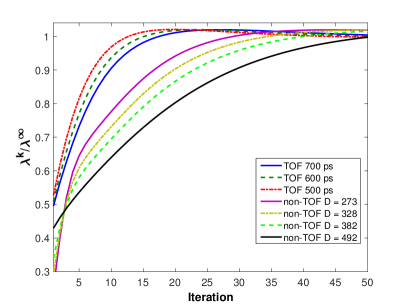
(a) Activity value

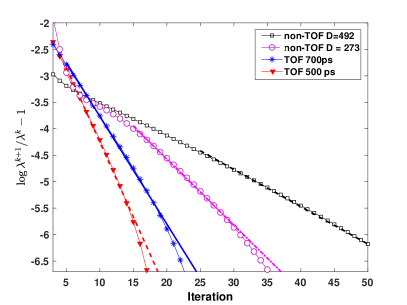
(b) Linear-log plot of equation 10

Figure 1: Convergence of circles with contrast $\beta=2.4$ and diameter $d=22\,mm$ for different background diameters and CTR.

1 shows the results of the simulations: plots of activity values for representative circles (a), together with the linear-log plots of equation 10 (b). For TOF only $D=410\,mm$ curves are shown as they were perfectly superimposed for all diameters. Plots of $\alpha_{j}$ as a function of background diameter, contrast and object size are shown in supplementary figure 1. For $\log\alpha_{j}\apprge 0.30$, model fitting was difficult due to the very high convergence speed. This prevented us to investigate the model for higher contrasts and lower CTRs. Equation 7 was found able to correctly describe the convergence rate for all the diameters and contrasts investigated, with $\gamma=0.59\pm 0.08$, both for TOF and non-TOF recons. The discrepancy between predicted and fitted $\gamma$ is acceptable considering the high number of assumptions on $\alpha_{j}$ and $\lambda_{j}$ trends along a LOR. As to TOF, simulations confirmed the independence of the convergence speed from the background diameter.

3.3 Noise properties

3.3.1 Methods

A uniform phantom of $410\,mm$ diameter was simulated and reconstructed over a $512\,mm$ FOV using $2\,mm$ pixels. Images were forward projected without and with TOF at CTR of $650,\,400,\,300\,,80\,ps$ FWHM that correspond to a $D_{eff}=104,\,64,\,48\,,13\,mm$. Attenuation, random and scatter were not simulated. A Poisson process was simulated to achieve 12 independent noise realizations of the noiseless sinogram. An identical total number of counts was simulated at different CTRs. Images were reconstructed using MLEM without OS acceleration over 1000 iterations.

To quantify image noise, activity was sampled in 148 close but not contiguous pixels at the image center. Noise was computed as the average over the 148 pixels of the standard deviation among the 12 realizations. A linear fit of noise vs the number of iterations was performed by using only the first 5 iterations. The relation between the fit slope and background diameter was compared to that predicted in equation 19. The ratio between TOF and non-TOF noise at convergence was compared to the predictions made in reference [1].

As previously stated, the convergence of each noise frequency $f$ should follow equation 6 with $\beta=1$ and $d=\nicefrac{{1}}{{f}}$. However, a linear-log fit cannot be performed, since noise in a uniform disk simultaneously involves all possible frequencies. Therefore, we analyzed the noise power spectrum at representative number of iterations, and noise as a function of iterations on post-filtered images.

3.3.2 Results

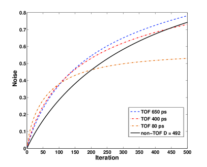
(a) Plots of noise as a function of the iterations on unfiltered images. Selected CTR shown for clarity

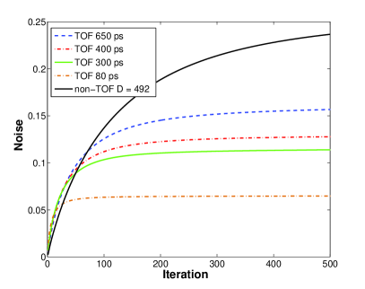
(b) Plot of noise as a function of iterations for images post-smoothed with a $4.5\,mm$ Gaussian filter

Figure 2: Noise as a function of iterations

In 2a noise is shown as a function of iterations for the first $500$ iterations. In the first iterations, shown in supplementary figure 2, it can be properly described by the linear model within a $25\%$ error up to $79$ iterations for non-TOF, to $27$ iterations for TOF with $650\,ps$ CTR, $16$ iterations for $400\,ps$ and $8$ iterations for $80\,ps$. The slopes follow the $\nicefrac{{1}}{{\sqrt{D_{eff}}}}$ trend as predicted in section 2.3.2. With TOF at $650$ or $400\,ps$ is higher than in non-TOF up to $\approx 500$ iterations. Up to $1000$ iterations MLEM has not reached convergence yet. Ratios between TOF and non-TOF noise at convergence ($6000$ iterations) corresponds to predictions in reference [1] (results not shown). In supplementary figure 3 we show the noise power spectrum at different number of iterations for non-TOF and TOF with $400\,ps$ CTR. At low iterations, the noise power spectrum resembles the $\nicefrac{{1}}{{r}}$ trend, while at convergence it approximates the ramp. This was expected under the considerations introduced in (2.3.2). The low frequency noise power is lower with TOF than without it. As to higher frequencies, without TOF, they are still far from convergence at $1000$ iterations, while with TOF the usual shape of the ramp filter can be appreciated. In 2b we show noise as a function of iterations, on images post-filtered with a $4.5\,mm\,FWHM$ Gaussian kernel. Noise converges much quicker than without any smoothing, nonetheless, TOF reconstructions with CTR of $400\,ps$ still have noise higher than non-TOF up to $\approx 60$ iterations.

4 Phantom measurements

4.1 Methods

4.1.1 Phantom preparation and acquisition

Two $22\,cm$ diameter Derenzo phantoms were filled with ${}^{18}F-FDG$. The first phantom has the cold insert and was filled with $15.5\;kBq/cc$ of activity, calibrated at the time of the first scan. In the uniform region, six cold spheres of $8,\,11,\,14,\,17,\,24$ and $30\,mm$ diameters were positioned. The second phantom has the hot insert and was filled with $15.4\;kBq/cc$ of activity in the background region. It also featured 6 hot spheres of $7,\,12,\,15,\,16,\,19$ and $24\,mm$ diameter, filled with a $4.48:1$ activity ratio vs the background. The phantoms were acquired both individually (“Single” configuration) and side by side (“Double” configuration), to simulate different object dimensions. In the double configuration, the active area has a major axis of about $44\,cm$ and a minor axis of $22\,cm$, which is close to the dimension of a typical patient.

To investigate the effect of TOF at different CTRs, the phantoms were scanned in two different PET tomographs: a General Electrics Medical Systems SIGNA PET/MR, with $400\,ps$ CTR and a GEMS Discovery D690 with $650\,ps$ CTR. To better investigate the random coincidences effect, the double configuration was scanned twice in the SIGNA: the first time immediately after preparation with a true to random coincidences ratio $\approx 1$ (“HCR” high count rate configuration), and the second time $2\,h\,21\,min$ later, with a true to random coincidences ratio $\approx 5:1$ (“LCR” low count rate configuration). Each configuration was acquired for 10 minutes in list mode. Data were then unlisted into 5 frames of 2 minutes to simulate multiple noise realizations.

4.1.2 Image reconstruction

To analyze early convergence, few iterations of MLEM without OS acceleration were performed (SIGNA: TOF: 20, non-TOF: 40. D690: TOF: 30, non-TOF: 60). To study the convergence of high frequencies and noise with and without TOF, a second reconstruction was performed with a full 3D-OSEM algorithm using 16 subsets and 80 iterations (1280 updates or MLEM equivalent iterations). Images were reconstructed using a $256\times 256$ image matrix, on the maximum scanner FOV($70\,cm$ D690; $60\,cm$ SIGNA) and were post-filtered with a $4.5\,mm\;FWHM$ in-plane Gaussian filter.

4.1.3 Image analysis

To study the signal convergence rate, the activity measured in the central pixel of each sphere was fitted to equation 10 . To quantify image noise, activity was sampled in 320 close but not contiguous pixels of both phantoms. Noise was computed as the average over the 320 pixels of the standard deviation among the 5 noise realizations.

4.1.4 Estimation of random and scatter coincidences

In these phantom experiments, high fractions of random and scatter coincidences are present. To fit equation 6, we need to estimate the ratio between true counts and random and scattered counts in each sinogram bin. We thus forward projected the reconstructed image and multiplied the resulting sinogram by the attenuation and the normalization sinogram. We then used scatter and random coincidence sinograms to compute count ratios.

4.2 Results

4.2.1 Sphere convergence

The convergence of a representative sphere, together with its linear-log plots are shown in 3. The convergence was well described by the the linear fit. Nonetheless, since spheres are not in the background center and due to the presence of scatter and random coincidences, the coefficient $\alpha_{j}$ can not be simply described in terms of contrast and dimension like in equation 7, but the whole equation 6 must be used. In 1 we show fitted values of $\alpha_{j}$ for the $15\,mm$ sphere for the different configurations in the two PET scanners.

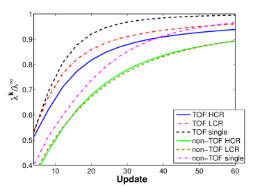
(a) Convergence of activity

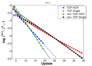
(b) Linear-log plots of equation 10. Only 4 acquisitions shown for clarity

Figure 3: Convergence analysis of the $15\,mm$ sphere acquired on the SIGNA

Acquisition	non-TOF D690	non-TOF SIGNA	TOF D690	TOF SIGNA
Single	0.099	0.085	0.115	0.171
Double LCR	0.067	0.068	0.136	0.143
Double HCR		0.077		0.131

Table 1: Values of $\alpha_{j}$ for the $15\,mm$ sphere

Without TOF, D690 and the SIGNA scanner values are similar. When TOF is introduced, SIGNA has a higher convergence speed, thanks to its better CTR.

4.2.2 Noise proprieties

In supplementary figure 4 we show the noise trends as a function of iterations for D690 acquisitions. In figure 4 we show the same trends for the SIGNA scanner acquisitions. Noise is higher with TOF than without it up to $200$ updates in the HCR configuration and up to $120$ updates in the Single and the LCR configurations. Curves are more detached than those obtained on the D690 scanner, because of the lower CTR.

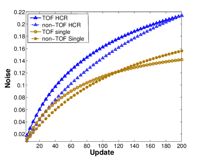
(a) Noise in the first iterations. LCR not shown for clarity

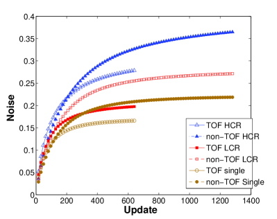
(b) Noise trend at all iterations reconstructed

Figure 4: Noise for TOF and non-TOF measured in the phantoms acquired in the SIGNA scanner.

At $1280$ updates noise in non-TOF has not converged yet. In table 2 we report the noise increase from non-TOF to TOF reconstructions at 48 updates, a common clinical setting. In the single configuration, in the D690 scanner almost no differences are observed, as the CTR is not significantly smaller than the phantom diameter. On the SIGNA scanner the increase is larger than in the D690 scanner.

	SIGNA	D690
	[%]	[%]
Single	+16.9	+4.2
Double LCR	+13	+10.0
Double HCR	+25.6

Table 2: Noise increase at 48 updates between TOF and non-TOF reconstructions

4.2.3 Impact of scatter and random coincidences

Results in 2 show that the noise increase from non-TOF to TOF is higher in HCR configuration than in the LCR one. This is in accordance with what obtained in 2.4. In supplementary figure 5 we show, for the LCR SIGNA acquisitions, the estimated trues, scatter and random coincidences along the TOF dimension for two orthogonal projections along the major and the minor axis and of the phantom. As expected, the scatter distribution follows the trues coincidences distribution, thereby limiting the improvements achievable by TOF.

5 Proposed early stopping criteria

Currently, in non-TOF reconstructions, it is customary to estimate the optimal trade-off between signal recovery and noise on image quality phantoms. Such phantoms are generally small in diameter compared to patients and signal recovery is measured in a relatively high contrast setup (e.g.: $10:1$). As we have shown, if the stopping criteria are optimized on a high signal contrast and with a small diameter background, when they are applied to patient areas like the abdomen, characterized by a large diameter and by the presence of high uptake organs in the background, a serious risk of signal under-recovery may appear. Nonetheless, the widespread adoption of early stopping in the last decades has shown that such criteria are effective enough to allow a robust diagnosis.

We here propose a stopping rule definition method for TOF to maximally exploit TOF potentialities for a given combination of PET scanner, injected dose and acquisition duration. First, a non-TOF reconstruction stopping criteria $N_{it}$ has to be established according to the current standard, using an image quality phantom, possibly with a lower contrast (e.g $4:1$). Then, the optimal stopping criteria for TOF can be obtained as $N_{TOF}=N_{it}\times\nicefrac{{D_{eff}}}{{20\,cm}}$ . On $20\,cm$ objects, this stopping criteria would provide the noise reduction theoretically expected for TOF [1] and a signal recovery comparable to that achievable with non-TOF reconstruction. For objects smaller than $20\,cm$, a slight under-recovery with respect to non-TOF reconstructions would be present, but signal recovery in small objects is generally not an issue. On objects larger than $20\,cm$ this criteria maintains the signal recovery determined on the image quality phantom and still provide a noise reduction, even if by a factor smaller than $\sqrt{\nicefrac{{D_{eff}}}{{D}}}$.

The effects of this criteria can be qualitatively appreciated by analyzing results obtained on the SIGNA scanner. On the Single configuration of the hot phantom, we estimated 48 updates to be a reasonable stopping criteria for non-TOF reconstruction. According to the proposed criteria, we selected 16 updates for TOF reconstruction. In figure 5, two slices of the phantom obtained with 48 updates of non-TOF and 16 updates of TOF are shown. In the slice containing hot spheres, detectability is visually similar with TOF, while noise is markedly reduced. In the slice with the Jaszczak insert, TOF provides a visually better image quality, despite the lower number of iterations.

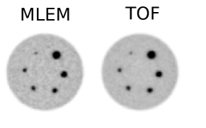
(a) First slice

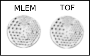
(b) Second slice

Figure 5: Two slices of the phantom in the single configurations, reconstructed using the proposed stopping criteria

In figure 6, images of the Double configuration phantom obtained with the same reconstruction strategies are shown. In the slice containing the hot spheres and the cold Jaszczak insert, TOF shows slightly better hot sphere contrast at much lower noise, and a higher cold contrast. In the slice containing the cold spheres and the hot Jaszczak insert, TOF markedly improves image quality respect to non-TOF, that at 48 updates, is not able to recover details at the FOV center yet.

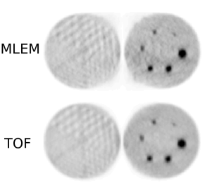
(a) First slice

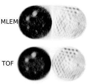
(b) Second slice

Figure 6: Double phantom reconstructed with the proposed criteria

6 Discussion

In this paper we revised PET MLEM convergence properties, with the aim to investigate TOF influence on signal recovery and noise amplification on early stopped reconstructions, as these are still the most widely used in clinical routine. In the theoretical analysis it was found that signal convergence speed increases with signal contrast and dimension, while it decreases with background diameter. TOF, in an ideal condition without random and scatter coincidences, is able to eliminate the dependence of signal convergence on the background diameter, thus making the use of early stopped reconstructions more robust to variations in patient size and background composition. Random and scatter coincidences generally decrease the convergence speed. Importantly, TOF is able to significantly reduce the impact of random coincidences on convergence; scatter coincidences, instead, increase with patient size and, due to their distribution, their impact is not greatly reduced by TOF. All these findings were theoretically proved and confirmed by simulations and phantom experiments.

As to noise behavior with iterations, higher frequencies converge more slowly than lower ones, thanks to the low-pass effect of the backprojection forward-projection sequence, base of the MLEM algorithm. TOF reduces this low-pass filtering effect, thus making noise convergence faster. While at convergence TOF reduces noise respect to non-TOF by a factor $\sqrt{\frac{D_{eff}}{D}}$, if matched iterations are used in early iterations TOF actually increases noise by the inverse of this factor, thus resulting in sub-optimal exploitation of TOF gains. In simulations, we found that TOF with $400\,ps$ CTR had noise higher than non-TOF up to$\approx 60$ iterations. In phantom experiments, this limit is shifted to higher iteration values, because of the influence of random and scattered coincidences on the convergence speed. On the SIGNA scanner, the crossing point was obtained at $120$ iterations for the Single configuration ($22\,cm$ axis) and at $200$ iterations for the Double configuration ($44\,cm$ major axis). In the HCR configuration, characterized by a high number of random and scattered events, at $50$ iterations noise was increased by TOF of $25\%$. For this reason, until regularization algorithms become routine in clinical applications, we suggest a criteria to properly reduce the iteration number when using TOF, to optimize TOF benefits in early-stopped MLEM. Stopping at $\nicefrac{{D_{eff}}}{{20\,cm}}$ of the iterations used without TOF, provides matched signal recovery and noise reduction for small objects, and greatly improves recovery for large objects.

The novelty of this work lies in the theoretical derivation of the convergence of signal and noise in MLEM, with and without TOF. In non-TOF systems, using a fixed number of iterations results in approximately constant levels of noise for all body shapes and regions, due to the proprieties highlighted in 2.3. The signal recovery instead is strongly influenced by all these factors, therefore the recovery factors measured in phantoms might severely overestimate the recovery factors for low contrast objects in large backgrounds (typically liver lesions, especially in obese patients). The proposed criteria instead, guarantees that when TOF is used approximately the same contrast recovery measured on the phantom used to choose the stopping criteria is obtained in all imaging conditions, achieving therefore both a noise reduction and also a more robust quantification.

7 Conclusion

The convergence proprieties of signal and noise in MLEM were revised, taking into account the effect of TOF. Previous empirical findings of increased convergence speed both of signal and noise were confirmed. Finally, we introduced a way to determine using phantoms a stopping criterion that guarantees background-independent levels of contrast recovery, that can be determined a priori on phantoms.

References

- [1] K. Vunckx, Lin Zhou, S. Matej, M. Defrise, and J. Nuyts. Fisher Information-Based Evaluation of Image Quality for Time-of-Flight PET. IEEE Transactions on Medical Imaging, 29(2):311–321, feb 2010.
- [2] L. A. Shepp and Y. Vardi. Maximum Likelihood Reconstruction for Emission Tomography. IEEE Transactions on Medical Imaging, 1(2):113–122, oct 1982.
- [3] H. Malcolm Hudson and Richard S. Larkin. Accelerated Image Reconstruction Using Ordered Subsets of Projection Data. IEEE Transactions on Medical Imaging, 13(4):601–609, 1994.
- [4] Valentino Bettinardi, L Presotto, E Rapisarda, M Picchio, L Gianolli, and M C Gilardi. Physical Performance of the new hybrid PET/CT Discovery-690. Med Phys, 38(10):5394–5411, 2011.
- [5] Maurizio Conti. Focus on time-of-flight PET: the benefits of improved time resolution. European Journal of Nuclear Medicine and Molecular Imaging, 38(6):1147–1157, jun 2011.
- [6] Maurizio Conti, Lars Eriksson, and Victor Westerwoudt. Estimating Image Quality for Future Generations of TOF PET Scanners. IEEE Transactions on Nuclear Science, 60(1):87–94, feb 2013.
- [7] J. S. Karp, S. Surti, M. E. Daube-Witherspoon, and G. Muehllehner. Benefit of Time-of-Flight in PET: Experimental and Clinical Results. Journal of Nuclear Medicine, 49(3):462–470, mar 2008.
- [8] Joyce J van Sluis, Johan de Jong, Jenny Schaar, Walter Noordzij, Paul van Snick, Rudi Dierckx, Ronald Borra, Antoon Willemsen, and Ronald Boellaard. Performance characteristics of the digital Biograph Vision PET/CT system. Journal of Nuclear Medicine, page jnumed.118.215418, jan 2019.
- [9] H H Barrett, D W Wilson, and B M W Tsui. Noise properties of the EM algorithm. I. Theory. Physics in Medicine and Biology, 39(5):833–846, may 1994.
- [10] Johan Nuyts. Unconstrained image reconstruction with resolution modelling does not have a unique solution. EJNMMI Physics, 1(1):98, dec 2014.
- [11] K. Lange. Convergence of EM image reconstruction algorithms with Gibbs smoothing. IEEE Transactions on Medical Imaging, 9(4):439–446, 1990.
- [12] Charles Watson. Extension of Single Scatter Simulation to Scatter Correction of Time-of-Flight PET. IEEE Transactions on Nuclear Science, 54(5):1679–1686, oct 2007.
- [13] Yusheng Li. Noise propagation for iterative penalized-likelihood image reconstruction based on Fisher information. Physics in Medicine and Biology, 56(4):1083–1103, feb 2011.
- [14] Ravindra M. Manjeshwar, Steven G. Ross, Maria Iatrou, Timothy W. Deller, and Charles W. Stearns. Fully 3D PET iterative reconstruction using distance-driven projectors and native scanner geometry. IEEE Nuclear Science Symposium Conference Record, 5:2804–2807, 2007.