Realization of analytic moduli
for parabolic Dulac germs

Abstract.

In a previous paper [7] we have determined analytic invariants, that is, moduli of analytic classification, for parabolic generalized Dulac germs. This class contains parabolic Dulac (almost regular) germs, that appear as first return maps of hyperbolic polycycles. Here we solve the problem of realization of these moduli.

Acknowledgement. This research was supported by the Croatian Unity Through Knowledge Fund (UKF) My first collaboration grant project no. 16, by the Croatian Science Foundation (HRZZ) grants UIP-2017-05-1020 and PZS-2019-02-3055 from Research Cooperability funded by the European Social Fund, and by the EIPHI Graduate School (contract ANR-17-EURE-0002). The UKF grant fully supported the $6$-month stay of ² at Université de Bourgogne in 2018.

1. Introduction and main definitions

Dulac germs, called almost regular germs in [2], appear as first return maps on transversals to hyperbolic polycycles in planar analytic vector fields, see e.g. [2] or [10]. From the viewpoint of cyclicity of planar vector fields, the most interesting case is the case of Dulac germs tangent to the identity. Using notation similar as in the case of $1$-dimensional analytic diffeomorphisms, we call such germs which are not roots of the identity parabolic Dulac germs.

In [7], we have described the Ecalle-Voronin-like moduli of analytic classification for a bigger class of parabolic generalized Dulac germs. Parabolic generalized Dulac germs defined in [7] are a class of germs, including parabolic Dulac germs, that admit a particular type of transserial power-logarithmic asymptotic expansion, called the generalized Dulac asymptotic expansion. They are, like Dulac germs, defined on a standard quadratic domain: a universal covering of $\mathbb{C}$ punctured at the origin with a prescribed decreasing radius as the absolute value of the argument increases. Their moduli are given as a doubly infinite sequence of pairs of germs of diffeomorphisms fixing the origin, having a symmetry property with respect to the positive real axis and a rate of decrease of radii of convergence adapted to the standard quadratic domain of definition. Similarly as in the well-known case of analytic parabolic germs treated in [12], it was shown in [7] and [8] that the formal class of a generalized Dulac germ is described by three parameters, but the normalizing change diverges and defines analytic functions only on overlapping attracting and repelling sector-like domains called petals. There are countably many petals filling the standard quadratic domain and the comparison of normalizing changes on their intersections, together with the formal class of the germ, gives its modulus of analytic classification.

As a continuation of [7], in this paper we describe the space of moduli, that is, we solve the problem of realization of moduli of analytic classification in the class of parabolic generalized Dulac germs. For each formal class and a double sequence of germs of diffeomorphisms fixing the origin with controlled radii of convergence, we construct an analytic germ defined on a standard quadratic domain realizing them.

However, on a big standard quadratic domain we did not succeed in attributing a unique power-logarithmic transserial asymptotic expansion to the constructed germ. Transseries are indexed by ordinals, which can either be successor ordinals or limit ordinals. The definition of a transserial asymptotic expansion of a certain type is dependent on the choice of the summation method at limit ordinal steps. This choice is called a section function in [9]. To ensure uniqueness of the asymptotic expansion, we should be able to make a canonical choice of the section function. See [9] for more details on the problem of well-defined transserial asymptotic expansions and the notion of section functions.

Moreover, we prove that, on a smaller linear domain, there exists a parabolic generalized Dulac germ of a given formal type which realizes the given sequence of diffeomorphisms as its analytic moduli. On this smaller domain we are able to choose a canonical method of summation on limit ordinal steps, a Gevrey-type sum, corresponding to the definition of the generalized Dulac asymptotic expansion requested in the definition of generalized Dulac germs.

In both constructions we use a Cauchy-Heine integral construction as in e.g. [5], motivated by the realization of analytic moduli for saddle nodes in [11]. The advantage of the Cauchy-Heine construction over the standard use of uniformization method, as in [12], is that Cauchy-Heine integrals provide the control of power-logarithmic asymptotic expansions.

Let us first recall briefly main definitions and results from [7].

1.1. Main definitions

Recall from Ilyashenko [2] the definition of almost regular germs. We call them Dulac germs in [7] and also here. They are defined on a standard quadratic domain $\mathcal{R}_{C}$. It is a subset of the Riemann surface of the logarithm, in the logarithmic chart $\zeta=-\log z$ given by:

(1.1) $$\varphi\big{(}\mathbb{C}^{+}\setminus\overline{K}(0,R)\big{)},\ \varphi(\zeta)=\zeta+C(\zeta+1)^{\frac{1}{2}},\ C>0,\,R>0.$$

Here, $\mathbb{C}^{+}=\{\zeta\in\mathbb{C}:\ \text{Re}(\zeta)>0\}$ and $\overline{K}(0,R)=\{\zeta\in\mathbb{C}:|\zeta|\leq R\}.$ See Figure 1.1. In the sequel, we switch between the two variables, the $z$-variable and the $\zeta$-variable, as needed. By abuse, we use the same name standard quadratic domain for the domain in the $\zeta$-variable defined by (1.1) and for its preimage by $\zeta=-\log z$ in the universal covering of $\mathbb{C}^{*}$. In $z$-variable we use the notation $\mathcal{R}_{C}$, while we use the notation $\widetilde{\mathcal{R}}_{C}$ for its image by $\zeta=-\log z$ in the $\zeta$-variable.

Definition 1.1 (Definition 2.1. in [7], adapted from [2], [10]).

We say that a germ $f$ is a Dulac germ if it is

1. holomorphic and bounded on some standard quadratic domain $\mathcal{R}_{C}$ and real on $\{z\in\mathcal{R}_{C}:\ \mathrm{Arg}(z)=0\}$,

2. admits in $\mathcal{R}_{C}$ a Dulac asymptotic expansion

   (1.2) $$\widehat{f}(z)=\sum_{i=1}^{\infty}z^{\lambda_{i}}P_{i}(-\log z),\ c>0,\ z\to 0,$$

   where $\lambda_{i}\geq 1$, $i\in\mathbb{N}$, are strictly positive, finitely generated and strictly increasing to $+\infty$ and $P_{i}$ is a sequence of polynomials with real coefficients, and $P_{1}\equiv A$, $A>0$.

Moreover, if a Dulac germ is tangent to the identity, i.e,

$$f(z)=z+o(z),\ z\in\mathcal{R}_{C},$$

and if $f^{\circ q}\neq\mathrm{id}$, $q\in\mathbb{N}$, we call it a parabolic Dulac germ.

By a germ on a standard quadratic domain [2], we mean an equivalence class of functions that coincide on some standard quadratic domain (for arbitrarily big $R>0$ and $C>0$).

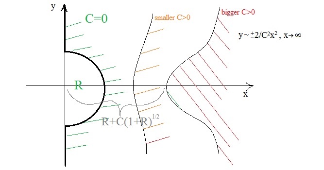
Figure 1.1. Several standard quadratic domains $\widetilde{\mathcal{R}}_{C}$, $C>0$, in the logarithmic chart.

The radii of the standard quadratic domain in $z$-variable tend to zero with an exponential speed as we increase the level of the Riemann surface. If by $\theta\in\big{[}(k-1)\pi,(k+1)\pi\big{)}$ we denote the arguments of the $k$-th level of the surface $\mathcal{R}_{C}$, $k\in\mathbb{Z},$ and by $\theta_{k}:=k\pi$, $k\in\mathbb{Z},$ then the maximal radii $r(\theta_{k})$ by levels $k\in\mathbb{Z}$ decrease at most at the rate:

$$Ke^{-D\sqrt{\frac{|k|\pi}{2}}},\ |k|\to\infty,\ \text{for some }D>0,\ K>0.$$

In [7, Definition 2.3], a larger parabolic generalized Dulac class is introduced. It contains parabolic Dulac germs. We repeat the definition of parabolic generalized Dulac germs in Definition 1.4 below. The Dulac asymptotic expansion requested in Definition 1.1 of Dulac germs is substituted by a particular transserial power-logarithmic asymptotic expansion.

In this paper, we give realization results for any given sequence of moduli satisfying some uniform bound in the parabolic generalized Dulac class, but for parabolic generalized Dulac germs defined on a smaller domain that we call a standard linear domain. Due to technical reasons in Cauchy-Heine construction, on standard quadratic domain we get realization results by germs for which we are unable to prove unicity of the transserial asymptotic expansion after the first three terms. To be able to define the unique transserial asymptotic expansion of a germ of a certain type, we should be able to prescribe a canonical way of summation, or section function [9], at limit ordinal steps. In the linear case, the estimates of the Cauchy-Heine integrals give us sufficiently good Gevrey-like bounds, and thus a canonical way to attribute the sum, at limit ordinal steps. This canonical choice is the one defining parabolic generalized Dulac germs and expansions, see Definitions 1.3 and 1.4 below. On the other hand, the bounds in our construction on standard quadratic domains are weaker.

It is important to note that the germ obtained by Cauchy-Heine construction on a linear domain is not the restriction of the germ constructed on a bigger quadratic domain, since we apply Cauchy-Heine integrals along different lines of integration, see (LABEL:eg:lint) under condition (3.9) for standard quadratic domains or (3.10) for standard linear domains. For details, see Remarks 3.6 and 5.2.

By [3, 10], a standard linear domain is not sufficiently large to apply Phragmen-Lindelöf and get injectivity of the mapping $f\mapsto\widehat{f}$, where $\widehat{f}$ is the generalized Dulac asymptotic expansion of $f$.

Definition 1.2.

A standard linear domain $\widetilde{\mathcal{R}}_{a,b}$, $a>0,\ b\geq 0,$ in the logarithmic chart is a subset of $\mathbb{C}_{+}$ given by:

$$\widetilde{\mathcal{R}}_{a,b}:=\Big{\{}\zeta\in\mathbb{C}_{+}:\ b-a\mathrm{Re}(\zeta)<\mathrm{Im}(\zeta)<-b+a\mathrm{Re}(\zeta),\ \mathrm{Re}(\zeta)>\frac{b}{a}\Big{\}}.$$

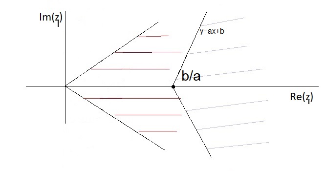
Figure 1.2. Several standard linear domains $\widetilde{\mathcal{R}}_{a,b}$, $a>0,\ b\geq 0$, in the logarithmic chart.

Analogously, by $\mathcal{R}_{a,b}$ we denote the image by $z=e^{-\zeta}$ of $\widetilde{\mathcal{R}}_{a,b}$. It is a subset of the Riemann surface of the logarithm.

We recall from [7] the definition of the parabolic generalized Dulac class. We will call an $\boldsymbol{\ell}$-cusp an open cusp that is the image of an open sector $V$ of positive opening at $0$ by the change of variables $\boldsymbol{\ell}=-\frac{1}{\log z}$, and we will denote it by $S=\boldsymbol{\ell}(V)$. See Figure 1.3. Any open $\boldsymbol{\ell}$-cusp $\boldsymbol{\ell}(V^{\prime})\subset S$, where $V^{\prime}\subset V$ is a proper subsector, will be called a proper $\boldsymbol{\ell}$-subcusp of $S$.

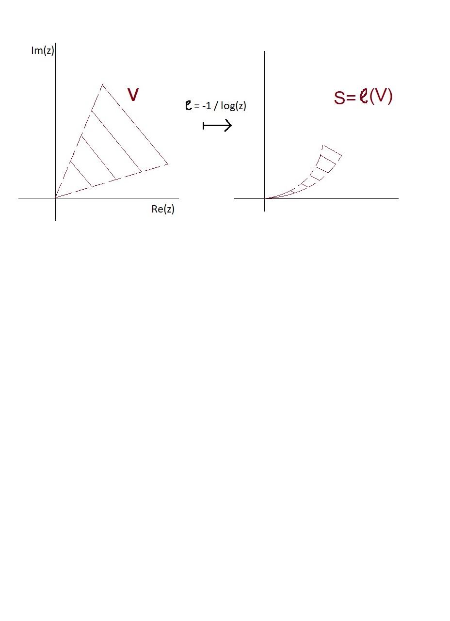
Figure 1.3. $\boldsymbol{\ell}$-cusp.

Definition 1.3 ($\log$-Gevrey asymptotic expansions on $\boldsymbol{\ell}$-cusps, Definition 4.1 in [7]).

Let $F$ be a germ analytic on an $\boldsymbol{\ell}$-cusp $S=\boldsymbol{\ell}(V)$. We say that $F$ admits $\widehat{F}(\boldsymbol{\ell})=\sum_{k=0}^{\infty}a_{k}\boldsymbol{\ell}^{k}$, $a_{k}\in\mathbb{C}$, as its $\log$-Gevrey asymptotic expansion of order $m>0$ if, for every proper $\boldsymbol{\ell}$-subcusp $S^{\prime}=\boldsymbol{\ell}(V^{\prime})\subset S$, $V^{\prime}\subset V,$ there exists a constant $C_{S^{\prime}}>0$ such that, for every $n\in\mathbb{N}$, $n\geq 2,$ it holds that:

$$|F(\boldsymbol{\ell})-\sum_{k=0}^{n-1}a_{k}\boldsymbol{\ell}^{k}|\leq C_{S^{\prime}}\cdot m^{-n}\cdot\log^{n}n\cdot e^{-\frac{n}{\log n}}|\boldsymbol{\ell}|^{n},\ \boldsymbol{\ell}\in S^{\prime}.$$

For more details on properties of $\log$-Gevrey classes and for the proof of their closedness to algebraic operations $+,\cdot$ and to differentiation, see [7, Section 4]. We state here just the following variation of the Watson’s lemma for $\log$-Gevrey expansions, that will be immediately important for the definition and the uniqueness of generalized Dulac expansions. If $\widehat{F}(\boldsymbol{\ell})$ is the $\log$-Gevrey asymptotic expansion of order $m>0$ of a function $F$ analytic on $\boldsymbol{\ell}$-cusp $S=\boldsymbol{\ell}(V)$, where $V$ is a sector of opening strictly bigger than $\frac{\pi}{m}$, then $F$ is the unique analytic function on $S$ that admits $\widehat{F}(\boldsymbol{\ell})$ as its $\log$-Gevrey asymptotic expansion of order $m$. The proof can be found in [7, Section 4, Corollary 4.4].

We prove in [7, Proposition 2.2] that every parabolic germ $f$ on $\mathcal{R}_{C}$ (resp. $\mathcal{R}_{a,b}$) that satisfies the uniform asymptotics:

$$\big{|}f(z)-(z-az^{\alpha}\boldsymbol{\ell}^{m})\big{|}\leq c|z^{\alpha}\boldsymbol{\ell}^{m+1}|,\ z\in\mathcal{R}_{C}\text{ (resp. $\mathcal{R}_{a,b}$)},$$

$$\alpha>1,\ m\in\mathbb{Z},\ a\neq 0,\ c>0,$$

has a local flower-like dynamics at the origin. That is, $\mathcal{R}_{C}$ (resp. $\mathcal{R}_{a,b}$) is a union of countably many overlapping invariant attracting and repelling petals $V_{j}^{+}$ resp. $V_{j}^{-}$, $j\in\mathbb{Z}$, centered at directions $a^{-\frac{1}{\alpha-1}}$ resp. $(-a)^{-\frac{1}{\alpha-1}}$, and of opening $\frac{2\pi}{\alpha-1}$.

The dynamics in the $\zeta$-variable on a standard quadratic domain $\widetilde{\mathcal{R}}_{C}$ is shown on Figure 1.4. The sectors of opening $\theta>0$ in the $z$-variable become horizontal strips of width $\theta>0$ in the $\zeta$-variable. Analogously, the images of petals of opening $\frac{2\pi}{\alpha-1}$ in the $z$-variable are open sets tangentially approaching strips of width $\frac{2\pi}{\alpha-1}$, as $\mathrm{Im}(\zeta)\to+\infty$, in the $\zeta$-variable. We denote them in the $\zeta$-variable by $\tilde{V}_{j}^{+}$ and $\tilde{V}_{j}^{-}$, $j\in\mathbb{Z}$, see Figure 1.4. By abuse, in the $\zeta$-variable, we also call them petals.

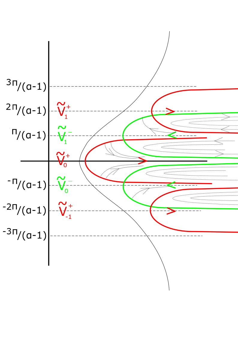
Figure 1.4. The outline of the dynamics of a generalized Dulac germ on petals $\tilde{V}_{j}^{\pm}$, $j\in\mathbb{Z}$, along a standard quadratic domain $\widetilde{\mathcal{R}}_{C}$ in the logarithmic chart, case $a>0$ in (1.3), [7, Figure 3.1].

Definition 1.4 (Parabolic generalized Dulac germs, Definition 2.3 in [7]).

We say that a parabolic germ $f$, analytic on a standard quadratic domain $\mathcal{R}_{C}$ $($or: standard linear domain $\mathcal{R}_{a,b})$, that maps $\{\mathrm{arg}(z)=0\}\cap\mathcal{R}_{C}$ $($resp. $\{\mathrm{arg}(z)=0\}\cap\mathcal{R}_{a,b})$ to itself, satisfying

(1.3) $$|f(z)-z+az^{\alpha}\boldsymbol{\ell}^{m}|\leq c|z^{\alpha}\boldsymbol{\ell}^{m+1}|,\ a\neq 0,\ \alpha>1, \ m\in\mathbb{Z},\ c>0,$$

$$z\in\mathcal{R}_{C}\text{, resp. $z\in\mathcal{R}_{a,b}$},$$

is a parabolic generalized Dulac germ if, on its every invariant petal $V_{j}^{\pm},\ j\in\mathbb{Z}$, of opening $\frac{2\pi}{\alpha-1}$, it admits an asymptotic expansion of the form:

$$f(z)=z+\sum_{i=1}^{n}z^{\alpha_{i}}R_{i}^{j,\pm}(\boldsymbol{\ell})+o(z^{\alpha_{n}+\delta_{n}}),\ \delta_{n}>0,$$

for every $n\in\mathbb{N}$, as $z\to 0$ on $V_{j}^{\pm}$. Here, $\alpha_{1}=\alpha$, $\alpha_{i}>1$ are strictly increasing to $+\infty$ and finitely generated, and $R_{i}^{j,\pm}(\boldsymbol{\ell})$ are analytic functions on open cusps $\boldsymbol{\ell}(V_{j}^{\pm})$ which admit common $\log$-Gevrey asymptotic expansions $\hat{R}_{i}(\boldsymbol{\ell})$ of order strictly bigger than $\frac{\alpha-1}{2}$, as $\boldsymbol{\ell}\to 0$:

$$\hat{R}_{i}(\boldsymbol{\ell})=\sum_{k=N_{i}}^{\infty}a_{k}^{i}\boldsymbol{\ell}^{k},\ a_{k}^{i}\in\mathbb{R},\ N_{i}\in\mathbb{Z}.$$

We then say that the transseries $\widehat{f}$ given by:

(1.4) $$\widehat{f}(z):=z+\sum_{i=1}^{\infty}z^{\alpha_{i}}\widehat{R}_{i}(\boldsymbol{\ell})$$

is the unique generalized Dulac asymptotic expansion of $f$. Such $\widehat{f}$ is called a parabolic generalized Dulac series.

Note that all coeficients of the expansion are real, due to the invariance of $\mathbb{R}_{+}$ under $f$.

Moreover, we assume in the sequel that $a>0$ in (1.3). That is, that $\mathbb{R}_{+}\cap\mathcal{R}_{C}$ is an attracting direction. If $a<0$, we consider the inverse generalized Dulac germ $f^{-1}$. Indeed, it was proven in [7, Proposition 8.2] that parabolic generalized Dulac germs form a group under composition.

A generalized Dulac asymptotic expansion is an asymptotic expansion in the formal class of transseries $\widehat{\mathcal{L}}(\mathbb{R})$. The class of power-logarithmic transseries $\widehat{\mathcal{L}}(\mathbb{R})$ was first introduced in [8], as the class of transseries of the form:

$$\widehat{f}(z)=\sum_{i=1}^{\infty}\sum_{m=N_{i}}^{\infty}a_{i,m}z^{\alpha_{i}}\boldsymbol{\ell}^{m},\ a_{i,m}\in\mathbb{R},$$

where $\alpha_{i}>0$ are finitely generated and strictly increasing to $+\infty$, and $N_{i}\in\mathbb{Z}$, $i\in\mathbb{N}$. Here, $\boldsymbol{\ell}=\frac{1}{-\log z}$. As discussed in [9], an asymptotic expansion of a germ in $\widehat{\mathcal{L}}(\mathbb{R})$ is in general not well-defined, nor unique. The generalized Dulac expansion is a sectional asymptotic expansion (see [9] for precise definition of sections) that becomes unique after a canonical choice of section functions (the summation method) at limit ordinal steps - here, the $\log$-Gevrey sums of a certain order.

The parabolic Dulac (almost regular in [2]) germs from Definition 1.1 are trivially parabolic generalized Dulac germs. In that case we have a canonical choice for summation at limit ordinal steps, since $\widehat{R}_{i}$ in (1.4) are polynomials in $\boldsymbol{\ell}^{-1}$. Polynomial functions in $\boldsymbol{\ell}^{-1}$ are convergent Laurent series in $\boldsymbol{\ell}$.

Recall the following formal classification result from [8], repeated in [7] for the case of real coefficients. By a normalizing change of variables $\widehat{\varphi}\in\widehat{\mathcal{L}}(\mathbb{R})$ of the form $\widehat{\varphi}(z)=cz+\mathrm{h.o.t.}$, $c\neq 0$, every parabolic transseries $\widehat{f}\in\widehat{\mathcal{L}}(\mathbb{R})$ of the form:

$$\widehat{f}(z)=z-az^{\alpha}\boldsymbol{\ell}^{m}+\mathrm{h.o.t.},\ a>0,\ \alpha>1,\ m\in\mathbb{Z},$$

can be reduced to a formal normal form given as a formal time-$1$ map of a vector field:

(1.5) $$\begin{split}\widehat{f}_{0}:=\text{Exp}(X_{0}).\mathrm{id}=z-&z^{\alpha}\boldsymbol{\ell}^{m}+\rho z^{2\alpha-1}\boldsymbol{\ell}^{2m+1}+\mathrm{h.o.t.},\\ &\text{where }X_{0}(z)=\frac{-z^{\alpha}\boldsymbol{\ell}^{m}}{1+\frac{-\alpha}{2}z^{\alpha-1}\boldsymbol{\ell}^{m}+\big{(}\frac{m}{2}+\rho\big{)}z^{\alpha-1}\boldsymbol{\ell}^{m+1}}\frac{d}{dz}.\end{split}$$

The triple $(\alpha,m,\rho)$, $\alpha>1$, $m\in\mathbb{Z}$, $\rho\in\mathbb{R}$, are called the $\widehat{\mathcal{L}}(\mathbb{R})$-formal invariants of $\widehat{f}$.

In [7], we have introduced the notion of analytic conjugacy or analytic equivalence of parabolic generalized Dulac germs, see [7, Definition 2.4]. We repeat the definition here. For simplicity, we work here with normalized parabolic generalized Dulac germs whose second coefficient is equal to $-1$. Each parabolic generalized Dulac germ of the form $f(z)=z-az^{\alpha}\boldsymbol{\ell}^{m}+o(z^{\alpha}\boldsymbol{\ell}^{m})$ , $a>0$, can be brought to a parabolic generalized Dulac germ of the form:

(1.6) $$f(z)=z-z^{\alpha}\boldsymbol{\ell}^{m}+o(z^{\alpha}\boldsymbol{\ell}^{m}),\ \alpha>1,\ m\in\mathbb{Z}.$$

This is done simply by a real homothecy $\varphi(z)=a^{\frac{1}{\alpha-1}}z$, taking $a^{\frac{1}{\alpha-1}}\in\mathbb{R}_{+}$, which preserves the invariance of $\mathbb{R}_{+}$ in the definition of generalized Dulac germs.

In the case when $a<0$, we work with the inverse parabolic generalized Dulac germ.

Definition 1.5 (Analytic equivalence of parabolic generalized Dulac germs, Definition 2.4 from [7]).

We say that two normalized parabolic generalized Dulac germs $f$ and $g$ of the form (1.6) defined on a standard quadratic domain $\mathcal{R}_{C}$ $($or on a standard linear domain $\mathcal{R}_{a,b}$$)$ are analytically conjugated if:

1. their generalized Dulac asymptotic expansions $\widehat{f}$ and $\widehat{g}$ are formally conjugated in $\widehat{\mathcal{L}}(\mathbb{R})$, and

2. there exists a germ of a diffeomorphism $h(z)=z+o(z)$ of a standard quadratic domain $\mathcal{R}_{C}$ $($or a standard linear domain $\mathcal{R}_{a,b}$$)$, such that:

   $$g=h^{-1}\circ f\circ h,\text{\quad on }\mathcal{R}_{C}\text{ $($resp. }\mathcal{R}_{a,b}).$$

In [7, Theorem B] we have derived the following result about the moduli of analytic classification for parabolic generalized Dulac germs in the sense of Ecalle, Voronin. For more details, see [7].

Let $f$ be a parabolic generalized Dulac germ defined on a standard quadratic (or linear) domain, belonging to $\widehat{\mathcal{L}}(\mathbb{R})$-formal class $(2,m,\rho)$, $m\in\mathbb{Z},\ \rho\in\mathbb{R}$. As in [7], $\alpha=2$ is taken for simplicity. This can be done without loss of generality, since any normalized generalized Dulac germ of the form (1.6) can be brought to the form $f(z)=z-z^{2}\boldsymbol{\ell}^{m}+o(z^{2}\boldsymbol{\ell}^{m})$, $m\in\mathbb{Z}$, by the change of variables

(1.7) $$z\mapsto(\alpha-1)^{-\frac{m}{\alpha-1}}z^{\frac{1}{\alpha-1}},$$

analytic on a standard quadratic (i.e. standard linear) domain and depending only on $\alpha$ and $m$. Therefore, two parabolic generalized Dulac germs are analytically conjugated if and only if, after the change of coordinates (1.7), the corresponding germs are analytically conjugated. For details, see [7, Proposition 9.1].

Let $(\Psi_{\pm}^{j})_{j\in\mathbb{Z}}$ be the analytic Fatou coordinates of $f$ on attracting and repelling petals $V_{\pm}^{j}$, $j\in\mathbb{Z}$, along the domain (standard quadratic or standard linear). Recall that a Fatou coordinate $\Psi_{\pm}^{j}$ of a generalized Dulac germ $f$ is an analytic map, defined on the petal $V_{\pm}^{j}$, $j\in\mathbb{Z},$ conjugating the map $f$ on the petal to a translation by $1$:

$$\Psi_{\pm}^{j}\circ f-\Psi_{\pm}^{j}=1,\text{ on }V_{\pm}^{j},\ j\in\mathbb{Z}.$$

The existence and the uniqueness, up to an additive constant, of the petal-wise analytic Fatou coordinate of a generalized Dulac germ under some additional assuption on its power-logarithmic asymptotic expansion is proven in [7, Theorem A].

We have proved in [7, Theorem B] that there exists a symmetric (with respect to $\mathbb{R}_{+}$-axis) double sequence $(h_{0}^{j},h_{\infty}^{j})_{j\in\mathbb{Z}}$ of pairs of analytic germs of diffeomorphism from $\mathrm{Diff}(\mathbb{C},0)$, defined on discs of radii $\sigma_{j}$ bounded from below by:

(1.8) $$\sigma_{j}\geq K_{1}e^{-Ke^{C\sqrt{|j|}}},\ j\in\mathbb{Z},\ \text{for some }K_{1},\ K,\ C>0,$$

that satisfy:

(1.9) $$\begin{split}&h_{0}^{j}(t):=e^{-2\pi i\Psi_{+}^{j-1}\circ(\Psi_{-}^{j})^{-1}(-\frac{\log t}{2\pi i})},\ t\in(\mathbb{C},0),\\ &h_{\infty}^{j}(t):=e^{2\pi i\Psi_{-}^{j}\circ(\Psi_{+}^{j})^{-1}(\frac{\log t}{2\pi i})},\ t\in(\mathbb{C},0),\ j\in\mathbb{Z}.\end{split}$$

We have proved that this sequence of pairs of diffeomorphisms and the formal class $(2,m,\rho)$ form a complete system of analytic invariants of a parabolic generalized Dulac germ $f$. These diffeomorphisms are called the horn maps for $f$.

As in [7], we say that the sequence of pairs $(h_{0}^{j},h_{\infty}^{j})_{j\in\mathbb{Z}}$ of analytic germs of diffeomorphisms is symmetric with respect to $\mathbb{R}_{+}$ if the following holds (on the domains of definition of $h_{0}^{j}$ and $h_{\infty}^{j}$, $j\in\mathbb{Z}$):

(1.10) $$\overline{\big{(}h_{0}^{-j+1}\big{)}^{-1}(t)}\equiv h_{\infty}^{j}(\overline{t}),\ t\in(\mathbb{C},0),\ j\in\mathbb{Z}.$$

This symmetry of moduli for parabolic generalized Dulac germs comes from the invariance of $\mathbb{R}_{+}$ under $f$, by the Schwarz reflection principle, see [7, Proposition 9.2].

Note that the lower bound (1.8) comes from the standard quadratic domain of definition of $f$. However, the construction of moduli of analytic classification from [7, Theorem B] goes through in the same way for parabolic generalized Dulac germs defined on smaller standard linear domains. In the case that the germ is defined only on a standard linear domain, it is easy to see that the radii of definition of its horn maps may decrease quicker. More precisely, they are bounded from below by:

(1.11) $$\sigma_{j}\geq K_{1}e^{-Ke^{C|j|}},\ j\in\mathbb{Z},\ \text{for some}\ K_{1},\ K,\ C>0.$$

By horn maps, we in fact mean the equivalence classes of germs, up to the following identifications. Two sequences

(1.12) $$(h_{0}^{j},h_{\infty}^{j};\ \sigma_{j})_{j\in\mathbb{Z}}\text{ and }(k_{0}^{j},k_{\infty}^{j};\ \breve{\sigma}_{j})_{j\in\mathbb{Z}}$$

with maximal radii of convergence $\sigma_{j}$ resp. $\breve{\sigma}_{j}$, satisfying lower bounds of the type (1.8) or (1.11), are equivalent if there exist sequences $(\beta_{j})_{j\in\mathbb{Z}},\ (\gamma_{j})_{j\in\mathbb{Z}}\in\mathbb{C}^{*}$ such that

(1.13) $$h_{0}^{j}(t)=\beta_{j-1}\cdot k_{0}^{j}\big{(}\gamma_{j}t\big{)},\ h_{\infty}^{j}(t)=\gamma_{j}\cdot k_{\infty}^{j}\big{(}\beta_{j}t\big{)},\ j\in\mathbb{Z}.$$

Additionally, we assume that the sequences of pairs (1.12) are both symmetric as in (1.10), since they represent the moduli of generalized parabolic Dulac germs for which $\mathbb{R}_{+}$ is invariant. In this case, the complex sequences $(\gamma_{j})_{j\in\mathbb{Z}}$, $(\beta_{j})_{j\in\mathbb{Z}}$ in equivalence relation (1.13) are not arbitrary. Indeed, if such sequences exist, they should, by (1.10) and (1.13), be related to germs of diffeomorphisms $k_{0}^{j}$ and $k_{\infty}^{j}$, $j\in\mathbb{Z},$ by the following:

(1.14) $$\frac{1}{\overline{\gamma_{-j+1}}}\cdot k_{\infty}^{j}\big{(}\frac{1}{\overline{\beta_{-j}}}t\big{)}=\gamma_{j}\cdot k_{\infty}^{j}(\beta_{j}t),\ t\in(\mathbb{C},0),\ j\in\mathbb{Z}.$$

By basic calculations (comparing the coefficients with each power $t^{k}$ in the Taylor expansion of (1.14)), depending on the nature of diffeomorphisms $k_{\infty}^{j}$, $j\in\mathbb{Z}$, the equality (1.14) is equivalent to the following conditions on the sequences $(\beta_{j})_{j\in\mathbb{Z}}$ and $(\gamma_{j})_{j\in\mathbb{Z}}$:

1. $\gamma_{j}\cdot\overline{\gamma_{-j+1}}=\frac{1}{\overline{\beta_{-j}}\cdot\beta_{j}}$; for $j\in\mathbb{Z}$ for which $k_{\infty}^{j}$ is linear,

2. $\beta_{j}\cdot\overline{\beta_{-j}}=r,\ \gamma_{j}\cdot\overline{\gamma_{-j+1}}=1/r$, for any $r\in\mathbb{C}$ such that $r^{m}=1$; for $j\in\mathbb{Z}$ for which the non-constant part of $\frac{k_{\infty}^{j}}{\mathrm{id}}$ is a diffeomorphism in the variable $t^{m}$, for some $m\in\mathbb{N}$, $m\geq 2$,

3. $\beta_{j}\cdot\overline{\beta_{-j}}=1,\ \gamma_{j}\cdot\overline{\gamma_{-j+1}}=1$; for all other $j\in\mathbb{Z}$ (the generic case).

2. Main results

For simplicity, as in [7], we consider here only parabolic generalized Dulac germs of order $2$ in variable $z$, defined on a standard quadratic domain $\mathcal{R}_{C}$,

$$f(z)=z-az^{2}\boldsymbol{\ell}^{m}+o(z^{2}\boldsymbol{\ell}^{m}),\ a>0,\ m\in\mathbb{Z}_{-}.$$

More general case $\alpha>1$ can be reduced to the case $\alpha=2$, as discussed above. Also, the realization result for $\alpha>1$ can be concluded in the same way as for $\alpha=2$. The number of petals on each level of the surface of the logarithm depends on $\alpha$.

In this paper, we solve the realization problem in the subset of prenormalized parabolic generalized Dulac germs:

$$f(z)=z-z^{2}\boldsymbol{\ell}^{m}+\rho z^{3}\boldsymbol{\ell}^{2m+1}+o(z^{3}\boldsymbol{\ell}^{2m+1}),\ m\in\mathbb{Z},\ \rho\in\mathbb{R}.$$

Note that its formal invariants are $(2,m,\rho)$.

By Proposition 7.1 in the Appendix, the sectorial Fatou coordinate of prenormalized germ $f$ is of the form:

$$\Psi_{j}^{\pm}=\Psi_{\mathrm{nf}}+R_{j}^{\pm},\ \text{ on }V_{j}^{\pm},$$

where $\Psi_{\mathrm{nf}}$ is the Fatou coordinate of the formal normal form $f_{0}$ of $f$, globally analytic on $\mathcal{R}_{C}$, and $R_{j}^{\pm}=o(1)$, as $z\to 0$, $z\in V_{j}^{\pm}$, are analytic on petals. Here, the formal normal form $f_{0}$ of $f$ is an analytic germ on $\mathcal{R}_{C}$, given as the time-$1$ map of an analytic vector field on $\mathcal{R}_{C}$:

(2.1) $$f_{0}:=\text{Exp}(X_{0}).\mathrm{id}=z- z^{2}\boldsymbol{\ell}^{m}+\rho z^{3}\boldsymbol{\ell}^{2m+1}+o(z^{3}\boldsymbol{\ell}^{2m+1}),$$

$$X_{0}(z)=\frac{-z^{2}\boldsymbol{\ell}^{m}}{1-z\boldsymbol{\ell}^{m}+\big{(}\frac{m}{2}+\rho\big{)}z\boldsymbol{\ell}^{m+1}}\frac{d}{dz},$$

see (1.5) in the case $\alpha=2$.

2.1. Main theorems

Let

$$f(z)=z-z^{2}\boldsymbol{\ell}^{m}+o(z^{2}\boldsymbol{\ell}^{m}),\ m\in\mathbb{Z},$$

be a parabolic generalized Dulac germ. Let $\Psi_{j}^{\pm}$, $j\in\mathbb{Z}$, be its sectorially analytic Fatou coordinates on petals $V_{j}^{\pm}$, precisely defined in [7, Theorem A].

To a sequence of horn maps of $f$, $\big{(}h_{0}^{j},h_{\infty}^{j}\big{)}_{j\in\mathbb{Z}}$ defined in [7, Theorem B] and in (LABEL:eq:moduli), there naturally corresponds a sequence of exponentially small cocycles $(G_{0}^{j},G_{\infty}^{j})_{j\in\mathbb{Z}}$, defined and analytic on intersections $V_{0}^{j}$ and $V_{\infty}^{j}$ of consecutive petals, such that:

$$G_{0}^{j}(z):=g_{0}^{j}(e^{-2\pi i\Psi_{-}^{j}(z)}),\ z\in V_{0}^{j},$$

$$G_{\infty}^{j}(z):=g_{\infty}^{j}(e^{2\pi i\Psi_{+}^{j}(z)}),\ z\in V_{\infty}^{j}.$$

Here, $V_{0}^{j}:=V_{+}^{j-1}\cap V_{-}^{j}$ and $V_{\infty}^{j}:=V_{-}^{j}\cap V_{+}^{j}$, $j\in\mathbb{Z}$, see Figure 1.4, and $g_{0}^{j},\ g_{\infty}^{j},\ j\in\mathbb{Z}$, are analytic germs at $t\approx 0$, such that

(2.2) $$(h_{0}^{j})^{-1}(t)=te^{2\pi ig_{0}^{j}(t)},\ h_{\infty}^{j}(t)=te^{2\pi ig_{\infty}^{j}(t)},\ t\approx 0.$$

The following is an equivalent formulation of (LABEL:eq:moduli) using $G_{0,\infty}^{j}$ and $g_{0,\infty}^{j}$, $j\in\mathbb{Z}$:

$$\Psi_{+}^{j-1}(z)-\Psi_{-}^{j}(z)=g_{0}^{j}(e^{-2\pi i\Psi_{+}^{j-1}(z)})=G_{0}^{j}(z),\ z\in V_{0}^{j},$$

$$\Psi_{-}^{j}(z)-\Psi_{+}^{j}(z)=g_{\infty}^{j}(e^{2\pi i\Psi_{+}^{j}(z)})=G_{\infty}^{j}(z),\ z\in V_{\infty}^{j},\ \ j\in\mathbb{Z}.$$

Proposition 2.1 (Uniform bounds by levels for horn maps of parabolic generalized Dulac germs on standard linear or quadratic domains).

Let $f(z)=z-z^{2}\boldsymbol{\ell}^{m}+\rho z^{3}\boldsymbol{\ell}^{2m+1}+o(z^{3}\boldsymbol{\ell}^{2m+1}),\ m\in\mathbb{Z},\ \rho\in\mathbb{R},$ be a prenormalized analytic germ on a standard quadratic or standard linear domain. Assume that there exists a constant $C>0$ such that:

(2.3) $$|f(z)-z+z^{2}\boldsymbol{\ell}^{m}-\rho z^{3}\boldsymbol{\ell}^{2m+1}|\leq C|z^{3}\boldsymbol{\ell}^{2m+2}|,$$

on some quadratic or linear subdomain. Let $(h_{0}^{j},h_{\infty}^{j})_{j\in\mathbb{Z}}$, be a sequence of its horn maps $($constructed in [7, Theorem A]$)$. Let $g_{0,\infty}^{j}(t),\ j\in\mathbb{Z},$ be defined as above in (2.2). Then the following uniform bounds hold $($uniform in $j)$: there exist uniform constants $c_{1},\ c_{2},\ d_{1},\ d_{2}>0$ such that, equivalently:

(2.4) $$|h_{0,\infty}^{j}(t)-t|\leq d_{1}|t|^{2},\ |(h_{0,\infty}^{j})^{\prime}(t)-1|\leq d_{2}|t|,\ \text{ or }$$

(2.5) $$|g_{0,\infty}^{j}(t)|\leq c_{1}|t|,\ |(g_{0,\infty}^{j})^{\prime}(t)|\leq c_{2},\ 0<|t|\leq\sigma_{j},\ j\in\mathbb{Z}.$$

The proof, which is a consequence of uniform asymptotics (2.3), is in the Appendix.

Note that parabolic prenormalized generalized Dulac germs, due to (1.3), satisfy assumption (2.3), so the sequences of pairs of their horn maps satisfy uniform bounds (2.4).

We now state two realization theorems, Theorem A and Theorem B. They are both dealing with the following realization problem: given a formal class $(2,m,\rho)$, $m\in\mathbb{Z},\ \rho\in\mathbb{R}$, and a sequence of pairs of analytic germs of diffeomorphisms $(h_{0}^{j},h_{\infty}^{j})_{j\in\mathbb{Z}}$ fixing the origin, symmetric with respect to $\mathbb{R}_{+}$, with radii of convergence $\sigma_{j}$ satisfying a lower bound of the type (1.8) and satisfying bounds (2.4), does there exist a parabolic generalized Dulac germ belonging to formal class $(2,m,\rho)$ and realizing this sequence as its sequence of horn maps? This result can be considered as a generalization of the realization result for regular (i.e. holomorphic) parabolic germs in [12].

First, in Theorem A, we answer the realization question positively in the class of prenormalized germs of the form:

(2.6) $$f(z)=z-z^{2}\boldsymbol{\ell}^{m}+\rho z^{3}\boldsymbol{\ell}^{2m+1}+o(z^{3}\boldsymbol{\ell}^{2m+1}),\ z\in\mathcal{R}_{C},$$

leaving $\mathbb{R}_{+}$ invariant and analytic on a standard quadratic domain. However, we do not claim the uniqueness of the transserial asymptotic expansion of $f$ in $\widehat{\mathcal{L}}(\mathbb{R})$ after the first three terms given in (2.3). In particular, we do not claim that the constructed germ is a parabolic generalized Dulac germ: we are unable to prove that it admits the generalized Dulac asymptotic expansion as defined in Definiton 1.4, with sufficiently strong $\log$-Gevrey bounds at limit ordinal steps, see Remark 7.3.

In Theorem B, we realize any sequence of pairs satisfying bounds (2.4) by parabolic generalized Dulac germs of the form (2.6) belonging to the formal class $(2,m,\rho)$, but on a smaller standard linear domain. Note that such germs admit a well-defined unique generalized Dulac asymptotic expansion. On smaller standard linear domains the map $f\mapsto\widehat{f}$, for parabolic generalized Dulac germs $f$, is well-defined, but the domain is too small to apply Phragmen-Lindelöf [3] and get injectivity.

Note that in [7, Theorem B] we construct the moduli of parabolic generalized Dulac germs defined on standard quadratic domains. However, the result can be deduced in the same way for parabolic generalized Dulac germs on smaller standard linear domains, with the only difference that the rate of decrease of moduli follows the rule (1.11) instead of (1.8).

To conclude, we prove in Theorem B that, on a standard linear domain, there is a bijective correspondence between analytic classes of parabolic prenormalized generalized Dulac germs belonging to the same formal class and all sequences of pairs of analytic germs of diffeomorphisms satisfying bounds (1.11) and (2.4), with appropriate identifications on both sides.

Theorem A (Realization by parabolic germs on a standard quadratic domain).

Let $\rho\in\mathbb{R}$, $m\in\mathbb{Z}$. Let $(h_{0}^{j},h_{\infty}^{j};\,\sigma_{j})_{j\in\mathbb{Z}}$ be a sequence of pairs of analytic germs from $\mathrm{Diff}(\mathbb{C},0)$, symmetric with respect to $\mathbb{R}_{+}$ as in (1.10), and with maximal radii of convergence $\sigma_{j}$ bounded from below by

$$\sigma_{j}\geq K_{1}e^{-Ke^{C\sqrt{|j|}}},\ j\in\mathbb{Z},$$

for some $C,\ K,\ K_{1}>0$. Let the elements of the sequence on their respective domains of definition satisfy the uniform bound (2.4). Then there exists a germ

(2.7) $$f(z)=z-z^{2}\boldsymbol{\ell}^{m}+\rho z^{3}\boldsymbol{\ell}^{2m+1}+o(z^{3}\boldsymbol{\ell}^{2m+1}),$$

analytic on a standard quadratic domain, leaving $\mathbb{R}_{+}$ invariant and satisfying (2.3), that realizes this sequence as its horn maps, up to identifications (1.13).

Theorem B (Realization by parabolic generalized Dulac germs on a standard linear domain).

Let $\rho\in\mathbb{R}$, $m\in\mathbb{Z}$. Let $(h_{0}^{j},h_{\infty}^{j};\ \sigma_{j})_{j\in\mathbb{Z}}$ be a sequence of pairs of analytic germs from $\mathrm{Diff}(\mathbb{C},0)$, symmetric with respect to $\mathbb{R}_{+}$ as in (1.10), and with maximal radii of convergence $\sigma_{j}$ bounded from below by

$$\sigma_{j}\geq K_{1}e^{-Ke^{C|j|}},\ j\in\mathbb{Z},$$

for some $C,\ K,\ K_{1}>0$. Let the elements of the sequence on their respective domains of definition satisfy the uniform bound (2.4). Then there exists a prenormalized parabolic generalized Dulac germ

$$g(z)=z-z^{2}\boldsymbol{\ell}^{m}+\rho z^{3}\boldsymbol{\ell}^{2m+1}+o(z^{3}\boldsymbol{\ell}^{2m+1}),$$

analytic on a standard linear domain and satisfying (2.3), that realizes this sequence as its horn maps, up to identifications (1.13). In particular, $g$ admits a unique generalized Dulac asymptotic expansion, as $z\to 0$.

Note that on a standard linear domain we realize any sequence of moduli by a prenormalized parabolic generalized Dulac germ belonging to any formal class $(2,m,\rho)$, $m\in\mathbb{Z}$, $\rho\in\mathbb{R}$.

Remark 2.2.

Note the difference between Theorem A and Theorem B. In Theorem A, we realize a sequence of pairs of diffeomorphisms as moduli of a parabolic diffeomorphism $f$ on a bigger (quadratic) domain, but we do not claim that $f$ admits the generalized Dulac asymptotic expansion. In Theorem B, the constructed parabolic diffeomorphism $g$ realizing the moduli has the required asymptotic expansion, but is defined on a smaller (linear) domain.

In the course of proof of Theorems A and B in Sections 3-5, it can be seen that the parabolic generalized Dulac germ $f$ constructed in Theorem B is not just the restriction to a linear domain $\mathcal{R}_{a,b}\subset\mathcal{R}_{C}$ of a germ $g$ constructed in Theorem A for the same sequence of pairs of horn maps on a bigger quadratic domain $\mathcal{R}_{C}$, see Remarks 3.6 and 5.2. Therefore, we have not proven that the parabolic generalized Dulac germ constructed on a linear domain and realizing the given sequence of pairs can be extended as an analytic germ to a standard quadratic domain. As far as we know, nothing can be directly concluded about Gevrey nature and uniqueness of the asymptotic expansion after the first three terms of the germ constructed in Theorem A on a standard quadratic domain and realizing the given sequence of pairs of horn maps, or of any other representative of the same analytic class on a standard quadratic domain. This prevents extending the realization result in the class of parabolic generalized Dulac germs from linear to a bigger, standard quadratic domain, which remains an open question. However, we can deduce the following Corollary 2.3.

Corollary 2.3.

Let $(h_{0}^{j},h_{\infty}^{j})_{j\in\mathbb{Z}}$ be a sequence of pairs of analytic diffeomorphisms, symmetric with respect to $\mathbb{R}_{+}$ as in (1.10), and satisfying (2.4). Let $m\in\mathbb{Z}$ and $\rho\in\mathbb{R}$. Let $f(z)$ be the germ defined on a standard quadratic domain $\mathcal{R}_{C}$ of the form

$$f(z)=z-z^{2}\boldsymbol{\ell}^{m}+\rho z^{3}\boldsymbol{\ell}^{2m+1}+o(z^{3}\boldsymbol{\ell}^{2m+1}),$$

that by Theorem A realizes the above sequence of pairs as its horn maps. Let moreover $g(z)$ be the parabolic generalized Dulac germ of the same form defined on a standard linear domain $\mathcal{R}_{a,b}\subset\mathcal{R}_{C}$ that by Theorem B realizes the above sequence of pairs as its horn maps. Then, there exists an analytic diffeomorphism $\varphi(z)=z+o(z)$ on $\mathcal{R}_{a,b}$, such that $\varphi^{-1}\circ g\circ\varphi$ can be extended from $\mathcal{R}_{a,b}$ analytically to the germ $f$ on $\mathcal{R}_{C}$.

Proof.

From the equality of horn maps of $f$ and $g$ on $\mathcal{R}_{a,b}\subset\mathcal{R}_{C}$, by the proof of [7, Theorem B] it follows that $f$ and $g$ are analytically conjugated on $\mathcal{R}_{a,b}$ by $\varphi(z)=z+o(z)$. The statement follows by uniqueness of analytic continuation from $\mathcal{R}_{a,b}$ to $\mathcal{R}_{C}$. ∎

However, since $f$ is not in general parabolic generalized Dulac, we cannot deduce anything about the nature and uniqueness of the power-logarithmic asymptotic expansion of the conjugacy $\varphi$ from Corollary 2.3.

3. Realization of infinite cocycles on standard linear and standard quadratic domains

In this section, we prove Propositions 3.1 and 3.2 which are realization propositions for exponentially small cocycles on standard quadratic domains $\mathcal{R}_{C}\subset\mathcal{R}$, or standard linear domains $\mathcal{R}_{a,b}\subset\mathcal{R}$ respectively. Here, $\mathcal{R}$ is the Riemann surface of the logarithm. We adapt the construction from [6] for realization of a cocycle in $\mathbb{C}$, using Cauchy-Heine integrals. Propositions 3.1 and 3.2 are prerequisites for proving Theorems A and B.

In Section 4, we prove Theorem A. Motivated by [11] and realization of analytic moduli for saddle-node vector fields, we find a (prenormalized) parabolic germ $f$ in any formal class $(2,m,\rho)$, $m\in\mathbb{Z}$, $\rho\in\mathbb{R}$, analytic on a standard quadratic domain, such that its differences of sectorial Fatou coordinates realize a given cocycle on intersections of its petals. We use Proposition 3.1 at each step of the iterative construction of the Fatou coordinate, starting the construction with the Fatou coordinate of the formal normal form and then improving the approximation at each step. Note that $f$ is just analytic on a standard quadratic domain; we do not claim any asymptotic expansion in $\widehat{\mathcal{L}}(\mathbb{R})$ of $f$ after the three initial terms.

In Section 5, we prove Theorem B. Using Proposition 3.2, we prove that, if we perform the construction from Section 4 on a smaller standard linear domain, we get that $f$ additionally admits a generalized Dulac asymptotic expansion. In this proof, for standard quadratic domains instead of standard linear, a $\log$-Gevrey property of sufficient order on limit ordinal steps of the expansion does not seem to hold, as shown in Remark 7.3. For standard quadratic domains there is a technical problem of too long lines of integration in Cauchy - Heine integrals. This results in insufficient Gevrey-type estimates which prevent canonical summability on limit ordinal steps, and gives non-uniqueness of asymptotic expansion in $\widehat{\mathcal{L}}(\mathbb{R})$.

Classically (see e.g. [6]), we say that a function $h$ defined and holomorphic on an open sector $V$ is exponentially flat of order $m>0$ at $0$ in $V$ if, for every subsector $V^{\prime}\subset V$, there exist constants $C>0$ and $M>0$, such that

(3.1) $$|h(z)|\leq Ce^{-\frac{M}{|z|^{m}}},\ z\in V^{\prime}.$$

Proposition 3.1 (Realization of infinite cocycles on standard quadratic domains).

Let $V_{0}^{j}$ resp. $V_{\infty}^{j}$, $j\in\mathbb{Z}$, denote open petals of opening $\pi$ centered at directions $(4j-3)\frac{\pi}{2}$ resp. $(4j-1)\frac{\pi}{2}$, $j\in\mathbb{Z},$ along a standard quadratic domain. That is, if we denote by $r_{j}$ the radii of $V_{0}^{j}$ and $V_{\infty}^{j}$ at their central directions, then there exist constants $C>0,\ K>0$ such that:

(3.2) $$r_{j}\geq Ke^{-C\sqrt{|j|}},\ j\in\mathbb{Z}.$$

Let $V_{j}^{+}$ resp. $V_{j}^{-}$, $j\in\mathbb{Z}$, denote the open cover of the standard quadratic domain by petals of opening $2\pi$ centered at directions $2j\pi$ resp. $(2j-1)\pi$, such that

(3.3) $$V_{0}^{j+1}=V_{j+1}^{-}\cap V_{j}^{+},\ V_{\infty}^{j}=V_{j}^{-}\cap V_{j}^{+},$$

are their intersection petals.

Let $(G_{0}^{j},G_{\infty}^{j})_{j\in\mathbb{Z}}$ be pairs of holomorphic functions on $V_{0}^{j}$ and $V_{\infty}^{j}$, $j\in\mathbb{Z}$, not identically equal to zero and uniformly flat of order $m>0$ at $0$. That is, for subsectors $U_{0}^{j}\subset V_{0}^{j}$ and $U_{\infty}^{j}\subset V_{\infty}^{j}$, centered at central lines of $V_{0}^{j}$ and $V_{\infty}^{j}$, and of uniform opening in $j\in\mathbb{Z}$, there exist $C>0$ and $M>0$ independent of $j$, such that:

(3.4) $$|G_{0,\infty}^{j}(z)|\leq Ce^{-\frac{M}{|z|^{m}}},\ z\in U_{0,\infty}^{j},\ j\in\mathbb{Z}.$$

Then, there exist analytic functions $R_{j}^{\pm}(z)=o(1)$, as $z\to 0$, defined on petals $V_{j}^{\pm}$, $j\in\mathbb{Z}$, such that:

(3.5) $$\begin{split}&R_{+}^{j-1}(z)-R_{-}^{j}(z)=G_{0}^{j}(z),\ z\in V_{0}^{j},\\ &R_{-}^{j}(z)-R_{+}^{j}(z)=G_{\infty}^{j}(z),\ z\in V_{\infty}^{j},\ \ j\in\mathbb{Z}.\end{split}$$

Moreover, for subsectors $S_{j}^{\pm}\subset V_{j}^{\pm}$ centered at central lines of $V_{j}^{\pm}$ and of uniform opening in $j$, there exists a uniform $($in $j)$ constant $C>0$ such that:

(3.6) $$|R_{j}^{\pm}(z)|\leq C|\boldsymbol{\ell}|,\ z\in S_{j}^{\pm},\ j\in\mathbb{Z}.$$

Here, $\boldsymbol{\ell}:=-\frac{1}{\log z}.$

Proposition 3.2 (Realization of infinite cocycles on standard linear domains).

Let all assumptions and notations as in Proposition 3.1 hold, except that (3.2) is replaced by

(3.7) $$r_{j}\geq Ke^{-C|j|},\ j\in\mathbb{Z},\ C,\,K>0.$$

Let $\{V_{j}^{+},V_{j}^{-}\}_{j\in\mathbb{Z}}$ be an open cover of a standard linear domain by petals of opening $2\pi$ centered at directions $2j\pi$ resp. $(2j-1)\pi$, and let $V_{0}^{j}$ and $V_{\infty}^{j}$ be the intersections of consecutive petals as in (3.3), $j\in\mathbb{Z}$. Then there exist analytic functions $R_{j}^{\pm}(z)=o(1)$, as $z\to 0$, defined on petals $V_{j}^{\pm}$, $j\in\mathbb{Z}$, such that (LABEL:e:p) and (3.6) holds. Moreover, if we put $\boldsymbol{\ell}:=-\frac{1}{\log z}$ and

$$\breve{R}_{j}^{\pm}(\boldsymbol{\ell}):=R_{j}^{\pm}(z),\ \boldsymbol{\ell}\in\boldsymbol{\ell}(V_{j}^{\pm}),\ j\in\mathbb{Z},$$

then there exists $\widehat{R}(\boldsymbol{\ell})\in\mathbb{C}[[\boldsymbol{\ell}]]$ the common $\log$-Gevrey asymptotic expansion of order $m$ of any $\breve{R}_{j}^{\pm}(\boldsymbol{\ell})$, $j\in\mathbb{Z}$, as $\boldsymbol{\ell}\to 0$ in $\boldsymbol{\ell}$-cusp $\boldsymbol{\ell}(V_{j}^{\pm})$.

We will say that functions $(R_{j}^{\pm}(z))_{j\in\mathbb{Z}}$ or transseries $\widehat{R}(\boldsymbol{\ell})\in\mathbb{C}[[\boldsymbol{\ell}]]$ constructed in Propositions 3.1 and 3.2 realize the given cocycle $(G_{0}^{j},G_{\infty}^{j})_{j\in\mathbb{Z}}$ on a standard quadratic resp. standard linear domain.

We prove Propositions 3.1 and 3.2 simultaneously. The proof is based on the following Lemmas 3.3-3.5.

For simplicity, we work in the logarithmic chart $\zeta=-\log z$. Put:

$$\tilde{G}_{0,\infty}^{j}(\zeta):=G_{0,\infty}^{j}\big{(}e^{-\zeta}\big{)},\ j\in\mathbb{Z}.$$

Then $\tilde{G}_{0,\infty}^{j}$ are defined and analytic on petals in the logarithmic chart $\tilde{V}_{0,\infty}^{j}=-\log(V_{0,\infty}^{j})$. The petals $\tilde{V}_{0,\infty}^{j}$ in the logarithmic chart are bisected by the lines ending at $\mathrm{Re}(\zeta)=\infty$:

(3.8) $$\begin{split}&\mathcal{C}_{0}^{j}\ldots\Big{[}-\log r_{j}+i(4j-3)\frac{\pi}{2},+\infty+i(4j-3)\frac{\pi}{2}\Big{]},\\ &\mathcal{C}_{\infty}^{j}\ldots\Big{[}-\log r_{j}+i(4j-1)\frac{\pi}{2},+\infty+i(4j-1)\frac{\pi}{2}\Big{]},\end{split}$$

corresponding to the central rays $\big{[}0,r_{j}e^{i(4j-3)\frac{\pi}{2}}\big{]}$ of $V_{0}^{j}$, i.e. $\big{[}0,r_{j}e^{i(4j-1)\frac{\pi}{2}}\big{]}$ of $V_{\infty}^{j}$ in the original $z$-chart. Note that (3.2) gives:

(3.9) $$-\log r_{j}\leq C\sqrt{|j|},\ j\in\mathbb{Z},$$

for a standard quadratic domain from Proposition 3.1, and (3.7) gives:

(3.10) $$-\log r_{j}\leq C|j|,\ j\in\mathbb{Z},$$

for a standard linear domain from Proposition 3.2.

In $\zeta$-chart, (3.4) becomes: for substrips $\tilde{U}_{0,\infty}^{j}\subset\tilde{V}_{0,\infty}^{j}$ bisected by $\mathcal{C}_{0,\infty}^{j}$ and of uniform opening in $j$, there exist $M,\ C>0$ such that

(3.11) $$|\tilde{G}_{0,\infty}^{j}(\zeta)|\leq Ce^{-Me^{m\text{Re}(\zeta)}},\ \zeta\in\tilde{U}_{0,\infty}^{j},\ j\in\mathbb{Z}.$$

That is, $\tilde{G}_{0,\infty}^{j}$, $j\in\mathbb{Z}$, are uniformly (in $j\in\mathbb{Z}$) superexponential of order $m>0$, as $\text{Re}(\zeta)\to\infty$ in $\tilde{V}_{0,\infty}^{j}$.

Lemma 3.3 (Cauchy-Heine integrals).

Let $\widetilde{\mathcal{R}}_{0,j}^{+}$ resp. $\widetilde{\mathcal{R}}_{\infty,j}^{+}$, $j\in\mathbb{Z}$, be the parts of the standard quadratic domain $\widetilde{\mathcal{R}}_{C}$ in the logarithmic chart containing $\tilde{V}_{0}^{j}$ resp. $\tilde{V}_{\infty}^{j}$ and all points of the domain above $\tilde{V}_{0}^{j}$ resp. $\tilde{V}_{\infty}^{j}$. Equivalently, let $\widetilde{\mathcal{R}}_{0,j}^{-}$ resp. $\widetilde{\mathcal{R}}_{\infty,j}^{-}$ be the parts containing $\tilde{V}_{0}^{j}$ resp. $\tilde{V}_{\infty}^{j}$ and all points of the domain below them, see Figure 3.1. Let $(\tilde{G}_{0}^{j},\tilde{G}_{\infty}^{j})_{j\in\mathbb{Z}}$ defined on $(\tilde{V}_{0}^{j},\tilde{V}_{\infty}^{j})_{j\in\mathbb{Z}}$, be an infinite cocycle, uniformly flat of order $m>0$, as in (3.4).

1. Let the functions $\tilde{F}_{0,j}^{\pm}$ and $\tilde{F}_{\infty,j}^{\pm}$, $j\in\mathbb{Z}$, be defined as the Cauchy-Heine integrals of $\tilde{G}_{0,j},\ \tilde{G}_{\infty,j}$ along lines $\mathcal{C}_{0,\infty}^{j}$:

   (3.12) $$\begin{split}&\tilde{F}_{0,j}^{\pm}(\zeta):=\frac{1}{2\pi i}\int_{\mathcal{C}_{0}^{j}}\frac{\tilde{G}_{0}^{j}(w)}{w-\zeta}dw=\frac{1}{2\pi i}\int_{-\log r_{j}+i(4j-3)\frac{\pi}{2}}^{+\infty+i(4j-3)\frac{\pi}{2}}\frac{\tilde{G}_{0}^{j}(w)}{w-\zeta}dw,\\ &\tilde{F}_{\infty,j}^{\pm}(\zeta):=\frac{1}{2\pi i}\int_{\mathcal{C}_{\infty}^{j}}\frac{\tilde{G}_{\infty}^{j}(w)}{w-\zeta}dw=\frac{1}{2\pi i}\int_{-\log r_{j}+i(4j-1)\frac{\pi}{2}}^{+\infty+i(4j-1)\frac{\pi}{2}}\frac{\tilde{G}_{\infty}^{j}(w)}{w-\zeta}dw.\end{split}$$

   They are well-defined and analytic on the standard quadratic domain $\widetilde{\mathcal{R}}_{C}$ strictly above $(+)$ resp. below $(-)$ the integration line.

2. By varying the integration paths inside the petals $\tilde{V}_{0,\infty}^{j}$, $\tilde{F}_{0,j}^{\pm}$ resp. $\tilde{F}_{\infty,j}^{\pm}$ may be extended analytically to the whole domains $\widetilde{\mathcal{R}}_{0,j}^{\pm}$ resp. $\widetilde{\mathcal{R}}_{\infty,j}^{\pm}$.

3. It holds that:

   (3.13) $$\begin{split}&\tilde{F}_{0,j}^{+}(\zeta)-\tilde{F}_{0,j}^{-}(\zeta)=\tilde{G}_{0}^{j}(\zeta),\ \zeta\in\tilde{V}_{0}^{j},\\ &\tilde{F}_{\infty,j}^{+}(\zeta)-\tilde{F}_{\infty,j}^{-}(\zeta)=\tilde{G}_{\infty}^{j}(\zeta),\ \zeta\in\tilde{V}_{\infty}^{j}.\end{split}$$

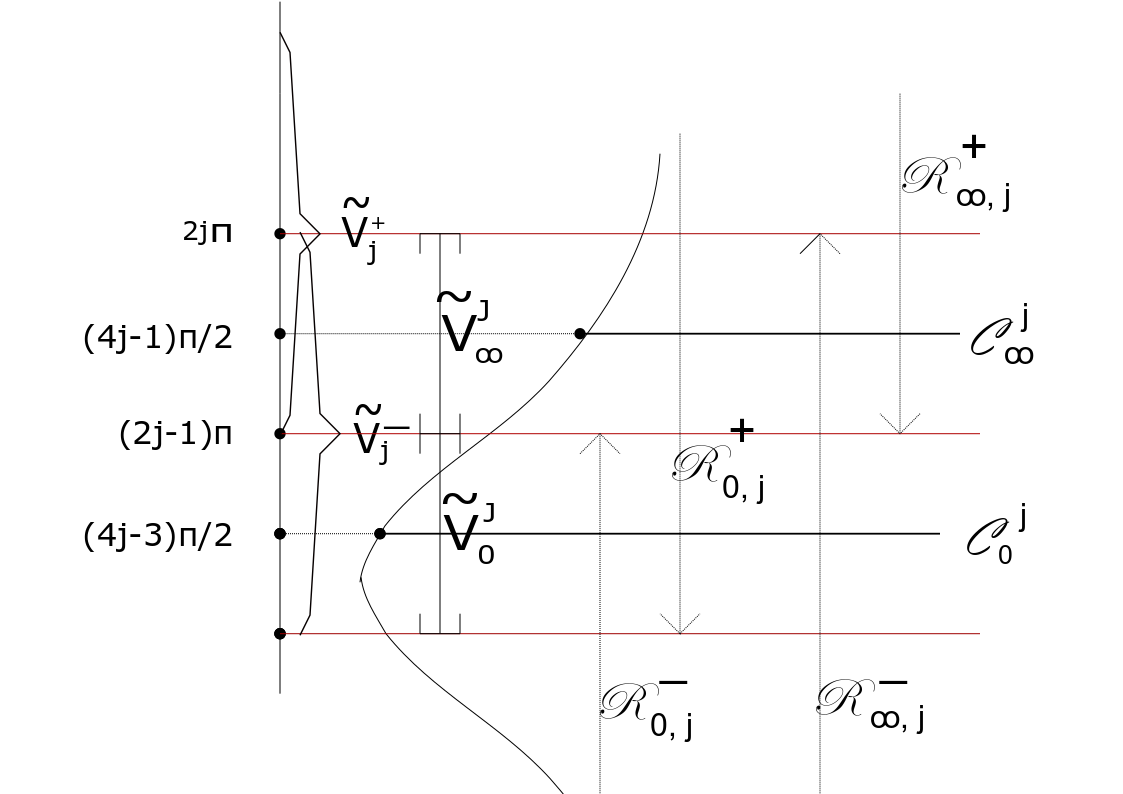
Figure 3.1. The outline of position of petals $\tilde{V}_{j}^{\pm}$ and $\tilde{V}_{0,\infty}^{j}$, $j\in\mathbb{Z}$, on a standard quadratic domain $\widetilde{\mathcal{R}}_{C}$ in the logarithmic chart.

Proof.

We use Cauchy-Heine’s construction based on the classical Cauchy’s residue theorem. For more details on Cauchy-Heine construction in $\mathbb{C}$ that we adapt here for standard quadratic (linear) domains, see e.g. [4] or [5].

$(1)$ Obvious.

$(2)$ Suppose that we wish to extend $\tilde{F}_{0,j}^{-}$ above the central line $\mathcal{C}_{0}^{j}$ of petal $\tilde{V}_{0}^{j}$. We replace the integration path $\mathcal{C}_{0}^{j}$ in the Cauchy-Heine integral by the union of a horizontal line $\big{(}\mathcal{C}_{0}^{j}\big{)}^{\prime}$ above $\mathcal{C}_{0}^{j}$ in $\tilde{V}_{0}^{j}$ and the portion of the boundary of the petal $\tilde{V}_{0}^{j}$ between the two lines, denoted by $\mathcal{S}_{0}^{j}$, see Figure 3.1 and Figure 3.2. Here, $\big{(}\mathcal{C}_{0}^{j}\big{)}^{\prime}$ is a horizontal line at some height $\theta\in\big{(}(4j-3)\frac{\pi}{2},(2j-1)\pi\big{)}$ in the standard quadratic domain in the $\zeta$-variable. It corresponds, in the $z$-variable, to the ray at angle $\theta$ inside the petal $V_{0}^{j}$. For simplicity, we are notationally imprecise, as we do not stress the dependence of $\big{(}\mathcal{C}_{0}^{j}\big{)}^{\prime}$ and $\mathcal{S}_{0}^{j}$ on the height $\theta$. Let $\gamma_{\theta}:=(\mathcal{C}_{0}^{j})^{\prime}\cup\mathcal{S}_{0}^{j}$ be this new integration path. Then, for any $\zeta$ below $\mathcal{C}_{0}^{j}$, the Cauchy-Heine integral along $\gamma_{\theta}$ is, by the Cauchy’s integral theorem, equal to $\tilde{F}_{0,j}^{-}$. That is, for $\zeta\in\widetilde{\mathcal{R}}_{C}$ below $\mathcal{C}_{0}^{j}$, we get:

$$\tilde{F}_{0,j}^{-}(\zeta):=\frac{1}{2\pi i}\int_{\mathcal{C}_{0}^{j}}\frac{\tilde{G}_{0}^{j}(w)}{w-\zeta}dw =\frac{1}{2\pi i}\int_{\gamma_{\theta}}\frac{\tilde{G}_{0}^{j}(w)}{w-\zeta}d\zeta$$

$$=\frac{1}{2\pi i}\int_{(\mathcal{C}_{0}^{j})^{\prime}}\frac{\tilde{G}_{0}^{j}(w)}{w-\zeta}dw+\frac{1}{2\pi i}\int_{\mathcal{S}_{0}^{j}}\frac{\tilde{G}_{0}^{j}(w)}{w-\zeta}dw,$$

see Figure 3.2.

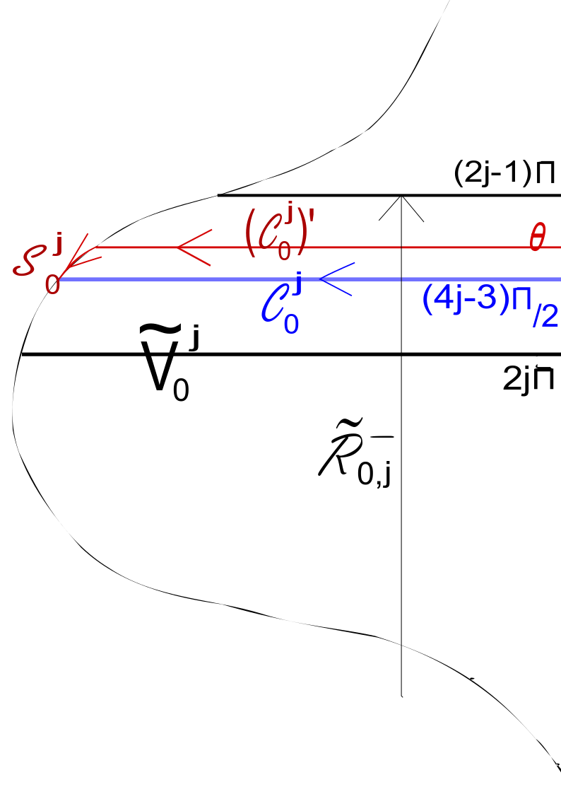
Figure 3.2. The change of integration path in the $\zeta$-variable and Cauchy’s integral theorem in the proof of Lemma 3.3 $(2)$.

Therefore, the new integral $\int_{\gamma_{\theta}}\frac{\tilde{G}_{0}^{j}(w)}{w-\zeta}dw$ along $\gamma_{\theta}$ is the analytic extension of $\tilde{F}_{0,j}^{-}$ up to the line $(\mathcal{C}_{0}^{j})^{\prime}$. By varying the line $(\mathcal{C}_{0}^{j})^{\prime}$ above the central line $\mathcal{C}_{0}^{j}$ inside the petal $\tilde{V}_{0}^{j}$, we get the desired analytic extension up to the line at height $(2j-1)\pi$. In this way, $\tilde{F}_{0,j}^{-}(\zeta)$ given by formula (LABEL:eq:ch) can be extended analytically to whole $\widetilde{\mathcal{R}}_{0,j}^{-}$. The same can be done for $\tilde{F}_{0,j}^{+}(\zeta)$ on $\widetilde{\mathcal{R}}_{0,j}^{+}$ and for $\tilde{F}_{\infty,j}^{\pm}(\zeta)$ on $\widetilde{\mathcal{R}}_{\infty,j}^{\pm}$, $j\in\mathbb{Z}$.

If we now denote by

$$\tilde{\chi}_{0}^{j}(\zeta):=\frac{1}{2\pi i}\int_{\mathcal{S}_{0}^{j}}\frac{\tilde{G}_{0}^{j}(w)}{w-\zeta}dw,$$

we notice that $\tilde{\chi}_{0}^{j}(\zeta)$ is an analytic germ at $\zeta=\infty$ (in the sense that $\xi\mapsto\tilde{\chi}_{0}^{j}(\frac{1}{\xi})$ is analytic at $\xi=0$), that is, that there exists $M_{j}>0$ such that $\tilde{\chi}_{0}^{j}(\zeta)$ is analytic for $\zeta\in\mathbb{C},\ |\zeta|>M_{j}$. Consequently, it admits a Taylor asymptotic expansion in $\zeta^{-1}$, as $|\zeta|\to\infty$. This will be important for later proofs.

We stress once again that here $(\mathcal{C}_{0}^{j})^{\prime}$ and $\mathcal{S}_{0}^{j}$, and therefore also $\tilde{\chi}_{0}^{j}(\zeta)$ and $M_{j}$, depend on the height $\theta$ of the line $(\mathcal{C}_{0}^{j})^{\prime}$ up to which we extend. They are not dependent only on the petal, but also on the height in the petal up to which we extend. Here and in the sequel, we omit this dependence in the notation for simplicity.

(3) Since $\tilde{V}_{0}^{j}=\widetilde{\mathcal{R}}_{0,j}^{+}\cap\widetilde{\mathcal{R}}_{0,j}^{-},\ \tilde{V}_{\infty}^{j}=\widetilde{\mathcal{R}}_{\infty,j}^{+}\cap\widetilde{\mathcal{R}}_{\infty,j}^{-}$, (LABEL:eq:ahhh) follows directly by the residue theorem after analytic extensions of $\tilde{F}_{0,\infty}^{\pm}(\zeta)$ to $\widetilde{\mathcal{R}}_{0,\infty,j}^{\pm}$ described in $(2)$. To illustrate, let us prove the first line of (LABEL:eq:ahhh). Take any $\zeta\in\tilde{V}_{0}^{j}$. Take any two lines inside petal $\tilde{V}_{0}^{j}$ such that $\zeta$ is strictly between them. Denote them by $\mathcal{C}_{\theta_{1}}$ and $\mathcal{C}_{\theta_{2}}$, at heights $\theta_{1}>\theta_{2}$. Now, by part $(2)$, we have:

$$\tilde{F}_{0,j}^{+}(\zeta) =\frac{1}{2\pi i}\int_{\mathcal{C}_{\theta_{2}}}\frac{\tilde{G}_{0}^{j}(w)}{w-\zeta}dw+\frac{1}{2\pi i}\int_{\mathcal{S}_{\theta_{2}}}\frac{\tilde{G}_{0}^{j}(w)}{w-\zeta}dw,$$

$$\tilde{F}_{0,j}^{-}(\zeta) =\frac{1}{2\pi i}\int_{\mathcal{C}_{\theta_{1}}}\frac{\tilde{G}_{0}^{j}(w)}{w-\zeta}dw+\frac{1}{2\pi i}\int_{\mathcal{S}_{\theta_{1}}}\frac{\tilde{G}_{0}^{j}(w)}{w-\zeta}dw,$$

where $\mathcal{S}_{\theta_{1}}$ resp. $\mathcal{S}_{\theta_{2}}$ are the portions of the boundary of $\tilde{V}_{0}^{j}$ between the lines $\mathcal{C}_{0}^{j}$ and $\mathcal{C}_{\theta_{1}}$ and between $\mathcal{C}_{0}^{j}$ and $\mathcal{C}_{\theta_{2}}$ respectively. Subtracting $\tilde{F}_{0,j}^{+}(\zeta)-\tilde{F}_{0,j}^{-}(\zeta)$, the statement follows by the residue theorem. See Figure 3.3.

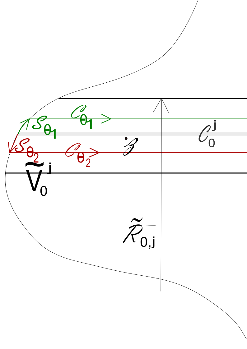
Figure 3.3. The residue theorem in the proof of Lemma 3.3 $(3)$.

∎

Lemma 3.4.

Let $(\tilde{G}_{0}^{j},\tilde{G}_{\infty}^{j})_{j\in\mathbb{Z}}$ be an infinite cocycle as described in Propositions 3.1 or 3.2. Let $\tilde{F}_{0,j}^{\pm},\ \tilde{F}_{\infty,j}^{\pm}$ and their corresponding domains $\widetilde{\mathcal{R}}_{0,j}^{\pm},\ \widetilde{\mathcal{R}}_{\infty,j}^{\pm}$ be as defined in Lemma 3.3. Let

(3.14) $$\tilde{R}_{j}^{+}:=\Big{(}\big{(}\sum_{k=-\infty}^{j}\tilde{F}_{0,k}^{+}+\sum_{k=-\infty}^{j}\tilde{F}_{\infty,k}^{+}\big{)}+\big{(}\sum_{k=j+1}^{+\infty}\tilde{F}_{0,k}^{-}+\sum_{k=j+1}^{+\infty}\tilde{F}_{\infty,k}^{-}\big{)}\Big{)}\Big{|}_{\tilde{V}_{j}^{+}}\Big{.},\ j\in\mathbb{Z},$$

$$\tilde{R}_{j}^{-}:=\Big{(}\big{(}\sum_{k=-\infty}^{j}\tilde{F}_{0,k}^{+}+\sum_{k=-\infty}^{j-1}\tilde{F}_{\infty,k}^{+}\big{)}+\big{(}\sum_{k=j+1}^{+\infty}\tilde{F}_{0,k}^{-}+\sum_{k=j}^{+\infty}\tilde{F}_{\infty,k}^{-}\big{)}\Big{)}\Big{|}_{\tilde{V}_{j}^{-}}\Big{.},\ j\in\mathbb{Z}.$$

Then $\tilde{R}_{j}^{\pm}$ are well-defined analytic functions on petals $\tilde{V}_{j}^{\pm}$, $j\in\mathbb{Z}$.

Moreover, the functions $\tilde{R}_{j}^{\pm}$ realize the cocycle $(\tilde{G}_{0}^{j},\tilde{G}_{\infty}^{j})_{j\in\mathbb{Z}}$:

(3.15) $$\begin{split}&\tilde{R}_{j-1}^{+}(\zeta)-\tilde{R}_{j}^{-}(\zeta)=\tilde{G}_{0}^{j}(\zeta),\ \zeta\in\tilde{V}_{0}^{j},\\ &\tilde{R}_{j}^{-}(\zeta)-\tilde{R}_{j}^{+}(\zeta)=\tilde{G}_{\infty}^{j}(\zeta),\ \zeta\in\tilde{V}_{\infty}^{j},\ \ j\in\mathbb{Z}.\end{split}$$

As shown in Figure 3.4 below, to get functions $\tilde{R}_{j}^{\pm}$ defined by (3.14) on $\tilde{V}_{j}^{\pm}$, on corresponding petal (strip) $\tilde{V}_{j}^{\pm}$ we sum all functions $\tilde{F}_{0,k}^{\pm}$, $\tilde{F}_{\infty,k}^{\pm}$, $k\in\mathbb{Z}$, from (LABEL:eq:ch) which are well-defined on $\tilde{V}_{j}^{\pm}$.

The proof of Lemma 3.4 is in the Appendix. We prove that, for every $j\in\mathbb{Z}$, the series in (3.14) converges uniformly on compacts in $\tilde{V}_{j}^{\pm}$, thus defining analytic functions $\tilde{R}_{j}^{\pm}$ on $\tilde{V}_{j}^{\pm}$ by the Weierstrass theorem.

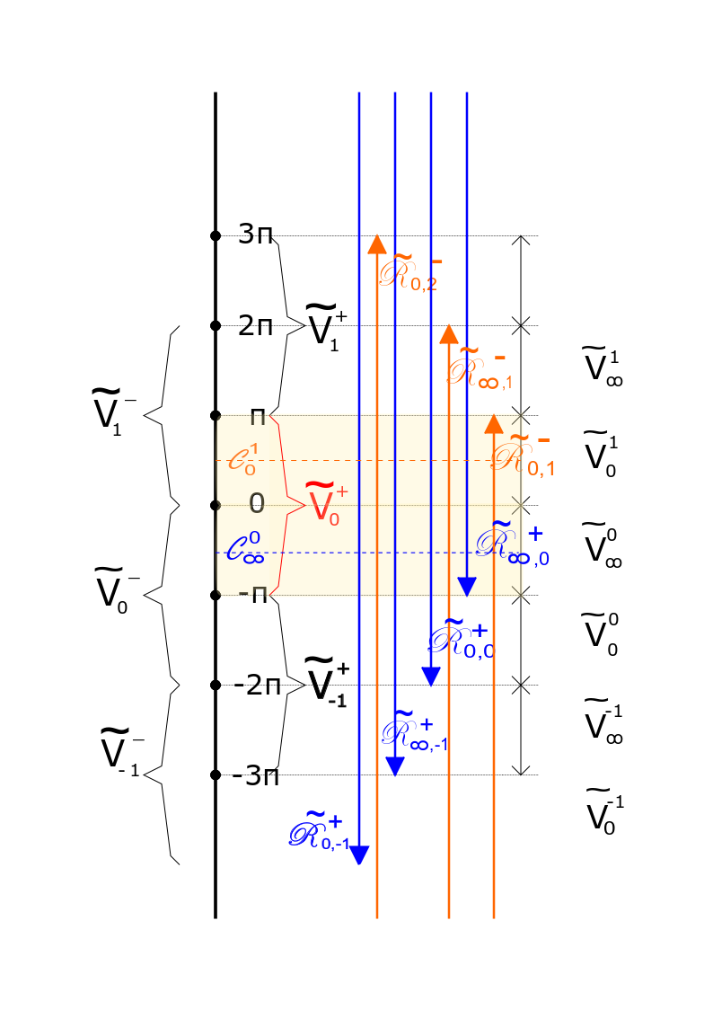
Figure 3.4. Ilustration of formula (3.14) for $\tilde{R}_{0}^{+}$ on $\tilde{V}_{0}^{+}$. The figure illustrates in which domains $\widetilde{\mathcal{R}}_{0/\infty,j}^{\pm}$ the petal $\tilde{V}_{0}^{+}$ is fully contained. To get $\tilde{R}_{0}^{+}$, we sum the corresponding functions $\tilde{F}_{0/\infty,j}^{\pm}$ from (LABEL:eq:ch).

We prove in Lemma 3.5 below the asymptotics for $\tilde{R}_{j}^{\pm}$ constructed on $\tilde{V}_{j}^{\pm}$ in Lemma 3.4. It holds that $\tilde{R}_{j}^{\pm}(\zeta)=o(1)$, as $\text{Re}(\zeta)\to\infty$ in $\tilde{V}_{j}^{\pm}$, moreover uniformly in $j\in\mathbb{Z}$. Also, for standard linear domains we show additionaly the complete $\log$-Gevrey asymptotic expansion of $\tilde{R}_{j}^{\pm}(\zeta)$ in $\mathbb{C}[[\zeta^{-1}]]$, as $\text{Re}(\zeta)\to\infty$ on $\tilde{V}_{j}^{\pm}$.

Lemma 3.5 ($\log$-Gevrey asymptotic expansion of $\tilde{R}_{j}^{\pm}(\zeta),\ j\in\mathbb{Z}$).

Let $\tilde{R}_{j}^{\pm},\ j\in\mathbb{Z}$, be constructed as in Lemma 3.4 on petals $\tilde{V}_{j}^{\pm}$ on a standard quadratic or a standard linear domain. Then:

1. On both domains $($standard linear and standard quadratic$)$, there exist subdomains $($linear resp. quadratic$)$ $\widetilde{\mathcal{R}}_{C^{\prime}}\subset\widetilde{\mathcal{R}}_{C}$ such that, for substrips $\tilde{U}_{j}\subset\tilde{V}_{j}^{\pm}\cap\widetilde{\mathcal{R}}_{C^{\prime}}$ centered at center lines of $\tilde{V}_{j}^{\pm}$ and of width $0<\theta<2\pi$ independent of $j\in\mathbb{Z}$, there exists a uniform in $j\in\mathbb{Z}$ constant $C_{\theta}>0$ such that:

   $$|\tilde{R}_{j}^{\pm}(\zeta)|\leq C_{\theta}|\zeta|^{-1},\ \zeta\in\tilde{U}_{j}.$$

2. If $\tilde{R}_{j}^{\pm}$ are constructed on a standard linear domain, then there exists a formal series $\widehat{R}\in\mathbb{C}[[\zeta^{-1}]]$, such that any $\tilde{R}_{j}^{\pm}(\zeta),\ j\in\mathbb{Z},$ admits $\widehat{R}$ as its $\log$-Gevrey asymptotic expansion of order $m$, as $\text{Re}(\zeta)\to+\infty$ in $\tilde{V}_{j}^{\pm}$. Here, $m>0$ is given in (3.4).

The proof is in the Appendix. Also, in Remark 7.3 in the Appendix we show a technical obstacle for proving statement $(2)$ on a standard quadratic domain.

Proof of Propositions 3.1 and 3.2. Let $\tilde{R}_{j}^{\pm}$ be as constructed in Lemma 3.4 on petals $\tilde{V}_{j}^{\pm}$ in the $\zeta$-variable, $j\in\mathbb{Z}$, either on a standard quadratic or a standard linear domain. Returning to the variable $z=e^{-\zeta}$, we put:

$$R_{j}^{\pm}(z):=\tilde{R}_{j}^{\pm}(\zeta),\ z\in V_{j}^{\pm},\ j\in\mathbb{Z}.$$

By Lemma 3.4, $R_{j}^{\pm}(z)$ are analytic on $V_{j}^{\pm}$ and we have:

(3.16) $$\begin{split}&R_{+}^{j-1}(z)-R_{-}^{j}(z)=G_{0}^{j}(z),\ z\in V_{0}^{j},\\ &R_{-}^{j}(z)-R_{+}^{j}(z)=G_{\infty}^{j}(z),\ z\in V_{\infty}^{j},\ \ j\in\mathbb{Z}.\end{split}$$

Moreover, putting $\boldsymbol{\ell}:=\zeta^{-1}$, from Lemma 3.5 we get that the functions $\breve{R}_{j}^{\pm}(\boldsymbol{\ell}):=R_{j}^{\pm}(z)$ constructed on a standard linear domain on $\boldsymbol{\ell}$-cusps $\boldsymbol{\ell}(V_{j}^{\pm})$, $j\in\mathbb{Z}$, admit a $\log$-Gevrey power asymptotic expansion of order $m$. By exponentially small differences (LABEL:eq:es) on intersections of petals, we get that all $\breve{R}_{j}^{\pm}(\boldsymbol{\ell})$ admit a common $\widehat{R}(\boldsymbol{\ell})\in\mathbb{C}[[\boldsymbol{\ell}]]$ as their $\log$-Gevrey asymptotic expansion of order $m$. The uniform bound (3.6) for both domains (linear and quadratic) follows by statement $(1)$ of Lemma 3.5. Thus Propositions 3.1 and 3.2 are proven. $\Box$

Remark 3.6.

Observe that the functions $R_{j}^{\pm}(z)$ constructed in the proof of Proposition 3.2 by Cauchy-Heine integrals on petals along standard linear domain are not petalwise restrictions of $R_{j}^{\pm}(z)$ constructed along standard quadratic domain in the proof of Proposition 3.1.

Indeed, the lines of integration $\mathcal{C}_{0,\infty}^{k}$ are changed (asymptotically shorter for standard linear domains). Therefore, we cannot claim that $R_{j}^{\pm}$ defined on petals of a standard linear domain can be analytically extended to petals of a standard quadratic domain. Therefore, we do not claim in Proposition 3.1 that there exist $\breve{R}_{j}^{\pm}(\boldsymbol{\ell})$ defined on $\boldsymbol{\ell}$-images of petals of a larger standard quadratic domain which admit a $\log$-Gevrey asymptotic expansion, as $\boldsymbol{\ell}\to 0$.

4. Proof of Theorem A

The proof is very involved, so we first give an outline of the proof. We then state necessary lemmas, and prove Theorem A at the end of the section.

Outline of the proof of Theorem A. Let $(h_{0}^{j},h_{\infty}^{j};\sigma_{j})_{j\in\mathbb{Z}}$ be a symmetric sequence (1.10) of analytic germs of diffeomorphisms from $\mathrm{Diff}(\mathbb{C},0)$, satisfying the uniform bound (2.4). Let $\rho\in\mathbb{R}$ and $m\in\mathbb{Z}$. Here we construct a parabolic germ $f$, defined on a standard quadratic domain, of the prenormalized form

$$f(z)=z-z^{2}\boldsymbol{\ell}^{m}+\rho z^{3}\boldsymbol{\ell}^{2m+1}+o(z^{3}\boldsymbol{\ell}^{2m+1}),\ z\in\mathcal{R}_{C},$$

whose sectorial Fatou coordinates realize the given sequence as its horn maps. Let $V_{j}^{+}$ resp. $V_{j}^{-}$, $j\in\mathbb{Z}$, be petals covering a standard quadratic domain of opening $2\pi$, centered at $2j\pi$ resp. $(2j-1)\pi$, and let $V_{0}^{j}:=V_{j-1}^{+}\cap V_{j}^{-}$, $V_{\infty}^{j}:=V_{j}^{+}\cap V_{j}^{-}$ be their intersecting petals of opening $\pi$, as shown in Figure 1.4. We construct $f$ by constructing its sectorial Fatou coordinates $\Psi_{\pm}^{j}$ on $V_{j}^{\pm},\ j\in\mathbb{Z}$, in an iterative construction described below, which satisfy:

(4.1) $$\begin{split}&\Psi_{j-1}^{+}(z)-\Psi_{j}^{-}(z)=g_{0}^{j}(e^{-2\pi i\Psi_{j-1}^{+}(z)}),\ z\in V_{0}^{j},\\ &\Psi_{j}^{-}(z)-\Psi_{j}^{+}(z)=g_{\infty}^{j}(e^{2\pi i\Psi_{j}^{+}(z)}),\ z\in V_{\infty}^{j},\ \ j\in\mathbb{Z}.\end{split}$$

Here, $g_{0}^{j},\ g_{\infty}^{j},\ j\in\mathbb{Z}$, are analytic germs at $t\approx 0$, related to given $h_{0}^{j},\ h_{\infty}^{j}$, $j\in\mathbb{Z}$, by:

(4.2) $$(h_{0}^{j})^{-1}(t)=te^{2\pi ig_{0}^{j}(t)},\ h_{\infty}^{j}(t)=te^{2\pi ig_{\infty}^{j}(t)},\ t\approx 0.$$

Then, due to (LABEL:eq:fatouu) and (4.2), $f$ realizes the sequence of pairs of diffeomorphisms $(h_{0}^{j},h_{\infty}^{j})_{j\in\mathbb{Z}}$ as its horn maps. Indeed, (LABEL:eq:fatouu) is an equivalent formulation of this statement, see Subsection 2.1 for more details.

The idea of successive approximations is taken from [11] for realizing the moduli of analytic classification for saddle-node vector fields. We will use the cocycle realization Proposition 3.1 and, by Lemma 4.1 (1), iteratively realize the cocycles $({}^{n}G_{0}^{j},{}^{n}G_{\infty}^{j})_{j\in\mathbb{Z}}$, $n\in\mathbb{N}_{0}$, where

$${}^{n}G_{0}^{j}(z): =g_{0}^{j}(e^{-2\pi i\Psi_{j-1,+}^{n}(z)}),\ z\in V_{0}^{j},$$

$${}^{n}G_{\infty}^{j}(z): =g_{\infty}^{j}(e^{2\pi i\Psi_{j,+}^{n}(z)}),\ z\in V_{\infty}^{j}.$$

Here, $(\Psi_{j,\pm}^{n})_{n\in\mathbb{N}_{0}}$ on $V_{\pm}^{j}$ are successive approximations of the final Fatou coordinate $\Psi_{j}^{\pm}$, $j\in\mathbb{Z}$, starting with the Fatou coordinate of the $(2,m,\rho)$-formal normal form $\Psi_{j,\pm}^{0}:=\Psi_{\mathrm{nf}}$ on $V_{\pm}^{j}$. More precisely, we construct them as follows:

$$\Psi_{j,\pm}^{n}(z):=\Psi_{\mathrm{nf}}(z)+R_{j,\pm}^{n}(z),\ z\in V_{\pm}^{j},\ n\in\mathbb{N},$$

where

(4.3) $$\begin{split}&R_{j,\pm}^{0}(z):=0,\ z\in V_{\pm}^{j},\text{ and}\\ &R_{j-1,+}^{n}(z)-R_{j,-}^{n}(z)=g_{0}^{j}(e^{-2\pi i\Psi_{j-1,+}^{n-1}(z)}):={}^{n-1}G_{0}^{j}(z),\ z\in V_{0}^{j},\\ &R_{j,-}^{n}(z)-R_{j,+}^{n}(z)=g_{\infty}^{j}(e^{2\pi i\Psi_{j,+}^{n-1}(z)}):={}^{n-1}G_{\infty}^{j}(z),\ z\in V_{\infty}^{j},\ n\in\mathbb{N}.\end{split}$$

At each step $n$, the functions $R_{j,\pm}^{n}(z)=o(1)$, $z\to 0$, are obtained using Proposition 3.1 for the realization of the previous cocycle $({}^{n-1}G_{0}^{j},{}^{n-1}G_{\infty}^{j})_{j\in\mathbb{Z}}$. The cocycle itself is obtained by applying $g_{0}^{j},\ g_{\infty}^{j}$ to the exponentials of the Fatou coordinates from the previous step. In this manner, we make corrections of the Fatou coordinate at each step, starting from the natural initial choice $\Psi_{\mathrm{nf}}$, the Fatou coordinate of the fomal normal form.

We then prove, in Lemma 4.1 (2), the uniform convergence of the Fatou coordinates $\Psi_{j,\pm}^{n}$ (that is, of $R_{j,\pm}^{n}$), as $n\to\infty$, on compact subsectors of petals $V_{\pm}^{j}$. Thus, as limits, we get analytic Fatou coordinates, which we denote by $\Psi_{j}^{\pm}:=\Psi_{\mathrm{nf}}+R_{j}^{\pm}$, on petals $V_{j}^{\pm}$. By taking pointwise limit, as $n\to\infty$, to (LABEL:eq:lim), we get that $\Psi_{j}^{\pm}$ satisfy (LABEL:eq:fatouu) and thus realize the given sequence of pairs of horn maps $(h_{0}^{j},h_{\infty}^{j})_{j\in\mathbb{Z}}$.

Finally, we recover the germ $f$ from its sectorial Fatou coordinates, using the Abel equation. On each petal, $f(z):=(\Psi_{j}^{\pm})^{-1}\big{(}1+\Psi_{j}^{\pm}\big{(}z)\big{)},\ z\in V_{j}^{\pm}$. We show that $f$ glues to an analytic function on a standard quadratic domain. It is of the prenormalized form (2.7) due to the form of $\Psi_{j}^{\pm}:=\Psi_{\mathrm{nf}}+R_{j}^{\pm},\ R_{j}^{\pm}=o(1)$, as $z\to 0$ on $V_{j}^{\pm}$, and Proposition 7.1 in the Appendix. The uniform bound (2.3) is proven by Lemma 4.1 (3). To prove Lemma 4.1 (3), we prove that the uniform bound (3.6) from Proposition 3.1 holds with the same constant for $R_{j,\pm}^{n}$ in each iterative step $n\in\mathbb{N}$.

We prove in Lemma 4.5 that symmetry of horn maps (1.10) implies that $\mathbb{R}_{+}$ is invariant by $f$.

4.1. The main lemmas

Lemma 4.1.

Let $(h_{0}^{j},h_{\infty}^{j};\sigma_{j})_{j\in\mathbb{Z}}$, where

$$\sigma_{j}\geq K_{1}e^{-Ke^{C\sqrt{|j|}}},\ |j|\to\infty,\text{ for some $C,\ K,\ K_{1}>0$},$$

be a symmetric sequence (1.10) of pairs of analytic germs from $\mathrm{Diff}(\mathbb{C},0)$, satisfying the uniform bound (2.4). Let the sequence of pairs of analytic germs of diffeomorphisms $(g_{0}^{j},g_{\infty}^{j};\sigma_{j})_{j\in\mathbb{Z}}$ be defined from $(h_{0}^{j},h_{\infty}^{j};\sigma_{j})_{j\in\mathbb{Z}}$ by (4.2). Let $\rho\in\mathbb{R}$ and $m\in\mathbb{Z}$, and let $\Psi_{\mathrm{nf}}$ be the Fatou coordinate of the $(2,\rho,m)$-model $f_{0}$ from (2.1). Let $\{V_{j}^{\pm}\}_{j\in\mathbb{Z}}$ be a collection of petals of opening $2\pi$, centered at $j\pi$, along a standard quadratic domain.

1. The following sequence of analytic maps $\Psi_{j,\pm}^{n}$, $n\in\mathbb{N}_{0}$, on petals $V_{j}^{\pm}$, is well-defined by the following iterative procedure:

   $$\Psi_{j,\pm}^{n}(z):=\Psi_{\mathrm{nf}}(z)+R_{j,\pm}^{n}(z),\ z\in V_{\pm}^{j},\ n\in\mathbb{N}_{0},$$

   where

   (4.4) $$\begin{split}&R_{j,\pm}^{0}(z):=0,\ z\in V_{j}^{\pm},\text{ and}\\ &R_{j-1,+}^{n}(z)-R_{j,-}^{n}(z)=g_{0}^{j}(e^{-2\pi i\Psi_{j-1,+}^{n-1}(z)})=:{}^{n-1}G_{0}^{j}(z),\ z\in V_{0}^{j},\\ &R_{j,-}^{n}(z)-R_{j,+}^{n}(z)=g_{\infty}^{j}(e^{2\pi i\Psi_{j,+}^{n-1}(z)})=:{}^{n-1}G_{\infty}^{j}(z),\ z\in V_{\infty}^{j},\ n\in\mathbb{N}.\end{split}$$

   Here, for every $n\in\mathbb{N}$, $\big{(}^{n-1}G_{0}^{j}(z),^{n-1}G_{\infty}^{j}(z)\big{)}_{j\in\mathbb{Z}}$ is an infinite cocycle satisfying all assumptions of Proposition 3.1, and $R_{j,\pm}^{n},\ n\in\mathbb{N},$ are analytic germs on petals $V_{j}^{\pm}$, $j\in\mathbb{Z}$, that realize this cocycle, given by Proposition 3.1.

2. For every $j\in\mathbb{Z}$, the sequence $(\Psi_{j,\pm}^{n})_{n\in\mathbb{N}}$ converges uniformly on compact subsectors of $V_{j}^{\pm}$, thus defining analytic functions $\Psi_{j}^{\pm}$ on petals $V_{j}^{\pm}$ at the limit. Moreover, $\Psi_{j}^{\pm}$, $j\in\mathbb{Z}$, satisfy:

   (4.5) $$\begin{split}&\Psi_{j-1}^{+}(z)-\Psi_{j}^{-}(z)=g_{0}^{j}(e^{-2\pi i\Psi_{j-1}^{+}(z)}),\ z\in V_{0}^{j},\\ &\Psi_{j}^{-}(z)-\Psi_{j}^{+}(z)=g_{\infty}^{j}(e^{2\pi i\Psi_{j}^{+}(z)}),\ z\in V_{\infty}^{j},\ \ j\in\mathbb{Z}.\end{split}$$

3. For the petalwise limits $R_{j}^{\pm}$, $j\in\mathbb{Z}$, the following uniform bound holds. For every collection of subsectors $S_{j}\subset V_{j}^{\pm}$ centered at $j\pi$ and of opening strictly less than $2\pi$ independent of $j\in\mathbb{Z}$, there exists a uniform constant $C>0$ $($independent of $j)$, such that:

   (4.6) $$|R_{j}^{\pm}(z)|\leq C|\boldsymbol{\ell}|,\ z\in S_{j},\ j\in\mathbb{Z}.$$

For simplicity, in the proof of Lemma 4.1, we pass to the logarithmic chart. We denote by $\tilde{V}_{j}^{\pm}$ the petals $V_{j}^{\pm}$ in the logarithmic chart. Let

(4.7) $$\tilde{\Psi}_{j,\pm}^{n}(\zeta):=\Psi_{j,\pm}^{n}(e^{-\zeta}),\ \tilde{R}_{j,\pm}^{n}(\zeta):=R_{j,\pm}^{n}(e^{-\zeta}),\ \zeta\in\tilde{V}_{j}^{\pm},\ j\in\mathbb{Z},\ n\in\mathbb{N}.$$

In the proof of statement $(2)$ in Lemma 4.1, we use the following auxiliary lemma, whose proof is in the Subsection 7.4 of the Appendix. Due to a technical detail in the Cauchy-Heine construction (the presence of a logarithmic singularity at the border of the standard quadratic domain), we are unable to prove uniform convergence of $(\tilde{R}_{j,\pm}^{n})_{n}$ on $\tilde{V}_{j}^{\pm}$, as $n\to\infty$. Instead, we prove uniform convergence of their exponentials on petals, which then implies uniform convergence on compact subsets for the initial sequence.

Lemma 4.2.

Let the assumptions of Lemma 4.1 hold. Let $\tilde{R}_{j,\pm}^{n}$, $n\in\mathbb{N}$, be as defined in the statement $(1)$ of Lemma 4.1 $($in the logarithmic chart, see (4.7)$)$. The sequence

$$\big{(}e^{2\pi i\tilde{R}_{j,\pm}^{n}}\big{)}_{n\in\mathbb{N}}$$

is a Cauchy sequence in the sup-norm on petal $\tilde{V}_{j}^{\pm}$, for every $j\in\mathbb{Z}$.

Proof of Lemma 4.1.

Proof of statement $(1)$. We check that, in every step of the construction, all assumptions of Proposition 3.1 are satisfied. The basis of the induction is obvious by putting $\tilde{R}_{j,\pm}^{0}\equiv 0,\ \tilde{\Psi}_{j,\pm}^{0}:=\tilde{\Psi}_{\mathrm{nf}}$ on $\tilde{V}_{\pm}^{j}$. Suppose that $\tilde{\Psi}_{j,\pm}^{k}$ are constructed and analytic for $0\leq k<n$. By Remark 7.5 in the Appendix and the uniform bound (2.5) on $g_{0}^{j}$, we get that there exist constants $c>0$ and $C_{1}>0$ independent of $j\in\mathbb{Z}$, such that:

(4.8) $$\big{|}{}^{n-1}\tilde{G}_{0}^{j}(\zeta)\big{|}=\Big{|}g_{0}^{j}\big{(}e^{-2\pi i\tilde{\Psi}_{j-1,+}^{n-1}(e^{-\zeta})}\big{)}\Big{|}\leq c\big{|}e^{-2\pi i\Psi_{j-1,+}^{n-1}(e^{-\zeta})}\big{|} \leq C_{1}\big{|}e^{-\pi i\tilde{\Psi}_{\mathrm{nf}}(\zeta)}\big{|}$$

$$=C_{1}e^{\pi\text{Im}(\tilde{\Psi}_{\mathrm{nf}}(\zeta))},\ \zeta\in\tilde{V}_{0}^{j}.$$

Now, for every collection of central substrips $\tilde{U}_{j}\subset\tilde{V}_{0}^{j}$ of width independent of $j\in\mathbb{Z}$ and for every $\delta>0$, there exist constants $C,\,D>0$ independent of $j\in\mathbb{Z}$ such that:

(4.9) $$\big{|}\mathrm{Im}(\tilde{\Psi}_{\mathrm{nf}}(\zeta))\big{|}=-\mathrm{Im}(\tilde{\Psi}_{\mathrm{nf}}(\zeta))\geq C|\tilde{\Psi}_{\mathrm{nf}}(\zeta)|\geq De^{(1-\delta)\mathrm{Re}(\zeta)},\ \zeta\in\tilde{U}_{j}.$$

The last inequality is obtained using the exact form of $\Psi_{\mathrm{nf}}(z)$ given in (7.1) and the fact that, for a standard quadratic domain $\widetilde{\mathcal{R}}_{C}$, there exists $d>0$ such that $\mathrm{Im}(\zeta)\leq d\cdot\mathrm{Re}^{2}(\zeta)$, $\zeta\in\widetilde{\mathcal{R}}_{C}$.

Therefore, combining (4.8) and (4.9), for a collection of substrips $\tilde{U}_{j}\subset\tilde{V}_{0}^{j}$ of a given width $0<\theta<2\pi$ independent of $j\in\mathbb{Z}$, there exist constants $C,\ M>0$ independent of $j\in\mathbb{Z}$ and of the step $n\in\mathbb{N}$, such that:

(4.10) $$\big{|}{}^{n-1}\tilde{G}_{0}^{j}(\zeta)\big{|}\leq Ce^{-Me^{(1-\delta)\mathrm{Re}(\zeta)}},\ \zeta\in\tilde{U}_{j},\ j\in\mathbb{Z},\ n\in\mathbb{N}.$$

A similar analysis is done for ${}^{n-1}\tilde{G}_{\infty}^{j}(\zeta)$ on $\tilde{V}_{\infty}^{j}$, $j\in\mathbb{Z}$. Therefore, assumption (3.4) of Proposition 3.1 is satisfied in every step with $m=1-\delta$, for every $\delta>0$. The existence and analyticity of $\tilde{R}_{j,\pm}^{n}$ on $\tilde{V}_{j}^{\pm}$ then follows directly by Proposition 3.1. Also, (LABEL:e:pp) follows directly from (LABEL:e:p) in Proposition 3.1.

Precisely, for later use, by Lemma 3.4 in the proof of Proposition 3.1, $\tilde{R}_{j,\pm}^{n}$ on petals $\tilde{V}_{j}^{\pm}$, $j\in\mathbb{Z}$, $n\in\mathbb{N}$, are given as the sum of the Cauchy-Heine integrals as follows:

(4.11) $$\tilde{R}_{j,+}^{n}:=\Big{(}\big{(}\sum_{k=-\infty}^{j}{}^{n}\tilde{F}_{0,k}^{+}+\sum_{k=-\infty}^{j}{}^{n}\tilde{F}_{\infty,k}^{+}\big{)}+\big{(}\sum_{k=j+1}^{+\infty}{}^{n}\tilde{F}_{0,k}^{-}+\sum_{k=j+1}^{+\infty}{}^{n}\tilde{F}_{\infty,k}^{-}\big{)}\Big{)}\Big{|}_{\tilde{V}_{j}^{+}}\Big{.},$$

$$\tilde{R}_{j,-}^{n}:=\Big{(}\big{(}\sum_{k=-\infty}^{j}{}^{n}\tilde{F}_{0,k}^{+}+\sum_{k=-\infty}^{j-1}{}^{n}\tilde{F}_{\infty,k}^{+}\big{)}+\big{(}\sum_{k=j+1}^{+\infty}{}^{n}\tilde{F}_{0,k}^{-}+\sum_{k=j}^{+\infty}{}^{n}\tilde{F}_{\infty,k}^{-}\big{)}\Big{)}\Big{|}_{\tilde{V}_{j}^{-}}\Big{.},\ j\in\mathbb{Z},$$

where:

(4.12) $$\begin{split}&\sum_{k=j+1}^{+\infty}{}^{n}\tilde{F}_{0,k}^{-}(\zeta)=\\ &\begin{cases}=\!\frac{1}{2\pi i}\int_{\mathcal{C}_{0}^{j+1}}\frac{g_{0}^{j+1}\big{(}e^{-2\pi i(\tilde{\Psi}_{\mathrm{nf}}(w)+\tilde{R}_{j,+}^{n-1}(w))}\big{)}}{w-\zeta}dw+\\[5.69046pt] \quad+\frac{1}{2\pi i}\sum_{k=j+2}^{+\infty}\int_{\mathcal{C}_{0}^{k}}\frac{g_{0}^{k}\big{(}e^{-2\pi i(\tilde{\Psi}_{\mathrm{nf}}(w)+\tilde{R}_{k-1,+}^{n-1}(w))}\big{)}}{w-\zeta}dw,\\[5.69046pt] \qquad\qquad\ \zeta\in\tilde{V}_{j}^{+},\ \text{Im}(\zeta)\leq(4j+1)\frac{\pi}{2}-\varepsilon,\quad\text{(region $(1)$)}\\[14.22636pt] =\!\frac{1}{2\pi i}\int_{\mathcal{C}_{0}^{j+1}}\frac{g_{0}^{j+1}\big{(}e^{-2\pi i(\tilde{\Psi}_{\mathrm{nf}}(w)+\tilde{R}_{j,+}^{n-1}(w))}\big{)}}{w-\zeta}dw+g_{0}^{j+1}\big{(}e^{-2\pi i(\tilde{\Psi}_{\mathrm{nf}}(\zeta)+\tilde{R}_{j,+}^{n-1}(\zeta))}\big{)}+\\[5.69046pt] \ \ \ +\frac{1}{2\pi i}\sum_{k=j+2}^{+\infty}\int_{\mathcal{C}_{0}^{k}}\frac{g_{0}^{k}\big{(}e^{-2\pi i(\tilde{\Psi}_{\mathrm{nf}}(w)+\tilde{R}_{k-1,+}^{n-1}(w))}\big{)}}{w-\zeta}dw,\\[5.69046pt] \qquad\qquad\ \zeta\in\tilde{V}_{j}^{+},\ \text{Im}(\zeta)\geq(4j+1)\frac{\pi}{2}+\varepsilon,\quad\text{(region $(2)$)}\\[14.22636pt] =\!\frac{1}{2\pi i}\int_{\mathcal{C}_{0,+2\varepsilon}^{j+1}}\frac{g_{0}^{j+1}\big{(}e^{-2\pi i(\tilde{\Psi}_{\mathrm{nf}}(w)+\tilde{R}_{j,+}^{n-1}(w))}\big{)}}{w-\zeta}dw+\frac{1}{2\pi i}\int_{\mathcal{S}_{0,+2\varepsilon}^{j+1}}\frac{g_{0}^{j+1}\big{(}e^{-2\pi i(\tilde{\Psi}_{\mathrm{nf}}(w)+\tilde{R}_{j,+}^{n-1}(w))}\big{)}}{w-\zeta}dw+\\[5.69046pt] \quad+\frac{1}{2\pi i}\sum_{k=j+2}^{+\infty}\int_{\mathcal{C}_{0}^{k}}\frac{g_{0}^{k}\big{(}e^{-2\pi i(\tilde{\Psi}_{\mathrm{nf}}(w)+\tilde{R}_{k-1,+}^{n-1}(w))}\big{)}}{w-\zeta}dw,\\[5.69046pt] \quad\qquad\quad\ \zeta\in\tilde{V}_{j}^{+},\ (4j+1)\frac{\pi}{2}-\varepsilon<\text{Im}(\zeta)<(4j+1)\frac{\pi}{2}+\varepsilon.\ \text{\ (region $(3)$)}\end{cases}\end{split}$$

The other three sums in $\tilde{R}_{j,+}^{n}$ and the sums in $\tilde{R}_{j,-}^{n}$ in (4.11) can be written analogously. Here, $\varepsilon>0$ is sufficiently small. Recall that $\mathcal{C}_{0}^{j+1}=\{\zeta\in\widetilde{\mathcal{R}}_{C}:\,\mathrm{Im}(\zeta)=(4j+1)\frac{\pi}{2}\}$ is the central line of the petal $\tilde{V}_{0}^{j+1}$. The line $\mathcal{C}_{0,+2\varepsilon}^{j+1}$ is the line $\mathcal{C}_{0}^{j+1}$ shifted upwards by $+2\varepsilon$ in $\tilde{V}_{0}^{j+1}$, and $\mathcal{S}_{0,+2\varepsilon}^{j+1}$ is the boundary arc of $\tilde{V}_{0}^{j+1}$ between the lines $\mathcal{C}_{0}^{j+1}$ and $\mathcal{C}_{0,+2\varepsilon}^{j+1}$, independent of $n\in\mathbb{N}$. Note that

$$\int_{\mathcal{S}_{0,+2\varepsilon}^{j+1}}\frac{g_{0}^{j+1}\big{(}e^{-2\pi i(\tilde{\Psi}_{\mathrm{nf}}(w)+\tilde{R}_{j,+}^{n-1}(w))}\big{)}}{w-\zeta}dw$$

is, as in the proof of Lemma 3.3, an analytic function at $\zeta=\infty$. It depends on $j\in\mathbb{Z}$ and on $n\in\mathbb{N}$.

Regions (1) – (3) in (LABEL:eq:redi) are regions where Cauchy-Heine formulas differ due to critical line of integration $\mathcal{C}_{0}^{j+1}$ lying inside the petal $V_{j}^{+}$. To simplify calculations, we assume that there is only one critical line of integration inside $V_{j}^{+}$, while in reality there is another, $\mathcal{C}_{\infty}^{j}$, the central line of $\tilde{V}_{\infty}^{j}$. No new phenomena are generated if we add another line, just more regions and longer expressions in (LABEL:eq:redi), so we simplify without real loss of generality. The regions are shown in Figure 4.1. More details are given in Remark 4.3 below.

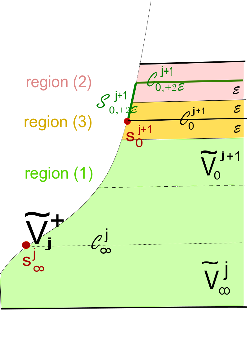
Figure 4.1. The three regions of $\tilde{V}_{j}^{+}$ with respect to the critical line $\mathcal{C}_{0}^{j+1}$ of integration, and the critical points $s_{0}^{j+1},\,s_{\infty}^{j}\in\tilde{V}_{j}^{+}$ generating logarithmic singularities in the proof of Lemma 7.4.

Remark 4.3 (Regions $(1)$, $(2)$, $(3)$ introduced in (LABEL:eq:redi)).

The functions $\tilde{R}_{j,+}^{n},\ n\in\mathbb{N},$ in our iterative process are defined as infinite sums of Cauchy-Heine integrals on corresponding petals $V_{j}^{\pm}$, similarly as in (LABEL:eq:ch) and (3.14). In every step we use another exponentially small cocycle defined from functions obtained in the previous step. Note that functions $\tilde{R}_{j}^{\pm}$ in (3.14) cannot be expressed by the same formula throughout the whole petal $\tilde{V}_{j}^{\pm}$, since integrals are not well-defined along two critical lines of integration that fall inside each petal. Recall that, standardly, in the Cauchy-Heine construction, to extend the function analytically beyond the line of integration, we change the paths of integration, as in the proof of Lemma 3.3.

Each petal $\tilde{V}_{j}^{\pm}$ in $\zeta$-chart is divided into horizontal strip-like regions (sectors in $z$-variable). In each region, we have an explicit, but different integral formula.

We take $\varepsilon>0$ small. Take petal $V_{j}^{+}$. The region $(3)$ is the open $\varepsilon$-neighborhood of two critical lines $\mathcal{C}_{0}^{j+1}$ and $\mathcal{C}_{\infty}^{j}$. These two lines are among the lines of integration in (3.14) for $V_{j}^{+}$, and analogously later in the iterative construction given by (4.11). At the same time, they lie inside $\tilde{V}_{j}^{+}$. The problem in this region is that, although we may exchange the line of integration with a line outside the region and a part of the boundary (here: $\mathcal{C}_{0,+2\varepsilon}^{j+1}$ and $\mathcal{S}_{0,+2\varepsilon}^{j+1}$), we cannot bound the variable $\zeta\in\tilde{V}_{j}^{+}$ away from the part of the boundary, and logarithmic singularities appear in iterations at $s_{0}^{j+1}$ and $s_{\infty}^{j}$, see Figure 4.1. This prevents an easy proof of convergence in our iterative process. The other strips of $\tilde{V}_{j}^{+}$ constitute regions $(1)$ and $(2)$, which are simpler to analyze, as there are no logarithmic singularities. In region $(3)$, the bounds that we need for convergence of iterates in the proof of Lemma 7.4 will be significantly more complicated.

Proof of statement $(2)$. At each step of the iterative Cauchy-Heine construction, two logarithmic singularities appear at points $s_{0}^{j+1}$ and $s_{\infty}^{j}$ at the boundary of each petal $V_{j}^{+}$ in region $(3)$, $j\in\mathbb{Z}$. Precisely, they appear at endpoints of $\mathcal{C}_{0}^{j+1}$ and $\mathcal{C}_{\infty}^{j}$ at the boundary of the domain. Therefore, we will not be able to prove that the sequence of iterates $\big{(}\tilde{R}_{j,+}^{n-1}(\zeta)\big{)}_{n}$ is uniformly Cauchy on the whole petal $\tilde{V}_{+}^{j}$. More details about the nature of the singularities can be found in Subection 7.4 in the Appendix. However, by Lemma 4.2, the sequence

(4.13) $$\big{(}e^{2\pi i\tilde{R}_{j,+}^{n}(\zeta)}\big{)}_{n}$$

is uniformly Cauchy on petals $\tilde{V}_{+}^{j}$, $j\in\mathbb{Z}$. By taking the exponential, we have eliminated the logarithmic singularities. It follows from (4.13) that $\big{(}\tilde{R}_{j,+}^{n}(\zeta)\big{)}_{n}$ is uniformly Cauchy on all compact subsets of the petal $\tilde{V}_{+}^{j}$, away from singular points $s_{0}^{j+1}$ and $s_{\infty}^{j}$ with logarithmic singularities, which lie at the boundary of the petal $V_{j}^{+}$. Indeed, note that $e^{2\pi i\tilde{R}_{j,+}^{n}(\zeta)}$ does not vanish in any point $\zeta\in V_{+}^{j}$. By the mean value theorem, writing $\tilde{R}_{j,+}^{n}=\frac{1}{2\pi i}\log(e^{2\pi i\tilde{R}_{j,+}^{n}})$, we have:

$$|\tilde{R}_{j,+}^{n}(\zeta)-\tilde{R}_{j,+}^{n+1}(\zeta)|\leq$$

$$\leq\frac{1}{\sqrt{2}\pi}\sup_{t\in[0,1]}\frac{1}{\big{|}te^{2\pi i\tilde{R}_{j,+}^{n}(\zeta)}+(1-t)e^{2\pi i\tilde{R}_{j,+}^{n+1}(\zeta)}\big{|}}\!\cdot\!|e^{2\pi i\tilde{R}_{j,+}^{n}(\zeta)}-e^{2\pi i\tilde{R}_{j,+}^{n+1}(\zeta)}|,\,\zeta\in\tilde{V}_{j}^{+}.$$

By Lemma 7.4 (1), we get that $\zeta\mapsto\sup_{t\in[0,1]}\frac{1}{\big{|}te^{2\pi i\tilde{R}_{j,+}^{n}(\zeta)}+(1-t)e^{2\pi i\tilde{R}_{j,+}^{n+1}(\zeta)}\big{|}}$ is uniformly bounded on every compact in the petal $\tilde{V}_{j}^{+}$ away from singular points $s_{0}^{j+1}$ and $s_{\infty}^{j}$. We conclude that the sequence $(\tilde{R}_{j,+}^{n})_{n}$ is uniformly Cauchy on every compact in the petal $\tilde{V}_{j}^{+}$. Therefore, by the Weierstrass theorem, it converges to an analytic function $\tilde{R}_{j}^{+}$ on the petal $\tilde{V}_{j}^{+}$, $j\in\mathbb{Z}$. The same can be concluded for $\tilde{R}_{j}^{-}$ on petals $\tilde{V}_{j}^{-}$, $j\in\mathbb{Z}.$

Let us now denote the pointwise limits by $\tilde{R}_{j}^{\pm}$:

$$\tilde{R}_{j}^{\pm}(\zeta):=\lim_{n\to\infty}\tilde{R}_{j,\pm}^{n}(\zeta),\ \tilde{\Psi}_{j}^{\pm}(\zeta):=\tilde{\Psi}_{\mathrm{nf}}(\zeta)+\tilde{R}_{j,\pm}(\zeta),\ \zeta\in\tilde{V}_{\pm}^{j}.$$

That is, returning from the $\zeta$-variable to the original variable $z$, we put:

$$\breve{R}_{j}^{\pm}(\boldsymbol{\ell}):=\tilde{R}_{j}^{\pm}(\boldsymbol{\ell}^{-1}),\ \Psi_{j}^{\pm}(z):=\Psi_{\mathrm{nf}}(z)+\breve{R}_{j}^{\pm}(\boldsymbol{\ell}),\ z\in V_{\pm}^{j},\ j\in\mathbb{Z}.$$

Here, $\Psi_{\mathrm{nf}}(z)$ i.e. $\tilde{\Psi}_{\mathrm{nf}}(\zeta)$ are the Fatou coordinates of $(2,m,\rho)$-model, analytic on whole $\mathcal{R}_{C}$, and given explicitely in (7.1). All functions defined above are analytic on respective petals. Now, passing to the limit in (LABEL:e:pp), we see that $R_{j}^{\pm}(z)$ and thus also $\Psi_{j}^{\pm}(z)$ (since $\Psi_{\mathrm{nf}}(z)$ is analytic on the standard quadratic domain) realize the requested sequence of pairs $(g_{0}^{j},g_{\infty}^{j})_{j\in\mathbb{Z}}$ at intersections of petals, as in (LABEL:eq:pt).

Proof of statement $(3)$. We use the uniform estimate (4.10) for ${}^{n}\tilde{G}_{0,\infty}^{j}(\zeta)$ by $n\in\mathbb{N}$, deduced in the proof of statement $(1)$, and repeat the proof of (3.6) in Proposition 3.1 (see the proof of Lemma 3.5 in the Appendix), but with this uniform estimate. We get that there exists a uniform (in $j$) constant $C>0$ such that, for substrips $\tilde{S}_{j}\subset\tilde{V}_{j}^{\pm}$ centered at line $\{\mathrm{Im}(\zeta)=j\pi\}$ and of the same opening for all $j\in\mathbb{Z}$, the following estimate holds:

(4.14) $$|\tilde{R}_{j,\pm}^{n}(\zeta)|\leq C|\zeta|^{-1},\ \zeta\in\tilde{S}_{j},\ j\in\mathbb{Z},\ n\in\mathbb{N}.$$

Passing to the limit as $n\to\infty$ in (4.14), and returning to the original variable $z=e^{-\zeta}$, statement $(3)$ is proven. $\Box$

4.2. The symmetry of the horn maps and $\mathbb{R}_{+}$-invariance

We have proven in [7, Proposition 9.2] that, for a parabolic generalized Dulac germ $f$, the fact that $f(\mathbb{R}_{+}\cap\mathcal{R}_{C})\subset\mathbb{R}_{+}\cap\mathcal{R}_{C}$ implies the symmetry (1.10) of its analytic moduli. Here, by abuse, $\mathbb{R}_{+}:=\{z\in\mathcal{R}:\,\mathrm{Arg}(z)=0\}$. In general, the converse of [7, Proposition 9.2] does not hold. That is, the symmetry of horn maps of $f$ does not imply $\mathbb{R}_{+}$-invariance of $f$ in general, as Example 1 below shows. Instead, Lemma 4.4 provides a characterization of analytic germs on standard quadratic domains having symmetric sequences of horn maps.

Example 1.

Take $f(z)=z-z^{2}$ on $\mathcal{R}_{C}$. Obviously, $f$ is a simple parabolic generalized Dulac germ and $f(\mathbb{R}_{+})\subseteq\mathbb{R}_{+}$. By [7, Proposition 9.2], since $f$ is $\mathbb{R}_{+}$-invariant, its moduli are symmetric. Take now $\varphi(z)=z+iz^{3}$, and define an analytic germ $f_{1}:=\varphi^{-1}\circ f\circ\varphi$ on $\mathcal{R}_{C}$. Since $\widehat{f}_{1}(z)=z-z^{2}+o(z^{2})$, $f_{1}$ admits the same petals as $f$. By [7, Theorem B], since $\varphi(z)$ is analytic on $\mathcal{R}_{C}$, $f_{1}$ has the same horn maps as $f$. Therefore, the horn maps of $f_{1}$ are symmetric, but $\mathbb{R}_{+}$ is not $f_{1}$-invariant.

We can easily generate more complicated examples by taking an $\mathbb{R}_{+}$-invariant parabolic generalized Dulac germ and by conjugating it by $\varphi(z)=z+o(z)$ which is analytic on a standard quadratic domain, and whose asymptotic expansion $\widehat{\varphi}$ belongs to $\widehat{\mathcal{L}}(\mathbb{C})$, but not to $\widehat{\mathcal{L}}(\mathbb{R})$. Thus the invariance of $\mathbb{R}_{+}$ is not preserved in general.

Indeed, analytic modulus is an invariant of analytically conjugated parabolic germs. On the other hand, having the real axis invariant is obviously not an invariant property under complex changes of coordinates. If one of the germs has the real axis invariant, all analytically conjugated germs also have an invariant real analytic curve through the singularity, but it is not in general the real axis.

Lemma 4.4 (Symmetry of the horn maps).

Let $f$ be an analytic germ on a standard quadratic domain $\mathcal{R}_{C}$ with a sequence of horn maps $(h_{0}^{j},h_{\infty}^{j};\sigma_{j})_{j\in\mathbb{Z}}$, with $\sigma_{j}$ as in (1.8). The sequence of horn maps is symmetric, that is,

(4.15) $$\overline{\big{(}h_{0}^{-j+1}\big{)}^{-1}(t)}\equiv h_{\infty}^{j}(\overline{t}),\ t\in(\mathbb{C},0),\ j\in\mathbb{Z},$$

if and only if there exists an analytic germ $\varphi(z)=z+o(z)$ on $\mathcal{R}_{C}$ such that

(4.16) $$\overline{f(\overline{z})}=\varphi^{-1}\circ f\circ\varphi(z),\ z\in\mathcal{R}_{C}.$$

Note that (4.16) is trivially satisfied for germs $f$ such that $f(\mathbb{R}_{+})\subseteq\mathbb{R}_{+}$, taking $\varphi=\mathrm{id}$, by the Schwarz reflection principle.

Proof.

Let $f$ be analytic on a standard quadratic domain $\mathcal{R}_{C}$. Let $f_{1}(z):=\overline{f(\overline{z})},\ z\in\mathcal{R}_{C}$. It is an analytic function on $\mathcal{R}_{C}$ by the Cauchy-Riemann conditions. Let $(k_{0}^{j},k_{\infty}^{j};\sigma_{j})_{j\in\mathbb{Z}}$ be its sequence of horn maps ($\sigma_{j}$ remains the same, due to symmetry of standard quadratic domains). Then, by the proof of [7, Proposition 9.2], it holds that

(4.17) $$\overline{\big{(}k_{0}^{-j+1}\big{)}^{-1}(t)}\equiv h_{\infty}^{j}(\overline{t}),\ \overline{(k_{\infty}^{j})^{-1}(t)}=h_{0}^{-j+1}(\overline{t}),\ t\in(\mathbb{C},0),\ j\in\mathbb{Z}.$$

By (4.17) and symmetry (4.15) of the horn maps of $f$, we conclude that $f_{1}$ and $f$ have the same sequence of horn maps. By [7, Theorem B], there exists an analytic function $\varphi(z)=z+o(z)$ on $\mathcal{R}_{C}$ such that

$$\overline{f(\overline{z})}=\varphi^{-1}\circ f\circ\varphi(z),\ z\in\mathcal{R}_{C}.$$

The other direction is proven similarly. ∎

However, in Lemma 4.5 we show that, if we take a symmetric sequence of pairs of analytic germs from $\mathrm{Diff}(\mathbb{C},0)$, by Cauchy-Heine construction from Lemma 4.1 we realize the sequence by a representative that is indeed $\mathbb{R}_{+}$-invariant, as its horn maps. The reason lies in the symmetry of the Cauchy-Heine construction.

Lemma 4.5.

Let $(h_{0}^{j},h_{\infty}^{j};\sigma_{j})_{j\in\mathbb{Z}}$, with $\sigma_{j}$ as in (1.8), be a symmetric sequence of pairs of analytic germs from $\mathrm{Diff}(\mathbb{C},0)$, such that:

(4.18) $$\overline{\big{(}h_{0}^{-j+1}\big{)}^{-1}(t)}\equiv h_{\infty}^{j}(\overline{t}),\ t\in(\mathbb{C},0),\ j\in\mathbb{Z}.$$

Let $\Psi_{j}^{\pm}(z):=\Psi_{\mathrm{nf}}+\breve{R}_{j}^{\pm}(\boldsymbol{\ell})$, $\breve{R}_{j}^{\pm}(\boldsymbol{\ell}):=R_{j}^{\pm}(z)$, $z\in V_{j}^{\pm}$, be as constructed by the iterative Cauchy-Heine construction in Lemma 4.1, realizing the sequence of pairs $(h_{0}^{j},h_{\infty}^{j};\sigma_{j})_{j\in\mathbb{Z}}$ on intersections of petals $V_{0}^{j},\ V_{\infty}^{j},\ j\in\mathbb{Z}$, either on a standard linear or a standard quadratic domain. Then:

1. $\Psi_{0}^{+}$ on $V_{0}^{+}$ is $\mathbb{R}_{+}$-invariant. That is,

   $$\Psi_{0}^{+}(\mathbb{R}_{+}\cap\mathcal{R}_{C})\subseteq\mathbb{R}_{+}\cap\mathcal{R}_{C}\text{\ \ $($resp. $\mathcal{R}_{a,b}$$)$}.$$

2. In the case of construction on a standard linear domain, the asymptotic expansion $\widehat{R}(\boldsymbol{\ell})$ of $\breve{R}_{j}^{\pm}(\boldsymbol{\ell})$, as $\boldsymbol{\ell}\to 0$ on $\boldsymbol{\ell}$-cusps $\boldsymbol{\ell}(V_{j}^{\pm})$, belongs to $\mathbb{R}[[\boldsymbol{\ell}]]$. That is, the coefficients of the expansion are real.

The proof is in the Appendix.

4.3. Proof of Theorem A

Proof.

Let $(h_{0}^{j},h_{\infty}^{j};\,\sigma_{j})_{j\in\mathbb{Z}}$ be a sequence of pairs of analytic germs of diffeomorphisms, as in Theorem A. Let $V_{j}^{\pm}$ be the petals of opening $2\pi$, centered at $j\pi$, $j\in\mathbb{Z}$, along a standard quadratic domain, as in Figure 1.4. By Lemma 4.1, we construct analytic functions $\Psi_{j}^{\pm}$ on $V_{j}^{\pm}$ that satisfy (LABEL:eq:pt). This is equivalent to the relation (LABEL:eq:moduli) for the realization of horn maps. We now define $f$ such that $\Psi_{j}^{\pm}$ are its petalwise Fatou coordinates. We define $f$ by petals, using Abel equation, as:

(4.19) $$f_{j}^{\pm}(z):=(\Psi_{j}^{\pm})^{-1}(1+\Psi_{j}^{\pm}(z)),\ z\in V_{j}^{\pm},\ j\in\mathbb{Z}.$$

Now we prove that $f_{j}^{\pm}$, defined and analytic on petals $V_{j}^{\pm}$, glue to an analytic function $f$ on the whole standard quadratic domain $\mathcal{R}_{C}$. That is, we prove that

(4.20) $$\begin{split}&f_{j}^{+}(z)=f_{j}^{-}(z),\ z\in V_{\infty}^{j}=V_{+}^{j}\cap V_{-}^{j},\\ &f_{j-1}^{+}(z)=f_{j}^{-}(z),\ z\in V_{0}^{j}=V_{j-1}^{+}\cap V_{j}^{-},\ j\in\mathbb{Z}.\end{split}$$

Indeed, for Fatou coordinates $\Psi_{j}^{\pm}$ of two consecutive petals by (LABEL:eq:pt) of Lemma 4.1 it holds that:

$$\Psi_{-}^{j}\circ(\Psi_{+}^{j-1})^{-1}(w)=w-g_{0}^{j}(e^{-2\pi iw}),\ w\in\Psi_{+}^{j-1}(V_{0}^{j}),$$

$$\Psi_{-}^{j}\circ(\Psi_{+}^{j})^{-1}(w)=w+g_{\infty}^{j}(e^{2\pi iw}),\ w\in\Psi_{+}^{j}(V_{\infty}^{j}),\ j\in\mathbb{Z}.$$

This implies:

$$\Psi_{-}^{j}\circ(\Psi_{+}^{j-1})^{-1}(w+1)=\Psi_{-}^{j}\circ(\Psi_{+}^{j-1})^{-1}(w)+1,\ w\in\Psi_{+}^{j-1}(V_{0}^{j}),$$

$$\Psi_{-}^{j}\circ(\Psi_{+}^{j})^{-1}(w+1)=\Psi_{-}^{j}\circ(\Psi_{+}^{j})^{-1}(w)+1,\ w\in\Psi_{+}^{j}(V_{\infty}^{j}),\ j\in\mathbb{Z}.$$

Composing the first equation by $\Psi_{+}^{j-1}$ from the right and by $(\Psi_{-}^{j})^{-1}$ from the left, and the second by $\Psi_{+}^{j}$ from the right and $(\Psi_{-}^{j})^{-1}$ from the left, by (4.19) we get (LABEL:eq:treba).

The prenormalized form (2.7) of $f$ follows from Proposition 7.1 in the Appendix and the prenormalized form of the Fatou coordinates $\Psi_{j}^{\pm}=\Psi_{\mathrm{nf}}+R_{j}^{\pm}$ constructed in Lemma 4.1. Here, $R_{j}^{\pm}(z)=o(1)$, as $z\to 0$ on $V_{j}^{\pm}$, and $\Psi_{\mathrm{nf}}$ is the Fatou coordinate of $(2,m,\rho)$-formal model.

The uniform bound $|f(z)-z+z^{2}\boldsymbol{\ell}^{m}-\rho z^{3}\boldsymbol{\ell}^{2m+1}|\leq C|z^{3}\boldsymbol{\ell}^{2m+2}|,\ C>0,\ z\in\mathcal{R}_{c}$, follows by Lemma 4.1 (3). Indeed, uniform bound (4.6) gives that there exists $d>0$, independent of $j\in\mathbb{Z}$, such that $|\Psi_{j}^{\pm}(z)-\Psi_{\mathrm{nf}}(z)|\leq d|\boldsymbol{\ell}|,\ z\in S_{j}\subset V_{j}^{\pm}$, where $S_{j}^{\pm}$ are subsectors of $V_{j}^{\pm}$ of the same opening strictly bigger than $\pi$ for all $j\in\mathbb{Z}$. The same reasoning as in the proof of Proposition 7.1 in the Appendix now gives the bound $|f(z)-f_{0}(z)|\leq e|z^{3}\boldsymbol{\ell}^{2m+2}|,\ z\in\mathcal{R}_{c},\ e>0$. Then, using uniform bound for the model, $|f_{0}(z)-z+z^{2}\boldsymbol{\ell}^{m}-\rho z^{3}\boldsymbol{\ell}^{2m+1}|\leq c_{1}|z^{3}\boldsymbol{\ell}^{2m+2}|,\ z\in\mathcal{R}_{c}$, $c_{1}>0$, we get the required bound for $f$.

Finally, on $V_{0}^{+}$ the germ $f$ is given by

(4.21) $$f\Big{|}_{V_{0}^{+}}\Big{.}=(\Psi_{0}^{+})^{-1}(1+\Psi_{0}^{+}),$$

and glues analytically along other petals. By Lemma 4.5, $\Psi_{0}^{+}$ is $\mathbb{R}_{+}$-invariant. It is also injective on $\mathbb{R}_{+}\cap V_{0}^{+}$, so the inverse $(\Psi_{0}^{+})^{-1}$ is $\mathbb{R}_{+}$-invariant on $\Psi_{0}^{+}(V_{0}^{+})$. We conclude by (4.21) that $f$ is $\mathbb{R}_{+}$-invariant. ∎

5. Proof of Theorem B

The analogue of Lemma 4.1 holds (with the same proof) also on standard linear domains. Given a sequence of pairs of analytic germs of diffeomorphisms $(h_{0}^{j},h_{\infty}^{j};\sigma_{j})_{j\in\mathbb{Z}}$, with radii of convergence satisfying bounds (1.11), we construct analytic functions $\Psi_{j}^{\pm}(z)$ on petals $V_{j}^{\pm}$ centered at directions $2j\pi$ (attracting), that is, $(2j-1)\pi$ (repelling), but along a standard linear domain, that realize this sequence of diffeomorphisms on intersections of petals $V_{0,\infty}^{j}$, as in (LABEL:eq:pt). We construct them as the uniform limits $R_{j}^{\pm}$ on compact subsets of $V_{j}^{\pm}$ of iterates $R_{j,\pm}^{n}(z)$, as $n\to\infty$, defined inductively as in Lemma 4.1. In each inductive step, we use Proposition 3.2 for realization of cocycles on standard linear domains, instead of Proposition 3.1 for standard quadratic domains. Proposition 3.2 additionaly gives us information on asymptotic expansion of $R_{j,\pm}^{n}$, $n\in\mathbb{N}$. Let $\breve{R}_{j,\pm}^{n}(\boldsymbol{\ell}):=R_{j,\pm}^{n}(z),\ z\in V_{j}^{\pm}$, where $\boldsymbol{\ell}:=-\frac{1}{\log z}$. Then, by Proposition 3.2, each $R_{j,\pm}^{n}(\boldsymbol{\ell})$, $j\in\mathbb{Z}$, admits $\log$-Gevrey expansion in $\mathbb{C}[[\boldsymbol{\ell}]]$ of every order $1-\delta$, $\delta>0$, as $\boldsymbol{\ell}\to 0$ in $\boldsymbol{\ell}(V_{j}^{\pm})$.

We now prove that there exists $\widehat{R}(\boldsymbol{\ell})\in\mathbb{C}[[\boldsymbol{\ell}]]$ such that the limits

$$\breve{R}_{j}^{\pm}(\boldsymbol{\ell}):=\lim_{n\to\infty}\breve{R}_{j,\pm}^{n}(\boldsymbol{\ell}),\ \boldsymbol{\ell}\in\boldsymbol{\ell}(V_{j}^{\pm}),\ j\in\mathbb{Z},$$

admit $\widehat{R}(\boldsymbol{\ell})$ as their $\log$-Gevrey asymptotic expansion of order $1-\delta$, for every $\delta>0$, as $\boldsymbol{\ell}\to 0$ on $\boldsymbol{\ell}(V_{j}^{\pm})$. Moreover, we prove that $\widehat{R}(\boldsymbol{\ell})\in\mathbb{R}[[\boldsymbol{\ell}]]$.

We work again in the logarithmic chart $\zeta=-\log z$. As in the proof of Lemma 3.5 in the Appendix, on standard linear domains it follows that:

$$\Big{|}\sum_{k=j+1}^{+\infty}{}^{n}\tilde{F}_{0,k}^{-}(\zeta)-\sum_{j=0}^{N}a_{j}^{n}\zeta^{-j}\Big{|}\leq$$

$$\ \ \leq|\zeta|^{-N}\frac{1}{2\pi}\sum_{k=j+1}^{+\infty}\Big{|}\int_{\mathcal{C}_{0}^{k}}\frac{g_{0}^{k}(e^{-2\pi i(\tilde{\Psi}_{\mathrm{nf}}(w)+\tilde{R}_{k-1,+}^{n-1}(w))})w^{N}}{w-\zeta}\,dw\Big{|},$$

$$\qquad\qquad\qquad\qquad\qquad\qquad\qquad\qquad\qquad\qquad\zeta\in\tilde{V}_{j}^{+}\text{ in the region (1)},\ N\in\mathbb{N}.$$

Here we again consider, instead of the whole $\tilde{R}_{j,+}^{n}(\zeta)$ given by (4.11), only one part of the sum $\sum_{k=j+1}^{+\infty}{}^{n}\tilde{F}_{0,k}^{-}(\zeta),\ \zeta\in\tilde{V}_{j}^{+}$, see (LABEL:eq:redi). For the other three parts of the sum the conclusions follow similarly. To get the bound for $\tilde{R}_{j,+}^{n}(\zeta)$, we sum the bounds afterwards. Additionally, for $\zeta\in\tilde{V}_{j}^{+}$ in regions (2) and (3), the conclusion follows similarly. Finally, the same can be done for $\tilde{R}_{j,-}^{n}$ on $\tilde{V}_{j}^{-}$. Let $\delta>0$. Due to uniform bounds of $g_{0}^{k}$ from (2.5) and of $\tilde{R}_{k,+}^{n}$ (see Remark 7.5) with respect to $n\in\mathbb{N}$ and $k\in\mathbb{Z}$, we conclude that there exist uniform constants $c>0$ and $d>0$, such that:

(5.1) $$\big{|}g_{0}^{k}(e^{-2\pi i(\tilde{\Psi}_{\mathrm{nf}}(w)+\tilde{R}_{k-1,+}^{n-1}(w))})\big{|}\!\!<\!c|e^{-2\pi i(\tilde{\Psi}_{\mathrm{nf}}(w)+\tilde{R}_{k-1,+}^{n-1}(w))}|\!<\!d|e^{-2\pi i(\tilde{\Psi}_{\mathrm{nf}}(w)/2)}|,\ w\in V_{0}^{k},$$

for every $n\in\mathbb{N}$ and $k\in\mathbb{Z}$.

Now, following the proof of Lemma 3.5 in the Appendix and using (5.1), we obtain Gevrey bounds which are uniform with respect to $n\in\mathbb{N}$. That is, on every substrip $\tilde{W}\subset\tilde{V}_{j}^{+}$, for every $N\in\mathbb{N}$, there exists a constant $C_{N}^{\tilde{W}}>0$ such that, for every $n\in\mathbb{N}$, it holds that:

(5.2) $$|\tilde{R}_{j,+}^{n}(\zeta)-\sum_{i=0}^{N}A_{i}^{j,n}\zeta^{-i}|\leq C_{N}^{\tilde{W}}(1-\delta)^{-N}e^{-\frac{N}{\log N}}\log^{N}N\cdot|\zeta|^{-N},\ \zeta\in\tilde{W}\subset\tilde{V}_{j}^{+}.$$

Here, $C_{N}^{\tilde{W}}$ is uniform in the iterate $n\in\mathbb{N}$. Also, $A_{i}^{j,n}\in\mathbb{C}$ is given by:

$$A_{i}^{j,n}:=\sum_{k=j+1}^{\infty}\int_{\mathcal{C}_{0}^{k}}g_{0}^{k}(e^{-2\pi i(\tilde{\Psi}_{\mathrm{nf}}w)+\tilde{R}_{k-1,+}^{n-1}(w))})w^{i}\,dw.$$

As discussed before in the proof of Lemma 3.5, the above sum converges for every $n\in\mathbb{N},\,j\in\mathbb{Z}$, so the coefficients $A_{i}^{j,n}\in\mathbb{C}$ are well-defined. To prove that, for every $j\in\mathbb{Z}$, $i\in\mathbb{N}_{0}$, $(A_{i}^{j,n})_{n}$ converges as $n\to\infty$, we use the dominated convergence theorem. Indeed, by a change of variable of integration, the above integrals $\int_{\mathcal{C}_{0}^{k}}$ can be considered as line integrals. Now (5.1) and the convergence of the following integrals:

$$\int_{\mathcal{C}_{0}^{k}}|e^{-2\pi i(\tilde{\Psi}_{\mathrm{nf}}(w)/2)}|w^{i}\,dw,\ k\in\mathbb{Z},$$

due to the exponential flatness of $e^{-2\pi i(\tilde{\Psi}_{\mathrm{nf}}(w)/2)}$ on $\mathcal{C}_{0}^{k}$, $k\in\mathbb{Z}$, ensures all the assumptions of the dominated convergence theorem. We put:

$$A_{i}^{j}:=\lim_{n\to\infty}A_{i}^{j,n}\,\in\mathbb{C},\ j\in\mathbb{Z},\ i\in\mathbb{N}_{0}.$$

Now passing to the limit $\lim_{n\to\infty}$ in (5.2), we get that $\tilde{R}_{j}^{+}(\zeta):=\lim_{n\to\infty}\tilde{R}_{j,+}^{n}(\zeta)$, $\zeta\in\tilde{V}_{j}^{+},$ admits a $\log$-Gevrey asymptotic expansion of order $1-\delta$ in $\mathbb{C}[[\zeta^{-1}]]$, as $\mathrm{Re}(\zeta)\to\infty$.

In addition, the asymptotic expansions of $\tilde{R}_{j}^{\pm}(\zeta)$ are the same for every $j\in\mathbb{Z}$, because of exponentially small differences on intersections of petals (LABEL:eq:pt). Recall that $\tilde{\Psi}_{j}^{\pm}:=\tilde{\Psi}_{\mathrm{nf}}+\tilde{R}_{j}^{\pm}$ on $\tilde{V}_{j}^{\pm}$, where $\tilde{\Psi}_{\mathrm{nf}}$ is globally analytic on a standard quadratic domain. We denote this expansion by $\widehat{R}(\zeta^{-1})\in\mathbb{C}[[\zeta^{-1}]]$. That is, putting $\boldsymbol{\ell}:=\zeta^{-1}=-\frac{1}{\log z}$, all $\breve{R}_{j}^{\pm}(\boldsymbol{\ell}):=\tilde{R}_{j}^{\pm}(\zeta)$ admit $\widehat{R}(\boldsymbol{\ell})$, as their $\log$-Gevrey asymptotic expansion of order $1-\delta$, as $\boldsymbol{\ell}\to 0$ on $\boldsymbol{\ell}(V_{j}^{\pm})$, $j\in\mathbb{Z}$.

Finally, we prove that $f$, expressed as in (4.19) from $\tilde{\Psi}_{j}^{\pm}$, and which, by the proof of Theorem A, glues to an analytic function on a standard linear domain $\widetilde{\mathcal{R}}_{a,b}$, is a parabolic generalized Dulac germ. The uniform bound (2.3) and the prenormalized form of $f$ follow from Lemma 4.1 (3) and by Proposition 7.1 in the Appendix, exactly as in the proof of Theorem A. Also, the invariance of $\mathbb{R}_{+}$ follows by Lemma 4.5, as in the proof of Theorem A.

We prove only the existence of the generalized Dulac expansion $\widehat{f}$ of $f$. It follows by (4.19) and by the $\log$-Gevrey asymptotic expansions of $\breve{R}_{j}^{\pm}(\boldsymbol{\ell})\text{ on }\boldsymbol{\ell}(V_{j}^{\pm}),\ j\in\mathbb{Z}$, proven above. We return to the original variable $z$. On each petal $V_{j}^{\pm}$, we expand (4.19) in Taylor expansion:

(5.3) $$f_{j}^{\pm}(z)=z+\frac{1}{(\Psi_{j}^{\pm})^{\prime}(z)}+\frac{1}{2!}\Big{(}\frac{1}{(\Psi_{j}^{\pm})^{\prime}(z)}\Big{)}^{\prime}\cdot\frac{1}{(\Psi_{j}^{\pm})^{\prime}(z)}+\frac{1}{3!}(\textrm{previous\ term})^{\prime}\cdot\frac{1}{(\Psi_{j}^{\pm})^{\prime}(z)}+\ldots$$

In the sequel, we put $\breve{R}_{j}^{\pm}(\boldsymbol{\ell}):=R_{j}^{\pm}(z),\ z\in V_{j}^{\pm}$. Let $\widehat{R}(\boldsymbol{\ell})$ denote its $\log$-Gevrey asymptotic expansion of order $1-\delta$, $\delta>0$, in $\mathbb{C}[[\boldsymbol{\ell}]]$, the same for all $j\in\mathbb{Z}$. It holds:

$$(\Psi_{j}^{\pm})^{\prime}(z)=-\frac{1}{z^{2}\boldsymbol{\ell}^{m}}+\frac{1}{z}+\big{(}\frac{m}{2}+\rho\big{)}\frac{\boldsymbol{\ell}}{z}+\frac{\boldsymbol{\ell}^{2}}{z}(\breve{R}_{j}^{\pm})^{\prime}(\boldsymbol{\ell}),\ \rho\in\mathbb{R},\ m\in\mathbb{Z},\ z\in V_{j}^{\pm}.$$

Here, the germs $(\breve{R}_{j}^{\pm})^{\prime}(\boldsymbol{\ell})$ are analytic on $\boldsymbol{\ell}$-cusps $\boldsymbol{\ell}(V_{j}^{\pm})$, $j\in\mathbb{Z}$. By [7, Proposition 4.7], they expand $\log$-Gevrey of order $1-\delta$, for every $\delta>0$, in their formal counterpart $\widehat{R}^{\prime}(\boldsymbol{\ell})$, as $\boldsymbol{\ell}\to 0$ on $\boldsymbol{\ell}$-cusp $\boldsymbol{\ell}(V_{j}^{\pm})$. By [7, Proposition 4.7], $\widehat{R}^{\prime}(\boldsymbol{\ell})$ is obtained by termwise (formal) derivation of $\widehat{R}(\boldsymbol{\ell})$. The same conclusion can be drawn for all finite derivatives $(\breve{R}_{j}^{\pm})^{(k)}(\boldsymbol{\ell})$, $k\in\mathbb{N}$, by [7, Proposition 4.7]. Furthermore, we define analytic functions $H_{j}^{\pm}(\boldsymbol{\ell})$ on $\boldsymbol{\ell}$-cusps $\boldsymbol{\ell}(V_{j}^{\pm})$, $j\in\mathbb{Z}$, through the following equation:

$$\frac{1}{(\Psi_{j}^{\pm})^{\prime}(z)}=\frac{-z^{2}\boldsymbol{\ell}^{m}}{1-z\boldsymbol{\ell}^{m}-(\frac{m}{2}+\rho)z\boldsymbol{\ell}^{m+1}+z\boldsymbol{\ell}^{m+2}(\breve{R}_{j}^{\pm})^{\prime}(\boldsymbol{\ell})}=:\frac{-z^{2}\boldsymbol{\ell}^{m}}{1+zH_{j}^{\pm}(\boldsymbol{\ell})}.$$

By [7, Propositions 4.5-4.7] about closedness of $\log$-Gevrey classes to algebraic operations and to differentiation, they expand $\log$-Gevrey of order $1-\delta$, for every $\delta>0$, in the common formal counterpart $\widehat{H}(\boldsymbol{\ell})$, as $\boldsymbol{\ell}\to 0$ on respective $\boldsymbol{\ell}$-cusps $\boldsymbol{\ell}(V_{j}^{\pm})$, $j\in\mathbb{Z}$. Note that

(5.4) $$\frac{z^{2}\boldsymbol{\ell}^{m}}{1+zH_{j}^{\pm}(\boldsymbol{\ell})}=z^{2}\boldsymbol{\ell}^{m}\sum_{k=0}^{\infty}(-1)^{k}z^{k}(H_{j}^{\pm}(\boldsymbol{\ell}))^{k}.$$

Putting (5.4) in (5.3), and regrouping the terms with the same powers of $z$, we get:

(5.5) $$f(z)=z-z^{2}\boldsymbol{\ell}^{m}+\rho z^{3}\boldsymbol{\ell}^{2m+1}+\sum_{k=3}^{\infty}z^{k}Q_{j,k}^{\pm}(\boldsymbol{\ell}),\ z\in V_{j}^{\pm},\ j\in\mathbb{Z}.$$

Here, $Q_{j,k}^{\pm}(\boldsymbol{\ell})$, $k\in\mathbb{N}$, $k\geq 3$, are realized as finite sums of finite products of $\boldsymbol{\ell}$ and $H_{j}^{\pm}(\boldsymbol{\ell})$ and their finite derivatives (of order at most $k-2$), the same for all petals $j\in\mathbb{Z}$. Therefore, by [7, Propositions 4.5-4.7] about closedness of $\log$-Gevrey classes to algebraic operations and differentiation, they expand $\log$-Gevrey of order $1-\delta$, for every $\delta>0$, in their formal counterpart, denoted $\widehat{Q}_{k}(\boldsymbol{\ell})$. Note that $\boldsymbol{\ell}$-cusps $\boldsymbol{\ell}(V_{j}^{\pm})$ are $\boldsymbol{\ell}$-images of sectors of opening $2\pi>\pi$.

Finally, by Lemma 4.5 (b), $\widehat{R}(\boldsymbol{\ell})\in\mathbb{R}[[\boldsymbol{\ell}]]$. Therefore, all $\widehat{Q}_{k}(\boldsymbol{\ell})$, as algebraic combinations of $\widehat{R}(\boldsymbol{\ell})$, its derivatives and powers of $\boldsymbol{\ell}$ with real coefficients, belong to $\mathbb{R}[[\boldsymbol{\ell}]]$. This proves the generalized Dulac expansion of $f$ from Definition 1.4. $\Box$

In Remark 7.3 in the Appendix we explain why the arguments giving the asymptotic expansion in Theorem B do not work for quadratic domains in Theorem A.

Remark 5.1.

Note that, although $f$ is analytic on the whole standard linear domain $\mathcal{R}_{a,b}$, the coefficient functions $Q_{j,k}^{\pm}(\boldsymbol{\ell})$, $k\in\mathbb{N},\ k\geq 3$, in its expansion (5.5) are analytic in general only on $\boldsymbol{\ell}$-cusps $\boldsymbol{\ell}(V_{j}^{\pm})$ and do not glue (in $j$) to an analytic function on whole $\boldsymbol{\ell}(\mathcal{R}_{a,b})$. Indeed, this is obviously not true already for $Q_{j,3}^{\pm}(\boldsymbol{\ell}):=1-H_{j}^{\pm}(\boldsymbol{\ell})$, by (5.4). On overlapping cusps $\boldsymbol{\ell}(V_{j}^{\pm})$, the $\boldsymbol{\ell}$-images of petals $V_{j}^{\pm}$, they have exponentially small differences.

Remark 5.2.

Let the germs $f$ resp. $g$ be the germs obtained by Cauchy-Heine construction on a linear resp. quadratic domain realizing the same sequence of moduli. It is important to note that, in general, $f$ is not the restriction of the germ $g$, since we apply Cauchy-Heine integrals along different lines, see Remark 3.6.

Nevertheless, $f$ and the restriction of $g$ to a linear domain by construction have the same moduli on the linear domain, and are thus analytically conjugated on the linear domain. However, we are not sure if the analytic conjugacy between the two germs on the linear domain can be analytically extended to a quadratic domain, or if there is some singularity outside the smaller domain preventing the extension. If former was the case, we would have a representative of the analytic class of $g$ on a quadratic domain whose restriction to the linear domain is $f$; that is, a representative with the generalized Dulac asymptotic expansion. This would positively resolve the question of extending the realization result to parabolic Dulac germs on a standard quadratic domain, which for the moment remains open.

6. Prospects.

The realization Theorem B for uniformly bounded sequences of pairs of germs of analytic diffeomorphisms fixing the origin as horn maps is proven in the larger class of parabolic generalized Dulac germs on standard linear domains, that contains parabolic Dulac germs. The question if the construction can be extended to standard quadratic domains remains open. Another important problem is to characterize uniformly bounded sequences of pairs of analytic diffeomorphisms which can be realized as horn maps of parabolic Dulac germs.

7. Appendix

Proposition 7.1.

Let $f$ be a parabolic generalized Dulac germ on a standard quadratic (or standard linear) domain. It is prenormalized, that is, of the form:

$$f(z)=z-z^{2}\boldsymbol{\ell}^{m}+\rho z^{3}\boldsymbol{\ell}^{2m+1}+o(z^{2}\boldsymbol{\ell}^{m}),\ m\in\mathbb{Z},\ \rho\in\mathbb{R},$$

if and only if its sectorial Fatou coordinate is of the form:

$$\Psi_{j}^{\pm}=\Psi_{\mathrm{nf}}+R_{j}^{\pm},\text{ on }V_{j}^{\pm},$$

where $R_{j}=o(1)$, as $z\to 0,\ z\in V_{j}^{\pm}$, and $\Psi_{\mathrm{nf}}$ is the global Fatou coordinate of the formal normal form $f_{0}$ given by:

(7.1) $$\Psi_{\mathrm{nf}}(z):=-\int_{z_{0}}^{z}\frac{dz}{z^{2}\boldsymbol{\ell}^{m}}+\log z-(\frac{m}{2}+\rho)\log(-\log z).$$

Here, $z_{0}$ is a freely chosen initial point in the standard quadratic $($or linear$)$ domain $($the choice of additive constant in $\Psi_{\mathrm{nf}})$.

Proof.

One direction is proven by Taylor expansion of the Abel equation. For the other, putting $f=f_{0}+h$ and $\Psi_{j}^{\pm}=\Psi_{\mathrm{nf}}+R_{j}^{\pm}$ in $f=(\Psi_{j}^{\pm})^{-1}(1+\Psi_{j}^{\pm})$ and comparing initial terms, we estimate $h(z)=O(z^{3}\boldsymbol{\ell}^{2m+2})$, as $z\to 0$. The estimate is not necessarily uniform for all petals. ∎

7.1. Proof of Proposition 2.1

In the proof of Proposition 2.1, we use Lemma 7.2.

Lemma 7.2 (Uniform bound on the Fatou coordinate of a uniformly bounded germ).

Let $f(z)=z-z^{2}\boldsymbol{\ell}^{m}+\rho z^{3}\boldsymbol{\ell}^{2m+1}+o(z^{3}\boldsymbol{\ell}^{2m+1}),\ m\in\mathbb{Z},\ \rho\in\mathbb{R},$ be a prenormalized analytic germ on a standard quadratic or standard linear domain $\mathcal{R}_{c}$. Let $f$ satisfy the uniform bound (2.3). Let $\Psi_{\mathrm{nf}}(z)$, $z\in\mathcal{R}_{c}$, be the Fatou coordinate of the formal $(2,m,\rho)$-normal form $f_{0}$ defined in (7.1). Then, for every $0<\theta<2\pi$, there exists a constant $C_{\theta}>0$, such that, for all subsectors $W_{\theta}^{j}\subset V_{j}^{\pm}$ of opening $0<\theta<2\pi$, $j\in\mathbb{Z}$, it holds that:

(7.2) $$|\Psi_{j}^{\pm}(z)-\Psi_{\mathrm{nf}}(z)|\leq C_{\theta}\boldsymbol{\ell}(|z|),\ z\in W_{\theta}^{j}\subset V_{j}^{\pm}.$$

Proof.

The proof is divided in two steps. In Step 1, we show a uniform bound on $|\Psi_{\mathrm{nf}}(z)|$ on a standard quadratic (linear) domain. In Step 2, using this bound, we prove (7.2).

Step 1. Using the explicit form (7.1) of $\Psi_{\mathrm{nf}}$, we prove that there exists $C>0$ such that:

(7.3) $$|\Psi_{\mathrm{nf}}(z)|\leq C|z^{-1}\boldsymbol{\ell}^{-m}|,\ z\in\mathcal{R}_{c}.$$

In the course of the proof, we will pass to a smaller standard quadratic subdomain whenever needed, because we work with germs. Note that, for every $(\alpha,m)\prec(\beta,k)$, there exists a constant $C$ and a sufficiently small standard quadratic domain $\mathcal{R}_{c}$ such that $|z^{\beta}\boldsymbol{\ell}^{k}|\leq C|z^{\alpha}\boldsymbol{\ell}^{m}|,\ z\in\mathcal{R}_{c}$. Note also that this is not the case for the whole Riemann surface of the logarithm of sufficiently small radius.

By two partial integrations, we get, up to a constant term:

(7.4) $$\big{|}\Psi_{\mathrm{nf}} (z)-z^{-1}\boldsymbol{\ell}^{-m}+mz^{-1}\boldsymbol{\ell}^{-m+1}\big{|}=$$

$$=\Big{|}-m(m-1)\int_{z_{0}}^{z}z^{-2}\boldsymbol{\ell}^{-m+2}+\log z-(\frac{m}{2}+\rho)\log(-\log z)\Big{|}\leq$$

$$\leq|m|\,|m-1|\cdot|G(z)-G(z_{0})|+|\boldsymbol{\ell}^{-1}|+\Big{|}\frac{m}{2}+\rho\Big{|}\cdot\big{|}\log(-\log z)\big{|}\leq$$

$$\leq C\Big{(}|G(z)|+|\boldsymbol{\ell}^{-1}|+|\boldsymbol{\ell}_{2}^{-1}|\Big{)},\ z\in\mathcal{R}_{c}.$$

Here, $z_{0}\in\mathcal{R}_{c}$ is fixed, and $G(z)$ denotes the primitive function, such that $G^{\prime}(z)=z^{-2}\boldsymbol{\ell}^{-m+2}$. We prove now that there exists a constant $d>0$ such that:

$$|G(z)|\leq d\,|z^{-1}\boldsymbol{\ell}^{-m+2}|,\ z\in\mathcal{R}_{c}.$$

We pass to the logarithmic chart $\zeta=-\log z$ and put $H(\zeta):=G(e^{-\zeta})$. Then $H^{\prime}(\zeta)=-e^{\zeta}\zeta^{m-2}$. Let $\zeta_{0}:=-\log z_{0}$ be fixed. We may take e.g. $\zeta_{0}\in\mathbb{R}_{+}$. Let $\gamma_{\zeta}$ be the rectangular path from $\zeta_{0}$ to $\zeta$, $\zeta\in\widetilde{\mathcal{R}}_{c}$, consisting of horizontal segment $[\zeta_{0},\zeta_{1}]$ and vertical segment $[\zeta_{1},\zeta]$. Then:

$$H(\zeta)-H(\zeta_{0})=\int_{\gamma_{\zeta}}H^{\prime}(\eta)d\eta,\ \zeta\in\widetilde{\mathcal{R}}_{c}.$$

Evidently, the integral depends only on $\zeta_{0}$ and $\zeta$, and not on the integration path, since $\widetilde{\mathcal{R}}_{c}$ is simply connected. We integrate partially $r-2$ times, where $r$ is such that $m-r<0$, and get:

(7.5) $$\begin{split}&|G(z)-G(z_{0})|=|H(\zeta)-H(\zeta_{0})|=\\ &=\Big{|}\int_{\zeta_{0}}^{\zeta_{1}}e^{\eta}\eta^{m-r}d\eta+\int_{\zeta_{1}}^{\zeta}e^{\eta}\eta^{m-r}d\eta+c_{m-2}e^{\zeta}\zeta^{m-2}+\dots+c_{m-r+1}e^{\zeta}\zeta^{m-r+1}-H(\zeta_{0})\Big{|}\\ &\leq|H(\zeta_{0})|+|c_{m-2}||e^{\zeta}||\zeta|^{m-2}+\ldots+|c_{m-r+1}||e^{\zeta}||\zeta|^{m-r+1}+\\ &\qquad\qquad\ \ +(\mathrm{sup}_{\eta\in[\zeta_{0},\zeta_{1}]}|e^{\eta}||\eta|^{m-r})|\zeta_{1}-\zeta_{0}|+(\mathrm{sup}_{\eta\in[\zeta_{1},\zeta]}|e^{\eta}||\eta|^{m-r})|\zeta_{1}-\zeta|.\end{split}$$

We now bound the remainder, using $m-r<0$:

(7.6) $$\begin{split}(\mathrm{sup}_{\eta\in[\zeta_{0},\zeta_{1}]}&|e^{\eta}||\eta|^{m-r})|\zeta_{1}-\zeta_{0}|+(\mathrm{sup}_{\eta\in[\zeta_{1},\zeta]}|e^{\eta}||\eta|^{m-r})|\zeta_{1}-\zeta|\leq\\ &\leq(\mathrm{sup}_{\eta\in\gamma_{\zeta}}e^{\mathrm{Re}(\eta)}\mathrm{Re}(\eta)^{m-r})\cdot|\zeta-\zeta_{0}|\leq\\ &\leq Ce^{\mathrm{Re}(\zeta)}\mathrm{Re}(\zeta)^{m-r}|\zeta|\leq C|z|^{-1}\boldsymbol{\ell}(|z|)^{-(m-r)}|-\log z|,\\ &\leq D|z|^{-1}|\boldsymbol{\ell}|^{-\frac{m-r}{2}-1},\ \zeta\in\widetilde{\mathcal{R}}_{c^{\prime}},\ z\in\mathcal{R}_{c^{\prime}}.\end{split}$$

Here, $\mathcal{R}_{c^{\prime}}$ is a standard quadratic subdomain such that $\mathrm{Re}(\zeta)>\mathrm{Re}(\zeta_{0})$, $c>0,\,D>0$, and $c_{m-2},\ldots,c_{m-r+1}\in\mathbb{C}$. Indeed, note that $|\zeta_{1}-\zeta_{0}|\leq|\zeta-\zeta_{0}|$ and $|\zeta_{1}-\zeta|\leq|\zeta-\zeta_{0}|$, that $x\mapsto e^{x}x^{m-r}$ is an increasing function as for $x\in\mathbb{R}_{+}$ sufficiently big and $\mathrm{Re}(\zeta)\geq\mathrm{Re}(\eta),\ \eta\in\gamma_{\zeta}$, $\zeta\in\mathcal{R}_{c^{\prime}}$.

The last inequality follows from the fact that $\mathcal{R}_{c^{\prime}}$ is a standard quadratic domain. Therefore, for $z\in\mathcal{R}_{c^{\prime}}$, it holds that $|\log z|^{2}=\log^{2}|z|+\mathrm{Arg}(z)^{2}$. Moreover, there exists $d>0$ such that $|\mathrm{Arg}(z)|\leq d\log^{2}|z|$, $z\in\mathcal{R}_{c^{\prime}}$. Therefore we get that there exists $d_{1}>0$ such that the following inequalities hold:

(7.7) $$\boldsymbol{\ell}(|z|)\leq d_{1}|\boldsymbol{\ell}|^{1/2},\ |\boldsymbol{\ell}|\leq\boldsymbol{\ell}(|z|),\ z\in\mathcal{R}_{c^{\prime}},$$

for some $d_{1}>0$. For a standard linear domain, there exists $d>0$ such that $|\mathrm{Arg}(z)|\leq d(-\log|z|),\ z\in\mathcal{R}_{a,b}$, and we get similar bounds as in (7.7) and proceed similarly.

By (LABEL:eq:taa) and (7.6), for $r\in\mathbb{N}$ sufficiently big, such that $-\frac{m-r}{2}-1>-m+1$, there exist constants $C_{1},\,D>0$ such that:

$$|G(z)-c_{m-2}z^{-1}\boldsymbol{\ell}^{-m+2}-\ldots-c_{m+r-1}z^{-1}\boldsymbol{\ell}^{-m+r-1}|\leq D|z|^{-1}|\boldsymbol{\ell}|^{-\frac{m-r}{2}-1},$$

(7.8) $$|G(z)|\leq C_{1}|z^{-1}\boldsymbol{\ell}^{-m+2}|,\ z\in\mathcal{R}_{c^{\prime}}.$$

Here, the last inequality (7.8), and then (7.3) from (7.4) and (7.8), follow by the comment on the lexicographic order of power-logarithmic monomials on standard quadratic or standard linear domain at the beginning of Step 1.

Step 2. We prove (7.2) using (7.3) proven in Step 1. We repeat the construction of the Fatou coordinates for $f$ on petals, described in detail in [9] and in [7, Section 8], but deducing the uniform bounds. Consider the Abel equation for $f$:

$$\Psi_{j}^{\pm}(f(z))-\Psi_{j}^{\pm}(z)=1,\ z\in V_{j}^{\pm}.$$

Denote by $R_{j}^{\pm}=\Psi_{j}^{\pm}-\Psi_{\mathrm{nf}}$ on $V_{j}^{\pm}$. The Abel equation becomes:

$$R_{j}^{\pm}(f(z))-R_{j}^{\pm}(z)=1-(\Psi_{\mathrm{nf}}(f(z))-\Psi_{\mathrm{nf}}(z)),\ z\in V_{j}^{\pm}.$$

Denote by $\delta(z):=1-(\Psi_{\mathrm{nf}}(f(z))-\Psi_{\mathrm{nf}}(z))$. It is an analytic function on $\mathcal{R}_{c}$. Let $h(z)=f(z)-f_{0}(z)$. Then, by uniform bound (2.3), $|h(z)|=O(z^{3}\boldsymbol{\ell}^{2m+2})$, uniformly as $z\to 0$ on $\mathcal{R}_{c}$. We compute:

$$|\delta(z)| =|1-(\Psi_{\mathrm{nf}}(f_{0}(z)+h(z)))+\Psi_{\mathrm{nf}}(z)|=$$

$$=|1-\Psi_{\mathrm{nf}}(f_{0}(z))-R_{1}(z)+\Psi_{\mathrm{nf}}(z)|=|R_{1}(z)|.$$

Here, by Taylor’s theorem, e.g. [1], $\Psi_{\mathrm{nf}}(f_{0}(z)+h(z))=\Psi_{\mathrm{nf}}(f_{0}(z))+R_{1}(z)$, where

$$|R_{1}(z)|\leq\frac{M(z)|h(z)|}{\rho-|h(z)|},\text{ for }z\in\mathcal{R}_{c}\ \text{such that\ }|h(z)|<\frac{\rho}{2}.$$

Here, $M(z):=\max_{\xi\in\partial B(f_{0}(z),\rho)}|\Psi_{\mathrm{nf}}(\xi)|$. For $z\in\mathcal{R}_{c}$, put $\rho(z):=\frac{|f_{0}(z)|}{4}>0$. We now take $r_{0}>0$ such that $|z|<r_{0}$ implies $|h(z)|<\frac{\rho(z)}{2}$. Indeed, by the uniform bound (2.3), there exists $r>0$, such that $|h(z)|\leq C|z^{3}\boldsymbol{\ell}^{2m+2}|\leq D|z|,\ z\in\mathcal{R}_{c},\ |z|<r$. As in Step 1., $|\Psi_{\mathrm{nf}}(z)|\leq E|z^{-1}\boldsymbol{\ell}^{-m}|$, $E>0$, $z\in\mathcal{R}_{c}.$ By uniform bound (2.3) on $f_{0}$, it follows that there exist constants $C_{i}>0,\ D_{i}>0,\ i=1,\ldots,4,$ such that, for $z\in\mathcal{R}_{c},\ \xi\in\partial B(f_{0}(z),\frac{|f_{0}(z)|}{4})$, it holds:

$$C_{1} |\xi|\leq C_{2}|z|\leq C_{3}|f_{0}(z)|\leq C_{4}|\xi|,$$

$$D_{1} \mathrm{Arg}(\xi)\leq D_{2}\mathrm{Arg}(z)\leq D_{3}\mathrm{Arg}(f_{0}(z))\leq D_{4}\mathrm{Arg}(\xi).$$

Therefore, there exists a constant $K>0$ such that $|\xi^{-1}\boldsymbol{\ell}(\xi)^{-m}|\leq K|z^{-1}\boldsymbol{\ell}^{-m}|,$ $z\in\mathcal{R}_{c},\ \xi\in\partial B(f_{0}(z),\frac{|f_{0}(z)|}{4})$. Hence, $M(z)\leq d|z^{-1}\boldsymbol{\ell}^{-m}|,\ z\in\mathcal{R}_{c}$, for some constant $d>0$. Finally,

$$|\delta(z)|=|R_{1}(z)|\leq C|z\boldsymbol{\ell}^{m+2}|,\ z\in\mathcal{R}_{c},\ C>0.$$

Now, iterating the equation $R_{j}^{+}(f(z))-R_{j}^{+}(z)=\delta(z)$ on each petal $V_{j}^{+}$ (on repelling petals $V_{j}^{-}$ we consider the inverse $f^{-1}$), we get the series:

$$R_{j}^{+}(z)=-\sum_{k}\delta(f^{\circ k}(z)),\ z\in V_{j}^{+},$$

uniformly convergent on compact subsets of the petal (see [9]). Note that here $|\delta(f^{\circ k}(z))|\leq c\big{|}f^{\circ k}(z)\boldsymbol{\ell}(f^{\circ k}(z))^{m+2}\big{|},\ z\in\mathcal{R}_{c},$ holds uniformly on petals. On the other hand, directly as in [7, Section 8], due to the bound (2.3) of $f$, the bound on $|f^{\circ k}(z)|$ is deduced uniformly in $j\in\mathbb{Z}$ on subsectors $W_{\theta}^{j}\subset V_{j}^{+}$ of the same opening $\theta\in(0,2\pi)$. Finally, applying [7, Proposition 8.3], and using the existence of uniform bounds for $|f^{\circ k}(z)|$ and for $|\delta(z)|$ by levels, we get that there exists $K_{\theta}>0$, independent of $j\in\mathbb{Z}$, such that, for every subsector $W_{\theta}^{j}\subset V_{j}^{+}$ of opening $0<\theta<2\pi$, it holds:

$$|R_{j}^{+}(z)|\leq K_{\theta}\cdot\boldsymbol{\ell}(|z|),\ z\in W_{\theta}^{j}\subset V_{j}^{+}.$$

We repeat the procedure similarly for repelling petals $V_{j}^{-}$, $j\in\mathbb{Z}$, and take the maximum of the two constants. ∎

Proof of Proposition 2.1.

Let $f$ be prenormalized and let the uniform bound (2.3) hold. Let $\Psi_{\mathrm{nf}}(z)$, $z\in\mathcal{R}_{c}$, be the Fatou coordinate of the formal $(2,m,\rho)$-normal form $f_{0}$, defined in (7.1). By Lemma 7.2, for the Fatou coordinate of $f$, the following uniform bound holds:

$$|\Psi_{j}^{\pm}(z)-\Psi_{\mathrm{nf}}(z)|\leq C_{\theta}\boldsymbol{\ell}(|z|),\ z\in W_{\theta}\subset V_{j}^{\pm},$$

where $W_{\theta}\subset V_{j}^{\pm}$ are subsectors of opening $0<\theta<2\pi$, and $C_{\theta}>0$ is uniform for all $j\in\mathbb{Z}$. On standard quadratic domains, there exists $a>0$ such that $|\boldsymbol{\ell}|\leq\boldsymbol{\ell}(|z|)\leq a\sqrt{|\boldsymbol{\ell}|}$. On standard linear domains, there exists $a>0$ such that $|\boldsymbol{\ell}|\leq\boldsymbol{\ell}(|z|)\leq a|\boldsymbol{\ell}|$. Therefore,

$$|\Psi_{j}^{\pm}(z)-\Psi_{\mathrm{nf}}(z)|\leq C_{\theta}\sqrt{|\boldsymbol{\ell}|},\ z\in W_{\theta}\subset V_{j}^{\pm},\ j\in\mathbb{Z}.$$

Let us estimate the horn maps of $f$ from (LABEL:eq:moduli):

$$h_{0}^{j}(t):=e^{-2\pi i\Psi_{+}^{j-1}\circ(\Psi_{-}^{j})^{-1}(-\frac{\log t}{2\pi i})},\ t\approx 0$$

$$h_{\infty}^{j}(t):=e^{2\pi i\Psi_{-}^{j}\circ(\Psi_{+}^{j})^{-1}(\frac{\log t}{2\pi i})},\ t\approx 0,\ j\in\mathbb{Z}.$$

By uniform bound (7.2) on $\Psi_{j}^{\pm}$ (that is, by its prenormalized form $\Psi_{j}^{\pm}(z)=\Psi_{\mathrm{nf}}(z)+R_{j}^{\pm}(z)$, $R_{j}^{\pm}=o(1),\ z\to 0,\ z\in W_{\theta}\subset V_{j}^{\pm}$ uniformly in $j$), we compute:

(7.9) $$\Psi_{+}^{j-1}\circ(\Psi_{-}^{j})^{-1}(w)=w+o(1),$$

where $o(1)$ is uniform in $j$ as $\mathrm{Im}(w)\to\pm\infty$ in $\Psi_{\mp}^{j}(W_{\theta})$. Since the spaces of orbits of both positive and negative petal $V_{+}^{j-1}$ and $V_{-}^{j}$ are contained in every sector around the centerline of $V_{0}^{j}$, then (7.9) implies:

$$h_{0}^{j}(t)=t\big{(}1+o(1)\big{)},\ t\to 0,$$

uniformly in $j\in\mathbb{Z}$. Since $h_{0}^{j}$ are parabolic analytic diffeomorphisms, for $\delta>0$ and for every $j\in\mathbb{Z}$, there exist constants $c_{j}>0$, $j\in\mathbb{Z}$, such that

(7.10) $$|h_{0}^{j}(t)-t|\leq c_{j}|t|^{2},\ |t|<\delta.$$

Let us take here $c_{j}:=\sup_{|t|<\delta}\frac{|h_{0}^{j}(t)-t|}{|t|^{2}}=\sup_{|t|<\delta}\frac{|o(t)|}{|t|}\frac{1}{|t|}$. Since $o(t)$ is uniform in $j$, $(c_{j})_{j}$ is bounded from above, and from (7.10) it follows that:

$$|h_{0}^{j}(t)-t|=O(t^{2}),\ |t|\to 0,$$

where $O(.)$ is uniform in $j\in\mathbb{Z}$. The same analysis is repeated for $h_{\infty}^{j}(t)$, $j\in\mathbb{Z}$. $\Box$

7.2. Proof of Lemma 3.4

Proof.

We prove the uniform convergence of the series (3.14) in definition of $\tilde{R}_{j}^{\pm}$ on compacts in $\tilde{V}_{j}^{\pm}$, hence analyticity of $\tilde{R}_{j}^{\pm}$ on $\tilde{V}_{j}^{\pm}$ follows by the Weierstrass theorem.

Let us fix $j\in\mathbb{Z}$. Take, for example, $\tilde{R}_{j}^{+}$ on $\tilde{V}_{j}^{+}$. It suffices to show the uniform convergence on compact subsets of $\tilde{V}_{j}^{+}$ of $\sum_{k=j+1}^{+\infty}\tilde{F}_{0,k}^{-}$. The convergence of the other three terms in the sum for $\tilde{R}_{j}^{+}$ follows analogously. Let $\tilde{K}\subset\tilde{V}_{j}^{+}$ be a compact substrip of $\tilde{V}_{j}^{+}$ (i.e. the image in the logarithmic chart of the closed subsector $K\subset V_{j}^{+}$ in the original $z$-chart). Let $(\mathcal{C}_{0}^{j+1})^{\prime}$ be the line at height $\theta^{\prime}$ in $\tilde{V}_{0}^{j+1}$ such that $\tilde{K}$ is completely contained in part of $\tilde{V}_{j}^{+}$ up to the line $(\mathcal{C}_{0}^{j+1})^{\prime}$. Let us analyze the series (3.14) for $\zeta\in\tilde{K}$, using (LABEL:eq:ch) and the fact that two Cauchy-Heine integrals along different lines $\mathcal{C}_{0}^{j+1}$ and $(\mathcal{C}_{0}^{j+1})^{\prime}$ in $\tilde{V}_{0}^{j+1}$ differ by an analytic germ at $\zeta=\infty$:

$$\sum_{k=j+1}^{+\infty}\tilde{F}_{0,k}^{-}(\zeta)=\frac{1}{2\pi i}\int_{(\mathcal{C}_{0}^{j+1})^{\prime}}\frac{\tilde{G}_{0}^{j+1}(w)}{w-\zeta}dw+\tilde{\chi}_{0}^{j+1}(\zeta)+\frac{1}{2\pi i}\sum_{k=j+2}^{+\infty}\Big{(}\int_{\mathcal{C}_{0}^{k}} \frac{\tilde{G}_{0}^{k}(w)}{w-\zeta}dw\Big{)},$$

$$\ \zeta\in\tilde{K},$$

see Figure 3.1. Here,

$$\tilde{\chi}_{0}^{j+1}(\zeta):=\int_{\mathcal{S}_{0}^{j+1}}\ \frac{\tilde{G}_{0}^{j+1}(w)}{w-\zeta}dw,\ \zeta\in\tilde{K},$$

is an analytic function for $\zeta\in\tilde{K}$ and at $\zeta=\infty$, as explained before, which depends on the chosen height $\theta^{\prime}$, that is, on $\tilde{K}$. Indeed, the integration is done along the boundary arc $\mathcal{S}_{0}^{j+1}$ of $\tilde{V}_{0}^{j+1}$ between heights corresponding to lines $\mathcal{C}_{0}^{j+1}$ and $(\mathcal{C}_{0}^{j+1})^{\prime}$, where subintegral function has no singularities for $w\in\tilde{K}$. Indeed, we can always restrict to a smaller standard quadratic domain.

It suffices to show the uniform convergence on $\tilde{K}$ of $\sum_{k=j+2}^{+\infty}\Big{(}\int_{\mathcal{C}_{0}^{k}}\frac{\tilde{G}_{0}^{k}(w)}{w-\zeta}dw\Big{)}$. In the following computation, we assume the lines of integration $\mathcal{C}_{0}^{k}$ along a standard quadratic domain; thus $\tilde{V}_{j}^{\pm}$ are covering a standard quadratic domain. Even sharper estimates for convergence can be repeated for a standard linear domain. By (3.11), we have the following bounds:

(7.11) $$\Big{|}\int_{\mathcal{C}_{0}^{k}}\frac{\tilde{G}_{0}^{k}(w)}{w-\zeta}dw\Big{|}= \Big{|}\int_{-\log r_{k}+i(4k-3)\frac{\pi}{2}}^{+\infty+i(4k-3)\frac{\pi}{2}}\frac{\tilde{G}_{0}^{k}(w)}{w-\zeta}dw\Big{|}=\Big{|}t=w-i(4k-3)\frac{\pi}{2}\Big{|}$$

$$\leq\int_{\sqrt{k}}^{+\infty}\frac{\Big{|}\tilde{G}_{0}^{k}\big{(}t+i(4k-3)\frac{\pi}{2}\big{)}\Big{|}}{|w-\zeta|}dt\leq\frac{1}{b}\int_{\sqrt{k}}^{+\infty}\Big{|}\tilde{G}_{0}^{k}\big{(}t+i(4k-3)\frac{\pi}{2}\big{)}\Big{|}dt$$

$$\leq\frac{1}{b}\int_{\sqrt{k}}^{+\infty}Ce^{-Me^{m\big{|}t+i(4k-3)\frac{\pi}{2}\big{|}}}dt$$

$$\leq\frac{C}{b}\int_{\sqrt{k}}^{+\infty}e^{-Me^{mt}}dt=\frac{C}{b}\int_{\sqrt{k}}^{+\infty}e^{-Me^{mt}}\cdot\frac{e^{mt}}{e^{mt}}dt$$

$$\leq\frac{C}{be^{m\sqrt{k}}}\int_{\sqrt{k}}^{+\infty}e^{-Me^{mt}}\cdot e^{mt}dt=C_{1}e^{-m\sqrt{k}}e^{-Me^{m\sqrt{k}}}.$$

Indeed, for every $k>j+1$, $\mathcal{C}_{0}^{k}$ is on some (uniformly) bounded distance from $\tilde{K}$ in the logarithmic chart. That is, for every $\zeta\in\tilde{K}$ and every $\mathcal{C}_{0}^{k}$, $k>j+1$, $|\zeta-w|>b$, where $b>0$ is independent of $k$. Also note that, by (3.9), we have at least $-\log r_{k}\sim\sqrt{k}$, $k\to\infty$. Since $t>0$, $\big{|}t+i(4k-3)\frac{\pi}{2}\big{|}\geq t$.

Now the convergence of the series $\sum_{k}e^{-m\sqrt{k}}e^{-Me^{m\sqrt{k}}}$, for $m>0,\ M>0,$ proves the uniform convergence of the above series on $\tilde{K}$.

Once we have proven that $\tilde{R}_{j}^{\pm}$ are analytic on $\tilde{V}_{j}^{\pm}$, by (LABEL:eq:ahhh) and (3.14) we get (LABEL:eq:dobi). ∎

7.3. Proof of Lemma 3.5

The proof is an adaptation of the proof in [5] for the simpler case of holomorphic germs. Let us fix $j\in\mathbb{Z}$ and $\tilde{V}_{j}^{+}$ ($\tilde{V}_{j}^{-}$ is treated analogously), and let us choose a fixed horizontal substrip $\tilde{U}\subset\tilde{V}_{j}^{+}$. By (3.14), $\tilde{R}_{j}^{+}$ on $\tilde{U}$ is a sum of countably many Cauchy-Heine integrals. If lines $\mathcal{C}_{\infty}^{j}$ and $\mathcal{C}_{0}^{j+1}$ that lie in the petal $\tilde{V}_{j}^{+}$ intersect the strip $\tilde{U}$, the integration is done along the shifted lines $(\mathcal{C}_{\infty}^{j})^{\prime},\ (\mathcal{C}_{0}^{j+1})^{\prime}$ at some bounded distance from $\tilde{U}$, whereas error terms $\tilde{\chi}_{\infty}^{j}(\zeta)$, $\tilde{\chi}_{0}^{j+1}(\zeta)$ (integrals along parts of the boundary $\mathcal{S}_{\infty}^{j},\ \mathcal{S}_{0}^{j+1}$, as in e.g. proof of Lemma 3.3) are added. They depend on $\tilde{U}$, that is, on the choice of lines $(\mathcal{C}_{\infty}^{j})^{\prime},\ (\mathcal{C}_{0}^{j+1})^{\prime}$. They are analytic at infinity, so they expand in Taylor series $\widehat{\chi}_{\infty}^{j},\ \widehat{\chi}_{0}^{j+1}\in\mathbb{C}[[\zeta^{-1}]]$. In particular, germs analytic at $0$ admit $\log$-Gevrey asymptotic expansion of every order, see Definition 1.3.

We divide the proof in the following three steps. Note that Steps 1. and 2. are independent of the type of the domain (standard quadratic or standard linear).

Step 1. We prove that each integral $\int_{\mathcal{C}_{0,\infty}^{k}}\frac{\tilde{G}_{0,\infty}^{k}(w)}{w-\zeta}dw$, $k\in\mathbb{Z}$, from the series (3.14), on its domain of analiticity admits an asymptotic expansion in $\mathbb{C}[[\zeta^{-1}]]$, as $\mathrm{Re}(\zeta)\to+\infty$.

Step 2. It is sufficient to treat any of the eight sums in (3.14), since others are treated analogously. Therefore, we choose one of the sums:

(7.12) $$\sum_{k\geq j+1}\tilde{F}_{0,k}^{-}(\zeta)=\sum_{k\geq j+1}\int_{\mathcal{C}_{0}^{k}}\frac{\tilde{G}_{0}^{k}(w)}{w-\zeta}dw.$$

By Step (1), for every $k\geq j+1$, $\int_{\mathcal{C}_{0}^{k}}\frac{\tilde{G}_{0}^{k}(w)}{w-\zeta}dw$ admits an asymptotic expansion in $\mathbb{C}[[\zeta^{-1}]]$, as $\mathrm{Re}(\zeta)\to+\infty$. By appropriate bounds on partial sums of (7.12), we prove the convergence of coefficients in front of each monomial $\zeta^{-n}$, $n\in\mathbb{N}$, in (7.12), and thus prove the existence of the asymptotic expansion of (7.12) in $\mathbb{C}[[\zeta^{-1}]]$. We also prove statement $(1)$ of the lemma.

Step 3. In the case of construction on a standard linear domain, we prove statement (2) of the lemma: that the asymptotics of $\breve{R}_{j}^{\pm}(\boldsymbol{\ell}):=\tilde{R}_{j}^{\pm}(\boldsymbol{\ell}^{-1})$ is in addition $\log$-Gevrey of order $m$, as $\boldsymbol{\ell}\to 0$ in $\boldsymbol{\ell}$-cusp $\boldsymbol{\ell}(V_{j}^{\pm})$. In the final Remark 7.3 we state the technical problem in deducing $\log$-Gevrey bounds on a standard quadratic domain.

Proof.

Step 1. For every $k\in\mathbb{Z}$ and for every $n\in\mathbb{N}$, it holds that:

$$\frac{\tilde{G}_{0,\infty}^{k}(w)}{w-\zeta} =\sum_{p=0}^{n-1}(-\tilde{G}_{0,\infty}^{k}(w)w^{p})\zeta^{-p-1}+\frac{\tilde{G}_{0,\infty}^{k}(w)w^{n}}{w-\zeta}\zeta^{-n}.$$

Therefore we get, for every $k\in\mathbb{Z}$,

(7.13) $$\int_{\mathcal{C}_{0,\infty}^{k}}\frac{\tilde{G}_{0,\infty}^{k}(w)}{w-\zeta}dw-\sum_{p=0}^{n-1}a_{p}^{k}\zeta^{-p-1}=\zeta^{-n}\int_{\mathcal{C}_{0,\infty}^{k}}\frac{\tilde{G}_{0,\infty}^{k}(w)w^{n}}{w-\zeta}dw,\ n\in\mathbb{N},$$

where coefficients $a_{p}^{k}$ are given by:

(7.14) $$a_{p}^{k}=-\int_{\mathcal{C}_{0,\infty}^{k}}\tilde{G}_{0,\infty}^{k}(w)w^{p}dw.$$

Due to (even superexponential) flatness of $\tilde{G}_{0,\infty}^{k}(w)$ as $\text{Re}(w)\to\infty$ given in (3.11), the integrals in (7.14) converge. The same holds for integrals $\int_{\mathcal{C}_{0,\infty}^{k}}\frac{\tilde{G}_{0,\infty}^{k}(w)w^{n}}{w-\zeta}dw$ for $\zeta$ on some bounded distance from the integration line.

Step 2. To prove convergence of partial sums of (7.12), let us take formula (7.13) for $k\in\{j+1,\ldots,N\},\ N\in\mathbb{N},\ N\geq j+1$, and make the sum of these. For $\zeta\in\tilde{U}$, where $\tilde{U}$ is a fixed horizontal substrip of $\tilde{V}_{j}^{+}$, there exists $b>0$ such that $|\zeta-w|>b$, $\zeta\in\mathcal{C}_{0}^{k}$, uniformly for every $k>j+1$. Now, very similar bounds as in (7.11) in the proof of Lemma 3.4 performed on the right-hand side of (7.13) and on (7.14) give us the convergence of $\sum_{k\geq j+1}^{N}a_{p}^{k}$, as $N\to\infty$, and an uniform bound on $\tilde{U}$ on the remainder $\sum_{k\geq j+1}^{N}\int_{\mathcal{C}_{0}^{k}}\frac{\tilde{G}_{0}^{k}(w)w^{n}}{w-\zeta}dw$, as $N\to\infty$. Let us now denote by $a_{p}\in\mathbb{R}$, $p\in\mathbb{N}$, the limit $a_{p}:=\sum_{k\geq j+1}a_{p}^{k}$. We get the asymptotic expansion:

(7.15) $$\sum_{k\geq j+1}\int_{\mathcal{C}_{0}^{k}}\frac{\tilde{G}_{0}^{k}(w)}{w-\zeta}dw\sim\sum_{p=0}^{+\infty}a_{p}\zeta^{-p-1},\ \text{Re}(\zeta)\to\infty,\ \zeta\in\tilde{U}\subseteq\tilde{V}_{j}^{+}.$$

Let us now prove statement $(1)$ of the lemma about the uniform bound. Note that all bounds on the remainders:

(7.16) $$\sum_{k\geq j+1}\int_{\mathcal{C}_{0,\infty}^{k}}\frac{\tilde{G}_{0,\infty}^{k}(w)w^{n}}{w-\zeta}dw+\sum_{k\leq j}\int_{\mathcal{C}_{0,\infty}^{k}}\frac{\tilde{G}_{0,\infty}^{k}(w)w^{n}}{w-\zeta}dw$$

from (7.13) can be made uniform in $j\in\mathbb{Z}$ and $\zeta\in\tilde{U}_{j}\subset\tilde{V}_{j}^{+}$, where $\tilde{U}_{j}$ are strips of the same width for all $j\in\mathbb{Z}$, due to uniform estimate (3.11) of $\tilde{G}_{0,\infty}^{j}$, $j\in\mathbb{Z}$. In particular, for $n=1$. We conclude here similarly as in the proof of convergence (7.11) in the proof of Lemma 3.4. In fact, in (7.16), for every $j\in\mathbb{Z}$ and $\tilde{U}\subset\tilde{V}_{j}^{+}$, exactly two lines of integration $\mathcal{C}_{0}^{j+1}$ and $\mathcal{C}_{\infty}^{j}$, are changed to shifted lines $(\mathcal{C}_{0}^{j+1})^{\prime}$ and $(\mathcal{C}_{\infty}^{j})^{\prime}$, connected to previous ones by the boundary arcs $\mathcal{S}_{0}^{j+1}$ and $\mathcal{S}_{\infty}^{j}$, and at uniform (in $j$) distance from them. But (7.13) with $n=1$ and applied to border lines $\mathcal{S}_{0}^{j+1},\ \mathcal{S}_{\infty}^{j}$ gives similarly:

$$\int_{\mathcal{S}_{0}^{j+1}}\frac{\tilde{G}_{0}^{j+1}(w)}{w-\zeta}dw-b_{0}^{j+1}\zeta^{-1}=\zeta^{-1}\int_{\mathcal{S}_{0}^{j+1}}\frac{\tilde{G}_{0}^{j+1}(w)w}{w-\zeta}dw,\ b_{0}^{j+1}\in\mathbb{C}.$$

Take $\varepsilon>0$ small. We find a subdomain (quadratic resp. linear) $\widetilde{\mathcal{R}}_{C^{\prime}}\subset\widetilde{\mathcal{R}}_{C}$ such that:

(7.17) $$\widetilde{\mathcal{R}}_{C^{\prime}}\subseteq\{\zeta\in\widetilde{\mathcal{R}}_{C}:\ d(\zeta,\partial\widetilde{\mathcal{R}}_{C})>\varepsilon\}.$$

For $\zeta\in\widetilde{\mathcal{R}}_{C^{\prime}}$ it therefore holds that $|\zeta-w|>\varepsilon$, $w\in\mathcal{S}_{0,\infty}^{j}$, uniformly in $j\in\mathbb{Z}$. Since $\mathcal{S}_{0,\infty}^{j}$ are bounded arcs connecting at most $w=\sqrt{j}+ij$ and $w=\sqrt{j+1}+i(j+1)$, and $\tilde{G}_{0,\infty}^{j}$ are uniformly (in $j$) super-exponentially small, the bound on the remainder

$$\Big{|}\int_{\mathcal{S}_{\infty}^{j}}\frac{\tilde{G}_{\infty}^{j}(w)w}{w-\zeta}dw+\int_{\mathcal{S}_{0}^{j+1}}\frac{\tilde{G}_{0}^{j+1}(w)w}{w-\zeta}dw\Big{|}$$

can be made uniform in $j\in\mathbb{Z}$, for $\zeta\in\tilde{U}_{j}\subset\tilde{V}_{j}^{+}\cap\widetilde{\mathcal{R}}_{C^{\prime}}$. This proves the statement (1).

Step 3. We prove, on standard linear domains, the $\log$-Gevrey bounds of order $m$ for the expansion (7.15).

The lines of integration $\mathcal{C}_{0,\infty}^{k}$ in Cauchy-Heine integrals on a standard linear domain in the logarithmic chart are, by (LABEL:eg:lint) and (3.10), the half-lines:

$$\mathcal{C}_{0}^{k}\ldots\,\big{[}\sim k+i(4k-3)\frac{\pi}{2},+\infty+i(4k-3)\frac{\pi}{2}\big{)},$$

$$\mathcal{C}_{\infty}^{k}\ldots\,\big{[}\sim k+i(4k-1)\frac{\pi}{2},+\infty+i(4k-1)\frac{\pi}{2}\big{)},\ k\in\mathbb{Z}.$$

Let $j\in\mathbb{Z}$. On every substrip $\tilde{U}\subset\tilde{V}_{j}^{+}$ (the same analysis can be repeated for $\tilde{V}_{j}^{-}$), by (7.13), it holds that:

(7.18) $$\Big{|} \sum_{k=j+2}^{\infty}\int_{\mathcal{C}_{0}^{k}}\frac{\tilde{G}_{0}^{k}(w)}{w-\zeta}dw-\sum_{p=0}^{n-1}a_{p}\zeta^{-p-1}\Big{|}=\Big{|}\zeta^{-n}\sum_{k=j+2}^{\infty}\int_{\mathcal{C}_{0}^{k}}\frac{\tilde{G}_{0}^{k}(w)w^{n}}{w-\zeta}dw\Big{|}\leq$$

$$\leq|\zeta|^{-n}\Big{|}\sum_{k=j+2}^{\infty}\int_{\mathcal{C}_{0}^{k}}\frac{\tilde{G}_{0}^{k}(w)^{1/2}\cdot\tilde{G}_{0}^{k}(w)^{1/2}\cdot w^{n}}{w-\zeta}dw\Big{|}=$$

$$=\Big{|}\xi=\mathrm{Re}(w)\ \Rightarrow\xi=w-i(4k-3)\frac{\pi}{2}\Big{|}=$$

$$\leq|\zeta|^{-n}\sum_{k=j+2}^{\infty}\int_{-\log r_{k}\sim k}^{+\infty}\frac{|\tilde{G}_{0}^{k}(w)|^{1/2}}{|\zeta-w|}\cdot|\tilde{G}_{0}^{k}(w)|^{1/2}\big{|}\xi+i(4k-3)\frac{\pi}{2}\big{|}^{n}\,d\xi,\ \zeta\in\tilde{U}.$$

By (3.11), $\tilde{G}_{0,\infty}^{k}(w)$ are superexponentially small on lines $\mathcal{C}_{0,\infty}^{k}$, and moreover uniformly in $k\in\mathbb{Z}$. That is, there exist constants $C,\ M>0$, independent of $k\in\mathbb{Z}$, such that

$$|\tilde{G}_{0,\infty}^{k}(w)^{1/2}|\leq Ce^{-Me^{m\mathrm{Re}(w)}},\ w\in\mathcal{C}_{0,\infty}^{k}.$$

Thus, in (7.18), by direct integration, we get that:

(7.19) $$\sum_{k=j+2}^{\infty}\int_{-\log r_{k}\sim k}^{+\infty}\frac{|\tilde{G}_{0}^{k}(w)^{1/2}|}{|w-\zeta|}dw\leq D_{j}.$$

Let us now bound

(7.20) $$|\tilde{G}_{0}^{k}(w)|^{1/2}\big{|}\xi+i(4k-3)\frac{\pi}{2}\big{|}^{n}\leq Ce^{-Me^{m\xi}}(\sqrt{\xi^{2}+k^{2}})^{n}\leq De^{-Me^{m\xi}}\xi^{n},\ D>0,$$

for $\xi=\mathrm{Re}(w)\in(-\log r_{k},+\infty)\sim(k,+\infty)$. We sometimes omit constants for simplicity (where they don’t influence the type of the final result). The last inequality is the consequence of the fact that lines $\mathcal{C}_{0}^{k}$ lie in a standard linear domain. Therefore, for $w\in\mathcal{C}_{0}^{k}$, it holds that $\xi=\mathrm{Re}(w)>\mathrm{Im}(w)\sim k$.

Similarly, we estimate the term

$$|\zeta|^{n}\cdot\big{|}\int_{\mathcal{S}_{0}^{j+1}}\frac{\tilde{G}_{0}^{j+1}(w)}{w-\zeta}dw-\sum_{p=0}^{\infty}b_{p}\zeta^{-p-1}\big{|}.$$

We get similar bounds as (7.19) and (7.20), but on a subdomain $\widetilde{\mathcal{R}}_{a^{\prime},b^{\prime}}\subset\widetilde{\mathcal{R}}_{a,b}$, defined as in (7.17).

Now, maximizing the function $\xi\mapsto De^{-Me^{m\xi}}\xi^{n}$ by $\xi$, we easily get that the point of maximum is $\xi_{0}$ such that $e^{m\xi_{0}}\sim\frac{1}{M}\frac{n}{\log n}$ and $m\xi_{0}\sim\log n$, as $n\to\infty$. Therefore, there exists $D_{1}>0$ such that:

(7.21) $$De^{-Me^{m\xi}}\xi^{n}\leq D_{1}m^{-n}e^{-\frac{n}{\log n}}\log^{n}n,\ \xi>0,\ n\in\mathbb{N}.$$

By (7.19), (7.20) and (7.21), from (7.18) we get that there exists $c>0$ such that:

(7.22) $$\Big{|}\int_{(\mathcal{C}_{0}^{j+1})^{\prime}}\frac{\tilde{G}_{0}^{j+1}(w)}{w-\zeta}dw+\sum_{k=j+2}^{\infty} \int_{\mathcal{C}_{0}^{k}}\frac{\tilde{G}_{0}^{k}(w)}{w-\zeta}dw-\sum_{p=0}^{n-1}c_{p}\zeta^{-p-1}\Big{|}\leq$$

$$\leq cm^{-n}e^{-\frac{n}{\log n}}\log^{n}n\cdot|\zeta|^{-n},\ \zeta\in\tilde{U}\cap\widetilde{\mathcal{R}}_{C^{\prime}}.$$

Here, $c_{p}=a_{p}+b_{p},\ p\in\mathbb{N}$. The same can be concluded for the other three terms of the sum for $\tilde{R}_{j}^{+}$ given in (3.14). By Definition 1.3 of $\log$-Gevrey asymptotic expansions, we conclude that $\tilde{R}_{j}^{+}(\zeta)$ admits $\log$-Gevrey power asymptotic expansion of order $m>0$ in $\zeta^{-1}$, as $\mathrm{Re}(\zeta)\to+\infty$ in $\tilde{V}_{j}^{+}$. Thus statement $(2)$ is proven. ∎

Remark 7.3 (Bounds for asymptotic expansion of $\tilde{R}_{j}^{\pm}$ on standard quadratic domains).

On a standard quadratic domain, the lines of integration $\mathcal{C}_{0,\infty}^{k}$, $k\in\mathbb{Z}$, in the logarithmic chart are the half-lines:

$$\mathcal{C}_{0}^{k}\ldots\,\big{[}\sim\sqrt{k}+i(4k-3)\frac{\pi}{2},+\infty+i(4k-3)\frac{\pi}{2}\big{)},$$

$$\mathcal{C}_{\infty}^{k}\ldots\,\big{[}\sim\sqrt{k}+i(4k-1)\frac{\pi}{2},+\infty+i(4k-1)\frac{\pi}{2}\big{)},\ k\in\mathbb{Z}.$$

The other difference with respect to standard linear domains is the bound (7.20). On a standard quadratic domain we have $\xi^{2}=\mathrm{Re}(w)^{2}\geq k\sim\mathrm{Im}(w)=(2k+1)\frac{\pi}{2}$, so (7.20) becomes:

$$|\tilde{G}_{0}^{k}(w)|^{1/2}\big{|}\xi+i(4k-3)\frac{\pi}{2}\big{|}^{n}\leq Ce^{-Me^{m\xi}}(\sqrt{\xi^{2}+k^{2}})^{n}\leq De^{-Me^{m\xi}}\xi^{2n}.$$

In the same way as in the proof of Lemma 3.5 for standard linear domains, for a standard quadratic domain we get:

$$De^{-Me^{m\xi}}\xi^{2n}\leq D_{1}m^{-2n}e^{-\frac{2n}{\log(2n)}}\log^{2n}(2n),\ \xi>0.$$

The final bound (7.22) on a standard quadratic domain is as follows:

(7.23) $$\begin{split}\Big{|}\int_{(\mathcal{C}_{0}^{j+1})^{\prime}}\frac{\tilde{G}_{0}^{j+1}(w)}{w-\zeta}dw+&\sum_{k=j+2}^{\infty}\int_{\mathcal{C}_{0}^{k}}\frac{\tilde{G}_{0}^{k}(w)}{w-\zeta}dw-\sum_{p=0}^{n-1}c_{p}\zeta^{-p-1}\Big{|}\leq\\ &\leq cm^{-2n}e^{-\frac{2n}{\log 2n}}\log^{2n}(2n)\cdot|\zeta|^{-n},\ \zeta\in\tilde{U}\cap\widetilde{\mathcal{R}}_{C^{\prime}},\end{split}$$

where $\widetilde{\mathcal{R}}_{C^{\prime}}\subset\widetilde{\mathcal{R}}_{C}$ is a quadratic subdomain, as in (7.17), and $\tilde{U}\subset\tilde{V}_{j}^{+}$ a horizontal substrip.

The bounds (7.23) obtained on standard quadratic domain are weaker than $\log$-Gevrey of order $m$, for any $m>0$. Therefore, they are too weak to attribute a unique $\log$-Gevrey sum to $\widehat{R}(\boldsymbol{\ell})$ on $\boldsymbol{\ell}$-cusps $\boldsymbol{\ell}(V_{j}^{\pm})$, $j\in\mathbb{Z}$.

7.4. Proof of Lemma 4.2

The following Lemma 7.4 for uniform bounds on iterates $\tilde{R}_{j,\pm}^{n}$, $n\in\mathbb{N}$, is used in the proof. Lemma 7.4 and Remark 7.5 are also used in the proof of statement $(1)$ of Lemma 4.1. In fact, in the proof of Lemma 7.4, we conclude inductively the bounds for every $n\in\mathbb{N}$, in the course of iterative construction of the sequence $\tilde{R}_{j,\pm}^{n}$ described in Lemma 4.1. Therefore, the bounds in Lemma 7.4 and Remark 7.5 can be deduced simultaneously with the inductive construction in Lemma 4.1, without apriori assuming the existence of the whole sequence.

Let us first introduce some notation. Let $\varepsilon>0$. As in proof of statement (1) of Lemma 4.1, we denote by $\mathcal{C}_{0,\pm 2\varepsilon}^{j}$ the horizontal half-lines in the standard quadratic domain at distance $\pm 2\varepsilon$ from $\mathcal{C}_{0}^{j}$, and by $\mathcal{C}_{\infty,\pm 2\varepsilon}^{j}$ the horizontal half-lines in the standard quadratic domain at distance $\pm 2\varepsilon$ from $\mathcal{C}_{\infty}^{j}$, $j\in\mathbb{Z}$. By $\mathcal{S}_{0,\pm 2\varepsilon}^{j}$ resp. $\mathcal{S}_{\infty,\pm 2\varepsilon}^{j}$ we denote the portions of the boundary between $\mathcal{C}_{0,\pm 2\varepsilon}^{j}$ and $\mathcal{C}_{0}^{j}$ resp. between $\mathcal{C}_{\infty,\pm 2\varepsilon}^{j}$ and $\mathcal{C}_{\infty}^{j}$, $j\in\mathbb{Z}$. By $s_{0}^{j}$ we denote the endpoint of the half-line $\mathcal{C}_{0}^{j}$ and by $s_{\infty}^{j}$ the endpoint of the half-line $\mathcal{C}_{\infty}^{j}$, at the boundary of the standard quadratic domain, see Figure 4.1. Then:

$$s_{0}^{j}:=\mathcal{S}_{0,\pm 2\varepsilon}^{j}\cap\mathcal{C}_{0}^{j},\ s_{\infty}^{j}:=\mathcal{S}_{\infty,\pm 2\varepsilon}^{j}\cap\mathcal{C}_{\infty}^{j},\ j\in\mathbb{Z}.$$

Lemma 7.4.

Let $\varepsilon>0$ $($arbitrarily small$)$ and let the iterates $\tilde{R}_{j,\pm}^{n}$ on petals $\tilde{V}_{j}^{\pm}$ of a standard quadratic domain be defined as in Lemma 4.1. Let $s_{0}^{j}$ and $s_{\infty}^{j}$,$\ j\in\mathbb{Z}$, be the endpoints of the half-lines $\mathcal{C}_{0}^{j}$ and $\mathcal{C}_{\infty}^{j}$. Then the following bounds hold:

1. There exists $K>0$ such that:

   • For $\zeta\in\tilde{V}_{j}^{+}$ such that $d(\zeta,\mathcal{C}_{0}^{j+1})<\varepsilon$ or $d(\zeta,\mathcal{C}_{\infty}^{j})<\varepsilon$ $($region $(3))$,

     $$|\tilde{R}_{j,+}^{n}(\zeta)|\leq\begin{cases}K\log\frac{|\zeta-s_{0}^{j+1}|}{|\zeta|},&d(\zeta,\mathcal{C}_{0}^{j+1})<\varepsilon,\\[5.69046pt] K\log\frac{|\zeta-s_{\infty}^{j}|}{|\zeta|},&d(\zeta,\mathcal{C}_{\infty}^{j})<\varepsilon,\quad j\in\mathbb{Z},\ n\in\mathbb{N}_{0}.\end{cases}$$

     For $\zeta\in\tilde{V}_{j}^{-}$ such that $d(\zeta,\mathcal{C}_{\infty}^{j})<\varepsilon$ or $d(\zeta,\mathcal{C}_{0}^{j})<\varepsilon$ $($region $(3))$,

     $$|\tilde{R}_{j,-}^{n}(\zeta)|\leq\begin{cases}K\log\frac{|\zeta-s_{\infty}^{j}|}{|\zeta|},&d(\zeta,\mathcal{C}_{\infty}^{j})<\varepsilon,\\[5.69046pt] K\log\frac{|\zeta-s_{0}^{j}|}{|\zeta|},&d(\zeta,\mathcal{C}_{0}^{j})<\varepsilon,\quad j\in\mathbb{Z},\ n\in\mathbb{N}_{0}.\end{cases}$$

   • For $\zeta\in\tilde{V}_{j}^{+}$ such that $d(\zeta,\mathcal{C}_{0}^{j+1})\geq\varepsilon$ and $d(\zeta,\mathcal{C}_{\infty}^{j})\geq\varepsilon$, and for $\zeta\in\tilde{V}_{j}^{-}$ such that $d(\zeta,\mathcal{C}_{\infty}^{j})\geq\varepsilon$ and $d(\zeta,\mathcal{C}_{0}^{j})\geq\varepsilon$ $($regions $(1)$ and $(2))$,

     $$|\tilde{R}_{j,\pm}^{n}(\zeta)|\leq K,\ j\in\mathbb{Z},\ n\in\mathbb{N}_{0}.$$

2. There exists $D>0$ such that:

   $$|e^{-2\pi i\big{(}\frac{\tilde{\Psi}_{\mathrm{nf}}(\zeta)}{2}+\tilde{R}_{j-1,+}^{n}(\zeta)\big{)}}|\leq D,\ \zeta\in\tilde{V}_{0}^{j},$$

   $$|e^{2\pi i\big{(}\frac{\tilde{\Psi}_{\mathrm{nf}}(\zeta)}{2}+\tilde{R}_{j,+}^{n}(\zeta)\big{)}}|\leq D,\ \zeta\in\tilde{V}_{\infty}^{j},\quad j\in\mathbb{Z},\ n\in\mathbb{N}_{0}.$$

The constants $D,\ K$ are independent of the choice of the petal $\tilde{V}_{j}^{\pm}$, $j\in\mathbb{Z}$, and on the iterate $n\in\mathbb{N}_{0}$. Moreover, by choosing a standard quadratic domain $\mathcal{R}_{C}$ of a sufficiently small radius as the domain of definition, the bounding constants $D$ and $K$ can be made arbitrarily small.

In Lemma 7.4 (1), note that $|\zeta|>D_{0}>0$ on a standard quadratic domain, so $\frac{|\zeta-s_{0}^{j+1}|}{|\zeta|}$ and $\frac{|\zeta-s_{\infty}^{j}|}{|\zeta|}$ are bounded as $\text{Re}(\zeta)\to+\infty$ on $\tilde{V}_{j}^{+}$. Therefore, $\zeta=s_{0}^{j+1}$ and $\zeta=s_{\infty}^{j}$ are the only singularities on $\tilde{V}_{j}^{+}$.

Remark 7.5.

From (2) in Lemma 7.4, it immediately follows that (on a standard quadratic or a standard linear domain):

(7.24) $$\begin{split}&|e^{-2\pi i(\tilde{\Psi}_{\mathrm{nf}}(\zeta)+\tilde{R}_{j-1,+}^{n}(\zeta))}|\leq D|e^{-2\pi i(\tilde{\Psi}_{\mathrm{nf}}(\zeta)/2)}|,\ \zeta\in\tilde{V}_{0}^{j},\\ &|e^{2\pi i(\tilde{\Psi}_{\mathrm{nf}}(\zeta)+\tilde{R}_{j,+}^{n}(\zeta))}|\leq D|e^{2\pi i(\tilde{\Psi}_{\mathrm{nf}}(\zeta)/2)}|,\ \zeta\in\tilde{V}_{\infty}^{j},\quad j\in\mathbb{Z},\ n\in\mathbb{N}_{0}.\end{split}$$

Given the sequence of pairs of analytic germs $(g_{0}^{j},g_{\infty}^{j};\sigma_{j})_{j\in\mathbb{Z}}$ as in Lemma 4.1, with radii of convergence $\sigma_{j}$ bounded from below as in (1.8) resp. (1.11), there exists a standard quadratic resp. linear domain such that $|e^{-2\pi i(\tilde{\Psi}_{\mathrm{nf}}(\zeta)/2)}|<\sigma_{j}/D,\ \zeta\in\tilde{V}_{0}^{j}$, and $|e^{2\pi i(\tilde{\Psi}_{\mathrm{nf}}(\zeta)/2)}|<\sigma_{j}/D,\ \zeta\in\tilde{V}_{\infty}^{j}$, $j\in\mathbb{Z}$. Now, we conclude by (LABEL:eq:oh) that $e^{-2\pi i(\tilde{\Psi}_{\mathrm{nf}}(\zeta)+\tilde{R}_{j-1,+}^{n}(\zeta))}$, $\zeta\in\tilde{V}_{0}^{j}$, remains in the domain of the definition of $g_{0}^{j}$, and that $e^{2\pi i(\tilde{\Psi}_{\mathrm{nf}}(\zeta)+\tilde{R}_{j,+}^{n}(\zeta))}$, $\zeta\in\tilde{V}_{\infty}^{j}$, remains in the domain of the definition of $g_{\infty}^{j}$, $j\in\mathbb{Z}$, for all $n\in\mathbb{N}_{0}$. This is important to be able to define the iterative algorithm in Lemma 4.1 (1).

Proof of Lemma 7.4. We prove (1) and (2) simultaneously by induction.

Step 1. The induction basis for $n=0$. Note that $\tilde{R}_{j,\pm}^{0}\equiv 0$ and that the functions

$$\zeta\mapsto e^{-2\pi i(\frac{\tilde{\Psi}_{\mathrm{nf}}(\zeta)}{2})},\ \zeta\in\tilde{V}_{0}^{j},\ \text{ and }\zeta\mapsto e^{2\pi i(\frac{\tilde{\Psi}_{\mathrm{nf}}(\zeta)}{2})},\ \zeta\in\tilde{V}_{\infty}^{j},\ j\in\mathbb{Z},$$

are uniformly exponentially flat of order $1-\delta$, for every $\delta>0$ (see definition (3.1) of exponential flatness of some order at the beginning of Section 3). That is, for substrips $\tilde{U}_{0,\infty}^{j}\subset\tilde{V}_{0,\infty}^{j}$ bisected by $\mathcal{C}_{0,\infty}^{j}$ and of uniform opening in $j$, there exist $M,\ C>0$ such that:

(7.25) $$\begin{split}&|e^{-2\pi i(\frac{\tilde{\Psi}_{\mathrm{nf}}(\zeta)}{2})}|\leq Ce^{-Me^{(1-\delta)\text{Re}(\zeta)}},\ \zeta\in\tilde{U}_{0}^{j},\\ &|e^{2\pi i(\frac{\tilde{\Psi}_{\mathrm{nf}}(\zeta)}{2})}|\leq Ce^{-Me^{(1-\delta)\text{Re}(\zeta)}},\ \zeta\in\tilde{U}_{\infty}^{j},\ j\in\mathbb{Z}.\end{split}$$

This follows by the exact form of $\tilde{\Psi}_{\mathrm{nf}}$, in the $z$-chart is given in (7.1), as in the proof of (4.10).

From the above bounds, for every $D>0$, we can find a quadratic domain of sufficiently small radius (sufficiently shifted to the right in the logarithmic chart), such that:

(7.26) $$\big{|}e^{-2\pi i(\frac{\tilde{\Psi}_{\mathrm{nf}}(\zeta))}{2}}\big{|}\leq D,\ \zeta\in\tilde{V}_{0}^{j},\quad|e^{2\pi i(\frac{\tilde{\Psi}_{\mathrm{nf}}(\zeta)}{2})}|\leq D,\ \zeta\in\tilde{V}_{\infty}^{j},\$$

uniformly in $j\in\mathbb{Z}$. Note that in (7.26) the petals $\tilde{V}_{0,\infty}^{j}$, $j\in\mathbb{Z}$, may have changed shape compared to those in (LABEL:eq:unibd). Due to uniform exponential flatness (LABEL:eq:unibd), to ensure boundedness by the same $D$ in all substrips $\tilde{U}^{j}_{0,\infty}$ of openings approaching $\pi$, we may have to diminish their radii, resulting in new open petals $\tilde{V}_{0,\infty}^{j}$ of opening $\pi$, as unions of such retailored substrips. Thus $(2)$ is satisfied for $n=0$. Note that $(1)$ holds trivially for $n=0$ and for any $K>0$.

Step 2. The induction step. Suppose that $(1)$ and $(2)$ hold uniformly in $j\in\mathbb{Z}$ for the $n$-th iterate $\tilde{R}_{j,\pm}^{n}$. We prove $(1)$ and $(2)$ for the following iterate $\tilde{R}_{j,\pm}^{n+1}$ on petals $\tilde{V}_{j}^{\pm}$, with the same constants $D$ and $K$, independent of the induction step $n\in\mathbb{N}$ and of the petal $j\in\mathbb{Z}$. We proceed by regions in petals $\tilde{V}_{j}^{\pm}$. We prove here the induction step for $\tilde{R}_{j,+}^{n+1}$ on $\tilde{V}_{j}^{+}$. For the repelling petal and $\tilde{R}_{j,-}^{n+1}$ the same can be repeated. We will consider, as in (LABEL:eq:redi), only one term of the sum (4.11) in $\tilde{R}_{j,+}^{n+1}$. For the other three terms the bounds follow analogously. We bound separately in each of the three regions (horizontal strips) introduced in (LABEL:eq:redi) and in Remark 4.3:

1. Region (3): $\zeta\in\tilde{V}_{j}^{+},\ (4j+1)\frac{\pi}{2}-\varepsilon<\text{Im}(\zeta)<(4j+1)\frac{\pi}{2}+\varepsilon$.

(7.27) $$\Big{|}\sum_{k=j+1}^{+\infty}{}^{n+1}\tilde{F}_{0,k}^{-}(\zeta)\Big{|}\leq$$

$$\frac{1}{2\pi}\Big{|}\int_{\mathcal{C}_{0,+2\varepsilon}^{j+1}}\!\!\!\frac{g_{0}^{j+1}\big{(}e^{-2\pi i(\tilde{\Psi}_{\mathrm{nf}}(w)+\tilde{R}_{j,+}^{n}(w))}\big{)}}{w-\zeta}dw\Big{|}\!\!+\!\!\frac{1}{2\pi}\Big{|}\int_{\mathcal{S}_{0}^{j+1}}\!\!\!\frac{g_{0}^{j+1}\big{(}e^{-2\pi i(\tilde{\Psi}_{\mathrm{nf}}(w)+\tilde{R}_{j,+}^{n}(w))}\big{)}}{w-\zeta}dw\Big{|}+$$

$$\qquad\qquad\qquad\qquad\qquad\qquad\qquad\quad+\frac{1}{2\pi}\sum_{k=j+2}^{+\infty}\Big{|}\int_{\mathcal{C}_{0}^{k}}\frac{g_{0}^{k}\big{(}e^{-2\pi i(\tilde{\Psi}_{\mathrm{nf}}(w)+\tilde{R}_{k-1,+}^{n}(w))}\big{)}}{w-\zeta}dw\Big{|}.$$

All denominators except for the one in the integral $\int_{\mathcal{S}_{0}^{j+1}}*\,dw$ can, by absolute value, be bounded away from $\zeta$ by $\varepsilon>0$, that is, $|w-\zeta|\geq\varepsilon$, since the lines of integration are more than $\varepsilon$-away from $\zeta$. In each of these integrals, we make a change of variables that transforms these integrals to integrals along real half-line, as before in (7.11). Using the uniform bound (2.5) on $g_{0,\infty}^{k}(t),\ k\in\mathbb{Z}$, we get that there exists $C>0$, such that:

(7.28) $$\big{|}g_{0}^{k}\big{(}e^{-2\pi i(\tilde{\Psi}_{\mathrm{nf}}(\zeta)+\tilde{R}_{k-1,+}^{n}(\zeta)}\big{)}\big{|}\leq C|e^{-2\pi i(\tilde{\Psi}_{\mathrm{nf}}(\zeta)+\tilde{R}_{k-1,+}^{n}(\zeta))}|\leq$$

$$\qquad\leq C\big{|}e^{-2\pi i(\tilde{\Psi}_{\mathrm{nf}}(\zeta)/2+\tilde{R}_{k-1,+}^{n}(\zeta))}\big{|}\cdot|e^{-2\pi i(\tilde{\Psi}_{\mathrm{nf}}(\zeta)/2)}|\leq CD|e^{-\pi i\tilde{\Psi}_{\mathrm{nf}}(\zeta)}|,\ \zeta\in\tilde{V}_{0}^{k},$$

$$\big{|}g_{\infty}^{k}\big{(}e^{2\pi i(\tilde{\Psi}_{\mathrm{nf}}(\zeta)+\tilde{R}_{k,+}^{n}(\zeta)}\big{)}\big{|}\leq CD|e^{\pi i\tilde{\Psi}_{\mathrm{nf}}(\zeta)}|,\ \zeta\in\tilde{V}_{\infty}^{k},\ \ k\in\mathbb{Z}.$$

In the last equality we use the induction hypothesis. As in (7.26), we conclude that $\big{|}e^{\mp\pi i\frac{\tilde{\Psi}_{\mathrm{nf}}(\zeta)}{2}}\big{|}$ on respective domains $\tilde{V}_{0,\infty}^{j}$ can be made smaller than any constant $E>0$ on a standard quadratic domain shifted sufficiently to the right, such that $\text{Re}(\zeta)>D_{0}$ for some $D_{0}>0$ (and, as before, with shapes of $\tilde{V}_{0,\infty}^{j}$ possibly changed).

Now a similar reasoning as in the proof of convergence of (7.11) leads us to conclusion that we can choose a standard quadratic domain of sufficiently small radius such that the sum of all integrals in (7.27), except for the integral $\int_{\mathcal{S}_{0}^{j+1}}*\,d\zeta$, is by absolute value smaller than any fixed number, so we take $K>0$. We note that the bounds made here do not depend on a specific petal $j\in\mathbb{Z}$, nor on the step of iteration $n\in\mathbb{N}$.

To conclude the induction step (1), it is left to bound the following integral:

(7.29) $$\Big{|}\int_{\mathcal{S}_{0}^{j+1}}\frac{g_{0}^{j+1}\big{(}e^{-2\pi i(\tilde{\Psi}_{\mathrm{nf}}(w)+\tilde{R}_{j,+}^{n}(w))}\big{)}}{w-\zeta}dw\Big{|},\ \zeta\in{\tilde{V}_{j}^{+}},\ d(\zeta,\mathcal{C}_{0}^{j+1})\leq\varepsilon.$$

The problem in this region is the following: (1) at the point $s_{0}^{j+1}$ at the end of the line $\mathcal{S}_{0}^{j+1}$ of integration (that is, at the endpoint of $\mathcal{C}_{0}^{j+1}$ on the boundary of the domain), $\tilde{R}_{j,+}^{n}(\zeta)$ from the previous step has a logarithmic singularity, thus possibly preventing the mere well-definedness of this integral; and (2) $|w-\zeta|$ is unbounded as $\zeta$ approaches $s_{0}^{j+1}$, thus generating a new logarithmic singularity at the point $s_{0}^{j+1}$ in the next iterate $\tilde{R}_{j,+}^{n+1}$. First, the fact that the integral at each step is well-defined is verified by the induction hypothesis (2) or estimate (7.28). We note that a logarithmic singularity at $s_{0}^{j+1}$ is generated in each iterate, but they are not accumulating in iteration, due to the fact that $\tilde{R}_{j,+}^{n}$ enters the next step of integration only as the argument of an exponential that is bounded and does not possess a logarithmic singularity any more. To solve problem (2), let $\gamma(t):[0,1]\to\mathcal{S}_{0}^{j+1}$ be a (smooth) parametrization of $\mathcal{S}_{0}^{j+1}$, and denote the endpoints by $s_{0}^{j+1}:=\gamma(0)$ and $v_{0}^{j+1}:=\gamma(1)$. Recall that

$$s_{0}^{j+1}=\mathcal{S}_{0}^{j+1}\cap\mathcal{C}_{0}^{j+1},\ v_{0}^{j+1}=\mathcal{S}_{0}^{j+1}\cap\mathcal{C}_{0,+2\varepsilon}^{j+1}.$$

We now bound, using the complex mean value theorem for integrals (treating the real and the imaginary part separately, and applying the integral mean value theorem), (7.28) and the fact that $|\gamma^{\prime}(t)|$ is bounded (suppose by $1$) since $\gamma$ is smooth (the boundary of a standard quadratic domain):

$$\Big{|}\int_{\mathcal{S}_{0}^{j+1}}\!\!\frac{g_{0}^{j+1}\big{(}e^{-2\pi i(\tilde{\Psi}_{\mathrm{nf}}(w)+\tilde{R}_{j,+}^{n}(w))}\big{)}}{w-\zeta}dw\Big{|}\!\!=\!\!\Big{|}\int_{0}^{1}\frac{g_{0}^{j+1}\big{(}e^{-2\pi i(\tilde{\Psi}_{\mathrm{nf}}(\gamma(t))+\tilde{R}_{j,+}^{n}(\gamma(t)))}\big{)}}{\gamma(t)-\zeta}\gamma^{\prime}(t)dt\Big{|}\!\leq$$

$$\qquad\quad\qquad\leq 8||g_{0}^{j+1}\big{(}e^{-2\pi i(\tilde{\Psi}_{\mathrm{nf}}(\gamma(t))+\tilde{R}_{j,+}^{n}(\gamma(t)))}\big{)}||_{L^{\infty}[0,1]}\cdot\Big{|}\int_{0}^{1}\frac{\gamma^{\prime}(t)}{\gamma(t)-\zeta}dt\Big{|}\leq$$

$$\qquad\quad\qquad\leq 8CD||e^{-\pi i(\tilde{\Psi}_{\mathrm{nf}}(\gamma(t)))}||_{L^{\infty}[0,1]}\cdot\Big{|}\int_{0}^{1}\frac{\gamma^{\prime}(t)}{\gamma(t)-\zeta}dt\Big{|}.$$

The norm of exponentially small $|e^{-\pi i(\tilde{\Psi}_{\mathrm{nf}}(\gamma(t))}|$ can, by shifting a standard quadratic domain to the right ($\gamma(t)$ lies in its boundary), be made arbitrarily small (independently of the step $n\in\mathbb{N}$). Furthermore, there exists a uniform constant $c>0$ (independent of $j\in\mathbb{Z}$) such that

$$\Big{|}\int_{0}^{1}\frac{\gamma^{\prime}(t)}{\gamma(t)-\zeta}dt\Big{|}=|\log(v_{0}^{j+1}-\zeta)-\log(s_{0}^{j+1}-\zeta)|\leq c\log\frac{|s_{0}^{j+1}-\zeta|}{|\zeta|},\ \text{$\zeta$ in region (3).}$$

Indeed, note that $v_{0}^{j+1}$ lies at some bounded distance from region (3), uniformly in $j$, and at $\mathrm{Re}(\zeta)=+\infty$ there is no singularity, so the only singularity is $\zeta=s_{0}^{j+1}$. Consequently, we may bound the whole integral (7.29) in the region (3) above by any positive constant multiplied by $\log\frac{|\zeta-s_{0}^{j+1}|}{|\zeta|}$. Take again $K>0$.

2. Regions $(1)$ and $(2)$: $\zeta\in\tilde{V}_{j}^{+},\ \text{Im}(\zeta)\leq(4j+1)\frac{\pi}{2}-\varepsilon$ or $\text{Im}(\zeta)\geq(4j+1)\frac{\pi}{2}+\varepsilon$: The induction step is proven analogously, but easier, since the denominators in all integrals are now bounded from below by $\varepsilon$ ($\zeta$ in these regions is at the distance bigger than $\varepsilon$ from all lines of integration), so the logarithm does not appear in bounds. Only one comment is needed. The line $\mathcal{C}_{0}^{j+1}$ indeed contains the point $s_{0}^{j+1}$ as its endpoint, but, as discussed before, the integral $\int_{\mathcal{C}_{0}^{j+1}}\frac{g_{0}^{j+1}\big{(}e^{-2\pi i(\tilde{\Psi}_{\mathrm{nf}}(w)+\tilde{R}_{j,+}^{n}(w))}\big{)}}{w-\zeta}dw$ is well-defined since the previous iterate $\tilde{R}_{j,+}^{n}(w)$ with logarithmic singularity at $s_{0}^{j+1}$ appears in the integral only as an argument of the exponential, which is bounded. To bound the integrals by any constant (take $K>0$), we use (7.28).

Finally, once that we have proven the induction step for $(1)$ in Lemma 7.4, the induction step for (2) in Lemma 7.4 follows easily. We have:

$$\big{|}e^{-2\pi i(\frac{\tilde{\Psi}_{\mathrm{nf}}(\zeta)}{2}+\tilde{R}_{j-1,+}^{n+1}(\zeta))}\big{|}\leq\big{|}e^{-2\pi i\frac{\tilde{\Psi}_{\mathrm{nf}}(\zeta)}{2}}\big{|}\cdot e^{2\pi|\tilde{R}_{j,+}^{n+1}(\zeta)|}\leq$$

$$\qquad\qquad\leq\begin{cases}|e^{-\pi i\tilde{\Psi}_{\mathrm{nf}}(\zeta)}|D_{0}^{-2\pi K}|\zeta-s_{0}^{j+1}|^{2\pi K},&\zeta\in\tilde{V}_{0}^{j}\text{\ \ in region (3)},\\ |e^{-\pi i\tilde{\Psi}_{\mathrm{nf}}(\zeta)}|e^{2\pi K},&\zeta\in\tilde{V}_{0}^{j}\text{\ \ in regions (1) and (2).}\end{cases}$$

By shifting a standard quadratic domain sufficiently to the right ($\mathrm{Re}(\zeta)>D_{0}$), and by changing the shape of $\tilde{V}_{0}^{j}$, $j\in\mathbb{Z}$, if necessary, both can be made arbitrarily small (uniformly in $j\in\mathbb{Z}$ and independently of $n\in\mathbb{N}$), so we make them smaller than $D>0$. The same follows for $V_{\infty}^{j}$, $j\in\mathbb{Z}$. The induction step for $(2)$ in Lemma 7.4 is thus proven. $\Box$

Proof of Lemma 4.2. We prove that there exist $0<q<1$ and $c>0$ such that:

$$\sup_{\zeta\in\tilde{V}_{+}^{j}}|e^{2\pi i\tilde{R}_{j,+}^{n+1}(\zeta)}-e^{2\pi i\tilde{R}_{j,+}^{n}(\zeta)}\big{|}\leq cq^{n},$$

for every $n\in\mathbb{N}_{0}$ and every $j\in\mathbb{Z}$. The proof is by induction, considering separately the three regions $(1)-(3)$ of $\tilde{V}_{j}^{+}$, as in (LABEL:eq:redi).

Suppose that there exist $0<q<1$ and $c>0$ (independent of $j\in\mathbb{Z}$ and $n\in\mathbb{N}_{0}$) such that, for some $n\in\mathbb{N}$, it holds that

$$\sup_{\zeta\in\tilde{V}_{+}^{j}}|e^{2\pi i\tilde{R}_{j,+}^{n+1}(\zeta)}-e^{2\pi i\tilde{R}_{j,+}^{n}(\zeta)}\big{|}\leq cq^{n},$$

for every $j\in\mathbb{Z}$. We now prove that it implies, for $\zeta$ in each of the three regions of $\tilde{V}_{j}^{+}$, that:

$$\sup_{\zeta\in\tilde{V}_{+}^{j}}|e^{2\pi i\tilde{R}_{j,+}^{n+2}(\zeta)}-e^{2\pi i\tilde{R}_{j,+}^{n+1}(\zeta)}\big{|}\leq cq^{n+1}.$$

That is,

$$\sup_{\zeta\in\,\text{region $(i)$}}|e^{2\pi i\tilde{R}_{j,+}^{n+2}(\zeta)}-e^{2\pi i\tilde{R}_{j,+}^{n+1}(\zeta)}|\leq cq^{n+1},\ i\in\{1,2,3\},\ j\in\mathbb{Z}.$$

We will find now $0<q<1$ and $c>0$, independent of $j\in\mathbb{Z}$, such that the induction step and the basis of the induction holds. Note that, as before, we work for simplicity with only one term of the sum in (4.11) for $\tilde{R}_{j,+}^{n}$ on $\tilde{V}_{j}^{+}$. For the other three terms of the sum the conclusion follows analogously. The same can be simultaneously done for $\tilde{R}_{j,-}^{n}$ on $\tilde{V}_{j}^{-}$, and we omit it.

1. The basis of the induction, $n=0$. By Lemma 7.4 (1), if we shift the standard quadratic domain sufficiently to the right (e.g. $\text{Re}(\zeta)>D_{0}$) and reshape if necessary, then there exists an arbitarily small constant $K>0$ such that:

$$|e^{2\pi i\tilde{R}_{j,+}^{1}(\zeta)}-1| \leq e^{2\pi|R_{j,+}^{1}(\zeta)|}-1\leq$$

(7.30) $$\leq\begin{cases}e^{2\pi K}-1,&\zeta\in\tilde{V}_{j}^{+},\ d(\zeta,\mathcal{C}_{0}^{j+1})\geq\varepsilon,\ d(\zeta,\mathcal{C}_{\infty}^{j})\geq\varepsilon,\\ \big{(}\frac{|\zeta-s_{0}^{j+1}|}{|\zeta|}\big{)}^{2\pi K}-1,&\zeta\in\tilde{V}_{j}^{+},\ d(\zeta,\mathcal{C}_{0}^{j+1})<\varepsilon,\\ \big{(}\frac{|\zeta-s_{\infty}^{j}|}{|\zeta|}\big{)}^{2\pi K}-1,&\zeta\in\tilde{V}_{j}^{+},\ d(\zeta,\mathcal{C}_{\infty}^{j})<\varepsilon.\end{cases}$$

To conclude that $|e^{2\pi i\tilde{R}_{j,\pm}^{1}(\zeta)}-1|$ are bounded from above on the petals $\tilde{V}_{j}^{+}$ by some constant $C>0$, independent of $j\in\mathbb{Z}$, note that the second and the third term in (7.4) are bounded at $\text{Re}(\zeta)=+\infty$ due to the division by $|\zeta|$ and $\text{Re}(\zeta)>D_{0}>0$. That is, there exists a constant $C$ and $0<q<1$ such that:

$$|e^{2\pi i\tilde{R}_{j,+}^{1}(\zeta)}-e^{2\pi i\tilde{R}_{j,+}^{0}(\zeta)}|\leq Cq^{0},\ \zeta\in\tilde{V}_{j}^{+},\ j\in\mathbb{Z}.$$

In fact, we can take here any $0<q<1$, and we will determine the good one in the induction process. This is the basis of the induction.

2. The induction step. Now suppose that there exist $0<q<1$ and $C>0$ such that, for $n\in\mathbb{N}_{0}$, it holds that:

$$|e^{2\pi i\tilde{R}_{j,+}^{n+1}(\zeta)}-e^{2\pi i\tilde{R}_{j,+}^{n}(\zeta)}|\leq Cq^{n},\ \zeta\in\tilde{V}_{j}^{+},\ j\in\mathbb{Z}.$$

We prove the induction step $(n+1)$. It holds that:

(7.31) $$\begin{split}|e^{2\pi i\tilde{R}_{j,+}^{n+2}(\zeta)}-e^{2\pi i\tilde{R}_{j,+}^{n+1}(\zeta)}|&\leq|e^{2\pi i\tilde{R}_{j,+}^{n+1}(\zeta)}|\cdot\big{|}e^{2\pi i(\tilde{R}_{j,+}^{n+2}(\zeta)-\tilde{R}_{j,+}^{n+1}(\zeta))}-1\big{|}\\ &\leq e^{2\pi|\tilde{R}_{j,+}^{n+1}(\zeta)|}\cdot\Big{(}e^{2\pi|\tilde{R}_{j,+}^{n+2}(\zeta)-\tilde{R}_{j,+}^{n+1}(\zeta)|}-1\Big{)},\ \zeta\in\tilde{V}_{j}^{+}.\end{split}$$

We now estimate $|\tilde{R}_{j,+}^{n+2}(\zeta)-\tilde{R}_{j,+}^{n+1}(\zeta)|$ on $\tilde{V}_{j}^{+}$, using the induction hypothesis, in regions $(1)-(3)$. Note that the expression for the difference $\tilde{R}_{j,+}^{n+2}(\zeta)-\tilde{R}_{j,+}^{n+1}(\zeta)$ is similar as in (LABEL:eq:redi), just, instead of $g_{0}^{k}\big{(}e^{-2\pi i(\tilde{\Psi}_{\mathrm{nf}}(w)+\tilde{R}_{k-1,+}^{n}(w))}\big{)}$, in every integral we have the difference of exponentials:

$$g_{0}^{k}\big{(}e^{-2\pi i(\tilde{\Psi}_{\mathrm{nf}}(w)+\tilde{R}_{k-1,+}^{n+1}(w))}\big{)}-g_{0}^{k}\big{(}e^{-2\pi i(\tilde{\Psi}_{\mathrm{nf}}(w)+\tilde{R}_{k-1,+}^{n}(w))}\big{)},\ k\in\mathbb{Z}.$$

As in the proof of Lemma 7.4, we bound the difference $|\tilde{R}_{j,+}^{n+2}(\zeta)-\tilde{R}_{j,+}^{n+1}(\zeta)|$ in all regions $(1)-(3)$. By complex mean-value theorem, we first estimate:

$$\big{|}g_{0}^{k}\big{(}e^{-2\pi i(\tilde{\Psi}_{\mathrm{nf}}(w)+\tilde{R}_{k-1,+}^{n+1}(w))}\big{)}-g_{0}^{k}\big{(}e^{-2\pi i(\tilde{\Psi}_{\mathrm{nf}}(w)+\tilde{R}_{k-1,+}^{n}(w))}\big{)}\big{|}\leq$$

$$\leq\sup_{t\in[0,1]}\big{|}(g_{0}^{k})^{\prime}(e^{-2\pi i(\tilde{\Psi}_{\mathrm{nf}}(w)+(t\tilde{R}_{k-1,+}^{n}(w)+(1-t)\tilde{R}_{k-1,+}^{n+1}(w)))})\big{|}\cdot|e^{-2\pi i\tilde{\Psi}_{\mathrm{nf}}(w)}|\cdot$$

$$\qquad\qquad\qquad\cdot|e^{-2\pi i(\tilde{R}_{k-1,+}^{n}(w)+\tilde{R}_{k-1,+}^{n+1}(w))}|\cdot\big{|}e^{2\pi i\tilde{R}_{k-1,+}^{n+1}(w)}-e^{2\pi i\tilde{R}_{k-1,+}^{n}(w)}\big{|}\leq$$

$$\leq d|e^{-2\pi i\tilde{\Psi}_{\mathrm{nf}}(w)}|\cdot e^{2\pi\big{(}|R_{k-1,+}^{n}(w)|+|R_{k-1,+}^{n+1}(w)|\big{)}}\cdot\big{|}e^{2\pi i\tilde{R}_{k-1,+}^{n+1}(w)}-e^{2\pi i\tilde{R}_{k-1,+}^{n}(w)}\big{|}\leq$$

$$\leq c|e^{-2\pi i\tilde{\Psi}_{\mathrm{nf}}(w)}|\cdot|e^{2\pi i\tilde{R}_{k-1,+}^{n+1}(w)}-e^{2\pi i\tilde{R}_{k-1,+}^{n}(w)}\big{|},\ w\in\tilde{V}_{0}^{k},\ k\in\mathbb{Z},$$

where constants $c,\ d>0$ are uniform with respect to petal $j\in\mathbb{Z}$ and step $n\in\mathbb{N}$. The last two lines follow by Lemma 7.4 (1) and by uniform bounds (2.5) on $(g_{0}^{k})^{\prime}$. By the induction hypothesis, there exists $c>0$ such that:

$$\big{|}g_{0}^{k}\big{(}e^{-2\pi i(\tilde{\Psi}_{\mathrm{nf}}(w)+\tilde{R}_{k-1,+}^{n+1}(w))}\big{)}-g_{0}^{k}\big{(}e^{-2\pi i(\tilde{\Psi}_{\mathrm{nf}}(w)+\tilde{R}_{k-1,+}^{n}(w))}\big{)}\big{|}\leq cCq^{n}\cdot|e^{-2\pi i\tilde{\Psi}_{\mathrm{nf}}(w)}|,$$

$$\qquad\qquad\qquad\qquad\qquad\qquad\qquad\qquad\qquad\qquad\quad\qquad\quad w\in\tilde{V}_{0}^{k},\ k\in\mathbb{Z},\ n\in\mathbb{N}.$$

The same can be repeated for $\tilde{V}_{\infty}^{k}$, $k\in\mathbb{Z}$.

Now, estimating as in the proof of Lemma 7.4 (1), we get the following bounds by regions:

$$| \tilde{R}_{j,+}^{n+2}(\zeta)-\tilde{R}_{j,+}^{n+1}(\zeta)|\leq$$

$$\leq\!\!\begin{cases}||e^{-\pi i\tilde{\Psi}_{\mathrm{nf}}(\zeta)}||_{\tilde{V}_{0}^{j+1}}\cdot(A\log\frac{|\zeta-s_{0}^{j+1}|}{|\zeta|}+B)\cdot Cq^{n},&\zeta\in V_{j}^{+},\ d(\zeta,\mathcal{C}_{0}^{j+1})<\varepsilon,\\ ||e^{\pi i\tilde{\Psi}_{\mathrm{nf}}(\zeta)}||_{\tilde{V}_{\infty}^{j}}\cdot(A\log\frac{|\zeta-s_{\infty}^{j}|}{|\zeta|}+B)\cdot Cq^{n},&\zeta\in V_{j}^{+},\ d(\zeta,\mathcal{C}_{\infty}^{j})<\varepsilon,\\ (||e^{-\pi i\tilde{\Psi}_{\mathrm{nf}}(\zeta)}||_{\tilde{V}_{0}^{j+1}}+||e^{\pi i\tilde{\Psi}_{\mathrm{nf}}(\zeta)}||_{\tilde{V}_{\infty}^{j}})\cdot B\cdot Cq^{n},&\zeta\in V_{j}^{+},\ d(\zeta,\mathcal{C}_{\infty}^{j}\cup\mathcal{C}_{0}^{j+1})\geq\varepsilon.\end{cases}$$

Here, $A>0$ and $B>0$ are some positive constants, uniform in $n\in\mathbb{N}$ and in $j\in\mathbb{Z}$, obtained as sums of integrals with exponentially small numerators and bounded denominators, similarly as in the proof of Lemma 7.4. Note that, by shifting a whole standard quadratic domain to the right and possibly reshaping, we can make the first norm arbitrarily small (less than any $\delta>0$), uniformly in $n\in\mathbb{N}$ and in $j\in\mathbb{Z}$. Now, for every $\delta>0$ there exists a standard quadratic domain $\widetilde{\mathcal{R}}_{\delta}$ such that, for $\zeta\in\widetilde{\mathcal{R}}_{\delta}$, it holds that:

(7.32) $$\begin{split}&e^{2\pi|\tilde{R}_{j,+}^{n+2}(\zeta)-\tilde{R}_{j,+}^{n+1}(\zeta)|}\leq\\ &\!\!\!\leq\begin{cases}\big{(}\frac{|\zeta-s_{0}^{j+1}|}{|\zeta|}\big{)}^{2\pi A\delta Cq^{n}}e^{2\pi B\delta Cq^{k}}\leq N^{2\pi A\delta Cq^{n}}e^{2\pi B\delta Cq^{k}},&\!\!\!\zeta\in\tilde{V}_{j}^{+},\ d(\zeta,\mathcal{C}_{0}^{j+1})<\varepsilon,\\ \big{(}\frac{|\zeta-s_{\infty}^{j}|}{|\zeta|}\big{)}^{2\pi A\delta Cq^{n}}e^{2\pi B\delta Cq^{k}}\leq N^{2\pi A\delta Cq^{n}}e^{2\pi B\delta Cq^{k}},&\!\!\!\zeta\in\tilde{V}_{j}^{+},\ d(\zeta,\mathcal{C}_{\infty}^{j})<\varepsilon,\\ e^{2\pi B\delta Cq^{n}},&\!\!\!\zeta\in\tilde{V}_{j}^{+},\ d(\zeta,\mathcal{C}_{\infty}^{j}\cup\mathcal{C}_{0}^{j+1})\geq\varepsilon.\end{cases}\end{split}$$

Here, $N>0$ is some positive constant that bounds $\frac{|\zeta-s_{0}^{j+1}|}{|\zeta|}$ in region (3), uniformly in $j\in\mathbb{Z}$. Taking $\delta>0$ sufficiently small (diminishing the domain), putting (LABEL:eq:aha) in (7.31), we get:

$$|e^{2\pi i\tilde{R}_{j,+}^{n+2}(\zeta)}-e^{2\pi i\tilde{R}_{j,+}^{n+1}(\zeta)}|\leq Cq^{n+1},\ \zeta\in\tilde{V}_{j}^{+},\ j\in\mathbb{Z}.$$

All bounds are independent on the step $n\in\mathbb{N}$ and on the petal $j\in\mathbb{Z}$. The induction step is thus proven. $\Box$

7.5. Proof of Lemma 4.5

Proof.

$(a)$ Let $(g_{0}^{j},g_{\infty}^{j})_{j\in\mathbb{Z}}$ be as in (LABEL:e:pp) and (LABEL:eq:pt) from Lemma 4.1. Since

$$(h_{0}^{j})^{-1}(t)=te^{2\pi ig_{0}^{j}(t)},\ h_{\infty}^{j}(t)=te^{2\pi ig_{\infty}^{j}(t)},\ t\approx 0,$$

the symmetry (4.18) of $(h_{0}^{j},h_{\infty}^{j})_{j}$ implies:

$$\overline{te^{2\pi ig_{0}^{-j+1}(t)}}=\overline{t}e^{2\pi ig_{\infty}^{j}(\overline{t})},$$

$$\overline{t}e^{-2\pi i\overline{g_{0}^{-j+1}(t)}}=\overline{t}e^{2\pi ig_{\infty}^{j}(\overline{t})},\ t\in(\mathbb{C},0),\ j\in\mathbb{Z}.$$

Therefore,

(7.33) $$\overline{g_{0}^{-j+1}(t)}=-g_{\infty}^{j}(\overline{t}),\ t\in(\mathbb{C},0),\ j\in\mathbb{Z}.$$

Here, we use that $\overline{e^{-2\pi i\overline{z}}}=e^{2\pi iz},\ z\in\mathbb{C}$.

The remainder of the proof is done by induction on the iterates of the Fatou coordinate $\tilde{\Psi}_{j,\pm}^{n}(\zeta)$ (in the logarithmic chart). We prove, using symmetry (7.33), that, for every $n\in\mathbb{N}_{0}$, the following symmetry of the iterates holds:

(7.34) $$\begin{split}&\overline{\tilde{\Psi}_{-j+1,-}^{n}(\zeta)}=\tilde{\Psi}_{j,-}^{n}(\overline{\zeta}),\ \zeta\in\tilde{V}_{+}^{-j+1},\\ &\overline{\tilde{\Psi}_{-j,+}^{n}(\zeta)}=\tilde{\Psi}_{j,+}^{n}(\overline{\zeta}),\ \zeta\in\tilde{V}_{+}^{-j},\ j\in\mathbb{Z}.\end{split}$$

Note that this is an analogue of $(9.6)$ in [7, Proposition 9.2] in the logarithmic chart (i.e. in the $\zeta$-variable). As a consequence, the same symmetry (LABEL:eq:prov) holds for the limits $\tilde{\Psi}_{j}^{\pm}$ on $\tilde{V}_{j}^{\pm}$, $j\in\mathbb{Z}$, as $n\to\infty$, defined in Lemma 4.1 (2). In particular, for $j=0$ and for $y\in\mathbb{R}_{+}$ it holds that:

$$\overline{\tilde{\Psi}_{0}^{+}(y)}=\tilde{\Psi}_{0}^{+}(\overline{y})=\tilde{\Psi}_{0}^{+}(y),\ y\in(0,+\infty)\cap\tilde{V}_{0}^{+}.$$

Finally, returning to the $z$-variable, this gives:

$$\overline{\Psi_{0}^{+}(x)}=\Psi_{0}^{+}(x),\ x\in\mathbb{R}_{+}\cap V_{0}^{+}.$$

That is, $\Psi_{0}^{+}(\mathbb{R}_{+}\cap V_{0}^{+})\subseteq\mathbb{R}_{+}\cap V_{0}^{+}$, which completes the proof.

It is left to prove (LABEL:eq:prov) by induction. For $n=0$, (LABEL:eq:prov) is trivially satisfied, since $\tilde{\Psi}_{j,\pm}^{0}(\zeta)\equiv\tilde{\Psi}_{\mathrm{nf}}(\zeta),\ \zeta\in\tilde{V}_{j}^{\pm}$. Here, $\tilde{\Psi}_{\mathrm{nf}}$ is the Fatou coordinate of the $(2,m,\rho)$-normal form, $\rho\in\mathbb{R}$. It is analytic globally on a standard quadratic domain and satisfies $\tilde{\Psi}_{\mathrm{nf}}(\mathbb{R}_{+})\subseteq\mathbb{R}_{+}$, due to $\rho\in\mathbb{R}$. Therefore, the basis of induction follows by Schwarz’s reflection principle.

We now suppose that (LABEL:eq:prov) holds for all $0\leq m<n$, $n\in\mathbb{N}.$ We prove that it implies (LABEL:eq:prov) for $n$. Take $\zeta\in\tilde{V}_{j}^{+}$, for some $j\in\mathbb{Z}$, then $\overline{\zeta}\in\tilde{V}_{-j}^{+}$. We can show the same for pairs $\zeta\in\tilde{V}_{j}^{-},\ \overline{\zeta}\in\tilde{V}_{-j+1}^{-},\ j\in\mathbb{Z}$. By the Cauchy-Heine construction from Lemma 4.1 (1), see (LABEL:eq:redi), $\tilde{R}_{j,+}^{n}(\zeta),\ \zeta\in\tilde{V}_{j}^{+},$ is a sum of terms of the form:

$$T(\zeta):=\frac{1}{2\pi i}\int_{\mathcal{C}_{0}^{k}}\frac{g_{0}^{k}\big{(}e^{-2\pi i(\tilde{\Psi}_{+,k-1}^{n-1}(w))}\big{)}}{w-\zeta}dw,$$

where each of them has, in the sum, its "pair" by symmetry:

$$P(w):=\frac{1}{2\pi i}\int_{\mathcal{C}_{\infty}^{-k+1}}\frac{g_{\infty}^{-k+1}\big{(}e^{-2\pi i(\tilde{\Psi}_{+,-k+1}^{n-1}(w))}\big{)}}{w-\zeta}dw,\ \ k\in\mathbb{Z}.$$

This "pair" is obtained as the Cauchy-Heine integral along the line

$$\mathcal{C}_{\infty}^{-k+1}=\{\zeta\in\widetilde{\mathcal{R}}_{C}:\mathrm{Im}(\zeta)=(-4k+3)\frac{\pi}{2}\},$$

which is exactly complex-conjugated to the line:

$$\mathcal{C}_{0}^{k}=\{\zeta\in\widetilde{\mathcal{R}}_{C}:\mathrm{Im}(\zeta)=(4k-3)\frac{\pi}{2}\},$$

due to the symmetry of standard quadratic domains with respect to $\mathbb{R}_{+}$. See Figure 3.1 for indexing.

On the other hand, the same pair $T(\overline{\zeta})$ and $P(\overline{\zeta})$ appears also in the sum for $\tilde{R}_{-j,+}^{n}(\overline{\zeta}),\ \overline{\zeta}\in\tilde{V}_{-j}^{+}$. Therefore, to show that $\overline{\tilde{R}_{j,+}^{n}(\zeta)}=\tilde{R}_{-j,+}^{n}(\overline{\zeta}),\ \zeta\in\tilde{V}_{j}^{+}$, we show simply that, on symmetric petals with respect to $\mathbb{R}_{+}$, $P$ and $T$ exchange places by conjugation. That is, we show that:

(7.35) $$\overline{T(\zeta)}=P(\overline{\zeta}),\ \overline{P(\zeta)}=T(\overline{\zeta}),\ \zeta\in\tilde{V}_{j}^{+}.$$

Indeed, by the change of variables $\xi=\mathrm{Re}(w)$ in the integral, we get:

$$T(\zeta) =\frac{1}{2\pi i}\int_{x_{k}}^{+\infty}\frac{g_{0}^{k}\big{(}e^{-2\pi i\tilde{\Psi}_{+,k-1}^{n-1}(\xi+i(4k-3)\frac{\pi}{2})}\big{)}}{\xi+i(4k-3)\frac{\pi}{2}-\zeta}d\xi=$$

$$=\frac{1}{2\pi i}\int_{x_{k}}^{+\infty}\frac{-\overline{g_{\infty}^{-k+1}}\big{(}e^{2\pi i\cdot\overline{\tilde{\Psi}_{+,k-1}^{n-1}(\xi+i(4k-3)\frac{\pi}{2})}}\big{)}}{\xi+i(4k-3)\frac{\pi}{2}-\zeta}d\xi=$$

$$=\frac{1}{2\pi i}\int_{x_{k}}^{+\infty}\frac{-\overline{g_{\infty}^{-k+1}}\big{(}e^{2\pi i\cdot\tilde{\Psi}_{+,-k+1}^{n-1}(\xi-i(4k-3)\frac{\pi}{2})}\big{)}}{\xi+i(4k-3)\frac{\pi}{2}-\zeta}d\xi.$$

Here, $x_{k}>0$ is the real part of the initial point of half-lines $\mathcal{C}_{0}^{k}$ or $\mathcal{C}_{\infty}^{-k+1}$. It is the same for both lines, due to symmetry of standard quadratic domains with respect to $\mathbb{R}_{+}$. The second line is obtained directly using symmetry (7.33) of sequence of pairs $(g_{0}^{j},\,g_{\infty}^{j})_{j\in\mathbb{Z}}$. In the third line, we use the induction assumption (LABEL:eq:prov) for the previous step $n-1$.

Now, complex conjugation of the integral gives:

$$\overline{T(\zeta)} =-\frac{1}{2\pi i}\int_{x_{k}}^{+\infty}\frac{-g_{\infty}^{-k+1}\big{(}e^{2\pi i\cdot\tilde{\Psi}_{+,-k+1}^{n-1}(\xi-i(4k-3)\frac{\pi}{2})}\big{)}}{\xi-i(4k-3)\frac{\pi}{2}-\overline{\zeta}}d\xi$$

$$=\frac{1}{2\pi i}\int_{\mathcal{C}_{\infty}^{-k+1}}\frac{g_{\infty}^{-k+1}\big{(}e^{-2\pi i(\tilde{\Psi}_{+,-k+1}^{n-1}(w))}\big{)}}{w-\overline{\zeta}}dw=P(\overline{\zeta}).$$

The same analysis is repeated for $\overline{P(\zeta)}$, and for all pairs of terms in the sum for $\tilde{R}_{j,+}^{n}(\zeta)$ resp. $\tilde{R}_{-j,+}^{n}(\overline{\zeta})$. Thus (7.35) is proven and $\overline{\tilde{R}_{j,+}^{n}(\zeta)}=\tilde{R}_{-j,+}^{n}(\overline{\zeta}),\ \zeta\in\tilde{V}_{j}^{+}$. Consequently, since $\overline{\tilde{\Psi}_{\mathrm{nf}}(\zeta)}=\tilde{\Psi}_{\mathrm{nf}}(\overline{\zeta})$ on the whole standard quadratic domain (due to real invariant $\rho\in\mathbb{R}$), it follows that

$$\overline{\tilde{\Psi}_{j,+}^{n}(\zeta)}=\tilde{\Psi}_{-j,+}^{n}(\overline{\zeta}),\ \zeta\in\tilde{V}_{j}^{+}.$$

By induction, this holds for all $n\in\mathbb{N}$.

$(b)$ Let $R_{0}^{+}(z)$ be such that $\Psi_{0}^{+}(z)=\Psi_{\mathrm{nf}}(z)+R_{0}^{+}(z)$, $z\in V_{0}^{+}$, as constructed by iterative procedure in Lemma 4.1. Let $\breve{R}_{0}^{+}(\boldsymbol{\ell}):=R_{0}^{+}(z)$, $\boldsymbol{\ell}\in\boldsymbol{\ell}(V_{0}^{+})$. By $(1)$, since $\Psi_{\mathrm{nf}}$ is $\mathbb{R}_{+}$-invariant,

(7.36) $$\overline{\breve{R}_{0}^{+}(u)}=\breve{R}_{0}^{+}(u),\ u\in\mathbb{R}_{+}\cap\boldsymbol{\ell}(V_{0}^{+}).$$

Let $\widehat{R}\in\mathbb{C}[[\boldsymbol{\ell}]],\ \widehat{R}=\sum_{k\in\mathbb{N}}a_{k}\boldsymbol{\ell}^{k}$, $a_{k}\in\mathbb{C},\ k\in\mathbb{N}$, be the common asymptotic expansion of $\breve{R}_{j}^{\pm}(\boldsymbol{\ell})$, as $\boldsymbol{\ell}\to 0$ in $\boldsymbol{\ell}(V_{j}^{\pm})$ on standard linear domain, which was proven to exist in Section 5 in the proof of Theorem B. Then, for every $N\in\mathbb{N}$, there exists $C_{N}\in\mathbb{R}$ such that:

(7.37) $$\big{|}\breve{R}_{0}^{+}(u)-\sum_{k=1}^{N}a_{k}u^{k}\big{|}\leq C_{N}|u^{N+1}|,\ u\in\mathbb{R}_{+},\ u\to 0.$$

This implies, by (7.36), that:

(7.38) $$\begin{split}&\left|\overline{\breve{R}_{0}^{+}(u)-\sum_{k=1}^{N}a_{k}u^{k}}\right|\leq C_{N}|u^{N+1}|,\\ &\big{|}\breve{R}_{0}^{+}(u)-\sum_{k=1}^{N}\overline{a_{k}}\cdot u^{k}\big{|}\leq C_{N}|u^{N+1}|,\ N\in\mathbb{N}.\end{split}$$

Now, $\overline{a_{k}}=a_{k},\ k\in\mathbb{N}$, follows by (7.37) and (LABEL:eq:qqq) and by the uniqueness of the asymptotic expansion of $\breve{R}_{0}^{+}(\boldsymbol{\ell})$ in $\mathbb{C}[[\boldsymbol{\ell}]]$. ∎

Acknowledgement. The authors would like to warmly thank Jean-Philippe Rolin for numerous discussions on the subject, and Loïc Teyssier and Daniel Panazzolo for ideas and comments that helped in the realization of this paper. We also thank the referee for his or her detailed reading and comments that have greatly helped us improve the exposition of the paper.

Address:   ¹: Institut de Mathématiques de Bourgogne, UMR 5584, CNRS, Université Bourgogne Franche-Comté, F-21000 Dijon, France

² : University of Zagreb, Faculty of Science, Department of Mathematics, Bijenička 30, 10000 Zagreb, Croatia

References

- [1] L. Ahlfors, Complex Analysis: An Introduction to the Theory of Analytic Functions of One Complex Variable, New York: McGraw-Hill (1979)
- [2] Y. Ilyashenko, Finiteness theorems for limit cycles, Russ. Math. Surv. 45 (2), 143–200 (1990) Finiteness theorems for limit cycles, Transl. Amer. Math. Soc. 94 (1991)
- [3] Y. Ilyashenko, S. Yakovenko, Lectures on Analytic Differential Equations, Graduate Studies in Mathematics, 86. American Mathematical Society, Providence, RI, xiv+625 pp (2008)
- [4] M. Loday-Richaud, Divergent series, summability and resurgence II, Simple and multiple summability, Lecture notes in mathematics, Springer (2016)
- [5] F. Loray, Analyse des séries divergentes, in Quelques aspects des mathématiques actuelles, Ellipses (1998)
- [6] F. Loray, Pseudo-Groupe d’une Singularité de Feuilletage Holomorphe en Dimension Deux, Prépublication IRMAR, ccsd-00016434 (2005)
- [7] P. Mardešić, M. Resman, Analytic moduli for parabolic Dulac germs, accepted for publication in Russian Math. Surveys (2020), arXiv: 1910.06129v2
- [8] P. Mardešić, M. Resman, J. P. Rolin, V. Županović, Normal forms and embeddings for power-log transseries, Adv. Math. 303 (2016), 888–953
- [9] P. Mardešić, M. Resman, J. P. Rolin, V. Županović, The Fatou coordinate for parabolic Dulac germs, J. Differential Equations 266 (2019), no. 6, 3479–3513
- [10] R. Roussarie, Bifurcations of planar vector fields and Hilbert’s sixteenth problem, Birkhäuser Verlag, Basel (1998)
- [11] R. Schäfke, L. Teyssier, Analytic normal forms for convergent saddle-node vector fields, Ann. Inst. Fourier (Grenoble) 65 (2015), no. 3, 933–974
- [12] S. M. Voronin, Analytic classification of germs of conformal mappings , (Russian) Funktsional. Anal. i Prilozhen. 15 (1981), no. 1, 1–17