SLEEPER: interpretable Sleep staging via Prototypes from Expert Rules

Abstract

Sleep staging is a crucial task for diagnosing sleep disorders. It is tedious and complex as it can take a trained expert several hours to annotate just one patient’s polysomnogram (PSG) from a single night. Although deep learning models have demonstrated state-of-the-art performance in automating sleep staging, interpretability which defines other desiderata, has largely remained unexplored. In this study, we propose Sleep staging via Prototypes from Expert Rules (SLEEPER), which combines deep learning models with expert defined rules using a prototype learning framework to generate simple interpretable models. In particular, SLEEPER utilizes sleep scoring rules and expert defined features to derive prototypes which are embeddings of PSG data fragments via convolutional neural networks. The final models are simple interpretable models like a shallow decision tree defined over those phenotypes. We evaluated SLEEPER using two PSG datasets collected from sleep studies and demonstrated that SLEEPER could provide accurate sleep stage classification comparable to human experts and deep neural networks with about 85% ROC-AUC and .7 $\kappa$.

1 Introduction

Sleep disorders such as sleep apnea and insomnia affect over 50 to 70 million US adults, many of whom are undiagnosed  (ASA, 2019). The central diagnostic test is through sleep studies which involve collecting and analyzing polysomnograms (PSG) data of patients during sleep. Sleep staging is the most important task for diagnosing sleep disorders such as insomnia, narcolepsy or sleep apnea (Stephansen et al., 2018). Typically neurologists will visually inspect multivariate PSG time series and provide manual scores of sleep stages such as wake, rapid eye movement (REM), non-REM stage N1 to N3. Such a visual task is cumbersome and requires sleep experts to manually inspect PSG data recorded during the whole sleep study. It can take several hours to annotate one patient’s record during a single night. To alleviate this limitation, there has been considerable effort over the years to develop deep learning methods to automate the sleep scoring task due to their promising performances. Recent research include developing artificial visual perception using convolutional neural networks (CNN) (Sors et al., 2018), recurrent neural networks (Dong et al., 2018), recurrent convolutional neural networks (Biswal et al., 2018) and deep belief nets (Längkvist et al., 2012). Although deep learning models can produce accurate sleep staging classification, they are often treated as black-box models that lack interpretability and transparency of their inner working (Lipton, 2016). This can limit the adoption of the deep learning models in practice because clinicians often need to understand the reason behind each classification to avoid data noises and unexpected biases.

On the other hand, current clinical practice at sleep labs rely on the American Academy of Sleep Medicine (AASM) sleep scoring manual (Berry et al., 2012), which are interpretable for clinical experts but often vague and not computationally precise. Furthermore, the real data are much more heterogeneous and noisy, which lead to more difficult cases to score. As a result, even after certification, technicians often need to acquire multiple years of working experiences in scoring real-patient data at sleep labs before their scores can be trusted.

Can we develop models that are as interpretable as the sleep scoring manual but as accurate as the black-box neural network models? To acquire such a sleep staging model that can produce both accurate and interpretable results, we propose a method based on prototype learning, which is an interpretable model inspired by case-based reasoning (Kolodner, 1992), where observations are classified based on their proximity to a prototype point in the dataset. Many machine learning models have incorporated prototype concepts (Priebe et al., 2003; Bien and Tibshirani, 2011; Kim et al., 2014), and learn to compute prototypes (as actual data points or synthetic points) that can represent a set of similar points. These prototypes provide intuitive understanding of the classifications. Prototype learning also had successes in deep learning models  (Snell et al., 2017; Li et al., 2017). The challenges to develop prototype learning methods with deep learning include

1. the resulting models are not necessarily interpretable as the final models are often still complex neural networks;

2. those models do not capture existing domain knowledge such as scoring rules from the training manual.

In this work, we propose Sleep staging via Prototypes from Expert Rules (SLEEPER). SLEEPER combines deep learning models with expert defined rules via a prototype learning framework to generate simple interpretable models such as shallow decision trees and logistic regression models. In particular, SLEEPER utilizes sleep scoring rules and expert defined features to derive prototypes which are embeddings of polysomnogram (PSG) data fragments via convolutional neural networks. The final models are still simple interpretable models like a shallow decision tree or logistic regression defined over those phenotypes.

Technical Significance

Although deep learning models have demonstrated state-of-the-art performance in sleep staging, their interpretability has largely remained unexplored. Interpretability helps determine the extent of desiderata beyond performance metrics such as fairness, privacy, reliability, robustness, causality, usability and trust (Doshi-Velez and Kim, 2017). In the current study, to achieve accurate but much more interpretable sleep stage classification, we develop a framework that first jointly embeds both multivariate PSG data and the staging rules followed by experts into the same latent space using CNN, so that relevance scores between each rule and data prototype can be computed using normalized cosine similarity. It then performs staging classification using decision tree and learns staging rules along with relevant prototypes. The results include both expert rules and PSG prototypes, which mimics the visual inspection mechanism of clinical experts.

Clinical Relevance

Dysfunctional sleep can lead to multiple medical conditions including cardiovascular, metabolic and psychiatric disorders (Stephansen et al., 2018)). Sleep deprivation in the form of insomnia affects 10-15% of the adult population causing distress and impairment (Schutte-Rodin et al., 2008) with effects ranging from poor memory to increased susceptibility to motor vehicle accidents (Krieger, 2017). Sleep staging is the most important precursor to sleep disorder diagnosis. However, manual sleep staging is labour intensive and expensive. Computational Sleep Stage Scoring can amortize the cost of diagnosing sleep disorders. Although automatic sleep staging has been explored in depth, interpretation of resulting models remain unexplored. SLEEPER provides a set of clinically meaningful phenotypes, for each prediction. The phenotypes, referred to as prototypes, are derived through rules set forth in The AASM Manual for the Scoring of Sleep and Associated Events (Berry et al., 2012) and augmented by suggestion from sleep experts. Our resulting shallow decision trees can potentially enhance the training of sleep technicians to learn complex phenotypes related to sleep stages via intuitive explanation.

2 SLEEPER Method

2.1 Method Overview

SLEEPER identifies sleep stages on PSG data via interpretable classification models over explainable patterns extracted by expert defined rules. The input data are multi-channel PSG signals segmented into 30-second epochs in the form of multivariate time series data, denoted as $\mathcal{X}=\{\bm{X}_{1},\cdots,\bm{X}_{N}\}$, where each epoch $\bm{X}_{n}\in\mathbb{R}^{9\times 6,000}$ is 30 seconds long and contains 9 physiological signals recorded at a frequency of 200Hz. Each epoch $\bm{X}_{n}$ has a sleep stage label $y_{n}\in\{\text{Wake, REM, N1, N2, N3}\}$. Our task is to predict the sequence of sleep stages $\bm{S}=\{s_{1},\;\dots\;s_{N}\}$ based on $\mathcal{X}$ so that they are close to the human labels $\bm{Y}=\{y_{1},\;\dots\;y_{N}\}$. We also aim at providing explainable predictions using interpretable classifiers, which are enhanced with neural networks and expert defined rules.

As shown in Figure 1, SLEEPER comprises of several modules:

• Signal embedding module: We begin with training the CNN on the end-to-end task of predicting sleep stages using raw PSG data. Afterwards, we remove the last fully-connected layer of the trained CNN and obtain a latent representation, $\bm{h}(\bm{X}_{n})$ for epoch $n$.

• Expert rule module: Concurrently, we use a set of expert rules to encode each epoch into a multi-hot vector, $\bm{R}(\bm{X}_{n})=[r_{1}(\bm{X}_{n}),\dots r_{k}(\bm{X}_{n})]$, where $k$ is the number of rules and element $r_{j}(\bm{X}_{n})=1\Leftrightarrow r_{j}\text{ is satisfied by }\bm{X}_{n}$.

• Prototype learning module: The input encoded by rules and CNN embeddings are combined to form prototypes, $\bm{P}=\{\bm{p}_{1},\dots\,\bm{p}_{k}\}$, defining each rule in the high-dimensional space of CNN embeddings. Next, the prototypes are used to generate a normalized similarity index for each epoch, $\bm{X}_{n}$, with each rule, $r_{j}$. These similarity indices are used to train an interpretable classifier such as decision trees or logistic regression.

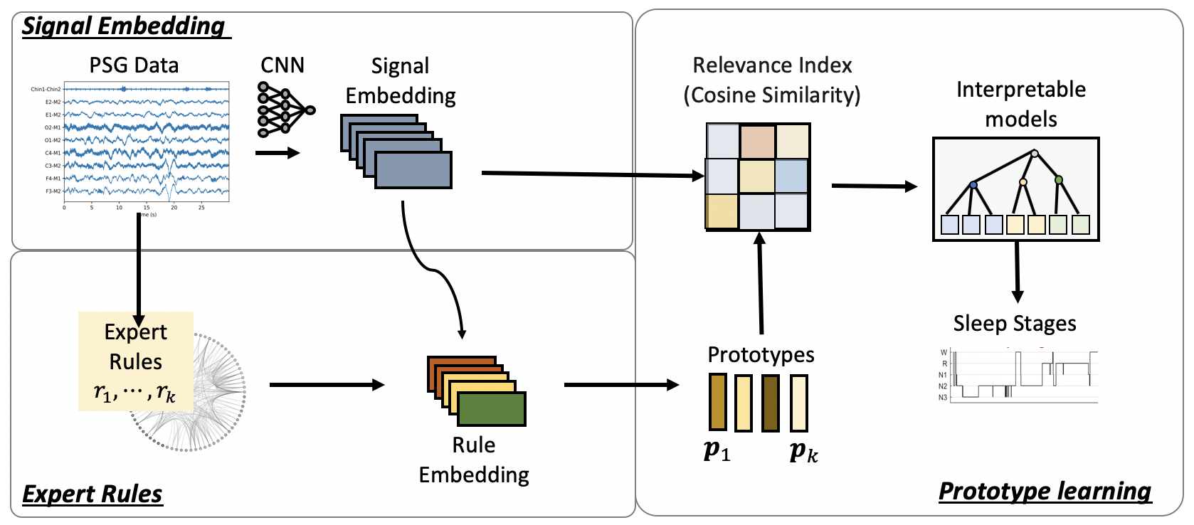
Figure 1: The SLEEPER framework.

2.2 Dataset

To evaluate the performance of SLEEPER, we conducted experiments using two datasets.

MGH This refers to a dataset containing PSG recordings of 2000 subjects from Massachusetts General Hospital. The MGH Institutional Review Board approved retrospective analysis of the clinically acquired data without requiring additional consent. The data was randomly selected from a mixture of diagnostic and split night recordings collected from patients whose ages range from $42$ years old to $64$ years old, with an average age of $53$.

ISRUC This refers to the publicly available ISRUC data (Khalighi et al., 2016). The ISRUC dataset contains PSG recordings of 100 subjects with evidence of having sleep disorders from Sleep Medicine Centre of the Hospital of Coimbra University (CHUC). The data was collected from 55 male and 45 female subjects, whose ages range from $20$ years old to $85$ years old, with an average age of $51$.

The recordings from both dataset were segmented into epochs of 30 seconds and visually scored by sleep technologists according to the guidelines of AASM (Berry et al., 2012). The PSG of both datasets include six EEG channels (F3, F4, C3, C4, O1 and O2), two Electrooculography (EOG) channels (E1 and E2) and a single Electromyography (EMG) channel, each referenced to the contralateral mastoid referred to as M1 and M2, or A1 and A2. Additionally, the ISRUC dataset includes scores by two sleep technologists. We can thus compare the agreement level between two experts and that between an expert and our algorithms.

2.3 Expert Rule Embedding

Majority of the rules in the guideline for sleep technicians (Berry et al., 2012) are vague. For example, LAMF, Low Amplitude Mixed Frequency are shown through multiple visual examples representing samples of the time domain signal but does not specify a threshold for low amplitude or the power distribution across different frequencies. As a result, it is not possible to computationally implement those rules with certainty.

Our approach alleviates the need for discrete boundaries by creating clusters based on the density of the features in each epoch. We incorporate expert suggestion to supplement the technical guidelines in the AASM manual (Berry et al., 2012). Using this rule augmentation procedure, a set of $240$ rules, $\bm{R}^{\prime}=\{r^{\prime}_{1},\;\dots\;r^{\prime}_{240}\}$, are defined. Note that those rules are not directly associated with sleep stage labels like the AASM training manual. Instead, the rules define meaningful phenotypes and the similarity with these phenotypes are used as input features to train sleep stage classifiers later, which lead to robust predictions.

The underlying features in those rules are described below, along with the channels utilized for each feature and the corresponding clustering scheme:

Sleep spindles are bursts of oscillatory signals originating from the thalamus and depicted in EEG (De Gennaro and Ferrara, 2003). It is a discriminatory feature of N2. We used the method proposed by (Lacourse et al., 2019) and (Vallat, 2019) to extract spindles from contralateral signal pairs resulting in: (1) Number of sub-rules: 3 channel pairs with 4 groups for each channel; (2) Channel pairs: i. F3 & F4, ii. C3 & C4, iii. O1 & O2, and (3) Groups: i. $>3$s, ii. $>6$s, iii. $>12$s, iv. $>18$s in an epoch. In total, we have $3\times 4=12$ binary features for spindles. For example, if both F3 and F4 channels exhibit greater than 12 seconds of spindles, the corresponding group will have a feature value 1, and 0 otherwise.

Slow wave sleep (SWS) are distinguished by low-frequency and high-amplitude delta activity. Slow waves are the defining characteristics of N3. We utilize the method proposed by (Carrier et al., 2011), (Massimini et al., 2004), and (Vallat, 2019) to extract SWS from contralateral signal pairs, including (1) Number of sub-rules: 3 channel pairs with 4 groups for each channel, (2) Channel pairs: i. F3 & F4, ii. C3 & C4, iii. O1 & O2, and (3) Groups: i. $>3$s, ii. $>6$s, iii. $>12$s, iv. $>18$s in an epoch.

Delta, Theta, Alpha, and Beta are the frequency bands which play differing roles in sleep staging. Delta (0.5-4Hz) waves delineate N3, Theta (4-8Hz) features in N1, Alpha (8-12Hz) and Beta ($>$12Hz) discriminates between Wake and N1. The four bands in EMG determine the muscle tone used to distinguish between REM and Wake. We find the Power Spectral Density (PSD) using multitaper spectrogram (Gramfort et al., 2014, 2013) in each frequency band and make groups based on the percentile of PSD in the training dataset. (1) Number of sub-rules in each band: 9 channels with 4 groups for each channel, (2) Channels: i. F3, ii. F4, iii. C3, iv. C4, v. O1, vi. O2, vii. E1, viii. E2, ix. Chin EMG, and (3) Groups: i. $<20$th percentile, ii. $<40$th percentile, iii. $<60$th percentile, and iv. $<80$th percentile. In total we have $6\times 4$ binary features for each frequency band. For example, if the PSD of F3 across the Alpha band of an epoch is $<20$ th percentile the corresponding group will have feature value 1, otherwise 0.

Amplitude is important in discriminating Wake, REM, N1 and N2. Features used in sleep staging that are marked by distinctive amplitude include K Complexes, Chin EMG amplitude, Low Amplitude Mixed Frequency (LAMF). Since the AASM manual (Berry et al., 2012) does not declare concrete thresholds, we make groups for each and allow our decision tree to connote significance: (1) Number of sub-rules: 9 channels with 4 groups for each channel, (2) Channels: i. F3, ii. F4, iii. C3, iv. C4, v. O1, vi. O2, vii. E1, viii. E2, ix. Chin EMG, (3) Groups: i. $<20$th percentile, ii. $<40$th percentile, iii. $<60$th percentile, and iv. $<80$th percentile.

Kurtosis denotes the distribution of epochs. Although it is not directly related to any feature used by sleep experts, it helps detect outliers in data such as K Complexes which are rare events marked by a distinctive peak and trough. (1) Number of sub-rules: 9 channels with 4 groups for each channel, (2) Channels: i. F3, ii. F4, iii. C3, iv. C4, v. O1, vi. O2, vii. E1, viii. E2, ix. Chin EMG, (3) Groups: i. $<20$th percentile, ii. $<40$th percentile, iii. $<60$th percentile, and iv. $<80$th percentile.

Phenotype selection

We analyze the efficacy of expert defined rules using ANOVA test and select the most discriminative rules. This reduces the number of expert rules from $240$ to $96$, where $\bm{R}=\{r_{1},\dots r_{96}\}$ and $\bm{R}\subset\bm{R}^{\prime}$. The resulting channels, underlying feature and the number of groups in each feature-channel pair are shown in Table 5. The results from applying all 96 rules on $N$ epochs lead to a binary rule assignment matrix $\bm{R}(\mathcal{X})\in\mathbb{R}^{N\times 96}$, which forms the basis of the interpretation module of SLEEPER framework.

$$\bm{R}(\mathcal{X})=\begin{pmatrix}r_{1}(\bm{X}_{1})&r_{2}(\bm{X}_{1})&\dots\\ r_{1}(\bm{X}_{2})&\ddots&\\ \vdots&&r_{96}(\bm{X}_{N})\end{pmatrix}$$ (1)

where element $r_{j}(\bm{X}_{i})=1\Leftrightarrow$ epoch $\bm{X}_{i}$ satisfies rule $r_{j}$, $\bm{X}_{i}\in\mathcal{X}$, and $\bm{X}_{i}\in\mathbb{R}^{9\times 6,000}$. These resulting features are further discussed in Section 3.3.

2.4 Signal Embedding Generation

The multivariate time series PSG signals were embedded using CNN for capturing translation invariant and complex patterns. The network is composed of 3 convolutional layers as shown in Figure 3. Each convolutional layer is followed by ReLU activation and max pooling. By using a kernel size of 201, the convolutions in the first layer extract features based on 1 second segments of the multivariate time series data.

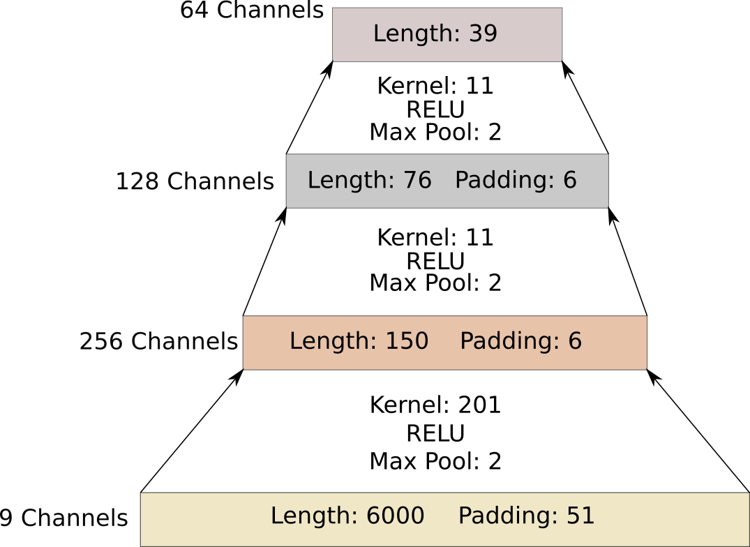
Figure 2: Convolution Layers of CNN

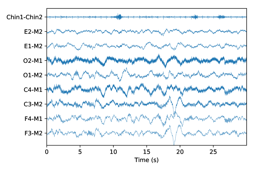
Figure 3: A 30 second epoch having 9 channels

The output of the final convolutional layer, once flattened, is a vector $\bm{h}(\bm{X}_{i})\in\mathbb{R}^{2,496}$. This is followed by a single fully connected layer with softmax activation to predict five different sleep stages:

$$\bm{z}_{i} = \bm{W}^{\top}\bm{h}(\bm{X}_{i})+\bm{b}$$

$$\bm{s}_{i} = \text{softmax}(\bm{z}_{i})$$

where $\bm{W}\in\mathbb{R}^{2,496\times 5}$ is the weight matrix, $\bm{b}\in\mathbb{R}^{5}$ is the bias vector, and $\bm{s}_{i}$ is the estimated probabilities of all 5 sleep stages at epoch $i$. To train the model, we used cross entropy loss in Eq. 2:

$$L(\bm{y}_{i},\;\bm{s}_{i})=-\sum_{j}^{5}\bm{y}_{i}[j]\;log(\bm{s}_{i}[j])$$ (2)

where $L(\bm{y}_{i},\;\bm{s}_{i})$ is the estimated cross entropy loss for epoch $i$ between human labels $\bm{y}\in\mathbb{R}^{5}$ and the predicted probabilities $\bm{s}\in\mathbb{R}^{5}$. After training on sleep stage prediction, we take the latent representation $\bm{h}(\bm{X})$ of 2,496 dimensions as the PSG signal embedding.

2.5 Prototype Learning and Relevance Matching

Each of the 96 rules leads to an embedding representation $\bm{p}_{j}\in\mathbb{R}^{2,496}|j=1,2,\ldots,96$. Next we describe how to construct the embedding of prototypes using the latent representation of all epochs $\bm{h}(\mathcal{X})$. Once we have the rule assignment matrix $\bm{R}(\mathcal{X})$, each prototype representation $\bm{p}_{j}$ corresponds to the sum of latent embeddings of all the epochs that satisfy the rule $j$. Mathematically, all the prototypes can be computed as

$$\bm{P}=\bm{h^{\prime}}(\mathcal{X})^{T}\;\bm{R}(\mathcal{X})$$ (3)

where $\bm{P}\in\mathbb{R}^{2,496\times 96}$ is all the prototype embeddings, $\bm{h^{\prime}}(\mathcal{X})\in\mathbb{R}^{N\times 2,496}$ the column normalized representation of embedded input $\bm{h}(\mathcal{X})$.Next, we use cosine similarity in the embedding space to rank the similarity of any epoch with rules.

$$c_{i,j}=\frac{\bm{h}(\bm{X}_{i})^{\top}\bm{p}_{j}}{||\bm{h}(\bm{X}_{i})||_{2}\;||\bm{p}_{j}||_{2}}$$ (4)

where $c_{i,j}\in[0,1]$ is the cosine similarity between the $i$th epoch and $j$th phenotype and $\bm{C}(\bm{h}(\mathcal{X})|\bm{P})\in\mathbb{R}^{N\times 96}$ .

We use these cosine similarity scores to all prototype embeddings as the input features to simple classifiers. We then train simple and interpretable classifiers such as shallow decision tree and logistic regression to provide the final classifications. When a new PSG, $\bm{X}_{test}$ is given, we find its latent representation using the trained CNN model $\bm{h}(\bm{X}_{test})$, followed by its cosine similarity to existing rule prototypes $\bm{C}(\bm{h}(\bm{X}_{test})|\bm{P})$. Using the simple classifier such as the decision tree, we obtain the predicted sleep stages.

3 Experiments

3.1 Experiment Setting

Baselines. We compare SLEEPER with the following baseline models on both datasets:

• Convolutional Neural Network (CNN) is the blackbox model used in obtaining the signal embeddings. It serves as the performance upper bound;

• Rules with Interpretable Classifier where each epoch is represented by a multi-hot encoded binary rule assignment vector $\bm{R}(\bm{X_{i}})$ from eqn. 1 and classification using gradient boosting (GB), decision tree (DT), and logistic regression (LR), respectively. For the choice of interpretable model in SLEEPER, we also consider DT, LR and GB.

• Mimic learning (Che et al., 2015) where the soft labels from RCNN are used instead of the original hard labels and a gradient boosting regressor is then trained with those soft labels.

Additionally, on ISRUC dataset we also compare with the following baselines across 5 different sleep stages: (1) Agreement between two sleep experts on the same PSG recordings; (2) Maximum Overlap Discrete Wavelet Transform (MODWT) (Khalighi et al., 2016, 2013); (3) Logistic Smooth Transition Autoregressive (LSTAR) (Ghasemzadeh et al., 2019) (4) Convolutional Neural Network (CNN) (Chambon et al., 2018) (5) RCNN on Spectrogram (Biswal et al., 2018). Note that (1) and (2) are conducted on the same ISRUC dataset, while (3-5) are on different datasets, which are only for rough comparison.

Metrics. We compared testing performance using the following metrics, including accuracy ($Acc$), area under the receiver operator characteristics curve (ROC-AUC), and Cohen’s $\kappa$. Here, Cohen’s $\kappa$ considers the possibility of assigning the correct sleep stage through random guesses. According to (Viera et al., 2005), $\kappa>0.81,\;0.8>\kappa>0.61,\;0.6>\kappa>0.41,\;0.4>\kappa>0.21,\;0.2>\kappa>0.01,\;\kappa<0.01$, means almost perfect, substantial, moderate, fair, slight, less than chance agreement respectively. We compare the performance across the 5 sleep stages using confusion matrices and class-wise sensitivity ($Sens^{(k)}$), also known as recall. Given expert annotations, $\mathcal{Y}^{\prime}$ and predicted stages, $\mathcal{Y}$ of size $N$, $k=\{1,2,3,4,5\}$ indicating the sleep stage,

$$Acc=\frac{|\mathcal{Y}\cap\mathcal{Y}^{\prime}|}{N},\quad Sens^{(k)}=\frac{\left|\mathcal{Y}^{(k)}\cap\mathcal{Y}^{\prime(k)}\right|}{\left|\mathcal{Y}^{\prime(k)}\right|}\;$$

$$\kappa=\frac{Acc-p_{e}}{1-p_{e}},\text{ where }p_{e}=\frac{1}{N^{2}}\sum_{k}^{5}\left|\mathcal{Y}^{(k)}\right|\left|\mathcal{Y}^{\prime(k)}\right|$$

and $|\mathcal{Y^{\prime}}^{(k)}|$ ($|\mathcal{Y}^{(k)}|$)is the number of human (algorithm) labels from sleep stage $k$.

Implementation Details. We implemented SLEEPER in PyTorch 1.0 (Paszke et al., 2017) and scikit-learn (Pedregosa et al., 2011). We train the model using a machine equipped with Intel Xeon e5-2640, 256GB RAM, eight Nvidia Titan-X GPU and CUDA 10.0. While training the CNN, we use batch size of 1 PSG and ADAM as the optimization method. We train the CNN for 40 epochs. We set the learning rate at $10^{-4}$ and divide the learning rate by 10 once after 10 epochs.

To train the model, we randomly split the data by subjects into training and testing in a 9:1 ratio. For each dataset, we train using the training set to fix model parameters and test on the testing set for performance comparison. To ensure consistent performance across different datasets, we use the same model hyperparameters and underlying feature extraction schema to test both datasets. To evaluate SLEEPER, we consider the following baselines and evaluation metrics.

3.2 Results on Staging Accuracy

The experimental results are compared in Table 2. On both datasets, SLEEPER performs almost as accurately as the black-box neural network models. Although SLEEPER achieved significant reduction in dimensionality, from $\mathbb{R}^{2,496}$ to $\mathbb{R}^{96}$, the difference in AUC-ROC, accuracy, and Cohen’s $\kappa$ to the black-box CNN is relatively small. Moreover, each of those $96$ dimensions are interpretable. SLEEPER-Decision Tree provides a list of normalized indices of length equal to the depth of the tree to indicate similarity with meaningful rules.

Model	Accuracy $(\%)$		ROC-AUC $(\%)$		Cohen’s $\kappa$
	MGH	ISRUC	MGH	ISRUC	MGH	ISRUC
SLEEPER-DT	78.3	78.5	85.0	84.7	0.694	0.720
SLEEPER-LR	79.8	77.0	86.1	84.9	0.714	0.699
SLEEPER-GBT	78.8	80.1	85.4	86.0	0.700	0.741
Rule & DT	66.1	67.1	75.7	78.2	0.510	0.564
Rule & LR	65.3	69.1	75.0	79.0	0.498	0.593
Rule & GBT	65.8	69.3	75.3	78.8	0.508	0.594
Mimic learning - GBT	67.5	62.1	78.6	76.4	0.540	0.514
CNN	81.6	82.4	87.4	87.8	0.742	0.772

Table 1: Model Evaluation. DT: Decision Tree, LR: Logistic Regression, GBT: Gradient Boosting Trees, Rule: Binary Features from Rules, CNN: Convolutional Neural Network

Model	Sensitivity $(\%)$
	Wake	REM	N1	N2	N3
SLEEPER-DT	88.3	85.3	26.9	82.59	85.6
SLEEPER-LR	87.9	80.6	27.3	84.4	79.1
SLEEPER-GBT	88.1	86.1	34.5	83.2	87.9
Human Expert Agreement	92.4	91.2	55.4	86.6	77.4
MODWT (Khalighi et al., 2016)	88.3	81.8	39.3	80.2	83.5
CNN (Chambon et al., 2018)	85	83	52	77	91
LSTAR (Ghasemzadeh et al., 2019)	88.7	88.4	50.3	85.0	87.4
RCNN on Spectrogram (Biswal et al., 2018)	85	92	58	89	86

Table 2: Sensitivity across Sleep Stages . DT: Decision Tree, GB: Gradient Boosting Trees, LR: Logistic Regression,

The sensitivity in classifying each sleep stage is compared with baselines in Table 4. The confusion matrices of our results using ISRUC dataset is shown in Figure LABEL:fig:conf_mat. Agreement between experts are shown in Figure LABEL:fig:inter_rater and SLEEPER using a decision tree in Figure LABEL:fig:conf_prototype. N1 classification is particularly problematic even for human sleep experts. This is due to significant overlap in underlying criteria with N2. Beyond N2, SLEEPER with Decision Tree surpass the performance of the baseline automatic sleep staging algorithm (Khalighi et al., 2013) while also providing interpretation. It exceeds expert agreement by a significant margin for N3. Reasons for this are further discussed in Section 3.4.

The agreement between two human experts in assigning sleep stages to our test PSGs in the ISRUC dataset is 83.0%, with a Cohen $\kappa$ of 0.78. SLEEPER using a decision tree obtains an accuracy of 78.5%, with a Cohen’s $\kappa$ of 0.72 indicating substantial agreement according to the guidelines from (Viera et al., 2005).

Figure LABEL:fig:tree_deep shows the change in ROC-AUC of SLEEPER and rule based method with depth of tree. It shows for trees of depth 9 we obtain ROC-AUC greater than 84% in both ISRUC and MGH Datasets. This indicates, a group of 9 meaningful prototypes is able to classify the sleep stage in a sample well. Note, the larger size of MGH Dataset results in a much smoother distribution but the overall performance remain similar. This shows robustness across different datasets and the significant performance improvement from rules using SLEEPER.

3.3 Feature Selection Results of Expert Rules

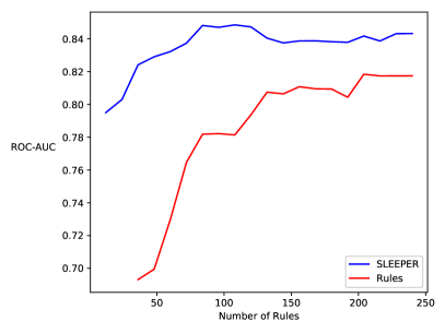
Figure 8: SLEEPER ROC-AUC vs Number of Rules

Channels	Features
	Spindle	SWS	Delta	Theta	Alpha	Beta	Kurtosis	Amplitude
F3-A2		3	4		4	4		4
F4-A1		3	4	4	4			4
C3-A2		2	4	4		4		4
C4-A1		2	4					4
O1-A2			4	4				4
O2-A1			4	3	4			4
ROC-A2			4					4
LOC-A2
Chin EMG

Table 3: 96 selected rules out of 240 expert rules using ISRUC dataset

Instead of handpicking due to ambiguity in their significance, we use analysis of variance (ANOVA) models to rank features by significance and reduce the number of rules from 240 to 96. The change in ROC-AUC with number of rules is shown in Figure 8. It reveals the discrepancy in performance between SLEEPER and the rule based method. The selected number of expert rules from each channel-feature pair is shown in Table 5. Note that the selected features do not include any features from Spindles and Kurtosis. In particular, sleep spindles have frequency range of 12-14 Hz with a duration of 0.5-1.5 seconds but their use in detecting N2 is practically difficult. This could be due to hidden spindles in other stages (Lacourse et al., 2019). And Kurtosis is a common statistical measure but is not directly related to key features described in sleep scoring manual. We also observe the removal of rules using EMG and second EOG channels. EMG recordings are particularly noisy with low amplitude, as shown in the top channel of Figure 3.

K Complex, another underlying feature in N2 and REM detection, contains a distinctive rise and fall which is larger than the amplitude of regular signal oscillations. K Complexes, unfortunately, are not relibable enough for our use case with an inter-rater $\kappa$ of .51 (Lajnef et al., 2015). On the other hand, amplitude based prototypes play a big role in SLEEPER. Low Amplitude Mixed Frequency (LAMF) is a feature used for discriminating Wake, N1, N2 and REM. The channels used in detecting LAMF are not mentioned in the guidelines (Berry et al., 2012).

3.4 Interpretation

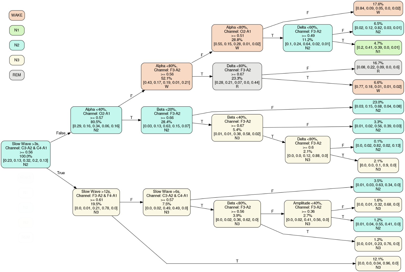
Figure 9: SLEEPER-Decision Tree trained from the ISRUC dataset

Figure 9 shows a decision tree of depth, $D=5$, based on SLEEPER. This obtains an AUC-ROC of 81%. The leftmost node denotes the root of the tree and the colour indicates the most frequent sleep stage for training data passing through that node. The six rows of each node contains the following: (1) the underlying feature and grouping criteria, (2) the channels used to extract the feature, (3) the cosine similarity with the resulting rule, (4) the percentage of data passing through the node, (5) the ratio of the each sleep stage in data passing through the node in the following order: [Wake, N1, N2, N3, REM], (6) the most frequent sleep stage at the node, in other words, if classification is performed at that node we will assign this label. The leaves on the right contain the same contents as lowest 3 rows at other nodes.

Analyzing the resulting decision tree reveals some promising aspects of SLEEPER. According to the sleep staging guidelines for human annotators (Berry et al., 2012), N3 is distinguished by occurrence of slow waves. One of the underlying features of our rules is slow waves. We created 4 binary features based on the duration of slow wave in each 30s epoch, $>3$s, $>6$s, $>12$s, and $>18$s. The first node creates a split based on cosine similarity $\geq 0.56$ with the prototype, Slow Waves of duration greater than 3s in the Central Channels. Since slow waves are predominant in N3, $78\%$ of training data that satisfied the aforementioned criteria in the next node contains N3, while only $6\%$ of the other child contains N3. The next node restricts the threshold to 12s in the Frontal region. $96\%$ of the resulting leaf node classifying $12.1\%$ of the training dataset was labelled, in agreement with SLEEPER, as N3 by experts.

Furthermore, analyzing the leaves, we observe stages with similar characteristics occur in pairs, like REM and Wake, N3 and N2, N1 and N2. We notice that top right leaf containing Wake is distinguished by Alpha activity in the Occipital Region. This criteria for detecting Wake is mentioned in the guidelines for human annotators (Berry et al., 2012).

4 Conclusion

Interpretability and accuracy are often trade-off to each other in machine learning modeling. Especially in the age of deep learning, many accurate models are black-box models that do not provide any insights into the reasoning behind predictions. On the other hand, simple models like decision trees often result in inaccurate predictors. In this paper, we present SLEEPER that introduces a deep prototype learning method that provides accurate predictions as well as very simple and intuitive prediction models with a shallow decision tree. We develop and evaluate the methods in the context of sleep staging applications on PSG data from sleep labs. SLEEPER achieves high accuracy in sleep staging tasks comparable to state of the art baselines. A qualitative case study illustrated a simple and intuitive decision tree that can perform accurate sleep staging classification while providing explanation through interpretable rules.

Appendix A. Feature Selected from MGH Dataset

Channels	Features
	Spindle	SWS	Delta	Theta	Alpha	Beta	Kurtosis	Amplitude
F3-M2		3	4	4	4	4		4
F4-M1		3	4	4	4			4
C3-M2		3	4	4				4
C4-M1		3	4					4
O1-M2		2	4	4				4
O2-M1		2	4	4				4
E1-M2					4			4
E2-M2
Chin1-Chin2

Table 4: 96 selected rules out of 240 expert rules using MGH Dataset

References

- ASA (2019) ASA. Sleep statistics - research & treatments — american sleep assoc. https://www.sleepassociation.org/about-sleep/sleep-statistics/, 2019.
- Berry et al. (2012) Richard B Berry, Rohit Budhiraja, Daniel J Gottlieb, David Gozal, Conrad Iber, Vishesh K Kapur, Carole L Marcus, Reena Mehra, Sairam Parthasarathy, Stuart F Quan, et al. Rules for scoring respiratory events in sleep: update of the 2007 aasm manual for the scoring of sleep and associated events. Journal of clinical sleep medicine, 8(05):597–619, 2012.
- Bien and Tibshirani (2011) Jacob Bien and Robert Tibshirani. Prototype selection for interpretable classification. The Annals of Applied Statistics, pages 2403–2424, 2011.
- Biswal et al. (2018) Siddharth Biswal, Jimeng Sun, Haoqi Sun, M Brandon Westover, Balaji Goparaju, and Matt T Bianchi. Expert-level sleep scoring with deep neural networks. Journal of the American Medical Informatics Association, 25(12):1643–1650, 11 2018. ISSN 1527-974X. 10.1093/jamia/ocy131. URL https://doi.org/10.1093/jamia/ocy131.
- Carrier et al. (2011) Julie Carrier, Isabelle Viens, Gaétan Poirier, Rébecca Robillard, Marjolaine Lafortune, Gilles Vandewalle, Nicolas Martin, Marc Barakat, Jean Paquet, and Daniel Filipini. Sleep slow wave changes during the middle years of life. European Journal of Neuroscience, 33(4):758–766, 2011.
- Chambon et al. (2018) Stanislas Chambon, Mathieu N Galtier, Pierrick J Arnal, Gilles Wainrib, and Alexandre Gramfort. A deep learning architecture for temporal sleep stage classification using multivariate and multimodal time series. IEEE Transactions on Neural Systems and Rehabilitation Engineering, 26(4):758–769, 2018.
- Che et al. (2015) Zhengping Che, Sanjay Purushotham, Robinder Khemani, and Yan Liu. Distilling knowledge from deep networks with applications to healthcare domain. arXiv preprint arXiv:1512.03542, 2015.
- De Gennaro and Ferrara (2003) Luigi De Gennaro and Michele Ferrara. Sleep spindles: an overview. Sleep medicine reviews, 7(5):423–440, 2003.
- Dong et al. (2018) Hao Dong, Akara Supratak, Wei Pan, Chao Wu, Paul M Matthews, and Yike Guo. Mixed neural network approach for temporal sleep stage classification. IEEE Transactions on Neural Systems and Rehabilitation Engineering, 26(2):324–333, 2018.
- Doshi-Velez and Kim (2017) Finale Doshi-Velez and Been Kim. Towards a rigorous science of interpretable machine learning. arXiv preprint arXiv:1702.08608, 2017.
- Ghasemzadeh et al. (2019) Peyman Ghasemzadeh, Hashem Kalbkhani, Shadi Sartipi, and Mahrokh G Shayesteh. Classification of sleep stages based on lstar model. Applied Soft Computing, 75:523–536, 2019.
- Gramfort et al. (2013) Alexandre Gramfort, Martin Luessi, Eric Larson, Denis A Engemann, Daniel Strohmeier, Christian Brodbeck, Roman Goj, Mainak Jas, Teon Brooks, Lauri Parkkonen, et al. Meg and eeg data analysis with mne-python. Frontiers in neuroscience, 7:267, 2013.
- Gramfort et al. (2014) Alexandre Gramfort, Martin Luessi, Eric Larson, Denis A Engemann, Daniel Strohmeier, Christian Brodbeck, Lauri Parkkonen, and Matti S Hämäläinen. Mne software for processing meg and eeg data. Neuroimage, 86:446–460, 2014.
- Khalighi et al. (2013) Sirvan Khalighi, Teresa Sousa, Gabriel Pires, and Urbano Nunes. Automatic sleep staging: A computer assisted approach for optimal combination of features and polysomnographic channels. Expert Systems with Applications, 40(17):7046–7059, 2013.
- Khalighi et al. (2016) Sirvan Khalighi, Teresa Sousa, José Moutinho Santos, and Urbano Nunes. Isruc-sleep: a comprehensive public dataset for sleep researchers. Computer methods and programs in biomedicine, 124:180–192, 2016.
- Kim et al. (2014) Been Kim, Cynthia Rudin, and Julie A Shah. The bayesian case model: A generative approach for case-based reasoning and prototype classification. In Advances in Neural Information Processing Systems, pages 1952–1960, 2014.
- Kolodner (1992) Janet L Kolodner. An introduction to case-based reasoning. Artificial intelligence review, 6(1):3–34, 1992.
- Krieger (2017) Ana C Krieger. Social and Economic Dimensions of Sleep Disorders, An Issue of Sleep Medicine Clinics, E-Book, volume 12. Elsevier Health Sciences, 2017.
- Lacourse et al. (2019) Karine Lacourse, Jacques Delfrate, Julien Beaudry, Paul Peppard, and Simon C Warby. A sleep spindle detection algorithm that emulates human expert spindle scoring. Journal of neuroscience methods, 316:3–11, 2019.
- Lajnef et al. (2015) Tarek Lajnef, Sahbi Chaibi, Jean-Baptiste Eichenlaub, Perrine Marie Ruby, Pierre-Emmanuel Aguera, Mounir Samet, Abdennaceur Kachouri, and Karim Jerbi. Sleep spindle and k-complex detection using tunable q-factor wavelet transform and morphological component analysis. Frontiers in human neuroscience, 9:414, 2015.
- Längkvist et al. (2012) Martin Längkvist, Lars Karlsson, and Amy Loutfi. Sleep stage classification using unsupervised feature learning. Adv. Artif. Neu. Sys., 2012:5:5–5:5, January 2012. ISSN 1687-7594. 10.1155/2012/107046. URL http://dx.doi.org/10.1155/2012/107046.
- Li et al. (2017) Oscar Li, Hao Liu, Chaofan Chen, and Cynthia Rudin. Deep learning for case-based reasoning through prototypes: A neural network that explains its predictions. CoRR, abs/1710.04806, 2017. URL http://arxiv.org/abs/1710.04806.
- Lipton (2016) Zachary Chase Lipton. The mythos of model interpretability. CoRR, abs/1606.03490, 2016. URL http://arxiv.org/abs/1606.03490.
- Massimini et al. (2004) Marcello Massimini, Reto Huber, Fabio Ferrarelli, Sean Hill, and Giulio Tononi. The sleep slow oscillation as a traveling wave. Journal of Neuroscience, 24(31):6862–6870, 2004.
- Paszke et al. (2017) Adam Paszke, Sam Gross, Soumith Chintala, Gregory Chanan, Edward Yang, Zachary DeVito, Zeming Lin, Alban Desmaison, Luca Antiga, and Adam Lerer. Automatic differentiation in pytorch. In NIPS-W, 2017.
- Pedregosa et al. (2011) F. Pedregosa, G. Varoquaux, A. Gramfort, V. Michel, B. Thirion, O. Grisel, M. Blondel, P. Prettenhofer, R. Weiss, V. Dubourg, J. Vanderplas, A. Passos, D. Cournapeau, M. Brucher, M. Perrot, and E. Duchesnay. Scikit-learn: Machine learning in Python. Journal of Machine Learning Research, 12:2825–2830, 2011.
- Priebe et al. (2003) Carey E Priebe, David J Marchette, Jason G DeVinney, and Diego A Socolinsky. Classification using class cover catch digraphs. Journal of classification, 20(1):003–023, 2003.
- Schutte-Rodin et al. (2008) Sharon Schutte-Rodin, Lauren Broch, Daniel Buysse, Cynthia Dorsey, and Michael Sateia. Clinical guideline for the evaluation and management of chronic insomnia in adults. Journal of Clinical Sleep Medicine, 4(05):487–504, 2008.
- Snell et al. (2017) Jake Snell, Kevin Swersky, and Richard S. Zemel. Prototypical networks for few-shot learning. CoRR, abs/1703.05175, 2017. URL http://arxiv.org/abs/1703.05175.
- Sors et al. (2018) Arnaud Sors, Stéphane Bonnet, Sébastien Mirek, Laurent Vercueil, and Jean-François Payen. A convolutional neural network for sleep stage scoring from raw single-channel eeg. Biomedical Signal Processing and Control, 42:107–114, 2018.
- Stephansen et al. (2018) Jens B Stephansen, Alexander N Olesen, Mads Olsen, Aditya Ambati, Eileen B Leary, Hyatt E Moore, Oscar Carrillo, Ling Lin, Fang Han, Han Yan, et al. Neural network analysis of sleep stages enables efficient diagnosis of narcolepsy. Nature communications, 9(1):5229, 2018.
- Vallat (2019) Raphael Vallat. raphaelvallat/yasa: v0.1.3, March 2019. URL https://doi.org/10.5281/zenodo.2583431.
- Viera et al. (2005) Anthony J Viera, Joanne M Garrett, et al. Understanding interobserver agreement: the kappa statistic. Fam med, 37(5):360–363, 2005.