Symplectic model reduction methods for the Vlasov equation

Abstract

Particle-based simulations of the Vlasov equation typically require a large number of particles, which leads to a high-dimensional system of ordinary differential equations. Solving such systems is computationally very expensive, especially when simulations for many different values of input parameters are desired. In this work we compare several model reduction techniques and demonstrate their applicability to numerical simulations of the Vlasov equation. The necessity of symplectic model reduction algorithms is illustrated with a simple numerical experiment.

1 Introduction

Kinetic models like the Vlasov equation provide the most accurate description for a plasma beyond the interaction of individual particles. While physically comprehensive, such models are often too expensive to be solved numerically under realistic conditions, especially in many-query contexts like uncertainty quantification, inverse problems or optimization. In such situations reduced complexity models can provide a good compromise between computational cost and physical completeness of numerical models, and facilitate the solution of problems that are otherwise unfeasible.

A common approach for the construction of reduced complexity models are modal decomposition techniques such as proper orthogonal decomposition (POD, see [5]), also known as principal component analysis (PCA, see [34]), and dynamic mode decomposition (DMD, see [4]). Here, existing complex models are replaced by reduced models, which preserve the essential features of the original systems, but require less computational effort.

Algorithms obtained by such model order reduction techniques usually consist of two stages: an offline stage, where the reduced basis is constructed from empirical or simulation data of a physical system, referred to as snapshots, and an online stage, where the system is solved in the reduced basis. These techniques use singular-value decomposition (SVD) to identify dominant global modes in the snapshots, in such a way that the basis constructed from these modes spans the data optimally. Standard Galerkin projection methods are used to obtain approximate operators on such a basis (see [26]). This approach is often amended by techniques such as the discrete empirical interpolation method to allow for efficient evaluation of nonlinearities (see [12]).

While model order reduction has been successfully applied to finite difference and finite volume discretizations of fluid equations (see [28] for an overview), its applicability is not yet well studied for kinetic equations. Thus the main goal of this work is to demonstrate the usefulness of model reduction techniques for numerical simulations of the Vlasov equation using particle methods. Further, we will show that preserving the Hamiltonian structure of the system in the reduction procedure is key to obtaining stable and accurate reduced models.

1.1 Particle methods for the Vlasov equation

In this work we consider the Vlasov equation

$$\frac{\partial f}{\partial t}+v\frac{\partial f}{\partial x}-E(x)\frac{\partial f}{\partial v}=0,$$ (1.1)

for the particle density function $f=f(t,x,v)$ of plasma consisting of charged particles of unit mass and unit negative charge, where $E(x)=-\frac{\partial\phi}{\partial x}$ is an external electrostatic field with the potential $\phi=\phi(x)$, and $x$ and $v$ are vectors in $\mathbb{R}^{d}$ with $d=1,2,3$. The standard approach to particle methods consists of the Ansatz

$$f(t,x,v)=\sum_{i=1}^{n}w_{i}\delta(x-X_{i}(t))\delta(v-V_{i}(t))$$ (1.2)

for the particle density function, where $X_{i}(t)$ and $V_{i}(t)$ represent the position and velocity of the $i$-th particle, respectively, and $w_{i}$ its weight. Substituting (1.2) in (1.1), one obtains a system of ordinary differential equations (ODEs) for $X_{i}(t)$ and $V_{i}(t)$, namely

$$\dot{X}_{i} =V_{i},$$

$$\dot{V}_{i} =\frac{\partial\phi}{\partial x}(X_{i}),\qquad\qquad i=1,\ldots,n.$$ (1.3)

It can be easily verified that (1.1) has the form of a Hamiltonian system of equations

$$\dot{X}_{i} =\frac{\partial H}{\partial V_{i}},$$

$$\dot{V}_{i} =-\frac{\partial H}{\partial X_{i}},\qquad\qquad i=1,\ldots,n,$$ (1.4)

with the Hamiltonian $H$ given by

$$H(X,V)=\sum_{i=1}^{n}\Big{[}\frac{1}{2}V_{i}^{2}-\phi(X_{i})\Big{]},$$ (1.5)

where $X=(X_{1},\ldots,X_{n})$ and $V=(V_{1},\ldots,V_{n})$ are vectors in $\mathbb{R}^{nd}$. Note that, for simplicity and brevity, we express the Hamiltonian in terms of the velocity vector $V$ rather than the canonical conjugate momentum vector $P$, since for a fixed external electric field and particles of unit mass we have $P_{i}=V_{i}$.

1.2 Geometric integration

The Hamiltonian system (1.1) possesses several characteristic properties. Its flow $F_{t}:\mathbb{R}^{2nd}\longrightarrow\mathbb{R}^{2nd}$ preserves the Hamiltonian, i.e. the total energy, as well as the canonical symplectic form $\omega=\sum_{i=1}^{n}\sum_{j=1}^{d}dX_{i}^{j}\wedge dV_{i}^{j}$. The latter property expressed in terms of the standard basis for $\mathbb{R}^{2nd}$ takes the form of the condition

$$(DF_{t})^{T}\mathbb{J}_{2nd}DF_{t}=\mathbb{J}_{2nd},$$ (1.6)

where $DF_{t}$ denotes the Jacobi matrix of the flow map $F_{t}$, $\mathbb{J}_{2nd}$ denotes the canonical symplectic matrix defined as

$$\mathbb{J}_{2nd}=\left(\begin{matrix}0&\mathbb{I}_{nd}\\ -\mathbb{I}_{nd}&0\end{matrix}\right),$$ (1.7)

and $\mathbb{I}_{nd}$ is the $nd\times nd$ identity matrix (see, e.g., [14], [19], [30]).

In principle, general purpose numerical schemes for ODEs can be applied to Hamiltonian systems such as (1.1). However, when simulating these systems numerically, it is advisable that the numerical scheme also preserves geometric features such as symplecticity (1.6). Geometric integration of Hamiltonian systems has been thoroughly studied (see [14], [16], [21], [22], [29], [31], [32], [33], [35], [46], [47], [48], [51], [52] and the references therein) and symplectic integrators have been shown to demonstrate superior performance in long-time simulations of such systems, compared to non-symplectic methods. Long-time accuracy and near preservation of the Hamiltonian by symplectic integrators have been rigorously studied using the so-called backward error analysis (see, e.g., [14] and the references therein). Application of geometric integration to particle-in-cell (PIC) simulations of the Vlasov equation coupled to self-consistent electromagnetic fields satisfying the Maxwell equations (i.e., the Vlasov-Maxwell system) was proposed in [23], [44], [53], [54], [55].

1.3 Symplectic model reduction

For the aforementioned reasons it appears desirable to preserve the Hamiltonian structure also in model reduction. In fact, it has been found that preserving the Hamiltonian structure in the construction of the reduced spaces preserves stability [1], which is not guaranteed using non-structure-preserving model reduction techniques ([43], [45]). To this end, standard model reduction techniques such as proper orthogonal decomposition have been modified towards the so-called proper symplectic decomposition ([39], [40], [41]), which does indeed preserve the canonical symplectic structure of many Hamiltonian systems in the reduction procedure. Similarly, greedy algorithms ([1], [2], [3]) can be used to construct the reduced basis in a Hamiltonian-structure preserving way, and recently also non-orthonormal bases have been considered [6], showing improved efficiency over orthonormal bases. See also [9], [11], [17], [27].

1.4 Outline

The main content of the remainder of this paper is, as follows. In Section 2 we review several model reduction techniques and set the appropriate notation. In Section 3 we present the results of our numerical experiment demonstrating the applicability of model reduction techniques to particle methods for the Vlasov equation. Section 4 contains the summary of our work.

2 Model reduction

In this section we briefly review several model reduction techniques and set the notation appropriate for the problem defined in the introduction.

2.1 Proper orthogonal decomposition

Proper orthogonal decomposition (POD) is one of the standard model reduction techniques (see [5], [34]). Consider a general ODE

$$\dot{u}=g(u),\qquad\qquad\text{with $g:\mathbb{R}^{N}\longrightarrow\mathbb{R}^{N}$},$$ (2.1)

and with the initial condition $u(0)=u_{0}$. Equation (1.1) has this form with $N=2nd$, $u=(X,V)$, and $g(u)=(V_{1},\ldots,V_{n},\frac{\partial\phi}{\partial x}(X_{1}),\ldots,\frac{\partial\phi}{\partial x}(X_{n}))$. When $N$ is a very high number, as is typical for particle methods, the system (2.1) becomes very expensive to solve numerically. The main idea of model reduction is to approximate such a high-dimensional dynamical system using a lower-dimensional one that can capture the dominant dynamic properties. Let $\Delta$ be an $N\times M$ matrix representing empirical data on the system (2.1). For instance, $\Delta$ can be a collection of snapshots of a solution of this system,

$$\Delta=[u(t_{1})\,\,u(t_{2})\,\,\ldots\,\,u(t_{M})],$$ (2.2)

at times $t_{1},\ldots,t_{M}$. These snapshots are calculated for some particular initial conditions or values of parameters that the system (2.1) depends on. A low-rank approximation of $\Delta$ can be done by performing a singular value decomposition (SVD) of $\Delta$ and truncating it after the first $K$ largest singular values, that is,

$$\Delta=U\Sigma V^{T}\approx U_{K}\Sigma_{K}V_{K}^{T},$$ (2.3)

where $\Sigma=\text{diag}(\sigma_{1},\sigma_{2},\ldots)$ is the diagonal matrix of the singular values, $U$ and $V$ are orthogonal matrices, $\Sigma_{K}$ is the diagonal matrix of the first $K$ largest singular values, and $U_{K}$ and $V_{K}$ are orthogonal matrices constructed by taking the first $K$ columns of $U$ and $V$, respectively. Let $\xi$ denote a vector in $\mathbb{R}^{K}$. Substituting $u=U_{K}\xi$ in (2.1) yields a reduced ODE for $\xi(t)$ as

$$\dot{\xi}=U_{K}^{T}g(U_{K}\xi),$$ (2.4)

with the projected initial condition $\xi(0)=\xi_{0}=U_{K}^{T}u_{0}$. If the singular values of $\Delta$ decay sufficiently fast, then one can obtain a good approximation of $\Delta$ for $K$ such that $K\ll N$ (see Section 2.3). Equation (2.4) is then a low-dimensional approximation of (2.1) and can be solved more efficiently. For more details about the POD method we refer the reader to [5]. In the context of particle methods for the Vlasov equation, the reduced model (2.4) allows one to perform numerical computations with a much smaller number of degrees of freedom. Note, however, that while (1.1) is a Hamiltonian system, there is no guarantee that the reduced model (2.4) will also have that property. In Section 3 we demonstrate that retaining the Hamiltonian structure in the reduced model greatly improves the quality of the numerical solution.

2.2 Proper symplectic decomposition

Note that the Hamiltonian system (1.1) can be equivalently written as

$$\dot{u}=\mathbb{J}_{2N}\nabla_{u}H(u),$$ (2.5)

where $u=(X,V)$ and $N=nd$. A model reduction technique that retains the symplectic structure of Hamiltonian systems was introduced in [41]. In analogy to POD, this method is called the proper symplectic decomposition (PSD). A $2N\times 2K$ matrix is called symplectic if it satisfies the condition

$$A^{T}\mathbb{J}_{2N}A=\mathbb{J}_{2K}.$$ (2.6)

For a symplectic matrix $A$, we can define its symplectic inverse $A^{+}=\mathbb{J}_{2K}^{T}A^{T}\mathbb{J}_{2N}$. It is an inverse in the sense that $A^{+}A=\mathbb{I}_{2K}$. Let $\xi$ be a vector in $\mathbb{R}^{2K}$. Substituting $u=A\xi$ in (2.5) yields a reduced equation

$$\dot{\xi}=A^{+}\mathbb{J}_{2N}\nabla_{u}H(u)=\mathbb{J}_{2K}\nabla_{\xi}H(A\xi),$$ (2.7)

which is a lower-dimensional Hamiltonian system with the Hamiltonian $\tilde{H}(\xi)=H(A\xi)$. Given a set of empirical data on a Hamiltonian system, the PSD method constructs a symplectic matrix $A$ which best approximates that data in a lower-dimensional subspace. We have tested two PSD algorithms, namely the cotangent lift and complex SVD algorithms.

2.2.1 Cotangent lift algorithm

This algorithm constructs a symplectic matrix $A$ which has the special block diagonal structure

$$A=\left(\begin{matrix}\Phi&0\\ 0&\Phi\end{matrix}\right),$$ (2.8)

where $\Phi$ is an $N\times K$ matrix with orthogonal columns, i.e. $\Phi^{T}\Phi=\mathbb{I}_{K}$. Suppose snapshots of a solution are given as an $N\times 2M$ matrix $\Delta$ of the form

$$\Delta=[X(t_{1})\,\,\ldots\,\,X(t_{M})\,\,V(t_{1})\,\,\ldots\,\,V(t_{M})].$$ (2.9)

The SVD of $\Delta$ is truncated after the first $K$ largest singular values, similar to (2.3). The matrix $\Phi$ is then chosen as $\Phi=U_{K}$. More details can be found in [41].

2.2.2 Complex SVD algorithm

By allowing a broader class of symplectic matrices we may get a better approximation. The complex SVD algorithm constructs a symplectic matrix of the form

$$A=\left(\begin{matrix}\Phi&-\Psi\\ \Psi&\Phi\end{matrix}\right),$$ (2.10)

where $\Phi$ and $\Psi$ are $N\times K$ matrices satisfying the conditions

$$\Phi^{T}\Phi+\Psi^{T}\Psi=\mathbb{I}_{K},\qquad\qquad\Phi^{T}\Psi=\Psi^{T}\Phi.$$ (2.11)

Suppose snapshots of a solution are given as an $N\times M$ complex matrix $\Delta$ of the form

$$\Delta=[X(t_{1})+iV(t_{1})\,\,\ldots\,\,X(t_{M})+iV(t_{M})],$$ (2.12)

where $i$ denotes the imaginary unit. The complex SVD of $\Delta$ is truncated after the first $K$ largest singular values, that is,

$$\Delta=U\Sigma V^{\dagger}\approx U_{K}\Sigma_{K}V_{K}^{\dagger}.$$ (2.13)

The matrices $\Phi$ and $\Psi$ are then chosen as the real and imaginary parts of $U_{K}$, respectively, that is, $U_{K}=\Phi+i\Psi$. More details can be found in [41].

2.2.3 Preservation of the Hamiltonian

Let $u(t)$ be a solution of (2.5) with the initial condition $u_{0}$, and let $\xi(t)$ be a solution of the reduced system (2.7) with the projected initial condition $\xi_{0}=A^{+}u_{0}$. Since the solutions of both the unreduced and reduced equations preserve their respective Hamiltonians, we have that the error of the Hamiltonian $\Delta H(t)=H(u(t))-\tilde{H}(\xi(t))$ arising due to the symplectic projection is constant in time and equal to its initial value $\Delta H(0)=H(u_{0})-\tilde{H}(\xi_{0})$, whose magnitude can be controlled by choosing a sufficiently high $K$. If geometric integrators are used to solve the reduced model (2.7), then the numerical values of the reduced Hamiltonian $\tilde{H}$ stay very close to the exact value $\tilde{H}(\xi_{0})$, and therefore they also stay close to the exact energy $H(u_{0})$ of the unreduced system (2.5).

2.3 Approximation of data by linear subspaces

The POD and PSD methods described in Sections 2.1 and 2.2, respectively, rely on the assumption that the set of the empirical data $\Omega=\{u(t_{1}),\ldots,u(t_{M})\}\subset\mathbb{R}^{N}$ can be approximated well by a linear subspace of dimension $K<N$, otherwise these techniques do not bring computational savings. The so called Kolmogorov $n$-width $d_{K}(\Omega)$ describes the error arising from the projection of $\Omega$ onto the best-possible subspace of $\mathbb{R}^{N}$ of a given dimension $K$ (see [42]). It has been proven that for a class of problems written as parametrized PDEs the Kolmogorov $n$-width decays exponentially fast, that is, $d_{K}(\Omega)=O(e^{-\gamma K})$ with some constant $\gamma>0$ (see [7], [36]). This extremely fast decay plays a critical role in any model reduction strategy based upon projecting to linear subspaces, since it allows one to select a low to moderate $K$ to achieve small approximation errors. Such theoretical results have not yet been proven for particle-based simulations of the Vlasov equation. We will show by performing explicit numerical computations that for the example presented in Section 3 the evolution of the particles is indeed well approximated in a low dimensional subspace. In case the empirical data do not appear to lie in a linear subspace, instead of the POD and PSD methods described above, one may apply online adaptive methods that update local reduced spaces depending on time ([8], [38]), as well as a structure-preserving dynamic reduced basis method for Hamiltonian systems ([37]). The application of the latter two techniques to the Vlasov equation will be investigated in a follow-up work.

3 Numerical experiment

In this section we present the results of a simple numerical experiment demonstrating the applicability of model reduction techniques to particle methods for the Vlasov equation.

3.1 Initial and boundary conditions

We consider the Vlasov equation (1.1) on a one-dimensional ($d=1$) spatial domain $-\infty\leq x\leq\infty$ with the initial condition

$$f(0,x,v)=f_{0}(x,v)=\frac{1}{\sqrt{2\pi}\eta}e^{-\frac{1}{2\eta^{2}}x^{2}}\bigg{(}\frac{1}{1+a}\frac{1}{\sqrt{2\pi}}e^{-\frac{1}{2}v^{2}}+\frac{a}{1+a}\frac{1}{\sqrt{2\pi}\sigma}e^{-\frac{1}{2\sigma^{2}}(v-v_{0})^{2}}\bigg{)},$$ (3.1)

where the parameters are set as follows:

$$\eta=10,\qquad a=0.3,\qquad v_{0}=4,\qquad\sigma=0.5.$$ (3.2)

This is a “bump-on-tail” distribution in velocity space combined with a Gaussian distribution in position space. The initial conditions for the particle positions $X_{i}(0)$ and velocities $V_{i}(0)$ in (1.1) are generated as random variables drawn from the probability distribution (3.1) using rejection sampling.

3.2 Empirical data

Let the Vlasov equation (1.1) be parameter-dependent. For example, the external electric field may depend on some parameter $\beta$, i.e., $E=E(x;\beta)$. Suppose we have the following computational problem: we would like to scan the domain of $\beta$, that is, compute the numerical solution of (1.1) for a large number of values of $\beta$. Given that in practical applications the system (1.1) is very high-dimensional, this task is computationally very intensive. Model reduction can alleviate this substantial computational cost. One can carry out full-scale computations using high-fidelity numerical methods only for a selected small number of values of $\beta$. These data can then be used to identify reduced models, as described in Section 2. The lower-dimensional equations (2.4) or (2.7) can then be solved more efficiently for other values of $\beta$, thus reducing the overall computational cost. For our simple experiment, we consider a linear external electric field, namely

$$E(x;\beta)=\beta^{2}x,$$ (3.3)

where $\beta$ is a real parameter. While this is a rather academic example, it allows an easy demonstration of how model reduction works in the case of particle methods for the Vlasov equation. With this electric field one can solve the Vlasov equation (1.1) using the method of characteristics to obtain the exact solution

$$f(t,x,v)=f_{0}\bigg{(}x\cos\beta t-\frac{1}{\beta}v\sin\beta t,\beta x\sin\beta t+v\cos\beta t\bigg{)}$$ (3.4)

satisfying the initial condition (3.1). Moreover, the equation for the trajectories of the particles (1.1) is solved by

$$X_{i}(t)=\frac{1}{\beta}V_{i}(0)\sin\beta t+X_{i}(0)\cos\beta t,\qquad\qquad V_{i}(t)=V_{i}(0)\cos\beta t-\beta X_{i}(0)\sin\beta t.$$ (3.5)

Instead of solving the full-scale system numerically, for convenience we used the exact solution (3.5) to generate the empirical data for the following six values of the parameter $\beta$:

$$\beta_{1}=5.95,\quad\beta_{2}=5.97,\quad\beta_{3}=5.99,\quad\beta_{4}=6.01,\quad\beta_{5}=6.03,\quad\beta_{6}=6.05.$$ (3.6)

The exact solution (3.5) was sampled for $n=1000$ particles at times $t_{k}=k\Delta t$ for $\Delta t=0.01$ and $k=0,1,\ldots,100000$, i.e., over the time interval $0\leq t\leq 1000$. It should be noted that the same initial values for the positions and velocities of the particles were used for each value of $\beta$. The generated data for all values of $\beta$ were put together and used to form the snapshot matrices (2.2), (2.9), and (2.12). For instance, for the POD snapshot matrix (2.2) we used

$$\Delta=[u(t_{0};\beta_{1})\,\,u(t_{1};\beta_{1})\,\,u(t_{2};\beta_{1})\,\,\ldots\,\,u(t_{0};\beta_{2})\,\,u(t_{1};\beta_{2})\,\,u(t_{2};\beta_{2})\,\,\ldots].$$ (3.7)

Then, following the description of each algorithm in Section 2, reduced models were derived. The decay of the singular values for the POD, PSD cotangent lift and complex SVD methods is depicted in Figure 3.1. Since the sizes of the snapshot matrices $\Delta$ in our experiment were not exceedingly high (e.g., $2000\times 600006$ for (3.7)), we computed the full SVD decompositions using the standard SVD algorithm implemented in the Julia programming language. This algorithm requires memory and time that are superlinear in the dimensions of $\Delta$ (see [13]), which is prohibitive for very large data sets. However, the purpose of model reduction is to determine only a small number of the largest singular values and their corresponding singular vectors, therefore algorithms such as the truncated (see [10]) or the randomized (see [15]) SVD decompositions can be used instead. These algorithms require significantly less memory and time than the full SVD decomposition. Overall, this offline stage of model reduction is expensive, but it is performed only once. Then, in the online stage, the reduced systems can be solved cheaply for an arbitrary number of values of $\beta$.

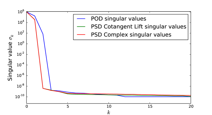
Figure 3.1: The decay of the singular values as calculated for the empirical data with each of the SVD-based algorithms.

3.3 Reduced model simulations

To test the accuracy of the considered model reduction methods, we have compared the results of reduced model simulations to a full-scale reference solution. The reference solution for $\beta=6.0$ was calculated on the time interval $0\leq t\leq 1000$ in the same way as the empirical data in Section 3.2. Note that for this choice of $\beta$ the period of the reference solution is $T\approx 1.05$ (see (3.5)), and the considered time interval encompasses roughly 955 periods. The reduced models were solved numerically on the same time interval using the second-order explicit and implicit midpoint methods. Note that when applied to a Hamiltonian system, the implicit midpoint method is a symplectic integrator, while the explicit midpoint method is not (see, e.g., [14]). All simulations were carried out with the time step $\Delta t=0.0001$. The POD model (2.4) was solved for $K=5$ and $K=10$ (thus reducing the dimensionality of the problem from $2n=2000$ to 5 and 10, respectively). Similarly, the PSD model (2.7) was solved for $K=5$ and $K=10$, both for the cotangent lift and complex SVD algorithms, in both cases reducing the dimensionality to 10 and 20, respectively. The choice of $K$ is a compromise between the speed and the accuracy: the smaller $K$ the faster the computation, but also the larger the projection error. In practice, one may choose $K$ based on the initial value of the error (3.8), i.e., the value of the projection error for the initial condition. For instance, in our experiment, the initial relative error for the POD simulations was equal to $1.09\cdot 10^{-14}$ for $K=5$, and $7.81\cdot 10^{-15}$ for $K=10$. All computations were performed in the Julia programming language with the help of the GeometricIntegrators.jl library (see [24]). The three main conclusions from the numerical experiments are described below.

Long-time instability of the POD simulations

As a measure of accuracy of the reduced models we take the relative error

$$\frac{\|u(t)-u_{\text{ref}}(t)\|}{\|u_{\text{ref}}(t)\|},$$ (3.8)

where $u_{\text{ref}}$ is the reference solution of (2.1), as described above, and $u=U_{K}\xi$ is the reconstructed solution, with $\xi$ being the numerical solution of the reduced model (2.4). The relative error as a function of time is depicted in Figure 3.2. We see that the POD simulations give very accurate results on shorter time intervals, but the errors blow up over a long integration time, and both the explicit and implicit midpoint method simulations become unstable. This is a consequence of the fact that there is no guarantee that the reduced system (2.4) retains any stability properties of the original system (2.1). In fact, the reduced equation for our example takes the form of the linear equation $\dot{\xi}=\Lambda_{K}\xi$, where the $K\times K$ matrix $\Lambda_{K}$ is given by

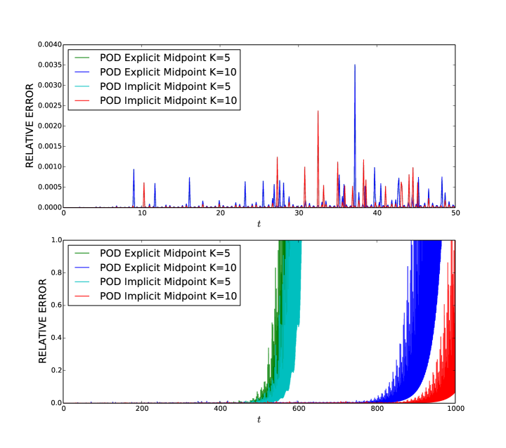
Figure 3.2: Top: The relative error of the POD simulations on the time interval $0\leq t\leq 50$. Both the explicit and implicit midpoint methods yield accurate approximations. Note that the plots for the explicit midpoint method with $K=5$ and $K=10$, as well as for the implicit midpoint method with $K=5$ and $K=10$, overlap very closely and are therefore indistinguishable. Bottom: The same plot over the whole simulation interval $0\leq t\leq 1000$. It is evident that over a long integration time the errors blow up and both the explicit and implicit method simulations become unstable.

$$\Lambda_{K}=U_{K}^{T}\left(\begin{matrix}0&\mathbb{I}_{n}\\ -\beta^{2}\mathbb{I}_{n}&0\end{matrix}\right)U_{K}.$$ (3.9)

In our experiment, for $K=5$ the matrix $\Lambda_{K}$ has 5 eigenvalues with positive real parts, the largest one of which equals $\text{Re}\,\lambda\approx 0.0655$. Similarly, for $K=10$ the eigenvalue with the largest real part is $\text{Re}\,\lambda\approx 0.0403$. The modes corresponding to these eigenvalues grow exponentially, and after a certain amount of time dominate the solution. This means that the reduced system is unstable; therefore, the errors arising from projecting the initial condition $\xi_{0}=U_{K}^{T}u_{0}$ and from applying numerical integration schemes amplify over the simulation time, eventually leading to the observed loss of accuracy (see [43], [45]).

Long-time stability of the PSD simulations

In the case of the PSD models the reconstructed solution $u=A\xi$ is obtained from the numerical solution $\xi$ of the reduced Hamiltonian system (2.7). The relative error as a function of time for the cotangent lift algorithm is depicted in Figure 3.3. We see that both the explicit and implicit midpoint methods retain good accuracy and stability over the whole integration time. It is therefore evident that by preserving the Hamiltonian structure of the particle equations, symplectic model reduction significantly improves the stability of the numerical computations even if a non-symplectic integrator (here the explicit midpoint method) is used. The numerical results for the complex SVD algorithm are nearly identical, therefore for brevity and clarity we skip presenting a separate figure.

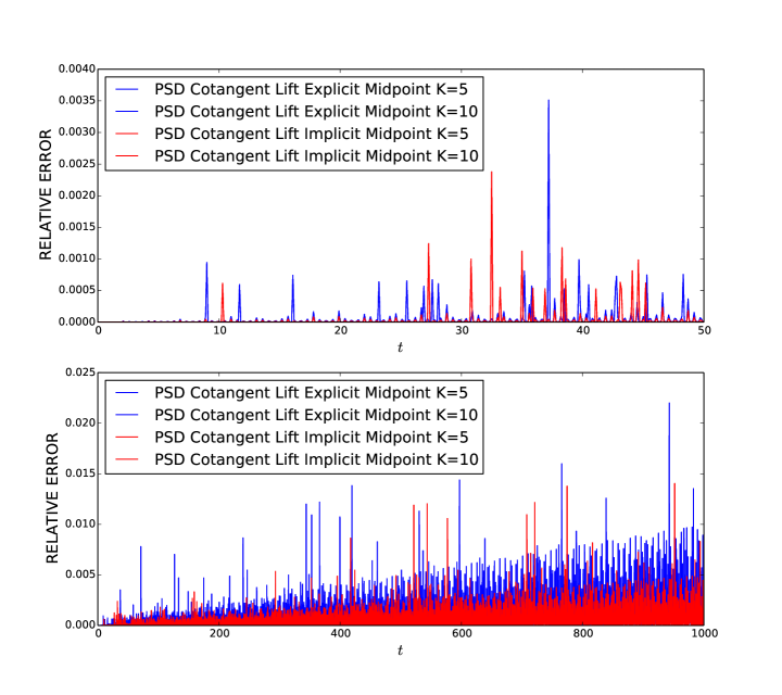
Figure 3.3: The relative error of the PSD simulations carried out with the cotangent lift algorithm on the time intervals $0\leq t\leq 50$ (Top) and $0\leq t\leq 1000$ (Bottom). The errors on the interval $0\leq t\leq 50$ are essentially identical for the POD and PSD simulations, but the PSD simulations retain good accuracy and stability over the whole integration time. The results for the complex SVD algorithm are nearly identical. Note that the same color code is used for the plots that overlap very closely and are therefore indistinguishable.

Long-time energy behavior

As the particle equations (1.1) are Hamiltonian, the total energy (1.5) of the particles should be preserved. In our numerical experiment the Hamiltonian for the reference solution (3.5) with $\beta=6.0$ was $H_{\text{ref}}\approx 1.803\cdot 10^{6}$. The relative error of the total energy of the particles for each of the algorithms is depicted in Figure 3.4 and Figure 3.5. One can clearly see that while the POD simulations initially retain the total energy relatively well, there is an evident linear growth trend for both the explicit and implicit midpoint methods, and the energy eventually blows up over a long integration time. On the other hand, the energy behavior for the PSD simulations is more stable. The non-symplectic explicit midpoint method applied to the cotangent lift algorithm also shows the same linear growth trend, but does not blow up. Furthermore, the implicit midpoint method, which is symplectic in this case, demonstrates near-preservation of the total energy, with only a minor linear growth throughout the whole simulation time. This demonstrates another important advantage of symplectic model reduction: since the reduced equations (2.7) are also Hamiltonian, one can employ symplectic time integrators to obtain a numerical solution that nearly conserves energy.

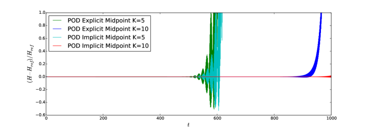
Figure 3.4: The relative error of the total energy of the particles as a function of time is depicted for the POD simulations. The energy eventually blows up for both the explicit and implicit midpoint methods.

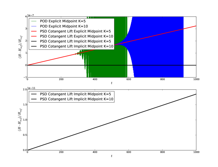
Figure 3.5: Top: The relative error of the total energy of the particles as a function of time is depicted for the PSD simulations. The energy behavior is more stable than for the POD simulations. While the non-symplectic explicit midpoint method shows a linear growth trend, the symplectic implicit midpoint method appears to nearly preserve the total energy. For comparison, also two POD simulations are depicted. Bottom: Same plot, but only the simulations for the symplectic implicit midpoint method are depicted in order to show the scale of energy preservation. In fact these simulations also show a linear trend, which is nevertheless four orders of magnitude smaller than for the non-symplectic explicit midpoint method. Note that the same color code is used for the plots that overlap very closely and are therefore indistinguishable. The results for the complex SVD algorithm are nearly identical, and are therefore omitted for clarity.

4 Summary and future work

We have compared several model reduction techniques and demonstrated their usefulness for particle-based simulations of the Vlasov equation. We have pointed out the importance of retaining the Hamiltonian structure of the equations governing the evolution of particles. Our work can be extended in several directions. First, model reduction methods can be applied to the Vlasov equation coupled to a self-consistent electric field satisfying the Poisson equation, or electromagnetic fields satisfying the Maxwell equations (see [23]). Second, model reduction of collisional Vlasov equations stemming from metriplectic brackets (see [18]) or stochastic action principles (see [25], [49], [50]) would be an interesting and useful extension of the work presented here.

References

- [1] B. Afkham and J. Hesthaven. Structure preserving model reduction of parametric Hamiltonian systems. SIAM Journal on Scientific Computing, 39(6):A2616–A2644, 2017.
- [2] B. M. Afkham, A. Bhatt, B. Haasdonk, and J. S. Hesthaven. Symplectic model-reduction with a weighted inner product. Unpublished, arXiv:1803.07799, 2018.
- [3] B. M. Afkham and J. S. Hesthaven. Structure-preserving model-reduction of dissipative Hamiltonian systems. Journal of Scientific Computing, 81:3–21, 2019.
- [4] A. Alla and J. N. Kutz. Nonlinear model order reduction via dynamic mode decomposition. SIAM Journal on Scientific Computing, 39(5):B778–B796, 2017.
- [5] A. C. Antoulas, D. C. Sorensen, and S. Gugercin. A survey of model reduction methods for large-scale systems. Contemporary Mathematics, 280:193–219, 2001.
- [6] P. Buchfink, A. Bhatt, and B. Haasdonk. Symplectic model order reduction with non-orthonormal bases. Mathematical and Computational Applications, 24:43, 2019.
- [7] A. Buffa, Y. Maday, A. T. Patera, C. Prud´homme, and G. Turinici. A priori convergence of the greedy algorithm for the parametrized reduced basis method. ESAIM: M2AN, 46(3):595–603, 2012.
- [8] K. Carlberg. Adaptive h-refinement for reduced-order models. International Journal for Numerical Methods in Engineering, 102(5):1192–1210, 2015.
- [9] K. Carlberg, R. Tuminaro, and P. Boggs. Preserving Lagrangian structure in nonlinear model reduction with application to structural dynamics. SIAM Journal on Scientific Computing, 37(2):B153–B184, 2015.
- [10] T. F. Chan and P. C. Hansen. Computing truncated singular value decomposition least squares solutions by rank revealing QR-factorizations. SIAM Journal on Scientific and Statistical Computing, 11(3):519–530, 1990.
- [11] S. Chaturantabut, C. Beattie, and S. Gugercin. Structure-preserving model reduction for nonlinear port-Hamiltonian systems. SIAM Journal on Scientific Computing, 38(5):B837–B865, 2016.
- [12] S. Chaturantabut and D. C. Sorensen. Nonlinear model reduction via discrete empirical interpolation. SIAM Journal on Scientific Computing, 32(5):2737–2764, 2010.
- [13] P. Drineas, R. Kannan, and M. W. Mahoney. Fast Monte Carlo algorithms for matrices II: Computing a low-rank approximation to a matrix. SIAM Journal on Computing, 36(1):158–183, 2006.
- [14] E. Hairer, C. Lubich, and G. Wanner. Geometric Numerical Integration: Structure-Preserving Algorithms for Ordinary Differential Equations. Springer Series in Computational Mathematics. Springer, New York, 2002.
- [15] N. Halko, P. G. Martinsson, and J. A. Tropp. Finding structure with randomness: Probabilistic algorithms for constructing approximate matrix decompositions. SIAM Review, 53(2):217–288, 2011.
- [16] J. Hall and M. Leok. Spectral variational integrators. Numer. Math., 130(4):681–740, Aug 2015.
- [17] J. Hesthaven, C. Pagliantini, and N. Ripamonti. Structure-preserving model order reduction of Hamiltonian systems. Unpublished, arXiv:2109.12367, 2021.
- [18] E. Hirvijoki, M. Kraus, and J. W. Burby. Metriplectic particle-in-cell integrators for the Landau collision operator. Preprint arXiv:1802.05263, 2018.
- [19] D. D. Holm, T. Schmah, and C. Stoica. Geometric Mechanics and Symmetry: From Finite to Infinite Dimensions. Oxford Texts in Applied and Engineering Mathematics. Oxford University Press, Oxford, 2009.
- [20] J. Jackson. Classical Electrodynamics, 3rd ed. John Wiley & Sons, New York, 1999.
- [21] C. Kane, J. E. Marsden, M. Ortiz, and M. West. Variational integrators and the Newmark algorithm for conservative and dissipative mechanical systems. International Journal for Numerical Methods in Engineering, 49(10):1295–1325, 2000.
- [22] M. Kraus. Variational integrators in plasma physics. PhD thesis, Technische Universität München, 2013.
- [23] M. Kraus, K. Kormann, P. Morrison, and E. Sonnendrücker. GEMPIC: geometric electromagnetic particle-in-cell methods. Journal of Plasma Physics, 83(4):905830401, 2017.
- [24] M. Kraus, T. Tyranowski, C. Albert, and C. Rackauckas. DDMGNI/GeometricIntegrators.jl: v0.2.0, Feb. 2020. https://doi.org/10.5281/zenodo.3648326.
- [25] M. Kraus and T. M. Tyranowski. Variational integrators for stochastic dissipative Hamiltonian systems. IMA Journal of Numerical Analysis, 41(2):1318–1367, 2020.
- [26] K. Kunisch and S. Volkwein. Galerkin proper orthogonal decomposition methods for a general equation in fluid dynamics. SIAM Journal on Numerical Analysis, 40(2):492–515, 2002.
- [27] S. Lall, P. Krysl, and J. E. Marsden. Structure-preserving model reduction for mechanical systems. Physica D: Nonlinear Phenomena, 184(1):304–318, 2003. Complexity and Nonlinearity in Physical Systems – A Special Issue to Honor Alan Newell.
- [28] T. Lassila, A. Manzoni, A. Quarteroni, and G. Rozza. Model Order Reduction in Fluid Dynamics: Challenges and Perspectives, pages 235–273. Springer International Publishing, 2014.
- [29] M. Leok and J. Zhang. Discrete Hamiltonian variational integrators. IMA Journal of Numerical Analysis, 31(4):1497–1532, 2011.
- [30] J. Marsden and T. Ratiu. Introduction to Mechanics and Symmetry, volume 17 of Texts in Applied Mathematics. Springer Verlag, 1994.
- [31] J. E. Marsden, G. W. Patrick, and S. Shkoller. Multisymplectic geometry, variational integrators, and nonlinear PDEs. Communications in Mathematical Physics, 199(2):351–395, 1998.
- [32] J. E. Marsden and M. West. Discrete mechanics and variational integrators. Acta Numerica, 10(1):357–514, 2001.
- [33] R. I. McLachlan and G. R. W. Quispel. Geometric integrators for ODEs. Journal of Physics A: Mathematical and General, 39(19):5251–5285, 2006.
- [34] B. Moore. Principal component analysis in linear systems: Controllability, observability, and model reduction. IEEE Transactions on Automatic Control, 26(1):17–32, 1981.
- [35] S. Ober-Blöbaum and N. Saake. Construction and analysis of higher order Galerkin variational integrators. Advances in Computational Mathematics, 41(6):955–986, 2015.
- [36] M. Ohlberger and S. Rave. Reduced basis methods: Success, limitations and future challenges. Proceedings of the Conference Algoritmy, pages 1–12, 2016.
- [37] C. Pagliantini. Dynamical reduced basis methods for Hamiltonian systems. Numerische Mathematik, 148(2):409–448, 2021.
- [38] B. Peherstorfer and K. Willcox. Online adaptive model reduction for nonlinear systems via low-rank updates. SIAM Journal on Scientific Computing, 37(4):A2123–A2150, 2015.
- [39] L. Peng and K. Mohseni. Geometric model reduction of forced and dissipative Hamiltonian systems. In 2016 IEEE 55th Conference on Decision and Control (CDC), pages 7465–7470, 2016.
- [40] L. Peng and K. Mohseni. Structure-preserving model reduction of forced Hamiltonian systems. Unpublished, arXiv:1603.03514, 2016.
- [41] L. Peng and K. Mohseni. Symplectic model reduction of Hamiltonian systems. SIAM Journal on Scientific Computing, 38(1):A1–A27, 2016.
- [42] A. Pinkus. N-widths in Approximation Theory. Ergebnisse der Mathematik und ihrer Grenzgebiete : a series of modern surveys in mathematics. Folge 3. Springer-Verlag, 1985.
- [43] S. Prajna. POD model reduction with stability guarantee. In 42nd IEEE International Conference on Decision and Control (IEEE Cat. No.03CH37475), volume 5, pages 5254–5258 Vol.5, 2003.
- [44] H. Qin, J. Liu, J. Xiao, R. Zhang, Y. He, Y. Wang, Y. Sun, J. W. Burby, L. Ellison, and Y. Zhou. Canonical symplectic particle-in-cell method for long-term large-scale simulations of the Vlasov–Maxwell equations. Nuclear Fusion, 56(1):014001, 2016.
- [45] M. Rathinam and L. R. Petzold. A new look at proper orthogonal decomposition. SIAM Journal on Numerical Analysis, 41(5):1893–1925, 2003.
- [46] C. W. Rowley and J. E. Marsden. Variational integrators for degenerate Lagrangians, with application to point vortices. In Decision and Control, 2002, Proceedings of the 41st IEEE Conference on, volume 2, pages 1521–1527. IEEE, 2002.
- [47] J. M. Sanz-Serna. Symplectic integrators for Hamiltonian problems: an overview. Acta Numerica, 1:243–286, 1992.
- [48] T. M. Tyranowski. Geometric integration applied to moving mesh methods and degenerate Lagrangians. PhD thesis, California Institute of Technology, 2014.
- [49] T. M. Tyranowski. Stochastic variational principles for the collisional Vlasov-Maxwell and Vlasov-Poisson equations. Proceedings of the Royal Society A: Mathematical, Physical and Engineering Sciences, 477(2252):20210167, 2021.
- [50] T. M. Tyranowski. Data-driven structure-preserving model reduction for stochastic Hamiltonian systems. Preprint arXiv:2201.13391, 2022.
- [51] T. M. Tyranowski and M. Desbrun. R-adaptive multisymplectic and variational integrators. Mathematics, 7(7), 2019.
- [52] T. M. Tyranowski and M. Desbrun. Variational partitioned Runge-Kutta methods for Lagrangians linear in velocities. Mathematics, 7(9), 2019.
- [53] J. Xiao, J. Liu, H. Qin, and Z. Yu. A variational multi-symplectic particle-in-cell algorithm with smoothing functions for the Vlasov-Maxwell system. Physics of Plasmas, 20(10):102517, 2013.
- [54] J. Xiao, H. Qin, and J. Liu. Structure-preserving geometric particle-in-cell methods for Vlasov-Maxwell systems. Plasma Science and Technology, 20(11):110501, sep 2018.
- [55] J. Xiao, H. Qin, J. Liu, Y. He, R. Zhang, and Y. Sun. Explicit high-order non-canonical symplectic particle-in-cell algorithms for Vlasov–Maxwell systems. Physics of Plasmas, 22:112504, 2015.