Charmonium spectroscopy motivated by general features of pNRQCD

Abstract

Mass spectrum of charmonium is computed in the framework of potential non-relativistic quantum chromodynamics. O$(1/m)$ and O$(1/m^{2})$ relativistic corrections to the Cornell potential and spin-dependent potential have been added, and is solved numerically. New experimentally observed and modified positive and negative parity states like ${{\boldsymbol{\psi}}{(4230)}}$, ${{\boldsymbol{\psi}}{(4260)}}$, ${{\boldsymbol{\psi}}{(4360)}}$, ${{\boldsymbol{\psi}}{(4390)}}$, ${{\boldsymbol{\psi}}{(4660)}}$, ${{\boldsymbol{\chi}}_{{c1}}{(4140)}}$ and ${{\boldsymbol{\chi}}_{{c1}}{(4274)}}$ near open-flavor threshold have also been studied. We explain them as admixtures of S-D wave states and P-wave states. Apart from these states, some other states like ${{\mathit{X}}{(3915)}}$, ${{\boldsymbol{\chi}}_{{c1}}{(3872)}}$, ${{\boldsymbol{\psi}}{(3770)}}$ and ${{\boldsymbol{\psi}}{(4160)}}$ have been identified as $2^{3}P_{0}$, $2^{3}P_{1}$, $1^{3}D_{1}$ and $2^{3}D_{1}$ states. Subsequently, the electromagnetic transition widths and $\gamma\gamma$, $e^{+}e^{-}$, light hadron and $\gamma\gamma\gamma$ decay widths of several states are calculated at various leading orders. All the calculated results are compared with experimental and results from various theoretical models.

1 Introduction

Remarkable experimental progress has been made in recent years in the field of heavy flavour hadrons specially charmonia. All the narrow charmonium states below open charm threshold($D\bar{D}$) have been observed experimentally and they have been successfully studied theoretically by many approaches like lattice QCD McNeile:2012qf , chiral perturbation theory Gasser:1983yg , heavy quark effective field theory Neubert:1993mb , QCD sum rules Veliev:2010vd , NRQCD Bodwin:1994jh , dynamical equations based approaches like
Schwinger-Dyson and Bethe-Salpeter equations(BSE) LlewellynSmith:1969az ; Mitra:2001ns ; Ricken:2000kf ; Mitra:1990av and some potential models Vinodkumar:1999da ; Pandya:2001hx ; KumarRai:2005yr ; Rai:2006bt ; Rai:2006wm ; Pandya:2008vf ; Vinodkumar:2008zd ; Rai:2008zza ; Pandya:2014qma . However, there are many questions related to charmonium physics in the region above $D\bar{D}$ threshold. $X$ and $Y$ states above $D\bar{D}$ threshold have been reported with unusual properties which are yet to be explained completely. These states however could be exotic states, mesonic molecules multi quark states or even admixtures of lower lying charmonia states which have been broadly put forward in Brambilla:2010cs and references therein. Charmoniumlike states having normal quantum numbers have similar masses when compared to normal charmonium, thus in order to study and understand the nature of higher mass states near $D\bar{D}$ threshold it is necessary to have better understanding of lower lying charmonium states.
Formerly ${{\mathit{X}}{(3872)}}$ (Now, ${{\boldsymbol{\chi}}_{{c1}}{(3872)}}$) was studied for the first time at Belle Choi:2003ue in $2003$ in exclusive decay of ${{\mathit{B}}^{\pm}}$ which was later produced by ${{\mathit{p}}^{+}}{{\mathit{p}}^{-}}$ collision Acosta:2003zx as well. Successively ${{\mathit{X}}{(3872)}}$ was studied theoretical as exotic state by Braaten:2018eov ; Kalashnikova_2019, as pure chamonium state by Swanson:2004pp ; Hanhart:2007yq ; Aceti:2012cb , as meson-meson molecular structure by Swanson:2004pp ; Hanhart:2007yq ; Aceti:2012cb , as tetra-quark state and as charmonia core plus higher fock components due to coupling to meson meson continuum by Ferretti:2013faa ; Barnes:2005pb ; Pennington:2007xr ; Danilkin:2010cc ; Karliner:2014lta ; Cardoso:2014xda ; Badalian:2015dha . Recently in PDG Tanabashi:2018oca ${{\mathit{X}}{(3872)}}$ was renamed ${{\boldsymbol{\chi}}_{{c1}}{(3872)}}$ considering it as a potential charmonium candidate and theoretically supported by Kher:2018wtv as pure charmonium candidate. Also CDF collaboration Abulencia:2006ma explained ${{\mathit{X}}{(3872)}}$ particle as a conventional charmonium state with J^PC $1^{++}$ or $2^{-+}$.
${{\boldsymbol{\chi}}_{{c1}}{(4140)}}$ previously known as ${{\boldsymbol{X}}{(4140)}}$ or ${{\boldsymbol{Y}}{(4140)}}$ discovered by CDF Aaltonen:2009tz ; Aaltonen:2011at in $2008$ near ${\boldsymbol{J}/\psi\phi}$ threshold, was later confirmed by D0 and CMS Abazov:2013xda ; Chatrchyan:2013dma . The result of the state was negative in B decays at Belle Brodzicka:2010zz ; Shen:2009vs , LHCb Aaij:2012pz and BABAR Lees:2014lra . The CDF collaboration in $2011$ observed ${{\mathit{X}}{(4140)}}$ with statistical significance greater than 5 standard deviations and also found evidence for another state ${{\boldsymbol{X}}{(4274)}}$ now known as ${{\boldsymbol{\chi}}_{{c1}}{(4274)}}$ with mass $4274.4{}^{+8.4}_{-6.7}\pm 1.9$ MeV Aaltonen:2011at . LHCb in $2017$ confirmed ${{\boldsymbol{\chi}}_{{c1}}{(4140)}}$ and ${{\boldsymbol{\chi}}_{{c1}}{(4274)}}$ with masses $4146.5\pm 4.5{}^{+4.6}_{-2.8}$ and $4273.3\pm 8.3{}^{+17.2}_{-3.6}$ MeV respectively. Both having $J^{PC}=1^{--}$ as reported by Tanabashi:2018oca . ${{\boldsymbol{X}}{(4140)}}$ has been studied by many theoretical studies as a molecular state, tetra-quark state or a hybrid state Liu:2009ei ; Branz:2009yt ; Albuquerque:2009ak ; Ding:2009vd ; Stancu:2009ka ; Wang:2015pea ; Anisovich:2015caa ; Wang:2009ue ; Mahajan:2009pj . Lu:2016cwr has suggested ${{\boldsymbol{X}}{(4274)}}$ to be ${\boldsymbol{\chi}}_{c1}3^{3}P_{1}$ state, Bhavsar:2018umj has studied ${{\boldsymbol{\chi}}_{{c1}}{(4140)}}$ as an admixture of P wave states.
${{\mathit{X}}{(3915)}}$ formerly ${{\boldsymbol{\chi}}_{{c0}}{(3915)}}$ was observed by Belle collaboration Uehara:2009tx with mass $3915\pm 3\pm 2$ MeV in photon-photon collision and experimental analysis Tanabashi:2018oca presented $\mathit{J}{}^{PC}=2{}^{++}$ for the same. This let to its assignment as $2^{3}P_{0}$ by Liu:2009fe and BABAR & SLAC Lees:2012xs , and $2^{3}P_{2}$ by Branz:2010rj .
${{\boldsymbol{\psi}}{(4230)}}$ previously known as ${{\mathit{X}}{(4230)}}$ first observed at BESIII Ablikim:2014qwy in $2015$ as one of the two resonant structure in ${{\mathit{e}}^{+}}{{\mathit{e}}^{-}}\rightarrow{{\boldsymbol{\omega}}}{{\boldsymbol{\chi}}_{{c0}}}$ with statistical significance more than $9\sigma$. Having $J^{PC}=1^{--}$ this state shows properties different from a conventional ${{\mathit{q}}}{{\overline{\mathit{q}}}}$ state and can be a candidate for an exotic structure.
${{\boldsymbol{\psi}}{(4390)}}$ formerly known as ${{\mathit{X}}{(4390)}}$ is the latest observed state at BESIII BESIII:2016adj in $2017$ during the process $e^{+}e^{-}\to\pi^{+}\pi^{-}h_{c}$, at center-of-mass energies from $3.896$ to $4.600$ GeV having mass $4391.5{}^{+6.3}_{-6.8}\pm 1.0$ MeV and $J^{PC}=1^{--}$. This state can also show property different from conventional charmonium state and has sparse theoretical and practical knowledge.
${{\boldsymbol{\psi}}{(4660)}}$ previously known as ${{\mathit{Y}}{(4660)}}$ discovered by Belle Wang:2007ea ; Wang:2014hta and confirmed by BaBar Lees:2012pv and having negative parity.
${{\boldsymbol{\psi}}{(3770)}}$ resonance is a vector state first detected at SPEAR Rapidis:1977cv in 1977, PDG Tanabashi:2018oca estimates its mass as $3773.13\pm 0.35$ MeV. Godfrey Godfrey:1985xj in $1985$ assigned it as $1^{3}D_{1}$ state.
${{\boldsymbol{\psi}}{(4160)}}$ having $J^{PC}=1^{--}$ first experiment evidence given by Brandelik:1978ei , recently observed by Belle Wang:2012bgc and LHCB PhysRevD.87.051101 in $2013$. PDG Tanabashi:2018oca estimates mass as $4191\pm 5$ MeV.
${{\mathit{Y}}{(4260)}}$ and ${{\mathit{Y}}{(4360)}}$ which have been renamed in PDG Tanabashi:2018oca as ${{\boldsymbol{\psi}}{(4260)}}$ and ${{\boldsymbol{\psi}}{(4360)}}$ were first observed at BABAR Aubert:2005rm in $2005$ and at Belle Wang:2007ea in $2007$ respectively. Both are vector states, yet unlike most conventional charmonium do not corresponds to enhancements in ${{\mathit{e}}^{+}}{{\mathit{e}}^{-}}$ hadronic cross section nor decay to $D\bar{D}$ but decay as $\pi^{+}\pi^{-}\boldsymbol{J}/\psi$ and $\pi^{+}\pi^{-}\boldsymbol{\psi}(2S)$ respectively. Both these states can have properties different from conventional charmonia state, Cleven:2013mka has considered ${{\mathit{Y}}{(4260)}}$ as a molecular structure. Recently these two states have been studied as S-D states admixtures in Bhavsar:2018umj as study of charmonium in relativistic Dirac formalism with linear confinement potential. The above mentioned states have been tabulated in Table1.
Charmomium is most dense system in the entire heavy flavor spectroscopy having $37$ experimentally discovered states. In phenomenology the charmonium mass spectrum is computed by many potential models like relativistic quark model Lakhina:2006vg , screened potential model Deng:2016stx ; Deng:2016ktl , constituent quark model Segovia:2016xqb and some non-linear potential models Patel:2015ywa ; Bonati:2015dka ; Gutsche:2014oua ; Shah:2012js ; Negash:2015rua ; Li:2009zu ; Li:2009nr ; Quigg:1977dd ; Martin:1980jx ; Buchmuller:1980su . Cornell potential is most commonly studied potential for heavy quarkonia system and has been supported by lattice QCD simulations as well Bali:1994de ; Bali:2000vr . Detailed explanation about quark model hypothesis has been discussed in Raghav:2018bqo . Quark model for studying heavy quarkonia has some common features when compared with QCD but it is not a complete QCD approach, hence most forms of QCD inspired potential would result in uncertainties in the computation of the spectroscopic properties particularly in the intermediate range. Different potential models may produce similar mass spectra matching with the experimentally determined masses but the decay properties mainly leptonic decays or radiative transitions are not in agreement with experimental values. Therefore, test for any model is to reproduce mass spectra along with decay properties. Here, we couple Cornell potential with non-relativistic effective field theory(pNRQCD) Brambilla:2004jw . The small velocity of charm quark in $c\bar{c}$ bound state enables us to use non-relativistic effective field theory within QCD to study charmonia. There are three well defined scales in heavy quarkonia namely; hard scale, soft scale and ultarsoft scale and they also follow a well defined pecking order $m_{Q}\gg mv\gg mv^{2}$, with $m\gg\Lambda_{QCD}$, $\Lambda_{QCD}$ is a QCD scale parameter. NRQCD cannot distinguish soft and ultrasoft scales, which complicates power counting. pNRQCD Pineda:1997bj ; Brambilla:1999xf solves this problem by integrating the energy scales above $mv$ in NRQCD. The above statements have been discussed in detail in previous work Raghav:2018bqo . Recently a study on Cornell Model calibration with NRQCD at $N^{3}LO$ has been done Ortega:2018oae . A spin dependent relativistic correction term (in the framework of pNRQCD koma ) has been added with Coulomb plus confinement potential in the present work, and the Schrödinger equation has been solved numerically Lucha:1998xc .
The theoretical framework has been discussed in Section 2, Various decays of S and P wave states has been discussed in Section 3, Charmoniumlike negative and positive parity states have been discussed in Section 4, Electromagnetic transition widths are in Section 5 and finally results, discussion and conclusion are presented in Sections 6 and 7.

Table 1: Experimental status of some negative and positive parity $c\bar{c}$ mesons near open-flavor threshold reported by PDGTanabashi:2018oca

. PDG Former/Common Expt.Mass J^P Production Discovery Name Name (in keV) Year ${{\boldsymbol{\psi}}{(3770)}}$ – 3773.13$\pm$0.35 $1^{-}$ ${{\mathit{e}}^{+}}{{\mathit{e}}^{-}}\rightarrow{{\mathit{D}}}{{\overline{\mathit{D}}}}$ 2012 ${{\boldsymbol{\chi}}_{{c1}}{(3872)}}$ ${{\mathit{X}}{(3872)}}$ 3871.69$\pm$0.17 $1^{+}$ ${{X\mathit{B}}}\rightarrow{{\mathit{K}}}{\pi}^{+}{\pi}^{-}{{\mathit{J}/\psi}{(1S)}}$ 2003 ${{\mathit{X}}{(3900)}}$ ${{\mathit{X}}{(3900)}}$ 3886.6$\pm$2.4 $1^{+}$ ${{\boldsymbol{\psi}}{(4260)}}\rightarrow{\pi}^{-}{{\mathit{X}}}$ 2013 ${{\mathit{X}}{(3915)}}$ ${{\boldsymbol{\chi}}_{{c0}}{(3915)}}$ 3918.4$\pm$1.9 $0^{+}or2^{+}$ ${{\mathit{e}}^{+}}{{\mathit{e}}^{-}}\rightarrow{{\mathit{e}}^{+}}{{\mathit{e}}^{-}}{{\mathit{X}}}$ 2004 ${{\boldsymbol{\chi}}_{{c1}}{(4140)}}$ ${{\mathit{X}}{(4140)}}$ 4146.8$\pm$2.4 $1^{+}$ ${{\mathit{B}}^{+}}\rightarrow{{\boldsymbol{\chi}}_{{c1}}}{{\mathit{K}}^{+}}$ 2008 ${{\mathit{e}}^{+}}{{\mathit{e}}^{-}}\rightarrow{{\mathit{e}}^{+}}{{\mathit{e}}^{-}}{{\mathit{X}}}$ ${{\boldsymbol{\psi}}{(4160)}}$ – 4191$\pm$5 $1^{-}$ ${{\mathit{e}}^{+}}{{\mathit{e}}^{-}}\rightarrow{{\mathit{J}/\psi}}{{\mathit{X}}}$ 2007 ${{\boldsymbol{\psi}}{(4230)}}$ ${{\mathit{X}}{(4230)}}$ $4218{}^{+5}_{-4}$ $1^{-}$ ${{\mathit{e}}^{+}}{{\mathit{e}}^{-}}\rightarrow{{\mathit{X}}}$ 2015 ${{\boldsymbol{\psi}}{(4260)}}$ ${{\mathit{Y}}{(4260)}}$ 4230$\pm$8 $1^{-}$ ${{\mathit{e}}^{+}}{{\mathit{e}}^{-}}\rightarrow{{\mathit{X}}}$ 2005 ${{\mathit{X}}{(4260)}}$ ${{\boldsymbol{\chi}}_{{c1}}{(4274)}}$ ${{\mathit{X}}{(4274)}}$ $4274{}^{+8}_{-6}$ $1^{+}$ ${{\mathit{B}}^{+}}\rightarrow{{\mathit{K}}^{+}}{{\mathit{X}}}$ 2011 ${{\boldsymbol{\psi}}{(4360)}}$ ${{\mathit{Y}}{(4360)}}$ 4368$\pm$13 $1^{-}$ ${{\mathit{e}}^{+}}{{\mathit{e}}^{-}}\rightarrow{{\mathit{X}}}$ 2007 ${{\boldsymbol{\psi}}{(4390)}}$ ${{\mathit{X}}{(4390)}}$ 4392$\pm$7 $1^{-}$ ${{\mathit{e}}^{+}}{{\mathit{e}}^{-}}\rightarrow{{\mathit{X}}}$ 2017 ${{\boldsymbol{\psi}}{(4660)}}$ ${{\mathit{Y}}{(4660)}}$ $4643\pm 9$ $1^{-}$ ${{\mathit{e}}^{+}}{{\mathit{e}}^{-}}\rightarrow{{\mathit{X}}}$ 2007

2 Theoretical framework

Considering charmonium as non-relativistic system we use the following Hamiltonian to calculate its mass spectra. Same theoretical framework has been used by us for studding bottomonium in effective filed theory formalismRaghav:2018bqo .

$$H=M+\frac{P^{2}}{2\mu}+V_{pNRQCD}(r)+V_{SD}(r)$$ (1)

Here, $M$ and $\mu$ represents the total and the reduced mass of the system. Three terms namely Coulombic term $V_{v}$(r) (vector), a confinement term $V_{s}$ (scalar) and relativistic correction $V_{p}(r)$ in the framework of pNRQCDBrambilla:2000gk ; article ; Raghav:2018bqo ; PerezNadal:2008vm has been included in the interaction potential $V_{pNRQCD}(r)$. After fitting the spin average ground state mass(1S) with its experimental value, we fix the mass of charm quark and other potential parameters like $\epsilon$, $A$, $\alpha_{s}$, $\sigma$, $C$ and $a$, there values are given in Table 2, With these parameters, $\chi^{2}$/d.o.fHuang:2019agb is estimated to be $1.553$. Using these fixed values we generate the entire mass spectrum of charmonium by solving the Schrödinger equation numerically Lucha:1998xc .

$$V_{pNRQCD}(r) = V_{v}(r)+V_{s}(r)+V_{p}(r)$$ (2)

$$V_{pNRQCD}(r) = -\frac{4\alpha_{s}}{3r}+Ar+\frac{1}{m_{c}}V^{(1)}(r)+\frac{1}{m_{c}^{2}}V^{(2)}(r)$$ (3)

$$V^{(1)}(r)=-\frac{9\alpha_{c}^{2}}{8r^{2}}+a\log r+C$$ (4)

The parameter $A$ represents potential strength analogous to spring tension. $\alpha_{s}$ and $\alpha_{c}$ are strong and effective running coupling constants respectively, $m_{c}$ is mass of charm quark, $a$ and $C$ are potential parameters. Spin-dependent part of the usual one gluon exchange potential has been considered to obtain mass difference between degenerate mesonic states,

$$V^{(2)}(r) = V_{SS}(r)\bigg{[}S(S+1)-\frac{3}{2}\bigg{]}+V_{L\cdot S}(r)(\overrightarrow{L}\cdot\overrightarrow{S})$$ (6)

$$+V_{T}(r)\bigg{[}S(S+1)-3(S\cdot\hat{r})(S\cdot\hat{r})\bigg{]}$$

Where the spin-spin interaction

$$V_{SS}(r)=\frac{8}{9}\frac{\alpha_{s}}{m_{c}^{2}}\overrightarrow{S}_{Q}\overrightarrow{S}_{\bar{Q}}4\pi\delta^{3}(\vec{r}),$$ (7)

and the spin-orbital interaction

$$V_{L.S}(r) = \frac{1}{m_{c}^{2}}\bigg{(}\frac{C_{s}}{2r}\frac{d}{dr}(V_{v}(r)+V_{s}(r))$$ (9)

$$+\frac{C_{f}}{r}\left[-\left(1-\epsilon\right)A+\left(\frac{\alpha_{c}}{r^{2}}+\epsilon A\right)\right]\bigg{)}$$

with $C_{f}=\frac{4}{3}$, and the tensor interaction

$$V_{T}(r) = \frac{1}{m_{c}^{2}}\frac{{C_{f}}^{2}}{3}\frac{3\alpha}{r^{3}}$$ (10)

Table 2: Potential parameters

$\alpha_{c}$	$m_{c}$	$\epsilon$	A	$\alpha_{s}$	C	a
0.4	1.321GeV	0.12	0.191 $\frac{GeV}{fm}$	0.318	0.12	-0.165 ${GeV}^{2}$
			$\chi^{2}$/d.o.f=1.553

Here, the effect of relativistic corrections, the ${\cal O}\left(1/m\right)$ correction, the spin-spin, spin-orbit and tensor corrections ${\cal O}\left(1/m^{2}\right)$ are tested for charmonium.
The computed masses of $S$, $P$, $D$ and $F$ states are tabulated in Tables 3 and 4, along with latest experimental data and other theoretical approaches and is found to be in good agreement with them.

Table 3: S and P state mass spectra of $c\bar{c}$ meson (in GeV)

State	Present	Tanabashi:2018oca	Chaturvedi:2018xrg	Ebert:2011jc	Sultan:2014oua	Soni:2017wvy	LQCDKalinowski:2015bwa
$1^{1}S_{0}$	2.989	2.984$\pm$0.005	3.004	2.981	2.982	2.989	2.884
$1^{3}S_{1}$	3.094	3.097$\pm$0.006	3.086	3.096	3.090	3.094	3.056
$2^{1}S_{0}$	3.572	3.639$\pm$0.012	3.645	3.635	3.630	3.602	3.535
$2^{3}S_{1}$	3.649	3.686$\pm$0.025	3.708	3.685	3.672	3.681	3.662
$3^{1}S_{0}$	3.998	–	3.989	4.043	4.058	–	–
$3^{3}S_{1}$	4.062	4.039$\pm$0.043	4.039	4.072	4.129	–	–
$4^{1}S_{0}$	4.372	–	4.534	4.401	4.384	4.448	–
$4^{3}S_{1}$	4.428	4.421$\pm$0.004	4.579	4.427	4.406	4.514	–
$5^{1}S_{0}$	4.714	–	4.901	4.811	4.685	4.799	–
$5^{3}S_{1}$	4.763	–	4.942	4.837	4.704	4.863	–
$6^{1}S_{0}$	5.033	–	5.240	5.151	4.960	5.124	–
$6^{3}S_{1}$	5.075	–	5.277	5.167	4.977	5.185	–
$1^{3}P_{0}$	3.473	3.414$\pm$0.031	3.440	3.413	3.424	3.428	3.421
$1^{3}P_{1}$	3.506	3.510$\pm$0.007	3.492	3.511	3.505	3.468	3.480
$1^{1}P_{1}$	3.527	3.525$\pm$0.038	3.496	3.525	3.516	3.470	3.494
$1^{3}P_{2}$	3.551	3.556$\pm$0.007	3.511	3.555	3.549	3.480	3.536
$2^{3}P_{0}$	3.918	3.918 $\pm$0.019⋆	3.932	3.870	3.852	3.897	–
$2^{3}P_{1}$	3.949	3.871 $\pm$0.001⋆	3.984	3.906	3.925	3.938	–
$2^{1}P_{1}$	3.975	–	3.991	3.926	3.934	3.943	–
$2^{3}P_{2}$	4.002	3.927$\pm$.026	4.007	3.949	3.965	3.955	–
$3^{3}P_{0}$	4.306	–	4.394	4.301	4.202	4.296	–
$3^{3}P_{1}$	4.336	–	4.401	4.319	4.271	4.338	–
$3^{1}P_{1}$	4.364	–	4.410	4.337	4.279	4.344	–
$3^{3}P_{2}$	4.392	–	4.427	4.354	4.309	4.358	–
$4^{3}P_{0}$	4.659	–	4.722	4.698	4.509	4.653	–
$4^{3}P_{1}$	4.688	–	4.771	4.728	4.576	4.696	–
$4^{1}P_{1}$	4.716	–	4.784	4.744	4.585	4.704	–
$4^{3}P_{2}$	4.744	–	4.802	4.763	4.614	4.718	–

Table 4: D and F wave mass spectra of $c\bar{c}$ meson (in GeV)

State		Tanabashi:2018oca	Chaturvedi:2018xrg	Ebert:2011jc	Sultan:2014oua	Soni:2017wvy
$1^{3}D_{3}$	3.806	–	3.798	3.813	3.805	3.755
$1^{3}D_{2}$	3.800	3.822$\pm$0.012 Bhardwaj:2013rmw	3.814	3.795	3.800	3.772
$1^{3}D_{1}$	3.785	3.773$\pm$0.035⋆	3.815	3.783	3.785	3.775
$1^{1}D_{2}$	3.780	–	3.806	3.807	3.799	3.765
$2^{3}D_{3}$	4.206	–	4.273	4.220	4.165	4.176
$2^{3}D_{2}$	4.203	–	4.248	4.190	4.158	4.188
$2^{3}D_{1}$	4.196	4.191$\pm$0.005⋆	4.245	4.105	4.141	4.188
$2^{1}D_{2}$	4.203	–	4.242	4.196	4.158	4.182
$3^{3}D_{3}$	4.568	–	4.626	4.574	4.481	4.549
$3^{3}D_{2}$	4.566	–	4.632	4.544	4.472	4.557
$3^{3}D_{1}$	4.562	–	4.627	4.507	4.455	4.555
$3^{1}D_{2}$	4.566	–	4.629	4.549	4.472	4.553
$4^{3}D_{3}$	4.902	–	4.920	–	–	4.890
$4^{3}D_{2}$	4.901	–	4.896	–	–	4.896
$4^{3}D_{1}$	4.898	–	4.857	–	–	4.891
$4^{1}D_{2}$	4.901	–	4.898	–	–	4.892
$1^{3}F_{2}$	4.015	–	4.041	–	–	3.990
$1^{3}F_{3}$	4.039	–	4.068	–	–	4.012
$1^{3}F_{4}$	4.052	–	4.093	–	–	4.036
$1^{1}F_{3}$	4.039	–	4.071	–	–	4.017
$2^{3}F_{2}$	4.403	–	4.361	–	–	4.378
$2^{3}F_{3}$	4.413	–	4.400	–	–	4.396
$2^{3}F_{4}$	4.418	–	4.434	–	–	4.415
$2^{1}F_{3}$	4.413	–	4.406	–	–	4.400
$3^{3}F_{2}$	4.751	–	–	–	–	4.730
$3^{3}F_{3}$	4.756	–	–	–	–	4.746
$3^{3}F_{4}$	4.759	–	–	–	–	4.761
$3^{1}F_{3}$	4.756	–	–	–	–	4.749

3 Decay Widths of $S$ and $P$ charmoium states using NRQCD approach

Successful determination of decay widths along with the mass spectrum calculation is very important for believability of any potential model. Better insight into quark gluon dynamics can be provided by studding strong decays, radiative decays and leptonic decays of vector mesons. Determined radial wave functions and extracted model parameters are utilized to compute various decay widths. The short distance and long distance factors in NRQCD are calculated in terms of running coupling constant and non-relativistic wavefunction.

3.1 $\gamma\gamma$ decay width

The $\gamma\gamma$ decay widths of $S$-wave states have been calculated at NNLO in $\nu$, at NLO in $\nu^{2}$, at $O(\alpha_{s}\nu^{2})$ and at NLO in $\nu^{4}$. NRQCD factorization expression for the decay widths of quarkonia at NLO in $\nu^{4}$ is given asBraaten:1995ej

$$\Gamma(^{1}S_{0}\rightarrow\gamma\gamma)=\frac{F_{\gamma\gamma}(^{1}S_{0})}{m^{2}_{Q}}\left|\left<0|\chi^{{\dagger}}\psi|^{1}S_{0}\right>\right|^{2}$$

$$+\frac{G_{\gamma\gamma}(^{1}S_{0})}{m^{4}_{Q}}Re\left[\left<{}^{1}S_{0}|\psi^{{\dagger}}\chi|0\right>\left<0|\chi^{{\dagger}}\left(-\frac{i}{2}\overrightarrow{D}\right)^{2}\psi|^{1}S_{0}\right>\right]$$

(11)

$$+\frac{H^{1}_{\gamma\gamma}(^{1}S_{0})}{m^{6}_{Q}}\left<{}^{1}S_{0}|\psi^{{\dagger}}\left(-\frac{i}{2}\overrightarrow{D}\right)^{2}\chi|0\right>\times$$

$$\left<0|\chi^{{\dagger}}\left(-\frac{i}{2}\overrightarrow{D}\right)^{2}\psi|^{1}S_{0}\right>+\frac{H^{2}_{\gamma\gamma}(^{1}S_{0})}{m^{6}_{Q}}\times$$

$$Re\left[\left<{}^{1}S_{0}|\psi^{{\dagger}}\chi|0\right>\left<0|\chi^{{\dagger}}\left(-\frac{i}{2}\overrightarrow{D}\right)^{4}\psi|^{1}S_{0}\right>\right]$$ (12)

The matrix elements that contribute to the decay rates of the S wave states to $\gamma\gamma$ are given as,

$$\left<{}^{1}S_{0}|{\cal{O}}(^{1}S_{0})|^{1}S_{0}\right>=\left|\left<0|\chi^{{\dagger}}\psi|^{1}S_{0}\right>\right|^{2}[1+O(v^{4}\Gamma)]$$

$$\left<{}^{3}S_{1}|{\cal{O}}(^{3}S_{1})|^{3}S_{1}\right>=\left|\left<0|\chi^{{\dagger}}\sigma\psi|^{3}S_{1}\right>\right|^{2}[1+O(v^{4}\Gamma)]$$

$$\left<{}^{1}S_{0}|{\cal{P}}_{1}(^{1}S_{0})|^{1}S_{0}\right>=Re\left[\left<{}^{1}S_{0}|\psi^{{\dagger}}\chi|0\right>\right.\times$$

$$\left.\left<0|\chi^{{\dagger}}(-\frac{i}{2}\overrightarrow{D})^{2}\psi|^{1}S_{0}\right>\right]+O(v^{4}\Gamma)$$ (13)

The matrix elements are expressed in terms of the regularized wave-function parametersBodwin:1994jh

$$\left<{}^{1}S_{0}|{\cal{O}}(^{1}S_{0})|^{1}S_{0}\right>=\frac{3}{2\pi}|R_{P}(0)|^{2}$$

$$\left<{}^{1}S_{0}|{\cal{P}}_{1}(^{1}S_{0})|^{1}S_{0}\right>=-\frac{3}{2\pi}|\overline{R^{*}_{P}}\ \overline{\bigtriangledown^{2}R_{P}}|$$

$$\left<{}^{1}S_{0}|{\cal{Q}}^{1}_{1}(^{1}S_{0})|^{1}S_{0}\right>=-\sqrt{\frac{3}{2\pi}}\overline{\nabla^{2}}R_{P}$$

From equation 3.1, for calculations at leading orders in $\nu$ only the first term is considered, for calculation at leading orders at $\nu^{2}$ the first two terms are considered, and for calculation at leading orders at $\nu^{4}$ all the terms are considered. The coefficients $F,G\&H$ are written asBrambilla:2010cs ; Bodwin:2002hg ; Feng:2015uha ; Brambilla:2018tyu ; Bodwin:1994jh ; Jia:2011ah

$$F_{\gamma\gamma}(^{1}S_{0})=2\pi Q^{4}\alpha^{2}\bigg{[}1+C_{F}{\alpha_{s}\over\pi}\left(\frac{\pi^{2}}{4}-5\right)$$

$$+C_{F}{\alpha_{s}^{2}\over\pi^{2}}\bigg{[}C_{F}\left(-21-\pi^{2}\left(\frac{1}{4\epsilon}+ln\frac{\mu}{m}\right)\right)+$$

$$C_{A}\left(-4.79-\frac{\pi^{2}}{2}\left(\frac{1}{4\epsilon}+ln\frac{\mu}{m}\right)\right)-$$

$$0.565N_{L}T_{R}+0.22N_{H}T_{R}\bigg{]}\bigg{]}$$ (15)

$$G_{\gamma\gamma}(^{1}S_{0})=-{8\pi Q^{4}\alpha^{2}\over 3}\bigg{[}1+{C_{F}\alpha_{s}\over\pi}$$ (16)

$$\bigg{(}{5\pi^{2}\over 16}-{49\over 12}-\ln{\mu^{2}\over 4m^{2}}\bigg{)}\bigg{]}$$

$$H_{\gamma\gamma}(^{1}S_{0})+H^{2}_{\gamma\gamma}(^{1}S_{0})=\frac{136\pi}{45}Q^{4}\alpha^{2}$$ (17)

Here, $C_{F}=4/3$, $C_{A}=3$, $N_{H}=1$, $T_{R}=1/2$, $N_{L}=3$ and $\mu=0.5$. For calculations at NNLO in $\nu$, the entire equation 3.1 is used. For calculations at NLO in $\nu^{2}$ only the first two terms in the square bracket of equation 3.1 is used, and $G_{\gamma\gamma}(^{1}S_{0})$ is taken as $-\frac{8\pi Q^{4}}{3}\alpha^{2}$. For NLO in $\nu^{4}$, in addition to first two terms in the square bracket of equation 3.1 and $G_{\gamma\gamma}(^{1}S_{0})=-\frac{8\pi Q^{4}}{3}\alpha^{2}$, equation 17 is also used. But, for calculation at $O(\alpha_{s}\nu^{2})$ the first two terms in square bracket of equation 3.1 and the entire equation 17 are only used. The calculated decay widths are tabulated in table5.

The decay widths for $n^{3}P_{J}(J=0,2)$ states to NLO in $\nu^{2}$ and NNLO in $\nu^{2}$ have also been calculated. $\gamma\gamma$ decay width of $n^{3}P_{0}$ and $n^{3}P_{2}$ is expressed as,

$$\Gamma(\chi_{cJ}\rightarrow\gamma\gamma) = \frac{3N_{c}ImF_{\gamma\gamma}(^{3}P_{J})}{\pi m_{Q}^{4}},\ \ \ J=0,2.$$ (18)

Short distance coefficients $F$’s, at NNLO in $\nu^{2}$ are given by Sang:2015uxg ; Bodwin:2002hg

$$F_{\gamma\gamma}(^{3}P_{0}) = 3\pi Q^{4}\alpha^{2}\bigg{[}1+C_{F}{\alpha_{s}\over\pi}\bigg{(}\frac{\pi^{2}}{4}-\frac{7}{3}\bigg{)}$$ (19)

$$+\frac{\alpha_{s}^{2}}{\pi^{2}}\bigg{[}C_{F}\frac{\beta_{0}}{4}\bigg{(}\frac{\pi^{2}}{4}-\frac{7}{3}\bigg{)}\ln\frac{\mu_{R}^{2}}{m^{2}}\bigg{]}\bigg{]}$$

$$F_{\gamma\gamma}(^{3}P_{2}) = \frac{4\pi Q^{4}\alpha^{2}}{5}\bigg{[}1-4C_{f}\frac{\alpha_{s}}{\pi}+$$ (20)

$$\frac{\alpha_{s}^{2}}{\pi^{2}}\bigg{(}-2C_{F}\frac{\beta_{0}}{4}\ln\frac{\mu_{R}^{2}}{m^{2}}\bigg{)}\bigg{]}$$

$\beta_{0}={11\over 3}C_{A}-{2\over 3}(n_{L}+n_{H})$ is the one-loop coefficient of the QCD $\beta$-function, where $n_{H}=1$, $C_{A}=3$ and $n_{L}$ signifies the number of light quark flavors ($n_{L}=3$ for $\chi_{c}$). The calculated decay widths are tabulated in table6.

Table 5: $\gamma\gamma$ decay widths of $n\eta_{c}$ meson(in keV)

$\Gamma$			State
	$1^{1}S_{0}$	$2^{1}S_{0}$	$3^{1}S_{0}$	$4^{1}S_{0}$	$5^{1}S_{0}$	$6^{1}S_{0}$
NNLO in $\nu$	12.4	8.257	7.102	6.474	6.093	5.788
NLO in $\nu^{2}$	14.129	9.273	6.238	4.674	3.747	3.125
$O(\alpha_{s}\nu^{2})$	14.897	9.734	6.547	4.906	3.933	3.280
NLO in $\nu^{4}$	6.725	3.178	1.493	0.858	0.560	0.394
Tanabashi:2018oca	5.05$\pm 0.01$	2.14$\pm$0.04
Chaturvedi:2018xrg	8.246	4.560	3.737	3.340	3.095	2.924
Soni:2017wvy	5.618	2.944	2.095	1.644	1.358	1.158
Lakhina:2006vg	7.18	1.71	1.21
Ebert:2002pp	5.5	1.8
Lansberg:2006dw	7.5-10
Kim:2004rz	7.14$\pm$0.95	4.4$\pm$0.48

Table 6: $\gamma\gamma$ decay widths of $n^{3}P_{J}(J=0,2)$ (in keV)

$\Gamma$		$\chi_{0}$				$\chi_{2}$
$\Gamma$	1P	2P	3P	4P	1P	2P	3P	4P
NLO in $\nu^{2}$	4.185	4.306	4.847	4.346	0.538	0.554	0.626	0.559
NNLO in $\nu^{2}$	4.134	4.263	4.799	4.303	0.868	0.893	1.005	0.901
Tanabashi:2018oca	2.341$\pm$0.189				0.528$\pm$0.404
Amsler:2008zzb	2.87$\pm$0.39				0.53$\pm$0.05
Chaturvedi:2018xrg	2.692	4.716	8.078	0.928	1.242	1.485	1.691	1.721
Hwang:2010iq	2.36$\pm$0.35				0.346$\pm$0.009	0.23
Gupta:1996ak	6.38				0.57
Huang:1996cs	3.72$\pm$1.1				0.490$\pm$0.150

3.2 $e^{+}e^{-}$ decay width

The $e^{+}e^{-}$ decay width of $S$-wave states have been calculated at NLO in $\nu$, NNLO in $\nu$, NLO in $\nu^{2}$, NLO in $\alpha_{s}\nu^{4}$ and NLO in $\alpha_{s}^{2}\nu^{4}$. NRQCD factorization expression for the decay widths of quarkonia at NNLO in $\nu^{4}$ is written as,

$$\Gamma(^{3}S_{1}\rightarrow e^{+}e^{-})=\frac{F_{ee}(^{3}S_{1})}{m^{2}_{Q}}\left|\left<0|\chi^{{\dagger}}\sigma\psi|^{3}S_{1}\right>\right|^{2}$$ (21)

$$+\frac{G_{ee}(^{3}S_{1})}{m^{4}_{Q}}Re\left[\left<{}^{3}S_{1}|\psi^{{\dagger}}\sigma\chi|0\right>\left<0|\chi^{{\dagger}}\sigma\left(-\frac{i}{2}\overrightarrow{D}\right)^{2}\psi|^{3}S_{1}\right>\right]$$ (22)

$$+\frac{H^{1}_{ee}\left({}^{1}S_{0}\right)}{m^{6}_{Q}}\left<{}^{3}S_{1}|\psi^{{\dagger}}\sigma\left(-\frac{i}{2}\overrightarrow{D}\right)^{2}\chi|0\right>\times$$

$$\left<0|\chi^{{\dagger}}\sigma\left(-\frac{i}{2}\overrightarrow{D}\right)^{2}\psi|^{3}S_{1}\right>+\frac{H^{2}_{ee}(^{1}S_{0})}{m^{6}_{Q}}\times$$

$$\ Re\left[\left<{}^{3}S_{1}|\psi^{{\dagger}}\sigma\chi|0\right>\left<0|\chi^{{\dagger}}\sigma\left(-\frac{i}{2}\overrightarrow{D}\right)^{4}\psi|^{3}S_{1}\right>\right]$$ (23)

From equation 21, for calculations at leading orders in $\nu$ only the first term is considered, for calculation at leading orders at $\nu^{2}$ the first two terms are considered, and for calculation at leading orders at $\nu^{4}$ all the terms are considered. The matrix elements that contribute to the decay rates of $\psi\rightarrow e^{+}e^{-}$ through the vacuum-saturation approximation gives Bodwin:1994jh .

$$\left<{}^{3}S_{1}|{\cal{P}}_{1}(^{3}S_{1})|^{3}S_{1}\right>=Re\left[\left<{}^{3}S_{1}|\psi^{{\dagger}}\sigma\chi|0\right>\right.\times$$

$$\left.\left<0|\chi^{{\dagger}}\times\sigma\left(-\frac{i}{2}\overrightarrow{D}\right)^{2}\psi|^{3}S_{1}\right>\right]+O(v^{4}\Gamma)$$

$$\left<{}^{1}S_{0}|{\cal{Q}}^{1}_{1}(^{1}S_{0})|^{1}S_{0}\right>=\left<0|\chi^{{\dagger}}\left(-\frac{i}{2}\overrightarrow{D}\right)^{2}\psi|^{1}S_{0}\right>$$

$$\left<{}^{3}S_{1}|{\cal{Q}}^{1}_{1}(^{3}S_{1})|^{3}S_{1}\right>=\left<0|\chi^{{\dagger}}\sigma\left(-\frac{i}{2}\overrightarrow{D}\right)^{2}\psi|^{3}S_{1}\right>$$ (24)

The matrix elements are expressed in terms of the regularized wave-function parametersBodwin:1994jh .

$$\left<{}^{3}S_{1}|{\cal{O}}(^{3}S_{1})|^{3}S_{1}\right>=\frac{3}{2\pi}|R_{V}(0)|^{2}$$

$$\left<{}^{3}S_{1}|{\cal{P}}_{1}(^{3}S_{1})|^{3}S_{1}\right>=-\frac{3}{2\pi}|\overline{R^{*}_{V}}\ \overline{\bigtriangledown^{2}R_{V}}|$$

$$\left<{}^{3}S_{1}|{\cal{Q}}^{1}_{1}(^{3}S_{1})|^{3}S_{1}\right>=-\sqrt{\frac{3}{2\pi}}\overline{\nabla^{2}}R_{V}$$

The coefficients $F,G\&H$ are written asBrambilla:2010cs ; Bodwin:2002hg ; Marquard:2014pea ; Bodwin:2002hg ; Bodwin:1994jh .

$$F_{ee}(^{3}S_{1})=\frac{2\pi Q^{2}\alpha^{2}}{3}\bigg{[}1-4C_{F}\frac{\alpha_{s}}{\pi}+$$

$$\left[-117.46+0.82n_{f}+\frac{140\pi^{2}}{27}ln\left(\frac{2m}{\mu_{A}}\right)\right]\left(\frac{\alpha_{s}}{\pi}\right)^{2}C_{F}\bigg{]}$$ (26)

$$G_{ee}(^{3}S_{1})=-\frac{8\pi Q^{2}}{9}\alpha^{2}$$ (27)

$$H^{1}_{ee}(^{3}S_{1})+H^{2}_{ee}(^{3}S_{1})=\frac{58\pi}{54}Q^{2}\alpha^{2}$$ (28)

For calculations at NLO in $\nu$, only the first two terms from equation 3.2 is used. For calculations at NNLO in $\nu$ the entire equation 3.2 is used. For calculation at $O(\nu^{2})$ NLO only the first two terms from equation 3.2 is used and equation 27 is also used. For calculation at $O(\alpha_{s}\nu^{4})$ NLO first two terms of equation 3.2, equations 27 and 28 are also used. And, for calculation at $O(\alpha_{s}^{2}\nu^{4})$ NLO equations 3.2, 27 and 28 are used. The calculated decay widths are tabulated in table7.

Table 7: $e^{+}e^{-}$ decay widths of $nJ/\psi$(in keV)

$\Gamma$			State
	$1^{3}S_{1}$	$2^{3}S_{1}$	$3^{3}S_{1}$	$4^{3}S_{1}$	$5^{3}S_{1}$	$6^{3}S_{1}$
NLO in $\nu$	1.957	1.178	0.969	0.860	0.792	0.741
NNLO in $\nu$	0.445	0.267	0.220	0.195	0.180	0.168
NLO in $\nu^{2}$	3.431	2.678	2.394	2.241	2.147	2.075
NLO in $\alpha_{s}\nu^{4}$	4.100	2.464	2.029	1.801	1.659	1.551
NLO in $\alpha_{s}^{2}\nu^{4}$	3.004	3.540	3.350	3.240	3.181	3.138
Tanabashi:2018oca	5.55$\pm$0.08	2.33$\pm$0.01	0.86$\pm$0.01
Yao:2006px Amsler:2008zzb	5.55$\pm$0.14	2.48$\pm$0.06	0.86$\pm$0.07	0.58$\pm$0.07
Chaturvedi:2018xrg	6.932	3.727	2.994	2.638	2.423	2.275
Soni:2017wvy	2.925	1.533	1.091	0.856	0.707	0.602

3.3 Light hadron decay width

The Light hadron decay width through NLO and NNLO in $\nu^{2}$ is calculated. The methodology for calculation is given as Braaten:1995ej ; Bodwin:1994jh .

$$\Gamma(^{1}S_{0}\rightarrow LH)=\frac{N_{c}Imf_{1}(^{1}S_{0})}{\pi m_{Q}^{2}}|\bar{{R_{p}}}|^{2}+$$

$$\frac{N_{c}Img_{1}(^{1}S_{0})}{\pi m_{Q}^{4}}Re(\bar{R_{p}}^{*}\bar{\nabla^{2}R_{p}})$$ (29)

The coefficients $F\&G$ for decay width calculation at NNLO at $\nu^{2}$ are written asBodwin:1994jh ; Feng:2017hlu ,

$$Imf_{1}(^{1}S_{0})=\frac{\pi C_{F}\alpha_{s}^{2}}{N_{c}}\bigg{[}1+\frac{\alpha_{s}}{\pi}\bigg{(}\frac{\beta_{0}}{2}ln\frac{\mu_{R}^{2}}{4m^{2}}+\bigg{(}\frac{\pi^{2}}{4}-5\bigg{)}C_{F}$$

$$+\bigg{(}\frac{199}{18}-\frac{13\pi^{2}}{24}\bigg{)}C_{A}-\frac{8}{9}n_{L}-\frac{2n_{H}}{3}\bigg{)}ln2+$$

$$\frac{\alpha_{s}^{2}}{\pi^{2}}\bigg{(}-50.1+\frac{3\beta_{0}^{2}}{16}ln^{2}\frac{\mu_{R}^{2}}{4m^{2}}+$$

$$\bigg{(}\frac{\beta_{1}}{8}+\frac{3}{4}\beta_{0}10.62\bigg{)}ln\frac{\mu_{R}^{2}}{4m^{2}}-$$

$$\pi^{2}\bigg{(}C_{F}^{2}+\frac{C_{A}C_{F}}{2}\bigg{)}ln\frac{\mu_{\Lambda}^{2}}{m^{2}}\bigg{)}\bigg{]}$$ (30)

$$Img_{1}(^{1}S_{0})=-\frac{4\pi C_{F}\alpha_{s}^{2}}{3N_{c}}\bigg{[}1+\frac{\alpha_{s}}{\pi}\bigg{(}\frac{\beta_{0}}{2}ln\frac{\mu_{R}^{2}}{4m^{2}}-C_{F}ln\frac{\mu_{\Lambda}^{2}}{m^{2}}\bigg{)}-$$

$$\bigg{(}\frac{49}{12}-\frac{5\pi^{2}}{16}-2ln2\bigg{)}C_{F}+$$

$$\bigg{(}\frac{479}{36}-\frac{11\pi^{2}}{16}\bigg{)}C_{A}-\frac{41}{36}n_{L}-\frac{2n_{H}}{3}ln2\bigg{]}$$ (31)

Here, $\beta_{0}=\frac{11}{3}C_{A}-\frac{4}{3}T_{F}n_{f}$, $T_{F}=1/2$, $n_{f}=n_{L}+n_{H}$ signifies number of active flavour quark, $n_{L}=3$, $n_{H}=1$, $C_{F}=\frac{N_{C}^{2}-1}{2N_{C}}$, $C_{A}=N_{C}=3$, $\mu_{R}$ is the renormalisation scale, $\beta_{1}=\frac{34}{3}C_{A}^{2}-\frac{20}{3}C_{A}T_{F}n_{f}-4C_{A}T_{F}n_{f}$ is the two-loop coefficient of the QCD $\beta$ function.
For decay width calculation at NLO in $\nu^{2}$ only the first two terms in the square bracket from equation 3.3 is considered and the entire equation 3.3 is considered. The results of the decay width is tabulated in table 8

Table 8: Light hadrons(LH) decay width of $n\eta_{C}$(in MeV)

$\Gamma$	$1^{1}S_{0}$	$2^{1}S_{0}$	$3^{1}S_{0}$	$4^{1}S_{0}$	$5^{1}S_{0}$	$6^{1}S_{0}$
NLO in $\nu^{2}$	14.324	7.926	5.765	4.564	3.791	3.232
NNLO in $\nu^{2}$	14.473	7.330	5.052	3.892	3.183	2.687
Chaturvedi:2018xrg	4.407	1.685	1.074	0.791	0.624	0.514
Fabiano:2002bw	14.38$\pm$1.07$\pm$1.43

3.4 $\gamma\gamma\gamma$ decay width

$\gamma\gamma\gamma$ decay width of $nJ/\psi$ states given in Mackenzie:1981sf ; Bodwin:1994jh through NLO in $\nu^{2}$ is also calculated and is represented by,

$$\Gamma(^{3}S_{1}\rightarrow\gamma\gamma\gamma)={8(\pi^{2}-9)Q^{6}\alpha^{3}\over 9\pi m_{Q}^{2}}\Bigg{[}1\;-\;9.46(2)C_{F}{\alpha_{s}\over\pi}\Bigg{]}R_{v}\;$$ (32)

Here, $\alpha=e^{2}/4\pi$.

Table 9: $\gamma\gamma\gamma$ decay width of $J/\psi$ and higher $\psi$ states(in eV)

$\Gamma$				State
	$1^{1}S_{0}$	$2^{1}S_{0}$	$3^{1}S_{0}$	$4^{1}S_{0}$	$5^{1}S_{0}$	$6^{1}S_{0}$
NLO in $\nu^{2}$	1.022	0.900	0.857	0.832	0.815	0.801
Chaturvedi:2018xrg	2.997	1.083	1.046	0.487	0.381	0.312
Patrignani:2016xqp	1.077$\pm$0.006

4 Mixed charmonium states

Experimentally, many hadronic states are observed but not all can be identified as pure mesonic states. Some of them have properties different from pure mesonic states and can be identified as admixture of nearby iso-parity states. The mass of admixture state ($M_{NL}$) is expressed in terms of two states ($nl$ and $n^{\prime}l^{\prime}$) discussed recently inBhavsar:2018umj and also in Badalian:2009bu ; Shah:2012js ; Radford:2009qi ; Shah:2014yma and references therein.

$$M_{NL}=\mid a^{2}\mid M_{nl}+(1-\mid a^{2}\mid)M_{n^{\prime}l^{\prime}}$$ (33)

Where,$\mid a^{2}\mid$ $=$ $\cos^{2}\theta$ and $\theta$ is mixing angle. ${{\boldsymbol{\psi}}{(4230)}}$, ${{\boldsymbol{\psi}}{(4260)}}$, ${{\boldsymbol{\psi}}{(4360)}}$, ${{\boldsymbol{\psi}}{(4390)}}$ and ${{\boldsymbol{\psi}}{(4660)}}$ have been studied as S-D admixture states, their calculated masses(in GeV) and leptonic decay width is tabulated in Table 10. ${{\boldsymbol{\chi}}_{{c1}}{(4274)}}$ and ${{\boldsymbol{\chi}}_{{c1}}{(4140)}}$ have been studied as admixture of nearby $P$-wave states calculated masses are tabulated in Table 11. The calculated masses and decay width of admixture states is compared with other theoretical and available experimental results Shah:2014yma ; Patel:2015ywa ; Yazarloo:2016zer ; Bhavsar:2018umj .
Mixed $P$ wave states can be expressed as,

$$|\alpha\rangle=\sqrt{\frac{2}{3}}|^{3}P_{1}\rangle+\sqrt{\frac{1}{3}}|^{1}P_{1}\rangle$$ (34)

$$|\beta\rangle=-\sqrt{\frac{1}{3}}|^{3}P_{1}\rangle+\sqrt{\frac{2}{3}}|^{1}P_{1}\rangle$$ (35)

Where, $|\alpha\rangle$, $|\beta\rangle$ are states having same parity. We can write the masses of these states in terms of the predicted masses of pure $P$ wave states (${}^{3}P_{1}$ and ${}^{1}P_{1}$) as Shah:2014yma ; Patel:2015ywa ; Yazarloo:2016zer ,

Table 10: Mass spectra and leptonic decay width of S-D wave admixture states(Negative parity)

Expt.	JP	Mixed	% mixing	Masses mixed state(GeV)		$\Gamma_{e^{+}e^{-}}$ mixed state(eV)
state		state	of S state	Our	Expt.Tanabashi:2018oca	Our	Expt.
${{\boldsymbol{\psi}}{(4230)}}$	$1^{-}$	$3^{3}S_{1}$ and $3^{3}D_{1}$	41%	4.277	$4.218{}^{+0.005}_{-0.004}$	11.027	2.7$\pm$0.05Ablikim:2015dlj
${{\boldsymbol{\psi}}{(4260)}}$	$1^{-}$	$3^{3}S_{1}$ and $3^{3}D_{1}$	36%	4.234	4.230$\pm$0.008	6.352	9.2$\pm$1.0Tanabashi:2018oca
${{\boldsymbol{\psi}}{(4360)}}$	$1^{-}$	$3^{3}S_{1}$ and $3^{3}D_{1}$	51%	4.363	4.368$\pm$0.013	0.651	6.0$\pm$1.0Lees:2014iua
${{\boldsymbol{\psi}}{(4390)}}$	$1^{-}$	$3^{3}S_{1}$ and $3^{3}D_{1}$	54%	4.389	4.329$\pm$0.007	2.110	–
${{\boldsymbol{\psi}}{(4660)}}$	$1^{-}$	$4^{3}S_{1}$ and $4^{3}D_{1}$	43%	4.648	4.643$\pm$0.009	13.892	8.1$\pm$1.1$\pm$1.0Wang:2014hta

Table 11: Mass spectra of P wave admixture states(Positive parity)

Expt. State	JP	Mixed State Configuration	Our(GeV)	Expt.Tanabashi:2018oca
${{\boldsymbol{\chi}}_{{c1}}{(4140)}}$	$1^{+}$	$3^{3}P_{1}$ and $2^{1}P_{1}$	4.094	$4.146\pm 0.024$
${{\boldsymbol{\chi}}_{{c1}}{(4274)}}$	$1^{+}$	$3^{3}P_{1}$ and $3^{1}P_{1}$	4.301	$4.274{}^{+0.008}_{-0.006}$

5 Electromagnetic transition widths

Electromagnetic transitions have been calculated in this article in the framework of pNRQCD and this study can help to understand the non-perturbative expect of QCD. For ($E1$) transition the selection rules are $\Delta L=\pm 1$ and $\Delta S=0$ while for ($M1$) transition it is $\Delta L=0$ and $\Delta S=\pm 1$. The obtained normalised reduced wave function and parameters used in current work are employed to electromagnetic transition width calculation. In nonrelativistic limit, the radiative $E1$ and $M1$ transition widths are given by Brambilla:2010cs ; Radford:2009qi ; Eichten:1974af ; Eichten:1978tg ; Soni:2017wvy

$$\Gamma(n^{2S+1}L_{iJ_{i}}\to n^{2S+1}L_{fJ_{f}}+\gamma) = \frac{4\alpha_{e}\langle e_{Q}\rangle^{2}\omega^{3}}{3}(2J_{f}+1)$$ (37)

$$\times S_{if}^{E1}|M_{if}^{E1}|^{2}$$

$$\Gamma(n^{3}S_{1}\to{n^{\prime}}^{1}S_{0}+\gamma)=\frac{\alpha_{e}\mu^{2}\omega^{3}}{3}(2J_{f}+1)S_{if}^{M1}|M_{if}^{M1}|^{2}$$ (38)

where, mean charge content $\langle e_{Q}\rangle$ of the $Q\bar{Q}$ system, magnetic dipole moment $\mu$ and photon energy $\omega$ are given by

$$\langle e_{Q}\rangle=\left|\frac{m_{\bar{Q}}e_{Q}-e_{\bar{Q}}m_{Q}}{m_{Q}+m_{\bar{Q}}}\right|$$ (39)

$$\mu=\frac{e_{Q}}{m_{Q}}-\frac{e_{\bar{Q}}}{m_{\bar{Q}}}$$ (40)

and

$$\omega=\frac{M_{i}^{2}-M_{f}^{2}}{2M_{i}}$$ (41)

respectively. Also, the symmetric statistical factors are given by

$$S_{if}^{E1}={\rm max}(L_{i},L_{f})\left\{\begin{array}[]{ccc}J_{i}&1&J_{f}\\ L_{f}&S&L_{i}\end{array}\right\}^{2}\\$$ (42)

and

$$S_{if}^{M1}=6(2S_{i}+1)(2S_{f}+1)\left\{\begin{array}[]{ccc}J_{i}&1&J_{f}\\ S_{f}&\ell&S_{i}\end{array}\right\}^{2}\left\{\begin{array}[]{ccc}1&\frac{1}{2}&\frac{1}{2}\\ \frac{1}{2}&S_{f}&S_{i}\end{array}\right\}^{2}.$$ (43)

The matrix element $|M_{if}|$ for $E1$ and $M1$ transitions can be written as

$$\left|M_{if}^{E1}\right|=\frac{3}{\omega}\left\langle f\left|\frac{\omega r}{2}j_{0}\left(\frac{\omega r}{2}\right)-j_{1}\left(\frac{\omega r}{2}\right)\right|i\right\rangle$$ (44)

and

$$\left|M_{if}^{M1}\right|=\left\langle f\left|j_{0}\left(\frac{\omega r}{2}\right)\right|i\right\rangle$$ (45)

The electromagnetic transition widths are listed in tables 12 & 13 and are also compared with experimental results as well as with other theoretical predictions.

Table 12: Electric dipole (E1) transitions widths of $c\overline{c}$ mesons.(LP = Linear potential model, SP = Screened potential model, NR = Non-relativistic and RE = Relativistic)($\Gamma$ in KeV)

Transition	Present	Tanabashi:2018oca	Kher:2018wtv	Cao:2012du	Deng:2016stx	Sultan:2014oua	Soni:2017wvy
	work	Expt.			LP(SP)	RE(NR)
$1^{3}P_{2}\rightarrow 1^{3}S_{1}$	457.39	$406\pm 31$	233.85	405	327(338)	437.5(424.5)	157.22
$1^{3}P_{1}\rightarrow 1^{3}S_{1}$	378.33	$320\pm 25$	189.86	341	269 (278)	329.5(319.5)	146.32
$1^{1}P_{1}\rightarrow 1^{1}S_{0}$	505.69	–	357.83	473	361 (373)	570.5(490.3)	247.97
$1^{3}P_{0}\rightarrow 1^{3}S_{1}$	145.33	$131\pm 14$	118.29	104	141(146)	159.2(154.5)	112.03
$2^{3}S_{1}\rightarrow 1^{3}P_{2}$	28.51	$26\pm 1.5$	7.07	39	36(44)	35.5 (37.9)	62.31
$2^{3}S_{1}\rightarrow 1^{3}P_{1}$	28.79	$27.9\pm 1.5$	10.39	38	45(48)	50.9 (54.2)	43.29
$2^{3}S_{1}\rightarrow 1^{1}P_{1}$	28.79	–	7.94
$2^{3}S_{1}\rightarrow 1^{3}P_{0}$	31	$29.8\pm 1.5$	11.93	29	27(26)	58.8 (62.6)	21.86
$2^{1}S_{0}\rightarrow 1^{3}P_{1}$	8.31		9.20
$2^{1}S_{0}\rightarrow 1^{1}P_{1}$	2.69		6.05	56	49 (52)	45.2 (49.9)	36.20
$1^{3}D_{3}\rightarrow 1^{3}P_{2}$	348.99		237.51	302		397.7(271.1)	175.21
$1^{3}D_{2}\rightarrow 1^{3}P_{2}$	66.92		62.34	82	79(82)	96.52(64.06)	50.31
$1^{3}D_{2}\rightarrow 1^{3}P_{1}$	103.70		89.18	301	281(291)	438.2(311.2)	165.17
$1^{3}D_{1}\rightarrow 1^{3}P_{2}$	13.13	$<21$	6.45	8.1	5.4 (5.7)	4.73(4.86)	5.72
$1^{3}D_{1}\rightarrow 1^{3}P_{1}$	90.47	$70\pm 17$	139.52	153	115 (111)	122.8(126.2)	93.77
$1^{3}D_{1}\rightarrow 1^{3}P_{0}$	120.66	$172\pm 30$	343.87	362	243 (232)	394.6(405.4)	161.50
$2^{3}P_{2}\rightarrow 2^{3}S_{1}$	346.02		281.93	264		377.1(287.5)	116.32
$2^{3}P_{1}\rightarrow 2^{3}S_{1}$	219.71		206.87	234		246.0(185.3)	102.67
$2^{1}P_{1}\rightarrow 2^{1}S_{0}$	493.45		343.55	274		349.8(272.9)	163.64
$2^{3}P_{0}\rightarrow 2^{3}S_{1}$	161.07		102.23	83		108.3(65.3)	70.40
$2^{3}P_{2}\rightarrow 1^{3}D_{3}$	6.88		33.27	76		60.67(78.69)
$2^{3}P_{2}\rightarrow 1^{3}D_{2}$	7.47		5.49	10		11.48(15.34)
$2^{3}P_{2}\rightarrow 1^{1}D_{2}$	9.63		5.83
$2^{3}P_{2}\rightarrow 1^{3}D_{1}$	9.07		0.41	0.64		2.31(1.67)
$2^{3}P_{1}\rightarrow 1^{3}D_{1}$	4.19		5.35	11		31.15(21.53)
$2^{3}P_{0}\rightarrow 1^{3}D_{1}$	2.31		3.21	1.4		33.24(13.55)

Table 13: Magnetic dipole (M1) transitions widths. (LP = Linear potential model, SP = Screened potential model, NR = Non-relativistic and RE = Relativistic, Here $\Gamma$ in KeV)

Transition	Present	Tanabashi:2018oca	Kher:2018wtv	Cao:2012du	Deng:2016stx	Sultan:2014oua	Soni:2017wvy
	work	Expt.			LP(SP)	RE(NR)
$1^{3}S_{1}\rightarrow 1^{1}S_{0}$	1.255	$1.58\pm 0.37$	1.647	2.2	2.39 (2.44)	2.765 (2.752)	1.18
$2^{3}S_{1}\rightarrow 2^{1}S_{0}$	1.350	$0.21\pm 0.15$	0.135	0.096	0.19 (0.19)	0.198 (0.197)	0.50
$3^{3}S_{1}\rightarrow 3^{1}S_{0}$	1.194		0.082	0.044	0.051 (0.088)	0.023 (0.044)	0.36
$2^{3}S_{1}\rightarrow 1^{1}S_{0}$	0.846	$1.24\pm 0.29$	69.57	3.8	8.08 (7.80)	3.370 (4.532)	3.25
$2^{1}S_{0}\rightarrow 1^{3}S_{1}$	4.060		35.72	6.9	2.64 (2.29)	5.792 (7.962)
$1^{3}P_{2}\rightarrow 1^{3}P_{0}$	8.043		1.638
$1^{3}P_{2}\rightarrow 1^{3}P_{1}$	1.592		0.189
$1^{3}P_{2}\rightarrow 1^{1}P_{1}$	0.245		0.056
$1^{1}P_{1}\rightarrow 1^{3}P_{0}$	2.768		0.782

6 Results and Discussion

In order to understand the structure of ‘XY’ Charmoniumlike states, we first calculate complete charmonium mass spectrum by solving the Schrödinger equation numerically, spin dependent part of the conventional one gluon exchange potential is employed to obtain mass difference between degenerate mesonic states. Considering parity constraints, then the Charmoniumlike states are explained as admixtures of pure charmonium states. We compare our calculated mass spectrum(Cornell potential coupled with relativistic correction in the framework of pNRQCD) with experimentally determined masses and also with other theoretical approaches like relativistic modelEbert:2011jc , LQCDKalinowski:2015bwa , static potentialSultan:2014oua and non-relativistic model i.e considering only the Cornell potentialChaturvedi:2018xrg ; Soni:2017wvy . We also perform a comparative study of present mass spectra with our previous resultChaturvedi:2018xrg . The mass of charm quark and confining strength(A) is same in both the approaches except for the fact that in present approach in addition to confining strength(A) certain other parameters are also incorporated. Using calculated radial and orbital excited states masses, the Regge trajectories in $(n_{r},M^{2})$ and $(J,M^{2})$ planes are constructed, with the principal quantum number related to $n_{r}$ via relation $n_{r}=n-1$ and $J$ is total angular momentum quantum number. Following equations are used $J=\alpha M^{2}+\alpha_{0}$ and $n_{r}=\beta M^{2}+\beta_{0}$, where $\alpha,\beta$ are the slopes and $\alpha_{0},\beta_{0}$ are the intercepts. The $(n_{r},M^{2})$ and $(J,M^{2})$ Regge trajectories are plotted in Figures (1,2,3 & 4), and slopes and intersepts are tabulated in tables (14,15 & 16). Calculated charmonium masses fit well into the linear trajectories in both planes. The trajectories are almost parallel and equidistant and the daughter trajectories appear linear. The Regge trajectories can be helpful for the identification of higher excited state as member of charmonium family.

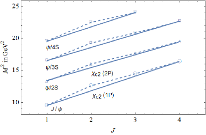
Figure 1: $(J,M^{2})$ Regge trajectory of parent and daughter for charmonium with un-natural parity. Solid shapes indicates predicted mass, hollow circle represent experimental masses

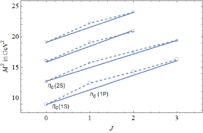
Figure 2: Regge trajectory $(J,M^{2})$ of $c\bar{c}$ meson with unnatural parity

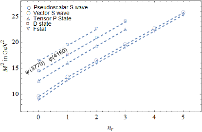
Figure 3: Regge trajectory $(n_{r},M^{2})$ for the Pseudoscaler and vector S state, excited P and D state masses of the $c\bar{c}$ meson

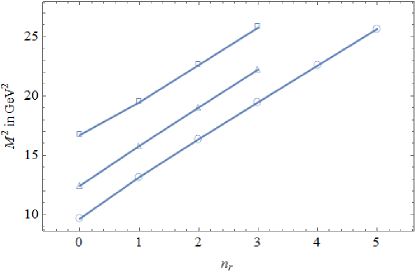
Figure 4: Regge trajectory $(n_{r},M^{2})$ for the S-P-D States center of weight mass for the $c\bar{c}$ meson

Table 14: Fitted parameters of the $(J,M^{2})$ Regge trajectory with natural and unnatural parity

Parity	$c\bar{c}$	$\alpha(GeV^{-2})$	$\alpha_{0}$
	Parent	0.439$\pm$0.038	-3.333$\pm$0.515
Natural	First Daughter	0.487$\pm$0.039	-5.598$\pm$0.650
	Second Daughter	0.491$\pm$0.046	-7.230$\pm$0.921
	Third Daughter	0.438$\pm$0.077	-7.660$\pm$1.739
	Parent	0.407$\pm$0.045	-3.786$\pm$0.062
Unnatural	First Daughter	0.446$\pm$0.042	-5.828$\pm$0.708
	Second Daughter	0.451$\pm$0.046	-7.355$\pm$0.910
	Third Daughter	0.398$\pm$0.063	-7.667$\pm$1.380

Table 15: Fitted parameters of Regge trajectory $(n_{r},M^{2})$ for the S-P-D states

$c\bar{c}$	JP̂	$\beta(GeV^{-2})$	$\beta_{0}$
S	$0^{-}$	0.308$\pm$0.006	-2.855$\pm$0.106
S	$1^{-}$	0.312$\pm$0.005	-3.082$\pm$0.103
P	$2^{+}$	0.303$\pm$0.003	-3.840$\pm$0.051
D	$1^{-}$	0.311$\pm$0.002	-4.458$\pm$0.031
D	$3^{-}$	0.321$\pm$0.000	-5.270$\pm$0.017

Table 16: Fitted parameters of Regge trajectory $(n_{r},M^{2})$ for the S-P-D states center of weight mass

$c\bar{c}$	$\beta(GeV^{-2})$	$\beta_{0}$
S	0.314$\pm$0.004	-3.102$\pm$0.068
P	0.306$\pm$0.002	-3.823$\pm$0.044
D	0.329$\pm$0.007	-5.470$\pm$0.160

6.1 Mass spectra

The mass difference between the S wave states, $1^{1}S_{0}$ - $1^{3}S_{1}$ is 105 MeV and $2^{1}S_{0}$ - $2^{3}S_{1}$ is 114 MeV for the present calculations, while in Chaturvedi:2018xrg the mass difference was 82 and 63 MeV respectively, experimentally observed mass difference is 113 and 47 MeV. Thus in the present calculation the splitting in S wave degenerate mesonic states has significantly increased for both 1S and 2S states, bringing the calculated masses nearby the experimental ones. For $3^{3}S_{1}$ and $4^{3}S_{1}$ states our calculated masses are only 30 MeV and 7 MeV greater than the experimentally observed masses, which is a considerably improved result as compared toChaturvedi:2018xrg and other theoretical studies tabulated. For 1P states it can be seen that the calculate masses of $1^{1}P_{1}$ , $1^{3}P_{0}$ , $1^{3}P_{1}$ and $1^{3}P_{2}$ when compared with experimentally observed masses differ only by 02, 59, 04 & 5 MeV respectively. Based on our calculation of mass spectrum we associate ${{\boldsymbol{\chi}}_{{c0}}{(3915)}}$ or ${{\mathit{X}}{(3915)}}$ as $2^{3}P_{0}$ state, both of them share same parity and there is no mass difference between our calculated and experimentally observed value. Also, we associate ${{\boldsymbol{\chi}}_{{c1}}{(3872)}}$Tanabashi:2018oca as $2^{3}P_{1}$ state because both of them share same parity and as shown in Fig.1 it lies on the curve which inspires us for this association and the mass difference between our calculated and experimental value is 78 MeV. For $2^{3}P_{2}$ state the mass difference between our calculated and experimental value is 75 MeV. There are no experimentally observed states for 5S, 6S, 3P and 4P hence we compare our results with theoretical results only and observe that our values are good consonance with the relativistic modelEbert:2011jc but suppressed when compared with Cornell potential approachChaturvedi:2018xrg ; Soni:2017wvy . There is only one experimentally observed state in D and beyond i.e. $1^{3}D_{2}$Bhardwaj:2013rmw and our calculated mass is less than experimental value by 22 MeV. We associate ${{\boldsymbol{\psi}}{(3770)}}$ as $1^{3}D_{1}$ state because both of them have same parity and the difference between our calculated and experimentally observed mass is 12 MeV which lies in the error bar. Also, we associate ${{\boldsymbol{\psi}}{(4160)}}$ as $2^{3}D_{1}$ state as both of them have same parity also the mass difference between our calculated and experimental value is only 05 MeV. In $(n_{r},M^{2})$ Regge trajectory both ${{\boldsymbol{\psi}}{(3770)}}$ and ${{\boldsymbol{\psi}}{(4160)}}$ lie on the curve and follow linearity and parallelism thus helping us to associate them with $1^{3}D_{1}$ and $2^{3}D_{1}$ charmonium states.

6.2 Decay Properties

Using the potential parameters and reduced normalized wave function we compute the various decay properties like $\gamma\gamma$, $e^{+}e^{-}$, light hadron and $\gamma\gamma\gamma$ decay widths of various states of charmonium, also the $E1$ & $M1$ transition widths have been calculated in present study. The ${}^{1}S_{0}\rightarrow\gamma\gamma$ decay width within the framework of NRQCD has been calculated by four different approaches, $i.e.$ at NNLO in $\nu$, at NLO in $\nu^{2}$, at $O(\alpha_{s}\nu^{2})$ and at NLO in $\nu^{4}$. The calculated results are tabulated in table 5 and is compared with experimentally observed decay widthsTanabashi:2018oca , relativistic quark model (RQM)Ebert:2002pp , heavy quark spin symmetryLansberg:2006dw , relativistic Salpeter modelKim:2004rz and the decay widths calculated by conventional Van Royen-Weisskopf formulaSoni:2017wvy ; Chaturvedi:2018xrg . The values of the decay widths calculated at NLO in $\nu^{4}$ is more convincing then the decay width obtained by the rest three approaches and is nearby the experimental results as well.
In addition the $n\chi_{0,2}\rightarrow\gamma\gamma$ decay width by NRQCD mechanism is also calculated at NLO in $\nu^{2}$ and at NNLO in $\nu^{2}$, the obtained results are tabulated in table 6 and compared with experimental and other theoretical decay widths. It is observed that the calculated decay width by both approaches are more or less same and nearby the experimental decay width.
The ${}^{3}S_{1}\rightarrow e^{+}e^{-}$ decay width within NRQCD framework has been calculated at NLO in $\nu$, NNLO in $\nu$, NLO in $\nu^{2}$, NLO in $\alpha_{s}\nu^{4}$ and NLO in $\alpha_{s}^{2}\nu^{4}$. The results obtained are tabulated in table 7 and are compared with experimental and other theoretical decay widths. It can be commented that the decay width obtained at NLO in $\alpha_{s}\nu^{4}$ is nearby the experimental decay width, as compared with the decay width calculated by other approach.
The ${}^{1}S_{0}\rightarrow LH$ decay width, at NLO in $\nu^{2}$ and at NNLO in $\nu^{2}$ has been calculated and the results are tabulated in table 8, it can be observed that the calculated decay width from both the current approaches has considerably improved as compared to the previous approachChaturvedi:2018xrg and is same as the experimentally determined decay width.
The ${}^{3}S_{1}\rightarrow\gamma\gamma\gamma$ decay width calculated at NLO $\nu^{2}$ is tabulated in table 9, the result is found to be in perfect agreement with PDG data Tanabashi:2018oca .
The results for $E1$ and $M1$ transition for charmonium have been listed in Tables 12 & 13. The obtained results are compared with experimental and other theoretical approaches like linear potential model, screened potential model, relativistic potential model and non-relativistic potential model. It is observed that for the transitions which are experimentally observed our calculated widths are in excellent agreement. Also for transition widths which are not observed experimentally our calculated values are comparable with values obtained by other theoretical approaches. Ratio of $\frac{\Gamma_{ee}(nS)}{\Gamma_{ee}(1S)}$ in Table 17 is consistent with experimental data.

Table 17: The ratios of $\frac{\Gamma_{e^{+}e^{-}}{{\mathit{J}/\psi}}(nS)}{\Gamma_{e^{+}e^{-}}{{\mathit{J}/\psi}{(1S)}}}$ for charmonium states

$\frac{\Gamma_{e^{+}e^{-}}{{\mathit{J}/\psi}}(nS)}{\Gamma_{e^{+}e^{-}}{{\mathit{J}/\psi}{(1S)}}}$	Present	Expt. Tanabashi:2018oca	Bhavsar:2018umj
$\frac{\Gamma_{e^{+}e^{-}}{{\mathit{J}/\psi}}(2S)}{\Gamma_{e^{+}e^{-}}{{\mathit{J}/\psi}{(1S)}}}$	0.295	0.43	0.39
$\frac{\Gamma_{e^{+}e^{-}}{{\mathit{J}/\psi}}(3S)}{\Gamma_{e^{+}e^{-}}{{\mathit{J}/\psi}{(1S)}}}$	0.124	–	0.21
$\frac{\Gamma_{e^{+}e^{-}}{{\mathit{J}/\psi}}(4S)}{\Gamma_{e^{+}e^{-}}{{\mathit{J}/\psi}{(1S)}}}$	0.067	–	0.11
$\frac{\Gamma_{e^{+}e^{-}}{{\mathit{J}/\psi}}(5S)}{\Gamma_{e^{+}e^{-}}{{\mathit{J}/\psi}{(1S)}}}$	0.042	–	0.04

6.3 Charmoniumlike states as admixtures

${{\boldsymbol{\psi}}{(4230)}}$, ${{\boldsymbol{\psi}}{(4260)}}$ & ${{\boldsymbol{\psi}}{(4360)}}$ all having J^P as $1^{-}$ and lie within $100$ MeV mass range, all three states can have properties different from conventional charmonia state, detailed literature about them has been discussed in introduction part of this article. Because they are so narrowly placed we explain all of them as admixtures of $3^{3}S_{1}$ and $3^{3}D_{1}$ charmonia states. As per our calculation all three admixture states have 41%, 36% & 51% contribution from S wave counterpart, our calculated masses of ${{\boldsymbol{\psi}}{(4230)}}$, ${{\boldsymbol{\psi}}{(4260)}}$ & ${{\boldsymbol{\psi}}{(4360)}}$ match well with their experimental mass. Except for ${{\boldsymbol{\psi}}{(4230)}}$ state, calculated masses of ${{\boldsymbol{\psi}}{(4260)}}$ & ${{\boldsymbol{\psi}}{(4360)}}$ lie within error bar suggested by PDGTanabashi:2018oca . Also, to strengthen our claim about these states as admixtures we calculate their leptonic decay widths and compare with experimentally observed result. We observe that our calculated leptonic decay width of ${{\boldsymbol{\psi}}{(4230)}}$ state when compared with BESIIIAblikim:2015dlj is approximately $8$ MeV greater, while leptonic decay widths of ${{\boldsymbol{\psi}}{(4260)}}$ & ${{\boldsymbol{\psi}}{(4360)}}$ when compared with PDGTanabashi:2018oca and BaBarLees:2014iua differs by $1.9$ and $4.4$ MeV respectively. Thus we comment that any of ${{\boldsymbol{\psi}}{(4230)}}$, ${{\boldsymbol{\psi}}{(4260)}}$ & ${{\boldsymbol{\psi}}{(4360)}}$ states can be admixture of $3^{3}S_{1}$ and $3^{3}D_{1}$ pure charmonia states.
Very less is known about ${{\boldsymbol{\psi}}{(4390)}}$ both theoretically and experimentally, we in present work try to study it as admixture of $3^{3}S_{1}$ and $3^{3}D_{1}$, our calculated mass differs from experimental mass by $60$ MeV. Experimental leptonic decay width has not been observed but we calculate it to be $2.11$ eV. Due to lack of experimental evidence and scarce theoretical study we are reluctant to mention it as an admixture state and hope that experiments in future can throw more light on this state.
${{\boldsymbol{\psi}}{(4660)}}$ has been studied as a molecular state and also as admixture state byBhavsar:2018umj . Having J^P as $1^{-}$ we associate it as admixture state of $4^{3}S_{1}$ and $4^{3}D_{1}$ having 43% contribution of $4^{3}S_{1}$. Our calculate mass is in perfect agreement with PDG mass, we have also calculated its leptonic decay width, which is approximately $3$ eV less than than decay width observed by BelleWang:2014hta . Based on our study we claim it to be an admixture of $4^{3}S_{1}$ and $4^{3}D_{1}$ pure charmonium states.

A detailed description of ${{\boldsymbol{\chi}}_{{c1}}{(4140)}}$ and ${{\boldsymbol{\chi}}_{{c1}}{(4274)}}$ both having J^P as $1^{+}$ has been discussed in introduction, they have been predicted as tetra-quark state or a hybrid state by some theorist, and ${{\boldsymbol{\chi}}_{{c1}}{(4140)}}$ has been predicted as a pure $3^{3}P_{0}$ state byBhavsar:2018umj . Based on our calculation we suggest ${{\boldsymbol{\chi}}_{{c1}}{(4140)}}$ as $3^{3}P_{1}$ and $2^{1}P_{1}$ admixture. And we suggest ${{\boldsymbol{\chi}}_{{c1}}{(4274)}}$ as $3^{3}P_{1}$ and $3^{1}P_{1}$ admixture. Our calculated mass is in agreement with experimental mass.

7 Conclusion

After looking at over all mass spectrum and various decay properties we comment that the potential employed here i.e. Cornell potential when coupled with relativistic correction in the framework of pNRQCD is successful in determining mass spectra and decay properties of charmonium. Thus helping us to support our choice of the potential in explaining quark anti-quark interaction in charmonium. Also, some experimental Charmoniumlike states as an admixture of nearby isoparity states have been explained. The constructed Regge trajectories are helpful for the association of some higher excited states to the family of Charmonium. But from our study we comment that more precise experimental studies is required to associate Charmoniumlike states as pure charmonium or as an exotic, molecular or some other states.

8 Appendix

1. Explanation of the symbols in Equations 3.1 & 21. $\psi$ & $\chi$ are Pauli spinor fields that creates heavy quark and anti-quark, $\overrightarrow{D}$ is gauge covariant spatial derivative, and $\psi^{{\dagger}}$ & $\chi^{{\dagger}}$ are mixed two fermion operator corresponding to the annihilation (or creation) of $Q\bar{Q}$ pair respectively.

2. Explanation of various symbols appearing in the short distance coefficients in Equations 3.1, 16, 17, 19, 3.2, 27, 28, 3.3 & 3.3; $Q$ is charge of the charm quark its value is $2/3$, $\alpha$ is electromagnetic running coupling constant its value is $1/137$, $C_{f}=(N_{c}^{2}-1)/2N_{c}$ is the Casimir for the fundamental representation, $\alpha_{s}$ is strong running coupling constant its value is given in table 2 and $n_{f}$ corresponds to the flavour of light quark.

3. In Equation 3.1 the terms are the operators responsible for $\gamma\gamma$ decay of $n^{1}S_{0}$ states, where (n=1 to 6). $\left|\left<0|\chi^{{\dagger}}\psi|^{1}S_{0}\right>\right|^{2}$, $\left[\left<{}^{1}S_{0}|\psi^{{\dagger}}\chi|0\right>\left<0|\chi^{{\dagger}}\left(-\frac{i}{2}\overrightarrow{D}\right)^{2}\psi|^{1}S_{0}\right>\right]$,
   $\left[\left<{}^{1}S_{0}|\psi^{{\dagger}}\left(-\frac{i}{2}\overrightarrow{D}\right)^{2}\chi|0\right>\left<0|\chi^{{\dagger}}\left(-\frac{i}{2}\overrightarrow{D}\right)^{2}\psi|^{1}S_{0}\right>\right]$ and $\left[\left<{}^{1}S_{0}|\psi^{{\dagger}}\chi|0\right>\left<0|\chi^{{\dagger}}\left(-\frac{i}{2}\overrightarrow{D}\right)^{4}\psi|^{1}S_{0}\right>\right]$.

4. In Equation 21 the terms are the operators responsible for $e^{+}e^{-}$ decay of $n^{3}S_{1}$ states states, where (n=1 to 6). $\left|\left<0|\chi^{{\dagger}}\psi|^{1}S_{0}\right>\right|^{2}$,
   $\left[\left<{}^{3}S_{1}|\psi^{{\dagger}}\sigma\chi|0\right>\left<0|\chi^{{\dagger}}\sigma\left(-\frac{i}{2}\overrightarrow{D}\right)^{2}\psi|^{3}S_{1}\right>\right]$,
   $\left[\left<0|\chi^{{\dagger}}\sigma\left(-\frac{i}{2}\overrightarrow{D}\right)^{2}\psi|^{3}S_{1}\right>\right]$ and
   $\left[\left<{}^{3}S_{1}|\psi^{{\dagger}}\sigma\chi|0\right>\left<0|\chi^{{\dagger}}\sigma\left(-\frac{i}{2}\overrightarrow{D}\right)^{4}\psi|^{3}S_{1}\right>\right]$.

5. The $F^{\prime}s,G^{\prime}s$ and $H^{\prime}s$ in Equations 3.1 & 21 are expressed in terms of various parameters in Equations 3.1 & 3.2.

6. In Equation 3.1 the operators are expressed in terms of matrix elements. $\left<{}^{1}S_{0}|{\cal{O}}(^{1}S_{0})|^{1}S_{0}\right>$, $\left<{}^{1}S_{0}|{\cal{P}}_{1}(^{1}S_{0})|^{1}S_{0}\right>$ and $\left<{}^{1}S_{0}|{\cal{Q}}^{1}_{1}(^{1}S_{0})|^{1}S_{0}\right>$ are the matrix elements for the decay of $n^{1}S_{0}$ states into $\gamma\gamma$. In Equation 3.2 the operators $\left<{}^{3}S_{1}|{\cal{O}}(^{3}S_{1})|^{3}S_{1}\right>$, $\left<{}^{3}S_{1}|{\cal{P}}_{1}(^{3}S_{1})|^{3}S_{1}\right>$ and
   $\left<{}^{3}S_{1}|{\cal{Q}}^{1}_{1}(^{3}S_{1})|^{3}S_{1}\right>$ are the matrix elements for the decay of $n^{3}S_{1}$ states into $e^{+}e^{-}$.

7. In Equations 3.1 & 3.2 the matrix elements are expressed in terms of independent non-perturbative regularized and renormalized wave functions at origin. $|R_{P}(0)|^{2}$ and $|R_{V}(0)|^{2}$ are the square of the pseudoscalar and vector states wave function.

8. We have computed $\nabla^{2}R$ term as per Khan:1995np

   $$\nabla^{2}R = -xR\frac{M}{2},r\rightarrow 0$$ (46)

   The binding energy, $x=M-(2m_{Q})$; $M$ is mass of respective mesoni state and $Q$ being charge of the charm quark, $C_{F}=\frac{4}{3}$ and $\alpha=\frac{1}{137}$.

References

- (1) C. McNeile, C.T.H. Davies, E. Follana, K. Hornbostel, G.P. Lepage, Phys. Rev. D86, 074503 (2012). DOI 10.1103/PhysRevD.86.074503
- (2) J. Gasser, H. Leutwyler, Annals Phys. 158, 142 (1984). DOI 10.1016/0003-4916(84)90242-2
- (3) M. Neubert, Phys. Rept. 245, 259 (1994). DOI 10.1016/0370-1573(94)90091-4
- (4) E.V. Veliev, K. Azizi, H. Sundu, N. Aksit, J. Phys. G39, 015002 (2012). DOI 10.1088/0954-3899/39/1/015002
- (5) G.T. Bodwin, E. Braaten, G.P. Lepage, Phys. Rev. D51, 1125 (1995). DOI 10.1103/PhysRevD.55.5853,10.1103/PhysRevD.51.1125. [Erratum: Phys. Rev.D55,5853(1997)]
- (6) C.H. Llewellyn-Smith, Annals Phys. 53, 521 (1969). DOI 10.1016/0003-4916(69)90035-9
- (7) A.N. Mitra, B.M. Sodermark, Nucl. Phys. A695, 328 (2001). DOI 10.1016/S0375-9474(01)01115-0
- (8) R. Ricken, M. Koll, D. Merten, B.C. Metsch, H.R. Petry, Eur. Phys. J. A9, 221 (2000). DOI 10.1007/s100500070041
- (9) A.N. Mitra, S. Bhatnagar, Int. J. Mod. Phys. A7, 121 (1992). DOI 10.1142/S0217751X92000077
- (10) P.C. Vinodkumar, J.N. Pandya, V.M. Bannur, S.B. Khadkikar, Eur. Phys. J. A4, 83 (1999). DOI 10.1007/s100500050206
- (11) J.N. Pandya, P.C. Vinodkumar, Pramana 57, 821 (2001). DOI 10.1007/s12043-001-0031-y
- (12) A. Kumar Rai, P.C. Vinodkumar, J.N. Pandya, J. Phys. G31, 1453 (2005). DOI 10.1088/0954-3899/31/12/007
- (13) A.K. Rai, J.N. Pandya, P.C. Vinodkumar, Indian J. Phys. A80, 387 (2006)
- (14) A.K. Rai, J.N. Pandya, P.C. Vinodkummar, Nucl. Phys. A782, 406 (2007). DOI 10.1016/j.nuclphysa.2006.10.023
- (15) J.N. Pandya, A.K. Rai, P.C. Vinodkumar, Frascati Phys. Ser. 46, 1519 (2007)
- (16) P.C. Vinodkumar, A.K. Rai, B. Patel, J. Pandya, Frascati Phys. Ser. 46, 929 (2007)
- (17) A.K. Rai, J.N. Pandya, P.C. Vinodkumar, Eur. Phys. J. A38, 77 (2008). DOI 10.1140/epja/i2008-10639-9
- (18) J.N. Pandya, N.R. Soni, N. Devlani, A.K. Rai, Chin. Phys. C39(12), 123101 (2015). DOI 10.1088/1674-1137/39/12/123101
- (19) N. Brambilla, et al., Eur. Phys. J. C71, 1534 (2011). DOI 10.1140/epjc/s10052-010-1534-9
- (20) S.K. Choi, et al., Phys. Rev. Lett. 91, 262001 (2003). DOI 10.1103/PhysRevLett.91.262001
- (21) D. Acosta, et al., Phys. Rev. Lett. 93, 072001 (2004). DOI 10.1103/PhysRevLett.93.072001
- (22) E. Braaten, L.P. He, K. Ingles, (2018)
- (23) Y.S. Kalashnikova, A.V. Nefediev, (2018). DOI 10.3367/UFNe.2018.08.038411
- (24) E.S. Swanson, Phys. Lett. B598, 197 (2004). DOI 10.1016/j.physletb.2004.07.059
- (25) C. Hanhart, Yu.S. Kalashnikova, A.E. Kudryavtsev, A.V. Nefediev, Phys. Rev. D76, 034007 (2007). DOI 10.1103/PhysRevD.76.034007
- (26) F. Aceti, R. Molina, E. Oset, Phys. Rev. D86, 113007 (2012). DOI 10.1103/PhysRevD.86.113007
- (27) J. Ferretti, G. Galatà, E. Santopinto, Phys. Rev. C88(1), 015207 (2013). DOI 10.1103/PhysRevC.88.015207
- (28) T. Barnes, S. Godfrey, E.S. Swanson, Phys. Rev. D72, 054026 (2005). DOI 10.1103/PhysRevD.72.054026
- (29) M.R. Pennington, D.J. Wilson, Phys. Rev. D76, 077502 (2007). DOI 10.1103/PhysRevD.76.077502
- (30) I.V. Danilkin, Yu.A. Simonov, Phys. Rev. Lett. 105, 102002 (2010). DOI 10.1103/PhysRevLett.105.102002
- (31) M. Karliner, J.L. Rosner, Phys. Rev. D91(1), 014014 (2015). DOI 10.1103/PhysRevD.91.014014
- (32) M. Cardoso, G. Rupp, E. van Beveren, Eur. Phys. J. C75(1), 26 (2015). DOI 10.1140/epjc/s10052-014-3254-z
- (33) A.M. Badalian, Yu.A. Simonov, B.L.G. Bakker, Phys. Rev. D91(5), 056001 (2015). DOI 10.1103/PhysRevD.91.056001
- (34) M. Tanabashi, et al., Phys. Rev. (3), 030001 (2018). DOI 10.1103/PhysRevD.98.030001
- (35) V. Kher, A.K. Rai, Chin. Phys. C42(8), 083101 (2018). DOI 10.1088/1674-1137/42/8/083101
- (36) A. Abulencia, et al., Phys. Rev. Lett. 98, 132002 (2007). DOI 10.1103/PhysRevLett.98.132002
- (37) T. Aaltonen, et al., Phys. Rev. Lett. 102, 242002 (2009). DOI 10.1103/PhysRevLett.102.242002
- (38) T. Aaltonen, et al., Mod. Phys. Lett. A32(26), 1750139 (2017). DOI 10.1142/S0217732317501395
- (39) V.M. Abazov, et al., Phys. Rev. D89(1), 012004 (2014). DOI 10.1103/PhysRevD.89.012004
- (40) S. Chatrchyan, et al., Phys. Lett. B734, 261 (2014). DOI 10.1016/j.physletb.2014.05.055
- (41) J. Brodzicka, Conf. Proc. C0908171, 299 (2009). DOI 10.3204/DESY-PROC-2010-04/38. [,299(2009)]
- (42) C.P. Shen, et al., Phys. Rev. Lett. 104, 112004 (2010). DOI 10.1103/PhysRevLett.104.112004
- (43) R. Aaij, et al., Phys. Rev. D85, 091103 (2012). DOI 10.1103/PhysRevD.85.091103
- (44) J.P. Lees, et al., Phys. Rev. D91(1), 012003 (2015). DOI 10.1103/PhysRevD.91.012003
- (45) X. Liu, S.L. Zhu, Phys. Rev. D80, 017502 (2009). DOI 10.1103/PhysRevD.85.019902,10.1103/PhysRevD.80.017502. [Erratum: Phys. Rev.D85,019902(2012)]
- (46) T. Branz, T. Gutsche, V.E. Lyubovitskij, Phys. Rev. D80, 054019 (2009). DOI 10.1103/PhysRevD.80.054019
- (47) R.M. Albuquerque, M.E. Bracco, M. Nielsen, Phys. Lett. B678, 186 (2009). DOI 10.1016/j.physletb.2009.06.022
- (48) G.J. Ding, Eur. Phys. J. C64, 297 (2009). DOI 10.1140/epjc/s10052-009-1146-4
- (49) F. Stancu, J. Phys. G37, 075017 (2010). DOI 10.1088/1361-6471/aaf026,10.1088/0954-3899/37/7/075017. [Erratum: J. Phys.G46,no.1,019501(2019)]
- (50) Z.g. Wang, Y.f. Tian, Int. J. Mod. Phys. A30, 1550004 (2015). DOI 10.1142/S0217751X15500049
- (51) V.V. Anisovich, M.A. Matveev, A.V. Sarantsev, A.N. Semenova, Int. J. Mod. Phys. A30(32), 1550186 (2015). DOI 10.1142/S0217751X15501869
- (52) Z.G. Wang, Eur. Phys. J. C63, 115 (2009). DOI 10.1140/epjc/s10052-009-1097-9
- (53) N. Mahajan, Phys. Lett. B679, 228 (2009). DOI 10.1016/j.physletb.2009.07.043
- (54) Q.F. Lü, Y.B. Dong, Phys. Rev. D94(7), 074007 (2016). DOI 10.1103/PhysRevD.94.074007
- (55) T. Bhavsar, M. Shah, P.C. Vinodkumar, Eur. Phys. J. C78(3), 227 (2018). DOI 10.1140/epjc/s10052-018-5694-3
- (56) S. Uehara, et al., Phys. Rev. Lett. 104, 092001 (2010). DOI 10.1103/PhysRevLett.104.092001
- (57) X. Liu, Z.G. Luo, Z.F. Sun, Phys. Rev. Lett. 104, 122001 (2010). DOI 10.1103/PhysRevLett.104.122001
- (58) J.P. Lees, et al., Phys. Rev. D86, 072002 (2012). DOI 10.1103/PhysRevD.86.072002
- (59) T. Branz, R. Molina, E. Oset, Phys. Rev. D83, 114015 (2011). DOI 10.1103/PhysRevD.83.114015
- (60) M. Ablikim, et al., Phys. Rev. Lett. 114(9), 092003 (2015). DOI 10.1103/PhysRevLett.114.092003
- (61) M. Ablikim, et al., Phys. Rev. Lett. 118(9), 092002 (2017). DOI 10.1103/PhysRevLett.118.092002
- (62) X.L. Wang, et al., Phys. Rev. Lett. 99, 142002 (2007). DOI 10.1103/PhysRevLett.99.142002
- (63) X.L. Wang, et al., Phys. Rev. D91, 112007 (2015). DOI 10.1103/PhysRevD.91.112007
- (64) J.P. Lees, et al., Phys. Rev. D89(11), 111103 (2014). DOI 10.1103/PhysRevD.89.111103
- (65) P.A. Rapidis, et al., Phys. Rev. Lett. 39, 526 (1977). DOI 10.1103/PhysRevLett.39.526,10.1103/PhysRevLett.39.974. [Erratum: Phys. Rev. Lett.39,974(1977)]
- (66) S. Godfrey, N. Isgur, Phys. Rev. D32, 189 (1985). DOI 10.1103/PhysRevD.32.189
- (67) R. Brandelik, et al., Phys. Lett. 76B, 361 (1978). DOI 10.1016/0370-2693(78)90807-9
- (68) X.L. Wang, Y.L. Han, C.Z. Yuan, C.P. Shen, P. Wang, Phys. Rev. D87(5), 051101 (2013). DOI 10.1103/PhysRevD.87.051101
- (69) X.L.e.a. Wang, Phys. Rev. D 87, 051101 (2013). DOI 10.1103/PhysRevD.87.051101. URL https://link.aps.org/doi/10.1103/PhysRevD.87.051101
- (70) B. Aubert, et al., Phys. Rev. Lett. 95, 142001 (2005). DOI 10.1103/PhysRevLett.95.142001
- (71) M. Cleven, Q. Wang, F.K. Guo, C. Hanhart, U.G. Meißner, Q. Zhao, Phys. Rev. D90(7), 074039 (2014). DOI 10.1103/PhysRevD.90.074039
- (72) O. Lakhina, E.S. Swanson, Phys. Rev. D74, 014012 (2006). DOI 10.1103/PhysRevD.74.014012
- (73) W.J. Deng, H. Liu, L.C. Gui, X.H. Zhong, Phys. Rev. D95(3), 034026 (2017). DOI 10.1103/PhysRevD.95.034026
- (74) W.J. Deng, H. Liu, L.C. Gui, X.H. Zhong, Phys. Rev. D95(7), 074002 (2017). DOI 10.1103/PhysRevD.95.074002
- (75) J. Segovia, P.G. Ortega, D.R. Entem, F. Fernández, Phys. Rev. D93(7), 074027 (2016). DOI 10.1103/PhysRevD.93.074027
- (76) S. Patel, P.C. Vinodkumar, S. Bhatnagar, Chin. Phys. C40(5), 053102 (2016). DOI 10.1088/1674-1137/40/5/053102
- (77) C. Bonati, M. D’Elia, A. Rucci, Phys. Rev. D92(5), 054014 (2015). DOI 10.1103/PhysRevD.92.054014
- (78) T. Gutsche, V.E. Lyubovitskij, I. Schmidt, A. Vega, Phys. Rev. D90(9), 096007 (2014). DOI 10.1103/PhysRevD.90.096007
- (79) M. Shah, A. Parmar, P.C. Vinodkumar, Phys. Rev. D86, 034015 (2012). DOI 10.1103/PhysRevD.86.034015
- (80) H. Negash, S. Bhatnagar, Int. J. Mod. Phys. E25(08), 1650059 (2016). DOI 10.1142/S0218301316500592
- (81) B.Q. Li, K.T. Chao, Phys. Rev. D79, 094004 (2009). DOI 10.1103/PhysRevD.79.094004
- (82) B.Q. Li, K.T. Chao, Commun. Theor. Phys. 52, 653 (2009). DOI 10.1088/0253-6102/52/4/20
- (83) C. Quigg, J.L. Rosner, Phys. Lett. 71B, 153 (1977). DOI 10.1016/0370-2693(77)90765-1
- (84) A. Martin, Phys. Lett. 93B, 338 (1980). DOI 10.1016/0370-2693(80)90527-4
- (85) W. Buchmuller, S.H.H. Tye, Phys. Rev. D24, 132 (1981). DOI 10.1103/PhysRevD.24.132
- (86) G.S. Bali, K. Schilling, C. Schlichter, Phys. Rev. D51, 5165 (1995). DOI 10.1103/PhysRevD.51.5165
- (87) G.S. Bali, B. Bolder, N. Eicker, T. Lippert, B. Orth, P. Ueberholz, K. Schilling, T. Struckmann, Phys. Rev. D62, 054503 (2000). DOI 10.1103/PhysRevD.62.054503
- (88) R. Chaturvedi, N.R. Soni, J.N. Pandya, A.K. Rai, (2018)
- (89) N. Brambilla, A. Pineda, J. Soto, A. Vairo, Rev. Mod. Phys. 77, 1423 (2005). DOI 10.1103/RevModPhys.77.1423
- (90) A. Pineda, J. Soto, Nucl. Phys. Proc. Suppl. 64, 428 (1998). DOI 10.1016/S0920-5632(97)01102-X. [,428(1997)]
- (91) N. Brambilla, A. Pineda, J. Soto, A. Vairo, Nucl. Phys. B566, 275 (2000). DOI 10.1016/S0550-3213(99)00693-8
- (92) P.G. Ortega, V. Mateu, D.R. Entem, F. Fernández, (2018)
- (93) Y..K. Koma, Few-Body Syst 54, 1027 (2013). DOI 10.1007/s00601-012-0542-8
- (94) W. Lucha, F.F. Schoberl, Int. J. Mod. Phys. C10, 607 (1999). DOI 10.1142/S0129183199000450
- (95) N. Brambilla, A. Pineda, J. Soto, A. Vairo, Phys. Rev. D63, 014023 (2001). DOI 10.1103/PhysRevD.63.014023
- (96) Y. Koma, M. Koma, Few-Body Systems 54 (2013). DOI 10.1007/s00601-012-0542-8
- (97) G. Perez-Nadal, J. Soto, Phys. Rev. D79, 114002 (2009). DOI 10.1103/PhysRevD.79.114002
- (98) Q. Huang, D.Y. Chen, X. Liu, T. Matsuki, Eur. Phys. J. C79(7), 613 (2019). DOI 10.1140/epjc/s10052-019-7121-9
- (99) R. Chaturvedi, A. Kumar Rai, Eur. Phys. J. Plus 133(6), 220 (2018). DOI 10.1140/epjp/i2018-12044-8
- (100) D. Ebert, R.N. Faustov, V.O. Galkin, Eur. Phys. J. C71, 1825 (2011). DOI 10.1140/epjc/s10052-011-1825-9
- (101) M.A. Sultan, N. Akbar, B. Masud, F. Akram, Phys. Rev. D90(5), 054001 (2014). DOI 10.1103/PhysRevD.90.054001
- (102) N.R. Soni, B.R. Joshi, R.P. Shah, H.R. Chauhan, J.N. Pandya, Eur. Phys. J. C78(7), 592 (2018). DOI 10.1140/epjc/s10052-018-6068-6
- (103) M. Kalinowski, M. Wagner, Phys. Rev. D92(9), 094508 (2015). DOI 10.1103/PhysRevD.92.094508
- (104) V. Bhardwaj, et al., Phys. Rev. Lett. 111(3), 032001 (2013). DOI 10.1103/PhysRevLett.111.032001
- (105) E. Braaten, S. Fleming, Phys. Rev. D52, 181 (1995). DOI 10.1103/PhysRevD.52.181
- (106) G.T. Bodwin, A. Petrelli, Phys. Rev. D66, 094011 (2002). DOI 10.1103/PhysRevD.87.039902,10.1103/PhysRevD.66.094011. [Erratum: Phys. Rev.D87,no.3,039902(2013)]
- (107) F. Feng, Y. Jia, W.L. Sang, Phys. Rev. Lett. 115(22), 222001 (2015). DOI 10.1103/PhysRevLett.115.222001
- (108) N. Brambilla, H.S. Chung, J. Komijani, Phys. Rev. D98(11), 114020 (2018). DOI 10.1103/PhysRevD.98.114020
- (109) Y. Jia, X.T. Yang, W.L. Sang, J. Xu, JHEP 06, 097 (2011). DOI 10.1007/JHEP06(2011)097
- (110) W.L. Sang, F. Feng, Y. Jia, S.R. Liang, Phys. Rev. D94(11), 111501 (2016). DOI 10.1103/PhysRevD.94.111501
- (111) D. Ebert, R.N. Faustov, V.O. Galkin, Phys. Rev. D67, 014027 (2003). DOI 10.1103/PhysRevD.67.014027
- (112) J.P. Lansberg, T.N. Pham, Phys. Rev. D74, 034001 (2006). DOI 10.1103/PhysRevD.74.034001
- (113) C.S. Kim, T. Lee, G.L. Wang, Phys. Lett. B606, 323 (2005). DOI 10.1016/j.physletb.2004.11.084
- (114) C. Amsler, et al., Phys. Lett. B667, 1 (2008). DOI 10.1016/j.physletb.2008.07.018
- (115) C.W. Hwang, R.S. Guo, Phys. Rev. D82, 034021 (2010). DOI 10.1103/PhysRevD.82.034021
- (116) S.N. Gupta, J.M. Johnson, W.W. Repko, Phys. Rev. D54, 2075 (1996). DOI 10.1103/PhysRevD.54.2075
- (117) H.W. Huang, K.T. Chao, Phys. Rev. D54, 6850 (1996). DOI 10.1103/PhysRevD.56.1821,10.1103/PhysRevD.54.6850. [Erratum: Phys. Rev.D56,1821(1997)]
- (118) P. Marquard, J.H. Piclum, D. Seidel, M. Steinhauser, Phys. Rev. D89(3), 034027 (2014). DOI 10.1103/PhysRevD.89.034027
- (119) W.M. Yao, et al., J. Phys. G33, 1 (2006). DOI 10.1088/0954-3899/33/1/001
- (120) F. Feng, Y. Jia, W.L. Sang, Phys. Rev. Lett. 119(25), 252001 (2017). DOI 10.1103/PhysRevLett.119.252001
- (121) N. Fabiano, G. Pancheri, Eur. Phys. J. C25, 421 (2002). DOI 10.1007/s10052-002-0974-2
- (122) P.B. Mackenzie, G.P. Lepage, Phys. Rev. Lett. 47, 1244 (1981). DOI 10.1103/PhysRevLett.47.1244
- (123) C. Patrignani, et al., Chin. Phys. C40(10), 100001 (2016). DOI 10.1088/1674-1137/40/10/100001
- (124) A.M. Badalian, B.L.G. Bakker, I.V. Danilkin, Phys. Atom. Nucl. 73, 138 (2010). DOI 10.1134/S1063778810010163
- (125) S.F. Radford, W.W. Repko, Nucl. Phys. A865, 69 (2011). DOI 10.1016/j.nuclphysa.2011.06.032
- (126) M. Shah, B. Patel, P.C. Vinodkumar, Eur. Phys. J. C76(1), 36 (2016). DOI 10.1140/epjc/s10052-016-3875-5
- (127) B.H. Yazarloo, H. Mehraban, EPL 115(2), 21002 (2016). DOI 10.1209/0295-5075/115/21002
- (128) M. Ablikim, et al., Phys. Rev. Lett. 115(1), 011803 (2015). DOI 10.1103/PhysRevLett.115.011803
- (129) J.P. Lees, et al., Phys. Rev. D89(11), 112004 (2014). DOI 10.1103/PhysRevD.89.112004
- (130) E. Eichten, K. Gottfried, T. Kinoshita, J.B. Kogut, K.D. Lane, T.M. Yan, Phys. Rev. Lett. 34, 369 (1975). DOI 10.1103/PhysRevLett.34.369,10.1103/PhysRevLett.36.1276. [Erratum: Phys. Rev. Lett.36,1276(1976)]
- (131) E. Eichten, K. Gottfried, T. Kinoshita, K.D. Lane, T.M. Yan, Phys. Rev. D17, 3090 (1978). DOI 10.1103/PhysRevD.17.3090,10.1103/physrevd.21.313.2. [Erratum: Phys. Rev.D21,313(1980)]
- (132) L. Cao, Y.C. Yang, H. Chen, Few Body Syst. 53, 327 (2012). DOI 10.1007/s00601-012-0478-z
- (133) H. Khan, P. Hoodbhoy, Phys. Rev. D53, 2534 (1996). DOI 10.1103/PhysRevD.53.2534