Regularised Atomic Body-Ordered Permutation-Invariant Polynomials
for the Construction of Interatomic Potentials

Abstract

We investigate the use of invariant polynomials in the construction of data-driven interatomic potentials for material systems. The “atomic body-ordered permutation-invariant polynomials” (aPIPs) comprise a systematic basis and are constructed to preserve the symmetry of the potential energy function with respect to rotations and permutations. In contrast to kernel based and artificial neural network models, the explicit decomposition of the total energy as a sum of atomic body-ordered terms allows to keep the dimensionality of the fit reasonably low, up to just 10 for the 5-body terms. The explainability of the potential is aided by this decomposition, as the low body-order components can be studied and interpreted independently. Moreover, although polynomial basis functions are thought to extrapolate poorly, we show that the low dimensionality combined with careful regularisation actually leads to better transferability than the high dimensional, kernel based Gaussian Approximation Potential.

I Introduction

There is a long and successful history of using empirical interatomic potentials for the simulation of materials Finnis (2004). One approach is to treat such models as purely phenomenological, setting out a few key features of the true interaction to be captured (e.g. the stability ordering of certain phases), and investigate what other properties, both macroscopic or indeed microscopic, follow from these. More recently, as electronic structure calculations, particularly density functional theory (DFT) Parr (1980), has increased both in accuracy and availability, there has been a widely shared desire for potentials to match the Born-Oppenheimer potential energy surface as closely as possible Ercolessi and Adams (1994); Murrell (1984). This change of attitude in the materials simulation community has come rather later than the analogous one in the world of organic force fields, partly due to the more systematic nature of quantum chemistry methods applicable to small molecules Atkins and Friedman (2011); Huang et al. (2005).

Already a decade ago, it was clear that empirical potentials had reached their limits in terms of their ability to match the potential energy surface of DFT, essentially due to the use of simple, physically interpretable functional forms. At around the same time significant developments started in which models with thousands of free parameters (so-called high-dimensional models) were fitted to electronic structure data. The methods are borrowed from machine learning, e.g. artificial neural networks (ANN) Jain et al. (1996); Bishop (2006); Behler and Parrinello (2007) and Gaussian processes (GP) Rasmussen and Williams (2005); Bartók and Csányi (2015). Although formally these models contain many degrees of freedom, they are often called non-parametric, because there are either good recipes for determining the best parameters that fit the data (in the case of training ANNs), or linear algebra expressions in the case of GPs. The few model parameters that are still adjusted by hand or by other ad-hoc recipes are called hyper-parameters, e.g. the nonlinear transfer function of ANN units, or the kernel shapes in GPs. It was understood early on, similarly to the more traditional applications of machine learning, that it is advantageous to use an appropriate representation of the input data (atomic positions in this case) that captures all the known symmetries present in the problem Bartók et al. (2013). These models achieve very high accuracy on the training datasets and, when carefully used, on configurations that are “near” the training, e.g., in a molecular dynamics run under similar conditions. However, the transferability of such models can still be poor. A recent attempt at assembling and fitting to a very large and diverse training dataset of elemental silicon Bartók et al. (2018), while generally staying physically sensible away from the training data, still showed up to 20% error in formation energies and migration barriers of some defects that were not in the training set. The data requirements to achieve even this level of transferability are expected to grow significantly for multicomponent systems.

While a better choice of representations and kernel functions may improve the transferability somewhat, it is conceivable that high-dimensional fits will, by their very nature, always suffer from this problem.

Similar effects can be seen in a related field, the fitting of the potential energy surfaces of molecules to high level, wave function based quantum chemistry calculations. This endeavour has a rich history Partridge and Schwenke (1997); Bramley and Carrington Jr. (1993); Cencek et al. (2008); Xie et al. (2005); Babin et al. (2013); Qu et al. (2018), which also includes high-dimensional nonparametric fits that are very accurate for small systems (a handful of atoms), yet it is recognised that once the dimensionality reaches a few tens, the fitting task becomes extremely difficult.

At present, the only plausible way to break the curse of dimensionality is to explicitly or implicitly identify low-dimensional structures of the potential energy surface. If this can be done explicitly then the energy can be broken up into multiple low-dimensional terms, ideally ensuring that higher dimensional terms account for less variation. The challenge is to do this generally, systematically, and without sacrificing accuracy.

A time-tested and obvious way to introduce low dimensional terms is to use the body order expansion applied in an atom-by-atom fashion Griebel (2006); Rabitz and Aliş (1999); Stillinger and Weber (1985); Nguyen et al. (2018); Glielmo et al. (2018); Sharma et al. (2006), i.e. define the total energy as a sum of one-atom, two-atom (pair), three-atom (angle) terms, and so forth. Let ${\mathbf{R}}\equiv\{{\mathbf{r}}_{j}\}_{j=1}^{M}$ be the positions of $M$ atomic nuclei of the same species, representing a configuration of atoms (perhaps but not necessarily with periodic boundary conditions), then we write the total energy as

$$E({\mathbf{R}}) =\sum_{j}E_{1}({\mathbf{r}}_{j})$$

$$\qquad+\frac{1}{2}\sum_{i\neq j}E_{2}({\mathbf{r}}_{i},{\mathbf{r}}_{j})$$

$$\qquad+\frac{1}{3!}\sum_{i\neq j\neq k}E_{3}({\mathbf{r}}_{i},{\mathbf{r}}_{j},{\mathbf{r}}_{k})$$ (1)

$$\qquad+\cdots+$$

$$\qquad+\frac{1}{N!}\sum_{i_{1}\neq\dots\neq i_{N}}E_{N}\big{(}{\mathbf{r}}_{i_{1}},\dots,{\mathbf{r}}_{i_{N}}).$$

Note that if the $n$-body function $E_{n}$ is permutation invariant then $\frac{1}{n!}\sum_{i_{1}\neq\dots\neq i_{n}}$ may of course be rewritten as $\sum_{i_{1}<\dots<i_{n}}$. Periodic boundary conditions are treated by taking into account the periodic images of atoms within the computational cell in (1).

We must strongly emphasize the distinction, on the one hand, between such a decomposition of the total energy into additive components, each of which only depends on few coordinates, and on the other hand the construction of complete, many-body, invariant representations of ${\mathbf{R}}$ using various combinations of two- and three-body functions, which are subsequently used in a single high-dimensional nonlinear nonparametric fit Rupp et al. (2012); Huo and Rupp (2017); Behler (2017). For example, consider the symmetry functions of Behler and Parrinello Behler (2011). Although each element of the descriptor is itself built out of just interatomic distances (2-body) or angles (3-body), the entire descriptor vector taken as a whole is a high dimensional description of the neighbour environment of an atom, and subsequent fits are of functions in that high dimensional space. In contrast, the individual energy terms in (1) are all low dimensional, and it is to be expected that they can be fitted using much less data, since low dimensional spaces can be covered comprehensively by a relatively small number of training configurations. In particular we conjecture excellent extrapolation properties. Note that this does not require an a priori definition or calculation of these terms, the fitting is still to be made to total energy $E$ and its derivatives (forces and stresses) corresponding to configurations with many atoms.

The utility of additive body order expansions has been recognised in the context of the recent machine learning based potentials. By writing the total energy as a sum of pair, triplet and a many-body terms with explicit weight factors Bartók and Csányi (2015); Deringer and Csányi (2017); Bartók et al. (2018), it is possible to prevent catastrophically erroneous predictions at small interatomic distances. Note that the failure of high dimensional fits at small interatomic distances is well known by the quantum chemists who fit small molecule potential energy surfaces Nandi et al. (2019).

However, merely writing the total energy as a body order expansion does not in itself bring the benefits of low dimensionality. The terms in (1) may be highly redundant, e.g. a general three-body potential includes all possible two-body potentials by simply not depending on one of its arguments, and this is true for all orders. A potential fitting methodology whose terms are intrinsically body-ordered was introduced as the Moment Tensor Potentials (MTPs) Shapeev (2016a), although it would appear that no explicit use is made of the lowest dimensional terms to maximise transferability. Recently, the Atomic Cluster Expansion (ACE) was introduced and the connection between the body order expansion and the high dimensional representations used in the earlier many-body fits was also made formally explicit Drautz (2019). There, transferability is achieved by defining and calculating the low order terms in (1) explicitly using the total energy function of small clusters: the order $M$ term is the interaction energy of the $M$-atom cluster in vacuum (with lower order interactions subtracted).

In both the MTP and the ACE approaches, a basis of symmetric polynomials is introduced, whose elements are body-ordered, and a linear fit in this basis is the fundamental modelling tool. The high computational cost of the many-body expansion is avoided by taking the entire many-body environment of each atom as a spatial density, and projecting it onto a rotationally invariant basis set, the components of which turn out to be body-ordered. This density trick is the same that is used by high-dimensional descriptors, including SOAP-GAP Bartók et al. (2013), Behler-Parrinello symmetry functions Behler (2011), and the bispectrum Bartók et al. (2010); Thompson et al. (2015), but without taking advantage of the body-ordered decomposition.

Finally, it is notable that yet another route to the atomic body ordered expansion is afforded by the Generalised Pseudopotential Theory approach of Moriarty Moriarty (1977, 1982, 1988). GPT treats perturbations of the electron density within the framework of density functional theory using the uniform electron gas as reference, and via a series of approximations derives individual body ordered terms formally - but also including the unit cell volume as a variable. It has had considerable success in modelling single species defect-free metals in an essentially parameter-free manner. Its extension to more complex materials is not straightforward, and calculating high body order terms (3- and 4-body terms) is rather complicated even for the simpler cases. Nevertheless GPT can be thought of as the explanation (or justification) of why the body order expansion is a good idea for strongly bound condensed phase materials, especially metals.

In this work, we will consider each body ordered term as an independent function to be fitted, but only whose sum is known. We will define a basis set with which we do a linear fit, so at the end, all the unknown basis coefficients may be determined in a single linear least squares problem, but separate and distinct distance based cutoffs and regularisation strategies are applied to each term. We will also forgo the vacuum-cluster definition of each term, and instead fit the basis coefficients directly to condensed phase data only. The advantage in fitting the body-order expansion to a condensed phase training set is that it can be expected to converge faster. Indeed, there is significant empirical evidence for this, such as the relative success of few-body interatomic potentials, cluster expansion for alloys Nelson et al. (2013), GPT Moriarty (1977, 1982, 1988), however, we are not aware of any rigorous results that explicitly show this in general.

For defining a basis set for the body ordered terms, we employ the theory of permutationally invariant polynomials (PIP) a technique based on classical invariant theory, introduced to molecular modelling for fitting the potential energy surfaces of small molecules; see e.g. Braams and Bowman (2009); Babin et al. (2013); Nguyen et al. (2018) and references therein. To adapt this formalism for condensed phase covalent materials we make two modifications: (i) an explicit introduction of distance-based cutoffs into the basis functions, and (ii) each body-ordered term has its own set of PIPs, taking account of the specific symmetry group of that term. By contrast, in the original application of PIPs to small molecules, each molecule (or a set of small molecules taken as a cluster) had its potential energy surface defined and fit with the appropriate set of PIPs and each new molecule or molecular cluster required a completely new fit. In a somewhat similar vein to our ideas here, the possibility to apply PIPs to manually determined subsets (fragments) of a molecule has previously been suggested in Braams and Bowman (2009) and very recently first explored in Qu and Bowman (2019).

We will call our basis set “atomic PIPs” or aPIPs, to emphasize that the body order expansion inherent to the use of PIPs is done here on an atomic rather than molecular basis. For the sake of simplicity, we limit the exposition here to elemental materials, but the formalism generalises naturally to multiple species, exactly in the same way as the original PIP formalism does for molecules.

Our overarching goal, for which the aPIP fits serve as examples, is to demonstrate for the case of materials (rather than isolated molecules) that (i) low body order potentials can reach the same high accuracies that high dimensional fits can, and (ii) polynomial fits can be used to improve generalisation properties of interatomic potentials and that sophisticated regularisation is the key to achieving this.

II Symmetric Polynomial Basis

Our starting assumption is that (1) can be used to construct high-accuracy PESs for moderate to low body-order $N$, which is certainly the case empirically. Next, we require that the individual contributions $E_{n}$ inherit rotation and permutation invariance (RPI) from $E$. Our aim is then to construct systematically improvable functional forms to represent individual $E_{n}$ functions that exactly preserve these symmetries:

1. Construct coordinate systems

   $$\mathbf{x}_{n}=\mathbf{x}_{n}({\mathbf{r}}_{1},\dots,{\mathbf{r}}_{n})$$

   that are continuous, rotation and permutation invariant, and represent

   $$E_{n}(\{{\mathbf{r}}_{i}\}_{i=1}^{n})=\Phi_{n}(\mathbf{x}_{n}(\{{\mathbf{r}}_{i}\})).$$

2. Choose basis sets $\{B_{nj}\}$ and represent

   $$\Phi_{n}(\mathbf{x})=\sum_{j}c_{nj}B_{nj}(\mathbf{x}).$$

3. Apply a cut-off mechanism to prevent inclusion of clusters with atoms that are very far from each other that have negligible contributions to the total energy.

4. Use regularised linear least squares (i.e., ridge regression, force matching Ercolessi and Adams (1994)) to determine the coefficients $\{c_{nj}\}_{n,j}$, using total energies, forces and stresses calculated by a first principles electronic structure approach as training data.

Several aspects of this strategy are familiar from recent machine-learning models: For example, the motivation for employing a RPI coordinate system is the same as for the use of symmetry functions descriptors for ANN potentials of Behler and Parrinello (2007) as well as the SOAP descriptor and kernel of the GAP framework of Bartók and Csányi (2015). Employing a polynomial basis to obtain a systematically improvable functional form was also proposed by Braams and Bowman (2009); Shapeev (2016b). We will import much of the invariant theory methodology for the representation of symmetric polynomials from Braams and Bowman (2009). In the following we will show how this approach leads to a large design space and in particular describe different coordinate systems as well as the basis functions to represent the potential energy.

II.1 Distance-based potentials

Our first construction of a RPI coordinate system is achieved by closely following the ideas of Braams and Bowman (2009): we first choose rotation invariant (${\rm RI}$) coordinates of transformed interatomic distances,

$$E_{n}(\{{\mathbf{r}}_{i}\}_{i=1}^{n})=E_{n}^{\rm D}(\{u_{ij}\}_{i<j=1}^{n}),$$

where $u_{ij}$ denotes a distance transform such as euclidean distance itself or the common Morse or inverse distance variables,

$$u_{ij}=r_{ij},\quad u_{ij}=e^{-\alpha r_{ij}},\quad u_{ij}=r_{ij}^{-p},$$

where $\alpha,p>0$. The superscript “D” in $E_{n}^{\rm D}$ indicates that the arguments of the function are distances. Alternatively, distances and angles can be used, which we discuss below and will denote with the superscript “DA”.

In the case of the 2-body term, $u_{12}$ is already a RPI coordinate system. For the 3-body contribution, the permutation invariance of $E_{3}$ with respect to exchanging atom indices gives rise to full $S_{3}$ permutation invariance of $E_{3}^{\rm D}$. Here, and throughout, $S_{n}$ denotes the symmetric group over $n$ elements. The elementary symmetric polynomials therefore give a permutation invariant coordinate system,

$$E_{3}({\mathbf{r}}_{1},{\mathbf{r}}_{2},{\mathbf{r}}_{3}) =E_{3}^{\rm D}(u_{12},u_{13},u_{23})$$

$$=\Phi_{3}^{\rm D}(f_{3,1},f_{3,2},f_{3,3}),$$

where

$$f_{3,1} =u_{12}+u_{13}+u_{23},$$

$$f_{3,2} =u_{12}u_{13}+u_{12}u_{23}+u_{13}u_{23},$$

$$f_{3,3} =u_{12}u_{13}u_{23}.$$ (2)

The key property of the coordinates $f_{3}=(f_{3,1},f_{3,2},f_{3,3})$ is that they completely define $({\mathbf{r}}_{1},{\mathbf{r}}_{2},{\mathbf{r}}_{3})$ up to rotations and permutations. The choice of such invariant coordinates is not unique. For example, we may choose $f_{n}=\sum_{i<j}u_{ij}^{n},n=1,2,3$ and in § II.2 we replace distance coordinates with distance and angle coordinates.

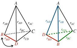
Figure 1: Permutation of the edges of a tetrahedron when two corners are permuted. In blue and green are permuted edges. Although there are six edges, the symmetry group of the edges induced by permuting pairs of atoms is a strict subset of $S_{6}$, which we denote by $S_{4}^{\rm D}$.

For the $n$-body terms with $n\geq 4$, the permutation group $S_{n}$ acting on $\{{\mathbf{r}}_{i}\}_{i=1}^{n}$ which encodes the symmetry of $E_{n}$ induces a non-trivial permutation group $S_{n}^{\rm D}\subsetneq S_{n(n-1)/2}$ acting on $\{u_{ij}\}_{i<j=1}^{n}$ encoding the symmetry of $E_{n}^{\rm D}$. That is, a permutation $\pi\in S_{n}$ of sites $\{{\mathbf{r}}_{i}\}$ is re-interpreted as a permutation in $S_{n}^{\rm D}$ of distances through the action

$$u_{ij}\overset{\pi}{\mapsto}u_{\pi i\pi j}$$

see Figure 1 for a visualisation in the four-body case.

Employing invariant theory techniques Derksen and Kemper (2015); Braams and Bowman (2009) we then construct fundamental invariants $f_{n}=\{f_{n,a}\}_{a=1}^{A_{n}}$, where $A_{n}>n$ is the dimensionality of the set $f_{n}$ and each $f_{n,a}$ is a multi-variate polynomial in $\{u_{ij}\}$ that is invariant under $S_{n}^{\rm D}$, such that we can rewrite $E_{n}$ as

$$E_{n}(\{{\mathbf{r}}_{i}\}_{i=1}^{n})=E_{n}^{\rm D}(\{u_{ij}\})=\Phi_{n}^{\rm D}(\{f_{n,a}\}).$$

A subtle point is that admissible arguments $\{u_{ij}\}$ and $\{f_{n,a}\}$ belong to $(3n-6)$-dimensional submanifolds of, respectively, ${\mathbb{R}}^{n(n-1)/2}$ and ${\mathbb{R}}^{A_{n}}$, where $n(n-1)/2>(3n-6)$ for $n\geq 5$ and $A_{n}>n(n-1)/2$ for $n\geq 4$; cf. Table 1. For illustration, a possible choice of the fundamental invariants for a 4-body distance-based potential are given in Table 2.

$n$	2	3	4	5	6
#coordinates	1	3	6	9	12
dim $\{u_{ij}\}$	1	3	6	10	15
$A_{n}$ = dim $\{f_{n,a}\}$	1	3	9	56	-

Table 1: Comparison of potential minimal number of coordinates, number of RI coordinates (distances), and number of RPI coordinates (fundamental invariants). For six-body invariants Magma terminated without computing the fundamental invariants within several weeks of CPU time. This is related to the rapidly increasing cardinality of the symmetry group (6! = 720). Note that restricting the polynomial degree shortens the computations, hence allows to compute invariants for higher body-orders, as is performed in Qu et al. (2013).

$f_{4,1}=$	$u_{12}+u_{13}+u_{14}+u_{23}+u_{24}+u_{34}$
$f_{4,2}=$	$u_{12}^{2}+u_{13}^{2}+u_{14}^{2}+u_{23}^{2}+u_{24}^{2}+u_{34}^{2}$
$f_{4,3}=$	$u_{12}u_{13}+u_{12}u_{14}+u_{12}u_{24}+u_{12}u_{34}$
	$+u_{13}u_{14}+u_{13}u_{23}+u_{13}u_{34}+u_{14}u_{23}$
	$+u_{14}u_{24}+u_{23}u_{24}+u_{23}u_{34}+u_{24}u_{34}$
$f_{4,4}=$	$u_{12}^{3}+u_{13}^{3}+u_{14}^{3}+u_{23}^{3}+u_{24}^{3}+u_{34}^{3}$
$f_{4,5}=$	$u_{12}u_{13}u_{14}+u_{12}u_{24}u_{34}+u_{13}u_{23}u_{34}+u_{14}u_{23}u_{24}$
$f_{4,6}=$	$u_{12}^{4}+u_{13}^{4}+u_{14}^{4}+u_{23}^{4}+u_{24}^{4}+u_{34}^{4}$
$f_{4,7}=$	$u_{12}^{2}u_{13}+u_{12}^{2}u_{14}+u_{12}^{2}u_{24}+u_{12}^{2}u_{34}+u_{12}u_{13}^{2}$
	$+u_{12}u_{14}^{2}+u_{12}u_{24}^{2}+u_{12}u_{34}^{2}+u_{13}^{2}u_{14}+u_{13}^{2}u_{23}$
	$+u_{13}^{2}u_{34}+u_{13}u_{14}^{2}+u_{13}u_{23}^{2}+u_{13}u_{34}^{2}+u_{14}^{2}u_{23}$
	$+u_{14}^{2}u_{24}+u_{14}u_{23}^{2}+u_{14}u_{24}^{2}+u_{23}^{2}u_{24}+u_{23}^{2}u_{34}$
	$+u_{23}u_{24}^{2}+u_{23}u_{34}^{2}+u_{24}^{2}u_{34}+u_{24}u_{34}^{2}$
$f_{4,8}=$	$u_{12}^{2}u_{13}u_{23}+u_{12}^{2}u_{14}u_{23}+u_{12}^{2}u_{23}u_{24}+u_{12}^{2}u_{23}u_{34}$
	$+u_{12}u_{13}^{2}u_{24}+u_{12}u_{13}u_{23}^{2}+u_{12}u_{13}u_{24}^{2}+u_{12}u_{14}^{2}u_{34}$
	$+u_{12}u_{14}u_{23}^{2}+u_{12}u_{14}u_{34}^{2}+u_{12}u_{23}^{2}u_{24}+u_{12}u_{23}^{2}u_{34}$
	$+u_{13}^{2}u_{14}u_{24}+u_{13}^{2}u_{23}u_{24}+u_{13}^{2}u_{24}u_{34}+u_{13}u_{14}^{2}u_{34}$
	$+u_{13}u_{14}u_{24}^{2}+u_{13}u_{14}u_{34}^{2}+u_{13}u_{23}u_{24}^{2}+u_{13}u_{24}^{2}u_{34}$
	$+u_{14}^{2}u_{23}u_{34}+u_{14}^{2}u_{24}u_{34}+u_{14}u_{23}u_{34}^{2}+u_{14}u_{24}u_{34}^{2}$
$f_{4,9}=$	$u_{12}^{2}u_{13}u_{23}^{2}+u_{12}^{2}u_{14}u_{23}^{2}+u_{12}^{2}u_{23}^{2}u_{24}+u_{12}^{2}u_{23}^{2}u_{34}$
	$+u_{12}u_{13}^{2}u_{24}^{2}+u_{12}u_{14}^{2}u_{34}^{2}+u_{13}^{2}u_{14}u_{24}^{2}+u_{13}^{2}u_{23}u_{24}^{2}$
	$+u_{13}^{2}u_{24}^{2}u_{34}+u_{13}u_{14}^{2}u_{34}^{2}+u_{14}^{2}u_{23}u_{34}^{2}+u_{14}^{2}u_{24}r_{34}^{2}.$

Table 2: 4B Distance-based invariants.

To complete the definition of $n$-body distance-based potentials, we supply $E_{n}$ with a cut-off mechanism, redefining them as

$$E_{n}(\{{\mathbf{r}}_{i}\}_{i=1}^{n})=\Phi_{n}^{\rm D}(f_{n})\prod_{i<j}f_{\rm cut}(r_{ij}),$$ (3)

where $f_{\rm cut}(r)$ is smooth and vanishes outside some cut-off radius $r_{\rm cut}$. That is, we only account for $n$-body clusters for which all edge lengths are within the cut-off radius. The choice of cut-off mechanism is far from unique of course, and can be adapted to the systems of interest.

II.2 Distance-angle potentials

While distance-based coordinates are seemingly canonical in that they inherit the maximum symmetry, it is sometimes intuitive to employ a coordinate system that incorporates more “physically natural” coordinates, which may lead to alternative ${\rm RI}$ and ${\rm RPI}$ coordinate systems. For example, the success of employing bond-angle coordinates in empirical force fields Stillinger and Weber (1985) suggests that using these coordinates may produce better fits at similar cost. This idea is further supported by the success of Moment Tensor Potentials Shapeev (2016b), which can be also interpreted as distance-angle potentials. Within our framework, many-body distance-angle potentials are constructed as follows.

As in § II.1 let $u_{ij}$ denote transformed distance coordinates. In addition, let $w_{ijk}$ denote angle coordinates, the canonical choice being

$$w_{ijk}=\cos\theta_{ijk}=\hat{{\mathbf{r}}}_{ij}\cdot\hat{{\mathbf{r}}}_{ik},$$

where ${\mathbf{r}}_{ij}={\mathbf{r}}_{j}-{\mathbf{r}}_{i}$ and $\hat{{\mathbf{r}}}={\mathbf{r}}/|{\mathbf{r}}|$. We then write an $n$-body term $E_{n}$ in a way that retains only partial symmetry,

$$E_{n}(\{{\mathbf{r}}_{i}\}_{i=1}^{n})=E_{n}^{\rm DA}(\{u_{1j}\}_{j=2}^{n},\{w_{1jk}\}_{j<k=2}^{n}\big{)},$$

where the superscript “DA” indicates that the function $E_{n}^{\rm DA}$ is parametrised by distances and angles. The 2-body contribution $E_{2}$ is again a pure distance-based potential.

For body order $n\geq 3$, we transform again to an RPI coordinate system. For the distance-angle potentials we retain only permutation invariance with respect to the $n-1$ neighbours, which induces a different symmetry group $S_{n-1}^{\rm DA}$ on the coordinates $(\{u_{1j}\}_{j},\{w_{1jk}\}_{jk})$. Analogously to the distance based potentials, the fundamental polynomial invariants for this permutation group $S_{n-1}^{\rm DA}$ yield a RPI coordinate system $f_{n}=f_{n}(\{u_{1j}\}_{j},\{w_{1jk}\}_{jk})$ and thus the representation

$$E_{n}(\{{\mathbf{r}}_{i}\}_{i=1}^{n})=\Phi_{n}^{\rm DA}\big{(}f_{n}\big{)}.$$

For 3-body potentials a possible choice of fundamental invariants is

$$f_{3,1}(u_{12},u_{13},w_{123}) =u_{12}+u_{13},$$

$$f_{3,2}(u_{12},u_{13},w_{123}) =u_{12}u_{13},$$

$$f_{3,3}(u_{12},u_{13},w_{123}) =w_{213},$$ (4)

while a possible set for four-body potentials is given in Table 3.

$f_{4,1}=$	$u_{12}+u_{13}+u_{23}$
$f_{4,2}=$	$w_{213}+w_{214}+w_{314}$
$f_{4,3}=$	$u_{12}^{2}+u_{13}^{2}+u_{23}^{2}$
$f_{4,4}=$	$u_{12}w_{213}+u_{13}w_{314}+u_{23}w_{214}$
$f_{4,5}=$	$w_{213}^{3}+w_{214}^{3}+w_{314}^{3}$
$f_{4,6}=$	$u_{12}^{3}+u_{13}^{3}+u_{23}^{3}+w_{213}^{2}w_{214}+w_{213}w_{314}^{2}+w_{214}^{2}w_{314}$
$f_{4,7}=$	$u_{12}w_{214}+u_{13}w_{213}+u_{23}w_{314}$
$f_{4,8}=$	$w_{213}^{2}+w_{214}^{2}+w_{314}^{2}$
$f_{4,9}=$	$u_{12}^{2}u_{23}+u_{12}u_{13}^{2}+u_{13}u_{23}^{2}$
$f_{4,10}=$	$u_{12}u_{13}w_{213}+u_{12}u_{23}w_{214}+u_{13}u_{23}w_{314}$
$f_{4,11}=$	$u_{12}w_{213}^{2}+u_{13}w_{314}^{2}+u_{23}w_{214}^{2}$
$f_{4,12}=$	$u_{12}^{2}w_{214}+u_{13}^{2}w_{213}+u_{23}^{2}w_{314}$
$f_{4,13}=$	$u_{12}w_{213}w_{214}+u_{13}w_{213}w_{314}+u_{23}w_{214}w_{314}$
$f_{4,14}=$	$w_{213}^{2}w_{314}+w_{213}w_{214}^{2}+w_{214}w_{314}^{2}.$

Table 3: 4B Distance-angle-based invariants.

The number of fundamental invariants is higher than for the distance based coordinate system, while the degrees of the invariants are smaller. Thus, the invariants are cheaper to compute but more basis functions will be required. This is due to the fact that we exploited less symmetry in the distance-angle potentials than in the purely distance based potentials.

Finally, we propose a natural cut-off mechanism for distance-angle potentials,

$$E_{n}(\{{\mathbf{r}}_{i}\}_{i=1}^{n})=\Phi_{n}^{\rm DA}\big{(}f_{n}\big{)}\prod_{j=2}^{n}f_{\rm cut}(r_{1j}).$$ (5)

This cut-off mechanism is different from the one in the distance-based potential (3) since it only acts on the distance variables and thus the product is taken over a smaller set of $r_{ij}$ values, leading to a summation over a different set of $n$-body clusters in the total potential energy assembly. In particular, the meaning of the cutoff radius of $f_{\rm cut}$ in (3) and (5) is not equivalent.

II.3 Polynomial Approximation

In the following, we write $\Phi_{n}$ to mean $\Phi_{n}^{\rm D}$ or $\Phi_{n}^{\rm DA}$ depending on whether we are considering distance or distance-angle coordinates. To construct computable representations of the $E_{n}^{\rm RPI}$ we will use multi-variate polynomials: the $n$-body functions $E_{n}$ will be represented as polynomials of the invariants $f_{n}=\{f_{n,j}\}_{j=1}^{A_{n}}$, i.e.,

$$E_{n}(\{{\mathbf{r}}_{i}\})=\Phi_{n}(f_{n})=P_{n}(f_{n}),$$

where $P_{n}$ is a multi-variate polynomial in $f_{n}$ with coefficients that are to be determined; see § II.4. By increasing the polynomial degree of $P_{n}$ we can in principle approximate arbitrary smooth, symmetric functions $E_{n}$. In particular, letting the body-order $n$, the cutoff $r_{\rm cut}$ and the polynomial degrees all tend to infinity we can represent an arbitrary smooth PES. That is, our construction is systematically improvable.

However, we briefly discuss a subtlety that arises for $n\geq 4$ when the permutation groups become non-trivial: in this case, the representation of a given symmetric polynomial in terms of the fundamental invariants is not unique. This non-uniqueness can be avoided by introducing an alternative set of invariants, the primary invariants $p_{n}=\{p_{n,a}\}_{a=1}^{n(n-1)/2}$ and secondary invariants $s_{n}=\{s_{n,b}\}_{b}$ both of which can be constructed from the fundamental invariants Derksen and Kemper (2015); Braams and Bowman (2009). In terms of $p_{n},s_{n}$

$$\begin{split}E_{n}(\{{\mathbf{r}}_{i}\}_{i=1}^{n})&=P_{n}(f_{n})\\ &=\sum_{b}s_{n,b}P_{n,b}(p_{n}),\end{split}$$ (6)

where each $P_{n,b}$ is a multivariate polynomial in $n(n-1)/2$ variables of the set $p_{n}$, and the summation ranges over all secondary invariants. Once the invariant sets $p_{n},s_{n}$ are specified, this decomposition of a symmetric polynomial is unique, which gives a simple way to generate all symmetric polynomials with a prescribed degree. The choice of invariants $p_{n},s_{n}$ remains non-unique. A “manual” construction for $n=4$ is proposed by Schmelzer and Murrell (1985), however, for $n>4$ this can practically only be achieved using a computer algebra system; we employ the Magma software package Bosma et al. (1997).

We briefly describe the primary and secondary invariants for 3- and 4-body terms. For 3-body potentials, the permutation group is trivial (all of $S_{3}$), hence the $p_{3}=f_{3}$ and $s_{3}=(1)$. For 4-body potentials, the primary invariants are

$$p_{4}=\{f_{4,a}\}_{a=1}^{6},$$

which thus depend on the choice of coordinate system, D or DA, through the definition of $f_{n}$. The secondary invariants also depend on the choice of RI coordinates. For distance-based potentials there are six secondary invariants,

$$s_{4}=\big{(}1,f_{4,7},f_{4,8},f_{4,9},f_{4,7}^{2},f_{4,8}f_{4,9}\big{)},$$

while for distance-angle potentials there are twelve secondary invariants,

$$s_{4}=\big{(} 1,f_{4,7},f_{4,8},\dots,f_{4,14},f_{4,7}f_{4,8},f_{4,8}^{2},f_{4,10}^{2}\big{)}$$

Note that the constant polynomial $1$ is usually not considered as a secondary invariant; we include it for notational convenience.

For five-body potentials in distance based coordinates, we find 144 secondary invariants out of which 21 are irreducible. For distance-angle potentials there are 266 secondary invariants among which 44 are irreducible. Due to the complexity and large numbers of these polynomials we use the Magma output to auto-generate source-code that evaluates the invariants and their derivatives for our aPIP implementation.

II.4 Least-squares fit

All variants of the body-ordered interatomic potentials $E({\mathbf{R}})$ we proposed in the foregoing sections can be expressed as a linear combination of basis functions $B_{nb{\bf k}}$, where $n$ is the body-order, ${\bf k}\in{\mathbb{N}}^{n(n-1)/2}$ defines a monomial in the primary invariants and $b\in{\mathbb{N}}$ denotes the indices of the secondary invariant in (6).

To see this, we first specify a total polynomial degree $D_{n}>0$, and recall that the invariants $p_{n,a}$ and $s_{n,b}$ are themselves polynomials in the RI coordinates and have therefore a well-defined total degree ${\rm deg}(p_{n,a}),{\rm deg}(s_{n,b})$. We can now write the polynomials $P_{n,b}$ from (6) as

$$P_{n,b}(\{p_{n,a}\})=\sum_{\{k_{a}\}}c_{nb{\bf k}}\prod_{a=1}^{n(n-1)/2}(p_{n,a})^{k_{a}},$$

where the summation ranges over all tuples ${{\bf k}}=(k_{a})_{a=1}^{n(n-1)/2}$ of non-negative integers with

$${\rm deg}(s_{n,b})+\sum_{a}k_{a}{\rm deg}(p_{n,a})\leq D_{n}.$$

The coefficients $c_{nb{\bf k}}$ are the unknowns to be determined in the least squares fit. Thus we see that for each body-order $n$, each secondary invariant indexed by $b$ and for each tuple ${\bf k}$ specifying a monomial within the prescribed degree $D_{n}$ we obtain a corresponding basis function for the total potential energy

$$B_{nb{\bf k}}(\{{\mathbf{r}}_{i}\}_{i=1}^{M}) =\sum_{\begin{subarray}{c}1<i_{1}<i_{2}\\ <\ldots<i_{n}\leq M\end{subarray}}F_{\rm cut}(\{{\mathbf{r}}_{i_{l}}\}_{l=1,\ldots,n})$$ (7)

$$\qquad\qquad\times\left[s_{n,b}\prod_{a=1}^{n(n-1)/2}(p_{n,a})^{k_{a}}\right],$$

where $s_{n,b},p_{n,a}$ are evaluated at $\{{\mathbf{r}}_{i_{l}}\}_{l=1,\ldots,n}$ and the definition of the cut-off function $F_{\rm cut}(\{{\mathbf{r}}_{i_{l}}\}_{l=1,\ldots,n})$ depends on the choice of variables and is defined in (3) for the distance-based case and (5) for the distance-angle case. In the summation, only clusters respecting the cut-off condition $F_{\rm cut}(\{{\mathbf{r}}_{i_{l}}\}_{l=1,\ldots,n})>0$ taken into account to ensure linear scaling cost.

It remains to determine the coefficients $c_{nb{\bf k}}$ in the linear expansion

$$E(\{{\mathbf{r}}_{i}\}_{i=1}^{M})=\sum_{n,b,{\bf k}}c_{nb{\bf k}}B_{nb{\bf k}}(\{{\mathbf{r}}_{i}\}_{i=1}^{M}),$$ (8)

achieved via solving a linear least squares problem.

For each atomic configuration ${\bf R}$ in a training set $\mathcal{R}$, the corresponding energy ${\cal E}_{\bf R}$, forces ${\cal F}_{\bf R}$ and possibly virials ${\cal V}_{\bf R}$ are given. The minimized functional is of the form

$$\begin{split}J=\sum_{{\bf R}\in\mathcal{R}}\Big{(}&\;W_{E}^{2}\left|E({\bf R})-{\cal E}_{\bf R}\right|^{2}\\[-5.69054pt] &\;+W_{F}^{2}\left|F({\bf R})-{\cal F}_{\bf R}\right|^{2}\\ &\;+W_{V}^{2}\left|V({\bf R})-{\cal V}_{\bf R}\right|^{2}\Big{)},\end{split}$$ (9)

where $W_{E}$, $W_{F}$, $W_{V}$ are weights that may depend on the configurations ${\bf R}$, and $F({\bf R})$ and $V({\bf R})$ are respectively forces and virials computed from the energy functional $E({\bf R})$.

In summary, since $J$ is quadratic in the unknown polynomial coefficients ${\bf c}=\{c_{nb{\bf k}}\}$, its minimisation is a standard linear least-squares problem

$$\min_{\bf c}\|A{\bf c}-Y\|_{2}^{2},$$ (10)

which we solve using a QR factorisation. The size of the system matrix $A$ is $N_{\rm obs}\times N_{\rm basis}$ where $N_{\rm basis}$ is the number of basis functions while $N_{\rm obs}$ is the number of observations (energies, forces, virials, and regularisation, if any, see below). In our examples $N_{\rm obs}$ may be in the range of hundreds of thousands, however, $N_{\rm basis}$ remains low; on the order of hundreds to a few thousands. In this case, the QR factorisation of the matrix $A$ is computationally cheap ($O(N_{\rm obs}\times N_{\rm basis}^{2})$ operations) and numerical stable. We postpone discussion of regularisation mechanisms to the next section, some of which will show up as a regularisation functional added to $J$, which will thus remain a quadratic functional in ${\bf c}$.

II.5 Systematic Convergence

The prospective accuracy of an interatomic potential is directly related to its functional form, in our case the choice of basis functions to represent the PES. The family of potentials we constructed in the previous sections are systematically improvable: by increasing the body-order, cutoff radius and polynomial degree they are in principle capable of representing an arbitrary many-body PES to within arbitrary accuracy. To support this claim, we begin by studying the convergence of the root mean square error (RMSE) on two previously published training sets for tungsten and silicon.

We measure the convergence of the RMSE against two key features: Firstly, the number of basis functions used to construct the potential gives a crude measure of the cost of the training. Secondly, we compare the accuracy of the fit against the evaluation time of the forces, that is, the cost of one molecular dynamics step.

For both training sets, we demonstrate the convergence of the potential for both the distance-based and the distance-angle descriptors. For all potentials, the distance transform used is a polynomial transform, that is $u_{ij}=(r_{\rm nn}/r_{ij})^{p}$ where $r_{\rm nn}$ is an estimate for the nearest-neighbour distance ($r_{\rm nn}=2.74$ Å for W and $r_{\rm nn}=2.35$ Å for Si) and $p$ may vary with the body-order. The cutoff function is given by

$$f_{\rm cut}(r)=\begin{cases}\left[\left(r/r_{\rm cut}\right)^{2}-1\right]^{2},&0\leq r<r_{\rm cut},\\ 0,&\text{otherwise.}\end{cases}$$ (11)

where $r_{\rm cut}$ is a cut-off radius that may again vary with the body-order. The parameters for the individual potentials and the least squares regression weights are given in the supplement sup .

To choose the functional form of the distance transforms and cutoff function we first performed low-accuracy fits that showed that the fit accuracy varies little across different choices of cut-off function and distance transform; see the supplement sup . However, we will find that distance-angle potentials achieve a higher accuracy at comparable computational cost than distance-based potentials, both on the W and Si training sets.

II.5.1 Results for Tungsten

We now present convergence results for a tungsten training set used for a previously published SOAP-GAP model Szlachta et al. (2014), generated with CASTEP Clark et al. (2005), that consists of 9693 configurations including primitive unit cells, surfaces, $\gamma$-surfaces, vacancies and dislocation quadrupoles. Every configuration provides one total energy and 3$N_{at}$ force components where $N_{at}$ is the number of atoms per configuration. Some configurations also provide six virial components. The resulting total number of scalars used for the fit was 497271.

For both distance-based and distance-angle potentials we observe in Figure 2(a) the systematic decrease of the RMSE as the body-order and the polynomial degrees are increased. Extended convergence tables are presented in the supplementary material sup .

In this test, distance-angle potentials perform slightly better than distance-based potentials, particularly in the high accuracy regime. Indeed, the distance-based potentials with 5-body reach an energy RMSE of 2.05 meV with 6023 basis functions and 2.98 ms force evaluation time per atom, while the distance-angle potentials for 4-body reach an energy RMSE of 1.85 meV with 2842 basis functions and 4.41 ms force evaluation time per atom. Thus, both the errors and computational costs are comparable. The 5-body distance-angle potentials reach an energy RMSE of 1.38 meV with 5113 basis functions and 10.4 ms force evaluation time per atom.

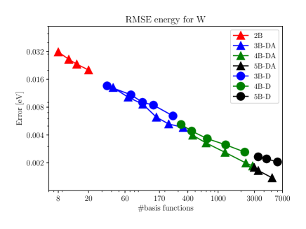
(a) Convergence of the RMS error on the energy for a tungsten database with distance-angle descriptors (triangles) and distance-based descriptors (circles).

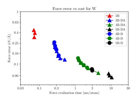
(b) Timing for the force evaluation per atom for a tungsten database with distance-angle descriptors (triangles) and distance-based descriptors (circles).

(c) Convergence of the RMS error on the energy for a silicon database with distance-angle descriptors (triangles) and distance-based descriptors (circles).

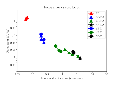
(d) Timing for the force evaluation per atom for a Silicon database with distance-angle descriptors (triangles) and distance-based descriptors (circles).

Figure 2: Systematic convergence on a tungsten (top) and a silicon (bottom) database. Note that the SOAP-GAP model takes about 30 ms / atom to evaluate on a range of current CPUs, and MTP is 1 ms or faster depending on the number of basis functions used.

II.5.2 Results for Silicon

We now demonstrate the convergence of the potential on a previously published silicon training set Bartók et al. (2018) which contains 2475 diverse configurations. We restrict the published database to train only on the following subset of configurations: diamond cubic, amorphous, $\beta$-tin, vacancies, sp2, and low index surfaces. The total amount of scalars included in the fit (total energies, force/virial components) for this subset of the silicon database is 323414. Although there are fewer configurations overall than in the tungsten database, there are two distinct solid phases, and the amorphous phase which is particularly challenging to fit. On the one hand, excluding certain parts of the published database allows us to explore extrapolation. On the other hand, efficiently and accurately fitting to the complete training set including a large variety of high coordination phases will likely require a more flexible functional form, which we will revisit in future work.

The full convergence tables are presented in the supplementary material sup .

As for tungsten, the choice of descriptors gives similar accuracy and evaluation times for silicon, but distance-angle potentials now reach significantly lower errors for large basis sets. Moreover, the convergence plots presented on Figures 2(c) and 2(d) show a systematic convergence of the energy error for distance-angle and distance-based descriptors. More precisely, the accuracy reaches the value of 2.13 meV accuracy for a distance-angle 4-body potential composed of 1933 basis functions with a force evaluation time of 3.32 ms per atom, and for a distance-based 5-body potential, the energy error reaches 2.49 meV composed of 5396 basis functions with a force evaluation time of 2.51 ms per atom. Finally, the 5-body distance-angle potentials reach an energy error of 1.47 meV with 3759 basis functions and a force evaluation time of 3.91 ms per atom.

III Regularisation

III.1 Regularisation Techniques

In the least-squares method, regularisation is primarily seen as a procedure to improve conditioning on ill-conditioned or even ill-posed problems. By contrast, in the Gaussian process framework, it can be interpreted as imposing ‘prior’ information about the potential energy surface, in particular its regularity. Robust heuristics for choosing the strength of the regularisation were crucial for the success of the GAP scheme for materials, where the regulariser was chosen to be consistent with the estimated convergence error in the input data e.g. with respect to k-point sampling Dragoni et al. (2018).

In the following we seek to apply a similar perspective in the standard least squares framework. We will show how the low-dimensional functional forms obtained in our definition of aPIPs in § II allow us to incorporate physically motivated ‘prior’ information or requirements that are not present in the database.

For example, consider the unregularised pair potential fit to the W database displayed in Figure 3(c), which is obtained by fitting a degree 16 polynomial with distance transform $u_{ij}=(2.74\text{\AA}/r_{ij})^{2}$ and cutoff radius $r_{\rm cut}=8.5\text{\AA}$; see § III.2 for more details. While it gives low RMSE on our dataset, it is a nonsensical pair potential that is unsuitable for materials modelling work.

A typical approach to detect overfitting and validate the generalisation capabilities of the fitted potential is to first separate the data into a training set and a test set, then to perform the regression using only the training set, and finally compute the errors separately on the training and on the test set. A transferable fit should have comparable training and test errors.

While such a procedure helps to prevent overfitting near the training set, we find that it gives very limited information about the ability of the potential to generalise more broadly. While training and test errors are comparable for a proportion of training configurations of 0.6 and higher (Figure 3(a)), all potentials exhibit an oscillatory shape (Figure 3(c)) which is pathological and clearly does not allow for extrapolation. In addition, the pair potential minimum is far from the nearest-neighbour distance. Therefore, the generalisation tests presented in Section IV are performed directly on physical properties and not using a training/test splits.

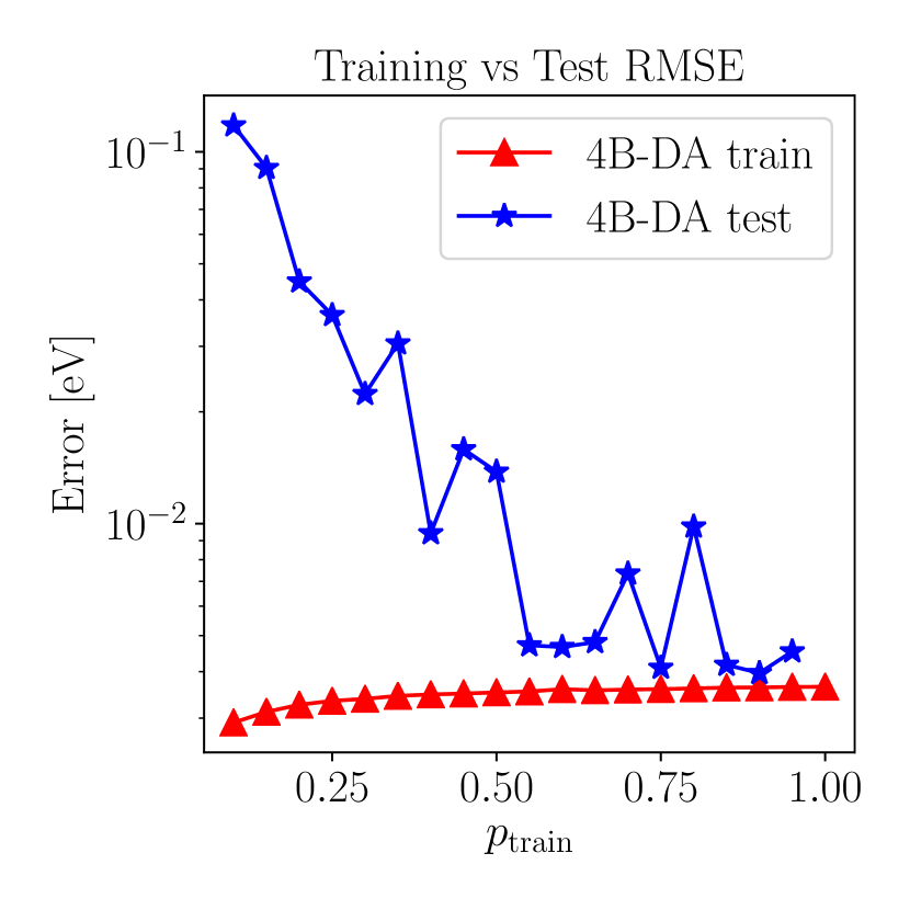
(a) Training and test errors for a series of unregularised 4B-DA potentials for tungsten. Here, $p_{\rm train}$ is the proportion of training configurations, chosen at random.
 

(b) Cumulative force error distribution on the entire tungsten training set. The aPIP potentials here correspond to $p_{\rm train}=1$ of the other panels, and the SOAP-GAP model is the one originally published with the data set.

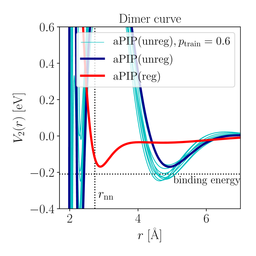
(c) Two-body part of the unregularised aPIP potentials with $p_{\rm train}=0.6$ (multiple curves correspond to different subsets) and $p_{\rm train}=1.0$, as well as the regularised potential; see § III.2 for the details.
 

Figure 3: Comparison of training and test errors, and the corresponding two-body potentials.

We now introduce a range of tools that enable us to produce regularised aPIP fits that retain RMSE accuracy close to the unregularised aPIPs, but become highly transferrable potentials that “extrapolate well” and in particular have no regions of “holes” as those described in Nandi et al. (2019).

III.1.1 Tikhonov regularisation

First, we recall some background on regularisation. In the context of linear least squares, the problem (10) is replaced with the regularised least squares problem

$$\min_{{\bf c}}\|A{\bf c}-Y\|_{2}^{2}+\|\Gamma{\bf c}\|_{2}^{2},$$ (12)

where $\Gamma$ is called the Tikhonov matrix. The form $\|\Gamma{\bf c}\|_{2}^{2}$ may be used to represent any positive quadratic functional acting on the aPIP potential energy surface $E$ given by (8). The most common choice is $\Gamma=\alpha I$ ($L^{2}$-regularisation) where the unknown parameter $\alpha$ may be obtained through ad hoc procedures, or related to the uncertainty of the data via the Bayesian interpretation of the least squares problem.

Such regularisation techniques are, for example, employed to render ill-posed problems well posed, or improve the conditioning of severely ill-conditioned problems. In our context, polynomial basis functions generally lead to ill-conditioning, which is exacerbated by the fact that the space of $n$-body functions contains $m$-body functions with $m<n$, leading to a near-degeneracy that is only partly alleviated by using of a different cut-off and distance transform at each body-order.

To solve the regularised least squares problem we re-interpret it as a standard least squares problem through the equivalent formulation

$$\min_{{\bf c}}\left\|\left[\begin{matrix}A\\ \Gamma\end{matrix}\right]{\bf c}-\left[\begin{matrix}Y\\ 0\end{matrix}\right]\right\|_{2}^{2},$$

which is then solved using the QR factorisation.

III.1.2 Rank-revealing QR factorisation

$L^{2}$-regularisation can be effectively replaced by the rank-revealing QR factorisation (rr-QR) Chan (1987), a decomposition which reveals the near-degeneracy of the matrix $A$. The factorisation reads

$$AP=Q\begin{pmatrix}R_{11}&R_{12}\\ 0&R_{22}\end{pmatrix},$$

where $P$ is a permutation matrix, $Q$ is an orthogonal matrix, $R_{11}$ and $R_{22}$ are upper triangular matrices and, importantly, a given norm of the matrix $R_{22}$ is below some prescribed tolerance.

Truncating $R_{22}$ in the resolution of the least-square system can be seen as a regularisation as it removes the small modes in the matrix $A$. To demonstrate this, let us compare rr-QR and $L^{2}$-regularisation on a simple example, where $A$ is the nearly rank-deficient matrix

$$A=\begin{pmatrix}1&0\\ 0&\varepsilon\end{pmatrix},\quad\varepsilon\mbox{ small,}$$

and the observations are $Y=(y_{1},y_{2})^{T}$. The solution of the unregularised least squares problem is $c_{1}=y_{1},c_{2}=y_{2}/\varepsilon$. The rr-QR algorithm with a parameter $\alpha$ will instead compute

$$c_{1}=y_{1},\quad c_{2}=\varepsilon^{-1}\delta_{\varepsilon>\alpha}y_{2},$$

while the least squares solution with $L^{2}$-regularisation with parameter $\alpha$ is given by

$$c_{1}=\frac{1}{1+\alpha^{2}}y_{1},\quad c_{2}=\frac{\varepsilon}{\varepsilon^{2}+\alpha^{2}}y_{2}.$$

The two solutions are asymptotically equivalent and tend to the unregularised solution as $\alpha\rightarrow 0$. In particular, the first coefficient is exactly right with the rr-QR factorisation but not with the Tikhonov regularisation.

III.1.3 Integral functionals

We now introduce a class of regularisers that are made possible by the fact that we decompose the PES into relatively low-dimensional components, the body-orders. A special case, discussed in the next section will be a critical ingredient in our fitting procedure.

Consider a PES given by a body-order expansion (1), and let us assume that we write $E_{n}$ as a distance-based or distance-angle potential, i.e., $E_{n}(\{{\mathbf{r}}_{i}\}_{i})=V_{n}({\bf u}_{n}(\{{\mathbf{r}}_{i}\}))$. Then we consider a regularisation functional of the form,

$$\|\Gamma_{n}{\bf c}\|^{2}_{2}=\int w({\bf u})\Big{|}L\big{[}V_{n}({\bf u})\big{]}\Big{|}^{2}\,d{\bf u},$$ (13)

where $L$ is a linear differential operator, $w$ an integration weight and integration is taken over the domain of definition of $V_{n}$, i.e., all admissible tuples ${\bf u}$ that can be written as ${\bf u}={\bf u}_{n}(\{{\mathbf{r}}_{i}\})$. The right-hand side can be written in the form of a Tikhonov functional since $V_{n}$ depends linearly on a subset of coefficients ${\bf c}$.

To approximately evaluate this integral we choose integration points $\{{\bf u}_{j}\}_{j=1}^{J}\subset{\mathbb{R}}^{d}$ that are distributed according to the measure $w({\bf u})d{\bf u}$ and replace the integral functional (13) with its discretised variant

$$\|\Gamma_{n}{\bf c}\|^{2}_{2}=\frac{1}{J}\sum_{j=1}^{J}\Big{|}L\big{[}V_{n}({\bf u}_{j})\big{]}\Big{|}^{2}.$$ (14)

A canonical choice for $\{{\bf u}_{j}\}_{j=1}^{J}$ are low-descrepancy sequences; we simply use the classical Sobol sequence. This is effective in low and moderate dimensions where Sobol sequences “fill space” with few (O(1000) to O(100,000)) points Niederreiter (1988). In principle one could also use random number sequences instead.

In Figure 4 we show how solid configurations are highly concentrated in the space of $n$-body clusters. Amorphous configurations “fill space” much better (liquid even more so), and can to a certain degree be seen as a “natural” regulariser, however they still concentrate in parts of configuration space. By contrast, random or Sobol sequences provide close to uniform distributions of datapoints at which to apply the regularisation, or alternatively their concentration can be easily tuned by adjusting the upper and lower bounds or through applying a distance transformation.

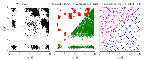
Figure 4: Distribution of 3-body clusters in the W and Si training sets versus artificially generated (random, Sobol) clusters.The clusters are represented by distance-angle variables $(r_{1},r_{2},w_{12})$ with the angle variable $w_{12}=\hat{R}_{1}\cdot\hat{R}_{2}$ restricted to $-0.3\leq w_{12}\leq-0.2$. The picture is similar for other angle-intervals.

III.1.4 Laplace smoother

A wide variety of choices for the differential operator $L$ in (14) are possible. In the present work we will only consider the Laplace operator, $L=\gamma\Delta\equiv\gamma\nabla^{2}$, i.e., (14) becomes

$$J_{n}^{\Delta}=\frac{\gamma_{n}}{J}\sum_{j=1}^{J}\Big{|}\Delta\big{[}V_{n}({\bf u}_{j})\big{]}\Big{|}^{2},$$ (15)

where $\gamma_{n}$ is an adjustable regularisation parameter. Although it is in principle possible to implement second derivatives of $V_{n}$, we have chosen instead to approximate $\Delta V_{n}$ with a finite-difference,

$$\begin{split}\Delta_{h}V_{n}({\bf u})=h^{-2}\sum_{\alpha=1}^{d}\Big{(}V_{n}({\bf u}+h{\bf e}_{\alpha})-2V_{n}({\bf u})&\\[-5.69054pt] +V_{n}({\bf u}-h{\bf e}_{\alpha})&\Big{)}\end{split}$$

Regularising the least squares fit with the functional $J_{n}^{\Delta}$ promotes that the curvature $\Delta V_{n}$ is moderate, which is a gentle requirement of smoothness. By adjusting the parameter $\gamma_{n}$, smoothness can be traded against accuracy of fit.

III.1.5 Two-sided cutoffs and repulsive core

For distances well below the nearest-neighbour distance regularisation is particularly crucial as demonstrated in Nandi et al. (2019) and in Figure 3(c). While we could apply the Laplace regulariser in this region to control oscillations of the polynomials and thus prevent “holes” in the PES, this would inhibit the ability of the polynomials to produce an accurate fit in regions of interest. Instead, we chose to (1) apply an inner cutoff to all $V_{n}$, $n\geq 3$; and (2) replace the global two-body polynomial $V_{2}$ with a spline that guarantees repulsion at short interatomic distances. In detail we apply these ideas as follows:

Two-sided cutoff:

Typically, the cutoff function $f_{\rm cut}$ appearing in (3) and (5) are positive on an interval $[0,r_{\rm cut})$ and vanish on $[r_{\rm cut},\infty)$. For example, we often use the spline defined in (11).

In order to prevent oscillation and blow-up of the $n$-body functions $V_{n}$, $n\geq 3$ we require that $f_{\rm cut}=0$ on both $[0,r_{\rm cut}^{\prime}]$ and $[r_{\rm cut},\infty)$. A specific choice that we used in our tests is

$$\begin{split}f_{\rm cut}(r)&=\begin{cases}C\big{(}\xi^{2}-1\big{)}^{2},&r_{\rm cut}^{\prime}<r<r_{\rm cut},\\ 0,&\text{otherwise},\end{cases}\\ \xi&=\exp\Big{(}\lambda\big{(}r/r_{\rm nn}-1\big{)}\Big{)}-1,\end{split}$$ (16)

where $r_{\rm nn}$ is an estimate for the ground state nearest neighbour distance in the material under consideration, $\lambda$ is chosen such that the resulting $f_{\rm cut}$ has its unique local maximum at $r_{\rm nn}$ and $C$ such that $f_{\rm cut}(r_{\rm nn})=1$. See Figure 5 to visualise this construction. We emphasize, however, that there are many reasonable alternatives to implement this.

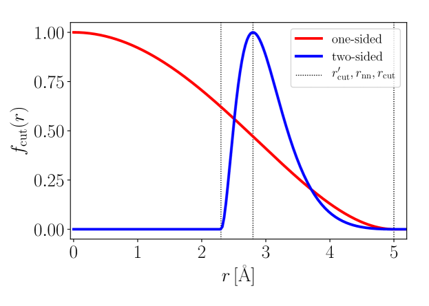
Figure 5: A one-sided cutoff function (11) for the two-body function $V_{2}$ and a two-sided cutoff function (16) for $n$-body functions $V_{n}$, $n\geq 3$. The illustrative parameters are $r_{\rm cut}^{\prime}=2.3\text{\AA},r_{\rm nn}=2.8\text{\AA},r_{\rm cut}=5.0\text{\AA}$.

Repulsive Two-Body:

We initially perform the regularised least-squares fit with a global polynomial representation of $V_{2}$ as described in § II. We then choose a spline point $r_{\rm S}<r_{\rm nn}$, sufficiently small so that modifying $V_{2}(r)$ for $r<r_{\rm S}$, ideally chosen small enough so that the RMSEs are not significantly affected. This point must furthermore be chosen so that $V_{2}^{\prime}(r_{\rm S})<0$. We then define a new two-body potential

$$\tilde{V}_{2}(r) :=\begin{cases}V_{2}(r),&r\geq r_{\rm S},\\ V_{\rm rep}(r),&r<r_{\rm S},\end{cases}$$

$$V_{\rm rep}(r) =e_{\infty}+\beta r^{-1}e^{-\alpha r},$$

where $e_{\infty}<V_{2}(r_{\rm S})$ is a tuning parameter that can be used to adjust the steepness of the potential, while $\alpha,\beta$ are chosen such that $\tilde{V}_{2}$ is continuous and continuously differentiable at $r_{\rm S}$. The form of the repulsive potential $V_{\rm rep}$ is arbitrary, and in applications where it is important to accurately describe interactions between atoms at very close distances it should be chosen as or similar to the universal ZBL function Ziegler et al. (1985). The repulsive core constructions for the regularised W and Si fits, described in detail in § III.2, are visualised in Figure 6.

Figure 6: Spline two-body potentials with repulsive core; cf. § III.1.5(b).

In practice, the inner cutoff and splining mechanisms interact mildly with the regularised least squares regression, and we did not find it particularly difficult to find suitable parameter choices.

III.1.6 Sequential Fits

A source of ill-conditioning in the least squares system (10) is due to the fact that any $m$-body function $V_{m}$ can nearly be represented as an $n$-body function $V_{n}$ with $n>m$. Thus, a final mechanism that we employ is to fit different $n$-body terms independently from one another. For example, we may first fit a two-body $V_{2}$, followed by the modification described in § III.1.5(2). Then, in a separate step we fit $V_{3},V_{4}$, and possibly $V_{5}$ after subtracting the values for $V_{2}$ from the observations vector. At present we perform this procedure in a purely ad hoc fashion.

III.2 Accuracy of Regularised aPIPs

In this section, we investigate the effect of our regularisation procedures on the fit accuracy for the W and Si training sets described in § II.5, as well as a small selection of material properties. While the Si fits will be performed with a 5-body potential, for the W potential we restrict the body-order to four since this already achieves satisfactory accuracy on the W training set.

The majority of hyperparameters for the Si and W fits are identical and can be summarized as follows: All potentials are distance-angle potentials with the same distance transforms $u_{ij}$ as in the RMSE convergence tests. For the unregularised aPIPs the cutoff function is (11) while for the regularised aPIPs we use the one-sided cutoff (11) only for the two-body potential but a two-sided cutoff (16) for all $V_{n},n\geq 2$. The least squares functionals are weighted differently from the RMSE convergence tests where we were targeting total RMSEs. For the regularisation and extrapolation tests we chose the weights to aim for accuracy on subsets comparable to the previously published SOAP-GAP models. The regularised fits employ the complete range of tools introduced in § III.1. The specific details of the aPIP potential parameters, fitting parameters and regularisation parameters, and sequential fitting procedure, are given in the supplement.

The resulting unregularised and regularised potentials will, respectively, be denoted by aPIP(unreg) and aPIP(reg).

III.2.1 Results: Tungsten

We compare the aPIP RMSE for energies, forces and virials per configuration type in the tungsten training set against the original SOAP-GAP model published with the data set Szlachta et al. (2014). The results can be found in Table 4. The purpose of this test is to confirm that the regularisation only slightly reduces the RMSE accuracy per atom compared to the unregularised aPIP(unreg).

Apart from monitoring the RMSE we also benchmark the fitted potentials by comparing their predictions for various material properties: energy-volume curves of the aPIP models as well as the SOAP-GAP model are compared against DFT in Figure 7. These results are shown to be in excellent agreement for all the fitted potentials. A second test is to calculate the elastic constants $B$, $C_{11}$, $C_{12}$, $C_{44}$ for a bcc tungsten structure. The aPIP(unreg), aPIP(reg) and SOAP-GAP all achieve to predict the elastic constants within 1$\%$.

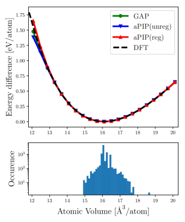
Figure 7: Tungsten bcc energy versus volume comparing SOAP-GAP Szlachta et al. (2014) against regularised and unregularised aPIP. The lower panel shows the histogram of volumes in the data set.

	Energy [meV]			Forces [meV/Å]			Virials [meV]
config type	GAP	aPIP(unreg)	aPIP(reg)	GAP	aPIP(unreg)	aPIP(reg)	GAP	aPIP(unreg)	aPIP(reg)
unit cells	0.07	0.24	0.27	0.00	0.00	0.00	3.47	3.80	4.17
bulk MD	0.60	0.47	0.45	27.8	21.4	26.5
vacancy	0.50	0.26	0.67	29.4	25.3	29.5
dislocation	1.86	0.98	1.02	38.3	33.0	35.7
surface	0.45	0.43	0.88	50.9	42.2	70.8
$\gamma$-surface	1.66	2.92	4.09	69.0	99.4	118.0
$\gamma$-s. vacancy	1.26	1.70	2.71	79.3	98.7	109.3

Table 4: RMSE Accuracy on W training set, comparing SOAP-GAP Szlachta et al. (2014) against regularised and unregularised aPIP.

III.2.2 Results: Silicon

The RMSE accuracy per configuration type of unregularised aPIP(unreg) and regularised aPIP(reg) are compared against the SOAP-GAP fitBartók et al. (2018) in Table 5. Again the regularised aPIP(reg) is shown to decrease in RMSE accuracy compared to the unregularised aPIP(unreg), and by larger factors than in the case of tungsten.

	Energy [meV]			Forces [meV/Å]			Virials [meV]
config type	GAP	aPIP(unreg)	aPIP(reg)	GAP	aPIP(unreg)	aPIP(reg)	GAP	aPIP(unreg)	aPIP(reg)
dia	0.65	0.33	0.55	15.4	13.9	21.8	14.59	6.09	9.96
amorph	0.56	2.08	4.49	102.7	138.6	172.0	60.9	15.85	31.32
bt	0.72	0.27	0.45	17.2	18.2	31.2	26.47	12.94	22.15
vacancy	0.54	0.36	0.71	48.3	46.2	62.7	9.82	7.52	11.89
sp2	0.48	0.70	1.82	48.6	45.0	79.2
surface110	0.20	0.48	2.80	161.2	159.0	237.0
surface111	0.22	0.31	0.99	156.9	155.8	233.7
surface001	0.19	0.50	1.39	140.4	136.9	195.7

Table 5: RMSE Accuracy on Si training set, comparing SOAP-GAP Bartók et al. (2018) against regularised and unregularised aPIP.

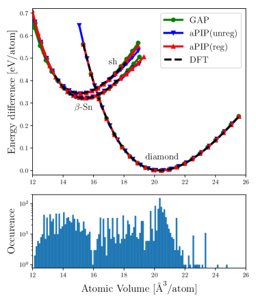
Figure 8: Energy volume curve for diamond and $\beta$-Sn silicon comparing the regularised and unregularised aPIPs, and SOAP-GAP potentials against DFT. The lower panel shows the histogram of the volumes in the data set.

The fitted potentials were again compared for a range of different material properties. The energy versus volume curve for silicon is shown in Figure 8 comparing the fitted potentials to the DFT reference, with excellent agreement for each. The elastic constants were calculated as well as the surface and vacancy formation energies and are presented in Table 6. The unregularised aPIP(unreg) is shown to have larger errors on the elastic constants compared to the aPIP(reg) and most notably failed the vacancy energy test. That is, during the relaxation of the vacancy using the aPIP(unreg) potential the optimiser failed to find a local minimiser. This is a manifestation of “holes” in the fit which will be discussed in § III.3. In comparison to SOAP-GAP the aPIP(reg) performs well in calculating the elastic constants and vacancy formation energy. The aPIP(reg) performs worse in the surface formation energies, most specifically the (111) direction, which we believe can only be rectified by using even higher body order terms. Implementing this efficiently is a focus of future work.

Model	Elastic Constants [GPa]				Surface Energy [J / m2]			Point defect [eV]
	B	$C_{11}$	$C_{12}$	$C_{44}$	(100)	(110)	(111)	vacancy
DFT	87.45	152.21	55.07	74.95	2.17	1.52	1.57	3.67
Relative Error ($\%$)
GAP	$<$1	-3	3	-7	-1	-1	-3	-2
aPIP(unreg)	8	5	12	-1	-6	-2	-5	-
aPIP(reg)	$<$1	3	-5	-4	-3	-3	-10	-4

Table 6: Relative error on a range of different properties for Si, comparing the SOAP-GAP, aPIP and aPIP(reg) potentials. The unregularised aPIP failed the vacancy test.

III.3 Holes

As a first test of the “transferability” of our regularised aPIP fits we determine whether the resulting potentials have any “holes” in the sense of Nandi et al. (2019): regions of unphysically low potential energy values. The importance of avoiding such behaviour is hard to overstate: in most molecular modelling applications, samples will be drawn using the model distribution, and due to the exponential amplification of the Boltzmann distribution at low and moderate temperature, holes can lead to catastrophic failure of models.

Having decomposed the total PES into low-dimensional components gives the option of searching for low-energy configurations in these individual components $V_{n}$. Specifically, we choose a minimal inner distance $r_{0}<r_{\rm cut}^{\prime}$, i.e., below the inner cutoff. Then, for each $n$-body term $V_{n}$ we compute an approximate minimum of $V_{n}({\mathbf{r}}_{1},\dots,{\mathbf{r}}_{n})$ over all clusters $({\mathbf{r}}_{1},\dots,{\mathbf{r}}_{n})$ with $r_{0}\leq r_{j}\leq r_{\rm cut}$, using Sobol sequences with a few million points. The results are summarized in Table 7. It is interesting to note that the “holes” in the unregularised Si fit are less severe. We speculate that this is due to the fact that the Si training set is much richer; cf. Figure 9.

		$\inf V_{n}$
	$~{}~{}n~{}~{}$	aPIP(unreg)	aPIP(reg)
W	2	-273 eV	-0.08 eV
	3	-192359 eV	-0.06 eV
	4	-4877 eV	-0.18 eV
Si	2	-0.66 eV	-0.08 eV
	3	-2934 eV	-0.6 eV
	4	-447 eV	-0.11 eV

Table 7: “Holes” in the unregularised aPIP(unreg) potentials.

In the unregularised fit we visualise the location of holes by plotting slices through the $V_{3}$ energy landscape in Figure 9. This shows in particular that holes appear both in regions of large angles and moderate angles near the ground-state.

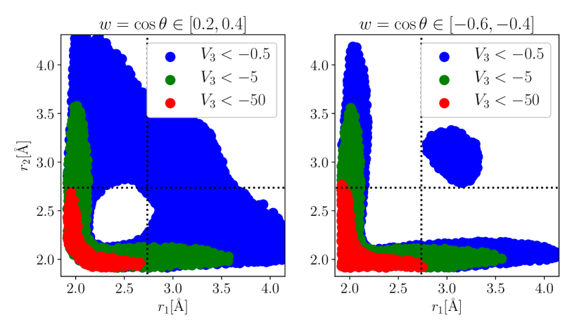
Figure 9: Holes in the 3-body potential $V_{3}$ for the unregularised W aPIP fit. Two slices through the potential energy landscape are plotted.

IV Generalisation

This section presents a series of tests to benchmark the generalisation performance of the aPIP and GAP models against a DFT reference. These tests were designed to probe configurational space far from the training data region and monitor each models’ performance. We use the term “generalisation” (also often called “extrapolation” or “transferability”) in a loose sense and simply take it to mean “evaluation far from the training set” which may technically also include interpolation—the distinction is tenuous in high dimension.

IV.1 Tungsten

IV.1.1 Interstitial

The tungsten aPIP(unreg) and aPIP(reg) models introduced in III.2.1 were compared against the original SOAP-GAP model Szlachta et al. (2014) and a DFT reference for the self-interstitial defect. The DFT parameters were chosen to be identical to those used in the original paper. These settings were: 600 eV cutoff energy, 0.03 Å^-1 kpoint spacing and 0.1 eV smearing width. The training set does not include interstitial data; cf. Table 4. We formed the interstitial defect by inserting an atom in a DFT relaxed 54 atom tungsten bcc cell at the octahedral site ($\frac{1}{2}$, 0, 0) of the primitive cell. The geometry was then relaxed using DFT. A linear path between the unrelaxed and relaxed configurations was created and the DFT, SOAP-GAP and aPIP models were evaluated along this path and are shown in Figure 10.

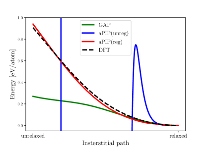
Figure 10: Linear path between unrelaxed and relaxed tungsten interstitial configuration. The unregularised aPIP fit explodes whereas the regularised aPIP closely matches the DFT reference.

This interstitial test probes small interatomic distances which are not contained in the training database and can therefore be strictly seen as an extrapolation test. Due to the smoothness prior, the SOAP-GAP model underestimates the energy difference along the interstitial path compared to the DFT reference. As expected, the unregularised aPIP model heavily oscillates along this test path since it explores configurations it was not fitted to. By contrast, the combination of integral regularisers, repulsive core and inner cut-offs result in a regularised aPIP model that shows an excellent match to the DFT curve. The level of agreement is likely fortuitous, but we expect that in general the correct repulsive nature of the potential is obtained due to having enforced this property in the two body function $V_{2}$.

IV.2 Silicon

IV.2.1 Surface Decohesion

We set up a bulk Si diamond 10x1x1 supercell and increase the lattice vector length in the long direction while keeping the atomic positions fixed which in turn creates two surfaces Bartók et al. (2018). Both the initial bulk structure and final surfaces are configurations that are well represented in the training set and fitted by the aPIP(unreg), aPIP(reg) and SOAP-GAP models to within 3 meV accuracy; cf. Table 5. The configurations along the path in between are not contained in the database. Therefore this test can be seen as generalising in that it evaluates the potential on a path between two accurately fitted configurations.

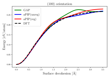
Figure 11: Decohesion curve in silicon bulk diamond along the $(100)$ direction. The bulk diamond structure corresponds to the left end and the unrelaxed $(100)$ surface is on the right.

Figure 11 shows that the end points, bulk diamond and (100) surface, are accurately fitted. However, the SOAP-GAP has a local maximum around 2.5 Å, unlike the DFT reference which shows a smooth and monotone transition along this path, a characteristic which both the aPIP(unreg) and aPIP(reg) mimic more accurately than SOAP-GAP.

IV.2.2 Layer Test

In this test we set up a bulk silicon diamond configuration and and gradually increase the interplanar spacing between the $(111)$ layers of silicon. The configurations along this path are arguably unphysical but should, as the DFT model confirms, correspond to unstable high energy configurations. Past experience shows that poorly fitted potentials can have unphysically low energies for such configurations. The aPIP and SOAP-GAP models were evaluated on this path and are compared to the DFT reference in Figure 12.

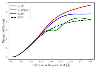
Figure 12: The layer test along which bulk silicon is split in layers of silicene. The SOAP-GAP model predicts a high energy local minima whereas the regularised aPIP model does not.

The SOAP-GAP model predicts a high energy local minimum along this path, which should be entirely unstable as shown by the DFT reference. The presence of such false high energy local minima are detrimental for applications such as random structure search Pickard and Needs (2011) but also high temperature or high stress molecular dynamics. The aPIP(unreg) model has a much more shallow high energy local minimum, but the aPIP(reg) model show no minimum at all (while still not being quantitatively accurate in the unphysical region).

IV.3 Titanium

Titanium is a difficult material to construct interatomic potentials for, due to its bonding chemistry being intermediate between covalent and metallic and we therefore chose it for our final test system. Here we want to explore how the different functional forms and regularisation strategies perform in the limit of very little data. The motivation for this is partly that the large size of the published data sets in the previous sections in and of itself acts like a regulariser, but also that in the future we wish to eliminate extensive sampling as a way to generate data sets. Rather, we would like to develop potential fitting frameworks that are explicitly regularised to the extent that a few judiciously chosen training configurations are sufficient to obtain good interatomic potentials.

We generated two very limited training sets, denoted by Set 1 and Set 2. To Set 1, we fit unregularised and regularised aPIP potentials denoted, respectively, by ${\rm aPIP}_{1}{\rm(unreg)}$ and ${\rm aPIP}_{1}{\rm(reg)}$, as well a SOAP-GAP potential denoted GAP₁. In addition we fit an unregularised aPIP potential, denoted aPIP₂ (unreg) to Set 2. The detailed potential and fitting parameters are described in the supplementary information.

Set 1

This set contains primitve cell bcc and hcp configurations, obtained by sampling the Boltzmann distribution with a temperature parameter set to 100 K as the lattice vectors (and in case of bcc, the relative positions of the two atoms) are varied. The obtained configurations were evaluated using CASTEP Clark et al. (2005) with k-point spacing set to 0.015 Å^-1, 750 eV cutoff energy and 0.1 eV smearing width. In addition 3x3x3 bcc and hcp supercells were added, and Phonopy Togo and Tanaka (2015) was used to generate the inequivalent finite displacements (one for each structure) of a single atom by a magnitude of 0.001 Å. These two configurations were evaluated with a larger k-point spacing equal to 0.03 Å^-1.

Set 2

This set contains Set 1 as well as additional finite displacement configurations analogous to those in Set 1, but now with a 0.01 Å displacement.

IV.3.1 Cohesive energy

Figure 13 shows the energy versus volume curves for the titanium bcc and hcp phases for the various potentials all fitted to Set 1. The distribution of the atomistic volumes are on the lower panel and show that training data covers only volumes in the range between 15 and 17 ų/atom. In this region both aPIP models as well as the GAP model agree well with the DFT reference. For smaller and larger volumes the fitted potentials all deviate from the DFT reference as expected due to the lack of data. However, the unregularised aPIP shows a steep drop for small volumes and a second minimum for large volumes whereas the regularised aPIP and GAP mimic the DFT curve at least qualitatively, showing the benefits of regularisation.

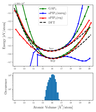
Figure 13: Energy versus volume plots for Titanium hcp and bcc phase. The volume histogram below shows the distribution of the training data.

IV.3.2 Phonon spectrum

SOAP-GAP and aPIP models fitted to Set 1 and Set 2 were used to generate the phonon spectra for bcc and hcp titanium and are compared to the DFT reference in Figure 14. Although aPIP₁(unreg) and aPIP₁(reg) were both fitted to Set 1, aPIP₁(unreg) failed catastrophically while aPIP₁(reg) produces a highly accurate phonon spectrum. The negative frequencies of the bcc phonon spectrum at the $\Gamma$ points demonstrates the instability of the structure at 0 K.

Of course an alternative, but much less controllable way to improve the regularity of a potential is to simply add more data to the training set. ML potentials in the literature, even if they are not explicitly regularised, can avoid the unphysical behaviour seen in here because they are fitted to large data sets. To see this effect, consider the potentials fitted to Set 2: aPIP₂(unreg) phonon spectra are somewhat improved, but they remain highly inaccurate quantitatively. We expect that much more training data would be required to accurately converge the phonon spectrum of an unregularised potential. We suggest instead that regularisation and a single displacement per crystal structure are enough to accurately reproduce phonon spectra.

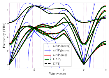
(a) Titanium hcp phonon spectrum

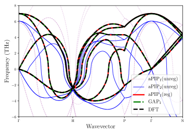
(b) Titanium bcc phonon spectrum

Figure 14: Phonon spectra computed using the aPIP, SOAP-GAP models and DFT reference. Regularisation increases the accuracy of the aPIP models, similarly to the addition of FDC data.

IV.3.3 Burgers’ path

The Burgers’ path is a pathway from the bcc to hcp crystal structure Burgers (1934). It consists of a shear deformation applied to the bcc structure followed by a shuffle of atomic layers resulting in a hcp structure Caspersen et al. (2004).

We evaluated the Set 1 fits on the Burgers’ path and the results are plotted against the DFT reference in Figure 15. The energy per atom along the Burgers’ path shows that the SOAP-GAP model overestimates the barrier by 30 meV along the transition from bcc to hcp. The aPIP models as well as the DFT reference do not show such a barrier. The training database contains bcc/hcp configurations sampled at a low temperature (T=100 K) resulting in a database containing structures close to the relaxed bcc and hcp configurations. As expeced, Figure 15 shows the aPIP and SOAP-GAP models both predict the energies for the hcp and bcc crystals accurately. However, the aPIP model manages to predict the energy along the middle part of the path more accurately compared to the DFT reference.

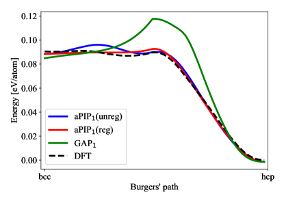
Figure 15: Burgers’ path comparing aPIP, SOAP-GAP and DFT reference. The SOAP-GAP model correctly predicts the relaxed bcc/hcp energies at both ends of the path but overestimates the energy along the remainder of the path.

To analyse this we use body order expansion to investigate the Burgers’ path test in a different way. By plotting the 3-body distances $r_{12}$, $r_{13}$, $r_{23}$ of the primitive cell training database, Set 1, we can visualise the clustering of data in the $V_{3}$ space. Figure 16 shows the clustering of data around the relaxed bcc/hcp configurations and shows the Burgers’ path connecting the two configurations as well. The training data was sampled at a low temperature (T=100K) and we therefore see a limited exploration of data away from the relaxed configurations. The Burgers’ path clearly explores configurations in this $V_{3}$ space where there is little to no data present, showing that even in this low dimension this test can be considered as a non-trivial generalisation.

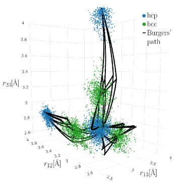
Figure 16: Visualisation of the sparsity of the Ti training sets: each datapoint represents a 3-body cluster, described through interatomic distances $r_{12},r_{13},r_{23}$, contained in the primitive cell configurations of Set 1. The Burgers’ path explores regions of 3-body space far from the regions with datapoints, which demonstrates that the Burgers’ path test requires significant generalisation away from the training set.

We believe that the lack of accuracy along the Burgers’ path of SOAP-GAP model is due to the lack of training data in that region. It is a manifestation of high dimensional fits giving answers that are still regular, but have uncontrolled errors when extrapolating away from the training database. The aPIP models perform significantly better in this test because, as we propose, models fitted in low dimension (e.g. the dimensionality of the body orders) will in general perform better in generalisation tests compared to high dimensional fits such as SOAP-GAP models.

It will also be interesting to systematically explore the relative benefits and possible unification of regularisation and active-learning style techniques that bring in new data in previously unexplored regionsNandi et al. (2019); Podryabinkin and Shapeev (2017).

V Conclusion

The purpose of this paper was two-fold: Firstly, we developed atomic PIPs (aPIPs), a generalisation of PIPs Braams and Bowman (2009), interatomic potentials constructed from permutation invariant polynomials for material systems by applying the PIP construction to atomic body ordered expansions of the total energy and endowing them with usual cutoff mechanisms. By fitting the polynomial coefficients to solid training sets (rather than clusters in vacuum) we were able to obtain an accuracy comparable with the SOAP-GAP models for tungsten Szlachta et al. (2014) and silicon Bartók et al. (2018) (on a non-trivial subset of the full training set) using low body-orders, four or five, which are still at least an order of magnitude faster to evaluate than SOAP-GAP.

Secondly, we studied the generalisation (extrapolation) properties of the aPIPs. We developed novel regularisation mechanisms that exploit the low-dimensional structure of the body-ordered terms to ensure correct qualitative behaviour of the potentials, such as smoothness, well away from the training set. We showed that such a regularisation is crucial to achieve the extrapolation properties of the Gaussian process based SOAP-GAP Szlachta et al. (2014); Bartók et al. (2018). Indeed, our regularisation techniques are amenable to fine-tuning which enabled us to significantly improve on the SOAP-GAP model in several tests. Thus, we have established that our framework provides a novel “tool kit” for fitting interatomic potentials for materials with high accuracy and excellent transferability, across a wide range of bonding chemistries.

The silicon, tungsten and titanium datasets are openly available at http://www.libatoms.org/Home/DataRepository, the aPIP framework can be found at https://github.com/cortner/NBodyIPs.jl.

VI Acknowledgements

GC and C. vd O. acknowledge the support of UKCP grant number EP/K014560/1. C. vd O. would like to acknowledge the support of EPSRC (Project Reference: 1971218) and Dassault Systèmes UK. CO and GD are supported by Leverhulme Research Project Grant RPG-2017-191.

References

- Finnis (2004) M. Finnis, Progress in Materials Science 49, 1 (2004).
- Parr (1980) R. G. Parr, in Horizons of Quantum Chemistry, edited by K. Fukui and B. Pullman (Springer Netherlands, Dordrecht, 1980) pp. 5–15.
- Ercolessi and Adams (1994) F. Ercolessi and J. B. Adams, EPL (Europhysics Letters) 26, 583 (1994).
- Murrell (1984) J. N. Murrell, Molecular potential energy functions (J. Wiley, 1984).
- Atkins and Friedman (2011) P. Atkins and R. Friedman, Molecular Quantum Mechanics (OUP Oxford, 2011).
- Huang et al. (2005) X. Huang, B. J. Braams, and J. M. Bowman, The Journal of Chemical Physics 122, 044308 (2005).
- Jain et al. (1996) A. K. Jain, Jianchang Mao, and K. M. Mohiuddin, Computer 29, 31 (1996).
- Bishop (2006) C. M. Bishop, Pattern Recognition and Machine Learning (Information Science and Statistics) (Springer-Verlag, Berlin, Heidelberg, 2006).
- Behler and Parrinello (2007) J. Behler and M. Parrinello, Phys. Rev. Lett. 98, 146401 (2007).
- Rasmussen and Williams (2005) C. E. Rasmussen and C. K. I. Williams, Gaussian Processes for Machine Learning (Adaptive Computation and Machine Learning) (The MIT Press, 2005).
- Bartók and Csányi (2015) A. P. Bartók and G. Csányi, Int. J. Quantum Chem. 115, 1051 (2015).
- Bartók et al. (2013) A. P. Bartók, R. Kondor, and G. Csányi, Physical Review B 87, 184115 (2013).
- Bartók et al. (2018) A. P. Bartók, J. Kermode, N. Bernstein, and G. Csányi, Physical Review X 8, 041048 (2018).
- Partridge and Schwenke (1997) H. Partridge and D. W. Schwenke, The Journal of Chemical Physics 106, 4618 (1997).
- Bramley and Carrington Jr. (1993) M. J. Bramley and T. Carrington Jr., The Journal of Chemical Physics 99, 8519 (1993).
- Cencek et al. (2008) W. Cencek, K. Szalewicz, C. Leforestier, R. van Harrevelt, and A. van der Avoird, Phys. Chem. Chem. Phys. 10, 4716 (2008).
- Xie et al. (2005) Z. Xie, B. J. Braams, and J. M. Bowman, The Journal of Chemical Physics 122, 224307 (2005).
- Babin et al. (2013) V. Babin, C. Leforestier, and F. Paesani, Journal of Chemical Theory and Computation 9, 5395 5403 (2013).
- Qu et al. (2018) C. Qu, Q. Yu, and J. M. Bowman, Annual Review of Physical Chemistry 69, 151 (2018).
- Griebel (2006) M. Griebel, in Foundations of Computational Mathematics (FoCM05), Santander, edited by L. Pardo, A. Pinkus, E. Suli, and M. Todd (Cambridge University Press, 2006) pp. 106–161.
- Rabitz and Aliş (1999) H. Rabitz and Ö. F. Aliş, J. Math. Chem. 25, 197 (1999).
- Stillinger and Weber (1985) F. H. Stillinger and T. A. Weber, Phys. Rev. B Condens. Matter 31, 5262 (1985).
- Nguyen et al. (2018) T. T. Nguyen, E. Székely, G. Imbalzano, J. Behler, G. Csányi, M. Ceriotti, A. W. Götz, and F. Paesani, J. Chem. Phys. 148, 241725 (2018).
- Glielmo et al. (2018) A. Glielmo, C. Zeni, and A. De Vita, Phys. Rev. B: Condens. Matter Mater. Phys. (2018).
- Sharma et al. (2006) A. R. Sharma, J. Wu, B. J. Braams, S. Carter, R. Schneider, B. Shepler, and J. M. Bowman, J. Chem. Phys. 125, 224306 (2006).
- Rupp et al. (2012) M. Rupp, A. Tkatchenko, K.-R. Müller, and O. A. von Lilienfeld, Phys. Rev. Lett. 108, 058301 (2012).
- Huo and Rupp (2017) H. Huo and M. Rupp, arXiv:1704.06439 (2017).
- Behler (2017) J. Behler, Angewandte Chemie International Edition 56, 12828 (2017).
- Behler (2011) J. Behler, The Journal of Chemical Physics 134, 074106 (2011).
- Deringer and Csányi (2017) V. L. Deringer and G. Csányi, Physical Review B 95, 094203 (2017).
- Nandi et al. (2019) A. Nandi, C. Qu, and J. M. Bowman, Journal of Chemical Theory and Computation 15, 2826 (2019).
- Shapeev (2016a) A. V. Shapeev, Multiscale Modeling & Simulation 14, 1153 (2016a).
- Drautz (2019) R. Drautz, Phys. Rev. B 99, 014104 (2019).
- Bartók et al. (2010) A. P. Bartók, M. C. Payne, R. Kondor, and G. Csányi, Physical review letters 104, 136403 (2010).
- Thompson et al. (2015) A. Thompson, L. Swiler, C. Trott, S. Foiles, and G. Tucker, Journal of Computational Physics 285, 316 (2015).
- Moriarty (1977) J. A. Moriarty, Phys. Rev. B 16, 2537 (1977).
- Moriarty (1982) J. A. Moriarty, Phys. Rev. B 26, 1754 (1982).
- Moriarty (1988) J. A. Moriarty, Phys. Rev. B 38, 3199 (1988).
- Nelson et al. (2013) L. J. Nelson, V. Ozoliņš, C. S. Reese, F. Zhou, and G. L. Hart, Physical Review B 88, 155105 (2013).
- Braams and Bowman (2009) B. J. Braams and J. M. Bowman, Int. Rev. Phys. Chem. 28, 577 (2009).
- Qu and Bowman (2019) C. Qu and J. M. Bowman, J. Chem. Phys. 150, 141101 (2019).
- Shapeev (2016b) A. Shapeev, Multiscale Model. Simul. 14, 1153 (2016b).
- Derksen and Kemper (2015) H. Derksen and G. Kemper, Computational Invariant Theory (Springer, 2015).
- Qu et al. (2013) C. Qu, R. Prosmiti, and J. M. Bowman, Theor. Chem. Acc. 132, 1413 (2013).
- Schmelzer and Murrell (1985) A. Schmelzer and J. N. Murrell, Int. J. Quantum Chem. 28, 287 (1985).
- Bosma et al. (1997) W. Bosma, J. Cannon, and C. Playoust, J. Symbolic Comput. 24, 235 (1997).
- (47) See Supplementary Material at link for a description of the 5-body invariants, convergence tables for tungsten and silicon, and details on the titanium database generation and parameters.
- Szlachta et al. (2014) W. J. Szlachta, A. P. Bartók, and G. Csányi, Phys. Rev. B Condens. Matter 90, 104108 (2014).
- Clark et al. (2005) S. J. Clark, M. D. Segall, C. J. Pickard, P. J. Hasnip, M. I. J. Probert, K. Refson, and M. C. Payne, Zeitschrift fur Kristallographie 220, 567 (2005).
- Dragoni et al. (2018) D. Dragoni, T. D. Daff, G. Csányi, and N. Marzari, Physical Review Materials 2, 1939 (2018).
- Chan (1987) T. F. Chan, Linear Algebra Appl. 88-89, 67 (1987).
- Niederreiter (1988) H. Niederreiter, Journal of Number Theory 30 (1988).
- Ziegler et al. (1985) J. F. Ziegler, J. P. Biersack, U. Littmark, and Others, “The stopping and range of ions in solids, vol. 1,” (1985).
- Pickard and Needs (2011) C. J. Pickard and R. J. Needs, Journal of Physics: Condensed Matter 23, 053201 (2011).
- Togo and Tanaka (2015) A. Togo and I. Tanaka, Scripta Materialia 108, 1 (2015).
- Burgers (1934) W. Burgers, Physica 1, 561 (1934).
- Caspersen et al. (2004) K. J. Caspersen, A. Lew, M. Ortiz, and E. A. Carter, Physical review letters 93, 115501 (2004).
- Podryabinkin and Shapeev (2017) E. V. Podryabinkin and A. V. Shapeev, Comput. Mater. Sci. 140, 171 (2017).