Extendability of functions with partially vanishing trace

Abstract.

Let $\Omega\subseteq\mathbb{R}^{d}$ be open and $D\subseteq\partial\Omega$ be a closed part of its boundary. Under very mild assumptions on $\Omega$, we construct a bounded Sobolev extension operator for the Sobolev space $\mathrm{W}^{k,p}_{D}(\Omega)$, $1\leq p<\infty$, which consists of all functions in $\mathrm{W}^{k,p}(\Omega)$ that vanish in a suitable sense on $D$. In contrast to earlier work, this construction is global and not using a localization argument, which allows to work with a boundary regularity that is sharp at the interface dividing $D$ and $\partial\Omega\setminus D$. Moreover, we provide homogeneous and local estimates for the extension operator. Also, we treat the case of Lipschitz function spaces with a vanishing trace condition on $D$.

1. Introduction

Sobolev spaces $\mathrm{W}^{k,p}_{D}(\Omega)$ that contain functions that only vanish on a portion $D$ of the boundary of some given open set $\Omega\subseteq\mathbb{R}^{d}$ play an eminent role in the study of the mixed problem for second-order elliptic operators, see for example [2, 4, 8, 9, 10, 12, 11, 13, 18, 23, 24]. In the study of these spaces, an extension operator is a crucial tool.

Early contributions to the history of Sobolev extension operators include the works of Stein [22, pp. 180–192] and Calderón [5] on Lipschitz domains as well as the seminal paper of Jones [20] on $(\varepsilon,\delta)$-domains. The latter mentioned work was later refined by Chua [6] and Rogers [21]. Even though all these constructions aim at the full Sobolev space $\mathrm{W}^{1,p}(\Omega)$, they restrict to bounded extension operators on the space with vanishing trace on $D$ and the extensions preserve the trace condition on $D$ if a mild regularity assumption is imposed, see [3, Lem. 3.4].

All these constructions rely on regularity assumptions for the full boundary of the underlying set. However, if we consider a (relatively) interior point of $D$, then it is possible to extend the function by zero around that point, so that a relaxation on the boundary regularity is feasible. This effect was exploited using localization techniques by several authors, see Brewster, Mitrea, Mitrea, and Mitrea [4] for a very mature incarnation of this idea using local $(\varepsilon,\delta)$-charts, and [18] for a version using Lipschitz manifolds. We will present both frameworks in detail in Section 3 and show that they are included in our setup.

One drawback of this method is that the regularity assumption for the Neumann boundary part $\partial\Omega\setminus D$ has to hold not merely on this boundary portion but in a neighbourhood of it, which in particular contains interior points of $D$. This forbids all kinds of cusps that are arbitrarily close to the interface between the Dirichlet and the Neumann boundary part.

In this work, we will introduce an $(\varepsilon,\delta)$-condition that is adapted to the Dirichlet condition on $D$. To be more precise, we also connect nearby points in $\Omega$ by $\varepsilon$-cigars, but these are with respect to the Neumann boundary part $\partial\Omega\setminus D$ and not the full boundary $\partial\Omega$, which means that $\varepsilon$-cigars may “leave” the domain across the Dirichlet part $D$ to some extent that is measured by a quasi-hyperbolic distance condition. This allows to have certain inward and outward cusps arbitrarily close to the interface between the Dirichlet and Neumann parts, see Example 3.5 for an illustrative example. However, there are types of cusps that are particularly nasty and which are excluded from our setting by the aforementioned quasihyperbolic distance condition. In Example 3.7 we show that in these kinds of configurations there cannot exist a bounded extension operator, which emphasizes that it is indeed necessary that we have incorporated some further restriction in our setup. A detailed description of our geometric framework will be given in Assumption 2.1.

Next, we give a precise definition of what we mean by the term extension operator, followed by our main result.

Definition 1.1.

Call a linear mapping $E$ defined on $\mathrm{L}^{1}_{\mathrm{loc}}(\Omega)$ into the measurable functions on $\mathbb{R}^{d}$ an extension operator if it satisfies $Ef(x)=f(x)$ for almost every $x\in\Omega$ and for all $f\in\mathrm{L}^{1}_{\mathrm{loc}}(\Omega)$.

Theorem 1.2.

Let $\Omega\subseteq\mathbb{R}^{d}$ be open and let $D\subseteq\partial\Omega$ be closed. Assume that $\Omega$ and $D$ are subject to Assumption 2.1. Moreover, fix an integer $k\geq 0$. Then there exists an extension operator $E$ such that for all $1\leq p<\infty$ and $0\leq\ell\leq k$ one has that $E$ restricts to a bounded mapping from $\mathrm{W}^{\ell,p}_{D}(\Omega)$ to $\mathrm{W}^{\ell,p}_{D}(\mathbb{R}^{d})$. The operator norms of $E$ only depend on $d$, $p$, $K$, $k$, $\varepsilon$, $\delta$, and $\lambda$.

In addition, we will present some further improvements for the first-order case in Theorem 9.3 and Corollary 9.4 which include the case of Lipschitz spaces and an enlargement of admissible geometries, as well as local and homogeneous estimates in Theorem 10.2.

Outline of the article

First of all, we will present our geometric setting in Section 2 and will also give precise definitions for the relevant function spaces. A comparison with existing results and several examples and counterexamples are given in Section 3.

Then, we dive into the construction of the extension operator. Sections 4 and 5 are all about cubes. In there, we will define collections of exterior and interior cubes coming from two different Whitney decompositions, and will explain how an exterior cube can be reflected “at the Neumann boundary” to obtain an associated interior cube. In contrast to Jones’, not all small cubes in the Whitney decomposition of $\overline{\Omega}$ are exterior cubes. The treatment of Whitney cubes which are “almost” exterior cubes are the central deviation from Jones construction and are thus the heart of the matter in this article. These two sections are highly technical.

Eventually, we come to the actual crafting of the extension operator for Theorem 1.2 in Section 6. This section also contains results on (adapted) polynomials which are needed to define the extension operator via “reflection”. The proof of Theorem 1.2 will be completed in Section 8. Before that, we introduce an approximation scheme that yields more regular test functions for $\mathrm{W}^{k,p}_{D}(\Omega)$ in Section 7. This additional regularity is crucial for Proposition 8.1.

Finally, we present some additional first-order theory in Section 9, followed by some short observations on locality and homogeneity in Section 10 which build on an observation made in Remark 6.11.

Acknowledgements

We would like to thank Juha Lehrbäck for drawing our attention towards the notion of quasihyperbolic distances.

Notation

Throughout this article, the dimension $d\geq 2$ of the underlying Euclidean space $\mathbb{R}^{d}$ is fixed. Open balls around $x\in\mathbb{R}^{d}$ of radius $r>0$ are denoted by $\mathrm{B}(x,r)$ and for the corresponding closed ball we write $\overline{\mathrm{B}}(x,r)$. The closure and complement of a set $A\subseteq\mathbb{R}^{d}$ are denoted by $\overline{A}$ and $A^{c}$. The Euclidean norm of a complex vector as well as the Lebesgue measure of a measurable set in $\mathbb{R}^{d}$ are denoted by $\lvert~{}\cdot~{}\rvert$. If not otherwise mentioned, cubes are closed and axis-parallel. We write $\mathcal{P}_{m}$ for the set of polynomials on $\mathbb{R}^{d}$ of degree at most $m$. The vector $\nabla^{m}f\coloneqq(\partial^{\beta}f)_{|\beta|=m}$ is introduced for an $m$-times (weakly) differentiable function. The letters $\alpha$ and $\beta$ are always supposed the mean multi-indices, possibly subject to further constraints. The distance of two sets $A,B\subseteq\mathbb{R}^{d}$ is denoted by $\operatorname{d}(A,B)$ and in the case $A=\{x\}$ the distance is abbreviated by $\operatorname{d}(x,B)$. For $A\subseteq\mathbb{R}^{d}$ and $t>0$ put $N_{t}(A)\coloneqq\{x\in\mathbb{R}^{d}\colon\operatorname{d}(x,A)<t\}$. The diameter of an arbitrary subset of $\mathbb{R}^{d}$ is denoted by $\operatorname{diam}(\cdot)$. Finally, we follow the standard conventions that the infimum over the empty set is $\infty$ and that $1/\infty=0$.

2. Geometry and Function Spaces

2.1. Geometry

Let $\Xi\subseteq\mathbb{R}^{d}$ be open. For two points $x,y\in\Xi$ their quasihyperbolic distance, first introduced by Gehring and Palka [16], is given by

$$\operatorname{k}_{\Xi}(x,y)\coloneqq\inf_{\gamma}\int_{\gamma}\frac{1}{\operatorname{d}(z,\partial\Xi)}\;\lvert\mathrm{d}z\rvert,$$

where the infimum is taken over all rectifiable curves $\gamma$ in $\Xi$ joining $x$ with $y$. Notice that its value might be $\infty$. This is the case if there is no path connecting $x$ with $y$ in $\Xi$. The function $\operatorname{k}_{\Xi}$ is called the quasihyperbolic metric. If $\Xi^{\prime}\subseteq\Xi$ define

$$\operatorname{k}_{\Xi}(x,\Xi^{\prime})\coloneqq\inf\{\operatorname{k}_{\Xi}(x,y):y\in\Xi^{\prime}\}\mathrlap{\qquad(x\in\Xi).}$$

To construct the Sobolev extension operator in Theorem 1.2, we will rely on the following geometric assumption.

Assumption 2.1.

Let $\Omega\subseteq\mathbb{R}^{d}$ be open, $D\subseteq\partial\Omega$ be closed, and define $\Gamma\coloneqq\partial\Omega\setminus D$. We assume that there exist $\varepsilon\in(0,1]$, $\delta\in(0,\infty]$ and $K>0$ such that for all points $x,y\in\Omega$ with $\lvert x-y\rvert<\delta$ there exists a rectifiable curve $\gamma$ that joins $x$ and $y$ and takes values in $\Xi\coloneqq\mathbb{R}^{d}\setminus\overline{\Gamma}$ and satisfies

(LC) $$\mathrm{length}(\gamma) \leq\varepsilon^{-1}\lvert x-y\rvert,$$

(CC) $$\operatorname{d}(z,\Gamma) \geq\varepsilon\frac{\lvert x-z\rvert\lvert y-z\rvert}{\lvert x-y\rvert}\mathrlap{\qquad(z\in\gamma),}$$

(QHD) $$\operatorname{k}_{\Xi}(z,\Omega) \leq K\mathrlap{\qquad\qquad\qquad(z\in\gamma).}$$

Furthermore, assume that there exists $\lambda>0$ such that for each connected component $\Omega_{m}$ of $\Omega$ holds

(DC) $$\partial\Omega_{m}\cap\Gamma\neq\emptyset\qquad\Longrightarrow\qquad\operatorname{diam}(\Omega_{m})\geq\lambda\delta.$$

Remark 2.2.

Let $(\Xi_{m})_{m}$ denote the connected components of $\Xi$. From $\operatorname{d}(z,\partial\Xi_{m})=\operatorname{d}(z,\partial\Xi)$ for $z\in\Xi_{m}$ follows directly that $\operatorname{k}_{\Xi}(x,y)=\operatorname{k}_{\Xi_{m}}(x,y)$ holds for all $x,y\in\Xi_{m}$. Note that $\partial\Xi=\overline{\Gamma}$ since $\overline{\Gamma}\subseteq\partial\Omega$ contains no interior points. Moreover, for $x\in\Xi_{m}$ and $y\in\Xi_{n}$ with $m\neq n$ one has $\operatorname{k}_{\Xi}(x,y)=\infty$ since there is no connecting path between those points. Finally, $\operatorname{k}_{\mathbb{R}^{d}}(x,y)=0$ holds for all $x,y\in\mathbb{R}^{d}$ by the convention $1/\infty=0$.

Remark 2.3.

1. Consider the pure Dirichlet case $D=\partial\Omega$. Then the curves are allowed to take values in all of $\mathbb{R}^{d}$. In particular, we may connect points by a straight line, so that (LC) is clearly satisfied. Condition (CC) is void and also (QHD) is trivially fulfilled, see Remark 2.2. Moreover, the diameter condition is always fulfilled since there are no connected components that intersect $\Gamma$. Consequently, if $D=\partial\Omega$, then Assumption 2.1 is fulfilled for any open set $\Omega$.

2. Consider the pure Neumann case $D=\emptyset$ and fix $\varepsilon,\delta$. The curve $\gamma$ can only connect points in the same connected component of $\Omega$. Thus, $\Omega$ is the union of at most countably many $(\varepsilon,\delta)$-domains, whose pairwise distance is at least $\delta$ and whose diameters stay uniformly away from zero. In particular, if $\delta=\infty$, then $\Omega$ is connected and unbounded.

3. A similar condition on the diameter of connected components was introduced in [4, Sec. 2] in order to transfer Jones’ construction of the Sobolev extension operator in [20] to disconnected sets. In the situation of Assumption 2.1 the positivity of the radius only ensures that the connected components of $\Omega$ whose boundaries have a common point with $\Gamma$ do not become arbitrarily small. This is because our construction is global and not using a localization procedure. We will present a thorough comparison with the geometry from [4] in Section 3.

2.2. Function spaces

Write $\mathrm{W}^{k,p}(\Omega)$ for the vector space of all $\mathrm{L}^{p}(\Omega)$ functions that have weak derivatives up to the non-negative integer order $k$ and which are again in $\mathrm{L}^{p}(\Omega)$. Equip $\mathrm{W}^{k,p}(\Omega)$ with the usual norm. Note that by Rademacher’s theorem $\mathrm{W}^{1,\infty}(\mathbb{R}^{d})$ coincides with the space $\mathrm{Lip}(\mathbb{R}^{d})$ of Lipschitz continuous functions. A particular consequence is that (locally) Lipschitz continuous functions are weakly differentiable. We will exploit this fact in Section 8. Note that on domains a mild geometric assumption is needed to ensure that $\mathrm{W}^{1,\infty}(\Omega)$ coincides with $\mathrm{Lip}(\Omega)$. This can be observed by considering $\Omega=\mathrm{B}(0,1)\setminus[0,1)$ as a counterexample.

Definition 2.4.

Let $\Omega\subseteq\mathbb{R}^{d}$ be open and let $D\subseteq\overline{\Omega}$ be closed. Define the space of smooth functions on $\Omega$ which vanish in a neighborhood of $D$ by

$$\mathrm{C}_{D}^{\infty}(\Omega)\coloneqq\bigl{\{}f\in\mathrm{C}^{\infty}(\Omega)\colon\operatorname{d}(\operatorname{supp}(f),D)>0\bigr{\}}.$$

Using this space of test functions, we define Sobolev functions vanishing on $D$. Note that we exclude the endpoint case $p=\infty$ in that definition. However, in the case $k=1$, we will work with a related space in Section 9.

Definition 2.5.

Let $\Omega\subseteq\mathbb{R}^{d}$ be open and let $D\subseteq\overline{\Omega}$ be closed. For a non-negative integer $k$ and $p\in[1,\infty)$ define the Sobolev space $\mathrm{W}^{k,p}_{D}(\Omega)$ as the closure of $\mathrm{C}_{D}^{\infty}(\Omega)\cap\mathrm{W}^{k,p}(\Omega)$ in $\mathrm{W}^{k,p}(\Omega)$.

In Section 7 we will see that even the space $\mathrm{C}_{D}^{\infty}(\mathbb{R}^{d})\cap\mathrm{W}^{k,p}(\Omega)$ is dense in $\mathrm{W}^{k,p}_{D}(\Omega)$ as long as we assume the geometry from Assumption 2.1; In fact, we will approximate by compactly supported $\mathrm{C}_{D}^{\infty}(\mathbb{R}^{d})$ functions, which are therefore in particular in $\mathrm{W}^{k,p}(\Omega)$.

3. Comparison with other results and examples

This section is devoted to compare our result with existing results. The most general geometric setup to construct a Sobolev extension operator for the spaces $\mathrm{W}^{1,p}_{D}(\Omega)$ was considered in the work of Brewster, Mitrea, Mitrea, and Mitrea [4, Thm. 1.3, Def. 3.4] and reads as follows.

Assumption 3.1.

Let $\Omega\subseteq\mathbb{R}^{d}$ be an open, non-empty, and proper subset of $\mathbb{R}^{d}$, $D\subseteq\partial\Omega$ be closed, and let $\Gamma\coloneqq\partial\Omega\setminus D$. Let $\varepsilon,\delta>0$ be fixed. Assume there exist $r_{0}>0$ and an at most countable family $\{O_{j}\}_{j}$ of open subsets of $\mathbb{R}^{d}$ satisfying

1. $\{O_{j}\}_{j}$ is locally finite and has bounded overlap,

2. for all $j$ there exists an $(\varepsilon,\delta)$-domain $U_{j}\subseteq\mathbb{R}^{d}$ with connected components all of diameter at least $r_{0}$ and satisfying $O_{j}\cap\Omega=O_{j}\cap U_{j}$,

3. there exists $r\in(0,\infty]$ such that for all $x\in\Gamma$ there exists $j$ for which $\mathrm{B}(x,r)\subseteq O_{j}$.

Here, an open set $U_{j}$ is called an $(\varepsilon,\delta)$-domain if there exist $\varepsilon,\delta>0$ such that for all $x,y\in U_{j}$ there exists a rectifiable curve $\gamma$ that joins $x$ and $y$, takes its values in $U_{j}$, and satisfies (LC) and (CC) with respect to $\partial U_{j}$ instead of $\Gamma$. Also note that (LC) enforces $\varepsilon\in(0,1]$.

Proposition 3.2.

Assumption 3.1 implies Assumption 2.1.

Proof.

Let $\varepsilon,\delta,r$, and $r_{0}$ be the quantities from Assumption 3.1. We have to show the quantitative connectedness condition contained in (LC) to (QHD) as well as the diameter condition (DC) for connected components touching $\Gamma$. For the rest of the proof, references to (2) and (3) refer to the respective items in Assumption 3.1.

For the first task, let $x,y\in\Omega$ and define $\kappa\coloneqq r/8$ and $V_{\kappa}\coloneqq\{x\in\mathbb{R}^{d}\colon\operatorname{d}(x,\Gamma)\leq\kappa\}$. We proceed by distinguishing two cases.

Case 1: $x,y\in V_{\kappa}$ with $|x-y|<\min(\delta,\varepsilon r/8)$. Fix $x_{0}\in\overline{\Gamma}\subseteq\partial\Omega$ such that $\operatorname{d}(x,\Gamma)=|x-x_{0}|$. Then $x,y\in\mathrm{B}(x_{0},r/4)$ and by (3) we get $\mathrm{B}(x_{0},r)\subseteq O_{j}$ for some $j$. Using this and (2) we furthermore get $x,y\in\mathrm{B}(x_{0},r)\cap\Omega=\mathrm{B}(x_{0},r)\cap U_{j}$. Notice that this gives in particular $x_{0}\in\partial U_{j}$. Next, let $\gamma$ denote the $(\varepsilon,\delta)$-path subject to (LC) and (CC) that connects $x$ and $y$ in $U_{j}$. For $z\in\gamma$ we have by (LC)

$$\lvert x_{0}-z\rvert\leq\lvert x_{0}-x\rvert+\lvert x-z\rvert\leq\kappa+\mathrm{length}(\gamma)\leq\frac{r}{8}+\frac{|x-y|}{\varepsilon}<\frac{r}{4}.$$

Thus, $\gamma$ takes its values in $\mathrm{B}(x_{0},r/4)\cap U_{j}=\mathrm{B}(x_{0},r/4)\cap\Omega\subseteq\Xi$. This shows that $\gamma$ is an admissible path for Assumption 2.1, and of course (LC) stays valid. We also conclude

$$\operatorname{d}(z,\partial\Omega)=\operatorname{d}\bigl{(}z,\mathrm{B}(x_{0},r/2)\cap\partial\Omega\bigr{)}=\operatorname{d}\bigl{(}z,\mathrm{B}(x_{0},r/2)\cap\partial U_{j}\bigr{)}=\operatorname{d}(z,\partial U_{j}),$$

and thus, taking (CC) with respect to $\partial U_{j}$ into account, we derive

$$\operatorname{d}(z,\Gamma)\geq\operatorname{d}(z,\partial\Omega)=\operatorname{d}(z,\partial U_{j})\geq\varepsilon\frac{\lvert x-y\rvert\lvert y-z\rvert}{\lvert x-y\rvert},$$

which is (CC) with respect to $\Gamma$. Finally, since $\gamma$ takes its values in $\Omega$, it satisfies (QHD) with $K=0$.

Case 2: $x\in V_{\kappa}^{c}$ and $|x-y|<\kappa/2$ (the case with $y\in V_{\kappa}^{c}$ works symmetrically). Write $\gamma$ for the straight line that connects $x$ with $y$ in $\mathbb{R}^{d}$. Then (LC) is clearly fulfilled and for (CC) we estimate with $z\in\gamma$ using $\max(|x-z|,|y-z|)\leq|x-y|\leq\kappa/2$ that

$$\varepsilon\frac{|x-z||y-z|}{|x-y|}<\frac{\kappa}{2}<\operatorname{d}(x,\Gamma)-\mathrm{length}(\gamma)\leq\operatorname{d}(z,\Gamma).$$

In particular, $\gamma$ takes its values in $\Xi$.

We continue with the second task. To control the quasihyperbolic distance of a point $z\in\gamma$ to $\Omega$ with respect to $\Xi$, we estimate $\operatorname{k}_{\Xi}(z,x)$ using the line segment that connects $x\in\Omega$ with $z$. Then the integrand in the definition of the quasihyperbolic distance is bounded by $2/\kappa$ and the length of the path is at most $\kappa/2$. Hence, $\operatorname{k}_{\Xi}(z,\Omega)\leq 1$, which gives (QHD).

Therefore, conditions (LC) to (QHD) are satisfied for all $x,y\in\Omega$ as long as $|x-y|<\min(\delta,\varepsilon r/8,\kappa/2)=:\delta^{\prime}$, which concludes the first part of this proof.

To show the diameter condition, let $\Omega_{m}$ be a connected component of $\Omega$ with $\partial\Omega_{m}\cap\Gamma\neq\emptyset$. Fix some $x_{0}$ in this intersection. We show $\operatorname{diam}(\Omega_{m})\geq\min(r/2,r_{0})$. This implies in particular that $\operatorname{diam}(\Omega_{m})\geq\lambda\delta^{\prime}$ for some suitable $\lambda$ since $\delta^{\prime}$ is finite. Suppose $\operatorname{diam}(\Omega_{m})<r/2$. Then $\Omega_{m}\subseteq\mathrm{B}(x_{0},r/2)$. According to (3), we have $\mathrm{B}(x_{0},r)\subseteq O_{j}$ for some $j$. Taking also (2) into account, we get on the one hand that $\Omega_{m}\subseteq U_{j}$, and on the other hand that points in $U_{j}$ close to $\Omega_{m}$ belong to $\Omega$. We draw two conclusions: First, $\Omega_{m}$ is an open and connected subset of $U_{j}$. Second, if there were a continuous path in $U_{j}$ connecting a point from $U_{j}\setminus\Omega_{m}$ with one in $\Omega_{m}$, that path would eventually run in $\Omega$ and therefore $\Omega_{m}$ wouldn’t be maximally connected in $\Omega$, leading to a contradiction. So in total, $\Omega_{m}$ is a connected component of $U_{j}$ and hence $\operatorname{diam}(\Omega_{m})\geq r_{0}$. ∎

A common geometric setup which is used in many works dealing with mixed Dirichlet/Neumann boundary conditions, see for example [2, 8, 9, 10, 11, 13, 23, 24], requires Lipschitz charts around points on the closure of $\Gamma$ and is presented in the following assumption.

Assumption 3.3.

Let $\Omega\subseteq\mathbb{R}^{d}$ be a bounded open set and $D\subseteq\partial\Omega$ be closed. Assume that around each point $x\in\overline{\Gamma}$ there exists a neighborhood $U_{x}$ of $x$ and a bi-Lipschitz homeomorphism $\Phi_{x}:U_{x}\to(-1,1)^{d}$ such that $\Phi_{x}(x)=0$, $\Phi_{x}(U_{x}\cap\Omega)=(-1,1)^{d-1}\times(0,1)$, and $\Phi_{x}(U_{x}\cap\partial\Omega)=(-1,1)^{d-1}\times\{0\}$.

Proposition 3.4.

Assumption 3.3 implies Assumption 3.1.

Proof.

By [7, Lem. 2.2.20], for any $x\in\overline{\Gamma}$ the set $U_{x}\coloneqq O_{x}\cap\Omega$ is an $(\varepsilon,\delta)$-domain. Here, $\varepsilon$ and $\delta$ do only depend on $d$ and the Lipschitz constant. The compactness of $\overline{\Gamma}$ implies that there exist finitely many $x_{1},\dots,x_{m}\in\overline{\Gamma}$ such that $\overline{\Gamma}\subseteq\bigcup_{j=1}^{m}O_{x_{j}}$. Define $O_{j}\coloneqq O_{x_{j}}$ and $U_{j}\coloneqq U_{x_{j}}$ for $j=1,\dots,m$. Due to the finiteness of the family $\{U_{j}\}_{j=1}^{m}$, the constants $\varepsilon$ and $\delta$ can be chosen to be uniform in $j$. Finally, if $r>0$ is the Lebesgue number of the covering $\{O_{j}\}_{j=1}^{m}$, then for all $x_{0}\in\overline{\Gamma}$ there exists $1\leq j\leq m$ such that $\mathrm{B}(x_{0},r)\subseteq O_{j}$. Thus, all requirements in Assumption 3.1 are fulfilled. ∎

Next, we give an example of a two-dimensional domain that satisfies Assumption 2.1 but not Assumption 3.1. We further show that, within this configuration, the geometry described in Assumption 2.1 is in some sense optimal.

Example 3.5.

Let $\theta\in(0,\pi)$ and let ${\mathrm{S}}_{\theta}\subseteq\mathbb{R}^{2}$ denote the open sector symmetric around the positive $x$-axis with opening angle $2\theta$. Let $\Omega\subseteq\mathbb{R}^{2}$ be any domain satisfying

$$\Omega\cap{\mathrm{S}}_{\theta}=\{(x,y)\in{\mathrm{S}}_{\theta}:y<0\},$$

and define

$$D\coloneqq\partial\Omega\cap\bigl{[}\,\mathbb{R}^{2}\setminus{\mathrm{S}}_{\theta}\,\bigr{]}\qquad\text{and}\qquad\Gamma\coloneqq\partial\Omega\setminus D=(0,\infty)\times\{0\}.$$

Essentially, this means that inside the sector ${\mathrm{S}}_{\theta}$ the domain $\Omega$ looks like the lower half-space and the half-space boundary that lies inside ${\mathrm{S}}_{\theta}$ is $\Gamma$. In the complement of the sector ${\mathrm{S}}_{\theta}$, $\Omega$ could be any open set and the boundary of $\Omega$ in the complement of ${\mathrm{S}}_{\theta}$ is defined to be $D$. See Figure 1 for an example of such a configuration.

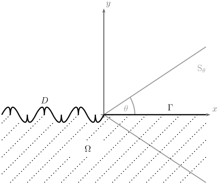
Figure 1. A generic picture of a domain described in Example 3.5.

To verify that such a domain fulfills the geometric setup described in Assumption 2.1, consider first the set

$$\Delta_{\theta}\coloneqq(\mathbb{R}^{2}\setminus\overline{{\mathrm{S}}_{\theta}})\cup\{(x,y)\in\mathbb{R}^{2}:y<0\},$$

which is an $(\varepsilon,\delta)$-domain for some values $\varepsilon,\delta>0$. Since $\Omega\subseteq\Delta_{\theta}$ and $\overline{\Gamma}\subseteq\partial\Delta_{\theta}$, the $(\varepsilon,\delta)$-paths with respect to $\Delta_{\theta}$ for points in $\Omega$ satisfy (LC) and (CC). Hence, to conclude the example, we only have to show that there exists $K>0$ such that for all $z\in\Delta_{\theta}$ and with $\Xi=\mathbb{R}^{2}\setminus\overline{\Gamma}$ it holds

(3.1) $$\operatorname{k}_{\Xi}(\Omega,z)\leq K.$$

Since the paths obtained above take their values only in $\Delta_{\theta}$ this will establish the remaining condition (QHD). Notice that since ${\mathrm{S}}_{\theta}\cap\{(x,y)\in\mathbb{R}^{2}:y<0\}\subseteq\Omega$ it suffices to show that there exists $K>0$ such that for all $z\in\Delta_{\theta}$ it holds

$$\operatorname{k}_{\Xi}({\mathrm{S}}_{\theta}\cap\{(x,y)\in\mathbb{R}^{2}:y<0\},z)\leq K.$$

We only describe one particular case in detail, the remaining cases are similar and left to the interested reader. Assume that $\theta<\pi/2$ and pick $z=(v,w)\in\Delta_{\theta}$ with $v\geq 0$ and $w>0$. Choose $(x,y)\in\partial{\mathrm{S}}_{\theta}$ such that $y\coloneqq-w$ and let $\gamma\coloneqq\gamma_{1}+\gamma_{2}+\gamma_{3}$ with

$$\gamma_{1} :[0,1]\to\mathbb{R}^{2},\quad t\mapsto(x,y)+t(y-x,0),$$

$$\gamma_{2} :[0,1]\to\mathbb{R}^{2},\quad t\mapsto(y,y)+t(0,w-y),$$

$$\gamma_{3} :[0,1]\to\mathbb{R}^{2},\quad t\mapsto(y,w)+t(v-y,0).$$

This construction is depicted in Figure 2.

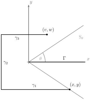
Figure 2. A path connecting $(v,w)$ and $(x,y)$ that is ’short’ with respect to the quasihyperbolic distance.

The path $\gamma$ then connects $(x,y)$ to $(v,w)$ and

$$\operatorname{k}_{\Xi}((x,y),(v,w))\leq\int_{0}^{1}\frac{\lvert y-x\rvert}{\lvert y\rvert}\;\mathrm{d}t+\int_{0}^{1}\frac{\lvert w-y\rvert}{\lvert y\rvert}\;\mathrm{d}t+\int_{0}^{1}\frac{\lvert v-y\rvert}{w}\;\mathrm{d}t=4+\frac{x+v}{w}.$$

Notice that $x=w/\tan(\theta)$ and that $v\leq w/\tan(\theta)$, so that

$$\operatorname{k}_{\Xi}((x,y),(v,w))\leq 2\Big{(}2+\frac{1}{\tan(\theta)}\Big{)}.$$

In the remaining cases $v<0$ and $w\geq 0$, $v<0$ and $w<0$, or $v\geq 0$ and $w<0$ the quasihyperbolic distance to $\Omega$ will even be smaller. This proves the validity of (3.1) and thus, since $\Omega$ is connected and hence (DC) is void, that $\Omega$ fulfills Assumption 2.1.

Remark 3.6.

Notice that the geometric setup in Assumption 3.1 imposes boundary regularity in a neighborhood of $\overline{\Gamma}$, while in the situation described in Example 3.5 the portion $D$ of $\partial\Omega$ can be arbitrarily irregular as long as it stays outside of ${\mathrm{S}}_{\theta}$.

We conclude this section by giving examples of domains where the boundary portion $D$ fails to remain outside of a sector ${\mathrm{S}}_{\theta}$ and show that the $\mathrm{W}^{1,p}_{D}$-extension property fails for these types of domains. These examples show that interior cusps that lie directly on the interface separating $D$ and $\Gamma$ destroy the $\mathrm{W}^{1,p}_{D}$-extension property. The same happens with “interior cusps at infinity”, that is to say, if $D$ and $\Gamma$ approach each other at infinity at a certain rate.

Example 3.7 (Interior boundary cusp in zero).

Let $\alpha\in(1,\infty)$ and consider

$$\Omega\coloneqq\mathbb{R}^{2}\setminus\{(x,y)\in\mathbb{R}^{2}\colon x\geq 0\text{ and }-x^{\alpha}\leq y\leq 0\}.$$

Define $D$ and $\Gamma$ via

$$D\coloneqq\{(x,y)\in\mathbb{R}^{2}:x\geq 0\text{ and }-x^{\alpha}=y\}\qquad\text{and}\qquad\Gamma\coloneqq(0,\infty)\times\{0\}.$$

To prove that the $\mathrm{W}^{1,p}_{D}$-extension property fails, let $1<p<\infty$ and $0<r<\infty$. Let $f_{r}$ be a smooth function, that is supported in

$$Q_{r}\coloneqq\{(x,y)\in\mathbb{R}^{2}:r/2\leq x\leq 2r\text{ and }0\leq y\leq r\},$$

satisfies $0\leq f_{r}\leq 1$, and is identically 1 on

$$R_{r}\coloneqq\{(x,y)\in\mathbb{R}^{2}:3r/4\leq x\leq 3r/2\text{ and }0\leq y\leq r/2\}.$$

Moreover, let $f_{r}$ be such that $\|\nabla f_{r}\|_{\mathrm{L}^{\infty}}\lesssim r^{-1}$. In this case

(3.2) $$\|f_{r}\|_{\mathrm{W}^{1,p}(\Omega)}^{p}\lesssim(r^{2}+r^{2-p}).$$

Next, employ the fundamental theorem of calculus and a density argument to conclude that for all $F\in\mathrm{W}^{1,p}(\mathbb{R}^{d})$ it holds

$$\int_{3r/4}^{3r/2}F(x,0)\;\mathrm{d}x-\int_{3r/4}^{3r/2}F(x,-x^{\alpha})\;\mathrm{d}x=\int_{3r/4}^{3r/2}\int_{-x^{\alpha}}^{0}\partial_{y}F(x,y)\;\mathrm{d}y\;\mathrm{d}x.$$

If there exists a bounded extension operator $E:\mathrm{W}^{1,p}_{D}(\Omega)\to\mathrm{W}^{1,p}_{D}(\mathbb{R}^{2})$, put $F\coloneqq Ef_{r}$ and conclude that the second integral on the left-hand side vanishes since $Ef_{r}\in\mathrm{W}^{1,p}_{D}(\mathbb{R}^{2})$. Using further that by construction the trace of $Ef_{r}$ onto the set $(3r/4,3r/2)\times\{0\}$ is identically $1$, one concludes

$$\frac{3r}{4}\leq\int_{\frac{3r}{4}}^{\frac{3r}{2}}\int_{-x^{\alpha}}^{0}\lvert\partial_{y}Ef_{r}(x,y)\rvert\;\mathrm{d}y\;\mathrm{d}x\lesssim r^{(\alpha+1)/p^{\prime}}\|Ef_{r}\|_{\mathrm{W}^{1,p}(\mathbb{R}^{2})}.$$

Here, $p^{\prime}$ denotes the Hölder-conjugate exponent to $p$. Dividing by $r$ and using that $E$ is bounded delivers together with (3.2) the relation

(3.3) $$1\lesssim r^{(\alpha+1)/p^{\prime}-1}(r^{2/p}+r^{2/p-1}),$$

which results for $r\to 0$ in the condition

$$\frac{\alpha+1}{p^{\prime}}+\frac{2}{p}-2\leq 0\qquad\Longleftrightarrow\qquad\alpha\leq 1.$$

This is a contradiction since $\alpha$ is assumed to be in $(1,\infty)$. Thus, there cannot be a bounded extension operator $E:\mathrm{W}^{1,p}_{D}(\Omega)\to\mathrm{W}^{1,p}_{D}(\mathbb{R}^{2})$.

Example 3.8 (Interior boundary cusp at infinity).

Let $\alpha\in(0,\infty)$ and consider

$$\Omega\coloneqq\{(x,y)\in\mathbb{R}^{2}:\text{either }y>0\text{ or }x>0\text{ and }y<-x^{-\alpha}\}.$$

Define $D$ and $\Gamma$ via

$$D\coloneqq\{(x,y)\in\mathbb{R}^{2}:x>0\text{ and }-x^{-\alpha}=y\}\qquad\text{and}\qquad\Gamma\coloneqq\mathbb{R}\times\{0\}.$$

The proof that in this situation there does not exists a bounded extension operator $E$ from $\mathrm{W}^{1,p}_{D}(\Omega)$ to $\mathrm{W}^{1,p}_{D}(\mathbb{R}^{2})$ for any $p\in(1,\infty)$ is similar to Example 3.7 and we omit the details.

4. Whitney decompositions and the quasihyperbolic distance

In this section, we introduce the Whitney decomposition of an open subset of $\mathbb{R}^{d}$ and show how condition (QHD) relates to properties of Whitney cubes. A cube $Q\subseteq\mathbb{R}^{d}$ is always closed and is said to be dyadic if there exists $k\in\mathbb{Z}$ such that $Q$ coincides with a cube of the mesh determined by the lattice $2^{-k}\mathbb{Z}^{d}$. Two cubes are said to touch if a face of one cube lies in a face of the other cube, and they are said to intersect if their intersection is non-empty. The sidelength of a cube is denoted by $\ell(Q)$. For a number $\alpha>0$ the dilation of $Q$ about its center by the factor $\alpha$ is denoted by $\alpha Q$.

Let $F\subseteq\mathbb{R}^{d}$ be a non-empty closed set. Then, by [22, Thm. VI.1] there exists a collection of cubes $\{Q_{j}\}_{j\in\mathbb{N}}$ with pairwise disjoint interiors such that

1. $\bigcup_{j\in\mathbb{N}}Q_{j}=\mathbb{R}^{d}\setminus F$,

2. $\operatorname{diam}(Q_{j})\leq\operatorname{d}(Q_{j},F)\leq 4\operatorname{diam}(Q_{j})$ for all $j\in\mathbb{N}$,

3. the cubes $\{Q_{j}\}_{j\in\mathbb{N}}$ are dyadic,

4. $\frac{1}{4}\operatorname{diam}(Q_{j})\leq\operatorname{diam}(Q_{k})\leq 4\operatorname{diam}(Q_{j})$ if $Q_{j}\cap Q_{k}\neq\emptyset$,

5. each cube has at most $12^{d}$ intersecting cubes.

The collection $\{Q_{j}\}_{j\in\mathbb{N}}$ are called Whitney cubes and will be denoted by $\mathcal{W}(F)$. In connection with Whitney cubes, the letters (i)-(v) refer always to the above properties. We say that a collection of cubes $Q_{1},\dots,Q_{m}\in\mathcal{W}(F)$ is a touching chain if $Q_{j}$ and $Q_{j+1}$ are touching cubes and that it is an intersecting chain if $Q_{j}\cap Q_{j+1}\neq\emptyset$ for all $j=1,\dots,m-1$. The length of a chain is the number $m$.

Let us mention that for a cube $Q\in\mathcal{W}(F)$ and $x\in Q$ we have $\operatorname{diam}(Q)\geq\frac{1}{5}\operatorname{d}(x,F)$. This follows from

$$4\operatorname{diam}(Q)\geq\operatorname{d}(Q,F)\geq\operatorname{d}(x,F)-\operatorname{diam}(Q),$$

and will be used freely in the rest of this article.

The following lemma translates (QHD) to the existence of intersecting chains of uniformly bounded length. Notice that if $(\Xi_{m})_{m\in\mathcal{I}}$ denotes the connected components of the set $\Xi=\mathbb{R}^{d}\setminus\overline{\Gamma}$, Gehring and Osgood [15, Lem. 1] proved that for any two points $x,y\in\Xi_{m}$ there exists a quasihyperbolic geodesic $\gamma_{x,y}$ with endpoints $x$ and $y$ satisfying

$$\operatorname{k}_{\Xi}(x,y)=\int_{\gamma_{x,y}}\frac{1}{\operatorname{d}(z,\partial\Xi)}\;\lvert\mathrm{d}z\rvert.$$

Trivially, if $\Xi=\mathbb{R}^{d}$, then any path connecting $x$ and $y$ is a quasihyperbolic geodesic.

Lemma 4.1.

Fix $k>0$. There exists a constant $N=N(d,k)\in\mathbb{N}$ such that for all $x,y\in\Xi$ with $\operatorname{k}_{\Xi}(x,y)\leq k$ there exists an intersecting chain $Q_{1},\dots,Q_{m}\in\mathcal{W}(\overline{\Gamma})$ with $x\in Q_{1}$ and $y\in Q_{m}$ and $m\leq N$.

Conversely, if for $x,y\in\Xi$ there exists an intersecting chain connecting $x$ and $y$ of length less than $N\in\mathbb{N}$, then there exists a constant $k=k(N)>0$ such that $\operatorname{k}_{\Xi}(x,y)\leq k$.

Proof.

Notice that $\operatorname{k}_{\Xi}(x,y)<\infty$ implies that $x$ and $y$ lie in the same connected component of $\Xi$. Assume first that

(4.1) $$\lvert x-y\rvert\leq\frac{1}{10\sqrt{d}}\min\{\operatorname{d}(x,\Gamma),\operatorname{d}(y,\Gamma)\}.$$

Let $Q_{x},Q_{y}\in\mathcal{W}(\overline{\Gamma})$ with $x\in Q_{x}$ and $y\in Q_{y}$, and let $\widetilde{Q}_{x}$ denote the region occupied by $Q_{x}$ and all its intersecting Whitney cubes and similarly let $\widetilde{Q}_{y}$ denote its counterpart for $Q_{y}$. Then by (iv)

$$\operatorname{d}(x,\widetilde{Q}_{x}^{c})\geq\frac{1}{4\sqrt{d}}\operatorname{diam}(Q_{x})\qquad\text{and}\qquad\operatorname{d}(y,\widetilde{Q}_{y}^{c})\geq\frac{1}{4\sqrt{d}}\operatorname{diam}(Q_{y}).$$

This combined with (4.1) yields

$$\operatorname{d}(x,\widetilde{Q}_{x}^{c})\geq\frac{1}{4\sqrt{d}}\operatorname{diam}(Q_{x})\geq\frac{1}{2}\lvert x-y\rvert.$$

By symmetry, the same is valid for $y$ instead of $x$. Consequently, $\widetilde{Q}_{x}$ and $\widetilde{Q}_{y}$ have a common point and thus, $x$ and $y$ can be connected by an intersecting chain of length at most $4$.

Now, let

$$\lvert x-y\rvert>\frac{1}{10\sqrt{d}}\min\{\operatorname{d}(x,\Gamma),\operatorname{d}(y,\Gamma)\}.$$

Assume without loss of generality that $\operatorname{d}(x,\Gamma)\leq\operatorname{d}(y,\Gamma)$. Fix a quasihyperbolic geodesic $\gamma_{x,y}$ that connects $x$ with $y$ (see the discussion before this proof). Then Herron and Koskela [19, Prop. 2.2] ensures the existence of points $y_{0}\coloneqq x,y_{1},\dots,y_{\ell}\in\mathbb{R}^{d}\setminus\overline{\Gamma}$ such that $\gamma_{x,y}$ is contained in the closure of $\bigcup_{i=0}^{\ell}B_{i}$, where $B_{i}\coloneqq\mathrm{B}(y_{i},r_{i})$ with $r_{i}\coloneqq\operatorname{d}(y_{i},\Gamma)/(10\sqrt{d})$, and such that

(4.2) $$\ell\leq 20\sqrt{d}\operatorname{k}_{\Xi}(x,y).$$

Next, we estimate the number of Whitney cubes that cover each of these balls. Denote the number of Whitney cubes that cover $\overline{B_{i}}$ by $W_{i}$. Let $Q\in\mathcal{W}(\overline{\Gamma})$ be such that $Q\cap\overline{B_{i}}\neq\emptyset$. Then,

$$\operatorname{diam}(Q)\geq\frac{1}{4}\operatorname{d}(Q,\Gamma)\geq\frac{1}{4}[\operatorname{d}(y_{i},\Gamma)-r_{i}-\operatorname{diam}(Q)],$$

so that by definition of $r_{i}$

$$\operatorname{diam}(Q)\geq\frac{(10\sqrt{d}-1)\operatorname{d}(y_{i},\Gamma)}{50\sqrt{d}}.$$

Moreover,

$$\operatorname{diam}(Q) \leq\operatorname{d}(Q,\Gamma)\leq\operatorname{d}(B_{i}\cap Q,\Gamma)\leq\operatorname{d}(y_{i},\Gamma)+r_{i}=\bigg{[}1+\frac{1}{10\sqrt{d}}\bigg{]}\operatorname{d}(y_{i},\Gamma).$$

Consequently,

$$W_{i}\bigg{[}\frac{(10\sqrt{d}-1)\operatorname{d}(y_{i},\Gamma)}{50d}\bigg{]}^{d} \leq\sum_{\begin{subarray}{c}Q\in\mathcal{W}(\overline{\Gamma})\\ Q\cap\overline{B_{i}}\neq\emptyset\end{subarray}}\lvert Q\rvert\leq\Big{\lvert}B\Big{(}y_{i},\Big{[}1+\frac{1}{5\sqrt{d}}\Big{]}\operatorname{d}(y_{i},\Gamma)\Big{)}\Big{\rvert},$$

what proves that $W_{i}$ is controlled by a constant depending only on $d$. We conclude by (4.2) and by the bound on each $W_{i}$ that there exists an intersecting chain connecting $x$ and $y$ of length bounded by a constant depending only on $d$ and $k$.

For the other direction, let $Q_{1},\dots,Q_{m}$ be an intersecting chain that connects $x$ with $y$ and with $m\leq N$. Thus, by definition $Q_{j}\cap Q_{j+1}\neq\emptyset$. Let $\gamma$ be a path connecting $x$ and $y$ which is constructed by linearly connecting a point in $Q_{j-1}\cap Q_{j}$ with a point in $Q_{j}\cap Q_{j+1}$. Thus, employing (ii) delivers

$$\operatorname{k}_{\Xi}(x,y) \leq\sum_{j=1}^{m}\int_{\gamma\cap Q_{j}}\frac{1}{\operatorname{d}(Q_{j},\Gamma)}\;\lvert\mathrm{d}z\rvert\leq\sum_{j=1}^{m}\frac{\operatorname{diam}(Q_{j})}{\operatorname{diam}(Q_{j})}=m.\qed$$

5. Cubes and chains

In this section, we describe how to ’reflect’ cubes at $\overline{\Gamma}$ if $\Omega$ is subject to Assumption 2.1 and establish some natural properties of theses ’reflections’. This is an adaption of an argument of Jones presented in [20]. Throughout, assume in Sections 5 and 6 that $\Omega$ is an open set subject to Assumption 2.1 which satisfies $\overline{\Omega}\neq\mathbb{R}^{d}$. (When $\Omega$ is dense in $\mathbb{R}^{d}$, Theorem 1.2 follows in a trivial way. The details will be presented separately in the proof of the theorem). Recall that we assume $\operatorname{diam}(\Omega_{m})\geq\lambda\delta$, where $(\Omega_{m})_{m}$ are the connected components of $\Omega$ whose boundary hits $\Gamma$. This is in contrast to [20] where Jones assumes without loss of generality (by scaling) that the domain has radius at least $1$ and that $\delta$ is at most $1$. However, this has the disadvantage that homogeneous estimates will only be achievable on small scales even if $\delta=\infty$ and the domain is unbounded. We will comment on this topic later on in Remark 6.11.

Lemma 5.1.

We have $\lvert\Gamma\rvert=0$.

Proof.

Fix $x_{0}\in\Gamma$ and $y\in\Omega$ with $\lvert x_{0}-y\rvert<\frac{\delta}{2}$. Let $Q$ be any cube in $\mathbb{R}^{d}$ centered in $x_{0}$ with $l(Q)\leq\frac{1}{2}\lvert x_{0}-y\rvert$. We will show that $[\mathbb{R}^{d}\setminus\Gamma]\cap Q$ has Lebesgue measure comparable to that of $Q$. Let $x\in\Omega$ with $\lvert x-x_{0}\rvert\leq\frac{1}{8}l(Q)$. Then, we have

(5.1) $$\lvert x-y\rvert\geq\frac{15}{8}l(Q)\qquad\text{and}\qquad\lvert x-y\rvert\leq\frac{17}{16}\lvert x_{0}-y\rvert.$$

Let $\gamma$ be a path connecting $x$ and $y$ subject to Assumption 2.1 (note that $|x-y|<\delta$ is either void if $\delta=\infty$ or otherwise it follows from the second inequality in (5.1)). By virtue of (5.1), the intermediate value theorem implies that there exists $z\in\gamma$ with $\lvert x-z\rvert=\frac{1}{8}l(Q)$. This point lies in $\frac{1}{2}Q$ by construction. Moreover, (CC) together with $\lvert y-z\rvert\geq\lvert x-y\rvert-\lvert x-z\rvert$ implies

$$\operatorname{d}(z,\Gamma)\geq\frac{\varepsilon l(Q)}{8}\frac{\lvert x-y\rvert-\lvert x-z\rvert}{\lvert x-y\rvert}\geq\frac{\varepsilon l(Q)}{8}(1-\frac{l(Q)}{8|x-y|})\geq\frac{7\varepsilon}{60}l(Q).$$

Thus, $\limsup_{l(Q)\to 0}\frac{\lvert[\mathbb{R}^{d}\setminus\Gamma]\cap Q\rvert}{\lvert Q\rvert}>0$, where the $\limsup$ is taken over all cubes centered at $x_{0}$. Since $\chi_{\mathbb{R}^{d}\setminus\Gamma}(x_{0})=0$ and $\chi_{\mathbb{R}^{d}\setminus\Gamma}\in\mathrm{L}^{1}_{\mathrm{loc}}(\mathbb{R}^{d})$ Lebesgue’s differentiation theorem implies $\lvert\Gamma\rvert=0$. ∎

To proceed, we define two families of cubes. The family of interior cubes is given by

$$\mathcal{W}_{i}\coloneqq\{Q\in\mathcal{W}(\overline{\Gamma}):Q\cap\Omega\neq\emptyset\}.$$

These interior cubes will be the reflections of exterior cubes $\mathcal{W}_{e}$. To define $\mathcal{W}_{e}$ we use numbers $A>0$ and $B>2$ whose values are to be fixed during this section and define

$$\mathcal{W}_{e}\coloneqq\{Q\in\mathcal{W}(\overline{\Omega}):\operatorname{diam}(Q)\leq A\delta\text{ and }\operatorname{d}(Q,\Gamma)<B\operatorname{d}(Q,\partial\Omega\setminus\Gamma)\}.$$

Remark 5.2.

First, the collection $\mathcal{W}_{e}$ is empty if and only if $D=\partial\Omega$. Indeed, if $D=\partial\Omega$ then the second condition in the definition $\mathcal{W}_{e}$ can never be fulfilled. To the contrary, if $\Gamma$ is non-empty, then, using the relative openness of $\Gamma$, one can fix a ball centered in $\Gamma$ that does not intersect $D$, and small cubes inside this ball will satisfy both conditions. Second, if $D\neq\partial\Omega$, then for a cube $Q\in\mathcal{W}_{e}$ we have

$$\operatorname{d}(Q,\Omega)=\min\{\operatorname{d}(Q,\Gamma),\operatorname{d}(Q,\partial\Omega\setminus\Gamma)\}\geq B^{-1}\operatorname{d}(Q,\Gamma)$$

what implies that for all $Q\in\mathcal{W}_{e}$ it holds

(5.2) $$\operatorname{d}(Q,\Omega)\leq\operatorname{d}(Q,\Gamma)\leq B\operatorname{d}(Q,\Omega).$$

Thus, the diameter of $Q$ is comparable to its distance to $\Gamma$.

For the rest of this section, we assume that $\Gamma\neq\emptyset$. Before we present how to ’reflect’ cubes, we prove a technical lemma that, given an exterior cube $Q\in\mathcal{W}_{e}$, allows us to find a connected component of $\Omega$ whose boundary intersects $\Gamma$ and which is not too far away from $Q$.

Lemma 5.3.

Let $Q\in\mathcal{W}_{e}$. Then there exists a connected component $\Omega_{m}$ of $\Omega$ with $\Gamma\cap\partial\Omega_{m}\neq\emptyset$ and $x\in\Omega_{m}$ with

$$\operatorname{d}(x,Q)\leq 5B\operatorname{diam}(Q).$$

Proof.

By (ii) and Remark 5.2, there exists $x^{\prime}\in\overline{\Gamma}$ such that $\operatorname{d}(x^{\prime},Q)\leq 4B\operatorname{diam}(Q)$. Since $x^{\prime}\in\overline{\Gamma}$ there is $x^{\prime\prime}\in\Gamma$ with $\operatorname{d}(x^{\prime\prime},Q)\leq\frac{9}{2}B\operatorname{diam}(Q)$.

Denote the at most countable family of connected components of $\Omega$ whose boundary has a non-empty intersection with $\Gamma$ by $\{\Omega_{m}\}_{m}$ and the connected components whose boundary has an empty intersection with $\Gamma$ by $\{\Upsilon_{m}\}_{m}$.

If there is $\Omega_{m}$ with $x^{\prime\prime}\in\partial\Omega_{m}$, then the proof is finished. If not, pick a sequence $(x_{n})_{n}$ in $\Omega$ that converges to $x^{\prime\prime}\in\Gamma\subseteq\partial\Omega$. If almost all $x_{n}$ are contained in the union of the $\Omega_{m}$, this concludes the proof as well. Otherwise, choose a subsequence (again denoted by $x_{n}$) for which there are indices $m_{n}$ such that $x_{n}\in\Upsilon_{m_{n}}$. Furthermore, $x^{\prime\prime}\in\overline{\Upsilon}_{m}^{c}$ for all $m$ since $\Gamma\cap\partial\Upsilon_{m}=\emptyset$. Now, by connecting $x^{\prime\prime}$ and $x_{n}$ by a straight line, the intermediate value theorem implies the existence of a point $x_{n}^{\prime}\in\partial\Upsilon_{m_{n}}$ with

$$\lvert x^{\prime\prime}-x_{n}^{\prime}\rvert\leq\lvert x^{\prime\prime}-x_{n}\rvert.$$

Passing to the limit $n\to\infty$ yields $x^{\prime\prime}\in D$ by the closedness of $D$ and thus a contradiction. ∎

The following lemma assigns to every cube in $\mathcal{W}_{e}$ a ‘reflected’ cube in $\mathcal{W}_{i}$. For the rest of Sections 5 and 6 we will reserve the letter $N$ to denote the constant $N$ appearing in Lemma 4.1 applied with $k=2K$, where $K$ is the number from Assumption 2.1. Notice that $N$ solely depends on $d$ and $K$. For the rest of this paper we make the following agreement.

Agreement 1.

If $X$ and $Y$ are two quantities and if there exists a constant $C$ depending only on $d$, $p$, $K$, $\lambda$, and $\varepsilon$ such that $X\leq CY$ holds, then we will write $X\lesssim Y$ or $Y\gtrsim X$. If both $\frac{Y}{C}\leq X\leq CY$ holds, then we will write $X\simeq Y$.

Lemma 5.4.

There exist constants $C_{1}=C_{1}(N,\varepsilon)>0$ and $C_{2}=C_{2}(\lambda)>0$ such that if $AB\leq C_{1}$ and $B\geq C_{2}$, then for every $Q\in\mathcal{W}_{e}$ there exists a cube $R\in\mathcal{W}_{i}$ satisfying

(5.3) $$\operatorname{diam}(Q)\leq\operatorname{diam}(R)\lesssim(1+B+(AB)^{-1})\operatorname{diam}(Q)$$

and

(5.4) $$\operatorname{d}(R,Q)\lesssim(1+B+(AB)^{-1})\operatorname{diam}(Q).$$

Proof.

Fix $Q\in\mathcal{W}_{e}$ and recall that $\operatorname{diam}(Q)\leq A\delta$ by definition of $\mathcal{W}_{e}$ and $B>2$. By Lemma 5.3 there exists a connected component $\Omega_{m}$ of $\Omega$ with $\Gamma\cap\partial\Omega_{m}\neq\emptyset$ and $x\in\Omega_{m}$ with $\operatorname{d}(x,Q)\leq 5B\operatorname{diam}(Q)$. We introduce the additional lower bound $B\geq 3/\lambda$, which is only needed in the case $\delta<\infty$ but we choose $B$ always that large for good measure.

So, in the case $\delta<\infty$, since $(AB)^{-1}\operatorname{diam}(Q)\leq\delta B^{-1}<\min(\delta,\lambda\delta/2)\leq\min(\delta,\,\operatorname{diam}(\Omega_{m})/2)$ according to (DC), we find $y\in\Omega_{m}$ satisfying

(5.5) $$\lvert x-y\rvert=(AB)^{-1}\operatorname{diam}(Q)\qquad\text{and}\qquad\lvert x-y\rvert<\delta.$$

If $\delta=\infty$, then $\Omega$ is unbounded, so we again find $y\in\Omega$ satisfying the first condition whereas the second becomes void for Assumption 2.1.

Hence, let $\gamma$ be a path provided by Assumption 2.1 connecting $x$ and $y$, and let $z\in\gamma$ with $\lvert x-z\rvert=\frac{1}{2}\lvert x-y\rvert$. Estimate by virtue of (CC) and (5.5)

(5.6) $$\operatorname{d}(z,\Gamma)\geq\frac{\varepsilon}{2}\lvert y-z\rvert\geq\frac{\varepsilon}{2}\big{(}\lvert x-y\rvert-\lvert x-z\rvert\big{)}=\frac{\varepsilon}{4}(AB)^{-1}\operatorname{diam}(Q).$$

By Assumption 2.1 we have $\operatorname{k}_{\Xi}(z,\Omega)\leq K$, hence there exists $z^{\prime}\in\Omega$ with $\operatorname{k}_{\Xi}(z,z^{\prime})\leq 2K$. Thus, by Lemma 4.1 there exists an intersecting chain $Q_{1},\dots,Q_{m}\in\mathcal{W}(\overline{\Gamma})$ with $Q_{m}\cap\Omega\neq\emptyset$, $z\in Q_{1}$, and $m\leq N$. Choose the reflected cube as $R\coloneqq Q_{m}$. Using (ii) and (iv) one gets

$$4\operatorname{diam}(R)\geq\operatorname{d}(R,\Gamma)\geq\operatorname{d}(z,\Gamma)-\sum_{j=1}^{m}\operatorname{diam}(Q_{j})\geq\operatorname{d}(z,\Gamma)-\sum_{j=1}^{m}4^{m-j}\operatorname{diam}(R).$$

Thus, by (5.6) and $m\leq N$

$$\frac{11+4^{N}}{3}\operatorname{diam}(R)\geq\frac{\varepsilon}{4}(AB)^{-1}\operatorname{diam}(Q).$$

Consequently, there exists $C=C(N,\varepsilon)>0$ such that $AB\leq C$ implies $\operatorname{diam}(Q)\leq\operatorname{diam}(R)$.

In order to control $\operatorname{diam}(R)$ by $\operatorname{diam}(Q)$, employ (ii), (iv), and the triangle inequality to deduce

$$4^{1-m}\operatorname{diam}(R)\leq\operatorname{diam}(Q_{1})\leq\operatorname{d}(z,\Gamma)\leq\operatorname{d}(z,Q)+\operatorname{diam}(Q)+\operatorname{d}(Q,\Gamma).$$

The right-hand side is estimated by the triangle inequality, followed by (5.2) and (ii), the choice $\lvert x-z\rvert=\frac{1}{2}\lvert x-y\rvert$ combined with (5.5), and $\operatorname{d}(x,Q)\leq 5B\operatorname{diam}(Q)$, yielding

$$\operatorname{d}(z,Q)+\operatorname{diam}(Q)+\operatorname{d}(Q,\Gamma) \leq\lvert z-x\rvert+\operatorname{d}(x,Q)+\operatorname{diam}(Q)+B\operatorname{d}(Q,\Omega)$$

$$\leq((2AB)^{-1}+1+9B)\operatorname{diam}(Q).$$

Taking into account that $\operatorname{d}(z,R)\leq\operatorname{diam}(R)(4^{m}-1)/3$ (estimate the sizes of the cubes in the connecting chain using a geometric sum), the distance from $R$ to $Q$ is estimated similarly, yielding

$$\operatorname{d}(R,Q) \leq\operatorname{diam}(R)+\operatorname{diam}(Q)+\lvert x-z\rvert+\operatorname{d}(z,R)+\operatorname{d}(x,Q)$$

$$\leq(1+(2AB)^{-1}+5B)\operatorname{diam}(Q)+\frac{4^{m}+2}{3}\operatorname{diam}(R).$$

Together with the previous estimate, this concludes the proof. ∎

For the rest of this article, we fix the notation that if $Q\in\mathcal{W}_{e}$ and $R\in\mathcal{W}_{i}$ is the cube constructed in Lemma 5.4, then $R$ is denoted by $R=Q^{*}$ and $Q^{*}$ is called the reflected cube of $Q$. The next lemma gives a bound on the distance of reflected cubes of two intersecting cubes. Its proof is a direct consequence of Lemma 5.4 and (iv), and is thus omitted.

Lemma 5.5.

If $Q_{1},Q_{2}\in\mathcal{W}_{e}$ with $Q_{1}\cap Q_{2}\neq\emptyset$, then

$$\operatorname{d}(Q_{1}^{*},Q_{2}^{*})\lesssim(1+B+(AB)^{-1})\operatorname{diam}(Q_{1}).$$

In the proof of the boundedness of the extension operator, one needs to connect Whitney cubes by appropriate touching chains. The following lemma presents a basic principle of how to build a chain out of a path $\gamma$ and how the quantities $\mathrm{length}(\gamma)$ and $\operatorname{d}(\gamma,\Gamma)$ translate into the length of the chain and the distance of the cubes of the chain to $\Gamma$.

Lemma 5.6.

Let $R_{1},R_{2}\in\mathcal{W}(\overline{\Gamma})$ with $R_{1}\neq R_{2}$ and let $x\in R_{1}$, $y\in R_{2}$, and $\gamma$ be a rectifiable path in $\mathbb{R}^{d}\setminus\overline{\Gamma}$ connecting $x$ and $y$. Assume that there exist constants $C_{1},C_{2}>0$ such that $\mathrm{length}(\gamma)\leq C_{1}\operatorname{diam}(R_{1})$ and $\operatorname{d}(z,\Gamma)\geq C_{2}\operatorname{diam}(R_{1})$ for all $z\in\gamma$, then there exists a touching chain of cubes $R_{1}=S_{1},\dots,S_{m}=R_{2}$ in $\mathcal{W}(\overline{\Gamma})$, where $m$ is bounded by a number depending only on $d$, $C_{1}$, and $C_{2}$. Moreover,

$$\frac{C_{2}}{5}\operatorname{diam}(R_{1})\leq\operatorname{diam}(S_{i})\leq(5+C_{1})\operatorname{diam}(R_{1})\qquad(i=1,\dots,m).$$

Proof.

Let $\mathcal{S}$ be the finite set of cubes in $\mathcal{W}(\overline{\Gamma})$ intersecting $\gamma$. For $S\in\mathcal{S}$ one finds by (ii) and by assumption that $\operatorname{diam}(S)\geq\frac{C_{2}}{5}\operatorname{diam}(R_{1})$. Fix $z\in S\cap\gamma$, then

$$\operatorname{d}(z,\Gamma)\leq\operatorname{d}(x,\Gamma)+\lvert x-z\rvert\leq 5\operatorname{diam}(R_{1})+\mathrm{length}(\gamma)\leq(5+C_{1})\operatorname{diam}(R_{1}),$$

so that $\operatorname{diam}(S)\leq(5+C_{1})\operatorname{diam}(R_{1})$ by (ii). This, together with $\mathrm{length}(\gamma)\leq C_{1}\operatorname{diam}(R_{1})$ implies that $S\subseteq\mathrm{B}(x,(5+2C_{1})\operatorname{diam}(R_{1}))$. Because all elements of $\mathcal{S}$ are mutually disjoint one finds

$$\sharp(\mathcal{S})\leq\frac{\lvert\mathrm{B}(x,(5+2C_{1})\operatorname{diam}(R_{1}))\rvert}{(\frac{C_{2}}{5\sqrt{d}}\operatorname{diam}(R_{1}))^{d}}=\omega_{d}\bigg{(}\frac{5\sqrt{d}(5+2C_{1})}{C_{2}}\bigg{)}^{d},$$

where $\sharp(\mathcal{S})$ denotes the cardinality of $\mathcal{S}$ and $\omega_{d}\coloneqq\lvert\mathrm{B}(0,1)\rvert$. By (iii) the elements of $\mathcal{S}$ are dyadic and thus one finds a subset of $\mathcal{S}$ which is a touching chain starting at $R_{1}$ and ending at $R_{2}$. ∎

Lemma 5.7.

There exist constants $C_{1},C_{2}>0$ depending only on $\varepsilon$, $d$, $\lambda$, and $K$ such that if $A\leq C_{1}$ and $B\geq C_{2}$ and if $Q_{j},Q_{k}\in\mathcal{W}_{e}$ with $Q_{j}\cap Q_{k}\neq\emptyset$, then there exists a touching chain $F_{j,k}=\{Q_{j}^{*}=S_{1},\dots,S_{m}=Q_{k}^{*}\}$ of cubes in $\mathcal{W}(\overline{\Gamma})$ connecting $Q_{j}^{*}$ and $Q_{k}^{*}$, where $m$ can be bounded uniformly by a constant depending only on $\varepsilon$, $d$, $K$, $A$, and $B$. Moreover, there exist $K_{1},K_{2}>0$ depending only on $\varepsilon$, $d$, $K$, $A$, and $B$ such that

$$K_{1}\operatorname{diam}(Q_{j})\leq\operatorname{diam}(S_{i})\leq K_{2}\operatorname{diam}(Q_{j})\qquad(i=1,\dots,m).$$

Proof.

If $Q_{j}^{*}=Q_{k}^{*}$ there is nothing to show. Thus, assume $Q_{j}^{*}\neq Q_{k}^{*}$ and let $x\in Q_{j}^{\ast}$ and $y\in Q_{k}^{\ast}$. We show in the following that the assumptions of Lemma 5.6 are satisfied.

Using Lemmas 5.4 and 5.5 in conjunction with (iv) gives

(5.7) $$\lvert x-y\rvert\leq\operatorname{d}(Q_{j}^{*},Q_{k}^{*})+\operatorname{diam}(Q_{j}^{*})+\operatorname{diam}(Q_{k}^{*})\lesssim(1+B+(AB)^{-1})\operatorname{diam}(Q_{j}).$$

If $\delta$ is finite we get, since $Q_{j}\in\mathcal{W}_{e}$, that

$$|x-y|\lesssim(A+AB+B^{-1})\delta,$$

so we obtain $|x-y|<\delta$ when we first choose $B$ large enough and afterwards $A$ sufficiently small. Let $\gamma$ be a path connecting $x$ and $y$ according to Assumption 2.1. By (LC), (5.7), and (5.3) one finds

$$\mathrm{length}(\gamma)\lesssim(1+B+(AB)^{-1})\operatorname{diam}(Q_{j}^{*}).$$

To estimate the distance between each $z\in\gamma$ and $\Gamma$, notice that if $\lvert x-z\rvert\leq\frac{1}{2}\operatorname{diam}(Q_{j}^{*})$, then $\operatorname{d}(z,\Gamma)\geq\frac{1}{2}\operatorname{diam}(Q_{j}^{*})$. Analogously, but by employing additionally (5.3) twice and (iv), if $\lvert y-z\rvert\leq\frac{1}{2}\operatorname{diam}(Q_{k}^{*})$, then

(5.8) $$\operatorname{d}(z,\Gamma)\geq\frac{1}{2}\operatorname{diam}(Q_{k}^{*})\geq\frac{1}{2}\operatorname{diam}(Q_{k})\geq\frac{1}{8}\operatorname{diam}(Q_{j})\gtrsim\big{(}1+B+(AB)^{-1}\big{)}^{-1}\operatorname{diam}(Q_{j}^{*}).$$

In the remaining case, one estimates by (CC), the calculation performed in (5.8), and (5.7) that

$$\operatorname{d}(z,\Gamma) \gtrsim\frac{\operatorname{diam}(Q_{j}^{*})^{2}}{(1+B+(AB)^{-1})\lvert x-y\rvert}\gtrsim\frac{\operatorname{diam}(Q_{j}^{*})}{(1+B+(AB)^{-1})^{2}}.\qed$$

The following lemma provides the existence of chains that ‘escape $\Omega$’ for reflections of cubes $Q\in\mathcal{W}(\overline{\Omega})$ that are close to a relatively open portion of $D$. These chains will be important to obtain a Poincaré inequality with a quantitative control of the constants.

Lemma 5.8.

There exist constants $C_{1},C_{2}>0$ depending only on $\varepsilon$, $d$, $\lambda$, and $K$ such that if $A\leq C_{1}$ and $B\geq C_{2}$ and if $Q\in\mathcal{W}(\overline{\Omega})\setminus\mathcal{W}_{e}$ satisfies $\operatorname{diam}(Q)\leq A\delta$ and has a non-empty intersection with a cube in $\mathcal{W}_{e}$, then for each intersecting cube $Q_{j}\in\mathcal{W}_{e}$ of $Q$, there exists a touching chain $F_{P,j}=\{Q_{j}^{*}=S_{1},\dots,S_{m}\}$ of cubes in $\mathcal{W}(\overline{\Gamma})$, where $m$ is bounded by a constant depending only on $\varepsilon$, $d$, $K$, $A$, and $B$ and $S_{m}\cap Q_{j}$ is a dyadic cube that satisfies

$$\lvert S_{m}\cap Q_{j}\rvert\gtrsim\operatorname{diam}(Q_{j})^{d}.$$

Furthermore, all $S_{i}\in F_{P,j}$ satisfy

$$K_{1}\operatorname{diam}(Q_{j})\leq\operatorname{diam}(S_{i})\leq K_{2}\operatorname{diam}(Q_{j})\qquad(i=1,\dots,m).$$

The constants $K_{1},K_{2}>0$ depend only on $\varepsilon$, $d$, $K$, $A$, and $B$.

Proof.

Let $Q_{j}\in\mathcal{W}_{e}$ be an intersecting cube of $Q$. Then, using properties of the Whitney cubes and $Q\notin\mathcal{W}_{e}$, one estimates

(5.9) $$B\operatorname{d}(Q_{j},\partial\Omega\setminus\Gamma)\leq 6B\operatorname{d}(Q,\partial\Omega\setminus\Gamma)\leq 6\operatorname{d}(Q,\Gamma)\leq 36\operatorname{d}(Q_{j},\Gamma).$$

Let $B\geq 720$, then (5.9) and Remark 5.2 imply $\operatorname{d}(Q_{j},\partial\Omega\setminus\Gamma)=\operatorname{d}(Q_{j},\Omega)$. Hence, using (5.9) again and (iv), one finds that $\operatorname{d}(Q_{j},\Gamma)\geq\frac{B}{36}\operatorname{d}(Q_{j},\Omega)\geq\frac{B}{36}\operatorname{diam}(Q_{j})$. Let $x_{0}\in D$ be such that $\operatorname{d}(x_{0},Q_{j})=\operatorname{d}(Q_{j},\Omega)\leq 4\operatorname{diam}(Q_{j})$. The properties collected above then imply

$$\operatorname{d}(x_{0},\Gamma)\geq\operatorname{d}(Q_{j},\Gamma)-\operatorname{d}(x_{0},Q_{j})-\operatorname{diam}(Q_{j})\geq(36^{-1}B-5)\operatorname{diam}(Q_{j}),$$

and if $y$ is any point from $\mathrm{B}(x_{0},5\operatorname{diam}(Q_{j}))$ then the previous estimate delivers

$$\operatorname{d}(y,\Gamma)\geq\operatorname{d}(x_{0},\Gamma)-5\operatorname{diam}(Q_{j})\geq(36^{-1}B-10)\operatorname{diam}(Q_{j})\geq 10\operatorname{diam}(Q_{j}).$$

Fix $y\in\mathrm{B}(x_{0},5\operatorname{diam}(Q_{j}))\cap\Omega$. Notice that the midpoint $z$ of $Q_{j}$ is contained in $\mathrm{B}(x_{0},5\operatorname{diam}(Q_{j}))$. Thus, each point on the line segment $\gamma_{1}$ connecting $y$ to $z$ has at least a distance which is larger than $10\operatorname{diam}(Q_{j})$ to $\Gamma$.

For $x\in Q_{j}^{*}\cap\Omega$ Lemma 5.4 together with $\{y\}\cup Q_{j}\subseteq\mathrm{B}(x_{0},6\operatorname{diam}(Q_{j}))$ implies

$$\lvert x-y\rvert\leq\operatorname{d}(y,Q_{j})+\operatorname{d}(Q_{j},Q_{j}^{*})+\operatorname{diam}(Q_{j})+\operatorname{diam}(Q_{j}^{*})\lesssim(1+B+(AB)^{-1})\operatorname{diam}(Q_{j}).$$

If $\delta$ is finite, we can ensure $|x-y|<\delta$ using exactly the same argument as in the proof of Lemma 5.7 and otherwise this condition is again meaningless. Let $\gamma_{2}$ be the path connecting $x$ and $y$ subject to Assumption 2.1 and let $Q\in\mathcal{W}(\overline{\Gamma})$ with $y\in Q$. Since $\operatorname{d}(Q,\Gamma)\geq C\operatorname{diam}(Q_{j}^{*})$ for some $C>0$ depending only on $\varepsilon$, $K$, $d$, $A$, and $B$, one concludes as in the proof of Lemma 5.7 that the path $\gamma_{2}$, and hence, by the consideration above, also the path $\gamma=\gamma_{1}+\gamma_{2}$ which connects $x\in Q_{j}^{\ast}$ with $z\in Q_{j}$ satisfies the assumptions of Lemma 5.6, where $Q_{j}^{\ast}$ fulfills the role of $R_{1}$ and $R_{2}$ is some cube in $\mathcal{W}(\overline{\Gamma})$ that contains $z$. Note that the constants appearing in Lemma 5.6 depend only on $\varepsilon$, $K$, $d$, $A$, and $B$.

As in the statement of the lemma we write $S_{m}$ for $R_{2}$ and distinguish cases for the relation between $S_{m}$ and $Q_{j}$. Since $Q_{j}\cap S_{m}\neq\emptyset$ and since Whitney cubes are dyadic, it either holds $S_{m}\subseteq Q_{j}$ or $Q_{j}\subseteq S_{m}$. If $Q_{j}\subseteq S_{m}$ the proof is finished. If $S_{m}\subseteq Q_{j}$, then

$$4\operatorname{diam}(S_{m})\geq\operatorname{d}(S_{m},\Gamma)\geq\operatorname{d}(Q_{j},\Gamma)\geq 36^{-1}B\operatorname{diam}(Q_{j}),$$

so that $\lvert S_{m}\cap Q_{j}\rvert\gtrsim\operatorname{diam}(Q_{j})^{d}$. ∎

The next lemma shows that for a fixed cube $R\in\mathcal{W}_{i}$, there are only finitely many cubes in $\mathcal{W}_{e}$, whose reflected cube is $R$.

Lemma 5.9.

There is a constant $C\in\mathbb{N}$ such that for each $R\in\mathcal{W}_{i}$ there are at most $C$ cubes $Q\in\mathcal{W}_{e}$ such that $Q^{*}=R$, where $C$ solely depends on $d$, $K$, $A$, $B$, and $\varepsilon$.

Proof.

Let $\alpha$ denote the constant from (5.4) and let $Q\in\mathcal{W}_{e}$ with reflected cube $R$, then it follows with (5.3) that $\operatorname{d}(R,Q)\leq\alpha\operatorname{diam}(R)$. So, if $x_{R}$ denotes the center of $R$, every cube $Q$ with $Q^{*}=R$ must be contained in $\mathrm{B}(x_{R},(\alpha+\frac{3}{2})\operatorname{diam}(R))$. Because for those cubes $\operatorname{diam}(Q)$ is controlled from below by $\operatorname{diam}(R)$ according to (5.3) and because cubes from $\mathcal{W}_{e}$ have disjoint interiors, the lemma follows by a counting argument. ∎

6. Construction of the extension operator and exterior estimates

This section is devoted to the construction of the extension operator from Theorem 1.2. We also establish estimates for the operator on $\overline{\Omega}^{c}$. To do so, we start with a preparatory part on (adapted) polynomials, followed by some overlap considerations. We proceed with the construction of the extension operator, in which the adapted polynomials will appear, followed by the exterior estimates, for which we will need the results on overlap.

Agreement 2.

If not otherwise mentioned, the symbols $k$ and $p$ are supposed to refer to these parameters in Theorem 1.2. The numbers $A$ and $B$ which were introduced in Section 5 will be considered as fixed numbers depending only on $\varepsilon$, $d$, $K$, and $\lambda$ such that all statements in Section 5 are valid. From now on we will use the symbols $\lesssim$ and $\gtrsim$ in a more liberal way than described in Agreement 1.

Polynomial fitting and Poincaré type estimates

We record some results on polynomial approximation and Poincaré type estimates. Most of them stem from [6] and where used therein for a similar purpose.

We start out with the following generic norm comparison lemma for polynomials of fixed degree, see [6, Lem. 2.3].

Lemma 6.1.

Let $Q,R$ be cubes with $R\subseteq Q$ and assume that there exists a constant $\kappa>0$ such that $|R|\geq\kappa|Q|$. Then for each polynomial $P$ of degree at most $m$ one has

$$\|P\|_{\mathrm{L}^{p}(Q)}\lesssim\|P\|_{\mathrm{L}^{p}(R)},$$

where the implicit constant does only depend on $d$, $\kappa$, $p$, and $m$. In particular, if $S$ is another cube with $S\subseteq Q$ and $|S|\geq\kappa|Q|$, then the $\mathrm{L}^{p}$ norms over $R$ and $S$ are equivalent norms on $\mathcal{P}_{m}$ and the implicit constants do only depend on $d$, $\kappa$, $p$, and $m$.

The following lemma provides “adapted” polynomials together with corresponding Poincaré type estimates. A proof can be found in [6, Thm. 4.5, Thm. 4.7 & Rem. 4.8], note that the proof of the remark still works when replacing Whitney cubes by cubes of the same size.

Lemma 6.2.

Let $Q$ be a cube, $R$ a touching cube of $Q$ of the same size, and $k\geq 0$ an integer. Then there exists a projection $P:\mathrm{L}^{1}(Q)\to\mathcal{P}_{k-1}$ that satisfies the estimate

(6.1) $$\|\partial^{\alpha}Pf\|_{\mathrm{L}^{p}(Q)}\lesssim\|\partial^{\alpha}f\|_{\mathrm{L}^{p}(Q)}$$

for $f\in\mathrm{C}_{D}^{\infty}(\mathbb{R}^{d})\cap\mathrm{W}^{k,p}(Q)$, $|\alpha|\leq k$ and $1\leq p\leq\infty$. Moreover, the Poincaré type estimate

(6.2) $$\|\partial^{\alpha}(f-Pf)\|_{\mathrm{L}^{p}(Q\cup R)}\lesssim\operatorname{diam}(Q)^{\ell-|\alpha|}\|\nabla^{\ell}f\|_{\mathrm{L}^{p}(Q\cup R)},$$

holds for $f\in\mathrm{C}_{D}^{\infty}(\mathbb{R}^{d})\cap\mathrm{W}^{k,p}(Q\cup R)$, $0\leq\ell\leq k$, $|\alpha|\leq\ell$, and $1\leq p\leq\infty$. The implicit constants depend only on $d$, $k$, and $p$. Of course, the case $Q=R$ is also permitted.

Remark 6.3.

1. The polynomial $Pf$ will be denoted by $(f)_{Q}$. The case $|\alpha|=k$ in (6.1) was not stated in [6] but follows since the degree of $Pf$ is at most $k-1$.

2. That the projection is always meaningfully defined on $\mathrm{L}^{1}(Q)$ becomes evident from $(4.2)$ in [6].

3. In the case $\alpha=0$ we can drop the intersection with $\mathrm{C}_{D}^{\infty}(\mathbb{R}^{d})$ in both estimates in Lemma 6.2. This follows from a direct computation using the representation formula for the projection given in [6].

Combining these results gives a Poincaré type estimate where the polynomial is only adapted to a subcube of the domain of integration.

Corollary 6.4.

Let $Q$ and $R$ be cubes with $R\subseteq Q$ such that there is $\kappa>0$ with $|R|\geq\kappa|Q|$. Then with $f\in\mathrm{C}_{D}^{\infty}(\mathbb{R}^{d})\cap\mathrm{W}^{k,p}(Q)$, $0\leq\ell\leq k$, $|\alpha|\leq\ell$, and $1\leq p\leq\infty$ we obtain

$$\|\partial^{\alpha}(f-(f)_{R})\|_{\mathrm{L}^{p}(Q)}\lesssim\operatorname{diam}(Q)^{\ell-|\alpha|}\|\nabla^{\ell}f\|_{\mathrm{L}^{p}(Q)},$$

where the implicit constant does only depend on $d$, $k$, $p$, and $\kappa$. We may also replace $Q$ by the union of two touching cubes of the same size where one of them contains $R$ as a subcube.

Proof.

Step 1. We start with the case that $Q$ is a single cube. Using Lemma 6.2 and Lemma 6.1 we get from the fact that $\partial^{\alpha}((f)_{Q}-(f)_{R})$ is a polynomial of degree at most $k-1$ the estimate

$$\|\partial^{\alpha}(f-(f)_{R})\|_{\mathrm{L}^{p}(Q)} \leq\|\partial^{\alpha}(f-(f)_{Q})\|_{\mathrm{L}^{p}(Q)}+\|\partial^{\alpha}((f)_{Q}-(f)_{R})\|_{\mathrm{L}^{p}(Q)}$$

$$\lesssim\operatorname{diam}(Q)^{\ell-|\alpha|}\|\nabla^{\ell}f\|_{\mathrm{L}^{p}(Q)}+\|\partial^{\alpha}((f)_{Q}-(f)_{R})\|_{\mathrm{L}^{p}(R)}.$$

The first term is already fine so we focus on the second one. Using that $R\subseteq Q$ and Lemma 6.2 twice, we estimate further

$$\|\partial^{\alpha}((f)_{Q}-(f)_{R})\|_{\mathrm{L}^{p}(R)} \leq\|\partial^{\alpha}(f-(f)_{Q})\|_{\mathrm{L}^{p}(R)}+\|\partial^{\alpha}(f-(f)_{R})\|_{\mathrm{L}^{p}(R)}$$

$$\lesssim\|\partial^{\alpha}(f-(f)_{Q})\|_{\mathrm{L}^{p}(Q)}+\operatorname{diam}(R)^{\ell-|\alpha|}\|\nabla^{\ell}f\|_{\mathrm{L}^{p}(R)}$$

$$\lesssim\operatorname{diam}(Q)^{\ell-|\alpha|}\|\nabla^{\ell}f\|_{\mathrm{L}^{p}(Q)}.$$

Step 2. Now, assume that $Q=Q_{1}\cup Q_{2}$ is the union of two touching cubes with $R\subseteq Q_{1}$ and $|R|\geq\kappa|Q_{1}|$. We reduce this case to the already shown case. Start with the triangle inequality to get

$$\|\partial^{\alpha}(f-(f)_{R})\|_{\mathrm{L}^{p}(Q)}\leq\|\partial^{\alpha}(f-(f)_{R})\|_{\mathrm{L}^{p}(Q_{1})}+\|\partial^{\alpha}(f-(f)_{R})\|_{\mathrm{L}^{p}(Q_{2})}.$$

The first term is fine by Step 1 and for the second we continue with

$$\|\partial^{\alpha}(f-(f)_{R})\|_{\mathrm{L}^{p}(Q_{2})}\leq\|\partial^{\alpha}(f-(f)_{Q_{2}})\|_{\mathrm{L}^{p}(Q_{2})}+\|\partial^{\alpha}((f)_{Q_{2}}-(f)_{R})\|_{\mathrm{L}^{p}(Q_{2})}.$$

Again, the first term is good and for the other one we exploit $Q_{1}\subseteq 3Q_{2}$ to derive with Lemma 6.1

$$\|\partial^{\alpha}((f)_{Q_{2}}-(f)_{R})\|_{\mathrm{L}^{p}(Q_{2})} \lesssim\|\partial^{\alpha}((f)_{Q_{2}}-(f)_{R})\|_{\mathrm{L}^{p}(Q_{1})}$$

$$\leq\|\partial^{\alpha}(f-(f)_{Q_{2}})\|_{\mathrm{L}^{p}(Q)}+\|\partial^{\alpha}(f-(f)_{R})\|_{\mathrm{L}^{p}(Q_{1})}.$$

The first term is good by Lemma 6.2 and the second by Step 1. ∎

Some overlap considerations

Let $Q_{j}\in\mathcal{W}_{e}$ and let $Q\in\mathcal{W}(\overline{\Omega})\setminus\mathcal{W}_{e}$ be such that it intersects a cube in $\mathcal{W}_{e}$ and satisfies $\operatorname{diam}(Q)\leq A\delta$. Define

$$F(Q_{j})\coloneqq\bigcup_{\begin{subarray}{c}Q_{k}\in\mathcal{W}_{e}\\ Q_{j}\cap Q_{k}\neq\emptyset\end{subarray}}\bigcup_{S\in F_{j,k}}2S\qquad\text{and}\qquad F_{P}(Q)\coloneqq\bigcup_{\begin{subarray}{c}Q_{k}\in\mathcal{W}_{e}\\ Q\cap Q_{k}\neq\emptyset\end{subarray}}\bigcup_{S\in F_{P,k}}2S.$$

We count how many of these “extended” chains $F(Q_{j})$ and $F_{P}(Q)$ can intersect a fixed point $x\in\mathbb{R}^{d}$. To be concise, we only present the case of $F(Q_{j})$.

By Lemma 5.7, we know that a chain $F_{j,k}$ has length less than a constant $M$ which does only depend on $d$, $K$, $\lambda$, and $\varepsilon$. If $x\in F(Q_{j})$, then there exist $k\in\mathbb{N}$ and $S\in F_{j,k}$ with $x\in 2S$. Assume $R\in\mathcal{W}(\overline{\Gamma})$ is any cube such that also $x\in 2R$. By (ii) and an elementary geometric consideration one infers for $z\in S$ that

$$4\operatorname{diam}(R)\geq\operatorname{d}(R,\Gamma)\geq\operatorname{d}(z,\Gamma)-\lvert x-z\rvert-\frac{3}{2}\operatorname{diam}(R).$$

Pick some $z$ that satisfies $\lvert x-z\rvert\leq\operatorname{diam}(S)/2$. Then

$$4\operatorname{diam}(R)\geq\operatorname{d}(S,\Gamma)-\frac{1}{2}\operatorname{diam}(S)-\frac{3}{2}\operatorname{diam}(R)\geq\frac{1}{2}\operatorname{diam}(S)-\frac{3}{2}\operatorname{diam}(R).$$

By symmetry (interchange $S$ and $R$) this implies that

(6.3) $$\frac{1}{11}\operatorname{diam}(S)\leq\operatorname{diam}(R)\leq 11\operatorname{diam}(S).$$

Now let $F_{\alpha,\beta}$ be another chain such that $x\in\cup_{S\in F_{\alpha,\beta}}2S$. This means that there is a cube in $F_{\alpha,\beta}$ that fulfills the role of $R$ above. Since $Q_{\alpha}^{\ast}$ and $R$ as well as $Q_{j}^{\ast}$ and $S$ are connected by touching chains of Whitney cubes each of length at most $M$, we deduce from (6.3) that $\operatorname{diam}(Q_{\alpha}^{\ast})\approx\operatorname{diam}(Q_{j}^{\ast})$ and conclude $\operatorname{d}(Q_{j}^{\ast},Q_{\alpha}^{\ast})\lesssim\operatorname{diam}(Q_{j}^{\ast})$. Then the usual counting argument yields a bound on such reflected cubes $Q_{\alpha}^{\ast}$. Finally, Lemma 5.9 implies that there exists a constant $C>0$ that depends only on $d$, $K$, $\lambda$, and $\varepsilon$ such that

(6.4) $$\sum_{Q_{j}\in\mathcal{W}_{e}}\chi_{F(Q_{j})}(x)\leq C.$$

Construction of the extension operator

Fix an enumeration $(Q_{j})_{j}$ of $\mathcal{W}_{e}$ and take a partition of unity $(\varphi_{j})_{j}$ on $\bigcup_{Q_{j}\in\mathcal{W}_{e}}Q_{j}$ valued in $[0,1]$ and satisfying $\operatorname{supp}(\varphi_{j})\subseteq\frac{17}{16}Q_{j}$ as well as $\|\partial^{\alpha}\varphi_{j}\|_{\mathrm{L}^{\infty}}\lesssim\operatorname{diam}(Q_{j})^{-|\alpha|}$ for $|\alpha|\leq k$ and with an implicit constant only depending on $k$.

Let $f$ be a measurable function on $\Omega$ and $A\subseteq\mathbb{R}^{d}$ closed. Write $E_{A}f$ for the zero extension of $f$ to $A$. Clearly, $E_{A}$ is isometric from $\mathrm{L}^{p}(A\cap\Omega)$ to $\mathrm{L}^{p}(A)$ for all $1\leq p\leq\infty$. Moreover, if $f\in\mathrm{C}^{\infty}_{D}(\Omega)\cap\mathrm{W}^{k,p}(\Omega)$ and $A\cap\overline{\Gamma}=\emptyset$, then $E_{A}f$ is again in $\mathrm{C}^{\infty}_{D}(A)\cap\mathrm{W}^{k,p}(A)$. A relevant example is $A=Q\in\mathcal{W}_{i}$. Note that then $\|\partial^{\alpha}E_{A}f\|_{\mathrm{L}^{p}(A)}=\|\partial^{\alpha}f\|_{\mathrm{L}^{p}(A\cap\Omega)}$ holds for any $|\alpha|\leq k$.

Recall the notation introduced in Remark 6.3. Define the extension operator $E$ on some locally integrable $f$ by

$$Ef(x)\coloneqq\begin{cases}f(x),&x\in\Omega,\\ 0,&x\in D,\\ \sum_{Q_{j}\in\mathcal{W}_{e}}(E_{Q_{j}^{*}}f)_{Q_{j}^{*}}(x)\varphi_{j}(x),&x\in\overline{\Omega}^{c}.\end{cases}$$

If $\mathcal{W}_{e}$ is empty (which is the case if $D=\partial\Omega$ according to Remark 5.2) then the sum is empty and its value is considered to be zero.

Remark 6.5.

If $f$ is locally integrable on $\Omega$ then $Ef$ is defined almost everywhere on $\mathbb{R}^{d}$ according to Lemma 5.1. Moreover, $Ef$ is smooth on $\overline{\Omega}^{c}$ by construction. Due to Remark 6.3, $E$ restricts to a bounded operator from $\mathrm{L}^{p}(\Omega)$ to $\mathrm{L}^{p}(\mathbb{R}^{d})$ for all $1\leq p\leq\infty$. If $f\in\mathrm{C}^{\infty}_{D}(\Omega)\cap\mathrm{W}^{k,p}(\Omega)$ then $Ef$ vanishes almost everywhere around $D$. Indeed, this follows from the support assumption on $f$ and the fact that $Q_{j}^{\ast}$ is close to $D$ if $x$ is close to $D$, see (5.4).

Estimates for the extension operator

We show estimates for the extension operator on different types of cubes. The overlap considerations from before will permit us to sum them up in Proposition 6.10 to arrive at exterior estimates for the extension operator.

Lemma 6.6.

Let $f\in\mathrm{C}^{\infty}_{D}(\Omega)\cap\mathrm{W}^{k,p}(\Omega)$, $0\leq\ell\leq k$, $|\alpha|\leq\ell$, and $1\leq p\leq\infty$. If $S_{1},\dots,S_{m}$ is a touching chain of Whitney cubes with respect to $\overline{\Gamma}$ whose length is bounded by a constant $M$, then

$$\|\partial^{\alpha}((E_{S_{1}}f)_{S_{1}}-(E_{S_{m}}f)_{S_{m}})\|_{\mathrm{L}^{p}(S_{1})}\lesssim\operatorname{diam}(S_{1})^{\ell-|\alpha|}\|\nabla^{\ell}f\|_{\mathrm{L}^{p}(\bigcup_{r=1}^{m}(2S_{r})\cap\Omega)},$$

where the implicit constant does only depend on $d$, $k$, $p$, and $M$. The assertion remains true if the chain consists of cubes in $\Xi$ of fixed size (not necessarily Whitney cubes). In that case, the set $\bigcup_{r=1}^{m}(2S_{r})\cap\Omega$ in the $\mathrm{L}^{p}$-norm on the right-hand side can be replaced by $\bigcup_{r=1}^{m}S_{r}\cap\Omega$.

Proof.

We focus on the case of Whitney cubes, the other case is even simpler.

Note first that the sizes of cubes from the chain are pairwise comparable due to the bound on the chain length. Using Lemma 6.1 (observe that the whole chain is contained in a comparably larger cube) we get

$$\|\partial^{\alpha}((E_{S_{1}}f)_{S_{1}}-(E_{S_{m}}f)_{S_{m}})\|_{\mathrm{L}^{p}(S_{1})}$$

$$\lesssim \sum_{r=1}^{m-1}\|\partial^{\alpha}((E_{S_{r}}f)_{S_{r}}-(E_{S_{r+1}}f)_{S_{r+1}})\|_{\mathrm{L}^{p}(S_{r})}$$

$$\lesssim \sum_{r=1}^{m-1}\|\partial^{\alpha}((E_{S_{r}}f)_{S_{r}}-(E_{S_{r}\cup S_{r+1}}f)_{S_{r}})\|_{\mathrm{L}^{p}(S_{r})}+\|\partial^{\alpha}((E_{S_{r}\cup S_{r+1}}f)_{S_{r}})-(E_{S_{r+1}}f)_{S_{r+1}})\|_{\mathrm{L}^{p}(S_{r+1})}$$

$$\leq \sum_{r=1}^{m-1}\|\partial^{\alpha}((E_{S_{r}}f)_{S_{r}}-E_{S_{r}}f)\|_{\mathrm{L}^{p}(S_{r})}+\|\partial^{\alpha}(E_{S_{r}}f-(E_{S_{r}\cup S_{r+1}}f)_{S_{r}})\|_{\mathrm{L}^{p}(S_{r})}$$

$$\qquad+\|\partial^{\alpha}((E_{S_{r}\cup S_{r+1}}f)_{S_{r}}-E_{S_{r+1}}f)\|_{\mathrm{L}^{p}(S_{r+1})}+\|\partial^{\alpha}(E_{S_{r+1}}f-(E_{S_{r+1}}f)_{S_{r+1}})\|_{\mathrm{L}^{p}(S_{r+1})}$$

$$\lesssim \sum_{r=1}^{m-1}\|\partial^{\alpha}((E_{S_{r}}f)_{S_{r}}-E_{S_{r}}f)\|_{\mathrm{L}^{p}(S_{r})}+\|\partial^{\alpha}(E_{S_{r}\cup S_{r+1}}f-(E_{S_{r}\cup S_{r+1}}f)_{S_{r}})\|_{\mathrm{L}^{p}(S_{r}\cup S_{r+1})}$$

$$\qquad+\|\partial^{\alpha}((E_{S_{r+1}}f)_{S_{r+1}}-E_{S_{r+1}}f)\|_{\mathrm{L}^{p}(S_{r+1})}.$$

By virtue of Lemma 6.2, the first and the last term in the sum on the right-hand side are controlled by $\operatorname{diam}(S_{1})^{\ell-|\alpha|}\|\nabla^{\ell}f\|_{\mathrm{L}^{p}(S_{r}\cap\Omega)}$ and $\operatorname{diam}(S_{1})^{\ell-|\alpha|}\|\nabla^{\ell}f\|_{\mathrm{L}^{p}(S_{r+1}\cap\Omega)}$.

If $S_{r}$ and $S_{r+1}$ are of the same size, the second term can be controlled using Corollary 6.4. Otherwise, assume without loss of generality that $\operatorname{diam}(S_{r+1})<\operatorname{diam}(S_{r})$. Since the cubes are dyadic, it follows that $S_{r}\cup S_{r+1}\subseteq 2S_{r}$. Moreover,

$$\operatorname{d}(2S_{r},\Gamma)\geq\operatorname{d}(S_{r},\Gamma)-\frac{1}{2}\operatorname{diam}(S_{r})\geq\frac{1}{2}\operatorname{diam}(S_{r}).$$

So, $E_{2S_{r}}f$ is a smooth extension of $E_{S_{r}\cup S_{r+1}}f$ to $2S_{r}$, in particular $(E_{S_{r}\cup S_{r+1}}f)_{S_{r}}=(E_{2S_{r}}f)_{S_{r}}$. Invoking Corollary 6.4 yields

$$\|\partial^{\alpha}(E_{S_{r}\cup S_{r+1}}f-(E_{S_{r}\cup S_{r+1}}f)_{S_{r}})\|_{\mathrm{L}^{p}(S_{r}\cup S_{r+1})}$$

$$\leq{} \|\partial^{\alpha}(E_{2S_{r}}f-(E_{2S_{r}}f)_{S_{r}})\|_{\mathrm{L}^{p}(2S_{r})}\lesssim\operatorname{diam}(S_{1})^{\ell-|\alpha|}\|\nabla^{\ell}f\|_{\mathrm{L}^{p}((2S_{r})\cap\Omega)}.\qed$$

Lemma 6.7.

Let $f\in\mathrm{C}^{\infty}_{D}(\Omega)\cap\mathrm{W}^{k,p}(\Omega)$, $0\leq\ell\leq k$, $|\alpha|\leq\ell$, and $1\leq p\leq\infty$. If $Q_{j}\in\mathcal{W}_{e}$, then

$$\|\partial^{\alpha}Ef\|_{\mathrm{L}^{p}(Q_{j})}\lesssim\operatorname{diam}(Q_{j})^{\ell-|\alpha|}\|\nabla^{\ell}f\|_{\mathrm{L}^{p}(F(Q_{j})\cap\Omega)}+\|\partial^{\alpha}f\|_{\mathrm{L}^{p}(Q_{j}^{\ast}\cap\Omega)}.$$

Proof.

Observe that $\varphi_{k}$ vanishes on $Q_{j}$ if $Q_{k}\cap Q_{j}=\emptyset$. Hence, by definition it holds $Ef=\sum_{\begin{subarray}{c}Q_{k}\in\mathcal{W}_{e}\\ Q_{j}\cap Q_{k}\neq\emptyset\end{subarray}}(E_{Q_{k}^{*}}f)_{Q_{k}^{*}}\varphi_{k}$ and $\sum_{\begin{subarray}{c}Q_{k}\in\mathcal{W}_{e}\\ Q_{j}\cap Q_{k}\neq\emptyset\end{subarray}}\varphi_{k}\equiv 1$ on $Q_{j}$. Consequently, using the Leibniz rule we get

$$\|\partial^{\alpha}Ef\|_{\mathrm{L}^{p}(Q_{j})}$$

$$\leq{} \Big{\|}\sum_{\begin{subarray}{c}Q_{k}\in\mathcal{W}_{e}\\ Q_{j}\cap Q_{k}\neq\emptyset\end{subarray}}\sum_{\beta\leq\alpha}c_{\alpha,\beta}\partial^{\alpha-\beta}\big{[}(E_{Q_{k}^{*}}f)_{Q_{k}^{*}}-(E_{Q_{j}^{*}}f)_{Q_{j}^{*}}\big{]}\partial^{\beta}\varphi_{k}\Big{\|}_{\mathrm{L}^{p}(Q_{j})}+\|\partial^{\alpha}(E_{Q_{j}^{\ast}}f)_{Q_{j}^{\ast}}\|_{\mathrm{L}^{p}(Q_{j})}$$

$$=:{} \mathrm{I}+\mathrm{II}.$$

We employ the estimate for $\partial^{\beta}\varphi_{k}$ and Lemma 6.1 (taking Lemma 5.4 into account), followed by Lemma 6.6 and (v) to derive

$$\mathrm{I} \lesssim\sum_{\begin{subarray}{c}Q_{k}\in\mathcal{W}_{e}\\ Q_{j}\cap Q_{k}\neq\emptyset\end{subarray}}\sum_{\beta\leq\alpha}\operatorname{diam}(Q_{k})^{-|\beta|}\|\partial^{\alpha-\beta}\bigl{[}(E_{Q_{k}^{*}}f)_{Q_{k}^{*}}-(E_{Q_{j}^{*}}f)_{Q_{j}^{*}}\bigr{]}\|_{\mathrm{L}^{p}(Q_{j}^{*})}$$

$$\lesssim\operatorname{diam}(Q_{j})^{\ell-|\alpha|}\|\nabla^{\ell}f\|_{\mathrm{L}^{p}(F(Q_{j})\cap\Omega)}.$$

The term $\mathrm{II}$ is controlled by $\|\partial^{\alpha}f\|_{\mathrm{L}^{p}(Q_{j}^{\ast}\cap\Omega)}$ using (6.1) from Lemma 6.2; Note that we can switch to $Q_{j}^{\ast}$ using Lemma 6.1 as in the estimate for term $\mathrm{I}$. ∎

Lemma 6.8.

Let $f\in\mathrm{C}^{\infty}_{D}(\Omega)\cap\mathrm{W}^{k,p}(\Omega)$, $0\leq\ell\leq k$, $|\alpha|\leq\ell$, and $1\leq p\leq\infty$. If $Q\in\mathcal{W}(\overline{\Omega})\setminus\mathcal{W}_{e}$ intersects a cube in $\mathcal{W}_{e}$ and satisfies $\operatorname{diam}(Q)\leq A\delta$, then

$$\|\partial^{\alpha}Ef\|_{\mathrm{L}^{p}(Q)}\lesssim\operatorname{diam}(Q)^{\ell-|\alpha|}\|\nabla^{\ell}f\|_{\mathrm{L}^{p}(F_{P}(Q)\cap\Omega)}.$$

Proof.

Note that $Q$ satisfies the assumptions of Lemma 5.8. For $Q_{j}\in\mathcal{W}_{e}$ an intersecting cube of $Q$ let $Q_{j}^{*}=S_{1},\dots,S_{m_{j}}$ be the corresponding touching chain. Then

$$\|\partial^{\alpha}Ef\|_{\mathrm{L}^{p}(Q)}$$

$$\lesssim{} \sum_{\begin{subarray}{c}Q_{j}\in\mathcal{W}_{e}\\ Q\cap Q_{j}\neq\emptyset\end{subarray}}\sum_{\beta\leq\alpha}\operatorname{diam}(Q_{j}^{*})^{-|\beta|}\bigl{\|}\partial^{\alpha-\beta}\bigl{[}(E_{Q_{j}^{\ast}}f)_{Q_{j}^{\ast}}\bigr{]}\bigr{\|}_{\mathrm{L}^{p}(Q_{j}^{\ast})}$$

$$\lesssim{} \sum_{\begin{subarray}{c}Q_{j}\in\mathcal{W}_{e}\\ Q\cap Q_{j}\neq\emptyset\end{subarray}}\sum_{\beta\leq\alpha}\operatorname{diam}(Q_{j}^{*})^{-|\beta|}\Big{[}\bigl{\|}\partial^{\alpha-\beta}\bigl{[}(E_{S_{1}}f)_{S_{1}}-(E_{S_{m_{j}}}f)_{S_{m_{j}}}\bigr{]}\bigr{\|}_{\mathrm{L}^{p}(S_{1})}$$

$$\qquad\qquad\qquad\qquad+\|\partial^{\alpha-\beta}(E_{S_{m_{j}}}f)_{S_{m_{j}}}\|_{\mathrm{L}^{p}(S_{m_{j}})}\Big{]}.$$

By virtue of Lemma 6.6 and (v) the first term inside the double sum can be controlled by $\operatorname{diam}(Q)^{\ell-|\alpha|}\|\nabla^{\ell}f\|_{\mathrm{L}^{p}(\bigcup_{r=1}^{m_{j}}(2S_{r})\cap\Omega)}$. For the second term in the sum, note that $E_{S_{m_{j}}}f\equiv 0$ on the cube $S_{m_{j}}\cap Q_{j}$ and that $\lvert S_{m_{j}}\cap Q_{j}\rvert\gtrsim\operatorname{diam}(Q_{j})^{d}$ by Lemma 5.8. Estimate using Lemma 6.1 and the fact that $(E_{S_{m_{j}}}f)_{S_{m_{j}}\cap Q_{j}}$ vanishes that

$$\|\partial^{\alpha-\beta}(E_{S_{m_{j}}}f)_{S_{m_{j}}}\bigl{\|}_{\mathrm{L}^{p}(S_{m_{j}})}\lesssim\|\partial^{\alpha-\beta}\bigl{[}(E_{S_{m_{j}}}f)_{S_{m_{j}}}-(E_{S_{m_{j}}}f)_{S_{m_{j}}\cap Q_{j}}\bigr{]}\bigr{\|}_{\mathrm{L}^{p}(S_{m_{j}}\cap Q_{j})}.$$

Using Lemma 6.2 and $\operatorname{diam}(S_{m_{j}})\approx\operatorname{diam}(Q_{j})$ we further estimate

$$\leq{} \bigl{\|}\partial^{\alpha-\beta}\bigl{[}E_{S_{m_{j}}}f-(E_{S_{m_{j}}}f)_{S_{m_{j}}}\bigr{]}\bigr{\|}_{\mathrm{L}^{p}(S_{m_{j}})}+\bigl{\|}\partial^{\alpha-\beta}\bigl{[}E_{S_{m_{j}}\cap Q_{j}}f-(E_{S_{m_{j}}}f)_{S_{m_{j}}\cap Q_{j}}\bigr{]}\bigr{\|}_{\mathrm{L}^{p}(S_{m_{j}}\cap Q_{j})}$$

$$\lesssim{} \operatorname{diam}(S_{m_{j}})^{\ell-|\alpha|+|\beta|}\|\nabla^{\ell}f\|_{\mathrm{L}^{p}(S_{m_{j}}\cap\Omega)}+\operatorname{diam}(S_{m_{j}}\cap Q_{j})^{\ell-|\alpha|+|\beta|}\|\nabla^{\ell}f\|_{\mathrm{L}^{p}(S_{m_{j}}\cap Q_{j}\cap\Omega)}$$

$$\lesssim{} \operatorname{diam}(Q_{j})^{\ell-|\alpha|+|\beta|}\|\nabla^{\ell}f\|_{\mathrm{L}^{p}(S_{m_{j}}\cap\Omega)}.$$

With (v) and $\operatorname{diam}(Q_{j})\approx\operatorname{diam}(Q)$ this concludes the proof. ∎

Lemma 6.9.

Let $f\in\mathrm{C}^{\infty}_{D}(\Omega)\cap\mathrm{W}^{k,p}(\Omega)$, $0\leq\ell\leq k$, $|\alpha|\leq\ell$, and $1\leq p\leq\infty$. If $Q\in\mathcal{W}(\overline{\Omega})\setminus\mathcal{W}_{e}$ intersects a cube in $\mathcal{W}_{e}$ and satisfies $\operatorname{diam}(Q)>A\delta$, then

$$\|\partial^{\alpha}Ef\|_{\mathrm{L}^{p}(Q)}\lesssim\max(1,\delta^{-\ell})\|f\|_{\mathrm{W}^{\ell,p}(\bigcup_{\begin{subarray}{c}Q_{j}\in\mathcal{W}_{e}\\ Q\cap Q_{j}\neq\emptyset\end{subarray}}Q_{j}^{*}\cap\Omega)}.$$

Proof.

Note that in fact $\operatorname{diam}(Q)\approx\delta$ because $Q$ intersects $\mathcal{W}_{e}$. The same is true for its intersecting Whitney cubes. Hence, with a similar calculation as in Lemma 6.7 we derive

$$\|\partial^{\alpha}Ef\|_{\mathrm{L}^{p}(Q)} \lesssim\sum_{\begin{subarray}{c}Q_{j}\in\mathcal{W}_{e}\\ Q\cap Q_{j}\neq\emptyset\end{subarray}}\sum_{\beta\leq\alpha}\delta^{-|\beta|}\|\partial^{\alpha-\beta}(E_{Q_{j}^{\ast}}f)_{Q_{j}^{\ast}}\|_{\mathrm{L}^{p}(Q_{j}^{\ast})}$$

$$\lesssim\sum_{\begin{subarray}{c}Q_{j}\in\mathcal{W}_{e}\\ Q\cap Q_{j}\neq\emptyset\end{subarray}}\sum_{\beta\leq\alpha}\delta^{-|\beta|}\|\partial^{\alpha-\beta}f\|_{\mathrm{L}^{p}(Q_{j}^{\ast}\cap\Omega)}$$

$$\lesssim\max(1,\delta^{-\ell})\|f\|_{\mathrm{W}^{\ell,p}(\bigcup_{\begin{subarray}{c}Q_{j}\in\mathcal{W}_{e}\\ Q\cap Q_{j}\neq\emptyset\end{subarray}}Q_{j}^{*}\cap\Omega)}.\qed$$

Proposition 6.10.

For all $1\leq p\leq\infty$ and $0\leq\ell\leq k$ there exists a constant $C>0$ depending only on $d$, $\varepsilon$, $\delta$, $k$, $p$, $\lambda$, and $K$ such that for all $f\in\mathrm{C}^{\infty}_{D}(\Omega)\cap\mathrm{W}^{k,p}(\Omega)$ and $|\alpha|\leq\ell$ one has

$$\|\partial^{\alpha}Ef\|_{\mathrm{L}^{p}(\overline{\Omega}^{c})}\leq C\|f\|_{\mathrm{W}^{\ell,p}(\Omega)}.$$

Proof.

The estimates for the derivatives in the case $p<\infty$ are deduced by the following calculation based on Lemmas 6.7, 6.8, and 6.9

$$\|\partial^{\alpha}Ef\|_{\mathrm{L}^{p}(\overline{\Omega}^{c})}^{p} =\sum_{Q_{j}\in\mathcal{W}_{e}}\|\partial^{\alpha}Ef\|_{\mathrm{L}^{p}(Q_{j})}^{p}+\sum_{\begin{subarray}{c}Q\in\mathcal{W}(\overline{\Omega})\setminus\mathcal{W}_{e}\\ Q\cap\mathcal{W}_{e}\neq\emptyset\end{subarray}}\|\partial^{\alpha}Ef\|_{\mathrm{L}^{p}(Q)}^{p}$$

$$\lesssim\sum_{Q_{j}\in\mathcal{W}_{e}}\bigl{(}\operatorname{diam}(Q_{j})^{(\ell-|\alpha|)p}\|\nabla^{\ell}f\|_{\mathrm{L}^{p}(F(Q_{j})\cap\Omega)}^{p}+\|\partial^{\alpha}f\|_{\mathrm{L}^{p}(Q_{j}^{\ast}\cap\Omega)}^{p}\bigr{)}$$

$$+\sum_{\begin{subarray}{c}Q\in\mathcal{W}(\overline{\Omega})\setminus\mathcal{W}_{e}\\ Q\cap\mathcal{W}_{e}\neq\emptyset\\ \operatorname{diam}(Q)>A\delta\end{subarray}}\max(1,\delta^{-\ell p})\,\|f\|_{\mathrm{W}^{\ell,p}(\bigcup_{\begin{subarray}{c}Q_{j}\in\mathcal{W}_{e}\\ Q\cap Q_{j}\neq\emptyset\end{subarray}}Q_{j}^{*}\cap\Omega)}^{p}$$

$$+\sum_{\begin{subarray}{c}Q\in\mathcal{W}(\overline{\Omega})\setminus\mathcal{W}_{e}\\ Q\cap\mathcal{W}_{e}\neq\emptyset\\ \operatorname{diam}(Q)\leq A\delta\end{subarray}}\operatorname{diam}(Q_{j})^{(\ell-|\alpha|)p}\|\nabla^{\ell}f\|_{\mathrm{L}^{p}(F_{P}(Q)\cap\Omega)}^{p}.$$

Since $\ell-|\alpha|\geq 0$ and $\operatorname{diam}(Q_{j})$ is comparably smaller than $\delta$, we can get rid of the factors in front of the norm terms to the cost of an implicit constant depending only on $\delta$ and $k$. The estimate then follows from Lemma 5.9 and from (6.4), which holds also true for the chains $F_{P}(Q)$ as mentioned in the discussion previous to (6.4).

The estimate in the case $p=\infty$ is even simpler because we can use the same estimates but can omit the overlap argument. ∎

Remark 6.11.

Assume that $F$ and $G$ are subsets of $\mathbb{R}^{d}$ such that the following version of (6.4) holds true:

$$\sum_{\begin{subarray}{c}Q_{j}\in\mathcal{W}_{e}\\ Q_{j}\cap F\neq\emptyset\end{subarray}}\chi_{F(Q_{j})}(x)\leq C\chi_{G}(x).$$

Then we may replace the $\mathrm{L}^{p}(\overline{\Omega}^{c})$ norm on the left-hand side of the estimate in Proposition 6.10 by an $\mathrm{L}^{p}(F\cap\overline{\Omega}^{c})$ norm and the $\mathrm{W}^{\ell,p}(\Omega)$ norm on the right-hand side by an $\mathrm{W}^{\ell,p}(G\cap\Omega)$ norm. Moreover, if $|\alpha|=\ell$ and $F$ is contained in $N_{A\delta}(\Omega)$, then it suffices to estimate against $\|\nabla^{\ell}f\|_{\mathrm{L}^{p}(G\cap\Omega)}$. Indeed, in this case the second term in the final estimate in Proposition 6.10 vanishes. We will benefit from these observations in Section 10.

7. Approximation with smooth functions on $\mathbb{R}^{d}$

In this section, we show that smooth and compactly supported functions on $\mathbb{R}^{d}$ whose support stays away from $D$ are dense in $\mathrm{C}^{\infty}_{D}(\Omega)\cap\mathrm{W}^{k,p}(\Omega)$. In particular, both classes of functions have the same $\mathrm{W}^{k,p}(\Omega)$-closure. We will benefit from this fact in Section 8. To do so, we use an approximation scheme similar to that introduced in [20, Sec. 4]. The arguments rely on techniques similar to what we have used in the construction of the extension operator.

To begin with, let $f\in\mathrm{C}_{D}^{\infty}(\Omega)\cap\mathrm{W}^{k,p}(\Omega)$ and put $\kappa\coloneqq\operatorname{d}(\operatorname{supp}(f),D)>0$. Furthermore, let $\eta>0$ quantify the approximation error. We need parameters $A$, $B$, $s$, $t$, and $\rho$ for which we will collect several constraints in the course of this section (similar to what we have done in Section 5). Some parameters depend on each other, but there is a non-cyclic order in which they can be picked. This will enable us to show the following proposition.

Proposition 7.1.

Let $f$, $\eta$, and $\kappa$ be as above. Then there exists a function $g$ which is smooth on $\mathbb{R}^{d}$, satisfies $\operatorname{d}(\operatorname{supp}(g),D)>\kappa/2$, and $\|f-g\|_{\mathrm{W}^{k,p}(\Omega)}\lesssim\eta$. In particular, smooth and compactly supported functions on $\mathbb{R}^{d}$ whose support has positive distance to $D$ are dense in $\mathrm{C}_{D}^{\infty}(\Omega)\cap\mathrm{W}^{k,p}(\Omega)$ with respect to the $\mathrm{W}^{k,p}(\Omega)$ topology.

For brevity, put $\tilde{B}_{t}\coloneqq N_{t}(\partial\Omega)$ for the tubular neighborhood of size $t$ around $\partial\Omega$ and choose $s\in(0,1)$ in such a way that we have the estimate

(7.1) $$\|f\|_{\mathrm{W}^{k,p}(\tilde{B}_{3s}\cap\Omega)}\leq\eta.$$

We may assume that $s$ is smaller than $\kappa/2$. Furthermore, we define a region near $\Gamma$ that stays away from $D$ and is adapted to the support of $f$, namely

$$B_{t}\coloneqq\bigl{\{}x\in\mathbb{R}^{d}\colon\operatorname{d}(x,\Gamma)<t\text{ and }\operatorname{d}(x,D)>\frac{\kappa}{2}\bigr{\}}.$$

Later on, we will only deal with $t\in(0,3s)$, so that (7.1) will in particular be applicable on $B_{t}\cap\Omega$.

Denote the zero extension of $f$ to

$$\Omega_{0}\coloneqq\Omega\cup\bigcup_{x\in D}\mathrm{B}(x,3\kappa/4)$$

by $E_{0}f$. Note that this function is again smooth since $\operatorname{d}(\mathrm{B}(x,3\kappa/4),\operatorname{supp}(f))\geq\frac{\kappa}{4}$ for $x\in D$.

Lemma 7.2.

Let $x\in\Omega\setminus B_{s}$, then $\mathrm{B}(x,t)\subseteq\Omega_{0}$ for all $0<t<s/2$.

Proof.

Recall $s<\kappa/2$. We distinguish two cases.

Case 1: $\operatorname{d}(x,D)\leq\kappa/2$. Let $z\in D$ with $|x-z|=\operatorname{d}(x,D)$. For $y\in\mathrm{B}(x,\kappa/4)$ we derive

$$|y-z|\leq|x-y|+|x-z|<\kappa/4+\kappa/2=3\kappa/4,$$

so by choice of $s$ we see

$$\mathrm{B}(x,t)\subseteq\mathrm{B}(x,\kappa/4)\subseteq\mathrm{B}(z,3\kappa/4)\subseteq\Omega_{0}.$$

Case 2: $\operatorname{d}(x,D)>\kappa/2$ and consequently $\operatorname{d}(x,\Gamma)\geq s$. Then $\operatorname{d}(x,\partial\Omega)\geq\min(\kappa/2,s)=s>t$, therefore $\mathrm{B}(x,t)\subseteq\Omega\subseteq\Omega_{0}$ (keep in mind $x\in\Omega$). ∎

A family of interior cubes

Assume that $\rho$ is a dyadic number and $\mathcal{G}$ is the collection of dyadic cubes of sidelength $\rho$. Recall $\Xi=\mathbb{R}^{d}\setminus\overline{\Gamma}$. As before, we write $(\Omega_{m})_{m}$ for the connected components of $\Omega$ whose boundary intersects $\Gamma$ and $(\Upsilon_{m})_{m}$ for the remaining ones. Write $\Sigma^{\prime}$ for the collection of cubes in $\mathcal{G}$ that are contained in $\Xi$. Moreover, we introduce the collection of cubes

$$\Sigma\coloneqq\bigl{\{}R\in\mathcal{G}\colon\text{there exist }S\in\mathcal{W}(\overline{\Gamma})\text{ and }m:\operatorname{diam}(S)\geq A\rho,\;R\subseteq S\;\&\;R\cap\Omega_{m}\neq\emptyset\bigr{\}}.$$

These cubes take the role of $\mathcal{W}_{i}$ in the upcoming approximation construction. Note that $\Sigma\subseteq\Sigma^{\prime}$. For $R\in\Sigma$ define enlarged cubes

$$\hat{R}\coloneqq B\,R\qquad\text{and}\qquad\hat{\hat{R}}\coloneqq 2B\,R.$$

We claim that if we choose $\rho\leq\frac{\kappa}{2\sqrt{d}}$, then $R\subseteq\Omega_{0}$. Indeed, if $R\cap D=\emptyset$, then $R$ is properly contained in $\Omega$ since it has a non-trivial intersection with $\Omega$ and avoids its boundary. Otherwise, let $z\in R\cap D$, then $R\subseteq\mathrm{B}(z,\operatorname{diam}(R))\subseteq\mathrm{B}(z,3\kappa/4)$.

Lemma 7.3.

There are constants $C_{1}=C_{1}(d)>0$ and $C_{2}=C_{2}(A,s)>0$ such that

$$\bigcup_{m}\Omega_{m}\setminus N_{s}(\Gamma)\subseteq\bigcup_{R\in\Sigma}R,$$

provided $A\geq C_{1}$ and $\rho\leq C_{2}$.

Proof.

Let $x\in\Omega_{m}\setminus N_{s}(\Gamma)$. In particular, $x\in\Xi$ and hence there exists $S\in\mathcal{W}(\overline{\Gamma})$ that contains $x$. Since $\operatorname{d}(x,\Gamma)\geq s$ by choice of $x$ we conclude $\operatorname{diam}(S)\geq\frac{1}{5}\operatorname{d}(x,\Gamma)\geq\frac{s}{5}$. Hence, if we choose $\rho\leq\frac{s}{5A}$, then $\operatorname{diam}(S)\geq A\rho$. Let $R$ be some cube in $\mathcal{G}$ that contains $x$. If we demand $A\geq\sqrt{d}$, then $R\subseteq S$ because both are dyadic cubes and they have a common point. Finally, $R\cap\Omega_{m}\neq\emptyset$ since $x\in\Omega_{m}$, so $R\in\Sigma$. ∎

If we do not allow to keep some distance to $\Gamma$, then at least the enlarged cubes $\hat{R}$ cover the whole Neumann boundary region.

Lemma 7.4.

There are constants $C_{1}=C_{1}(A,\varepsilon)>0$ and $C_{2}=C_{2}(A,\delta,\varepsilon,\kappa,\lambda)>0$ such that

$$B_{2s}\;\cap\;\bigcup_{m}\Omega_{m}\subseteq\bigcup_{R\in\Sigma}\hat{R},$$

provided $B\geq C_{1}$ and $\rho\leq C_{2}$.

Proof.

Let $x\in B_{2s}\cap\Omega_{m}$. Choose $\rho\leq\frac{\varepsilon}{80A}\min(\delta,\lambda\delta)$. Then $\frac{20A}{\varepsilon}\rho<\lambda\delta/2\leq\operatorname{diam}(\Omega_{m})/2$ by (DC), hence there exists some $y\in\Omega_{m}$ satisfying $|x-y|=\frac{20A}{\varepsilon}\rho$. Moreover, since $|x-y|<\delta$, there is a curve $\gamma$ subject to Assumption 2.1 that connects $x$ and $y$. Let $z\in\gamma$ with $|x-z|=\frac{1}{2}|x-y|$. Then

$$\operatorname{d}(z,\Gamma)\geq\frac{\varepsilon}{2}|y-z|\geq\frac{\varepsilon}{4}|x-y|=5A\rho.$$

Since $\gamma$ takes its values in $\Xi$, there exists a cube $S\in\mathcal{W}(\overline{\Gamma})$ with $z\in S$. We deduce $\operatorname{diam}(S)\geq\frac{1}{5}\operatorname{d}(z,\Gamma)\geq A\rho$. As in the previous lemma, there is some cube $R\in\mathcal{G}$ that contains $z$ and consequently is a subcube of $S$. To conclude that $R\in\Sigma$ we must ensure that $\gamma$ cannot escape $\Omega_{m}$. To this end, let us assume that $z\not\in\Omega_{m}$. Since $x\in\Omega_{m}$, there would be some $\tilde{z}\in\gamma$ with $\tilde{z}\in\partial\Omega_{m}$. Since $\tilde{z}\not\in\Gamma$ by definition of $\gamma$, we must have $\tilde{z}\in D$. Now recall that by definition of $B_{2s}$ it holds $\operatorname{d}(x,D)>\frac{\kappa}{2}$. On imposing the constraint $\rho\leq\frac{\varepsilon^{2}\kappa}{40A}$ we then get the contradiction

$$\operatorname{d}(x,D)\leq|x-\tilde{z}|\leq\mathrm{length}(\gamma)\leq\frac{20A}{\varepsilon^{2}}\rho\leq\frac{\kappa}{2}<\operatorname{d}(x,D).$$

So, indeed, $z\in\Omega_{m}$ and therefore $R\in\Sigma$. Denote the center of $R$ by $x_{R}$ and estimate

$$|x-x_{R}|_{\infty}\leq|x-z|+|x_{R}-z|_{\infty}\leq\left(\frac{10A}{\varepsilon}+\frac{1}{2}\right)\rho.$$

So, if we choose $B\geq\frac{20A}{\varepsilon}+1$, then $x\in\hat{R}$. ∎

We have already mentioned that the collection $\Sigma$ is a substitute for $\mathcal{W}_{i}$, so it is not surprising that we want to connect nearby cubes in $\Sigma$ by a touching chain of cubes (which we allow to be in $\Sigma^{\prime}$) of bounded length.

Lemma 7.5.

There are constants $C_{1}=C_{1}(B,d,\varepsilon)>0$, $C_{2}=C_{2}(d,\varepsilon)>0$, and $C_{3}=C_{3}(B,d,\delta)>0$ such that any pair of cubes $R,S\in\Sigma$ with $\hat{\hat{R}}\cap\hat{S}\neq\emptyset$ can be connected by a touching chain of cubes in $\Sigma^{\prime}$ whose length is controlled by $C_{1}$, provided that $A\geq C_{2}$ and $\rho\leq C_{3}$.

Proof.

By definition of $\Sigma$ we can pick $x\in R\cap\Omega_{m}$ and $y\in S\cap\Omega_{\ell}$. By assumption we moreover fix $z\in\hat{\hat{R}}\cap\hat{S}$. Let $x_{R}$, $y_{S}$ denote the centers of $R$ and $S$, then

(7.2) $$|x-y| \leq\sqrt{d}\bigl{(}|x-x_{R}|_{\infty}+|x_{R}-z|_{\infty}+|y_{S}-z|_{\infty}+|y-y_{S}|_{\infty}\bigr{)}<\sqrt{d}(1+2B)\rho.$$

If we choose $\rho\leq\frac{\delta}{\sqrt{d}(1+2B)}$, then $|x-y|<\delta$ and we can connect $x$ and $y$ by a curve $\gamma$ subject to Assumption 2.1. Let $z\in\gamma$ and pick $Q\in\mathcal{G}$ such that $z\in Q$. By symmetry we assume without loss of generality that $|x-z|\leq|y-z|$. This implies, in particular, that $|x-y|\leq 2|y-z|$.

Case 1: $|x-z|\leq\frac{4\sqrt{d}}{\varepsilon}\rho$. Then, since $R\in\Sigma$, we find $\tilde{Q}\in\mathcal{W}(\overline{\Gamma})$ with $R\subseteq\tilde{Q}$ and $\operatorname{diam}(\tilde{Q})\geq A\rho$. Using $x\in R\subseteq\tilde{Q}$, it follows

$$\operatorname{d}(x,\Gamma)\geq\operatorname{d}(\tilde{Q},\Gamma)\geq\operatorname{diam}(\tilde{Q})\geq A\rho,$$

consequently

$$\operatorname{d}(Q,\Gamma)\geq\operatorname{d}(x,\Gamma)-|x-z|-\operatorname{diam}(Q)\geq\Bigl{(}A-\frac{4\sqrt{d}}{\varepsilon}-\sqrt{d}\Bigr{)}\rho.$$

We choose $A\geq\sqrt{d}(4/\varepsilon+2)$ to conclude $\operatorname{d}(Q,\Gamma)\geq\operatorname{diam}(Q)$, in particular $Q\in\Sigma^{\prime}$.

Case 2: $|x-z|>\frac{4\sqrt{d}}{\varepsilon}\rho$. We calculate using (CC)

$$\operatorname{d}(Q,\Gamma)\geq\operatorname{d}(z,\Gamma)-\operatorname{diam}(Q)\geq\frac{\varepsilon}{2}|x-z|-\sqrt{d}\rho>\operatorname{diam}(Q).$$

So, as before, $Q\in\Sigma^{\prime}$.

Taking (LC) and (7.2) into account, we get $\mathrm{length}(\gamma)+\operatorname{diam}(Q)\leq\sqrt{d}\bigl{(}\frac{2B+1}{\varepsilon}+1\bigr{)}\rho$ and $Q\subseteq\overline{\mathrm{B}}(x,\mathrm{length}(\gamma)+\operatorname{diam}(Q))$. By the usual counting argument that we have already used in Lemma 5.6 it follows that the number of such cubes $Q$ can be bounded by a constant depending only on $B$, $d$, and $\varepsilon$. We select a touching chain out of that collection of cubes to conclude the proof.∎

Remark 7.6.

There is a constant $C=C(B,d,\varepsilon,s)$ such that for $R,S\in\Sigma$ as in the foregoing lemma with $R\cap B_{2s}\neq\emptyset$ we have that the connecting chain stays in $\tilde{B}_{3s}$ provided $\rho\leq C$. Indeed, let $\tilde{C}$ be the constant $C_{1}$ from that lemma with dependence on $B$, $d$, and $\varepsilon$. If $x$ is contained in some cube from the connecting chain between $R$ and $S$ and $y\in R\cap B_{2s}$, then $\operatorname{d}(x,\partial\Omega)\leq\operatorname{d}(y,\Gamma)+\tilde{C}\sqrt{d}\rho<2s+\tilde{C}\sqrt{d}\rho$, so the claim follows if we choose $\rho\leq s(\tilde{C}\sqrt{d})^{-1}$.

So far, we have seen that near $\Gamma$ and away from $D$ we can reasonably cover the components $\Omega_{m}$. The next two lemmas show that we will not have to bother with the components $\Upsilon_{m}$.

Lemma 7.7.

There is a constant $C=C(B,d,\delta,\varepsilon,\kappa)>0$ such that for any $R\in\Sigma$ with $\hat{\hat{R}}\cap B_{2s}\neq\emptyset$ it follows $\hat{\hat{R}}\cap\bigcup_{m}\Upsilon_{m}=\emptyset$ provided that $\rho\leq C$.

Proof.

Assume there exists $y\in\hat{\hat{R}}\cap\Upsilon_{m}$. Furthermore, let $x\in R\cap\Omega_{\ell}$. It holds $|x-y|\leq 2B\sqrt{d}\rho$, so $x$ and $y$ can be connected by a path in $\Xi$ subject to Assumption 2.1 if we ensure $\rho\leq(4\sqrt{d}B)^{-1}\delta$, and its length can be controlled by $\mathrm{length}(\gamma)\leq\varepsilon^{-1}|x-y|$ according to (LC). Since $x$ and $y$ are in different connected components by assumption, there must be a point $z\in\gamma$ which satisfies $z\in D$. By assumption we may pick some $\tilde{z}\in\hat{\hat{R}}\cap B_{2s}$. Then

$$\operatorname{d}(x,D)\geq\operatorname{d}(\hat{\hat{R}},D)\geq\operatorname{d}(\tilde{z},D)-\operatorname{diam}(\hat{\hat{R}})>\kappa/2-2B\sqrt{d}\rho.$$

On the other hand,

$$|x-z|\leq\mathrm{length}(\gamma)\leq\frac{2B\sqrt{d}}{\varepsilon}\rho.$$

If we choose $\rho\leq\frac{\varepsilon\kappa}{16\sqrt{d}B}$ as well as $\rho\leq\frac{\kappa}{8B\sqrt{d}}$, then we arrive at the contradiction

$$\operatorname{d}(x,D)\leq|x-z|\leq\frac{\kappa}{8}<\frac{\kappa}{4}\leq\operatorname{d}(x,D).$$

Lemma 7.8.

Let $x\in B_{2s}\cap\bigcup_{m}\Upsilon_{m}$, then $x\not\in\operatorname{supp}(f)$.

Proof.

Let $x\in B_{2s}\cap\Upsilon_{m}$, then there is $y\in\Gamma$ such that $|x-y|<2s$. Since $y\not\in\overline{\Upsilon_{m}}$, there is $z\in\partial\Upsilon_{m}\subseteq D$ on the connecting line between $x$ and $y$. Thus,

$$\operatorname{d}(x,D)\leq|x-z|\leq|x-y|<2s<\kappa=\operatorname{d}(\operatorname{supp}(f),D).$$

Consequently, $x\not\in\operatorname{supp}(f)$. ∎

Construction of the approximation and estimates

Let $\psi$ be a cutoff function valued in $[0,1]$ which is $1$ on $\overline{B_{s}}$, supported in $N_{s}(\overline{B_{s}})$, and satisfies $|\partial^{\alpha}\psi|\lesssim s^{-|\alpha|}$ for $|\alpha|\leq k$. Moreover, fix an enumeration $(R_{j})_{j}$ of $\Sigma$ and let $\varphi_{j}$ be a partition of unity on $\bigcup_{j}\hat{R}_{j}$ with $\operatorname{supp}(\varphi_{j})\subseteq\hat{\hat{R}}_{j}$ and $|\partial^{\alpha}\varphi_{j}|\lesssim\rho^{-|\alpha|}$. The implicit constants depend on $\alpha$, $d$, and $B$. Note that according to Lemma 7.4 this partition of unity exists in particular on $B_{2s}\cap\bigcup_{m}\Omega_{m}$.

Now we may construct the approximation $g$ of $f$ for Proposition 7.1. With Lemma 7.2 in mind, choose $t\in(0,s/2)$ small enough that

(7.3) $$\|f-E_{0}f\ast\Phi_{t}\|_{\mathrm{W}^{k,p}(\Omega\setminus\overline{B_{s}})}\leq\eta s^{k},$$

where $\Phi_{t}$ is a mollifier function supported in $\mathrm{B}(0,t)$. Recall the notation for adapted polynomials introduced in Remark 6.3 and put

$$g_{1}\coloneqq\sum_{j}(E_{0}f)_{R_{j}}\varphi_{j},\qquad g_{2}\coloneqq E_{0}f\ast\Phi_{t},\qquad\text{and}\qquad g\coloneqq\psi g_{1}+(1-\psi)g_{2}.$$

With a further constraint on $\rho$ we see that $g_{1}$ vanishes near $D$.

Lemma 7.9.

There exists a constant $C=C(d,\kappa)>0$ such that $\operatorname{d}(\operatorname{supp}(g_{1}),D)\geq 3\kappa/4$, provided $\rho\leq C$.

Proof.

Let $x\in\mathbb{R}^{d}$ with $\operatorname{d}(x,D)\leq\frac{3\kappa}{4}$. If $x\in\operatorname{supp}(\varphi_{j})$ then fix some $y\in R_{j}$. We estimate (with $z$ the center of $R_{j}$)

$$\operatorname{d}(y,D)\leq|y-z|+|x-z|+\operatorname{d}(x,D)\leq\frac{1}{2}\sqrt{d}\rho+B\sqrt{d}\rho+\frac{3\kappa}{4}.$$

Chose $\rho\leq\frac{\kappa}{4(1+2B)\sqrt{d}}$, then $\operatorname{d}(y,D)\leq\frac{7}{8}\kappa<\operatorname{d}(\operatorname{supp}(f),D)$, so $y\not\in\operatorname{supp}(f)$ and $(f)_{R_{j}}=0$ by linearity of the projection. But this means $g_{1}(x)=0$. ∎

Proof of Proposition 7.1.

Assume that all constraints on the parameters collected in this section are fulfilled. We split the proof into several steps.

Step 1: $g$ is well-defined and smooth. We have already noticed after the definition of $\Sigma$ that we can ensure that all its cubes are contained in $\Omega_{0}$, so the usage of polynomial approximations is justified and yields the smooth function $g_{1}$ on $\mathbb{R}^{d}$. By definition of the mollification, $g_{2}$ is a smooth function in $\Omega\setminus\overline{B_{s}}$. If $x\in\Omega$ with $\operatorname{d}(x,D)\leq\kappa/2$, then we get as in Lemma 7.2 that $\mathrm{B}(x,\kappa/4)\subseteq\mathrm{B}(z,3\kappa/4)\subseteq\Omega_{0}$ for some $z\in D$ and $E_{0}f$ vanishes on this ball, so by definition of the mollification, $g_{2}$ vanishes in that neighborhood of $D$. Together with the knowledge on the support of $1-\psi$ we infer that $(1-\psi)g_{2}$ can be extend by zero to a smooth function on $\mathbb{R}^{d}$.

Step 2: $\operatorname{d}(\operatorname{supp}(g),D)\geq\kappa/2$. First, we have $\operatorname{d}(\operatorname{supp}(g_{1}),D)\geq 3\kappa/4$ by Lemma 7.9. On the other hand, we have already noticed in Step 1 that $\operatorname{d}(\operatorname{supp}(g_{2}),D)\geq\kappa/2$, which in total gives a distance of at least $\kappa/2$ to $D$.

Step 3: Split up the terms for estimation. Let $\alpha$ be some multi-index with $|\alpha|\leq k$. Then

$$\partial^{\alpha}(f-g) =\partial^{\alpha}(\psi(f-g_{1}))+\partial^{\alpha}((1-\psi)(f-g_{2}))$$

$$=\sum_{\beta\leq\alpha}c_{\alpha,\beta}\left(\partial^{\alpha-\beta}\psi\partial^{\beta}(f-g_{1})+\partial^{\alpha-\beta}(1-\psi)\partial^{\beta}(f-g_{2})\right)$$

$$=:\sum_{\beta\leq\alpha}c_{\alpha,\beta}(\mathrm{I}_{\alpha,\beta}+\mathrm{II}_{\alpha,\beta}).$$

Clearly, it suffices to estimate for fixed $\alpha$ and $\beta$ the terms $\mathrm{I}_{\alpha,\beta}$ and $\mathrm{II}_{\alpha,\beta}$ in the $\mathrm{L}^{p}(\Omega)$-norm. The estimate for $\mathrm{II}_{\alpha,\beta}$ is possible in a uniform manner whereas for $\mathrm{I}_{\alpha,\beta}$ we will have to carefully consider different relations between $|\alpha|$, $|\beta|$, and $k$.

Step 4: Estimate of $\mathrm{II}_{\alpha,\beta}$. Owing to (7.3), this term is under control on keeping $|\partial^{\alpha-\beta}(1-\psi)|\lesssim s^{-|\alpha-\beta|}\leq s^{-k}$ in mind (recall $s<1$).

Step 5: Reduction of the area of integration in $\mathrm{I}_{\alpha,\beta}$. Since the support of $\psi$ is contained in $N_{s}(\overline{B_{s}})$, we only have to consider this region. Assume $x\in N_{s}(\overline{B_{s}})\setminus B_{2s}$. Then we must have $\operatorname{d}(x,D)\leq\kappa/2$. But in this region $f$ and $g_{1}$ vanish according to the definition of $\kappa$ and Step 2. So we only have to deal with $B_{2s}$. Furthermore, $f$ vanishes on $B_{2s}\cap\bigcup_{m}\Upsilon_{m}$ according to Lemma 7.8 and the same is true for $g_{1}$ owing to Lemma 7.7. So in summary, we only need to estimate the term $\mathrm{I}_{\alpha,\beta}$ on $B_{2s}\cap\bigcup_{m}\Omega_{m}$.

Step 6: Estimate of $\mathrm{I}_{\alpha,\beta}$ if $|\beta|<|\alpha|$. Since $\psi=1$ on $B_{s}$ and $|\alpha-\beta|\neq 0$, we even only have to estimate the $\mathrm{L}^{p}$ norm over $(B_{2s}\setminus B_{s})\cap\bigcup_{m}\Omega_{m}$. Write $M$ for this set. The fact $(B_{2s}\setminus B_{s})\cap N_{s}(\Gamma)=\emptyset$ allows us to use Lemma 7.3 to cover $M$ by cubes from $\Sigma$ to calculate

$$\|\partial^{\alpha-\beta}\psi\partial^{\beta}(f-g_{1})\|_{\mathrm{L}^{p}(M)}^{p} \leq\sum_{\begin{subarray}{c}R_{j}\in\Sigma\\ R_{j}\cap B_{2s}\neq\emptyset\end{subarray}}s^{p(|\beta|-|\alpha|)}\|\partial^{\beta}\bigl{(}f-\sum_{\begin{subarray}{c}R_{k}\in\Sigma\\ \hat{\hat{R}}_{k}\cap R_{j}\neq\emptyset\end{subarray}}(E_{0}f)_{R_{k}}\varphi_{k}\bigr{)}\|_{\mathrm{L}^{p}(R_{j})}^{p}.$$

Using that $(\varphi_{k})_{k}$ is a partition of unity on $R_{j}$, we derive using the Leibniz rule that on $R_{j}$ we have

$$\partial^{\beta}\sum_{\begin{subarray}{c}R_{k}\in\Sigma\\ \hat{\hat{R}}_{k}\cap R_{j}\neq\emptyset\end{subarray}}(E_{0}f)_{R_{k}}\varphi_{k}=\partial^{\beta}(E_{0}f)_{R_{j}}+\partial^{\beta}\sum_{\begin{subarray}{c}R_{k}\in\Sigma\\ \hat{\hat{R}}_{k}\cap R_{j}\neq\emptyset\end{subarray}}\bigl{[}(E_{0}f)_{R_{k}}-(E_{0}f)_{R_{j}}\bigr{]}\varphi_{k}.$$

Using Lemma 6.2 we can estimate the norm of $\partial^{\beta}\bigl{[}f-(E_{0}f)_{R_{j}}\bigr{]}$ against $\rho^{k-|\beta|}\|\nabla^{k}f\|_{\mathrm{L}^{p}(R_{j})}$. From $\rho\leq s\leq 1$ we obtain $s^{|\beta|-|\alpha|}\rho^{k-|\beta|}\leq 1$, so we infer with (7.1) that

$$\sum_{\begin{subarray}{c}R_{j}\in\Sigma\\ R_{j}\cap B_{2s}\neq\emptyset\end{subarray}}s^{p(|\beta|-|\alpha|)}\|\partial^{\beta}\bigl{[}f-(E_{0}f)_{R_{j}}\bigr{]}\|_{\mathrm{L}^{p}(R_{j})}^{p}\lesssim\|\nabla^{k}f\|_{\mathrm{L}^{p}(\tilde{B}_{3s}\cap\Omega)}^{p}\leq\eta^{p}.$$

For the second term, we first expand using the Leibniz rule to obtain

$$\partial^{\beta}\sum_{\begin{subarray}{c}R_{k}\in\Sigma\\ \hat{\hat{R}}_{k}\cap R_{j}\neq\emptyset\end{subarray}}\bigl{[}(E_{0}f)_{R_{k}}-(E_{0}f)_{R_{j}}\bigr{]}\varphi_{k}=\sum_{\begin{subarray}{c}R_{k}\in\Sigma\\ \hat{\hat{R}}_{k}\cap R_{j}\neq\emptyset\end{subarray}}\sum_{\gamma\leq\beta}c_{\beta,\gamma}\partial^{\beta-\gamma}\bigl{[}(E_{0}f)_{R_{k}}-(E_{0}f)_{R_{j}}\bigr{]}\partial^{\gamma}\varphi_{k}.$$

According to Lemma 7.5 we can apply Lemma 6.6 to the effect that

$$\|\partial^{\beta-\gamma}\bigl{[}(E_{0}f)_{R_{k}}-(E_{0}f)_{R_{j}}\bigr{]}\|_{\mathrm{L}^{p}(R_{j})}\lesssim\rho^{k-|\beta|+|\gamma|}\|\nabla^{k}f\|_{\mathrm{L}^{p}(G_{j,k})},$$

where $G_{j,k}$ denotes the connecting chain from Lemma 7.5 between $R_{j}$ and $R_{k}$. The $\rho$ factor compensates for $s^{|\beta|-|\alpha|}$ and $|\partial^{\gamma}\varphi_{k}|$ as before. The sums in $k$ and $j$ add up by similar (but simpler) overlap considerations as already seen in Section 6 for $F_{j,k}$. Finally, since $G_{j,k}$ stays in $\tilde{B}_{3s}$ by Remark 7.6, we get an estimate against $\eta$ as was the case for the first term.

Step 7: Estimate of $\mathrm{I}_{\alpha,\beta}$ if $|\beta|=|\alpha|$. The estimate follows the same ideas as in Step 6, so we only mention which modifications are needed.

First of all, we have to estimate over the whole $B_{2s}\cap\bigcup_{m}\Omega_{m}$. According to Lemma 7.4, this set can be covered by the enlarged cubes $\hat{R}_{j}$. As there are no derivatives on $\psi$, this term can be ignored. For the $\mathrm{L}^{p}(\hat{R}_{j})$ norm of

$$\partial^{\beta}\sum_{\begin{subarray}{c}R_{k}\in\Sigma\\ \hat{\hat{R}}_{k}\cap R_{j}\neq\emptyset\end{subarray}}\bigl{[}(E_{0}f)_{R_{k}}-(E_{0}f)_{R_{j}}\bigr{]}\varphi_{k}$$

we use Lemma 6.1 to estimate

$$\|\partial^{\beta-\gamma}\bigl{[}(E_{0}f)_{R_{k}}-(E_{0}f)_{R_{j}}\bigr{]}\|_{\mathrm{L}^{p}(\hat{R}_{j})}\lesssim\|\partial^{\beta-\gamma}\bigl{[}(E_{0}f)_{R_{k}}-(E_{0}f)_{R_{j}}\bigr{]}\|_{\mathrm{L}^{p}(R_{j})},$$

where the implicit constant introduces a dependence on $B$ (which determines $\kappa$ in that lemma). Then this term can be handled as in Step 6.

For the term $\partial^{\beta}\bigl{[}f-(E_{0}f)_{R_{j}}\bigr{]}$ we crudely apply the triangle inequality. Then we can estimate $\partial^{\beta}f$ directly with (7.1), and for $\partial^{\beta}(E_{0}f)_{R_{j}}$ we estimate with Lemma 6.1 and Lemma 6.2 that

$$\|\partial^{\beta}(E_{0}f)_{R_{j}}\|_{\mathrm{L}^{p}(\hat{R}_{j})}\lesssim\|\partial^{\beta}(E_{0}f)_{R_{j}}\|_{\mathrm{L}^{p}(R_{j})}\lesssim\|\nabla^{k}f\|_{\mathrm{L}^{p}(R_{j})}.$$

Step 8: Approximation by compactly supported functions. As we have seen in the previous steps, $g$ is an approximation to $f$ that satisfies all properties but the compact support. But if we multiply $g$ with a cutoff $\psi_{n}$ from $\mathrm{B}(0,n)$ to $\mathrm{B}(0,2n)$ then this sequence does the job. ∎

8. Conclusion of the proof of Theorem 1.2

First, we show that the extension of a compactly supported function in $\mathrm{C}_{D}^{\infty}(\mathbb{R}^{d})\cap\mathrm{W}^{k,p}(\Omega)$ constructed in Section 6 is weakly differentiable up to order $k$. More precisely, we show this for the larger class $\mathrm{C}_{D}^{\infty}(\mathbb{R}^{d})\cap\mathrm{W}^{k,\infty}(\Omega)$, which makes this result also applicable for Section 9. Clearly, compactly supported functions in $\mathrm{C}_{D}^{\infty}(\mathbb{R}^{d})\cap\mathrm{W}^{k,p}(\Omega)$ belong to this class, though the inclusion is not topological. Combined with the exterior estimates from Proposition 6.10 and the density result from Section 7, this allows us to conclude Theorem 1.2.

Proposition 8.1.

Let $f\in\mathrm{C}_{D}^{\infty}(\mathbb{R}^{d})\cap\mathrm{W}^{k,\infty}(\Omega)$ and $|\alpha|\leq k-1$, then $\partial^{\alpha}Ef$ exists and has a Lipschitz continuous representative $g_{\alpha}$ which satisfies $\operatorname{d}(\operatorname{supp}(g_{\alpha}),D)>0$.

Proof.

Fix an extension $F\in\mathrm{C}_{D}^{\infty}(\mathbb{R}^{d})$ of $f$. We show the claim by induction over $|\alpha|$. By Proposition 6.10, $Ef$ is well-defined and bounded. Now assume that $|\alpha|<k$ and $\partial^{\alpha}Ef$ is well-defined and bounded. It suffices to show that $\partial^{\alpha}Ef$ is given by a Lipschitz function. To this end, define $g_{\alpha}$ to equal $\partial^{\alpha}F$ on $\overline{\Omega}$ and $\partial^{\alpha}Ef$ otherwise. We proceed in two steps.

Step 1: $g_{\alpha}$ is a representative of $\partial^{\alpha}Ef$. That $g_{\alpha}$ and $\partial^{\alpha}Ef$ coincide on $\Omega\cup\overline{\Omega}^{c}$ is by definition. It follows from Remark 6.5 that $\partial^{\alpha}Ef$ vanishes on $D$. The same is true for $F$ by assumption. Consequently, Lemma 5.1 reveals that $g_{\alpha}$ is a representative of $\partial^{\alpha}Ef$.

Step 2: $g_{\alpha}$ is Lipschitz continuous. By assumption, $g_{\alpha}$ is Lipschitz on $\overline{\Omega}$. Furthermore, $g_{\alpha}$ is smooth on $\overline{\Omega}^{c}$ and its gradient is bounded according to Proposition 6.10. Hence, $g_{\alpha}$ is Lipschitz on any line segment contained in the exterior of $\Omega$. The claim follows if we show that $g_{\alpha}$ is continuous on $\partial\Omega$. This is already established around $D$, so it only remains to show continuity in $x\in\Gamma$ with $\operatorname{d}(x,D)>0$.

Clearly, it suffices to consider $y\in\overline{\Omega}^{c}$ close to $x$ to show continuity. Moreover, using the positive distance of $x$ to $D$, we may assume using Lemma 5.5 that $y\in Q_{j}$ for some cube $Q_{j}\in\mathcal{W}_{e}$ and that $Q_{j}^{\ast}\subseteq\Omega$. Write $y^{j}$ for the center of $Q_{j}$. Fix some cube $R$ which contains $Q_{j}$ and $Q_{j}^{\ast}$ with size comparable to $Q_{j}^{\ast}$. Also, note that $Ef(z)=(E_{Q_{j}^{\ast}}f)_{Q_{j}^{\ast}}(z)$ in a neighborhood of $y^{j}$ by choice of the partition of unity used in the construction of $E$, and that $E_{Q_{j}^{\ast}}f=F$ on $Q_{j}^{\ast}$ since $Q_{j}^{\ast}$ is properly contained in $\Omega$. Then

$$|g_{\alpha}(x)-g_{\alpha}(y)| \leq|\partial^{\alpha}F(x)-\partial^{\alpha}F(y^{j})|+|\partial^{\alpha}F(y^{j})-\partial^{\alpha}(E_{Q_{j}^{\ast}}f)_{Q_{j}^{\ast}}(y^{j})|+|\partial^{\alpha}Ef(y^{j})-\partial^{\alpha}Ef(y)|$$

$$\leq\|\partial^{\alpha}F\|_{\mathrm{Lip}(\mathbb{R}^{d})}|x-y^{j}|+\|\partial^{\alpha}\bigl{(}F-(F)_{Q_{j}^{\ast}}\bigr{)}\|_{\mathrm{L}^{\infty}(R)}+\|\partial^{\alpha}Ef\|_{\mathrm{Lip}(Q_{j})}\operatorname{diam}(Q_{j}).$$

Clearly, the first and the last term tend to zero when $y$ approaches $x$. Finally, we estimate the second term using Corollary 6.4 to get decay of order $\operatorname{diam}(R)\approx\operatorname{diam}(Q_{j})$. Hence, $g_{\alpha}$ is indeed continuous in $x$. ∎

We are now in the position to prove Theorem 1.2.

Proof of Theorem 1.2.

Let $f\in\mathrm{C}_{D}^{\infty}(\mathbb{R}^{d})\cap\mathrm{W}^{k,p}(\Omega)$ with compact support. First, we treat the trivial case $\overline{\Omega}=\mathbb{R}^{d}$. In this situation, we extend $f$ to $D$ by zero. This is a representative according to Lemma 5.1, it is weakly differentiable of all orders by assumption on $f$, and the extension is isometric with respect to the norm of $\mathrm{W}^{k,p}(\Omega)$. Hence, this case can be completed by continuity, compare with the conclusion of the general case below.

Otherwise, derive from Proposition 8.1 that $Ef$ has weak derivates up to order $k$ and satisfies $\operatorname{d}(\operatorname{supp}(Ef),D)>0$. From the latter follows in particular that $\partial^{\alpha}Ef$ vanishes in $D$. Proposition 6.10 yields the desired estimate on $\mathbb{R}^{d}\setminus\overline{\Omega}$. Taking Lemma 5.1 into account, these estimates sum up to an estimate that holds almost everywhere on $\mathbb{R}^{d}\setminus\Omega$, which completes the boundedness assertion.

Because we have the positive distance of the support of $Ef$ to $D$, a convolution argument shows that moreover $Ef\in\mathrm{W}^{k,p}_{D}(\mathbb{R}^{d})$. Finally, we can extend $E$ by density to $\mathrm{W}^{k,p}_{D}(\Omega)$ using the definition of that space and the density of $\mathrm{C}_{D}^{\infty}(\mathbb{R}^{d})\cap\mathrm{W}^{k,p}(\Omega)$ shown in Section 7. ∎

9. Some additional first-order results

9.1. Extension of Lipschitz functions vanishing on $D$

Definition 9.1.

Let $\Omega\subseteq\mathbb{R}^{d}$ be open and let $D\subseteq\overline{\Omega}$ be closed. The space of Lipschitz continuous functions that vanish on $D$ is given by

$$\mathrm{Lip}_{D}(\Omega)\coloneqq\{u:\overline{\Omega}\to\mathbb{R}:u\text{ Lipschitz and }u=0\text{ on }D\}$$

with norm

$$\|u\|_{\mathrm{Lip}_{D}(\Omega)}\coloneqq\max(\|u\|_{\mathrm{L}^{\infty}(\Omega)},|u|_{\mathrm{Lip}(\Omega)}).$$

Here, $|u|_{\mathrm{Lip}(\Omega)}$ is defined as

$$\lvert u\rvert_{\mathrm{Lip}(\Omega)}\coloneqq\sup_{\begin{subarray}{c}x,y\in\Omega\\ x\neq y\end{subarray}}\frac{\lvert u(x)-u(y)\rvert}{\lvert x-y\rvert}.$$

The following approximation lemma for functions in $\mathrm{Lip}_{D}(\Omega)$ is a modified version of an argument of Stein [22, p. 188] and is used as a substitute for the result from Section 7 in the case $p<\infty$.

Lemma 9.2.

Let $f\in\mathrm{Lip}_{D}(\Omega)$. Then there exists a bounded sequence $(f_{n})_{n}\subseteq\mathrm{C}_{D}^{\infty}(\mathbb{R}^{d})\cap\mathrm{W}^{1,\infty}(\Omega)$ that converges to $f$ in $\mathrm{L}^{\infty}(\Omega)$ and satisfies the estimate $\|f_{n}\|_{\mathrm{Lip}(\Omega)}\lesssim\|f\|_{\mathrm{Lip}(\Omega)}$, where the implicit constant only depends on $d$.

Proof.

It suffices to show the claim for functions defined on $\mathbb{R}^{d}$ since by Whitney’s extension theorem [14, Thm. 3.1.1] there exists an extension $F\in\mathrm{Lip}_{D}(\mathbb{R}^{d})$ of $f$ that satisfies $\|F\|_{\mathrm{Lip}(\mathbb{R}^{d})}\lesssim\|f\|_{\mathrm{Lip}(\Omega)}$, where the implicit constant depends only on the dimension $d$. For convenience, we drop $\mathbb{R}^{d}$ in the notation of function spaces for the rest of this proof.

Pick a family of functions $\varphi_{n}:[0,\infty)\to[0,1]$ satisfying for $y\geq x>0$

$$\mathrm{(i)}\quad\varphi_{n}=0\text{ on }[0,1/n)\qquad\mathrm{(ii)}\quad\varphi_{n}=1\text{ on }(2/n,\infty)\qquad\mathrm{(iii)}\quad|\varphi_{n}(x)-\varphi_{n}(y)|\lesssim\frac{1}{x}|x-y|,$$

for an explicit construction see [18, Thm. 3.7]. Put $\psi_{n}(x)\coloneqq\varphi_{n}(\operatorname{d}_{D}(x))$. By construction, $\psi_{n}$ vanishes around $D$ and, by Lipschitz continuity of the distance function, (iii) yields for $x,y\in\mathbb{R}^{d}$ with $\operatorname{d}_{D}(x)\leq\operatorname{d}_{D}(y)$

(9.1) $$|\psi_{n}(x)-\psi_{n}(y)|\lesssim\operatorname{d}_{D}(x)^{-1}|x-y|.$$

It suffices to show that there is a sequence of Lipschitz functions whose supports have positive distance to $D$ which fulfill all claims but smoothness, since then we can conclude using mollification. Note that the mollified sequence converges in $\mathrm{L}^{\infty}$ because we have Lipschitz continuity.

In this light, define the sequence of functions $f_{n}\coloneqq\psi_{n}f$. Clearly, these functions are Lipschitz, and their supports stay away from $D$ because $\psi_{n}$ has this property. Next, we show that $f_{n}$ converges to $f$ in $\mathrm{L}^{\infty}$. To this end, let $x\in\mathbb{R}^{d}$ and pick $z\in D$ satisfying $|x-z|=\operatorname{d}_{D}(x)$. Since $f(z)=0$, we get

$$|f(x)-f_{n}(x)|=(1-\psi_{n}(x))|f(x)-f(z)|\leq\|f\|_{\mathrm{Lip}}(1-\psi_{n}(x))\operatorname{d}_{D}(x).$$

By definition of $\psi_{n}$, $(1-\psi_{n}(x))\operatorname{d}_{D}(x)\leq 2/n$. Consequently, $|f(x)-f_{n}(x)|\to 0$ uniformly in $x$.

It remains to show that the Lipschitz seminorms of $f_{n}$ can be estimated against $\|f\|_{\mathrm{Lip}}$. The argument uses the same trick using an element from $D$ as we have just seen. So, let $x,y\in\mathbb{R}^{d}\setminus D$. Assume without loss of generality that $\operatorname{d}_{D}(x)\leq\operatorname{d}_{D}(y)$ and let $z$ realize the distance from $x$ to $D$. Using (9.1), we obtain

$$|f_{n}(x)-f_{n}(y)| \leq|f(x)-f(y)|\psi_{n}(y)+|f(x)||\psi_{n}(x)-\psi_{n}(y)|$$

$$\lesssim\|f\|_{\mathrm{Lip}}|x-y|+|f(x)-f(z)|\operatorname{d}_{D}(x)^{-1}|x-y|.$$

The first term is fine and for the second we notice that

$$|f(x)-f(z)|\leq\|f\|_{\mathrm{Lip}}|x-z|=\|f\|_{\mathrm{Lip}}\operatorname{d}_{D}(x).$$

Theorem 9.3.

Let $\Omega\subseteq\mathbb{R}^{d}$ be an open set and $D\subseteq\overline{\Omega}$ be closed such that $\Omega$ and $D$ are subject to Assumption 2.1. Then there exists an extension operator $E$ which is bounded from $\mathrm{Lip}_{D}(\Omega)$ to $\mathrm{Lip}_{D}(\mathbb{R}^{d})$.

Proof.

Let $f\in\mathrm{Lip}_{D}(\Omega)$ and let $(\varphi_{n})_{n}$ be the approximation in $\mathrm{C}_{D}^{\infty}(\mathbb{R}^{d})\cap\mathrm{W}^{1,\infty}(\Omega)$ constructed in Lemma 9.2. Write $E$ for the extension operator constructed in Section 6 for the case $k=1$. According to Proposition 6.10 we have $\mathrm{L}^{\infty}$ bounds for $E$ on $\varphi_{n}$. In particular, this shows the $\mathrm{L}^{\infty}(\mathbb{R}^{d})$ bound for $E$ on $f$. Moreover, this permits us to calculate for almost every $x,y\in\mathbb{R}^{d}$ that

$$|Ef(x)-Ef(y)|=\lim_{n\to\infty}|E\varphi_{n}(x)-E\varphi_{n}(y)|.$$

By Proposition 8.1, $E\varphi_{n}$ is Lipschitz and hence

$$\lim_{n\to\infty}|E\varphi_{n}(x)-E\varphi_{n}(y)| \leq\liminf_{n\to\infty}\|\nabla E\varphi_{n}\|_{\mathrm{L}^{\infty}(\mathbb{R}^{d})}|x-y|.$$

Proceeding by Proposition 6.10 and Lemma 9.2, we obtain

$$\liminf_{n\to\infty}\|\nabla E\varphi_{n}\|_{\mathrm{L}^{\infty}(\mathbb{R}^{d})}\lesssim\liminf_{n\to\infty}\|\varphi_{n}\|_{\mathrm{W}^{1,\infty}(\Omega)}\lesssim\|f\|_{\mathrm{Lip}(\Omega)}.$$

So, $Ef$ satisfies a Lipschitz estimate against $\|f\|_{\mathrm{Lip}(\Omega)}$ almost everywhere. Hence, $Ef$ possesses a representative which is Lipschitz on $\mathbb{R}^{d}$ and satisfies the boundedness estimate. ∎

9.2. An extension using reference geometries

As a corollary, we obtain the existence of an extension operator on even more general but very inexplicit geometries.

Corollary 9.4.

Let $\Omega\subseteq\mathbb{R}^{d}$ be open, $D\subseteq\partial\Omega$ be closed, and define $\Gamma\coloneqq\partial\Omega\setminus D$. Further, assume that there exists a proper open superset $\Omega_{\Gamma}\supset\Omega$ such that $\Gamma$ is contained in $\partial\Omega_{\Gamma}$ and is relatively open with respect to $\partial\Omega_{\Gamma}$. Finally, assume that $\Omega_{\Gamma}$ and $D^{\prime}\coloneqq\partial\Omega_{\Gamma}\setminus\Gamma$ satisfy Assumption 2.1. Then there exists an extension operator $E$ that restricts to a bounded operator from $\mathrm{L}^{p}(\Omega)$ to $\mathrm{L}^{p}(\mathbb{R}^{d})$ as well as from $\mathrm{W}^{1,p}_{D}(\Omega)$ to $\mathrm{W}^{1,p}_{D}(\mathbb{R}^{d})$ in the case $1\leq p<\infty$, and which restricts to a bounded operator from $\mathrm{L}^{\infty}(\Omega)$ to $\mathrm{L}^{\infty}(\mathbb{R}^{d})$ as well as from $\mathrm{Lip}_{D}(\Omega)$ to $\mathrm{Lip}_{D}(\mathbb{R}^{d})$. The operator norms of $E$ only depend on $d$, $p$, $K$, $\varepsilon$, $\delta$, and $\lambda$. Here, the quantities $K$, $\varepsilon$, $\delta$, and $\lambda$ are measured with respect to $\Omega_{\Gamma}$.

Proof.

Throughout this proof, let $\varepsilon,\delta>0$ be the parameters from Assumption 2.1 with respect to $\Omega_{\Gamma}$ and $D^{\prime}$.

Let $E_{0}$ be the operator that extends functions by zero from $\Omega$ to $\Omega_{\Gamma}$, and let $E_{\Gamma}$ denote the extension operator constructed for $\Omega_{\Gamma}$ in Theorem 1.2 for $k=1$. We claim that $E\coloneqq E_{\Gamma}\circ E_{0}$ is the desired extension operator. We proceed in several steps.

Step 1: $E$ is $\mathrm{L}^{p}$ bounded for $1\leq p\leq\infty$. The respective estimate for $E_{0}$ is clear by construction. The same is true for $E_{\Gamma}$ by Theorem 1.2 in the case $p<\infty$. Owing to Remark 6.5, the $\mathrm{L}^{p}$-estimates for $E_{\Gamma}$ also hold in the case $p=\infty$. Hence, the claim follows by composition.

Step 2: $E_{0}$ maps $\mathrm{Lip}_{D}(\Omega)$ boundedly into $\mathrm{Lip}_{D^{\prime}}(\Omega_{\Gamma})$. Let $f\in\mathrm{Lip}_{D}(\Omega)$.

Claim 1: $E_{0}f$ is Lipschitz continuous on $\Omega_{\Gamma}$. It suffices to consider $x\in\Omega$ and $y\in\Omega_{\Gamma}\setminus\Omega$ with $|x-y|<\delta$. Let $\gamma$ be the path connecting $x$ with $y$ subject to Assumption 2.1. By virtue of (CC) and the intermediate value theorem there exists $z\in\gamma\cap D$. Now, by Lipschitz continuity of $f$, the fact that $f$ vanishes on $D$, and by (LC) one estimates

(9.2) $$\lvert E_{0}f(x)-E_{0}f(y)\rvert=\lvert f(x)-f(z)\rvert\leq\lvert f\rvert_{\mathrm{Lip}(\Omega)}\lvert x-z\rvert\leq\frac{\lvert f\rvert_{\mathrm{Lip}(\Omega)}}{\varepsilon}\lvert x-y\rvert.$$

Claim 2: $E_{0}f$ vanishes on $D^{\prime}$. Let $x\in D^{\prime}$. If $x\in\partial\Omega$, then $x\in D$ since $x\not\in\Gamma$ by definition of $D^{\prime}$. Hence, $E_{0}f(x)=f(x)=0$ by choice of $f$. Otherwise, there is a ball $B$ around $x$ that avoids $\Omega$. Choose a sequence $x_{n}$ in $B\cap\Omega_{\Gamma}$ that approaches $x$, by construction of $E_{0}f$ and continuity shown in Step 1 we conclude that $E_{0}f$ vanishes in $x$.

Claim 3: $E_{0}$ is bounded. The crucial estimate was shown in (9.2).

Step 3: $E_{0}$ maps $\mathrm{W}^{1,p}_{D}(\Omega)$ boundedly into $\mathrm{W}^{1,p}_{D^{\prime}}(\Omega_{\Gamma})$ for $1\leq p<\infty$. Let $f\in\mathrm{W}^{1,p}_{D}(\Omega)$ and pick an approximating sequence $(f_{n})_{n}\subseteq\mathrm{C}_{D}^{\infty}(\Omega)\cap\mathrm{W}^{1,p}(\Omega)$, which exists by definition of the space. Since $f$ vanishes around $D$, $E_{0}f_{n}$ is weakly differentiable on $\Omega_{\Gamma}$ with $\nabla E_{0}f_{n}=E_{0}\nabla f_{n}$ almost everywhere. Therefore,

$$\|E_{0}f_{n}\|_{\mathrm{W}^{1,p}(\Omega_{\Gamma})}=\|f_{n}\|_{\mathrm{W}^{1,p}(\Omega)},$$

which yields that there exists $g\in\mathrm{W}^{1,p}(\Omega_{\Gamma})$ such that a subsequence $E_{0}f_{n_{j}}$ converges weakly to $g$ in $\mathrm{W}^{1,p}(\Omega_{\Gamma})$. By the $\mathrm{L}^{p}$-continuity of $E_{0}$ we conclude that $E_{0}f$ coincides with $g$. Finally, $E_{0}f$ belongs to $\mathrm{W}^{1,p}_{D^{\prime}}(\Omega_{\Gamma})$ by construction.

Step 4: $E$ is bounded in $\mathrm{W}^{1,p}_{D}(\Omega)$ for $1\leq p<\infty$ and $\mathrm{Lip}_{D}(\Omega)$. This follows by composition using Steps 2 or 3 together with Theorem 9.3 or Theorem 1.2. ∎

Remark 9.5.

1. Notice that Assumption 2.1 is an explicit assumption that uses only information on points in $\Omega$. To the contrary of that, the geometry described in Corollary 9.4 has an inexplicit nature, as it is a priori not clear how to construct such a set $\Omega_{\Gamma}$. However, there are important examples where this condition can be checked in the “blink of an eye”, see Example 9.6 below.

2. We suggest that a similar result holds in the higher-order case using an induction similar to that in Proposition 8.1. Moreover, a more involved approximation procedure than our truncation method employed at the end of Step 3 would be needed.

Example 9.6 (Exterior boundary cusps at zero or at infinity).

Let $\Omega$ be a domain that has an exterior boundary cusp either at zero or at infinity, as it is informally depicted in Figure 3. In this case, $\Omega$ is an $\mathrm{W}^{1,p}_{D}$-extension domain as a simple reflection argument shows. However, it is not so clear if it satisfies Assumption 2.1. Nevertheless, it is simple to verify the validity of the geometric setting stated in Corollary 9.4. Indeed, simply take as $\Omega_{\Gamma}$ the lower half-space and notice that the parameter $K$ in Assumption 2.1 can be set to zero because it is already an $(\varepsilon,\delta)$-domain.

We can even go further and extend the geometric setting from Example 3.5 to the following one (see Figure 3).

Let $\theta\in(0,\pi)$ and let ${\mathrm{S}}_{\theta}\subseteq\mathbb{R}^{2}$ denote the open sector symmetric about the positive $x$-axis with opening angle $2\theta$. Define $T_{\theta}\coloneqq{\mathrm{S}}_{\theta}\cap\{(x,y)\in\mathbb{R}^{2}:y>0\}$. Let $\Omega\subseteq\mathbb{R}^{2}$ be a domain satisfying $T_{\theta}\subseteq\Omega^{c}$ and define

$$\Gamma\coloneqq(0,\infty)\times\{0\}\qquad\text{and}\qquad D\coloneqq\partial\Omega\setminus\Gamma.$$

Assume further, that $\Omega$ is such that $D$ is closed (this avoids that $D$ touches $\Gamma$ from below). To apply Corollary 9.4 take $\Omega_{\Gamma}\coloneqq(\overline{T_{\theta}})^{c}$. As this is an $(\varepsilon,\delta)$-domain, it satisfies Assumption 2.1 with $K=0$.

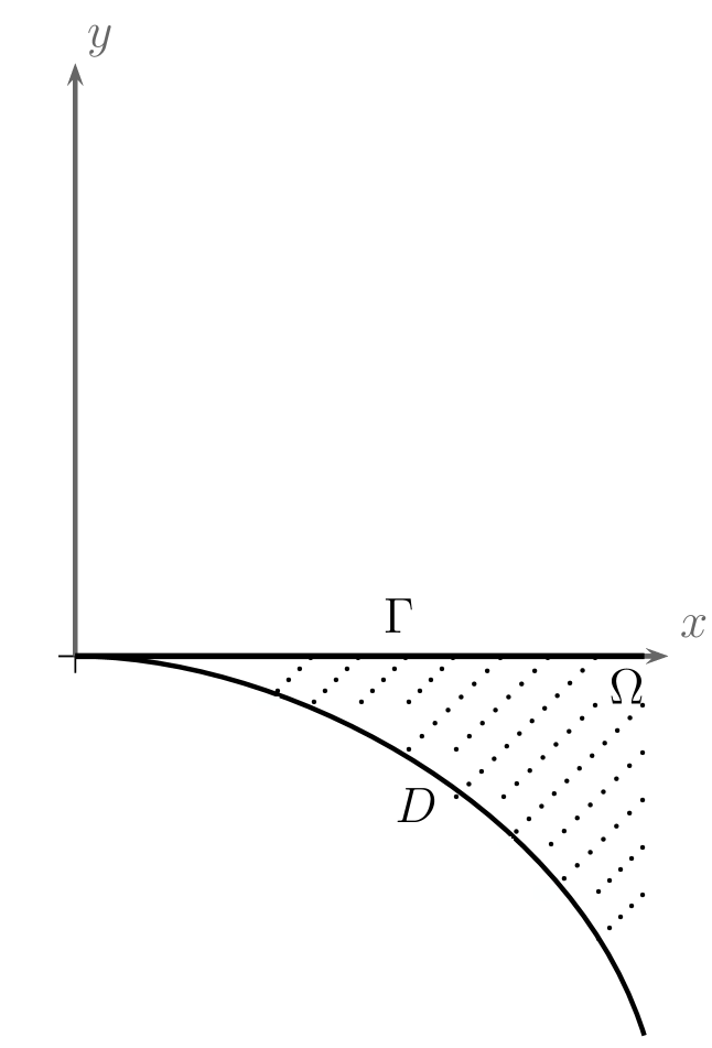
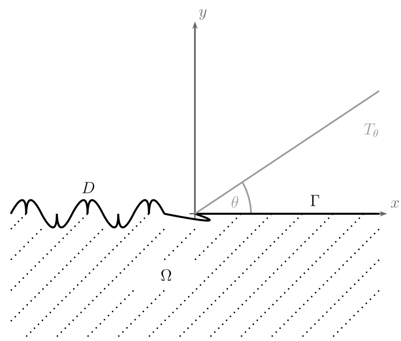
Figure 3. Situations in Example 9.6.

10. Homogeneous estimates

We provide further estimates for the extension operator from Theorem 1.2 which concern homogeneous estimates and locality (see Definition 10.1 for a proper definition). These results build on the observations made in Remark 6.11.

Definition 10.1.

An extension operator $E$ on $\mathrm{W}^{k,p}_{D}(\Omega)$ is called local if there exist constants $r_{0},\kappa>0$ such that

$$\|\nabla^{\ell}Ef\|_{\mathrm{L}^{p}(\mathrm{B}(x,r))}\lesssim\|f\|_{\mathrm{W}^{k,p}(\Omega\cap\mathrm{B}(x,\kappa r))}$$

for all $x\in\partial\Omega$, $r\in(0,r_{0})$, and $\ell\leq k$. Moreover, call $E$ homogeneous if one can replace the right-hand side of that estimate by $\|\nabla^{\ell}f\|_{\mathrm{L}^{p}(\Omega\cap\mathrm{B}(x,\kappa r))}$.

To verify that $E$ is local, we chose $F=\mathrm{B}(x,r)$ in Remark 6.11 and let $Q_{j}\in\mathcal{W}_{e}$ with $Q_{j}\cap\mathrm{B}(x,r)\neq\emptyset$. On using (5.3), (5.4), the bound on the chain length from Lemmas 5.7 as well as the properties of Whitney cubes, we see that $F(Q_{j})$ is contained in the ball $\mathrm{B}(x,\kappa r)$ for some $\kappa$ depending only on $\varepsilon$, $d$, $K$, and $\lambda$ (as before, an analogous version for $F_{P}(Q)$ holds on using Lemma 5.8 instead of Lemma 5.7 and a similar reasoning). So, with $G=\mathrm{B}(x,\kappa r)$ we derive locality from Remark 6.11 with $r_{0}=\infty$. If we restrict to $r_{0}=A\delta$, the same remark also yields that $E$ is homogeneous. Note that in the case of $\delta=\infty$ this restriction is void. We summarize this result in the following theorem.

Theorem 10.2.

Let $\Omega\subseteq\mathbb{R}^{d}$ be open and $D\subseteq\partial\Omega$ be closed such that $\Omega$ and $D$ are subject to Assumption 2.1, and fix some integer $k\geq 0$. Then there exist $A,\kappa>0$ and an extension operator $E$ such that for all $1\leq p<\infty$ one has that $E$ restricts to a bounded mapping from $\mathrm{W}^{k,p}_{D}(\Omega)$ to $\mathrm{W}^{k,p}_{D}(\mathbb{R}^{d})$ and which is moreover homogeneous and local, that is, the estimate

$$\|\nabla^{\ell}Ef\|_{\mathrm{L}^{p}(\mathrm{B}(x,r))}\lesssim\|\nabla^{\ell}f\|_{\mathrm{L}^{p}(\mathrm{B}(x,\kappa r)\cap\Omega)}$$

holds for $f\in\mathrm{W}^{k,p}_{D}(\Omega)$, $\ell\leq k$, $x\in\partial\Omega$, and $r\in(0,A\delta)$. The implicit constant in that estimate depends on $d$, $p$, $K$, $k$, $\varepsilon$, $\delta$, and $\lambda$.

References

- [1] D. R. Adams and L. I. Hedberg. Function Spaces and Potential Theory. Grundlehren der Mathematischen Wissenschaften, vol. 314, Springer, Berlin, 1996.
- [2] P. Auscher, N. Badr, R. Haller-Dintelmann, and J. Rehberg. The square root problem for second-order, divergence form operators with mixed boundary conditions on . J. Evol. Equ. 15 (2015), no. 1, 165–208.
- [3] S. Bechtel and M. Egert. Interpolation theory for Sobolev functions with partially vanishing trace on irregular open sets. J. Fourier Anal. Appl. 25 (2019), no. 5, 2733–2781.
- [4] K. Brewster, D. Mitrea, I. Mitrea, and M. Mitrea. Extending Sobolev functions with partially vanishing traces from locally -domains and applications to mixed boundary problems. J. Funct. Anal. 266 (2014), no. 7, 4314–4421.
- [5] A.-P. Calderón. Lebesgue spaces of differentiable functions and distributions. in: Proc. Sympos. Pure Math. (1961), vol. IV, 33–49.
- [6] S.-K. Chua. Extension theorems on weighted Sobolev spaces. Indiana Univ. Math. J. 41 (1992), no. 4, 1027–1076.
- [7] M. Egert. On Kato’s conjecture and mixed boundary conditions. Sierke Verlag, Göttingen, 2016.
- [8] M. Egert. -estimates for the square root of elliptic systems with mixed boundary conditions. J. Differential Equations 265 (2018), no. 4, 1279–1323.
- [9] M. Egert, R. Haller-Dintelmann, and J. Rehberg. Hardy’s inequality for functions vanishing on a part of the boundary. Potential Anal. 43 (2015), no. 1, 49–78.
- [10] M. Egert, R. Haller-Dintelmann, and P. Tolksdorf. The Kato square root problem for mixed boundary conditions. J. Funct. Anal. 267 (2014), no. 5, 1419–1461.
- [11] A. F. M. ter Elst, R. Haller-Dintelmann, J. Rehberg, and P. Tolksdorf. On the -theory for second-order elliptic operators in divergence form with complex coefficients. Available at arXiv:1903.06692.
- [12] M. Egert and P. Tolksdorf. Characterizations of Sobolev functions that vanish on a part of the boundary. Discrete Contin. Dyn. Syst. Ser. S 10 (2017), no. 4, 729–743.
- [13] A. F. M. ter Elst and J. Rehberg. Hölder estimates for second-order operators on domains with rough boundary. Adv. Differential Equations 20 (2015), no. 3-4, 299–360.
- [14] L. C. Evans and R. F. Gariepy. Measure Theory and Fine Properties of Functions. Studies in Advanced Mathematics, CRC Press, Boca Raton FL, 1992.
- [15] F. W. Gehring and B. G. Osgood. Uniform domains and the quasi-hyperbolic metric. J. Analyse Math. 36 (1979), 50–74.
- [16] F. W. Gehring and B. P. Palka. Quasiconformally homogeneous domains. J. Analyse Math. 30, 172–199.
- [17] D. Gilbarg and N. S. Trudinger. Elliptic partial differential equations of second order. Springer, Berlin, 2001.
- [18] R. Haller-Dintelmann, A. Jonsson, D. Knees, and J. Rehberg. Elliptic and parabolic regularity for second order divergence operators with mixed boundary conditions. Math. Methods Appl. Sci. 39 (2016), no. 17, 5007–5026.
- [19] D. A. Herron and P. Koskela. Conformal capacity and the quasihyperbolic metric. Indiana Univ. Math. J. 45 (1996), no. 2, 333–359.
- [20] P. W. Jones. Quasiconformal mappings and extendability of functions in Sobolev spaces. Acta Math. 147 (1981), no. 1-2, 71–88.
- [21] L. G. Rogers. Degree-independent Sobolev extension on locally uniform domains. J. Funct. Anal. 235 (2006), no. 2, 619–665.
- [22] E. M. Stein. Singular integrals and differentiability properties of functions. Princeton University Press, Princeton, 1970.
- [23] J. Taylor, S. Kim, and R. M. Brown. Heat kernel for the elliptic system of linear elasticity with boundary conditions. J. Differential Equations 257 (2014), no. 7, 2485–2519.
- [24] P. Tolksdorf. -sectoriality of higher-order elliptic systems on general bounded domains. J. Evol. Equ. 18 (2018), no. 2, 323–349.