Quantitative stability of optimal transport maps
and linearization of the $2$-Wasserstein space

Abstract.

This work studies an explicit embedding of the set of probability measures into a Hilbert space, defined using optimal transport maps from a reference probability density. This embedding linearizes to some extent the $2$-Wasserstein space, and enables the direct use of generic supervised and unsupervised learning algorithms on measure data. Our main result is that the embedding is (bi-)Hölder continuous, when the reference density is uniform over a convex set, and can be equivalently phrased as a dimension-independent Hölder-stability results for optimal transport maps.

1. Introduction

Numerous problems involve the comparison of point clouds, i.e. sets of points that lie in a metric space and for which the spatial distribution is of interest. Seeing the point clouds as discrete probability measures in a metric space, it is natural to compare them using Wasserstein distances defined by the optimal transport theory [37]. These distances have indeed been successfully used in a variety of applications in machine learning [11, 3, 25, 23, 19, 1] and in statistics [39, 12, 8, 35]. In the discrete setting, many efficient algorithms have been proposed to compute or approximate the Wasserstein distances, such as Sinkhorn-Knopp and auction algorithms – see [34] and references therein. However efficient these algorithms are, they still represent a high computational costs when dealing with large databases of point clouds . For instance, when there are $k$ point clouds, $\frac{1}{2}k(k-1)$ optimal transport problems must be solved to get the distance matrix of the database. In addition, such methods provide good approximations of Wasserstein distances but they do not allow for the direct use of machine learning algorithms based on the Wasserstein geometry. In this work, we leverage the semi-discrete formulation of optimal transport to build an explicit embedding of finitely supported probability measures over $\mathbb{R}^{d}$ into a Hilbert space. This linear embedding allows one to directly apply supervised and unsupervised learning methods on point clouds datasets consistently with the Wasserstein geometry, thus alleviating the non-Hilbertian nature of Wasserstein spaces in dimensions greater than $2$ (see for instance Section 8.3 in [34]).

1.1. Optimal transport and Monge maps

Let $\mathcal{X},$ $\mathcal{Y}$ be two compact and convex subsets of $\mathbb{R}^{d}$. Let $\rho$ be a probability density on $\mathcal{X}$ and $\mu$ be a probability measure on $\mathcal{Y}$. We consider the squared Euclidean cost $c(x,y):=\|x-y\|^{2}$ for all $x,y\in\mathbb{R}^{d}$. Monge’s formulation of the optimal transport problem consists in minimizing the transport cost over all transport maps between $\rho$ and $\mu$, that is

$$\min_{T}\left\{\int_{\mathcal{X}}c(x,T(x))\rho(x)\mathrm{d}(x)\mid T:\mathcal{X}\rightarrow\mathcal{Y},T_{\#}\rho=\mu\right\}$$, (1)

where $T_{\#}\rho$ is the pushforward measure, defined by

$$\forall B\subseteq\mathcal{Y},~{}~{}T_{\#}\rho(B)=\rho(T^{-1}(B)).$$ (2)

By the work of Brenier [9], this problem admits a solution that is uniquely defined as the gradient $T=\nabla\phi$ of a convex function $\phi$ on $\mathcal{X}$ referred to in what follows as a Brenier potential. Here, we will refer to the map $T$ as the Monge map. In this work, the source probability density $\rho\in\mathcal{P}(\mathcal{X})$ is fixed once and for all.

Definition 1.1 (Monge embedding).

Given any probability measure $\mu$ on $\mathcal{Y}$, we denote $T_{\mu}$ the solution of the optimal transport problem (1) between $\rho$ and $\mu$. We call Monge embedding the mapping

$$\mathcal{P}(\mathcal{Y}) \to L^{2}(\rho,\mathbb{R}^{d})$$ (3)

$$\mu \mapsto T_{\mu},$$

where $\mathcal{P}(\mathcal{Y})$ is the set of probability measures over $\mathcal{Y}$.

An attractive feature of the Monge embedding is that the map $T_{\mu}$ can be efficiently computed when $\mu$ is finitely supported on $\mathbb{R}^{2}$ or $\mathbb{R}^{3}$ [27], see also references in Remark 1.2. In higher dimension, they can also be estimated using stochastic optimization methods [22].

1.2. Contributions

Our main interest in this work is the regularity properties of the Monge embedding (3), or equivalently the stability of the optimal transport map in terms of the target measure. Our main theorem shows that the Monge map is a bi-Hölder embedding of $\mathcal{P}(\mathcal{Y})$ endowed with the Wasserstein distance $\mathrm{W}_{p}$ (defined in equation (10)) into the Hilbert space $L^{2}(\rho,\mathbb{R}^{d})$. More importantly, we show that the Hölder exponent does not depend on the ambient dimension $d$.

Theorem (Theorem 3.1).

Let $\rho$ be the Lebesgue measure on a compact convex subset $\mathcal{X}$ of $\mathbb{R}^{d}$ with unit volume, and let $\mathcal{Y}$ be a compact convex set. Then, for all $\mu,\nu\in\mathcal{P}(\mathcal{Y}),$ and all $p\geq 1$,

$$\mathrm{W}_{2}(\mu,\nu)\leq\|T_{\mu}-T_{\nu}\|_{\mathrm{L}^{2}(\rho)}\leq C\mathrm{W}_{p}(\mu,\nu)^{\frac{2}{15}},$$ (4)

where the constant $C$ depends on $d$, $\mathcal{X}$ and $\mathcal{Y}$.

The upper bound of this theorem should be compared to Theorem 2.3 (similar to a result of Ambrosio reported in [24]), which shows a $\frac{1}{2}$-Hölder behaviour under a very strong regularity assumption on $T_{\mu}$, and to Corollary 2.6 (from Berman, see [7]), which holds without assumption on $\mu,\nu$, but whose exponent scales exponentially badly with the dimension $d$. We conclude the article by illustrations of the behavior of this embedding, and we showcase a few applications.

Remark 1.1 (Geometric interpretation).

Similarly to [38, Eq. (3)] or [2, §10.2], one can define a distance on $\mathcal{P}(\mathcal{Y})$ using the formula

$$W_{2,\rho}(\mu,\nu):=\|T_{\mu}-T_{\nu}\|_{\mathrm{L}^{2}(\rho)},$$ (5)

and our main results reads as a bi-Hölder equivalence between this distance and the $2$-Wasserstein distance:

$$\mathrm{W}_{2}(\mu,\nu)\leq W_{2,\rho}(\mu,\nu)\leq C\mathrm{W}_{2}(\mu,\nu)^{\frac{2}{15}}.$$ (6)

Remark 1.2 (Numerical analysis interpretation).

The second inequality in (4) (and similar stability results for optimal transport maps) also has consequences in numerical analysis. Indeed, a natural way to approximate the solution of the optimal transport problem between a probability density $\rho$ and a measure $\mu$ consists in approximating $\mu$ by a sequence of measures $(\mu_{N})_{N\geq 1}$ with finite support such that $\lim_{N\to+\infty}\mathrm{W}_{1}(\mu,\mu_{N})=0$, and to approximate $T_{\mu}$ by $T_{\mu_{N}}$. This is the so-called semi-discrete approach, which can be traced back to Minkowski and Alexandrov and developed in many works from the 1990s [15, 21, 32, 10]. This approach was revisited and popularized by recent development of efficient algorithms to solve semi-discrete optimal transport problems [5, 30, 17, 29, 27, 22].

The convergence of $T_{\mu_{N}}$ to $T_{\mu}$ is well-known in optimal transport, but it usually follows from an abstract and general stability results for optimal transport maps (see Proposition 2.1), which uses compactness arguments and is therefore non-quantitative. Our main theorem gives Hölder convergence rates for the convergence of $T_{\mu_{N}}$ to $T_{\mu}$, which are in addition dimension independent.

1.3. Related work in statistics and learning

The Monge embedding (3) was introduced in [38] in the context of pattern recognition in images, were the problem of computing a distance matrix based on transportation metrics over a possibly large dataset of images is tackled. The approach proposed in [38] computes a reference image as a mean image (for the $2$-Wasserstein distance) of the whole dataset and then computes the OT maps between this reference image $\rho$ and each image $\mu_{i}$ of the training set. Distances between images are then defined based on Euclidean distances between these maps.

The geometric idea comes from a Riemannian interpretation of the Wasserstein geometry [33, 2]. In this interpretation, the tangent space to $\mathcal{P}(\mathbb{R}^{d})$ at $\rho$ is included in $L^{2}(\rho,\mathbb{R}^{d})$. The optimal transport map $T_{\mu_{i}}$ between $\rho$ and $\mu_{i}$ can then be regarded as the vector in the tangent space at $\rho$ which supports the Wasserstein geodesic from $\rho$ to $\mu_{i}$. Thus Monge’s embedding sends any probability measure $\mu_{i}$ in the (curved) manifold $\mathcal{P}(\mathbb{R}^{d})$ to a vector $T_{\mu_{i}}$ belonging to the linear space $L^{2}(\rho,\mathbb{R}^{d})$, which retain some of the geometry of the space. In the Riemannian language again, the map $\mu\mapsto T_{\mu}$ would be called a logarithm, i.e. the inverse of the Riemannian exponential map. This establishes a connection between this idea and similar strategies used to extend statistical inference notions (such as PCA) to manifold-valued data, e.g. [20, 12].

The work in [14] also proposes to use OT maps in a statistical context to overcome the lack of a canonical ordering in $\mathbb{R}^{d}$ for $d>1$. Notions of vector-quantile, vector-ranks and depth are defined based on the transport maps (and there inverses) between a reference measure defined as the uniform distribution on the unit hyperball and the $d$-dimensional samples of interest. Monge maps are also studied in [26] where an estimator for such maps between population distributions is proposed when only samples from the distributions of interest are available. Minimax estimation rates for (very) smooth transport maps in general dimension are given and the proposed estimator is shown to achieve near minimax optimality.

2. Known properties of the Monge embedding

2.1. Assumptions and notations

From now on, we fix two compact convex subsets $\mathcal{X},\mathcal{Y}$ of $\mathbb{R}^{d}$, and we fix once and for all a probability density $\rho$ on $\mathcal{X}$. For simplicity, we assume that the support of $\rho$ equals $\mathcal{X}$. We also denote $M_{\mathcal{X}}\geq 0$ the smallest positive real such that $\mathcal{X}\subset B(0,M_{\mathcal{X}})$, and $\operatorname{diam}(\mathcal{X})$ the diameter of the set $\mathcal{X}$, and similarly for $\mathcal{Y}$.

We will use the notion of potentials associated to the optimal transport problem throughout the article.

Definition 2.1 (Potentials).

Given a measure $\mu$, we denote $T_{\mu}$ the Monge map, we denote $\phi_{\mu}$ the convex Brenier potential so that $T_{\mu}=\nabla\phi_{\mu}$. We define the dual potential $\psi_{\mu}$ on $\mathcal{Y}$ as the Legendre transform of $\phi_{\mu}$:

$$\psi_{\nu}(y)=\max_{x\in\mathcal{X}}\langle x|y\rangle-\phi_{\nu}(x).$$ (7)

Adding a constant to $\phi_{\nu}$ if necessary, we assume that $\int\psi_{\nu}\mathrm{d}\nu=0$.

Remark 2.1 (Uniqueness and estimates).

The two potentials $(\phi_{\nu},\psi_{\nu})$ are closely related the Kantorovich potentials associated to the optimal transport problem (1). In our setting, where the support of $\rho$ is the whole domain $\mathcal{X}$, these potentials are unique up to addition of a constant [36, Proposition 7.18], and the constant is fixed using the condition $\int\psi_{\nu}\mathrm{d}\nu=0$.

By Eq.(7), we have the following Lipschitz estimate on $\psi_{\mu}$,

$$\mathrm{Lip}(\psi_{\mu})\leq M_{\mathcal{X}},$$ (8)

where $\mathrm{Lip}(f)$ denotes the Lipschitz constant of $f$. The assumption $\int\psi_{\mu}\mathrm{d}\mu=0$ implies that $\psi_{\mu}$ takes non-negative and non-positive values, implying that

$$\left\|\psi_{\mu}\right\|_{\infty}\leq\mathrm{Lip}(\psi_{\mu})\operatorname{diam}(\mathcal{Y})=M_{\mathcal{X}}\operatorname{diam}(\mathcal{Y}).$$ (9)

2.2. Elementary properties

A first obvious property of the embedding $\mu\mapsto T_{\mu}$ is its injectivity: if $\mu$ and $\nu$ are measures on $\mathcal{Y}$ such that $T_{\mu}=T_{\nu}$, then $(T_{\mu})_{\#}\rho=\mu=(T_{\nu})_{\#}\rho=\nu$. This injectivity ensures that the Monge embedding preserves the discriminative information about the measures it embeds. A stronger formulation of this injectivity property can be made using Wasserstein distance.

Definition 2.2 (Wasserstein distance).

The Wasserstein distance of exponent $p$ between $\mu,\nu\in\mathcal{P}(\mathcal{Y})$ is defined by

$$\mathrm{W}_{p}^{p}(\mu,\nu)=\inf_{\gamma\in\Pi(\mu,\nu)}\int_{\mathcal{Y}\times\mathcal{Y}}\|y-y^{\prime}\|^{p}d\gamma(y,y^{\prime})$$ (10)

where $\Pi(\mu,\nu)=\{\gamma\in\mathcal{M}(\mathcal{Y}\times\mathcal{Y})\mid\forall A\subset\mathcal{Y},\gamma(A\times\mathcal{Y})=\mu(A),\gamma(\mathcal{Y}\times A)=\nu(A)\}$.

Remark 2.2.

Jensen’s inequality gives $\mathrm{W}_{1}\leq\mathrm{W}_{p}$, showing that $\mathrm{W}_{1}$ is the weakest Wasserstein distance. On the other hand, since $\mathcal{Y}$ is bounded, $\mathrm{W}_{p}$ can also be bounded in terms of $\mathrm{W}_{1}$ (see [36, Eq. (5.1)]):

$$\forall\mu,\nu\in\mathcal{P}(\mathcal{Y}),~{}~{}\mathrm{W}_{1}(\mu,\nu)\leq\mathrm{W}_{p}(\mu,\nu)\leq\operatorname{diam}(\mathcal{Y})^{\frac{p-1}{p}}\mathrm{W}_{1}(\mu,\nu)^{\frac{1}{p}},$$ (11)

showing that all Wasserstein distances are in fact bi-Hölder equivalent.

Proposition 2.1.

The following properties hold:

1. The Monge embedding is reverse-Lipschitz:

   $$\forall\mu,\nu\in\mathcal{P}(Y),~{}~{}\mathrm{W}_{2}(\mu,\nu)\leq\|T_{\mu}-T_{\nu}\|_{\mathrm{L}^{2}(\rho)}.$$ (12)

2. The Monge embedding is continuous.

3. The Monge embedding is in general not better than $\frac{1}{2}$-Hölder wrt $\mathrm{W}_{2}$.

We note again that the proof of the general continuity result (ii) uses compactness arguments and is not quantitative. Our goal in the next two sections is to study the Hölder-continuity of the Monge map embedding with respect to the $1$-Wasserstein distance (which is the weakest Wasserstein distance) and to the total variation distance between measures.

Proof of Proposition 2.1.

If we denote $\gamma:=(T_{\mu},T_{\nu})_{\#}\rho$, then $\gamma\in\Pi(\mu,\nu)$. The change of variable formula gives

$$\mathrm{W}_{2}^{2}(\mu,\nu) \leq\int_{\mathcal{Y}\times\mathcal{Y}}\|y-y^{\prime}\|_{2}^{2}d\gamma(y,y^{\prime})$$

$$=\int_{\mathcal{X}}\|T_{\mu}(x)-T_{\nu}(x)\|_{2}^{2}\rho(x)\mathrm{d}x=\|T_{\mu}-T_{\nu}\|^{2}_{\mathrm{L}^{2}(\rho)},$$

showing (i). The continuity (ii) of the map $\mu\mapsto T_{\mu}$ follows from e.g. Exercise 2.17 in [37]. To prove (iii), we use the following lemma. ∎

Lemma 2.2.

Let $\rho$ be uniform on the unit disc $\mathcal{X}\subseteq\mathbb{R}^{2}$. Then, there is a curve $\theta\in[0,2\pi]\to\mu_{\theta}\in\mathcal{P}(\mathcal{X})$ and $C>0$ such that $\left\|T_{\mu_{\theta}}-T_{\mu_{0}}\right\|_{\mathrm{L}^{2}(\rho)}\geq C\mathrm{W}_{2}(\mu_{\theta},\mu_{0})^{1/2}$.

Proof.

Given $\theta\in\mathbb{R}$, we denote $x_{\theta}=(\cos\theta,\sin(\theta))$ and $\mu_{\theta}=\frac{1}{2}(\delta_{x_{\theta}}+\delta_{-x_{\theta}})$. Then, the optimal transport map between $\rho$ and $\mu_{\theta}$ is given by

$$T_{\mu_{\theta}}(x)=\begin{cases}x_{\theta}&\hbox{ if }\langle x|x_{\theta}\rangle\geq 0\\ -x_{\theta}&\hbox{ if not.}\end{cases}$$ (13)

One can easily check that for $\theta$ one has $\mathrm{W}_{2}(\mu_{0},\mu_{\theta})\leq\left|\theta\right|$. For $\theta>0$ we set

$$D_{\theta}=\{x\in\mathbb{R}^{2}\mid\langle x|x_{0}\rangle\geq 0\hbox{ and }\langle x|x_{\theta}\rangle\leq 0\}.$$ (14)

Then, on $D_{\theta}$, $T_{\mu_{\theta}}\equiv x_{-\theta}$ and $T_{\mu_{0}}\equiv x_{0}$, giving

$$\left\|T_{\mu_{\theta}}-T_{\mu_{0}}\right\|^{2}_{\mathrm{L}^{2}(\rho)}\geq\int_{D_{\theta}}\left\|x_{-\theta}-x_{0}\right\|^{2}\mathrm{d}x=\left|D_{\theta}\right|\left\|x_{-\theta}-x_{0}\right\|^{2}.$$ (15)

Moreover, if $\left|\theta\right|\leq\frac{\pi}{2}$ one has $\left\|x_{-\theta}-x_{0}\right\|^{2}\geq 2$. This gives

$$\left\|T_{\mu_{\theta}}-T_{\mu_{0}}\right\|^{2}_{\mathrm{L}^{2}(\rho)}\geq 2\left|D_{\theta}\right|\geq\frac{\left|\theta\right|}{\pi}.\qed$$

2.3. Hölder-continuity near a regular measure

We state a first result, which is a slight variant of a known stability result due to Ambrosio and reported in [24]. While [24] shows a local $1/2$-Hölder behaviour for regular enough source and target measures along a curve in the $2$-Wasserstein space, we show the same Hölder behaviour near a probability measure $\mu$ whose Monge map $T_{\mu}$ is Lipschitz continuous, but with respect to the $1$-Wasserstein distance.

Theorem 2.3.

Let $\mu,\nu\in\mathcal{P}(\mathcal{Y})$ and assume that $T_{\mu}$ is $K$-Lipschitz. Then,

$$\|T_{\mu}-T_{\nu}\|_{\mathrm{L}^{2}(\rho)}\leq 2\sqrt{M_{\mathcal{X}}K}\mathrm{W}_{1}(\mu,\nu)^{1/2}.$$ (16)

We deduce this theorem from the following elementary lemma.

Lemma 2.4.

Under the assumptions of Theorem 2.3,

$$\|T_{\mu}-T_{\nu}\|_{\mathrm{L}^{2}(\rho)}^{2}\leq 2K\int_{\mathcal{Y}}(\psi_{\nu}-\psi_{\mu})\mathrm{d}(\mu-\nu)$$ (17)

Proof.

From convex analysis, we know that the map $T_{\mu}=\nabla\phi_{\mu}$ is K-Lipschitz if and only if $\psi_{\mu}$ defined in (7) is $\frac{1}{K}$-strongly convex. We denote $A=\int_{\mathcal{Y}}\psi_{\nu}\mathrm{d}(\mu-\nu)$ and $B=\int_{\mathcal{Y}}\psi_{\mu}\mathrm{d}(\nu-\mu)$. Using that $(\nabla\phi_{\mu})_{\#}\rho=\mu$ and $(\nabla\phi_{\nu})_{\#}\rho=\nu$, we get

$$A =\int_{\mathcal{X}}(\psi_{\nu}(\nabla\phi_{\mu})-\psi_{\nu}(\nabla\phi_{\nu}))\mathrm{d}\rho$$

$$=\int_{\mathcal{X}}(\psi_{\nu}(\nabla\psi_{\mu}^{*})-\psi_{\nu}(\nabla\psi_{\nu}^{*}))\mathrm{d}\rho$$ (18)

We now use the inequality $\psi_{\nu}(y)-\psi_{\nu}(z)\geq\langle y-z|v\rangle$, which holds for all $v$ in the subdifferential $\partial\psi_{\nu}(z)$. The convex functions $\psi_{\nu},\psi_{\mu}$ are differentiable $\rho$-almost everywhere. Taking $z=\nabla\psi_{\nu}^{*}(x)$ and $y=\nabla\psi_{\mu}^{*}(x)$, and using $x\in\partial\psi_{\nu}(z)$, we obtain

$$A\geq\int_{\mathcal{X}}\langle\mathrm{id},\nabla\psi_{\mu}^{*}-\nabla\psi_{\nu}^{*}\rangle\mathrm{d}\rho$$ (19)

Using the strong convexity of $\psi_{\mu}$, we get a similar lower bound on $B$, with an extra quadratic term

$$B= \int_{\mathcal{X}}(\psi_{\mu}(\nabla\psi_{\nu}^{*})-\psi_{\mu}(\nabla\psi_{\mu}^{*}))\mathrm{d}\rho$$

$$\geq\int_{\mathcal{X}}\big{(}\langle\mathrm{id},\nabla\psi_{\nu}^{*}-\nabla\psi_{\mu}^{*}\rangle+\frac{1}{2K}\|\nabla\psi_{\nu}^{*}-\nabla\psi_{\mu}^{*}\|_{2}^{2}\big{)}\mathrm{d}\rho.$$ (20)

Summing up the lower bounds on $A$ and $B$, we get:

$$\int_{\mathcal{Y}}(\psi_{\nu}-\psi_{\mu})d(\mu-\nu)\geq \frac{1}{2K}\int_{\mathcal{X}}\|\nabla\psi_{\nu}^{*}-\nabla\psi_{\mu}^{*}\|_{2}^{2}\mathrm{d}\rho$$

$$=\frac{1}{2K}\|T_{\nu}-T_{\mu}\|_{\mathrm{L}^{2}(\rho)}^{2}.\quad\qed$$

Proof of Theorem 2.3.

Combining the Lipschitz estimate (8) this with Lemma 2.4,

$$\|T_{\mu}-T_{\nu}\|_{\mathrm{L}^{2}(\rho)}^{2} \leq 2K\int_{\mathcal{Y}}(\psi_{\nu}-\psi_{\mu})\mathrm{d}(\mu-\nu)$$

$$\leq 2K\max_{\mathrm{Lip}(f)\leq M_{\mathcal{X}}}\int_{\mathcal{Y}}f\mathrm{d}(\mu-\nu)$$

$$=2KM_{\mathcal{X}}\max_{\mathrm{Lip}(f)\leq 1}\int_{\mathcal{Y}}f\mathrm{d}(\mu-\nu)$$

$$=2KM_{\mathcal{X}}\mathrm{W}_{1}(\mu,\nu),$$ (21)

where we used Kantorovich-Rubinstein’s theorem to get the last equality. ∎

2.4. Dimension-dependent Hölder continuity

Here we assume that $\rho\equiv 1$ on a compact convex set $\mathcal{X}$ with unit volume. With no assumption on the embedded measures $\mu$ and $\nu$, another Hölder-continuity result for Monge’s embedding, can be derived from the following theorem of Berman [7].

Theorem 2.5 ([7] Proposition 3.4).

For any measures $\mu$ and $\nu$ in $\mathcal{P}(\mathcal{Y})$,

$$\|\nabla\psi_{\mu}-\nabla\psi_{\nu}\|^{2}_{\mathrm{L}^{2}(\mathcal{Y})}\leq C\Big{(}\int_{\mathcal{Y}}(\psi_{\nu}-\psi_{\mu})\mathrm{d}(\mu-\nu)\Big{)}^{\frac{1}{2^{d-1}}},$$ (22)

where $C$ depends only on $\rho$, $\mathcal{X}$ and $\mathcal{Y}$.

We deduce a global Hölder-continuity result for the Monge embedding (3). Note however that the Hölder exponent depends on the ambient dimension $d$, and the dependence is exponential. The proof of this corollary is in the appendix.

Corollary 2.6.

For any measures $\mu$ and $\nu$ in $\mathcal{P}(\mathcal{Y})$,

$$\|T_{\mu}-T_{\nu}\|_{\mathrm{L}^{2}(\rho)}\leq C\mathrm{W}_{1}(\mu,\nu)^{\frac{1}{2^{(d-1)}(d+2)}}$$ (23)

where $C$ depends only on $\rho$, $\mathcal{X}$ and $\mathcal{Y}$

3. Dimension-independent Hölder-continuity of the Monge embedding

This section is devoted to a global stability result for the Monge map embedding. As in §2.4, we require that the source measure is the Lebesgue measure $\rho\equiv 1$ on some compact convex domain $\mathcal{X}$ with unit volume, and that $\mathcal{Y}$ is bounded. Unlike Theorem 2.3, this stability result does not make any regularity assumption on the measures $\mu,\nu$. In addition, the Hölder exponent does not depend on the ambient dimension, unlike Corollary 2.6 of the previous section. We also report a stability of $\mu\mapsto T_{\mu}$ with respect to the total variation (TV) distance. This distance is much stronger than the Wasserstein distance, but the Hölder-exponent we obtain is slightly better.

Theorem 3.1 (Stability of Monge maps).

The following inequalities hold for all probability measures $\mu,\nu$ on a bounded set $\mathcal{Y}$

$$\left\|T_{\nu}-T_{\mu}\right\|_{\mathrm{L}^{2}(\mathcal{X})} \leq C\left\|\nu-\mu\right\|_{\mathrm{TV}}^{1/5}.$$ (24)

$$\left\|T_{\nu}-T_{\mu}\right\|_{\mathrm{L}^{2}(\mathcal{X})} \leq C\mathrm{W}_{1}(\mu,\nu)^{2/15},$$ (25)

where $C$ only depend on $d,\mathcal{X}$ and $\mathcal{Y}$.

The proof of this stability theorem is deduced from the stability of dual potentials, which may be interesting in its own.

Theorem 3.2 (Stability of dual potentials).

Let $\mu^{0},\mu^{1}\in\mathcal{P}(Y)$ and let $\psi^{0},\psi^{1}$ be the associated dual potentials (see Def. 2.1). Then,

$$\left\|\psi^{1}-\psi^{0}\right\|_{\mathrm{L}^{2}(\mu^{0}+\mu^{1})}\leq C\left\|\mu^{1}-\mu^{0}\right\|^{\frac{1}{2}}_{\mathrm{TV}},$$ (26)

$$\left\|\psi^{1}-\psi^{0}\right\|_{\mathrm{L}^{2}(\mu^{0}+\mu^{1})}\leq C\mathrm{W}_{1}(\mu^{1},\mu^{0})^{\frac{1}{3}},$$ (27)

where $C$ only depends on $d,\mathcal{X}$ and $\mathcal{Y}$

Remark 3.1 (Non-optimality).

The Hölder-exponent $\frac{2}{15}$ in Theorem 3.1 comes from the proof, but we see no reason why it should be the optimal exponent. Combining Theorem 3.1 with Proposition 2.1.(iii), we see that the best exponent belongs to the range $[\frac{2}{15},\frac{1}{2}]$.

Remark 3.2 (Brenier embedding).

Instead of working with the optimal transport maps $T_{\mu}$, one could also directly work with the Brenier potentials $\phi_{\mu}\in\mathrm{L}^{2}(\mathcal{X})$. A straightforward modification of the proof of Theorem 3.1 shows Hölder-continuity of the map $\mu\in\mathcal{P}(\mathcal{Y})\mapsto\phi_{\mu}\in L^{2}(\mathcal{X})$, with slightly improved exponents: the exponent would be $1/3$ with respect to the Wasserstein distance and $2/9$ with respect to the TV distance.

Remark 3.3 (McDiarmid’s inequality).

Assume that $\mu_{N},\nu_{N}$ are uniform on point clouds with $N$ points, and that their support has $N-1$ common points, i.e.

$$\mu_{N}=\frac{1}{N}\sum_{1\leq i\leq N}\delta_{y_{i}},\qquad\nu_{N}=\frac{1}{N}\sum_{2\leq i\leq N+1}\delta_{y_{i}}.$$ (28)

Then, the theorem gives $\left\|T_{\mu_{N}}-T_{\nu_{N}}\right\|\leq CN^{-1/5}$. This shows that if one considers the function

$$f(y_{1},\ldots,y_{N})=\|T_{\mu}-T_{\frac{1}{N}\sum_{i}\delta_{y_{i}}}\|_{\mathrm{L}^{2}(\rho)},$$ (29)

then,

$$| f(y_{1},\ldots,y_{i-1},y_{i},y_{i+1},\ldots,y_{N})-$$ (30)

$$f(y_{1},\ldots,y_{i-1},\hat{y}_{i},y_{i+1},\ldots,y_{N})|\leq\frac{C}{N^{-1/5}}.$$

This bound is in $N^{-1/5}$, which ensures some statistical consistency but is not enough to get concentration results with a direct use of McDiarmid’s inequality – one would need a bound in $N^{-\alpha}$ with $\alpha>\frac{1}{2}$ to use this inequality and deduce concentration results from it.

3.1. From the semi-discrete to the general case

We will establish Theorem 3.2 in the case where both measures $\mu^{0}$ and $\mu^{1}$ are supported on the same set, which is finite. We show in this section that the general case can be deduced. This follows from a simple density argument, which is summarized in the following lemma.

Lemma 3.3.

Given any $\mu^{0},\mu^{1}\in\mathcal{P}(\mathcal{Y})$, there exists sequences $(\mu^{k}_{N})_{N\geq 1}$ such that

• $\mu^{0}_{N}$ and $\mu^{1}_{N}$ have the same support, which is finite,

• $\lim\sup_{N\to+\infty}\|\mu_{N}^{0}-\mu_{N}^{1}\|_{\mathrm{TV}}\leq\|\mu^{0}-\mu^{1}\|_{\mathrm{TV}}$,

• $\lim_{N\to+\infty}\mathrm{W}_{1}(\mu^{0}_{N},\mu^{1}_{N})=\mathrm{W}_{1}(\mu^{0},\mu^{1})$,

• Denote $\psi^{k}=\psi_{\mu^{k}}$ and $\psi^{k}_{N}=\psi_{\mu^{k}_{N}}$. Then,

  $$\lim_{N\to+\infty}\left\|\psi^{1}_{N}-\psi^{0}_{N}\right\|_{\mathrm{L}^{2}(\mu^{0}_{N}+\mu^{1}_{N})}=\left\|\psi^{1}-\psi^{0}\right\|_{\mathrm{L}^{2}(\mu^{0}+\mu^{1})}.$$ (31)

Proof.

For any $N>0$, we consider a finite partition $\mathcal{Y}=\sqcup_{1\leq i\leq N}\mathcal{Y}^{N}_{i}$, we let $\varepsilon_{N}=\max_{i}\operatorname{diam}(\mathcal{Y}_{i}^{N})$ and we assume that $\lim_{N\to+\infty}\varepsilon_{N}=0$. Then, we define

$$\mu^{k}_{N}=\sum_{1\leq i\leq N}\left[\left(1-\frac{1}{N}\right)\mu^{k}(\mathcal{Y}_{i}^{N})+\frac{1}{N^{2}}\right]\delta_{y_{i}^{N}},$$ (32)

where $y_{i}^{N}\in\mathcal{Y}_{i}^{N}$. Then, it is easy to check that the support of the measures $\mu^{0}_{N}$ and $\mu^{1}_{N}$ is the set $\{y_{1}^{N},\ldots,y^{N}_{N}\}$. Moreover,

$$\left\|\mu^{1}_{N}-\mu^{0}_{N}\right\|_{\mathrm{TV}}\leq\left\|\mu^{1}-\mu^{0}\right\|_{\mathrm{TV}}.$$ (33)

In addition, $\mathrm{W}_{1}(\mu^{k}_{N},\mu^{k})\leq\varepsilon_{N}\xrightarrow{N\to+\infty}0.$ Combined with the triangle inequality, we deduce

$$|\mathrm{W}_{1}(\mu^{0}_{N},\mu^{1}_{N})-\mathrm{W}_{1}(\mu^{0},\mu^{1})| =|\mathrm{W}_{1}(\mu^{0}_{N},\mu^{1}_{N})-\mathrm{W}_{1}(\mu^{0}_{N},\mu^{1})+\mathrm{W}_{1}(\mu^{0}_{N},\mu^{1})-\mathrm{W}_{1}(\mu^{0},\mu^{1})|$$

$$\leq|\mathrm{W}_{1}(\mu^{0}_{N},\mu^{1}_{N})-\mathrm{W}_{1}(\mu^{0}_{N},\mu^{1})|+|\mathrm{W}_{1}(\mu^{0}_{N},\mu^{1})-\mathrm{W}_{1}(\mu^{0},\mu^{1})|$$

$$\leq\mathrm{W}_{1}(\mu^{1}_{N},\mu^{1})+\mathrm{W}_{1}(\mu^{0}_{N},\mu^{0})$$

$$\leq 2\varepsilon_{N}\xrightarrow{N\to+\infty}\mathrm{W}_{1}(\mu^{0},\mu^{1})$$ (34)

The last statement also follows from standard arguments from optimal transport, which we summarize now. By (8)–(9), we know that the sequences $(\psi^{k}_{N})$ are uniformly bounded and uniformly Lipschitz. By Arzelà-Ascoli’s theorem, this implies that the sequence $(\psi^{k}_{N})$ admits a subsequence converging uniformly to some $\tilde{\psi}^{k}$. By [36, Theorem 1.51], $\tilde{\psi}^{k}$ is a Kantorovich potential for the optimal transport problem between $\rho$ and $\mu^{k}$. Since in addition,

$$0=\lim_{N\to+\infty}\int\psi^{k}_{N}\mathrm{d}\mu^{k}_{N}=\int\tilde{\psi}^{k}\mathrm{d}\mu^{k},$$ (35)

we obtain, by Remark 2.1 that $\tilde{\psi}^{k}=\psi^{k}$. This shows that the whole sequence $\psi^{k}_{N}$ converges uniformly to $\psi^{k}$. This implies as desired

$$\lim_{N\to+\infty}\int(\psi^{1}_{N}-\psi^{0}_{N})^{2}\mathrm{d}(\mu^{0}_{N}+\mu^{1}_{N})=\int(\psi^{1}-\psi^{0})^{2}\mathrm{d}(\mu^{0}+\mu^{1}).\qed$$

3.2. Semi-discrete optimal transport

In the remaining of this section, we work in the semi-discrete setting, assuming that all measures are supported on a (fixed) set $\{y_{1},\ldots,y_{N}\}$. Assuming that $\mu=\sum_{1\leq i\leq N}\mu_{i}\delta_{y_{i}}$, the Kantorovich dual to the optimal transport problem between $\rho$ and $\mu$ problem can be written as (e.g. [26, Eq. (2.6)]):

$$\mathrm{(D)}=\min_{\psi}\int_{\mathcal{X}}\psi^{*}\mathrm{d}\rho+\int_{\mathcal{Y}}\psi\mathrm{d}\mu$$ (36)

where the minimum is taken among functions $\psi$ on $\{y_{1},\ldots,y_{N}\}$. To simplify notations, we will often conflate the function $\psi$ with the vector $\bm{\psi}\in\mathbb{R}^{N}$ defined by $\bm{\psi}_{i}=\psi(y_{i})$. This vector $\bm{\psi}$ is also referred to as a (dual) potential and defines a partition of the domain $\mathcal{X}$ into so-called Laguerre cells, described for all $1\leq i\leq N$ by

$$V_{i}(\bm{\psi})=\{x\in\mathcal{X}\mid\forall j,\bm{\psi}_{j}\geq\bm{\psi}_{i}+\langle y_{j}-y_{i}|x\rangle\},$$ (37)

so that

$$\mathrm{(D)}=\min_{\bm{\psi}\in\mathbb{R}^{N}}\mathcal{K}(\bm{\psi})$$ (38)

$$\hbox{ where }\mathcal{K}(\bm{\psi})=\sum_{i=1}^{N}\int_{V_{i}(\bm{\psi})}(\langle x|y_{i}\rangle-\bm{\psi}_{i})\mathrm{d}\rho(x)+\sum_{i=1}^{N}\mu_{i}\bm{\psi}_{i}.$$ (39)

By Theorem 1.1 in [27] (see also [5]),

$$\nabla\mathcal{K}=G(\bm{\psi})-\nu$$ (40)

where

$$G_{i}(\bm{\psi})=\rho(V_{i}(\bm{\psi}))$$ (41)

$$G(\bm{\psi})=(G_{i}(\bm{\psi}))_{1\leq i\leq N}\in\mathbb{R}^{N}.$$ (42)

Therefore, a potential $\bm{\psi}$ solves problem (38) if and only if $G(\bm{\psi})=\nu$. The optimal potential $\bm{\psi}$ in (38) then defines a Monge map $T:\mathcal{X}\rightarrow\mathcal{Y}$ that is piecewise constant, sending each point $x$ in $V_{i}(\bm{\psi})$ to $y_{i}$. Alternatively, one can define $T=\nabla\phi$ where $\phi=\psi^{*}$ is the Legendre transform of the function $\psi$ defined by $\psi(y_{i})=\bm{\psi}_{i}$. Given a potential $\bm{\psi}\in\mathbb{R}^{N}$, we denote

$$\mu_{\bm{\psi}}=\sum_{1\leq i\leq N}G_{i}(\bm{\psi})\delta_{y_{i}}.$$ (43)

Jacobian of $G$

We consider the set $S_{+}\subseteq\mathbb{R}^{N}$ of potentials such that all Laguerre cells $V_{i}(\bm{\psi})$ contain some mass, defined by

$$S_{+}=\{\bm{\psi}\in\mathbb{R}^{N}\mid\forall i,G_{i}(\bm{\psi})>0\}.$$ (44)

From Theorems 1.3 and 4.1 in [27], we know that the map $G$ is $\mathcal{C}^{1}$ on the set $S_{+}$. By Theorem 1.3 in [27], if $\bm{\psi}\in S_{+}$, the partial derivatives of $G$ are given by

$$\begin{cases}\frac{\partial G_{i}}{\partial\bm{\psi}_{j}}(\bm{\psi})=\frac{\mathrm{vol}^{d-1}(V_{i}(\bm{\psi})\cap V_{j}(\bm{\psi}))}{\left\|y_{j}-y_{i}\right\|}&\hbox{ for }i\neq j\\ \frac{\partial G_{i}}{\partial\bm{\psi}_{i}}(\bm{\psi})=-\sum_{j\neq i}\frac{\partial G_{i}}{\partial\bm{\psi}_{j}}(\bm{\psi})\end{cases}$$ (45)

3.3. Proof of Theorem 3.2 (Stability of potentials) in the semi-discrete case

In this section, we prove Theorem 3.2 when the measures $\mu,\nu$ have the same finite support. This version of Theorem 3.2 is rephrased as Theorem 3.4.

Theorem 3.4.

Let $\bm{\psi}^{0},\bm{\psi}^{1}$ be two potentials in $S_{+}$ satisfying

$$\langle\bm{\psi}^{0}|G(\bm{\psi}^{0})\rangle_{\mathbb{R}^{N}}=\langle\bm{\psi}^{1}|G(\bm{\psi}^{1})\rangle_{\mathbb{R}^{N}}=0.$$ (46)

Then, with $\mu^{k}=\mu_{\bm{\psi}^{k}},$

$$\langle(\bm{\psi}^{1}-\bm{\psi}^{0})^{2}|G(\bm{\psi}^{0})+G(\bm{\psi}^{1})\rangle_{\mathbb{R}^{N}}\leq C\left\|\mu^{1}-\mu^{0}\right\|_{\mathrm{TV}}.$$ (47)

$$\langle(\bm{\psi}^{1}-\bm{\psi}^{0})^{2}|G(\bm{\psi}^{0})+G(\bm{\psi}^{1})\rangle_{\mathbb{R}^{N}}\leq C\mathrm{W}_{1}(\mu^{1},\mu^{0})^{\frac{2}{3}},$$ (48)

where $C$ depends only on $d,\mathcal{X}$ and $\mathcal{Y}$.

We will require two preliminary results. The next lemma follows from Brunn-Minkowski’s inequality. This inequality has already appeared in the numerical analysis of Monge-Ampère equations, see [6, 31].

Lemma 3.5.

Let $\bm{\psi}^{0},\bm{\psi}^{1}\in S^{+}$ and consider $\bm{\psi}^{t}=(1-t)\bm{\psi}^{0}+t\bm{\psi}^{1}$. Then,

$$\forall i,~{}G_{i}(\bm{\psi}^{t})^{\frac{1}{d}}\geq(1-t)G_{i}(\bm{\psi}^{0})^{\frac{1}{d}}+tG_{i}(\bm{\psi}^{1})^{\frac{1}{d}}$$ (49)

In particular, $\bm{\psi}^{t}\in S^{+}$. Moreover,

$$\left\|G(\bm{\psi}^{t})-G(\bm{\psi}^{0})\right\|_{1}\leq\left\|G(\bm{\psi}^{1})-G(\bm{\psi}^{0})\right\|_{1},$$ (50)

$$\left\|G(\bm{\psi}^{t})-G(\bm{\psi}^{0})\right\|_{1}\leq 2(1-(1-t)^{d}).$$ (51)

Proof.

Let $x^{0}\in V_{i}(\bm{\psi}^{0})$ and $x^{1}\in V_{i}(\bm{\psi}^{1})$. Then, for all $j\in\{1,\dots,N\}$,

$$\begin{cases}\bm{\psi}^{0}_{j}\geq\bm{\psi}^{0}_{i}+\langle y_{j}-y_{i}|x^{0}\rangle\\ \bm{\psi}^{1}_{j}\geq\bm{\psi}^{1}_{i}+\langle y_{j}-y_{i}|x^{1}\rangle.\\ \end{cases}$$ (52)

Taking the convex combination of these inequalities we get for all $j\in\{1,\dots,N\}$,

$$\bm{\psi}^{t}_{j}\geq\bm{\psi}^{t}_{i}+\langle y_{j}-y_{i}|(1-t)x^{0}+tx^{1}\rangle.$$ (53)

This shows that $(1-t)x^{0}+tx^{1}\in V_{i}(\bm{\psi}^{t})$ (note that we use the convexity of $\mathcal{X}$ here). Thus,

$$(1-t)V_{i}(\bm{\psi}^{0})+tV_{i}(\bm{\psi}^{1})\subseteq V_{i}(\bm{\psi}^{t}).$$ (54)

Taking the Lebesgue measure on both sides and applying Brunn-Minkowski’s inequality gives

$$G_{i}(\bm{\psi}^{t})^{1/d}=\rho(V_{i}(\bm{\psi}^{t}))^{1/d} \geq\rho((1-t)V_{i}(\bm{\psi}^{0})+tV_{i}(\bm{\psi}^{1}))^{1/d}$$ (55)

$$\geq(1-t)\rho(V_{i}(\bm{\psi}^{0}))^{1/d}+t\rho(V_{i}(\bm{\psi}^{1}))^{1/d}$$

$$\geq(1-t)G_{i}(\bm{\psi}^{0})^{1/d}+tG_{i}(\bm{\psi}^{1}))^{1/d}$$

This inequality directly implies

$$G_{i}(\bm{\psi}^{t})\geq\min(G_{i}(\bm{\psi}^{0}),G_{i}(\bm{\psi}^{1})),$$ (56)

$$\hbox{i.e.}\min(G_{i}(\bm{\psi}^{t}),G_{i}(\bm{\psi}^{0}))\geq\min(G_{i}(\bm{\psi}^{0}),G_{i}(\bm{\psi}^{1})).$$

Using the following equivalent formulation of the TV distance between probability measures we get (50):

$$\frac{1}{2}\left\|G(\bm{\psi}^{t})-G(\bm{\psi}^{0})\right\|_{1} =1-\sum_{i}\min(G_{i}(\bm{\psi}^{t}),G_{i}(\bm{\psi}^{0}))$$ (57)

$$\leq 1-\sum_{i}\min(G_{i}(\bm{\psi}^{0}),G_{i}(\bm{\psi}^{1}))=\frac{1}{2}\left\|G(\bm{\psi}^{t})-G(\bm{\psi}^{0})\right\|_{1}.$$

To prove (51), we first remark that by (49),

$$G_{i}(\bm{\psi}^{t})\geq(1-t)^{d}G_{i}(\bm{\psi}^{0}),$$ (58)

$$\hbox{i.e.}\min(G_{i}(\bm{\psi}^{t}),G_{i}(\bm{\psi}^{0}))\geq(1-t)^{d}G_{i}(\bm{\psi}^{0}).$$

We conclude using the same formula as above:

$$\frac{1}{2}\left\|G(\bm{\psi}^{t})-G(\bm{\psi}^{0})\right\|_{1} =1-\sum_{i}\min(G_{i}(\bm{\psi}^{t}),G_{i}(\bm{\psi}^{0}))$$ (59)

$$\leq 1-\sum_{i}(1-t)^{d}G_{i}(\bm{\psi}^{0})=1-(1-t)^{d}.$$

∎

The next proposition gives an explicit lower bound on the smallest non-zero eigenvalue of the opposite of Jacobian matrix of the map $G$. Its proof follows from the stability analysis of finite volumes discretization of elliptic PDEs, see Lemma 3.7 in [18]. We report this proof (with very minor adaptations to our case) in the appendix.

Proposition 3.6 (Discrete Poincaré-Wirtinger inequality).

Consider $\bm{\psi}\in S_{+}$ and $v\in\mathbb{R}^{N}$. Then,

$$\langle v^{2}|G(\bm{\psi})\rangle_{\mathbb{R}^{N}}-\langle v|G(\bm{\psi})\rangle^{2}_{\mathbb{R}^{N}}\leq-C\langle\mathrm{D}G(\bm{\psi})v|v\rangle_{\mathbb{R}^{N}}$$ (60)

where $C=C(d)\operatorname{diam}(\mathcal{Y})\operatorname{diam}(\mathcal{X})^{d+1}>0$.

Remark 3.4.

In particular, $-\mathrm{D}G(\bm{\psi})$ is semidefinite positive, since its smallest non-zero eigenvalue is greater than a variance. This can also be seen from the definition of $\mathrm{D}G(\bm{\psi})$ as a Laplacian matrix, or simply from Gershgorin’s circle theorem and the explicit formula for $\mathrm{D}G(\bm{\psi})$ recalled in (45).

With these two results at hand, we show $L^{2}$ stability of the dual potentials in the semi-discrete case.

Proof of Theorem 3.4.

In this proof, $A\lesssim B$ means that $A\leq CB$ for a constant $C$ depending only on $d$, the diameters of $\mathcal{X}$ and $\mathcal{Y}$, $M_{\mathcal{X}}$ and $M_{\mathcal{Y}}$. Denote $\bm{\psi}^{t}=(1-t)\bm{\psi}^{0}+t\bm{\psi}^{1}$ and $v=\bm{\psi}^{1}-\bm{\psi}^{0}$. By Taylor’s formula,

$$\langle G(\bm{\psi}^{1})-G(\bm{\psi}^{0})|v\rangle_{\mathbb{R}^{N}}=\int_{0}^{1}\langle\mathrm{D}G(\bm{\psi}^{t})v|v\rangle_{\mathbb{R}^{N}}\mathrm{d}t$$ (61)

Moreover, Proposition 3.6 gives

$$\langle v^{2}|G(\bm{\psi}^{t})\rangle_{\mathbb{R}^{N}}-\langle v|G(\bm{\psi}^{t})\rangle^{2}_{\mathbb{R}^{N}}\lesssim-\langle\mathrm{D}G(\bm{\psi}^{t})v|v\rangle_{\mathbb{R}^{N}}$$ (62)

Let us restrict to $t\in[0,\frac{1}{4}]$. Then, by Eq. (49), one has

$$G_{i}(\bm{\psi}^{t})\geq(1-t)^{d}G_{i}(\bm{\psi}^{0})\gtrsim G_{i}(\bm{\psi}^{0}),$$ (63)

Thus, on the interval $t\in[0,\frac{1}{4}]$,

$$\langle v^{2}|G(\bm{\psi}^{0})\rangle\lesssim\langle v^{2}|G(\bm{\psi}^{t})\rangle.$$ (64)

On the other hand, using the assumption (46), we get

$$\langle v|G(\bm{\psi}^{t})\rangle_{\mathbb{R}^{N}} =\langle\bm{\psi}^{1}-\bm{\psi}^{0}|G(\bm{\psi}^{t})\rangle_{\mathbb{R}^{N}}$$

$$=\langle\bm{\psi}^{1}-\bm{\psi}^{0}|G(\bm{\psi}^{t})-G(\bm{\psi}^{0})\rangle_{\mathbb{R}^{N}}+\langle\bm{\psi}^{1}-\bm{\psi}^{0}|G(\bm{\psi}^{0})\rangle_{\mathbb{R}^{N}}$$

$$=\langle\bm{\psi}^{1}-\bm{\psi}^{0}|G(\bm{\psi}^{t})-G(\bm{\psi}^{0})\rangle_{\mathbb{R}^{N}}+\langle\bm{\psi}^{1}|G(\bm{\psi}^{0})-G(\bm{\psi}^{1})\rangle_{\mathbb{R}^{N}}$$ (65)

thus implying

$$\left|\langle v|G(\bm{\psi}^{t})\rangle\right| \leq\left\|\bm{\psi}_{1}-\bm{\psi}_{0}\right\|_{\infty}\left\|G(\bm{\psi}^{t})-G(\bm{\psi}^{0})\right\|_{1}+\mathrm{Lip}(\bm{\psi}_{1})\mathrm{W}_{1}(\mu_{0},\mu_{1})$$

$$\lesssim\left\|G(\bm{\psi}^{t})-G(\bm{\psi}^{0})\right\|_{1}+\mathrm{W}_{1}(\mu_{0},\mu_{1})$$ (66)

where we used Kantorovich-Rubinstein’s theorem to get the first inequality and that $\left\|\bm{\psi}_{1}-\bm{\psi}_{0}\right\|_{\infty}$ is bounded by a constant depending on $\mathcal{X}$ and $\mathcal{Y}$, as in (9). Using Kantorovich-Rubinstein’s theorem again, we also get

$$\left|\langle G(\bm{\psi}^{1})-G(\bm{\psi}^{0})|v\rangle\right| \lesssim\mathrm{W}_{1}(\mu^{0},\mu^{1})$$ (67)

$$\lesssim\left\|\mu^{0}-\mu^{1}\right\|_{\mathrm{TV}}.$$

Proposition 3.6 implies that $\langle\mathrm{D}G(\bm{\psi}^{t})v|v\rangle\leq 0$ for all $t\in[0,1]$. Combining (61),(62),(64), (66) and (67) gives us

$$T\langle v^{2}|G(\bm{\psi}^{0})\rangle\lesssim\mathrm{W}_{1}(\mu^{0},\mu^{1})+\int_{0}^{T}(\left\|G(\bm{\psi}^{t})-G(\bm{\psi}^{0})\right\|_{1}+\mathrm{W}_{1}(\mu_{0},\mu_{1}))^{2}\mathrm{d}t$$ (68)

To conclude the proof of the stability with respect to the total variation norm (47), we simply note that thanks to Lemma 3.5 (50), we have $\left\|G(\bm{\psi}^{t})-G(\bm{\psi}^{0})\right\|_{1}\leq\left\|G(\bm{\psi}^{1})-G(\bm{\psi}^{0})\right\|_{1}$. Combining with the comparison $\mathrm{W}_{1}\lesssim\left\|\cdot\right\|_{\mathrm{TV}}$, (68) with $T=\frac{1}{4}$ yields

$$\langle v^{2}|G(\bm{\psi}^{0})\rangle\lesssim\left\|\mu^{1}-\mu^{0}\right\|_{\mathrm{TV}}.$$ (69)

Note that thanks to symmetry, we get the same upper bound with $G(\bm{\psi}^{0})$ replaced by $G(\bm{\psi}^{1})$. Summing these bounds thus concludes the proof of (47).

To get the second stability inequality (48), with respect to the Wasserstein distance, we use Lemma 3.5–(51), which gives for $t\in[0,T],$

$$\left\|G(\bm{\psi}^{t})-G(\bm{\psi}^{0})\right\|_{1}\leq 2(1-(1-t)^{d})\lesssim T.$$ (70)

Combining this inequality with Eq. (68) we get for $T\leq\frac{1}{4}$,

$$T\langle v^{2}|G(\bm{\psi}^{0})\rangle\lesssim\mathrm{W}_{1}(\mu^{0},\mu^{1})+T(T+\mathrm{W}_{1}(\mu_{0},\mu_{1}))^{2}.$$ (71)

If $\mathrm{W}_{1}(\mu^{0},\mu^{1})^{\frac{1}{3}}\leq\frac{1}{4}$, we can choose $T=\mathrm{W}_{1}(\mu^{0},\mu^{1})^{\frac{1}{3}}$ to obtain the desired inequality (48). On the other hand, if $\mathrm{W}_{1}(\mu^{0},\mu^{1})^{\frac{1}{3}}\geq\frac{1}{4}$, taking $T=\frac{1}{4}$ gives us

$$\langle v^{2}|G(\bm{\psi}^{0})\rangle\lesssim\mathrm{W}_{1}(\mu^{0},\mu^{1})=D\frac{\mathrm{W}_{1}(\mu,\nu)}{D}\leq D\left(\frac{\mathrm{W}_{1}(\mu,\nu)}{D}\right)^{2/3}$$ (72)

with $D:=\max_{\mu,\nu\in\mathcal{P}(\mathcal{Y})}\mathrm{W}_{1}(\mu,\nu)\leq\operatorname{diam}(\mathcal{Y})$ thus also proving (48) in that case. ∎

3.4. Proof of Theorem 3.1 (Stability of optimal transport maps)

We need a result from [13], providing an upper bounds the $L^{2}$ norm between gradients of convex functions.

Proposition 3.7 ([13] Theorem 22).

Let $f$ and $g$ be convex functions on a bounded convex set $\mathcal{X}$, then

$$\|\nabla f-\nabla g\|_{\mathrm{L}^{2}}\leq 2C_{\mathcal{X}}\|f-g\|_{\infty}^{1/2}(\|\nabla f\|_{\infty}^{1/2}+\|\nabla g\|_{\infty}^{1/2})$$ (73)

where $C_{\mathcal{X}}$ depends only on $\mathcal{X}$.

The stability of potentials (Theorem 3.4) implies that

$$\|\psi^{0}-\psi^{1}\|_{\mathrm{L}^{2}(\mu^{0}+\mu^{1})}^{2}\lesssim\varepsilon$$ (74)

$$\hbox{ with }\varepsilon=\|\mu^{0}-\mu^{1}\|_{\mathrm{TV}}\hbox{ or }\varepsilon=\mathrm{W}_{1}(\mu^{0},\mu^{1})^{\frac{2}{3}}.$$

In practice, these $L^{2}$ estimates are not sufficient to conclude, and we need to translate them into a $L^{\infty}$ estimate in order to apply Proposition 3.7. For this purpose, we consider $\alpha\in(0,1)$, and we define

$$\mathcal{Y}_{\alpha}=\{y\in\mathcal{Y}\mid\left|\psi^{0}(y)-\psi^{1}(y)\right|\leq\varepsilon^{\alpha}\}.$$ (75)

By Chebyshev’s inequality, we deduce from (74) that for $k\in\{0,1\},$

$$\varepsilon^{2\alpha}\mu^{k}(\mathcal{Y}\setminus\mathcal{Y}_{\alpha})\leq\left\|\psi^{0}-\psi^{1}\right\|^{2}_{\mathrm{L}^{2}(\mu^{k})}\lesssim\varepsilon,$$ (76)

which gives

$$1-\mu^{k}(\mathcal{Y}_{\alpha})\lesssim\varepsilon^{1-2\alpha}.$$ (77)

We construct the Legendre transform of the functions $\psi^{k}$ on the whole set $\mathcal{Y}$, and of the restrictions of $\psi^{k}$ to the set $\mathcal{Y}_{\alpha}$:

$$\phi^{k}(x) =\max_{y\in\mathcal{Y}}\langle x|y\rangle-\psi^{k}(y),$$ (78)

$$\phi^{k,\alpha}(x) =\max_{y\in\mathcal{Y}_{\alpha}}\langle x|y\rangle-\psi^{k}(y).$$ (79)

Comparing Eqs. (78) and (79), one sees that $\phi^{k,\alpha}\leq\phi^{k}$. Moreover, if $\nabla\phi^{k}(x)\in\mathcal{Y}_{\alpha}$, then using the Fenchel-Young (in)equality,

$$\phi^{k}(x)+\psi^{k}(\nabla\psi^{k}(x))=\langle x|\nabla\psi^{k}(x)\rangle\leq\phi^{k,\alpha}(x)+\psi^{k,\alpha}(\nabla\psi^{k}(x)),$$ (80)

so that $\phi^{k}(x)=\phi^{k,\alpha}(x)$. In other words, $\phi^{k,\alpha}\equiv\phi^{k}$ on the set

$$\mathcal{X}_{\alpha}=(\nabla\phi^{k})^{-1}(\mathcal{Y}_{\alpha}).$$ (81)

Note also that this set $\mathcal{X}_{\alpha}^{k}$ is "large", in the sense that

$$1-\rho(\mathcal{X}_{\alpha}^{k}) =1-\rho((\nabla\phi^{k})^{-1}(\mathcal{Y}_{\alpha}))$$ (82)

$$=1-\mu^{k}(\mathcal{Y}_{\alpha})\lesssim\varepsilon^{1-2\alpha},$$

where we used $\nabla\phi^{k}_{\#}\rho=\mu^{k}$. As in (8), the gradients $\nabla\phi^{k,\alpha}$ and $\nabla\phi^{k}$ are uniformly bounded by $M_{\mathcal{Y}}$ (by Eqs. (78) and (79)) and they coincide on the "large" set $\mathcal{X}_{\alpha}^{k}$. This directly implies that they are close in $L^{2}$ norm:

$$\|\nabla\phi^{k,\alpha}-\nabla\phi^{k}\|_{\mathrm{L}^{2}(\mathcal{X})} =\|\nabla\phi^{k,\alpha}-\nabla\phi^{k}\|_{\mathrm{L}^{2}(\mathcal{X}\setminus\mathcal{X}^{k}_{\alpha})}$$ (83)

$$\quad\leq(1-\rho(\mathcal{X}^{k}_{\alpha}))(\|\nabla\phi^{k,\alpha}\|_{\infty}+\|\nabla\phi^{k}\|_{\infty})\lesssim\varepsilon^{1-2\alpha}.$$

On the other hand, by definition of $\mathcal{Y}_{\alpha}$ (see Eq. (75)), the functions $\psi^{0}$ and $\psi^{1}$ are uniformly close on the set $\mathcal{Y}_{\alpha}.$ This implies that the Legendre transforms $\phi^{0,\alpha}$ and $\phi^{1,\alpha}$, defined in (79), are also close. Indeed,

$$\phi^{0,\alpha}(x) =\max_{y\in\mathcal{Y}^{\alpha}}\langle x|y\rangle-\psi^{0}(x)$$ (84)

$$\leq\max_{y\in\mathcal{Y}^{\alpha}}\langle x|y\rangle-\psi^{1}(x)+\varepsilon^{\alpha}$$

$$=\phi^{1,\alpha}(x)+\varepsilon^{\alpha},$$

thus giving by symmetry

$$\|\phi^{1,\alpha}-\phi^{0,\alpha}\|_{\infty}\leq\varepsilon^{\alpha}.$$ (85)

Combining this inequality with Proposition 3.7, we obtain

$$\|\nabla\phi^{1,\alpha}-\nabla\phi^{0,\alpha}\|_{\mathrm{L}^{2}(\mathcal{X})}\lesssim 2(\|\nabla\phi^{0,\alpha}\|_{\infty}+\|\nabla\phi^{1,\alpha}\|_{\infty})^{1/2}\|\phi^{1,\alpha}-\phi^{0,\alpha}\|_{\infty}^{1/2}\lesssim\varepsilon^{\frac{\alpha}{2}}$$ (86)

Using the triangle inequality and the two previous estimations (83)–(86), we obtain

$$\|\nabla\phi^{1}-\nabla\phi^{0}\|_{\mathrm{L}^{2}(\mathcal{X})}$$

$$\leq\|\nabla\phi^{1}-\nabla\phi^{1,\alpha}\|_{\mathrm{L}^{2}(\mathcal{X})}+\|\nabla\phi^{1,\alpha}-\nabla\phi^{0,\alpha}\|_{\mathrm{L}^{2}(\mathcal{X})}+\|\nabla\phi^{0,\alpha}-\nabla\phi^{0}\|_{\mathrm{L}^{2}(\mathcal{X})}$$

$$\lesssim\varepsilon^{1-2\alpha}+\varepsilon^{\alpha/2}$$ (87)

The best exponent is obtained when $1-2\alpha=\alpha/2$ i.e. $1=5\alpha/2$, $\alpha=2/5$, giving

$$\|\nabla\phi^{1}-\nabla\phi^{0}\|_{\mathrm{L}^{2}(\mathcal{X})}\lesssim\varepsilon^{\frac{1}{5}},$$ (88)

which implies the desired estimates if one replaces $\varepsilon$ with the possible values (74).

4. Experiments

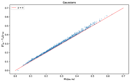
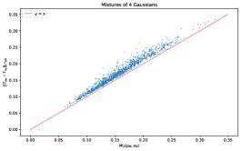
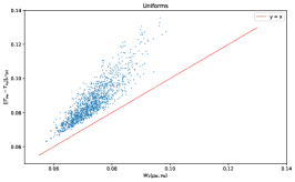
Figure 1. $W_{2,\rho}$ vs. $\mathrm{W}_{2}$ between point clouds sampled from Gaussian, Mixture of 4 Gaussian and Uniform distributions. $\mathrm{W}_{2}$ being approximated with entropic regularization, we may have $\mathrm{W}_{2}\geq W_{2,\rho}$ on certain points.

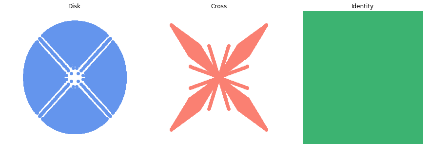
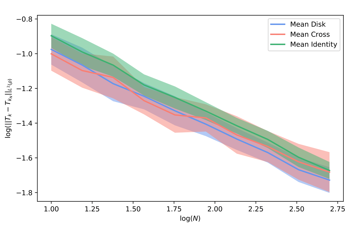
Figure 2. (Left) Target measures, push-forwards of the maps $T_{k}=\nabla\phi_{k}$ where $\phi_{\text{Disk}}(x,y):=0.25(x+y)+0.07(|x+y|^{3/2}+|x-y|^{3/2})$, $\phi_{\text{Cross}}(x,y):=0.5(x+y)+0.04\max(4(x+y-1)^{2}+0.5(2x-1)^{2}+0.5(2y-1)^{2},4(x-y)^{2}+0.5(2x-1)^{2}+0.5*(2y-1)^{2})$ and $\phi_{\text{Square}}(x,y):=0.5(x^{2}+y^{2})$ (Right) Sampling distance $\|T_{\mu}-T_{\mu_{N}}\|_{\mathrm{L}^{2}(\rho)}$.

In this last section, we briefly illustrate the behaviour of the Monge map embeddings and we mention potential use of these embeddings in machine learning. In what follows, we consider that $d=2$ and that $\rho$ is the Lebesgue measure on the unit square $\mathcal{X}=[0,1]^{2}$. For simplicity, the discrete measures $\mu$ and $\nu$ are also supported on $\mathcal{Y}=\mathcal{X}$, for which algorithms readily give approximates of $\mathrm{W}_{p}(\mu,\nu)$ and of $T_{\mu}$ or $T_{\nu}$. The Wasserstein distance $\mathrm{W}_{p}(\mu,\nu)$ is approximated using Sinkhorn’s algorithm [16] while $T_{\mu}$ and $T_{\nu}$ are approximated with a damped Newton’s algorithm [27].

4.1. Vectorization of the Monge maps

The Hilbert space $H=\mathrm{L}^{2}(\rho,\mathbb{R}^{2})$, which contains the Monge maps $T_{\mu},T_{\nu}$ is infinite dimensional. We therefore project the maps on the finite dimensional subspace $H_{m}\subseteq H$ of piecewise constant maps, defined for any $m\in\mathbb{N}$ by

$$H_{m}=\{T\in\mathrm{L}^{2}(\rho,\mathbb{R}^{2})\mid\forall s,t\in\{0,\ldots,m-1\},\left.T\right|_{\mathcal{X}_{s,t}}\equiv\hbox{ cst}\},$$ (89)

where $\mathcal{X}_{s,t}=[\frac{s}{m},\frac{s+1}{m})\times[\frac{t}{m},\frac{t+1}{m})$. The orthogonal projection $\Pi_{m}:H\to H_{m}$ can be computed using

$$\left.\Pi_{m}T\right|_{\mathcal{X}_{s,t}}=m^{2}\int_{\mathcal{X}_{s,t}}T.$$ (90)

As the projection on a close subspace, the mapping $\Pi_{m}$ is $1$-Lipschitz. This implies that the vectorized Monge embedding $\mu\mapsto\Pi_{m}\circ T_{\mu}$ satisfies the same Hölder-continuity results as the Monge embedding since

$$\|\Pi_{m}T_{\mu}-\Pi_{m}T_{\nu}\|_{\mathrm{L}^{2}(\rho)}\leq\|T_{\mu}-T_{\nu}\|_{\mathrm{L}^{2}(\rho)}.$$ (91)

In practice, $\Pi_{m}T_{\mu}$ is represented by the $m^{2}d$-dimensional vector

$$\bm{T_{\mu}}:=\left(\int_{\mathcal{X}_{s,t}}T_{\mu}\mathrm{d}\rho\right)_{1\leq s,t\leq m}.$$ (92)

4.2. Distance approximation

We first compare $W_{2,\rho}(\mu,\nu)=\|T_{\mu}-T_{\nu}\|_{\mathrm{L}^{2}(\rho)}$ against $\mathrm{W}_{2}(\mu,\nu)$ in specific settings to illustrate Equation (6). We consider three different settings corresponding to three different families of distributions. In each setting, $50$ point clouds of $300$ points are sampled, each from a random distribution that belongs to the given family, and pairwise $\mathrm{W}_{2}$ and $W_{2,\rho}$ distances on the $50$ point clouds are computed. $\mathrm{W}_{2}$ is approximated with Sinkhorn’s algorithm while the transport maps $T_{\mu}$ are approximated using [27]. The distances $\|T_{\mu}-T_{\nu}\|_{\mathrm{L}^{2}(\rho)}$ are approximated with $\|\bm{T_{\mu}}-\bm{T_{\nu}}\|_{2}$ with $m=200$.

The three families of distributions we consider are: Gaussian, Mixture of $4$ Gaussians and Uniform. Note that for each point cloud sampling in the two first settings the parameters of the sampled distribution are selected randomly. We report in Figure 1 the comparisons between $W_{2,\rho}$ and $\mathrm{W}_{2}$. We observe that $W_{2,\rho}$ behaves like $\mathrm{W}_{2}$ when the target measure are concentrated (Gaussian and Mixture of Gaussians distributions) and that this proximity of the two distances fades when the target measures have less concentrated or are drawn from the same distribution (Uniform).

4.3. Sampling approximation

In practice, the population distribution $\mu$ is often unknown and one can only access to samples $(x_{i})_{i=1,\dots,N}$ from this distribution, yielding the empirical distribution $\mu_{N}=\frac{1}{N}\sum_{i=1}^{N}\delta_{x_{i}}$. One can thus wonder how well $T_{\mu_{N}}$ represents $T_{\mu}$ in function of the number of samples $N$. We illustrate the sampling approximation of $T_{\mu_{N}}$ by observing the quantity $\|T_{\mu}-T_{\mu_{N}}\|_{\mathrm{L}^{2}(\rho)}$ as a function of $N$ in again $3$ different settings where the "ground truth map" $T_{\mu}$ is prescribed. The $3$ maps are chosen as gradients of convex functions and transport the unit square to measures resembling a disk, a cross and a square (Figure 2). For the different values of $N$ the experiments are repeated $25$ times and the standard deviations define the shaded areas surrounding the curves. We can observe a slightly better sampling behavior for the identity map (defining the square measure), which might be due to the regularity of the transport map.

In a more statistical context, we observe in Figure 3 the same quantities when the target measures are a Gaussian, a Mixture of $4$ Gaussians and the uniform distribution on $\mathcal{X}$. Since the "ground truth" maps $T_{\mu}$ are unknown in these case, we approximate them with the map $T_{\mu_{M}}$ for $M=10000$. Again, the measures that have the most concentrated support seem to have a better sampling behavior.

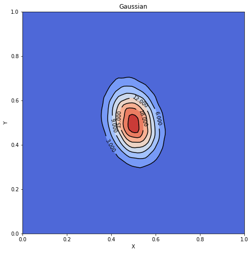
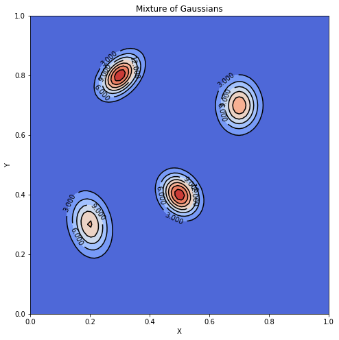
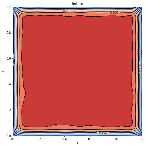
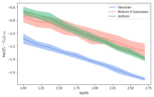
Figure 3. From left to right: densities of the sampled Gaussian, Mixture of $4$ Gaussians and Uniform distributions and sampling distance $\|T_{\mu}-T_{\mu_{N}}\|_{\mathrm{L}^{2}(\rho)}$ as a function of $N$

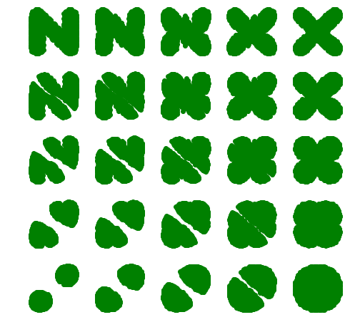
Figure 4. Barycenters of $4$ point clouds. Weights $(\lambda_{s})_{s}$ are bilinear w.r.t the corners of the square.

4.4. Barycenter approximation and clustering

Computing means and barycenters is often necessary in unsupervised learning contexts. For point cloud data, the Wasserstein distance is a natural choice to define such barycenters. For $(\mu_{s})_{s=1,\dots,S}$ $S$ discrete probability measures (corresponding to $S$ point clouds), the barycenter of $(\mu_{s})$ with non-negative weights $(\lambda_{s})_{s=1,\dots,S}$ is the solution of the following minimization problem:

$$\min_{\mu}\sum_{s=1}^{S}\lambda_{s}\mathrm{W}_{2}^{2}(\cdot,\mu_{s}).$$ (93)

This problem does not have an explicit solution, and an optimization algorithm must be run every time the weights are changed. Using transport maps from a reference measure $\rho$, it is natural to consider instead

$$\mu=\left(\sum_{s=1}^{S}\lambda_{s}T_{\mu_{s}}\right)_{\#}\rho$$ (94)

as the barycenter of the $(\mu_{s})$, and one can indeed check that the measure $\mu$ defined by this formula minimizes $\sum_{s}\lambda_{s}W^{2}_{2,\rho}(\cdot,\mu_{s}).$ We illustrate this idea with the computation of barycenters of $4$ point clouds in Figure 4. Again, in practice operations are performed on the vectorized Monge maps $\bm{T_{\mu}}$.

These barycenters are in general not equal to their Wasserstein counterparts but they seem to retain the geometric information contained in the point clouds. This idea can be used to extend unsupervised learning algorithms such as $k$-Means to family of point clouds. As a toy example, we perform a clustering on the images of the MNIST dataset [28]. We convert the $60,000$ images of the training set into point clouds of $\mathcal{X}=[0,1]^{2}$ using a simple thresholding on the pixels intensity and we compute for each point cloud its Monge map embedding. We then perform a clustering with the $k$-means++ algorithm [4] on the vectorized Monge maps, looking for $k=20$ clusters. Figure 5 shows the push-forwards of the $20$ centroids in $L^{2}(\rho,\mathbb{R}^{d})$.

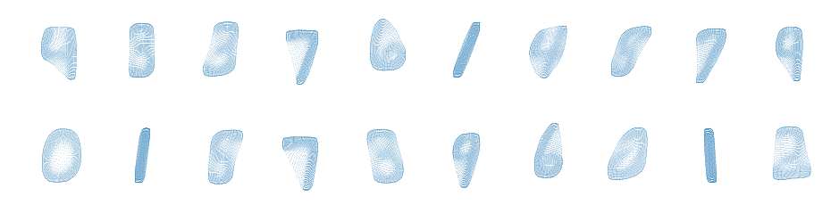
Figure 5. Push-forwards of the $20$ centroids after clustering of the Monge map embeddings of the MNIST training set.

5. CONCLUSION

We have shown that measures can readily be embedded explicitly in a Hilbert space by their optimal transport map between an arbitrary reference measure and themselves. These embeddings are shown to be injective and bi-Hölder continuous w.r.t the Wasserstein distance. They enable the definition of distances between measures and the use of generic machine learning algorithms in a computationally tractable framework.

Future work will focus on the extension of the stability theorem to more general sources and costs, to the improvement of the Hölder exponent and to statistical properties of transport plans, including concentration bounds and sample complexity of the distance they define.

Acknowledgement

The first author warmly thank Clément Cancès for pointing Lemma 3.7 in [18] and Robert Berman for discussions related to the topic of this article, and acknowledges the support of the Agence national de la recherche through the project MAGA (ANR-16-CE40-0014).

Appendix A Proof

Proof of Corollary 2.6

We first state a simple lemma that links the uniform norm of Lipschitz function to its $L^{2}(\rho)$ norm:

Lemma A.1.

If $f$ is $L$-Lipschitz on a convex bounded domain $\mathcal{X}$, then

$$\|f\|_{\infty}\leq C\|f\|_{\mathrm{L}^{2}(\mathcal{X})}^{\frac{2}{d+2}}$$ (95)

for some $C$ depending on $L$, $d$ and $\mathcal{X}$ only.

Proof of Corollary 2.6.

Theorem 2.5 implies

$$\|\nabla\psi_{\mu}-\nabla\psi_{\nu}\|^{2}_{\mathrm{L}^{2}(\mathcal{Y})}\leq C\Big{(}\int_{\mathcal{Y}}(\psi_{\nu}-\psi_{\mu})\mathrm{d}(\mu-\nu)\Big{)}^{\frac{1}{2^{d-1}}},$$ (96)

and as in Theorem 2.3, the quantity in the parenthesis can be upper bounded by $2M_{\mathcal{X}}\mathrm{W}_{1}(\mu,\nu)$. Adding a constant to $\psi_{\mu}$ if necessary, we can assume that $\int_{\mathcal{Y}}\psi_{\mu}(y)\mathrm{d}y=\int_{\mathcal{Y}}\psi_{\nu}(y)\mathrm{d}y$. The Poincaré-Wirtinger inequality on $\mathcal{Y}$ then implies

$$\|\psi_{\mu}-\psi_{\nu}\|^{2}_{\mathrm{L}^{2}(\mathcal{Y})}\leq C^{\prime}\mathrm{W}_{1}(\mu,\nu)^{\frac{1}{2^{d-1}}}$$ (97)

for some $C^{\prime}$ depending only on $\rho$, $\mathcal{X}$ and $\mathcal{Y}$.

We reuse the fact that $\psi_{\mu}-\psi_{\nu}$ is Lipschitz with constant $\leq 2M_{\mathcal{X}}$ to use Lemma A.1:

$$\|\psi_{\mu}-\psi_{\nu}\|_{\infty}\leq C\mathrm{W}_{1}(\mu,\nu)^{\frac{2}{2^{d-1}(d+2)}}.$$ (98)

Since $\phi_{\mu}=\psi_{\mu}^{*}$ and $\phi_{\nu}=\psi_{\nu}^{*}$, the definition of the Legendre transform (7) yields

$$\|\phi_{\mu}-\phi_{\nu}\|_{\infty}\leq\|\psi_{\mu}-\psi_{\nu}\|_{\infty}\leq C\mathrm{W}_{1}(\mu,\nu)^{\frac{2}{2^{d-1}(d+2)}}.$$ (99)

We conclude using Proposition 3.7 and the fact that $\phi_{\mu}$ is $\operatorname{diam}(\mathcal{Y})$-Lipschitz: there exists a constant $C$ depending only on $\rho$, $\mathcal{X}$ and $\mathcal{Y}$ such that

$$\|T_{\mu}-T_{\nu}\|_{\mathrm{L}^{2}(\rho)}\leq C\mathrm{W}_{1}(\mu,\nu)^{\frac{1}{2^{(d-1)}(d+2)}}\qed$$

Proof of Proposition 3.6

This proof is a straightforward adaptation of a stability result for finite volume discretization of elliptic PDEs, see Lemma 3.7 in [18]. We consider the function $u$ on $\mathcal{X}$ defined a.e. by $\left.u\right|_{V_{i}(\bm{\psi})}=v_{i}$. Then,

$$\langle v^{2}-\langle v|G(\bm{\psi})\rangle^{2}|G(\bm{\psi})\rangle=\int_{\mathcal{X}}u^{2}-\left(\int_{\mathcal{X}}u\right)^{2}=\frac{1}{2}\int_{\mathcal{X}\times\mathcal{X}}(u(x)-u(y))^{2}\mathrm{d}y\mathrm{d}x$$ (100)

so it suffices to control the right hand side of this equality. Given $(i,j)\in\{1,\ldots,N\}$ and $(x,y)\in X$, we denote

$$\chi_{ij}(x,y)=\begin{cases}1&\hbox{ if }V_{i}(\bm{\psi})\cap V_{j}(\bm{\psi})\cap[x,y]\neq\emptyset\hbox{ and }\langle y_{j}-y_{i}|y-x\rangle\geq 0\\ 0&\hbox{ if not.}\end{cases}$$ (101)

Then, $u(y)-u(x)=\sum_{i\neq j}(v(y_{j})-v(y_{i}))\chi_{ij}(x,y)$. We introduce

$$d_{ij}=\left\|y_{j}-y_{i}\right\|,\qquad c_{ij,z}=\left|\langle\frac{z}{\left\|z\right\|}|\frac{y_{j}-y_{i}}{\left\|y_{j}-y_{i}\right\|}\rangle\right|,$$ (102)

and we apply Cauchy-Schwarz’s inequality to get

$$(u(y)-u(x))^{2} =\left(\sum_{i\neq j}(v(y_{j})-v(y_{i}))\chi_{ij}(x,y)\right)^{2}$$

$$\leq\sum_{i\neq j}\frac{(v(y_{j})-v(y_{i}))^{2}}{d_{ij}c_{ij,y-x}}\chi_{ij}(x,y)\sum_{i\neq j}d_{ij}c_{ij,y-x}\chi_{ij}(x,y)$$ (103)

In addition, when $\chi_{ij}(x,y)=1$, we have $\langle y-x|y_{j}-y_{i}\rangle\geq 0$ so that

$$d_{ij}c_{ij,y-x}=\left\|y_{j}-y_{i}\right\|\langle\frac{y-x}{\left\|y-x\right\|}|\frac{y_{j}-y_{i}}{\left\|y_{j}-y_{i}\right\|}\rangle\geq 0$$ (104)

and

$$\sum_{i\neq j}d_{ij}c_{ij,y-x}\chi_{ij}(x,y)=\sum_{i\neq j}\langle\frac{y-x}{\left\|y-x\right\|}|y_{j}-y_{i}\rangle\chi_{ij}(x,y)\leq\operatorname{diam}(\mathcal{Y}).$$ (105)

Therefore,

$$\int_{\mathcal{X}\times\mathcal{X}}(u(y)-u(x))^{2}\mathrm{d}x\mathrm{d}y$$

$$\leq\operatorname{diam}(\mathcal{Y})\int_{\mathcal{X}\times\mathcal{X}}\sum_{i\neq j}\frac{(v(y_{j})-v(y_{i}))^{2}}{d_{ij}c_{ij,y-z}}\chi_{ij}(x,y)\mathrm{d}x\mathrm{d}y$$

$$=\operatorname{diam}(\mathcal{Y})\int_{B(0,\operatorname{diam}(\mathcal{X}))}\sum_{i\neq j}\frac{(v(y_{j})-v(y_{i}))^{2}}{d_{ij}c_{ij,z}}\left(\int_{\mathcal{X}}\chi_{ij}(x,x+z)\mathrm{d}x\right)\mathrm{d}z$$ (106)

Moreover, denoting $m_{ij}=\mathrm{vol}^{d-1}(V_{i}(\bm{\psi})\cap V_{j}(\bm{\psi}))$ we get

$$\int_{\mathcal{X}}\chi_{ij}(x,x+z)\mathrm{d}x\leq m_{ij}\left\|z\right\|c_{ij,z}$$ (107)

thus giving

$$\int_{\mathcal{X}\times\mathcal{X}}(u(y)-u(x))^{2}\mathrm{d}x\mathrm{d}y\leq C(d)\operatorname{diam}(\mathcal{Y})\operatorname{diam}(\mathcal{X})^{d+1}\sum_{i\neq j}\frac{m_{ij}}{d_{ij}}(v(y_{j})-v(y_{i}))^{2}$$ (108)

Define $H_{ij}=\frac{m_{ij}}{d_{ij}}$, $H_{ii}=-\sum_{j\neq i}H_{ij}$. Then, $\mathrm{D}G(\bm{\psi})=H$, and

$$\langle\mathrm{D}G(\bm{\psi})v|v\rangle =\sum_{i,j}H_{ij}v_{i}v_{j}$$

$$=\sum_{i}\left(H_{ii}v_{i}v_{i}+\sum_{j\neq i}H_{ij}v_{i}v_{j}\right)$$

$$=\sum_{i}\sum_{j\neq i}H_{ij}v_{i}(v_{j}-v_{i})$$

$$=\sum_{j\neq i}H_{ij}v_{i}(v_{j}-v_{i}):=A.$$ (109)

And

$$\sum_{i\neq j}H_{ij}(v(y_{j})-v(y_{i}))^{2}=\sum_{i\neq j}H_{ij}v_{j}(v_{j}-v_{i})-\sum_{i\neq j}H_{ij}v_{i}(v_{j}-v_{i})=-2A.$$ (110)

We finally obtain

$$\iint(u(y)-u(x))^{2}\mathrm{d}x\mathrm{d}y\leq-C_{d,\mathcal{X},\mathcal{Y}}\langle\mathrm{D}G(\bm{\psi})v|v\rangle.$$ (111)

References

- [1] Jean Alaux, Edouard Grave, Marco Cuturi, and Armand Joulin. Unsupervised hyperalignment for multilingual word embeddings. CoRR, abs/1811.01124, 2018.
- [2] Luigi Ambrosio, Nicola Gigli, and Giuseppe Savaré. Gradient flows: in metric spaces and in the space of probability measures. Springer Science & Business Media, 2008.
- [3] Martin Arjovsky, Soumith Chintala, and Léon Bottou. Wasserstein generative adversarial networks. In Doina Precup and Yee Whye Teh, editors, Proceedings of the 34th International Conference on Machine Learning, volume 70 of Proceedings of Machine Learning Research, pages 214–223, International Convention Centre, Sydney, Australia, 06–11 Aug 2017. PMLR.
- [4] David Arthur and Sergei Vassilvitskii. k-means++: The advantages of careful seeding. In Proceedings of the eighteenth annual ACM-SIAM Symposium on Discrete Algorithms, pages 1027–1035, 2007.
- [5] Franz Aurenhammer, Friedrich Hoffmann, and Boris Aronov. Minkowski-type theorems and least-squares clustering. Algorithmica, 20(1):61–76, 1998.
- [6] Jean-David Benamou, Guillaume Carlier, Quentin Mérigot, and Edouard Oudet. Discretization of functionals involving the monge–ampère operator. Numerische mathematik, 134(3):611–636, 2016.
- [7] Robert J. Berman. Convergence rates for discretized monge-ampère equations and quantitative stability of optimal transport. arXiv preprint 1803.00785, 2018.
- [8] Jérémie Bigot, Elsa Cazelles, and Nicolas Papadakis. Central limit theorems for entropy-regularized optimal transport on finite spaces and statistical applications. working paper or preprint, February 2019.
- [9] Yann Brenier. Polar factorization and monotone rearrangement of vector-valued functions. Communications on Pure and Applied Mathematics, 44(4):375–417, 1991.
- [10] Luis A Caffarelli, Sergey A Kochengin, and Vladimir I Oliker. Problem of reflector design with given far-field scattering data. Monge Ampère equation: applications to geometry and optimization, 226:13, 1999.
- [11] Guillermo Canas and Lorenzo Rosasco. Learning probability measures with respect to optimal transport metrics. Advances in Neural Information Processing Systems, 4, 09 2012.
- [12] Elsa Cazelles, Vivien Seguy, Jérémie Bigot, Marco Cuturi, and Nicolas Papadakis. Log-pca versus geodesic pca of histograms in the wasserstein space. SIAM Journal on Scientific Computing, 40, 08 2017.
- [13] Frédéric Chazal, David Cohen-Steiner, André Lieutier, Quentin Mérigot, and Boris Thibert. Inference of curvature using tubular neighborhoods. In Modern Approaches to Discrete Curvature, pages 133–158. Springer, 2017.
- [14] Victor Chernozhukov, Alfred Galichon, Marc Hallin, and Marc Henry. Monge–Kantorovich depth, quantiles, ranks and signs. Annals of Statistics, 45(1):223–256, 2017.
- [15] MJP Cullen, J Norbury, and RJ Purser. Generalised lagrangian solutions for atmospheric and oceanic flows. SIAM Journal on Applied Mathematics, 51(1):20–31, 1991.
- [16] Marco Cuturi. Sinkhorn distances: Lightspeed computation of optimal transport. In Proceedings of the 26th International Conference on Neural Information Processing Systems - Volume 2, NIPS’13, pages 2292–2300, 2013.
- [17] Fernando De Goes, Katherine Breeden, Victor Ostromoukhov, and Mathieu Desbrun. Blue noise through optimal transport. ACM Transactions on Graphics (TOG), 31(6):171, 2012.
- [18] Robert Eymard, Thierry Gallouët, and Raphaèle Herbin. Finite volume methods. Handbook of numerical analysis, 7:713–1018, 2000.
- [19] Rémi Flamary, Marco Cuturi, Nicolas Courty, and Alain Rakotomamonjy. Wasserstein Discriminant Analysis. Machine Learning, 107(12):1923–1945, December 2018.
- [20] Thomas P. Fletcher, Conglin Lu, Stephen M Pizer, and Sarang Joshi. Principal geodesic analysis for the study of nonlinear statistics of shape. IEEE transactions on medical imaging, 23(8):995–1005, 2004.
- [21] Wilfrid Gangbo and Robert J McCann. The geometry of optimal transportation. Acta Mathematica, 177(2):113–161, 1996.
- [22] Aude Genevay, Marco Cuturi, Gabriel Peyré, and Francis Bach. Stochastic optimization for large-scale optimal transport. In Advances in neural information processing systems, pages 3440–3448, 2016.
- [23] Aude Genevay, Gabriel Peyre, and Marco Cuturi. Learning generative models with sinkhorn divergences. In Amos Storkey and Fernando Perez-Cruz, editors, Proceedings of the Twenty-First International Conference on Artificial Intelligence and Statistics, volume 84 of Proceedings of Machine Learning Research, pages 1608–1617, Playa Blanca, Lanzarote, Canary Islands, 09–11 Apr 2018. PMLR.
- [24] Nicola Gigli. On hölder continuity-in-time of the optimal transport map towards measures along a curve. Proceedings of the Edinburgh Mathematical Society, 54(2):401–409, 2011.
- [25] Paula Gordaliza, Eustasio Del Barrio, Gamboa Fabrice, and Jean-Michel Loubes. Obtaining fairness using optimal transport theory. In Kamalika Chaudhuri and Ruslan Salakhutdinov, editors, Proceedings of the 36th International Conference on Machine Learning, volume 97 of Proceedings of Machine Learning Research, pages 2357–2365, Long Beach, California, USA, 09–15 Jun 2019. PMLR.
- [26] Jan-Christian Hütter and Philippe Rigollet. Minimax rates of estimation for smooth optimal transport maps. arXiv preprint 1905.05828, 2019.
- [27] Jun Kitagawa, Quentin Mérigot, and Boris Thibert. Convergence of a newton algorithm for semi-discrete optimal transport. Journal of the European Mathematical Society, 2019.
- [28] Yann LeCun and Corinna Cortes. MNIST handwritten digit database. 2010.
- [29] Bruno Lévy. A numerical algorithm for l2 semi-discrete optimal transport in 3d. ESAIM: Mathematical Modelling and Numerical Analysis, 49(6):1693–1715, 2015.
- [30] Quentin Mérigot. A multiscale approach to optimal transport. In Computer Graphics Forum, volume 30, pages 1583–1592. Wiley Online Library, 2011.
- [31] Ricardo H Nochetto and Wujun Zhang. Pointwise rates of convergence for the oliker–prussner method for the monge–ampère equation. Numerische Mathematik, 141(1):253–288, 2019.
- [32] Vladimir I Oliker and Laird D Prussner. On the numerical solution of the equation and its discretizations, i. Numerische Mathematik, 54(3):271–293, 1989.
- [33] Felix Otto. The geometry of dissipative evolution equations: the porous medium equation. Communications in Partial Differential Equations, 26:101–174, 2001.
- [34] Gabriel Peyré and Marco Cuturi. Computational optimal transport. Foundations and Trends in Machine Learning, 11(5-6):355–607, 2019.
- [35] Aaditya Ramdas, Nicolas Garcia, and Marco Cuturi. On wasserstein two sample testing and related families of nonparametric tests. Entropy, 19, 09 2015.
- [36] Filippo Santambrogio. Optimal transport for applied mathematicians. Birkäuser, NY, 55:58–63, 2015.
- [37] Cédric Villani. Topics in optimal transportation. American Mathematical Soc., 2003.
- [38] Wei Wang, Dejan Slepčev, Saurav Basu, John A. Ozolek, and Gustavo K. Rohde. A linear optimal transportation framework for quantifying and visualizing variations in sets of images. Int. J. Comput. Vision, 101(2):254–269, January 2013.
- [39] Jonathan Weed and Quentin Berthet. Estimation of smooth densities in wasserstein distance, 2019.