Capacity-resolution trade-off in the optimal learning of multiple low-dimensional manifolds by attractor neural networks

Abstract

Recurrent neural networks (RNN) are powerful tools to explain how attractors may emerge from noisy, high-dimensional dynamics. We study here how to learn the $\sim N^{2}$ pairwise interactions in a RNN with $N$ neurons to embed $L$ manifolds of dimension $D\ll N$. We show that the capacity, i.e. the maximal ratio $L/N$, decreases as $|\log\epsilon|^{-D}$, where $\epsilon$ is the error on the position encoded by the neural activity along each manifold. Hence, RNN are flexible memory devices capable of storing a large number of manifolds at high spatial resolution. Our results rely on a combination of analytical tools from statistical mechanics and random matrix theory, extending Gardner’s classical theory of learning to the case of patterns with strong spatial correlations.

How sensory information is encoded and processed by neuronal circuits is a central question in computational neuroscience. In many brain areas, the activity of neurons, $\sigma$, is found to depend strongly on some continuous sensory correlate $\bf r$; examples include simple cells in the V1 area of the visual cortex coding for the orientation of a bar presented to the retina, and head direction cells in the subiculum or place cells in the hippocampus, whose activities depend, respectively, on the orientation of the head and the position of an animal in the physical space. Over the past decades, Continuous Attractor (CA) neural networks have emerged as an appealing concept to explain such findings, more precisely, how a large and noisy neural population can reliably encode ‘positions’ in low-dimensional sensory manifolds, $\sigma=\Phi({\bf r})$, and continuously update their values over time according to input stimuli Amari77 ; tsodyks95 ; Benyshai95 ; Wong10 ; Zhong18 .

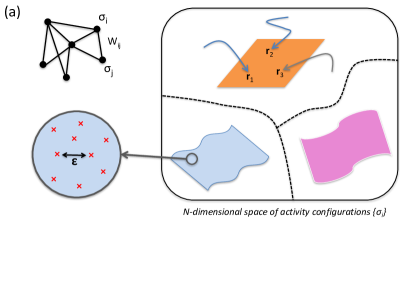
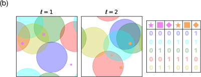
Figure 1: (a) A recurrent network with $N$ neurons and connectivity matrix ${\bf W}$ (top left) generates high-dimensional activity configurations attracted to multiple low-dimensional manifolds (right); on each manifold, we require to memorize $p$ points (bottom left, red crosses), whose separation defines the spatial resolution $\epsilon$. (b) Place fields (PF) of $N=5$ neurons in two maps, out of the three shown in panel (a). Each color identifies one neuron; the corresponding PF define the regions (with periodic boundary conditions) in the maps in which the neuron is active. The table lists, for each map, $p=3$ activity patterns corresponding to the marked points.

Models for the embedding of a CA in Recurrent Neural Network (RNN) generally assume that, after a Hebbian-like learning phase, the connection $W_{ij}$ between the neurons $i,j$ having their place fields centered in positions ${\bf r}_{i}$ and ${\bf r}_{j}$, takes value

$$W_{ij}=w\big{(}|{\bf r}_{i}-{\bf r}_{j}|\big{)}\ ,$$ (1)

where $|\cdot|$ denotes the distance in the sensory space. If $w$ is sufficiently excitatory at short distances and inhibitory at long ones, a bump state spontaneously emerges, in which active neurons tend to code for nearby positions in the sensory space. Weak external inputs suffice to move the bump and span the $D$-dimensional manifold of all possible positions $\bf r$ (Fig. 1(a)). This mechanism was observed in the ellipsoid body of the fly, where a bump of activity points towards the heading direction Kim17 . Indirect evidences for the presence of CA have been reported, e.g. in the grid-cell system Yoon13 and in the prefontal cortex Wimmer14 .

Hebbian connections (1) can be modified to embed in the same network of $N$ neurons multiple, unrelated CAs (Fig. 1(a)), such as multiple hippocampal spatial maps corresponding to different environments Alme14 or contextual situations Jezek11 . Assuming each one of the $L$ maps contributes equally to the learning process, connections take the form Samso97

$$W_{ij}=\sum_{\ell=1}^{L}w\big{(}|{\bf r}_{i}^{\ell}-{\bf r}_{j}^{\ell}|\big{)}\ ,$$ (2)

where ${\bf r}_{i}^{\ell}$ is the center of the place field (PF) of neuron $i$ in environment $\ell$ (Fig. 1(b)). Theoretical calculations show that a bump state can exist (in any map) as long as $L<\alpha_{c}\,N$, where $\alpha_{c}$ defines the critical capacity that can be sustained by the network Battaglia98 ; Monasson13 .

There are, however, serious practical and conceptual issues with the current theoretical understanding of multiple CAs based on (2). First, as soon as $L\geq 2$, the activity bump gets stuck in some preferred locations in the retrieved map due to the interferences coming from the other $L-1$ non-retrieved maps Cerasti13 . In other words, rule (2) does not define truly CAs, as large barriers oppose the motion of the bump along the map Monasson14 . The spatial error $\epsilon$ with which the environment is encoded, defined as the average discrepancy between any initial position ${\bf r}$ for the bump and the closest stable position in which it finally settles after neural relaxation dynamics, becomes quite large as $L$ increases (Fig. 2(a)). The issue of spatial resolution is also unclear from a theoretical point of view. Capacity calculations Battaglia98 ; Monasson13 require that a bump can form in any of the $L$ maps, in at least one position: they offer no guarantee about the existence of other memorized positions, and, more generally, about the value of $\epsilon$.

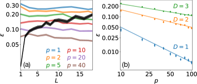
Figure 2: (a) Spatial error $\epsilon$ vs. number $L$ of two-dimensional maps in a network of $N=1000$ neurons. Black: rule (2), with $w(d)=e^{-d/.01}+w_{0}$, where $w_{0}<0$ enforces a fraction $\phi_{0}=.3$ of active cells. Colors: SVM results for different numbers $p$ of prescribed positions. Line widths show the error bars, see SM Sec. I.E for details about the calculation of $\epsilon$. (b) Spatial error $\epsilon$ vs. number $p$ of positions in a network of $N=1000$ neurons storing $L=5$ maps, in dimensions $D=1,2,3$. Lines show the expected scalings $\epsilon\sim p^{-{1}/{D}}$ in log-log scale.

Secondly, the values of the critical capacity $\alpha_{c}$ with rule (2) are generally quite low. It is reasonable to expect that the optimal storage capacity could be much higher: a $\sim 15$-fold increase was found from the Hebb-rule critical capacity, $\simeq 0.14$ AGS85 , to the optimal capacity, $\alpha_{c}=2$ Gardner88 in the case of $0$-dimensional attractors, corresponding to the Hopfield model Hopfield82 . Optimal learning could also provide detailed insights on the statistical structure of the neural couplings $W_{ij}$, which could be compared to the physiological distribution of synaptic connections Brunel16 .

In this Letter, we present a theory of optimal storage of multiple quasi-continuous maps with prescribed spatial resolution in a RNN with $N$ binary neurons ($\sigma_{i}=0,1$) and real-valued, oriented connections $W_{ij}$. A map in this context is defined through the set of the input (place) fields of the $N$ neurons, each covering a volume fraction $\phi_{0}$ of the $D$-dimensional cube (Fig. 1(b)). In practice, the centers ${\bf\hat{r}}^{\ell}_{i}$ of the PFs are uniformly drawn at random in the cube, independently of each other, in all $\ell=1...L$ maps. For each map $\ell$, we draw uniformly at random $p$ positions ${\bf\hat{r}}^{\ell,\mu}$, $\mu=1...p$, and collect the $p$ corresponding patterns of activity: the neuron $i$ is active ($\sigma^{\ell,\mu}_{i}=1$) if the distance $|{\bf\hat{r}}^{\ell,\mu}-{\bf\hat{r}}^{\ell}_{i}|$ is smaller than the PF radius $r_{c}$, and silent ($\sigma^{\ell,\mu}_{i}=0$) otherwise (Figs. 1(a)&(b)).

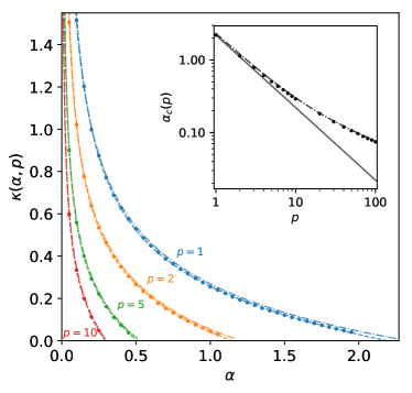
Figure 3: Optimal stability $\kappa$ as a function of the load $\alpha$ and the number $p$ of positions. Dots: SVM results; Dashed lines: Gardner’s theory (4); Dashed-dotted lines: quenched PF theory (Capacity-resolution trade-off in the optimal learning of multiple low-dimensional manifolds by attractor neural networks). Parameter values: $D=2$, $\phi_{0}=.3$, $N=1000$ for SVM. Inset: $\alpha_{c}(p)$ decreases proportionally to $1/p$ (straight line) at low $p$, and much more slowly for large $p$. Dots indicate results from SVM ($N=5000$), averaged over $50$ samples, see SM Sec. I.D for details on the estimation of $\alpha_{c}(p)$; the dot size indicates the maximal error bar. The dashed-dotted line shows the predictions from the quenched PF theory.

In order to learn these patterns we use Support Vector Machines (SVM) with linear kernels and hard margin classification (SM, Sec. I.B) SVM convex sklearn . We train $N$ SVM, one for every row $i$ in the coupling matrix $W_{ij}$, in which we consider the neuron $i$ as the output and the other $N-1$ neurons $j(\neq i)$ as the inputs Chung2018 . The training set $\{\sigma^{\ell,\mu}_{i}\}$ is common to all SVM. Once learning is complete, we normalize each row of the coupling matrix to $\sum_{j(\neq i)}W_{ij}^{2}=1$. SVM find the coupling matrix $\bf W$ maximizing the stability of the stored patterns,

$$\hskip-2.84544pt\kappa=\max_{\bf W}\min_{\{i=1...N,\ell=1...L,\mu=1...p\}}\Big{[}\big{(}2\sigma_{i}^{\ell,\mu}-1\big{)}\sum_{j(\neq i)}W_{ij}\,\sigma_{j}^{\ell,\mu}\Big{]}\ .$$ (3)

SVM couplings share some qualitative features with their Hebbian counterparts. First, the couplings $W_{ij}$ are correlated with the distances $d_{ij}^{\ell}=|{\bf r}_{i}^{\ell}-{\bf r}_{j}^{\ell}|$ between the PF centers of the neurons $i$ and $j$ in the different maps $\ell$, see SM Sec. I.C. Secondly, when simulating the trained network with simple rules for updating the neuron activities (SM, Sec. I.E), the activity bump forms and diffuses within a map, and occasionally jumps to other maps Samso97 ; Monasson14 ; Monasson15 . However, with the maximal-stability learning rule, the spatial error $\epsilon$ can be tuned at will by varying $p$, see Fig. 2(a). For a fixed $p$, $\epsilon$ remains remarkably stable as the load increases until its critical value is reached. This is in sharp contradistinction with the Hebb rule case, for which $\epsilon$ quickly increases with the number of maps. The $p$ patterns form a discrete approximation of the map, with average spatial error scaling as $\epsilon=p^{-1/D}$, i.e. as the typical distance between neighboring points (Figs. 1(a)&2(b)).

The optimal stability $\kappa$ (3) is shown in Fig. 3 as a function of the load $\alpha=L/N$ and of the number $p$ of prescribed fixed points; it is much higher than the maximal stability achievable with rule (2) after optimization over the interaction kernel $w$, see SM, Sec. I.D. As expected, $\kappa(\alpha,p)$ is a decreasing function of $\alpha$ and $p$: increasing the number of maps or enforcing finer spatial resolution reduces the stability. The value of the load at which $\kappa(\alpha,p)$ vanishes defines the critical capacity $\alpha_{c}(p)$, that is, the maximal load sustainable by the network as a function of the required spatial resolution. Figure 3(inset) shows that $\alpha_{c}(p)$ decreases proportionally to $1/p$ at low $p$, and then much more slowly as $p$ grows. For small $p$, all $L\times p$ patterns are roughly independent, and we have $\alpha_{c}(p)\simeq\frac{\alpha_{c}(1)}{p}$, where $\alpha_{c}(1)$ is the capacity of the perceptron with independent, biased patterns having a fraction $\phi_{0}$ of active neurons Gardner88 . As $p$ gets large, substantial redundancies between the $p$ patterns within a map appear, as nearby positions define similar patterns (Fig. 1(b)), and the capacity is expected to decrease less quickly with $p$. The cross-over takes place at $p_{c.o.}\sim 1/\phi_{0}$ (SM, Sec. I.D). The non-trivial behavior of $\alpha_{c}(p)$ when $p\gg p_{c.o.}$ will be characterized in the theoretical study below.

Gardner’s framework Gardner88 can, in principle, be applied to the optimal couplings corresponding to maximal stability $\kappa$ (3). Following standard calculations (SM, Sec. II.A spinglass ), we find that the maximal load at fixed $\kappa$ and $p$ is given by

$$\alpha_{c}(\kappa,p)=1/\min_{m}\;\langle E_{p}({\cal\hat{R}},{\cal Z},m;\kappa)\rangle_{{\cal\hat{R}},{\cal Z}}\ ,$$ (4)

where the minimum is taken over $m=\phi_{0}\sum_{j(\neq i)}W_{ij}$. In the formula above, $\langle\cdot\rangle$ denotes the average over the vectors ${\cal\hat{R}}=({\bf\hat{r}}_{1},...,{\bf\hat{r}}_{p})$ of $p$ positions ${\bf\hat{r}}_{\mu}$ drawn uniformly at random in the $D$-dimensional cube, and ${\cal Z}=(z_{1},...z_{p})$ drawn from the multivariate centered Gaussian distribution with ${\cal\hat{R}}$–dependent covariance matrix

$$\boldsymbol{\Gamma}_{\mu,\nu}({\cal\hat{R}})=\Gamma\big{(}|{\bf\hat{r}}_{\mu}-{\bf\hat{r}}_{\nu}|\big{)}-\phi_{0}^{2}\ .$$ (5)

Here, $\Gamma(d)$ is the overlapping volume between two PFs, whose centers are at distance $d$ from one another; hence, $\Gamma(0)=\phi_{0}$. Function $E_{p}$ in (4) is defined through

$$E_{p}({\cal\hat{R}},{\cal Z},m;\kappa)=\min_{\{t_{\mu}\geq\kappa+m,\mu=1...p\}}\sum_{\mu,\nu=1}^{p}\bigg{(}t_{\mu}-z_{\mu}-2\,m\,\Phi(|{\bf\hat{r}}_{\mu}|)\bigg{)}\,\boldsymbol{\Gamma}^{-1}_{\mu,\nu}({\cal\hat{R}})\,\bigg{(}t_{\nu}-z_{\nu}-2\,m\,\Phi(|{\bf\hat{r}}_{\nu}|)\bigg{)}\ ,$$ (6)

where $\Phi(d)=1$ if $d<r_{c}$, 0 otherwise; $r_{c}$ is the radius of the PF, i.e. the smallest number such that $\Gamma(2\,r_{c})=0$.

In practice, computing $\alpha_{c}(\kappa,p)$ from (4) is quite involved from a numerical point of view, as it requires to solve the $p$-dimensional semi-definite quadratic optimization problem in (6), as well as to average over the random vectors $\cal\hat{R}$ and $\cal Z$. This can be accurately done for small enough $p$, with results in excellent agreement with the SVM simulations, see Fig. 3. Notice that, for $p=1$, our calculation reproduces Gardner’s critical capacity $\alpha_{c}(1)$ for independent and biased patterns (SM, Sec. II.B). This is expected as spatial correlations between patterns within a map appear when $p\geq 2$.

Formula (4) seems, unfortunately, intractable for large $p$. The intricate dependence on $p$, e.g. showing up through the Gaussian correlations between the $p$ random fields $z_{\mu}$ in (6), stems from the average (in each map $\ell$) over the $N$ PF centers, $\{{\bf r}_{i}^{\ell}\}$, at fixed positions $\{{\bf r}^{\ell,\mu}\}$. To avoid introducing these correlations and have an explicit dependence on the parameter $p$, we consider an alternative calculation scheme, where the $p$ positions in each map are averaged out, while keeping the $L\times N$ centers quenched. To further simplify the calculation we neglect in the effective action all terms of order $\geq 3$ in the couplings $W_{ij}$ Monasson93 ; this Gaussian approximation is expected to be exact in the large-$p$ limit. Details about the calculation can be found in SM, Sec. II.C. Within our quenched PF theory the optimal load $\alpha_{c}(\kappa,p)$ is the root of $F$ defined through

$$F(\alpha;m,q,U,V,T) = V\bigg{(}q+U-\frac{m^{2}}{1-\frac{4}{g(U)}+4U}\bigg{)}$$

$$\hskip-103.28363pt+T\bigg{(}1+\frac{U\,g(U)-1}{V}\bigg{)}-\alpha p(q-m^{2})\int_{x}^{\infty}dz\,\frac{e^{-\frac{z^{2}}{2}}}{\sqrt{2\pi}}(z-x)^{2}$$

with $x=\frac{m-\kappa}{\sqrt{q-m^{2}}}$. In (Capacity-resolution trade-off in the optimal learning of multiple low-dimensional manifolds by attractor neural networks), $m=\sum_{j(\neq i)}(2\,\boldsymbol{\cal C}_{ij}-\phi_{0})W_{ij}$, $q=\sum_{j,k(\neq i)}W_{ij}\boldsymbol{\cal C}_{jk}W_{ik}$, and the Lagrange multipliers $U,V,T$ enforcing, respectively, the normalization of $W$ and the definition of the order parameters, are all chosen to optimize $F$. $\boldsymbol{\cal C}$ denotes the $N\times N$ multi-space Euclidean Random Matrix (ERM)

$$\boldsymbol{\cal C}_{jk}\big{(}\{{\bf r}_{i}^{\ell}\}\big{)}=\frac{1}{L}\sum_{\ell=1}^{L}\Gamma\big{(}|{\bf r}_{j}^{\ell}-{\bf r}_{k}^{\ell}|\big{)}\ ,$$ (8)

with resolvent $g(U)=\frac{1}{N}\text{Trace}\,(U\,{\bf Id}+\boldsymbol{\cal C})^{-1}$. While ERM have been intensively studied in the literature ERM , superimpositions of ERM mixing up different spaces have not been considered so far to our knowledge. The resolvent $g(U)$ can nevertheless be computed using tools from Random Matrix Theory vivo Battista19 , and shown to be solution of the implicit equation

$$U=\frac{1}{g(U)}-\sum_{{\bf k}\neq{\bf 0}}\frac{\alpha\,\hat{\Gamma}({\bf k})}{\alpha+g(U)\,\hat{\Gamma}({\bf k})}\ ,$$ (9)

where the $\hat{\Gamma}({\bf k})$’s are the components of the Fourier transform of $\Gamma$ on the $D$-dimensional infinite reciprocal cube.

Resolution of these equations gives access to $\kappa(\alpha,p)$, in very good agreement with the numerical results obtained with SVM (Fig. 3). Small deviations can, however, be noticed and diminish with increasing $p$ as expected. The order parameters $q$ and $m$ are shown as functions of $p$ in Fig. 4, in good agreement with SVM results for large $p\ (\gg p_{c.o.})$. The value of $p$ at which the confluence between the results from the quenched theory and SVM takes place is a decreasing function of the PF size $\phi_{0}$ (SM, Sec. II.D mizuseki hussaini ) and of the map dimension $D$ (SM, Sec. I.D).

Due to the explicit dependence of $F$ on $p$ in (Capacity-resolution trade-off in the optimal learning of multiple low-dimensional manifolds by attractor neural networks) the asymptotic behaviour of the critical capacity can be analytically determined in the large–$p$ limit:

$$\alpha_{c}(p)\sim A(D)\;\frac{\phi_{0}^{-(D-1)}}{(\log p)^{D}}\qquad(p\to\infty)\ ,$$ (10)

where the constant $A$ is made explicit in SM, Sec. II.C. Equation (10) is our main result. Informally speaking, the very slow decay of the critical capacity with $p$ (Fig. 3, inset) means that recurrent neural nets can efficiently store multiple spatial maps, even at high spatial resolution. More precisely, enforcing a strong reduction of the spatial error, such as $\epsilon\to\epsilon^{2}$, results in a moderate drop of the maximal sustainable load, $\alpha_{c}\to\alpha_{c}/2^{D}$. In addition, the capacity is predicted to be a decreasing function of the PF size in dimensions $D=2,3$, but not in dimension $D=1$. This asymptotic statement is qualitatively corroborated by SVM results, even for moderate values of $p$ (SM, Sec. I.D).

Figure 4: Order parameters $m$ (left) and $q$ (right) vs. $p$. Dots: SVM results ($N=2500$), averaged over $50$ samples; Dashed-dotted lines: quenched PF theory (Capacity-resolution trade-off in the optimal learning of multiple low-dimensional manifolds by attractor neural networks). Parameters: $D=2$, $\phi_{0}=.3$, $\alpha=.02$ (top) and $.05$ (bottom), for which up to, respectively, $p_{c}\simeq 2500$ and $p_{c}\simeq 250$ points can be memorized.

Many extensions of the current work can be contemplated. First, our theory can be easily generalized to the case of spatial resolutions varying from map to map, by substituting $p$ with its average value over the maps in (10). This suggests that the fraction of maps with finest spatial resolution $\epsilon$ should not exceed $\sim\epsilon^{D}$ when $\epsilon\to 0$, in order not to affect too much the critical capacity.

Secondly, it would be very interesting to understand how much the scaling of $\alpha_{c}$ in (10) is robust against the choice of the parametrization $\Phi({\bf r})$ of the manifolds. We have shown that reducing the number of active neurons in each map and allowing for variations in the sizes of the PFs from neuron to neuron do not affect this scaling Battista19 . While we have assumed here for the sake of simplicity that the distribution of points was statistically uniform across space, this need not be the case in practice. Experiments have shown that spatial representations of environments are enriched in place fields close to spots of interests (such as water pots Hollup01 or objects Bourboulou2019 ) with respect to void regions. Numerical simulations reported in SM, Sec. I.D&E show that increasing the density of prescribed positions in regions of the physical space allows us to carve specific attractors in the neural activity space, representing preferentially those regions. This result is compatible with recent studies establishing the link between PF distribution and behavioral place preference Mamad17 . Interestingly, our quenched PF theory can be applied to any particular set of PF, not necessarily homogeneously distributed over space; knowledge of the PF characteristics, e.g. from experimental measurements, allows us to determine the multispace correlation matrix $\boldsymbol{\cal C}$ in (8) and to make specific predictions. A proof of principle of this approach is shown in SM, Sec. II.D, where we compare the couplings found with SVM and with our quenched PF theory on synthetic data.

Thirdly, the biological implications of our work remain to be worked out. Several improvements should be first brought in terms of biological plausibility. In particular one should consider continuous rather than binary neurons, explicitly distinguish excitatory and inhibitory neurons and impose Dale’s law on the associated synapses, and take into account the sparse nature of synapses Guzman and of place-cell activity Alme14 observed in CA3. Border effects, known to be important for hippocampal maps Barry06 , should also be considered instead of the simple periodic boundary conditions assumed here. Finally, it would be very interesting to study the dynamics of learning. As a preliminary attempt, we consider in SM, Sec. I.F, an on-line version of the SVM learning algorithm adatron , and show that the number of presentations of the patterns needed to stabilize a map is approximately proportional to $p$. Studying plausible learning rules could ultimately elucidate how the network progressively maturates to account for more and more fixed points and eventually defines a quasi-continuous attractor, as seems to be the case during the first weeks of development in rodents Dragoi .

Acknowledgements. We are grateful to A. Treves for useful discussions. This work was funded by the HFSP RGP0057/2016 project.

References

- (1) S. Amari. Bio. Cyber. 27, 77-87 (1977)
- (2) M. Tsodyks, T. Sejnowski, Int. J. Neur. Syst. 6, 81-86 (1995)
- (3) B. Ben-Yishai, R. Bar-Or, H. Sompolinsky. Proc. Natl. Acad. Sci. 92, 3844-48 (1995)
- (4) C.C.A. Fung, K.Y.M. Wong, S. Wu, Neural Comp. 22, 752-92 (2010)
- (5) W. Zhong et al., arXiv:1809.11167 (2018)
- (6) S.S. Kim et al, Science 356, 849-853 (2017)
- (7) K. Yoon et al, Nature Neurosci. 16, 1077 (2013)
- (8) K. Wimmer et al, Nature Neurosci. 17, 431 (2014)
- (9) C.B. Alme et al, Proc. Natl. Acad. Sci. 111, 18428-35 (2014)
- (10) K. Jezek et al, Nature 478, 246 (2011)
- (11) A. Samsonovich, B.L. McNaughton, J. Neurosci. 17, 5900 (1997)
- (12) F.P. Battaglia, A. Treves. Phys. Rev. E 58, 7738 (1998)
- (13) R. Monasson, S. Rosay. Phys. Rev. E 87, 062813 (2013)
- (14) E. Cerasti, A. Treves. Front. Cell. Neurosci. 7, 112 (2013)
- (15) R. Monasson, S. Rosay. Phys. Rev. E 89, 032803 (2014)
- (16) R. Monasson, S. Rosay. Phys. Rev. Lett. 115, 098101 (2015)
- (17) D. Amit, H. Gutfreund, H. Sompolinsky. Phys. Rev. Lett. 55, 1530 (1985)
- (18) E. Gardner. J. Phys. A 21, 257 (1988).
- (19) M. Mézard, G. Parisi, M. Virasoro. Spin glass theory and beyond: An Introduction to the Replica Method and Its Applications. World Scientific Publishing Company (1987)
- (20) J.J. Hopfield, Proc. Nat. Acad. Sci. 79, 2554-58 (1982)
- (21) N. Brunel. Nature Neurosci. 19, 749 (2016)
- (22) B. Scholkopf, A.J. Smola. Learning with kernels: support vector machines, regularization, optimization, and beyond. MIT Press (2001)
- (23) S. Diamond, S. Boyd. JMLR 17, 2909-2913 (2016)
- (24) F. Pedregosa et al, JMLR 12, 2825-2830 (2011)
- (25) The case of hetero-associative classification of manifolds was recently studied by S.Y. Chung, D.D. Lee, H. Sompolinsky, Phys. Rev. X 8, 031003 (2018)
- (26) R. Monasson, J. Physique I 3, 1141-52 (1993)
- (27) A. Goetschy, S.E. Skipetrov, arXiv:1303.2880 (2013)
- (28) G. Livan, M. Novaes, P. Vivo. Introduction to random matrices: theory and practice. Springer International Publishing (2018)
- (29) A. Battista, R. Monasson, On the spectrum of multi-space Euclidean random matrices, in preparation (2019)
- (30) S.A. Hollup et al. J. Neurosci. 21, 1635-44 (2001)
- (31) R. Bourboulou et al., eLife 8:e44487 (2019)
- (32) O. Mamad et al, PLoS Biology 15: e2002365 (2017)
- (33) S.J. Guzman et al. Science 353, 1117-23 (2016)
- (34) C. Barry et al. Reviews in the Neurosciences 17, 71-97 (2006)
- (35) U. Farooq, G. Dragoi, Science 363, 168-173 (2019)
- (36) J. K. Anlauf, M. Biehl, EPL 10, 687 (1989)
- (37) K. Mizuseki et al., Hippocampus 22, 1659-1680 (2012)
- (38) S.A. Hussaini et al., Neuron 72, 643-653 (2011)