Multiple normalized standing-waves solutions to the scalar non-linear Klein-Gordon equation with two competing powers

Abstract.

In this work we prove the existence of standing-wave solutions to the scalar non-linear Klein-Gordon equation in dimension one and the stability of the ground-state, the set which contains all the minima of the energy constrained to the manifold of the states sharing a fixed charge. For non-linearities which are combinations of two competing powers we prove that standing-waves in the ground-state are orbitally stable. We also show the existence of a degenerate minimum and the existence of two positive and radially symmetric minima having the same charge.

Daniele Garrisi

Room 324, Sir Peter Mansfield Building

School of Mathematical Sciences

University of Nottingham Ningbo China

199 Taikang East Road

315100, Ningbo, China

1. Introduction

In this work we address the problem of existence and stability of standing-wave solutions to a non-linear Klein-Gordon equation

(1) $$(\partial_{tt}^{2}-\partial_{xx}^{2}+m^{2})\phi+G^{\prime}(|\phi|)\cdot\frac{\phi}{|\phi|}=0$$

where $G$ is a real-valued even function defined on $(-\infty,+\infty)$ such that $G^{\prime}(0)=0$. A standing-wave is a solution to (1) which can be written as

(2) $$\phi(t,x):=e^{-i\omega t}R(x),\quad(t,x)\in\mathbb{R}\times\mathbb{R}$$

where $\omega$ is a real number and $R$ is a real-valued function of class $H^{1}(\mathbb{R};\mathbb{R})$. The standing-waves we are interested on satisfy the following variational characterization: they are minima of the energy functional ${E}$ on the constraint $M_{\sigma}$ which depends on a real parameter $\sigma$. We set $\mathbf{X}:=H^{1}(\mathbb{R};\mathbb{C})\times L^{2}(\mathbb{R};\mathbb{C})$. For the vectors of this space we will use the notation $\Phi$, and $(\phi,\phi_{t})$ for its components. The energy and constraint functional are complex-valued functions defined on $\mathbf{X}$. Given $(\phi,\phi_{t})$ in $\mathbf{X}$, we define

(3) $${E}(\phi,\phi_{t}):=\frac{1}{2}\int_{-\infty}^{+\infty}|\phi_{t}(x)|^{2}dx+\frac{1}{2}\int_{-\infty}^{+\infty}|\phi^{\prime}(x)|^{2}dx+\int_{-\infty}^{+\infty}W(\phi(x))dx$$

(4) $$C(\phi,\phi_{t}):=-\mathrm{Im}\int_{-\infty}^{+\infty}\phi_{t}(x)\overline{\phi(x)}dx,$$

where

(5) $$W(z):=\frac{1}{2}m^{2}|z|^{2}+G(|z|).$$

In fact, ${E}$ is a real-valued functional. We will refer to $C$ with the term charge. The constraint set is defined as

$$M_{\sigma}:=\{(\phi,\phi_{t})\in\mathbf{X}\mid C(\phi,\phi_{t})=\sigma\}\subseteq\mathbf{X}.$$

Given two vectors $\Phi=(\phi,\phi_{t})$ and $\Psi=(\psi,\psi_{t})$ in $\mathbf{X}$, we consider the scalar product

$$(\Phi,\Psi)_{\mathbf{X}}:=\text{Re}\int_{-\infty}^{+\infty}\phi\overline{\psi}dx+\text{Re}\int_{-\infty}^{+\infty}\phi_{t}\overline{\psi_{t}}dx.$$

On $\mathbf{X}$ we consider the metric $d$ induced by the scalar product. In order to define stable subsets of $\mathbf{X}$, we assume that $G$ is such that (1) is globally well-posed as meant in [36, Remark 3.5, p. 126]. That is, given an initial datum $(\phi_{0},\phi_{t,0})$ in $H^{1}\times L^{2}$, there exist a unique solution $\phi$ defined on $(-\infty,+\infty)\times\mathbb{R}$ such that

(6) $$\phi\in C_{t}^{0}H^{1}_{x}((-\infty,+\infty)\times\mathbb{R})\cap C^{1}_{t}L^{2}_{x}((-\infty,+\infty)\times\mathbb{R}).$$

Moreover, ${E}$ and $C$ are constant on the trajectory $(\phi(t,\cdot),\partial_{t}\phi(t,\cdot))$, that is

(7) $${E}(\phi(t,\cdot),\partial_{t}\phi(t,\cdot))={E}(\phi_{0},\phi_{t,0}),\quad C(\phi(t,\cdot),\partial_{t}\phi(t,\cdot))=C(\phi_{0},\phi_{t,0})$$

for every $t$ in $(-\infty,+\infty)$, [36, Remark 3.5, p. 126]. Then for every $t$ in $(-\infty,+\infty)$ we can define

$$U(t,\cdot)\colon\mathbf{X}\to\mathbf{X},\quad U(t,(\phi_{0},\phi_{t,0}))=(\phi(t,\cdot),\partial_{t}\phi(t,\cdot)).$$

Definition (Stable subsets of $\mathbf{X}$).

A set $S\subseteq\mathbf{X}$ is stable if, for every $\varepsilon>0$, there exist $\delta>0$ such that

$$\mathrm{dist}(\Phi,S)<\delta\Rightarrow\mathrm{dist}(U(t,\Phi),S)<\varepsilon$$

for every $t$ in $(-\infty,+\infty)$ and $\Phi\in\mathbf{X}$.

In this work we present two stability results. The first is the stability of the subset of $\mathbf{X}$ called ground state, which is the set of all the minima of ${E}$ on the constraint $M_{\sigma}$. We use the notation

$$\Gamma_{\sigma}:=\{(\phi,\phi_{t})\in M_{\sigma}\mid{E}(\phi,\phi_{t})=\inf_{M_{\sigma}}({E})\}.$$

The literature is rich of stability results to a variety of differential equations and coupled differential equations, where the ground state is defined according to the energy functional and constraint. Since similar techniques are also used, it is covenient to mention results of stability in differential equations having different structure than (1). Some references are [4, 35] for the non-linear Schrödinger equation (NLS) in dimension $n\geq 3$, or [11] on the stability of (NLS) in dimension $n\geq 1$, [3] on the non-linear Klein-Gordon equation (NLKG) in dimension $n\geq 3$, [14] on the coupled non-linear Klein-Gordon (2-NLKG) equation in dimension $n\geq 3$, [16, 28, 19] and [32] on the coupled non-linear Schrödinger equation (2-NLS) in dimension $n=1$. We include [29, 30, 31] which address problems of stability for the non-linear Schrödinger equation in bounded domains. For the stability of the ground state we require the following assumptions:

(G1) $$\mu:=\inf_{s\in(0,+\infty)}\frac{W(s)}{s^{2}}>0$$

there exist $s_{0}>0$ such that

(G2) $$G(s_{0})<0$$

there exist $2<p<q$ such that

(G3) $$|G^{\prime}(s)|\leq C(|s|^{p-1}+|s|^{q-1}),\quad G(0)=0.$$

(G4). The equation (1) is globally well-posed in $H^{1}(\mathbb{R};\mathbb{C})\times L^{2}(\mathbb{R};\mathbb{C})$.

Theorem 1.

If (G1-G4) hold, there exist $\sigma_{*}>0$ such that $\Gamma_{\sigma}$ is stable for every $\sigma>\sigma_{*}$.

We prove the Concentration-Compactness property of the minimizing sequences of ${E}$ on $M_{\sigma}$. That is, given a minimizing sequence $(\phi_{n},\phi_{n,t})$, there exist $(y_{n})\subseteq\mathbb{R}$ such that a subsequence of $(\phi_{n}(\cdot+y_{n}),\phi_{n,t}(\cdot+y_{n}))$ converges strongly in $\mathbf{X}$. In previous references as [3, 14], the Concentration-Compactness had been proved for particular minimizing sequences, which are the ones satisfying $\phi_{n,t}=-i\omega_{n}\phi_{n}$ for some $\omega_{n}$ in $\mathbb{R}$. Equivalently, that implies the Concentration-Compactness property of the minimizing sequences of the functional $E^{*}$ and constraint $M^{*}_{\sigma}$ defined as follows:

(8) $$E^{*}\colon H^{1}(\mathbb{R};\mathbb{R})\times\mathbb{R}\to\mathbb{R},\quad C^{*}\colon H^{1}(\mathbb{R};\mathbb{R})\times\mathbb{R}\to\mathbb{R}$$

(9) $$E^{*}(u,\omega):={E}(u,-i\omega u)=\frac{1}{2}\int_{-\infty}^{+\infty}\Big{(}|u^{\prime}(x)|^{2}+\omega^{2}|u(x)|^{2}+2W(u(x))\Big{)}dx$$

(10) $$C^{*}(u,\omega)=C(u,-i\omega u)=\omega\int_{-\infty}^{+\infty}|u(x)|^{2}dx$$

and

$$M^{*}_{\sigma}:=\{(u,\omega)\in H^{1}(\mathbb{R};\mathbb{R})\times\mathbb{R}\mid C^{*}(u,\omega)=\sigma\}.$$

We address specifically the dimension $n=1$, a case which was not covered in [3, 14]. This presents different challenges. In fact, when $n\geq 3$, the functional $E^{*}$ is coercive, provided $q\leq\frac{2n}{n-2}$ in (G3) and $W\geq 0$. As we will show in Remark 2.1, in dimension $n=1$, the coercivity fails if $W\geq 0$ and $W$ has a zero different than the origin, no matter what restriction one sets on $q$. The second stability result is about the subset of $\mathbf{X}$ which is obtained by taking all the argument translations and multiplication by complex numbers in the unit sphere of an element of the ground state: given $\Phi$ in $\Gamma_{\sigma}$, we set

(11) $$\Gamma(\Phi):=\{z\Phi(\cdot+y)\mid(z,y)\in S^{1}\times\mathbb{R}\}.$$

The invariances

(12) $${E}(z\Phi(\cdot+y))={E}(\Phi),\quad C(z\Phi(\cdot+y))=C(\Phi)$$

for every $(z,y)$ in $S^{1}\times\mathbb{R}$ and $\Phi$ in $\mathbf{X}$ show that $\Gamma(\Phi)$ is a subset of $\Gamma_{\sigma}$. This result addresses specifically the double power non-linearity

(13) $$G(s)=-as^{4}+bs^{6},\quad a,b>0.$$

Definition (Orbitally stable standing wave).

The standing-wave in (2) is orbitally stable if $\Gamma(R,-i\omega R)$ is a stable subset of $\mathbf{X}$.

References on the orbital stability of $\Gamma_{\sigma}$ do not always address the set (11). In [4, 3, 14] and [16], only the stability of the ground state has been proved. Other references who proved the stability of the standing-wave took advantage of more specific assumptions. For instance, in [11] the non-linearity $G$ is a pure-power

(14) $$G(s)=-a|s|^{p},\quad a>0,\quad 2<p<2+\frac{4}{n}.$$

In [32, 28, 25, 12] the non-linearity $G$ is an homogeneous two or more variables function or fourth degree homogeneous polynomial. This choice allows to prove that $\Gamma(\Phi)=\Gamma_{\sigma}$ for every $\Phi$ element of the ground-state. Therefore, the stability of $\Gamma(\Phi)$ follows from the stability of the ground-state, that is from Concentration-Compactness property of minimizing sequences which follows by [23, 24]. Such equality is consequence of the uniqueness of positive, decaying and symmetrically decreasing solutions to the elliptic problem $\Delta R(x)-G^{\prime}(R(x))-R(x)=0$, [27, 20, 26], and the symmetry $G(ts)=t^{p}G(s)\ (t>0)$. In fact, one can show that each set $\Gamma(\Phi)$ contains a unique minimum $R$ which is positive, even, radially decreasing and $H^{1}(\mathbb{R};\mathbb{R})$. This follows, for instance, from the conclusions of [10]. We included a proof in Theorem 2. Therefore, it is convenient to define

(15) $$K_{\sigma}:=\Gamma_{\sigma}\cap H^{1}_{r,+}(\mathbb{R};\mathbb{R}),$$

where $H^{1}_{r,+}(\mathbb{R};\mathbb{R})$ is the set of $H^{1}$ positive and even functions. The choice of the powers 4 and 6 is in part motivated by historical reasons: in dimension $n=3$, the non-linear Klein-Gordon with two competing powers (13) was proposed in [21] as a model of 0-spin particles in spin theory. In [17, 18, 33, 34] they proved existence of stable and unstable standing-waves, still in dimension $n=3$. Moreover, in (13) we are able to evaluate explicitly the energy ${E}$ and the charge $C$ of the standing-wave (3), to prove the stability of $\Gamma(R,-i\omega R)$ and to count the number of minima and detect which ones are non-degenerate. In order to describe these results, we introduce the notation:

(16) $$\tau(a,b,m):=\frac{2m^{2}b}{a^{2}}.$$

The behaviour of the number of sets $\Gamma(\Phi)$ and the non-degeneracy of minima depend jointly on the non-linearity (13) and $m$ (specifically on $\tau(a,b,m)$), and $\sigma$. We list some of the main results: there exist $\tau_{*}>1$ such that

1. If $\tau\geq\tau_{*}$, then $|K_{\sigma}|=1$ for every $\sigma>0$. Therefore, in every constraint there is exactly one positive, symmetric minimum from Theorem 4. Therefore, $\Gamma_{\sigma}=\Gamma(\Phi)$ for every $\Phi$ in $\Gamma_{\sigma}$ just as it happens for pure-powers or double powers in the non-linear Schrödinger equation in [11, 13]

2. if $\tau=\tau_{*}$ there exist exactly one level $\sigma_{d}$ where the minimum is degenerate, from Theorem 5. This is a completely different behaviour than (NLS), where for double powers minima are non-degenerate, [13]. Yet the corresponding standing-wave is stable

3. if $1<\tau<\tau_{*}$, there exist exactly one level $\sigma_{2}$ where we can observe the existence of two positive, symmetrically decreasing minima, that is $|K_{\sigma}|=2$, Theorem 4. Consequently we have the disjoint union $\Gamma_{\sigma}=\Gamma(\Phi_{1})\cup\Gamma(\Phi_{2})$. This is the most unexpected result. In [7] the author proved that if $\sigma$ is large enough, one can expect to find at least as many local minima as the number of connected components of the set $\{G<0\}$. According Theorem 4, there are more local minima (in fact, minima) than the number of connected components. In fact for $G$ in (13), the set is connected. In (2-NLS) one can find more multiplicity results, as [2], even if critical points are not minima

4. the set $\Gamma(\Phi)$ is stable for every choice of $\tau>1$ and $\sigma$, Theorem 6. This applies in particular to the case where there is a unique set $\Gamma(\Phi)$, but also in the case where there are two minima and, consequently, there are two different sets $\Gamma(\Phi_{1})$ and $\Gamma(\Phi_{2})$ disjoint from each other. In [14] we already pointed out methods to prove the stability of $\Gamma(\Phi)$ regardless of the cardinality of $K_{\sigma}$. This is a concrete example showing that the uniqueness of $\Gamma(\Phi)$ is not necessary.

The paper is organized as follows. In §2 we prove properties of the pairs $({E},M_{\sigma})$ and $(E^{*},M_{\sigma}^{*})$ and the stability of the ground-state. In §3, we count the number of positive and radially decreasing minima in every constraint $M_{\sigma}$, the cardinality of $K_{\sigma}$. The result is summarized and proved in Theorem 4. In §4, we look at the degeneracy of minima through Theorem 5. The paper concludes with Theorem 6 of §5, where we prove that all the standing-waves in (3) such that $(R,-i\omega R)$ is in $\Gamma_{\sigma}$ are orbitally stable.

Throughout all the work it is assumed that $\sigma>0$. Theorems 4, 5 and 6 can be proved in the case $\sigma<0$ by observing that the isometry from $M_{\sigma}$ to $M_{-\sigma}$ which maps $(\phi,\phi_{t})$ to $(\phi,-\phi_{t})$, does not change the energy ${E}$. The case $\sigma=0$ has been addressed separately at the end of §5.

2. Properties of the functional ${E}$

Some of the properties we are going to prove have a correspondence with the variational setting of the non-linear Schrödinger equation, treated in [4]. Therefore, it is convenient to introduce a notation for the functional

(17) $${E}_{S}(\phi):=\frac{1}{2}\int_{-\infty}^{+\infty}|\phi^{\prime}(x)|^{2}+\int_{-\infty}^{+\infty}G(|\phi(x)|)dx$$

and the constraint

$$S(\lambda):=\{u\in H^{1}(\mathbb{R};\mathbb{C})\mid\|u\|_{L^{2}}^{2}=\lambda\}.$$

The functionals ${E}$ and $E^{*}$, defined in (3) and (9) can be related to each other through the following map

(18) $$P\colon\mathbf{X}\to H^{1}(\mathbb{R};\mathbb{R})\times\mathbb{R},\quad P(\phi,\phi_{t}):=\left(|\phi|,\frac{\sigma}{\|\phi\|_{L^{2}}^{2}}\right)$$

which is the one given in [3, (3.19)]. Under the assumptions (G1-G3), we can prove the following proposition.

Proposition 1.

The functional ${E}$ satisfies the following properties:

1. $E^{*}(P(\Phi))\leq{E}(\Phi)$ and $C^{*}(P(\Phi))=C(\Phi)$ for every $\Phi$ in $\mathbf{X}$

2. ${E}\geq 0$ on $M_{\sigma}$. Then it is bounded from below on $M_{\sigma}$

3. there exist a continuous real valued function $h_{1}$ such that $h_{1}(0)=0$ and for every $e$ in $\mathbb{R}$

   $${E}(\Phi)\leq e\implies\|\Phi\|_{X}\leq h_{1}(e)$$

   for every $\Phi$ in $M_{\sigma}$ and

   $$E^{*}(u,\omega)\leq e\implies\|u\|_{H^{1}}\leq h_{1}(e)$$

   for every $(u,\omega)$ in $M_{\sigma}^{*}$

4. there exist a continuous function $h_{2}$ from $\mathbb{R}\times\mathbb{R}\times\mathbf{X}$ to $\mathbb{R}$ which is bounded on bounded subsets and such that

   $$|{E}(\lambda\Phi)-{E}(\mu\Phi)|\leq h_{2}(\lambda,\mu,\Phi)|\lambda-\mu|$$

   for every triple $(\lambda,\mu,\Phi)$ in $\mathbb{R}\times\mathbb{R}\times\mathbf{X}$

5. ${E}$ and $C$ are continuously differentiable.

Proof.

(i). This property has been already thoroughly proved in [3, Lemma 3.3]. Here we add some intermediate inequalities. We set

$$\omega:=\frac{C(\Phi)}{\|\phi\|_{L^{2}}^{2}}.$$

Then, from (18), $P(\Phi)=(|\phi|,\omega)$.

(19) $$\begin{split}{E}(\phi,\phi_{t})&=\frac{1}{2}\int_{-\infty}^{+\infty}|\phi_{t}(x)|^{2}dx+\frac{1}{2}\int_{-\infty}^{+\infty}\Big{(}|\phi^{\prime}(x)|^{2}+2W(\phi(x))\Big{)}dx\\ &\geq\frac{1}{2}\int_{-\infty}^{+\infty}\Big{(}||\phi|^{\prime}(x)|^{2}+2W(\phi(x))\Big{)}dx+\frac{1}{2}\cdot\frac{|C(\Phi)|^{2}}{\|\phi\|_{L^{2}}^{2}}\\ &=\frac{1}{2}\int_{-\infty}^{+\infty}\Big{(}||\phi|^{\prime}(x)|^{2}+2W(|\phi(x)|)\Big{)}dx+\frac{1}{2}\omega^{2}\|\phi\|_{L^{2}}^{2}\\ &=E^{*}(|\phi|,\omega)=E^{*}(P(\Phi)).\end{split}$$

The second inequality follows from [22, Theorem 7.8, p., 177], the Convex Inequality for the gradient, and the Cauchy-Schwarz inequality applied to the scalar product

$$(f,g)_{L^{2}}:=\mathrm{Re}\int_{-\infty}^{+\infty}f(x)\overline{g}(x)dx,\quad f=i\phi,\quad g=\phi_{t}.$$

(ii). From (G1), it follows that $W\geq 0$. Then ${E}(\Phi)\geq 0$ for every $\Phi$ in $\mathbf{X}$.

(iii). We set $\Phi=(\phi,\phi_{t})$. Again, from (G1), we have

$$2e\geq 2{E}\geq\|\phi_{t}\|_{L^{2}}^{2}+\|\phi^{\prime}\|_{{L^{2}}^{2}}+\mu\|\phi\|_{{L^{2}}^{2}}\geq\min\{\mu,1\}\|\Phi\|_{{\mathbf{X}}^{2}}.$$

Then we can define

$$h_{1}(e):=\left(\frac{2e}{\min\{\mu,1\}}\right)^{\frac{1}{2}}.$$

Given $(u,\omega)$ in $M_{\sigma}^{*}$ if $E^{*}(u,\omega)\leq e$, then ${E}(u,-i\omega u)\leq e$ by (9). Then

$$\|u\|_{H^{1}}\leq\|(u,-i\omega u)\|_{X}\leq h_{1}(e).$$

(iv). We can write

(20) $$\begin{split}|{E}(\lambda\Phi)-{E}(\mu\Phi)|&\leq\frac{1}{2}|\lambda^{2}-\mu^{2}|\int_{-\infty}^{+\infty}|\phi_{t}(x)|^{2}dx\\ &+\frac{m^{2}}{2}|\lambda^{2}-\mu^{2}|\int_{-\infty}^{+\infty}|\phi(x)|^{2}dx\\ &+\int_{-\infty}^{+\infty}|{E}_{S}(\lambda\phi(x))-{E}_{S}(\mu\phi(x))|dx.\end{split}$$

From (ii) of [13, Proposition 1], there exist a real-valued function $c$ defined on the set $\mathbb{R}\times\mathbb{R}\times H^{1}(\mathbb{R};\mathbb{C})$ which is bounded on bounded sets and such that

(21) $$|{E}_{S}(\lambda\phi)-{E}_{S}(\mu\phi)|\leq|\lambda-\mu|c(\lambda,\mu,\phi).$$

In order to apply the quoted proposition, we only need to check that $G$ fulfills the property [13, (G2a)], which corresponds to (G2). From (20) and (21), we obtain

$$\begin{split}|{E}(\lambda\Phi)-{E}(\mu\Phi)|\leq&\frac{1}{2}|\lambda^{2}-\mu^{2}|\|\phi_{t}\|_{{L^{2}}^{2}}+\frac{m^{2}}{2}|\lambda^{2}-\mu^{2}|\|\phi\|_{{L^{2}}^{2}}+|\lambda-\mu|c(\lambda,\mu,\phi)\\ &\frac{1}{2}|\lambda-\mu|\left(|\lambda+\mu|\|\phi_{t}\|_{{L^{2}}^{2}}+m^{2}|\lambda+\mu|\|\phi\|_{{L^{2}}^{2}}+2c(\lambda,\mu,\phi)\right).\end{split}$$

Then, the conclusion follows if we define

$$h_{2}(\lambda,\mu,\Phi)=\frac{1}{2}(|\lambda+\mu|\|\phi_{t}\|_{{L^{2}}^{2}}+m^{2}|\lambda+\mu|\|\phi\|_{{L^{2}}^{2}}+2c(\lambda,\mu,\phi)).$$

(v). Here we refer to [13, Proposition 6], where we showed that under the assumption (G2), the functional ${E}_{S}$ defined in (17) is continuously differentiable. The quoted proposition uses the same techniques as [1, Theorem 2.2, p. 16]. Therefore, ${E}$ is the sum of ${E}_{S}$ and a half of the squares of the $L^{2}$-norm of $\phi_{t}$ and $\phi$, which are continuously differentiable functions. As for $C$, we have

$$C(\phi+h,\phi_{t}+k)=C(\phi,\phi_{t})-\text{Im}\int_{-\infty}^{+\infty}k\overline{\phi}dx-\text{Im}\int_{-\infty}^{+\infty}\phi_{t}\overline{h}dx-\text{Im}\int_{-\infty}^{+\infty}k\overline{h}dx$$

showing that $C$ is continuously differentiable as the last term is $o(h,k)$. ∎

Remark 2.1.

In the non-linear Klein-Gordon in dimension $n\geq 3$, the authors of [3] prove the coercivity of $E^{*}$ with the sub-critical assumption $q<\frac{2n}{n-2}$ and a weaker assumption than (G1), namely $W\geq 0$ and (G1) is satisfied in a neighbourhood of the origin. In the proof the use the fact that the $L^{\frac{2n}{n-2}}$-norm is estimated from above by the $L^{2}$-norm of the gradient, something which does not hold in dimension one for any $L^{p}$-norm. In fact, if (G1) does not hold, the coercivity fails if $W\geq 0$ and $W$ has a zero different from the origin. Given $\sigma>0$ and $(u,\omega)$ in $M_{\sigma}^{*}$, there holds

$$E^{*}(u,\omega)=\frac{1}{2}\|u^{\prime}\|_{L^{2}}^{2}+\frac{\sigma^{2}}{2\|u\|_{L^{2}}^{2}}+\int_{-\infty}^{+\infty}W(u(x))dx.$$

Suppose that $W\geq 0$ and there exist $s_{0}>0$ such that $W(s_{0})=0$, which clearly contradicts (G1). Then $E^{*}$ is non-coercive on $M_{\sigma}^{*}$ for every choice of $\sigma$. In fact, for every integer $k\geq 1$ consider the test function

$$u_{k}(x):=\left\{\begin{array}[]{ll}s_{0}&\text{ if }0\leq|x|\leq k\\ s_{0}\left(k+1-|x|\right)&\text{ if }k\leq|x|\leq k+1\\ 0&\text{ if }k+1\leq|x|.\end{array}\right.$$

The function $u_{k}$ is a continuous piecewise linear non-decreasing function with compact support. Therefore, $u_{k}$ is $H^{1}(\mathbb{R};\mathbb{R})$. We have

$$\int_{-\infty}^{+\infty}W(u_{k}(x))dx=2W(s_{0})k+2\int_{k}^{k+1}W\left(s_{0}(k+1-x)\right)dx.$$

The variable change

$$s_{0}\left(k+1-x\right)=t$$

and the assumption $W(s_{0})=0$ yield

$$\int_{-\infty}^{+\infty}W(u_{k}(x))dx=2W(s_{0})k+\frac{2}{s_{0}}\int_{0}^{s_{0}}W(t)dt=\frac{2}{s_{0}}\int_{0}^{s_{0}}W(t)dt.$$

Using the same variable change,

(22) $$\int_{-\infty}^{+\infty}u_{k}^{2}dx=2s_{0}^{2}k+\frac{2}{s_{0}}\int_{0}^{s_{0}}t^{2}dt=2s_{0}^{2}k+\frac{2s_{0}^{2}}{3}=2s_{0}^{2}\left(k+\frac{1}{3}\right)$$

and

(23) $$\int_{-\infty}^{+\infty}|u_{k}^{\prime}|^{2}dx=2s_{0}^{2}.$$

Therefore, if we set $\omega_{k}:=\sigma\|u_{k}\|_{L^{2}}^{-2}$,

$$E^{*}(\omega_{k},u_{k})=s_{0}^{2}+\frac{3\sigma^{2}}{4s_{0}^{2}(3k+1)}+\frac{2}{s_{0}}\int_{0}^{s_{0}}W(t)dt$$

Therefore $((u_{k},\omega_{k}))_{k\geq 1}$ is an unbounded sequence in $H^{1}$, from (22). However, $(E(u_{k},\omega_{k}))_{k\geq 1}$ is bounded, which shows that $E^{*}$ is not coercive on $M_{\sigma}^{*}$. If we set $\Phi_{k}:=(u_{k},-i\omega_{k}u_{k})$ the sequence of $\Phi_{n}$ is unbounded in $\mathbf{X}$, while ${E}(\Phi_{k})=E^{*}(u_{k},\omega_{k})$, from (9). Therefore ${E}$ is not coercive bounded on $M_{\sigma}$. Using $u_{k}$ as test function suggests one of the differences between the case $n=1$ and $n\geq 2$. In the latter, the Lebesgue measure of an annulus of fixed width 1 diverges as the radius $k$ diverges as $k\to\infty$, while it is constant in the former. Therefore, in (23) an integral power of $k$ should have appeared when $n\geq 2$, which would have made the sequence $(E^{*}(u_{k},\omega_{k}))_{k\geq 1}$ diverge.

From the combined power-type estimate (G3), we can obtain a combined power-type estimate for $G$. In fact,

(24) $$|G(s)|\leq\int_{0}^{s}|G^{\prime}(t)|dt\leq C\int_{0}^{s}(|t|^{p-1}+|t|^{q-1})dt\leq\frac{C}{p}|s|^{p}+\frac{C}{q}|s|^{q}.$$

From (ii) of Proposition 1 both the ${E}$ and $E^{*}$ are bounded below on $M_{\sigma}$ and $M_{\sigma}^{*}$, respectively. Therefore, the following notations

$$I(\sigma):=\inf\{{E}(\phi,\phi_{t})\mid(\phi,\phi_{t})\in M_{\sigma}\},\quad I^{*}(\sigma):=\inf\{E^{*}(u,\omega)\mid(u,\omega)\in M_{\sigma}^{*}\}.$$

are justified.

Proposition 2.

For every $\sigma>0$, the function $I$ satisfies the following properties:

1. $I(\sigma)\leq\sigma m$

2. for every $\vartheta\geq 1$ and $\sigma>0$, there holds $I(\vartheta\sigma)\leq\vartheta I(\sigma)$. If the equality holds, then $\vartheta=1$ or $I(\sigma)=\sigma m$

3. $I\colon(0,+\infty)\to\mathbb{R}$ is a continuous function

4. if (G2) holds, there exist $\sigma_{*}\geq 0$ such that

   $$\frac{I(\sigma)}{\sigma}<m\text{ on }(\sigma_{*},+\infty),\quad\frac{I(\sigma)}{\sigma}=m\text{ on }(0,\sigma_{*}].$$

   If there exist $\sigma$ such that $0<\sigma<\sigma_{*}$, then $\Gamma_{\sigma}$ is empty.

Proof.

(i). Firstly, we show that

(25) $$I(\sigma)=I^{*}(\sigma).$$

From the definition of $E^{*}$ and $C^{*}$ in (9) and (10), it follows that $\inf_{M_{\sigma}}({E})\leq\inf_{M_{\sigma}^{*}}(E^{*})$. The converse inequality follows from (i) of Proposition 1. Now, given $(u,\omega)$ in $M_{\sigma}^{*}$, from (9), (17) and the definition of $W$ in (5), we have

(26) $$E^{*}(u,\omega)=\frac{1}{2}\left(\frac{\sigma^{2}}{\|u\|_{L^{2}}^{2}}+m^{2}\|u\|_{L^{2}}^{2}\right)+{E}_{S}(u).$$

because $\omega\|u\|_{L^{2}}^{2}=\sigma$. We set $\lambda:=\frac{\sigma}{m}$. Then, if $\|u\|_{L^{2}}^{2}=\frac{\sigma}{m}$ and $\omega=m$, we obtain $E(u,\omega)=\sigma m+{E}_{S}(u)$. From (i) of [35, Lemma 2.3] $\inf_{S(\lambda)}({E}_{S})\leq 0$. Therefore $I^{*}(\sigma)\leq\sigma m$.

(ii). Let $(u_{n},\omega_{n})$ be a minimizing sequence of $E^{*}$ on $M_{\sigma}^{*}$. From (iii) of Proposition 1, the sequence $(u_{n},\omega_{n})$ is bounded. Then up to extract a subsequence we can suppose that there exist $L$ such that

(27) $$\lim_{n\to\infty}\|u_{n}^{\prime}\|_{L^{2}}^{2}=L_{1},\quad\sup_{n\geq 1}\|u_{n}\|_{L^{2}}^{2}\leq L_{0}$$

We define

$$u_{n,\vartheta}(x):=u_{n}(\vartheta^{-1}x).$$

From the variable change $y=\vartheta^{-1}x$ it follows that

(28) $$\|u_{n,\vartheta}\|_{L^{2}}^{2}=\vartheta\|u_{n}\|_{L^{2}}^{2}$$

(29) $$\int_{-\infty}^{+\infty}W(u_{n,\vartheta}(x))dx=\vartheta\int_{-\infty}^{+\infty}W(u_{n}(x))dx$$

(30) $$\|u_{n,\vartheta}^{\prime}\|_{L^{2}}^{2}=\vartheta^{-1}\|u_{n}^{\prime}\|_{L^{2}}^{2}.$$

Then

(31) $$\begin{split}E^{*}(u_{n,\vartheta},\omega_{n})&=\frac{1}{2}\omega_{n}^{2}\vartheta\|u_{n}\|_{L^{2}}^{2}+\frac{1}{2}\vartheta^{-1}\|u_{n}^{\prime}\|_{L^{2}}^{2}+\vartheta\int_{-\infty}^{+\infty}W(u_{n}(x))dx\\ &=\vartheta E^{*}(u_{n},\omega_{n})-\frac{1}{2}\left(\vartheta-\vartheta^{-1}\right)\|u_{n}^{\prime}\|_{L^{2}}^{2}.\end{split}$$

From (28) $(u_{n,\vartheta},\omega_{n})$ belongs to $M_{\vartheta\sigma}^{*}$. From (31) and (27), it follows that

(32) $$I(\vartheta\sigma)\leq\vartheta I(\sigma)-\frac{1}{2}(\vartheta-\vartheta^{-1})\|u_{n}^{\prime}\|_{L^{2}}^{2}+o(1)\leq\vartheta I(\sigma)+o(1)$$

because $((u_{n},\omega_{n}))$ is a minimizing sequence, proving the inequality. If the equality $I(\vartheta\sigma)=\vartheta I(\sigma)$ holds then either $\vartheta=1$ or $L_{1}=0$. Then, from the Sobolev-Gagliardo-Nirenberg inequality in dimension one we have

(33) $$\|u_{n}\|_{L^{r}}^{r}\leq s_{GN}^{r}\|u_{n}^{\prime}\|_{L^{2}}^{\frac{r-2}{2}}\|u_{n}\|_{L^{2}}^{\frac{r+2}{2}}$$

for $r=p,q$. From (27) and $L_{1}=0$ the sequences of $L^{p}$ and $L^{q}$ norms of $u_{n}$ converge to zero. Then, from (G3) and the estimate (24), it follows that

$$\lim_{n\to\infty}\int_{-\infty}^{+\infty}G(u_{n}(x))dx=0.$$

Then, ${E}_{S}(u_{n})\to 0$. From (26)

$$E^{*}(u_{n},\omega_{n})=\frac{1}{2}\left(\frac{\sigma^{2}}{\|u_{n}\|_{L^{2}}^{2}}+m^{2}\|u_{n}\|_{L^{2}}^{2}\right)+o(1)\geq\sigma m+o(1).$$

which implies $I(\sigma)=\sigma m$ by (ii).

(iii). We fix $\sigma_{0}>0$. Let $0<\sigma$ be such that $|\sigma_{0}-\sigma|\leq 1$ and $(u_{n},\omega_{n})$ be a minimizing sequence in $M_{\sigma}^{*}$ such that $E^{*}(u_{n},\omega_{n})\leq I(\sigma)+1$. From (2) $I(\sigma)\leq(\sigma+1)m$ for every $0<\sigma\leq\sigma_{0}+1$. Therefore $E^{*}(u_{n},\omega_{n})\leq(\sigma+1)m$ for every $n\geq 1$. By (iii) of Proposition 1

$$\|u_{n}^{\prime}\|_{L^{2}}^{2}\leq h_{1}((\sigma+1)m)\leq\sup_{e\in[0,\sigma_{0}+1]}h_{1}(e):=M.$$

We remark that $M$ depends only on $\sigma_{0}$. Hereafter, we will assume that minimizing sequences fulfill this estimate which is uniform with respect to the level. Let $h$ be such that $|h|\leq 1$ . We apply (32) with $\vartheta=(\sigma_{0}+h)/\sigma_{0}$ and $\sigma=\sigma_{0}$:

$$I(\sigma_{0}+h)\leq\frac{\sigma_{0}+h}{\sigma_{0}}I(\sigma_{0})+\frac{1}{2}\left|\frac{\sigma_{0}+h}{\sigma_{0}}-\frac{\sigma_{0}}{\sigma_{0}+h}\right|M.$$

Then,

(34) $$I(\sigma_{0}+h)-I(\sigma_{0})\leq\frac{h}{\sigma_{0}}I(\sigma_{0})+\frac{1}{2}\left|\frac{\sigma_{0}+h}{\sigma_{0}}-\frac{\sigma_{0}}{\sigma_{0}+h}\right|M.$$

We apply (32) with $\vartheta=\sigma_{0}/(\sigma_{0}+h)$ and $\sigma=\sigma_{0}+h$:

$$I(\sigma_{0})\leq\frac{\sigma_{0}}{\sigma_{0}+h}I(\sigma_{0}+h)+\frac{1}{2}\left|\frac{\sigma_{0}+h}{\sigma_{0}}-\frac{\sigma_{0}}{\sigma_{0}+h}\right|M.$$

Then

(35) $$I(\sigma_{0}+h)-I(\sigma_{0})\geq\frac{h}{\sigma+h}I(\sigma_{0}+h)-\frac{1}{2}\left|\frac{\sigma_{0}}{\sigma_{0}+h}-\frac{\sigma_{0}+h}{\sigma_{0}}\right|M.$$

From (34) and (35) we obtain that $I(\sigma_{0}+h)-I(\sigma_{0})\to 0$ as $h\to 0$. Therefore $I$ is continuous at $\sigma_{0}$.

(iv). From (iii) of [13, Proposition 2] and (G2), it follows that there exist $\lambda_{*}>0$ such that, for every $\lambda>\lambda_{*}$, the functional ${E}_{S}$ achieves negative values on $S(\lambda)$. Therefore, if $\sigma>m\lambda_{*}$ we choose $u$ in $S(\frac{\sigma}{m})$ such that ${E}_{S}(u)$ is negative. From (26) we have $E^{*}(u,m)=\sigma m+{E}_{S}(u)<\sigma m$. Then, we can define

$$\sigma_{*}:=\inf\{\sigma>0\mid I(\sigma)<\sigma m\}.$$

If $\sigma_{*}=0$, then the proof is concluded. Then we look at the case $\sigma_{*}>0$. From (iii) $I(\sigma_{*})=\sigma_{*}m$. If $0<\sigma\leq\sigma_{*}$ from (i) and (ii) it follows that $I(\sigma)=\sigma m$. Now suppose that $\sigma_{*}>0$. We show that $\Gamma_{\sigma}$ is empty if $0<\sigma\leq\sigma_{*}$. On the contrary, let $\Phi$ be a minimum of ${E}$ on $M_{\sigma}$. From (i) of Proposition 1 and (25) $(u,\omega):=P(\Phi)$ is a minimum of $E^{*}$ on $M_{\sigma}^{*}$. We apply (32) to the constant sequence of $(u_{n},\omega_{n}):=(u,\omega)$ and $\vartheta:=\frac{\sigma_{*}}{\sigma}$. Then

$$\begin{split}I(\sigma_{*})&\leq\frac{\sigma_{*}}{\sigma}I(\sigma)-\frac{1}{2}\left(\frac{\sigma_{*}}{\sigma}-\frac{\sigma}{\sigma_{*}}\right)\|u^{\prime}\|_{L^{2}}^{2}\\ &=\sigma_{*}m-\frac{1}{2}\left(\frac{\sigma_{*}}{\sigma}-\frac{\sigma}{\sigma_{*}}\right)\|u^{\prime}\|_{L^{2}}^{2}.\end{split}$$

Since $I(\sigma_{*})=\sigma_{*}m$ we have either $\sigma=\sigma_{*}$, already ruled out by the assumptions of (iv), or $\|u^{\prime}\|_{L^{2}}^{2}=0$. Then $u$ is the zero function on $(-\infty,+\infty)$, a conclusion which contradicts $\omega\|u\|_{L^{2}}^{2}=\sigma>0$. ∎

Remark 2.2.

In (iv) the case $\sigma=\sigma_{*}$ has been intentionally left open.

Lemma 1.

Suppose that (G1), (G2) and (G3) are satisfied. Then there exist $\sigma_{*}$ such that for every $\sigma>\sigma_{*}$ and every sequence $(\Phi_{n})$ in $\mathbf{X}$ satisfying

$$C(\Phi_{n})\to\sigma,\quad{E}(\Phi_{n})\to I(\sigma),$$

there exist $\Phi$ in $\mathbf{X}$ such that a subsequence of $(\Phi_{n}(\cdot+y_{n}))$ converges to $\Phi$ in the metric of $\mathbf{X}$.

Proof.

For $\sigma_{*}$ we choose the one defined in (iv) of Proposition 2. We set $\Phi_{n}:=(\phi_{n},\phi_{n,t})$ and $(u_{n},\omega_{n}):=P(\Phi_{n})$. Since the sequence of $E^{*}(u_{n},\omega_{n})=E(\Phi_{n})$ is bounded, both $(\phi_{n},\phi_{n,t})$ and $(u_{n},\omega_{n})$ are bounded by (iii) of Proposition 1. Therefore, $(u_{n},\omega_{n}):=P(\Phi_{n})$ is bounded as well. Up to extract a subsequence, we can suppose that there exist $\lambda$ such that

$$\|u_{n}\|_{L^{2}}^{2}\to\lambda,\quad\omega_{n}\to\frac{\sigma}{\lambda}.$$

We can also suppose that $E_{S}(\phi_{n})$ converges to $\inf_{S(\lambda)}({E}_{S})$. Otherwise, given $\psi$ in $S(\lambda)$ such that $E_{S}(\psi)<\liminf_{n\to\infty}E_{S}(\phi_{n})$, from (26) it would follow that $E^{*}(\phi,\sigma/\lambda)<I(\sigma)$. Moreover, $\inf_{S(\lambda)}({E}_{S})<0$. Otherwise, from (26), we would obtain $I(\sigma)\geq\sigma m$, which contradicts the properties of $\sigma_{*}$ established in (iv) of Proposition 2. Therefore, we can apply concentration properties of the variational setting $(E_{S},S(\lambda))$ provided in [13, Lemma 2.3]. Then there exist $(y_{n})$ in $\mathbb{R}$ and $\phi$ in $H^{1}(\mathbb{R};\mathbb{C})$ such that, up to extract a subsequence,

(36) $$\phi_{n}(\cdot+y_{n})\to\phi\text{ in }H^{1}(\mathbb{R};\mathbb{C}).$$

We claim that a subsequence of $\phi_{n,t}(\cdot+y_{n})$ converges strongly in $L^{2}$. In fact, up to extract a subsequence, there exist $\phi_{t}$ in $L^{2}$ such that $\phi_{n,t}(\cdot+y_{n})\rightharpoonup\phi_{t}$ in $L^{2}(\mathbb{R};\mathbb{C})$. From (36) it follows that

$$\sigma=\lim_{n\to\infty}C(\phi_{n},\phi_{n,t})=\lim_{n\to\infty}C(\phi_{n}(\cdot+y_{n}),\phi_{{n},t}(\cdot+y_{n}))=C(\phi,\phi_{t}).$$

Therefore $(\phi,\phi_{t})$ is in $M_{\sigma}$. Now,

$$\begin{split}I(\sigma)&=E(\phi_{n},\phi_{{n},t})+o(1)={E}(\phi_{n}(\cdot+y_{n}),\phi_{n,t}(\cdot+y_{n}))+o(1)\\ &=\frac{1}{2}\|\phi_{{n},t}(\cdot+y_{n})-\phi_{t}\|_{L^{2}}^{2}+{E}(\phi,\phi_{t})+o(1)\\ &+\frac{m^{2}}{2}\|\phi_{{n}}(\cdot+y_{n})-\phi\|_{L^{2}}^{2}+{E}_{S}(\phi_{n}(\cdot+y_{n})-\phi)\\ &\geq\frac{1}{2}\|\phi_{{n},t}(\cdot+y_{n})-\phi_{t}\|_{L^{2}}^{2}+I(\sigma)+o(1).\end{split}$$

The third equality follows [9, Theorem 2] and (17). The fourth inequality follows (G1) and the fact that $(\phi,\phi_{t})$ belongs to $M_{\sigma}$. Taking the limit, we obtain

$$\lim_{n\to\infty}\|\phi_{n,t}(\cdot+y_{n})-\phi_{t}\|_{L^{2}}^{2}=0,$$

which, together with (36), proves convergence stated in the lemma. ∎

Remark 2.3.

In [5], the author devised an abstract framework to prove the concentration-compactness of minimizing sequences of several variational problem. On this occasion we could not apply the result of [5, Theorem 21] to prove Lemma 1 because of the lack of the assumption [5, (EC-3).(i)], requiring $C(\Phi)\neq 0$ whenever $\Phi\neq 0$. One can choose $\Phi=(\phi,\phi)$ with $\phi$ in $H^{1}(\mathbb{R};\mathbb{R})$ as an example.

Corollary 1.

For every $\sigma>\sigma_{*}$ the set $\Gamma_{\sigma}$ is non-empty.

Proof.

Let $\Phi_{n}:=(\phi_{n},\phi_{n,t})$ be a minimizing sequence in $M_{\sigma}$. Since $\sigma>\sigma_{*}$ the assumptions of Lemma 1 are satisfied. Then, there exist $(y_{n})$ in $\mathbb{R}$ and $\Phi:=(\phi,\phi_{t})$ in $M_{\sigma}$ such that, up to extract a subsequence, $\Phi_{n}(\cdot+y_{n})\to\Phi\text{ in }\mathbf{X}$. From (v) of Proposition 1,

$$I(\sigma)={E}(\Phi_{n})={E}(\Phi_{n}(\cdot+y_{n}))\to{E}(\Phi).$$

Then $\Phi$ is a minimum of ${E}$ on $M_{\sigma}$. ∎

Theorem 2.

For every $\sigma>\sigma_{*}$, given $\Phi$ in $\Gamma_{\sigma}$ there exist $m>\omega>0$, a radially decreasing function $R$ of class $H^{1}_{r,+}(\mathbb{R};\mathbb{R})\cap\Gamma_{\sigma}$ and $(y,z)$ in $\mathbb{R}\times S^{1}$ such that

$$\Phi=(zR(\cdot+y),-i\omega zR(\cdot+y)).$$

Proof.

Let $\Phi$ be a minimum of ${E}$ on $M_{\sigma}$. We use the notation $(u,\omega):=P(\Phi)$. By definition of $P$, the function $u$ is non-negative. From (i) of Proposition 1, the point $(u,\omega)$ belongs to $M_{\sigma}$. Then $I^{*}(\sigma)\leq E^{*}(u,\omega)\leq{E}(\Phi)=I(\sigma)$. From (25) $I(\sigma)=I^{*}(\sigma)$. Therefore $(u,\omega)$ is a minimum of $E^{*}$ on $M_{\sigma}^{*}$. Thus, there exist $\eta$ such that $dE^{*}(u,\omega)=\eta dC^{*}(u,\omega)$. We apply this equality between linear functionals to vectors of the form $(v,0)$ and $(0,1)$ and obtain

$$\displaystyle\int_{-\infty}^{+\infty}u^{\prime}v^{\prime}dx+(m^{2}+\omega^{2})\int_{-\infty}^{+\infty}uvdx+\int_{-\infty}^{+\infty}G^{\prime}(u)vdx=2\eta\omega\int_{-\infty}^{+\infty}uvdx$$

$$\displaystyle\omega\|u\|_{L^{2}}^{2}=\eta\|u\|_{L^{2}}^{2}.$$

Since $C^{*}(u,\omega)=\sigma>0$, the $L^{2}$ norm of $u$ is different from zero. Therefore, from the second equation we obtain $\eta=\omega$; after the substitution in the first equation we obtain

$$\int_{-\infty}^{+\infty}u^{\prime}v^{\prime}dx+(m^{2}-\omega^{2})\int_{-\infty}^{+\infty}uvdx+\int_{-\infty}^{+\infty}G^{\prime}(u)vdx=0$$

for every $v$ in $H^{1}(\mathbb{R};\mathbb{R})$. By elliptic regularity,

(37) $$u^{\prime\prime}(x)-(m^{2}-\omega^{2})u(x)-G^{\prime}(u(x))=0.$$

We multiply the equation by $2u^{\prime}$. Then, there exist $d$ in $\mathbb{R}$ such that

(38) $$u^{\prime}(x)^{2}-(m^{2}-\omega^{2})u(x)^{2}-2G(u(x))\equiv d.$$

On the left side we have a sum of $L^{1}$ functions. Therefore $d=0$. Integrating on $\mathbb{R}$, we obtain

$$\int_{-\infty}^{+\infty}u^{\prime}(x)^{2}dx-(m^{2}-\omega^{2})\int_{-\infty}^{+\infty}u(x)^{2}dx-2\int_{-\infty}^{+\infty}G(u(x))dx=0.$$

Since $(u,\omega)$ is a minimum, the equality above becomes

$$\int_{-\infty}^{+\infty}u^{\prime}(x)^{2}dx+\omega^{2}\int_{-\infty}^{+\infty}u(x)^{2}dx=E^{*}(u,\omega)=I(\sigma).$$

By (iv) of Proposition 2, we have

$$\int_{-\infty}^{+\infty}u^{\prime}(x)^{2}dx+\omega^{2}\int_{-\infty}^{+\infty}u(x)^{2}dx<\sigma m=m\omega\int_{-\infty}^{+\infty}u(x)^{2}dx.$$

Therefore $\omega<m$. Since $u$ is $H^{1}$ it is also $L^{\infty}$. From (38) and the continuity of $G$, the function $|u^{\prime}|$ is bounded. Since $u$ is in $L^{2}$, we have

$$\lim_{|x|\to\infty}u(x)=0.$$

Since $u$ is also $C^{2}(\mathbb{R})$, it satisfies condition [6, (6.1)]. From (G3), the differential equation (38) satisfies [6, (6.2)] of [6, Theorem 5]. Therefore, according to the quoted theorem, there exist $y$ in $\mathbb{R}$ such that

(39) $$u(x+y)=R(x)$$

where $R$ solves (37), is positive, even and decreasing with respect to the origin. That is $R$ is in $H^{1}_{r,+}(\mathbb{R};\mathbb{R})$. Since ${E}(\Phi)=E^{*}(u,\omega)=I(\sigma)$, in (19) we have a chain of inequalities with the same values at the endpoints. Therefore, all the intermediate inequalities are equalities. Then, we have

$$\int_{-\infty}^{+\infty}|\phi^{\prime}(x)|^{2}dx=\int_{-\infty}^{+\infty}||\phi|^{\prime}(x)|^{2}dx.$$

This is a particular case of the Convex Inequality for Gradient [22, Theorem 7.8, p., 177], where the equality holds. In [14, Lemma 5.1], we showed that if $|\phi|$ is continuous and positive everywhere, there exist a complex number $z$ such that $|z|=1$ and

(40) $$\phi(x)=z|\phi(x)|.$$

Comparing the first and second line of (19), we also obtain the equality

$$\|\phi_{t}\|_{L^{2}}^{2}=\frac{|C(\Phi)|^{2}}{\|\phi\|_{L^{2}}^{2}}.$$

This is a case of the Cauchy-Schwarz inequality where the equality holds. In fact, it reads

$$\|\phi_{t}\|_{L^{2}}^{2}\|i\phi\|_{L^{2}}^{2}=|(i\phi,\phi_{t})_{L^{2}}|^{2}$$

Therefore, since $\phi\neq 0$, there exist $\beta$ in $\mathbb{R}$ such that

(41) $$\phi_{t}(x)=i\beta\phi(x)$$

for every $x$ in $(-\infty,+\infty)$. Also, since $C(\Phi)=C^{*}(|\phi|,\omega)=\sigma$, we have

(42) $$-\text{Im}\int_{-\infty}^{+\infty}\phi_{t}\overline{\phi}dx=\omega\text{Re}\int_{-\infty}^{+\infty}\phi\overline{\phi}dx.$$

From (41), we obtain

$$\begin{split}&\text{Im}\int_{-\infty}^{+\infty}\phi_{t}\overline{\phi}dx=\text{Im}\int_{-\infty}^{+\infty}i\beta\phi\overline{\phi}dx\\ =&\beta\text{Im}\,i\int_{-\infty}^{+\infty}\phi\overline{\phi}dx=\beta\text{Re}\int_{-\infty}^{+\infty}\phi\overline{\phi}dx.\end{split}$$

From the equality above and (42), we obtain $\beta=-\omega$. Therefore,

(43) $$\phi_{t}(x)=-i\omega\phi(x)$$

for every $x$ in $(-\infty,+\infty)$. From (40), (41), (43) and (39), it follows

$$\begin{split}\Phi(x)&=(\phi(x),\phi_{t}(x))=(\phi(x),-i\omega\phi(x))\\ &=(zu(x),-i\omega zu(x))=(zR(x+y),-i\omega zR(x+y))\end{split}$$

which concludes the proof. ∎

Remark 2.4.

In order to obtain (40), we did not use the converse of the Convex Inequality for Gradients of [22]. In fact, in the version provided by the authors, it is required that either $\text{Re}(\phi)$ is positive everywhere or $\text{Im}(\phi)$ is positive everywhere, an information that it is not available at this point of the proof, even though it is true a posteriori. However, here we know that $\text{essinf}_{\Omega}|\phi|>0$ for every bounded set $\Omega$. A proof of the equality (40) with this assumption (instead of $\mathrm{Re}(\phi)>0$) is in [14, Lemma 5.1]. Another proof has been provided in [3, Proof of Theorem 2.8] using a lifting map, that is a function $S$ such that $\phi/|\phi|=e^{iS(x)}$ with $S$ in $W^{1,1}_{loc}(\mathbb{R}^{n})$, [8]. We preferred to rely on [14, Lemma 5.1], because using the regularity of $\phi/|\phi|$ directly seemed to us more straightforward.

We conclude this section with the proof of Theorem 1.

Proof of Theorem 1.

Suppose that $\Gamma_{\sigma}$ is not stable. Then there are sequences $(\Phi_{n})$, $(t_{n})$ and $\varepsilon_{0}>0$ such that

(44) $$\mathrm{dist}(\Phi_{n},\Gamma_{\sigma})\to 0,\quad\mathrm{dist}(U(t_{n},\Phi_{n}),\Gamma_{\sigma})\geq\varepsilon_{0}.$$

We set $\Psi_{n}:=U(t_{n},\Phi_{n})$. By (v) of Proposition 1 ${E}(\Phi_{n})\to I(\sigma)$ and $C(\Phi_{n})\to\sigma$. From (7), we have ${E}(\Psi_{n})={E}(\Phi_{n})$ and $C(\Psi_{n}))=C(\Phi_{n})$. Therefore, ${E}(\Psi_{n}))\to I(\sigma)$ and $C(\Psi_{n}))\to\sigma$. By Lemma 1, up to extract a subsequence, we can suppose that there exist $(y_{n})\subseteq\mathbb{R}$ and $\Psi$ in $\Gamma_{\sigma}$ such that $\Phi_{n}(\cdot+y_{n})\to\Psi$. Therefore, $\|\Psi_{n}-\Phi(\cdot-y_{n})\|_{\mathbf{X}}\to 0$ implying that $\mathrm{dist}(\Psi_{n},\Gamma_{\sigma})\to 0$ and giving a contradiction with (44). ∎

3. The double power case: the cardinality of $K_{\sigma}$

So far our conclusions hold for general assumptions on the non-linearity $G$. In this section we address the double power non-linearity (13). In this section, for every $\sigma$ we count the number of minima of ${E}$ constrained to $M_{\sigma}$ which are real-valued and radially decreasing. We set:

$$M_{\sigma,r}^{*}:=\{(u,\omega)\in\mathbb{R}\times H^{1}_{r}(\mathbb{R};\mathbb{R})\mid C^{*}(u,\omega)=\sigma\}.$$

$$E_{r}^{*}\colon M_{\sigma,r}^{*}\to\mathbb{R},\quad(u,\omega)\mapsto E^{*}(u,\omega).$$

We use a similar approach to the one in [13]. We define:

(45) $$V(s):=-\frac{2G(s)}{s^{2}}=2as^{2}-2bs^{4}.$$

Given $m>\omega>0$, we define

(46) $$R_{*}(\omega):=\inf\{s>0\mid V(s)=m^{2}-\omega^{2}\}$$

as long as the set is non-empty and

$$s_{*}=\left(\frac{a}{2b}\right)^{\frac{1}{2}},\quad V(s_{*})=\sup(V)=\frac{a^{2}}{2b}$$

the unique positive local maximum. We also define

(47) $$\omega_{*}:=(m^{2}-\sup(V))^{\frac{1}{2}}.$$

The next proposition contains a list of properties of $R_{*}$ that we will use in this section. We do not provide a detailed proof of them, as they follow from the inspection of the graph of $V$ and the Implicit Function Theorem.

Proposition 3.

If $G$ is a double power non-linearity as in (13), then

$$\{s\geq 0\mid V(s)=m^{2}-\omega^{2}\}\neq\emptyset\iff\omega\in[\omega_{*},m].$$

Then $R_{*}$ is defined on the interval $[\omega_{*},m]$. Moreover,

1. $R_{*}$ is a smooth function from $(\omega_{*},m)$ to $(0,s_{*})$

2. $V(R_{*}(\omega))=m^{2}-\omega^{2}$

3. $R_{*}^{\prime}(\omega)<0$ for every $\omega$ in $(\omega_{*},m)$

4. $R_{*}(\omega_{*})=s_{*}$ and $R_{*}(m)=0$.

Proof.

From $\omega_{*}\leq\omega\leq m$, it follows that $m^{2}-\omega_{*}^{2}\geq m^{2}-\omega^{2}\geq 0$. By definition of $\omega_{*}$, there holds $\sup(V)\geq m^{2}-\omega^{2}\geq 0$. Since $V$ is continuous and $V(0)=0$, the image of $V$ contains $m^{2}-\omega^{2}$.

(i). For every $\omega$ in $(\omega_{*},m)$, the set in (46) contains exactly two points $s_{1}<s_{*}<s_{2}$ and $R_{*}(\omega)=s_{1}$. Since $V$ is smooth and $V^{\prime}(s_{1})>0$, the regularity of $R_{*}$ follows by applying the Implicit Function Theorem to $g(\omega,s):=V(s)-m^{2}+\omega^{2}$.

(ii). This follows from the definition of $R_{*}$. (iii). Taking the derivative with respect to $\omega$ in (2), we obtain $V^{\prime}(R_{*}(\omega))R_{*}^{\prime}(\omega)=-2\omega$ whence $R_{*}^{\prime}(\omega)<0$.

(iv). From (47), $V(s_{*})=m^{2}-\omega_{*}^{2}$. Since $\sup(V)$ is achieved in a unique point, $R_{*}(\omega_{*})=\sqrt{a/2b}$. If $\omega=m$, then $R_{*}(m)=0$, because $V$ has exactly two zeroes on $[0,+\infty)$ and the origin is one of these. ∎

Let $R_{\omega}$ be the solution of the initial value problem

(48) $$R_{\omega}^{\prime\prime}(x)=G^{\prime}(R_{\omega}(x))+(m^{2}-\omega^{2})R_{\omega}(x),\quad R_{\omega}^{\prime}(0)=0,\quad R_{\omega}(0)=R_{*}(\omega).$$

Proposition 4.

For every $\omega$ in $(\omega_{*},m)$.

1. $R_{\omega}$ is positive

2. $R_{\omega}$ is even and radially strictly decreasing with respect to the origin

3. $R_{\omega}$ and $R_{\omega}^{\prime}$ are exponentially decaying as $|x|\to\infty$.

In particular, $R_{\omega}$ is in $H^{1}_{r,+}(\mathbb{R};\mathbb{R})$ and it is radially decreasing.

Proof.

From (45) and (46), the point $R_{*}(\omega)$ is the first positive zero of the non-linear term

$$F(s):=-G(s)-\frac{1}{2}(m^{2}-\omega^{2})s^{2}.$$

Therefore, by applying [6, Theorem 5] with $\zeta_{0}:=R_{*}(\omega)$, we obtain (1) and (2), which follow from (i), (ii) and (iv) of the quoted theorem. Still using the notations of the same paper

$$\lim_{s\to 0}\frac{F^{\prime}(s)}{s}=-(m^{2}-\omega^{2}).$$

From Theorem 2 the limit above is negative. Therefore the assumptions of [6, Remark 6.3] are satisfied and both $R_{\omega}$ and $R_{\omega}^{\prime}$ have exponential decay as $|x|$ diverges. Then $R_{\omega}$ is in $H^{1}_{d,+}(\mathbb{R};\mathbb{R})$. ∎

From Proposition 4, we have two well-defined functions:

(49) $$\begin{split}\sigma&:(\omega_{*},m)\to(0,+\infty),\quad\sigma(\omega):=\omega\|R_{\omega}\|_{L^{2}}^{2}=C^{*}(R_{\omega},\omega)\\ e&:(\omega_{*},m)\to(0,+\infty),\quad e(\omega):=E^{*}(R_{\omega},\omega).\end{split}$$

Remark 3.1.

The double power non-linearity defined in (13) satisfies (G2) and (G3). In fact, $G$ achieves negative values in a neighbourhood of the origin; the inequality in (G3) is satisfied with powers $p=4$ and $q=6$, and $G(0)=0$. Assumption (G1) is satisfied only for appropriate choices of $a,b$ and $m$. In fact, the infimum of the function

$$\frac{W(s)}{s^{2}}=\frac{m^{2}}{2}-as^{2}+bs^{4}$$

is positive if and only if it achieves a positive value at the minimum. Equivalently, $\tau(a,b,m)>1$ which is the function introduced in (16). Finally, it satisfies (G4). In fact, the non-linearity is of class $C^{\infty}$ with $G^{\prime}(0)=0$, which implies the existence of local solutions and (G1) provides a priori bounds for local solutions, [15].

Hereafter, we will assume that $\tau>1$.

Lemma 2.

There exist $1<\tau_{*}$ such that for every $a,b$ and $m$

1. if $\tau(a,b,m)\geq\tau_{*}$ the function $\sigma$ is strictly decreasing on $(\omega_{*},m)$. If $\tau=\tau_{*}$, it has a unique saddle point $\omega_{s}(a,b,m)$

2. if $1<\tau<\tau_{*}$, there are two critical points $\omega_{m}(a,b,m)<\omega_{M}(a,b,m)$ which are, respectively, a local minimum and a local maximum.

Proof.

From (3) of Proposition 4, if we multiply (48) by $2R_{\omega}^{\prime}$ and integrate, we obtain

$$R_{\omega}^{\prime}(x)^{2}=(m^{2}-\omega^{2})R_{\omega}(x)^{2}+2G(R_{\omega}(x)).$$

By (2) of Proposition 4, we have

$$R_{\omega}^{\prime}(x)=-\sqrt{(m^{2}-\omega^{2})R_{\omega}(x)^{2}+2G(R_{\omega}(x))}.$$

Since $R_{\omega}$ is even, we can restrict to the integration on the interval $(0,+\infty)$. Therefore from (49),

(50) $$\begin{split}\sigma(\omega)&=2\omega\int_{0}^{\infty}R_{\omega}(x)^{2}dx\\ &=2\omega\int_{0}^{\infty}\frac{R_{\omega}(x)^{2}R_{\omega}^{\prime}(x)dx}{-\sqrt{(m^{2}-\omega^{2})R_{\omega}(x)^{2}+2G(R_{\omega}(x))}}\\ &=2\omega\int_{0}^{\infty}\frac{R_{\omega}(x)R_{\omega}^{\prime}(x)dx}{-\sqrt{m^{2}-\omega^{2}-V(R_{\omega}(x))}}\\ &=2\omega\int_{0}^{\infty}\frac{R_{\omega}(x)R_{\omega}^{\prime}(x)dx}{-\sqrt{m^{2}-\omega^{2}-2aR_{\omega}(x)^{2}+2bR_{\omega}(x)^{4}}}\\ &=\omega\int_{0}^{R_{*}(\omega)^{2}}\frac{ds}{\sqrt{m^{2}-\omega^{2}-2as+2bs^{2}}}.\end{split}$$

From (2) of Proposition 3, we have

(51) $$m^{2}-\omega^{2}=2aR_{*}(\omega)^{2}-2bR_{*}(\omega)^{4}$$

which gives

(52) $$\left|R_{*}(\omega)^{2}-\frac{a}{2b}\right|^{2}=\frac{a^{2}}{4b^{2}}-\frac{m^{2}-\omega^{2}}{2b}=\frac{a^{2}}{4b^{2}}(1-\alpha^{2}(\omega))$$

where

(53) $$\alpha(\omega)=\left(\frac{2b(m^{2}-\omega^{2})}{a^{2}}\right)^{\frac{1}{2}}.$$

In order to find a suitable integration by substitution, we rearrange the argument of the square root in (50). From (51),

(54) $$\begin{split}m^{2}-\omega^{2}-2as+2bs^{2}&=2aR_{*}(\omega)^{2}-2bR_{*}(\omega)^{4}-2as+2bs^{2}\\ &=2b\left(\bigg{(}s-\frac{a}{2b}\bigg{)}^{2}-\bigg{(}R_{*}(\omega)^{2}-\frac{a}{2b}\bigg{)}^{2}\right).\end{split}$$

From (50), we can continue as

$$\begin{split}&\frac{\omega}{\sqrt{2b}}\int_{0}^{R_{*}(\omega)^{2}}\frac{ds}{\sqrt{(s-\frac{a}{2b})^{2}-(R_{*}(\omega)^{2}-\frac{a}{2b})^{2}}}\\ =&\frac{\omega}{\sqrt{2b}}\Bigg{[}\ln\bigg{|}s-\frac{a}{2b}+\sqrt{\left(s-\frac{a}{2b}\right)^{2}-\left(R_{*}(\omega)^{2}-\frac{a}{2b}\right)^{2}}\bigg{|}\Bigg{]}_{0}^{R_{*}(\omega)^{2}}\\ =&\frac{\omega}{\sqrt{2b}}\ln\bigg{|}R_{*}(\omega)^{2}-\frac{a}{2b}\bigg{|}-\frac{\omega}{\sqrt{2b}}\ln\bigg{|}-\frac{a}{2b}+\sqrt{\frac{a^{2}}{4b^{2}}-\left(R_{*}(\omega)^{2}-\frac{a}{2b}\right)^{2}}\bigg{|}\end{split}$$

using (54). The integral can be evaluated by means of a hyperbolic trigonometric function substitution. We obtain

$$\begin{split}&\frac{\omega}{\sqrt{2b}}\ln\bigg{|}\frac{a}{2b}\sqrt{1-\alpha^{2}(\omega)}\bigg{|}-\frac{\omega}{\sqrt{2b}}\ln\bigg{|}-\frac{a}{2b}+\frac{a}{2b}\alpha(\omega)\bigg{|}\\ =&\frac{\omega}{2\sqrt{2b}}\ln(1-\alpha^{2}(\omega))-\frac{\omega}{2\sqrt{2b}}\ln(1-\alpha(\omega))^{2}.\end{split}$$

Therefore,

$$\sigma(\omega)=\frac{\omega}{2\sqrt{2b}}\ln\left(\frac{1+\alpha(\omega)}{1-\alpha(\omega)}\right).$$

In order to study the sign of the derivative of $\sigma$, we represent it as the composite function of $\alpha$, which is decreasing and surjective from the interval $(\omega_{*},m)$ to $(0,1)$. This follows from (52) and (4) of Proposition 3. From (53) and (16),

$$\omega=\frac{a}{\sqrt{2b}}\sqrt{\tau-\alpha^{2}}.$$

Therefore,

(55) $$\sigma(\omega)=\frac{a}{4b}k_{1}(\alpha(\omega)),\quad\sigma^{\prime}(\omega)=\frac{a}{4b}k_{1}^{\prime}(\alpha(\omega))\alpha^{\prime}(\omega)$$

where

$$k_{1}(\alpha)=\sqrt{\tau-\alpha^{2}}\ln\left(\frac{1+\alpha}{1-\alpha}\right),\quad\alpha\in(0,1).$$

We have

$$k_{1}^{\prime}(\alpha)=-\frac{\alpha}{\sqrt{\tau-\alpha^{2}}}\ln\left(\frac{1+\alpha}{1-\alpha}\right)+\sqrt{\tau-\alpha^{2}}\cdot\frac{2}{1-\alpha^{2}}.$$

Then

(56) $$\begin{split}k_{1}^{\prime}(\alpha)\sqrt{\tau-\alpha^{2}}\left(\frac{1-\alpha^{2}}{2}\right)&=\tau-\left(\alpha^{2}+\frac{\alpha-\alpha^{3}}{2}\ln\left(\frac{1+\alpha}{1-\alpha}\right)\right)=:\tau-k_{2}(\alpha).\end{split}$$

From (55) and (56) it follows

(57) $$\sigma^{\prime}(\omega)=\frac{a}{2b}\frac{\alpha^{\prime}(\omega)}{(1-\alpha(\omega)^{2})\sqrt{\tau-\alpha(\omega)^{2}}}\big{(}\tau-k_{2}(\alpha(\omega))\big{)}.$$

We define

$$\tau_{*}:=\sup_{\alpha\in(0,1)}k_{2}(\alpha).$$

The behaviour of $k_{2}$ at the endpoints is

(58) $$k_{2}(0)=0,\quad\lim_{\alpha\to 1}k_{2}=1.$$

As $\alpha$ converges to 1 the function $k_{2}$ converges to 1, proving that $\tau_{*}\geq 1$. We show that the properties of the critical points of $\sigma$ are exactly how we stated in the lemma. Since $\alpha^{\prime}(\omega)<0$, always different from zero, from (55) and (56) it is sufficient to restrict to the solutions to

(59) $$k_{2}(\alpha)=\tau_{*},\quad\alpha\in(0,1).$$

The case $\tau>\tau_{*}$

Since $\tau>k_{2}$ on $(0,1)$ the function $k_{1}^{\prime}$ is always positive, then $\sigma^{\prime}$ is negative on $(\omega_{*},m)$ by (56). Therefore $\sigma$ is strictly decreasing.

The case $\tau=\tau_{*}$

We can show that there is one solution to (59). In fact,

$$k_{2}^{\prime}(\alpha)=3\alpha+\frac{1-3\alpha^{2}}{2}\ln\left(\frac{1+\alpha}{1-\alpha}\right).$$

We have

$$\lim_{\alpha\to 0}k_{2}^{\prime}=0,\quad\lim_{\alpha\to 1}k_{2}^{\prime}=-\infty.$$

Therefore $k_{2}$ is decreasing in a neighbourhood of 1. Then $k_{2}$ achieves its supremum in the interior of $[0,1]$ proving that $\tau_{*}>1$ and that $\tau_{*}-k_{2}$ has at least one zero in $(0,1)$. We show that the supremum is achieved only once. On the contrary $k_{2}^{\prime}$ would have two zeroes in the interval $(0,1)$. In a neighbourhood of the origin $k_{2}^{\prime}\simeq 4\alpha$, that is, has positive sign. Then if $k_{2}^{\prime}$ has a two zeroes it must have a third one, unless in one of the two $k_{2}^{\prime\prime}$ vanishes as well. In both cases $k_{2}^{\prime\prime}$ would have two zeroes in $(0,1)$. However,

$$k_{2}^{\prime\prime}(\alpha)=\frac{4-6\alpha^{2}}{1-\alpha^{2}}-3\alpha\ln\left(\frac{1+\alpha}{1-\alpha}\right)$$

is the sum of two strictly decreasing functions. Thus, only one zero is allowed to exist for $k_{2}^{\prime\prime}$. Now let $\alpha_{s}$ be the unique zero of $k_{2}^{\prime}$. Since $\alpha$ is bijective, there exist only one $\omega_{s}$ such that $\alpha(\omega_{s})=\alpha_{s}$. From (57) with $\tau=\tau_{*}$ it follows that $\sigma^{\prime}(\omega_{s})=0$ and $\sigma^{\prime\prime}(\omega_{s})=0$, while $\sigma^{\prime}$ is negative at any other point of the interval $(\omega_{*},m)$.

The case $1<\tau<\tau_{*}$

Since $k_{2}$ has a unique critical point where its maximum is achieved, any value in the interval $[1,\tau_{*})$ is achieved exactly two times from (58). Let $\alpha_{1}<\alpha_{2}$ be such that $k_{2}(\alpha_{1})=k_{2}(\alpha_{2})$; $k_{2}>\tau$ on $(\alpha_{1},\alpha_{2})$ and $k_{2}<\tau$ on $(0,\alpha_{1})\cup(\alpha_{2},1)$. Let $\omega_{m}$ and $\omega_{M}$ be such that $\alpha(\omega_{m})=\alpha_{2}$ and $\alpha(\omega_{M})=\alpha_{1}$. Then $\omega_{m}<\omega_{M}$ and from (57) $\sigma^{\prime}<0$ on $(\omega_{*},\omega_{m})\cup(\omega_{M},m)$ and $\sigma^{\prime}>0$ on $(\omega_{m},\omega_{M})$, just as we stated in the lemma. ∎ Hereafter, we will use the notation

(60) $$\sigma_{m}:=\sigma(\omega_{m}),\quad\sigma_{M}:=\sigma(\omega_{M}).$$

The next lemma shows that from the point of view of the multiplicity of minima, one can have different behaviours depending on the choice of $a,b$ and $m$ and the constraint $M_{\sigma,r}^{*}$.

Theorem 3.

If $1<\tau<\tau_{*}$ there exist $\sigma_{2}$ in $(\sigma_{m},\sigma_{M})$ such that two positive critical points of $E_{r}^{*}$ on $M_{\sigma,r}^{*}$ have different energy if $\sigma\neq\sigma_{2}$. If $\sigma=\sigma_{2}$, there are two minima.

Proof.

For every $\omega$ in $(\omega_{*},m)$ there holds

(61) $$e^{\prime}(\omega)=\omega\sigma^{\prime}(\omega).$$

In fact, from Theorem 2, $(R_{\omega},\omega)$ is a critical point of $E^{*}$ on $M^{*}_{\sigma}$ with Lagrange multiplier $\omega$. Since the function $(\omega_{*},m)\ni\omega\mapsto R_{\omega}$ is $C^{1}\big{(}(\omega_{*},m),H^{1}_{r,+}(\mathbb{R};\mathbb{R})\big{)}$, we have

$$\begin{split}e^{\prime}(\omega)&=\frac{d}{d\omega}E^{*}(R_{\omega},\omega)=dE^{*}(R_{\omega},\omega)[(\partial_{\omega}R_{\omega},1)]\\ &=\omega dC^{*}(R_{\omega},\omega)[(\partial_{\omega}R_{\omega},1)]=\omega\frac{d}{d\omega}C^{*}(R_{\omega},\omega)=\omega\sigma^{\prime}(\omega).\end{split}$$

For every $\sigma$ in $(\sigma_{m},\sigma_{M})$, there are three points $\omega_{1}(\sigma)<\omega_{2}(\sigma)<\omega_{3}(\sigma)$ such that $\sigma(\omega_{i}(\sigma))=\sigma$. From Lemma 2 and $1<\tau<\tau_{*}$, the Mean Value Theorem forces $\omega_{1}(\sigma)<\omega_{m}<\omega_{2}(\sigma)<\omega_{M}<\omega_{3}(\sigma)$ (check Figure LABEL:fig.1). Moreover, $\omega_{i}$ are smooth functions on $(\sigma_{m},\sigma_{M})$. We define

$$g_{1}(\sigma):=\int_{\omega_{1}(\sigma)}^{\omega_{2}(\sigma)}(\sigma-\sigma(t))dt,\quad g_{2}(\sigma):=\int_{\omega_{2}(\sigma)}^{\omega_{3}(\sigma)}(\sigma(t)-\sigma)dt.$$

Since $(\omega_{1}(\sigma),\omega_{2}(\sigma))\subseteq(\omega_{*},\omega_{M})$ and $(\omega_{2}(\sigma),\omega_{3}(\sigma))\subseteq(\omega_{M},m)$, both functions are positive. Moreover,

$$g_{1}(\sigma_{m})=g_{2}(\sigma_{M})=0,\quad g_{1}(\sigma_{M}),\ g_{1}(\sigma_{m})>0.$$

Since $\omega_{1}(\sigma)<\omega_{m}<\omega_{2}(\sigma)$, for $\sigma^{\prime}>\sigma$ we have $[\omega_{1}(\sigma),\omega_{2}(\sigma)]\subseteq[\omega_{1}(\sigma^{\prime}),\omega_{2}(\sigma^{\prime})]$ and $[\omega_{2}(\sigma),\omega_{3}(\sigma)]\supseteq[\omega_{2}(\sigma^{\prime}),\omega_{3}(\sigma^{\prime})]$. Then, $g_{1}$ is an increasing function and $g_{2}$ a decreasing function. Therefore, $g_{1}-g_{2}$ is a strictly increasing function on the interval $[\sigma_{m},\sigma_{M}]$ attaining different signs at the endpoints. By the Intermediate Value Theorem, there exist a unique $\sigma_{2}$ in $(\sigma_{m},\sigma_{M})$ such that $g_{1}(\sigma_{2})-g_{2}(\sigma_{2})=0$. From (61) it follows that

(62) $$\begin{split}e(\omega_{3}(\sigma))-e(\omega_{1}(\sigma))&=\int_{\omega_{1}(\sigma)}^{\omega_{3}(\sigma)}e^{\prime}(t)dt=\int_{\omega_{1}(\sigma)}^{\omega_{3}(\sigma)}t\sigma^{\prime}(t)dt\\ &=-\int_{\omega_{1}(\sigma)}^{\omega_{3}(\sigma)}\sigma(t)dt+\sigma(\omega_{3}(\sigma)-\omega_{1}(\sigma))\\ &=\int_{\omega_{1}(\sigma_{2})}^{\omega_{3}(\sigma_{2})}(\sigma-\sigma(t))dt=(g_{1}-g_{2})(\sigma).\end{split}$$

for every $\sigma$ in $(\sigma_{m},\sigma_{M})$. Then $e(\omega_{1}(\sigma_{2}))=e(\omega_{3}(\sigma_{2}))$; if $\sigma\neq\sigma_{2}$, the last term of (62) is different than 0, because $\sigma_{2}$ is the unique zero of $g_{1}-g_{2}$ on $[\sigma_{m},\sigma_{M}]$. If $\sigma\notin[\sigma_{m},\sigma_{M}]$, there are not critical points with the same charge, by (2) of Lemma 2. The equality (62) does not hold for the pair $\{\omega_{1}(\sigma_{2}),\omega_{2}(\sigma_{2})\}$ or $\{\omega_{2}(\sigma_{2}),\omega_{3}(\sigma_{2})\}$, as (62) would be equal to $g_{1}(\sigma_{2})$ and $-g_{2}(\sigma_{2})$, respectively, a quantity different from zero in any case. Therefore,

$$E^{*}(R_{\omega_{2}(\sigma_{2})},\omega_{2}(\sigma_{2}))>E^{*}(R_{\omega_{i}(\sigma_{2})},\omega_{i}(\sigma_{2}))$$

for $i=1,3$. This allows us to conclude that there are exactly two positive minima if $\sigma=\sigma_{2}$ and one positive minimum if $\sigma\neq\sigma_{2}$. In fact, by [6, Theorem 5] for fixed $\omega$ there exist a unique positive and decaying solution to (37). ∎

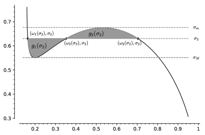
Figure 1. Graph of $\sigma(\omega)$ with $1<\tau<\tau_{*}$. $\sigma_{2}$ is the level where the two shaded regions have the same area or, equivalently, there are two minima.

Remark 3.2.

A proof of the regularity of the one-parameter family defined in (48) exists in dimension $n\geq 3$ as a result of [34, Lemma 20]. The only change needed in the quoted reference in order to obtain a proof tailored to our assumption is $G^{\prime}(u)$ is a function in $L^{2}$ (instead of $L^{\frac{2n}{n+2}}(\mathbb{R}^{n})$ as in the quoted lemma). The authors also assume that the only $H^{1}_{r}(\mathbb{R}^{n};\mathbb{R})$ solution to $\Delta v-G^{\prime\prime}(R_{\omega})v-(m^{2}-\omega^{2})v=0$ is the zero function. In our case ($n=1$) we do not need such assumption as it follows as a special outcome of the dimension one.

Remark 3.3.

In the case (13) the threshold $\sigma_{*}$ provided in (iv) of Proposition 2, is zero. In fact, given $\sigma>0$ one can choose an element $u$ in $S(\sigma/m)$ such that ${E}_{S}(u)<0$. This follows, for instance, from [4, Lemma 5], under the assumption that $G(s)\lesssim-s^{2+\varepsilon}$ with $0<\varepsilon<4/n$ in a neighbourhood of the origin ([4, $F_{2}$]), which is satisfied indeed with $\varepsilon=2$. Therefore, from (26), $E^{*}(u,m)=\sigma m+{E}_{S}(u)<\sigma m$.

In the next theorem, which concludes this section, we will be able to count the number of positive critical points of $E^{*}$ on $M_{\sigma,r}^{*}$ and to establish for each of them whether it is a minimum or not. Let $K_{\sigma}$ be the set defined in (15) and set

$$Cr_{\sigma}:=\{(R,\omega)\mid\exists\eta\text{ s.t. }dE^{*}(R,\omega)=\eta dC^{*}(R,\omega)\}\cap H^{1}_{r,+}(\mathbb{R};\mathbb{R})$$

which is the set of critical points of $E^{*}$ constrained on $M_{\sigma,r}^{*}$.

Theorem 4.

For every $a,b,m$ such that $\tau(a,b,m)>1$, the number of positive critical points and minima of $E^{*}$ on $M_{\sigma,r}^{*}$ behaves as follows:

1. if $\tau\geq\tau_{*}$ then $|K_{\sigma}|=|Cr_{\sigma}|=1$

2. if $1<\tau<\tau_{*}$ then there are two levels $\sigma_{m}(a,b,m)<\sigma_{M}(a,b,m)$ such that

   1. $|K_{\sigma}|=|Cr_{\sigma}|=1$ if $\sigma<\sigma_{m}$ or $\sigma>\sigma_{M}$

   2. $|Cr_{\sigma}|=2$ and $|K_{\sigma}|=1$ if $\sigma\in\{\sigma_{m},\sigma_{M}\}$

   3. $|Cr_{\sigma}|=3$ and $|K_{\sigma}|=1$ if $\sigma_{m}<\sigma<\sigma_{M}$ with $\sigma\neq\sigma_{2}$

   4. $|Cr_{\sigma}|=3$ and $|K_{\sigma}|=2$ if $\sigma=\sigma_{2}$. That is, there are two minima.

The level $\sigma_{2}$ is the level provided in Theorem 3.

Proof.

From Remark 3.3, Corollary 1 and Theorem 2, for every $\sigma>0$ there exist at least one positive minimum.

The case $\tau\geq\tau_{*}$

From Lemma 2, this is the case where $\sigma$ is a strictly decreasing function. Suppose that there are two positive solutions $(\omega_{1},R_{\omega_{1}})$ and $(\omega_{2},R_{\omega_{2}})$ in $M_{\sigma,r}$. Without loss of generality we can assume that $\omega_{1}\leq\omega_{2}$. If $\omega_{1}=\omega_{2}$, then $R_{\omega_{1}}=R_{\omega_{2}}$ by the uniqueness result [6, Proof of Theorem 5]. If $\omega_{1}<\omega_{2}$, then $\sigma(\omega_{1})>\sigma(\omega_{2})$ gives a contradiction. Since there is only one critical point, it is a minimum.

The case $1<\tau<\tau_{*}$

On the intervals $(0,\sigma_{m})$ and $(\sigma_{M},+\infty)$ we use the same argument as the previous case. Then, there is exactly one positive minimum at each level.

If $\sigma=\sigma_{M}$, the value $\sigma$ is achieved at $\omega_{M}$. From (55) and (53) $\sigma(\omega)$ diverges as $\omega\to\omega_{*}$. Then $\sigma_{M}$ is achieved in a second point $\omega_{2}<\omega_{M}$. The existence of a third point would imply the existence of three critical points for $\sigma$ which is ruled out by Lemma 2. Therefore, $|Cr_{\sigma}|=2$ and only one critical point is a minimum, from Theorem 3.

If $\sigma=\sigma_{m}$, the value $\sigma$ is achieved in $\omega_{m}$. Since $\omega_{m}$ is a local minimum, and $\sigma(\omega)$ converges to 0 as $\omega\to m$, the value $\sigma$ is achieved in a second point $\omega_{2}$. The existence of a third point would imply the existence of three critical points for $\sigma$ which is ruled out by Lemma 2. Then, $|Cr_{\sigma}|=2$ and only one critical point is a minimum, from Theorem 3.

Finally, if $\sigma_{m}<\sigma<\sigma_{M}$, there are three points in $(\omega_{*},m)$ such that $\sigma(\omega)=\sigma$. More precisely, these points can be obtained by applying the Intermediate Value Theorem to the function $\sigma$ on the intervals $(\omega_{*},\omega_{m})$, $(\omega_{m},\omega_{M})$ and $(\omega_{M},m)$. Then $|Cr_{\sigma}|=3$; if $\sigma\neq\sigma_{2}$ only one is a minimum, while if $\sigma=\sigma_{2}$, there are two minima, by Theorem 3. ∎ In the formulation of the initial value problem in (48), we restricted to positive solutions. However, if $(R_{\omega},\omega)$ is a critical point, then $(-R_{\omega},\omega)$ is also a critical point. So, $2|Cr_{\sigma}|$ and $2|K_{\sigma}|$ are the number of critical points and minima of $E^{*}$ on $M_{\sigma,r}^{*}$ regardless of the sign.

Remark 3.4.

In [7, Lemma 3.6], C. Bonanno proved that for the non-linear Klein-Gordon equation in dimension $n\geq 3$ there exist at least one local minimum on $M_{\sigma,r}^{*}$ for every connected component of the set $\{G<0\}$, provided $\sigma$ is large enough. The conclusions of (iid) of Theorem 4, can be regarded to as an improvement of this result (even if the dimension is different) at least in the case (13): there are two local minima (in fact two minima) despite the set $\{G<0\}$ being connected.

4. The double power case: non-degeneracy of minima

For each level of charge $\sigma$, we will establish which minima are degenerate or not. A critical point $(R_{\omega},\omega)$ is degenerate if and only if the null space of the Hessian bilinear form restricted to the tangent space

(63) $$T_{(R_{\omega},\omega)}M_{\sigma,r}^{*}=\{(v,\eta)\in H^{1}_{r}(\mathbb{R};\mathbb{R})\times\mathbb{R}\mid\eta\|R_{\omega}\|_{L^{2}}^{2}+2\omega(R_{\omega},v)_{L^{2}}=0\}.$$

is non-trivial. The space above is the kernel of the differential of $C^{*}$ at the point $(R_{\omega},\omega)$. From Theorem 2, the Lagrange multiplier of the critical point $(R_{\omega},\omega)$ is $\omega$. In [13, Appendix] we showed that if $G$ is as in (13) then $E^{*}$ and $C^{*}$ are $C^{2}(H^{1}(\mathbb{R};\mathbb{R});\mathbb{R})$. The Hessian of $E_{r}^{*}$, as a constrained functional is given by

$$H(R_{\omega},\omega):=D^{2}E_{r}^{*}(R_{\omega},\omega)-\omega D^{2}C^{*}_{r}(R_{\omega},\omega).$$

Given two vectors $Y:=(v,\eta)$ and $Z:=(w,\kappa)$ in $T_{(R_{\omega},\omega)}M_{\sigma,r}^{*}$, the Hessians of the two functionals $E_{r}^{*}$ and $C^{*}_{r}$ are

$$\begin{split}D^{2}E_{r}^{*}(R,\omega)[Y,Z]&=\eta\kappa\|R_{\omega}\|_{L^{2}}^{2}+2\omega\kappa(R_{\omega},v)_{L^{2}}+2\omega\eta(R_{\omega},w)_{L^{2}}\\ &+D^{2}_{uu}E_{r}^{*}(R_{\omega},\omega)[v,w]\end{split}$$

$$D^{2}C^{*}_{r}(R_{\omega},\omega)[Y,Z]=2\kappa(R_{\omega},v)_{L^{2}}+2\eta(R_{\omega},w)_{L^{2}}+2\omega(v,w)_{L^{2}}.$$

By inspection,

$$\begin{split}D^{2}_{uu}E_{r}^{*}(R_{\omega},\omega)[v,w]&=\int_{-\infty}^{+\infty}v^{\prime}(x)w^{\prime}(x)dx\\ &+\int_{-\infty}^{+\infty}(G^{\prime\prime}(R_{\omega}(x))+m^{2}+\omega^{2})v(x)w(x)dx.\end{split}$$

Then,

(64) $$\begin{split}H(R_{\omega},\omega)[Y,Z]&=\int_{-\infty}^{+\infty}v^{\prime}(x)w^{\prime}(x)dx\\ &+\int_{-\infty}^{+\infty}(G^{\prime\prime}(R_{\omega}(x))+m^{2}-\omega^{2})v(x)w(x)dx+\eta\kappa\|R_{\omega}\|_{L^{2}}^{2}.\end{split}$$

If $v$ is $H^{2}_{r}$, then

(65) $$H(R_{\omega},\omega)[Y,Z]=(L_{+}(v),w)_{L^{2}}+\eta\kappa\|R_{\omega}\|_{L^{2}}^{2},$$

where

$$L_{+}(v):=-v^{\prime\prime}+G^{\prime\prime}(R_{\omega}(x))v+(m^{2}-\omega^{2})v.$$

For every $Y=(v,\eta)$ in $T_{(R_{\omega},\omega)}M_{\sigma,r}^{*}$, we define

(66) $$\begin{split}\xi(v,\eta):=H(R_{\omega},\omega)[Y,Y]&=\int_{-\infty}^{+\infty}|v^{\prime}(x)|^{2}dx\\ &+\int_{-\infty}^{+\infty}(G^{\prime\prime}(R_{\omega}(x))+m^{2}-\omega^{2})v(x)^{2}dx+\eta^{2}\|R_{\omega}\|_{L^{2}}^{2}.\end{split}$$

Since $(R_{\omega},\omega)$ is a minimum, the Hessian is a positive semidefinite bilinear form. Therefore, it is non-degenerate if and only if $H(R_{\omega},\omega)[Y,Y]=0$ implies that $Y=0$ for every vector $Y$. We will follow a similar approach to the one illustrated in the proof of [37, Proposition 2.9]. We denote with $S(T_{(R_{\omega},\omega)}M_{\sigma,r}^{*})$ the unit sphere with respect to the norm $\|(v,\eta)\|^{2}=\eta^{2}+\|v\|_{L^{2}}^{2}$.

Proposition 5.

The minima $(R_{\omega},\omega)$ and $(-R_{\omega},\omega)$ are non-degenerate if and only if $\sigma^{\prime}(\omega)\neq 0$.

Proof.

Firstly, we show that from $\sigma^{\prime}(\omega)\neq 0$ it follows that $\inf(\xi)>0$ on the unit sphere $S(T_{(R_{\omega},\omega)}M_{\sigma,r}^{*})$. On the contrary, we can suppose that the $\inf(\xi)=0$, because $(R_{\omega},\omega)$ is a minimum. We prove that the infimum is achieved. Let $(\eta_{n},v_{n})$ be a minimizing sequence in $S(T_{(R_{\omega},\omega)}M_{\sigma,r}^{*})$. Since $\eta_{n}^{2}+\|v_{n}\|_{L^{2}}^{2}=1$, the sequence $(\eta_{n})$ is bounded. Up to extract a subsequence, we can suppose that there exist $\eta$ in $\mathbb{R}$ such that

$$\lim_{n\to+\infty}\eta_{n}=\eta.$$

Since $R_{\omega}$ is in $L^{\infty}(\mathbb{R};\mathbb{R})$, the function $G^{\prime\prime}$ can be estimated by a single power, that is, $|G^{\prime\prime}(R_{\omega}(x))|\leq c|R_{\omega}(x)|^{2}$ for some $c$ in $\mathbb{R}$. By applying the Cauchy-Schwarz inequality to $(|R_{\omega}|^{2},v_{n}^{2})_{L^{2}}$, and(33) with $p=4$, we obtain

$$\begin{split}\int_{-\infty}^{+\infty}G^{\prime\prime}(R_{\omega}(x))v_{n}(x)^{2}dx&\geq-s_{GN}^{2}c\|R_{\omega}\|_{L^{4}}^{2}\|v_{n}^{\prime}\|_{L^{2}}^{\frac{1}{2}}\|v_{n}\|_{L^{2}}^{\frac{3}{2}}\\ &\geq-s_{GN}^{2}c\|R_{\omega}\|_{L^{4}}^{2}\|v_{n}^{\prime}\|_{L^{2}}^{\frac{1}{2}}.\end{split}$$

The second inequality follows from $\eta_{n}^{2}+\|v_{n}\|_{L^{2}}^{2}\leq 1$. Since $\frac{1}{2}<2$, the sequence $(v_{n}^{\prime})$ is bounded as well. Then, up to extract a subsequence, we can suppose that there exist $v$ such that $(v_{n})$ converges to $v$ in $L^{\infty}(\mathbb{R};\mathbb{R})$ and weakly in $H^{1}(\mathbb{R};\mathbb{R})$. Then $\lim_{n\to+\infty}G^{\prime\prime}(R_{\omega})v_{n}^{2}=G^{\prime\prime}(R_{\omega})v^{2}$ in $L^{1}(\mathbb{R};\mathbb{R})$. In fact, the sequence $(G^{\prime\prime}(R_{\omega})v_{n}^{2})$ converges pointwise almost everywhere to $G^{\prime\prime}(R_{\omega})v^{2}$ and it is dominated by $c|R_{\omega}|^{2}(\sup_{n}\|v_{n}\|_{\infty}^{2})$ which is $L^{1}$, because it has exponential decay from (3) of Proposition 4. From the weak convergence $v_{n}\rightharpoonup v$ in $L^{2}$ it also follows that $(v,\eta)$ is in $T_{(R_{\omega},\omega)}M_{\sigma,r}^{*}$. Also $v\neq 0$; on the contrary $(G^{\prime\prime}(R_{\omega})v_{n}^{2})$ would converge to zero in $L^{1}$ and, from (66), we would obtain that

$$\begin{split}\xi(v_{n},\eta_{n})&\geq\int_{-\infty}^{+\infty}(G^{\prime\prime}(R_{\omega}(x))+m^{2}-\omega^{2})v_{n}(x)^{2}dx+\eta_{n}^{2}\|R_{\omega}\|_{L^{2}}^{2}\\ &=o(1)+(m^{2}-\omega^{2})(1-\eta_{n}^{2})+\eta_{n}^{2}\|R_{\omega}\|_{L^{2}}^{2}\\ &=o(1)+(m^{2}-\omega^{2})(1-\eta^{2})+\eta^{2}\|R_{\omega}\|_{L^{2}}^{2}\end{split}$$

From Theorem 2, $m^{2}-\omega^{2}>0$. Therefore, taking the limit, we would obtain that $\eta^{2}$ is equal to 0 and 1 at the same time. Then, we can define

(67) $$(v_{*},\eta_{*}):=\left(\frac{v}{\|v\|_{L^{2}}},\frac{\eta}{\|v\|_{L^{2}}}\right)\in S(T_{(R_{\omega},\omega)}M_{\sigma,r}^{*}).$$

Summing up, we have

$$\begin{split}\xi(\eta_{n},v_{n})\geq o(1)+\xi(\eta,v)=o(1)+\|v\|_{L^{2}}^{2}\,\xi(\eta_{*},v_{*}).\end{split}$$

The first inequality is given by the lower-semicontinuity property of the $L^{2}$ norm. The limit in the first term is zero, while the limit in the third term in non-negative. Therefore, $\xi(v_{*},\eta_{*})=0$. Then the infimum of $\xi$ is achieved. Since $(v_{*},\eta_{*})$ is a critical point of $\xi$ constrained to $S(T_{(R_{\omega},\omega)}M_{\sigma,r}^{*})$, there exist $\beta,\gamma>0$ such that

$$\nabla\xi(v_{*},\eta_{*})=\beta\big{(}2\omega R_{\omega},\|R_{\omega}\|_{L^{2}}^{2}\big{)}+\gamma(v_{*},\eta_{*})$$

Since $\nabla\xi(v_{*},\eta_{*})\cdot(v_{*},\eta_{*})=2\xi(v_{*},\eta_{*})=0$, we have $\gamma=0$. This means that $(v_{*},\eta_{*})$ is a solution of the system

$$-2v_{*}^{\prime\prime}+2(G^{\prime\prime}(R_{\omega}(x))+m^{2}-\omega^{2})v_{*}=2\omega\beta R_{\omega},\quad 2\eta_{*}\|R_{\omega}\|_{L^{2}}^{2}=\beta\|R_{\omega}\|_{L^{2}}^{2}$$

which gives

$$v_{*}^{\prime\prime}-(G^{\prime\prime}(R_{\omega}(x))+m^{2}-\omega^{2})v_{*}=-2\omega\eta_{*}R_{\omega}.$$

Taking the derivative with respect to $\omega$ in (48), we obtain

(68) $$(\partial_{\omega}R_{\omega})^{\prime\prime}-(G^{\prime\prime}(R_{\omega}(x))+m^{2}-\omega^{2})\partial_{\omega}R_{\omega}=-2\omega R_{\omega}.$$

Therefore, $w:=v_{*}-\eta_{*}\partial_{\omega}R_{\omega}$, is a solution to the differential equation

(69) $$w^{\prime\prime}-(G^{\prime\prime}(R_{\omega}(x))+m^{2}-\omega^{2})w=0.$$

Since both $v_{*}$ and $\partial_{\omega}R_{\omega}$ are even, $w$ is also even. However, the space of solutions in $H^{1}(\mathbb{R};\mathbb{R})$ of the equation above is generated by $R^{\prime}_{\omega}$, which is an odd function. Therefore, $w\equiv 0$ and $v_{*}=\eta_{*}\partial_{\omega}R_{\omega}$. Since $(v_{*},\eta_{*})$ is orthogonal to $(2\omega R_{\omega},\|R_{\omega}\|_{L^{2}}^{2})$, we have

$$\begin{split}0&=(v_{*},\eta_{*})\cdot(2\omega R_{\omega},\|R_{\omega}\|_{L^{2}}^{2})=(\eta_{*}\partial_{\omega}R_{\omega},\eta_{*})\cdot(2\omega R_{\omega},\|R_{\omega}\|_{L^{2}}^{2})\\ &=\eta_{*}(\partial_{\omega}R_{\omega},1)\cdot(2\omega R_{\omega},\|R_{\omega}\|_{L^{2}}^{2})=\eta_{*}\sigma^{\prime}(\omega).\end{split}$$

We can rule out the case $\eta_{*}=0$ and then obtain a contradiction with the assumption that $\sigma^{\prime}(\omega)\neq 0$. If $\eta_{*}=0$, then $v_{*}$ is an even solution to (69) and thus equal to 0, which contradicts (67). This proves one of the two implications of the lemma.

Conversely, if $(R_{\omega},\omega)$ is non-degenerate, that is the infimum of $\xi$ on $S(T_{(R_{\omega},\omega)}M_{\sigma,r}^{*})$ is positive, then $\sigma^{\prime}(\omega)\neq 0$. On the contrary

$$0=\sigma^{\prime}(\omega)=\|R_{\omega}\|_{L^{2}}^{2}+2\omega(R_{\omega},\partial_{\omega}R_{\omega})_{L^{2}}=(\partial_{\omega}R_{\omega},1)\cdot(2\omega R_{\omega},\|R_{\omega}\|_{L^{2}}^{2}).$$

Therefore, $(\partial_{\omega}R_{\omega},1)$ belongs to $T_{(R_{\omega},\omega)}M_{\sigma,r}^{*}$. Taking the scalar product in $L^{2}(\mathbb{R};\mathbb{R})$ with $-\partial_{\omega}R_{\omega}$ in (68), we obtain

$$\begin{split}0&=\int_{-\infty}^{+\infty}|(\partial_{\omega}R_{\omega})^{\prime}|^{2}dx+\int_{-\infty}^{+\infty}(G^{\prime\prime}(R_{\omega}(x))+m^{2}-\omega^{2})(\partial_{\omega}R_{\omega})^{2}dx\\ &-2\int_{-\infty}^{+\infty}\omega R_{\omega}\partial_{\omega}R_{\omega}dx\\ &=\int_{-\infty}^{+\infty}|(\partial_{\omega}R_{\omega})^{\prime}|^{2}dx+\int_{-\infty}^{+\infty}(G^{\prime\prime}(R_{\omega}(x))+m^{2}-\omega^{2})(\partial_{\omega}R_{\omega})^{2}dx+\|R_{\omega}\|_{L^{2}}^{2}\\ &=\xi(\partial_{\omega}R_{\omega},1).\end{split}$$

The second equality follows from $\sigma^{\prime}(\omega)=0$. Therefore, if we set

$$T:=\frac{(\partial_{\omega}R_{\omega},1)}{\sqrt{1+\|\partial_{\omega}R_{\omega}\|_{L^{2}}^{2}}}$$

we have $\xi(T)=0$ contradicting the non-degeneracy assumption. ∎

Theorem 5.

For every $a,b,m$ such that $\tau(a,b,m)>1$,

1. if $\tau\neq\tau_{*}$, then minima are non-degenerate

2. if $\tau=\tau_{*}$ and $\sigma\neq\sigma_{s}$, then minima are non-degenerate. If $\sigma=\sigma_{s}$, then $(R_{\omega_{s}},\omega_{s})$ and $(-R_{\omega_{s}},\omega_{s})$ are degenerate.

Proof.

(i). If $\tau>\tau_{*}$, $\sigma^{\prime}$ is always negative. Therefore, minima are non-degenerate from Theorem 5. If $1<\tau<\tau_{*}$, the derivative of $\sigma$ vanishes at $\omega_{M}$ and $\omega_{m}$; $\sigma_{M}$ is achieved at $\omega_{M}$ and another point $\omega_{1}<\omega_{M}$. We repeat the computation in (62) with $\omega_{M}$ replacing $\omega_{3}$ and $\sigma_{M}$ in place of $\sigma$. Therefore,

$$e(\omega_{M})-e(\omega_{1})=\int_{\omega_{1}}^{\omega_{M}}(\sigma_{M}-\sigma(t))dt>0$$

showing that $E^{*}(R_{\omega_{M}},\omega_{M})>I(\sigma_{M})$ and proving that minima on $M_{\sigma_{M},r}^{*}$ are non-degenerate. Similarly, $\sigma_{m}$ is achieved at $\omega_{m}$ and another point $\omega_{m}<\omega_{3}$. We repeat the computation in (62) with $\omega_{m}$ replacing $\omega_{1}$ and $\sigma_{m}$ in place of $\sigma_{2}$. Therefore,

$$e(\omega_{m})-e(\omega_{1})=\int_{\omega_{1}}^{\omega_{m}}(\sigma_{m}-\sigma(t))dt>0$$

proving that $E_{r}^{*}(R_{\omega_{m}},\omega_{m})>I(\sigma_{m})$. Therefore, minima on $M_{\sigma_{m},r}^{*}$ are non-degenerate.

(ii). From Lemma 2, $\sigma^{\prime}(\omega)\neq 0$ unless $\omega=\omega_{s}$; from Theorem 3, on $M_{\sigma_{s},r}^{*}$ the only critical points are minima. Therefore, both $(R_{\omega_{s}},\omega_{s})$ and $(-R_{\omega_{s}},\omega_{s})$ are degenerate minima. ∎

5. The double power case: stability of standing-waves

In this conclusive section, we prove the orbital stability of standing-wave solutions to (1) when $G$ is the double power $\eqref{eq.DP}$.

Theorem 6.

For the non-linear term (13), the set $\Gamma(\Phi)$ is stable for every $\sigma>0$ and $\Phi$ in $\Gamma_{\sigma}$.

Proof.

We start by looking at the cases (i), (iia), (iib), (iic) of Theorem 4, where there are exactly two minima, $(R_{\omega},\omega)$ and $(-R_{\omega},\omega)$. We claim that

$$\Gamma_{\sigma}=\Gamma(R_{\omega},-i\omega R_{\omega}).$$

The set on the right is a subset of the ground-state by the invariance properties described in (12). From Theorem 2, given $\Phi$ in $\Gamma_{\sigma}$, there exist a pair $(R_{1},\omega_{1})$ and $(y,z)$ in $\mathbb{R}\times S^{1}$ such that

$$\Phi=(zR_{1}(\cdot+y),-i\omega_{1}zR_{1}(\cdot+y)),\quad E_{r}^{*}(R_{1},\omega_{1})=I(\sigma).$$

By Theorem 4, $R_{1}=R_{\omega}$ implying that $\Phi$ is an element of $\Gamma_{\sigma}(R_{\omega},-i\omega R_{\omega})$. Therefore, since $\Gamma_{\sigma}$ is stable by Theorem 1, the set $\Gamma(\Phi)$ is also stable. In the case (iid) of Theorem 4 there are two positive minima $(\omega_{1},R_{\omega_{1}})$ and $(\omega_{2},R_{\omega_{2}})$ in $M_{\sigma_{2},r}^{*}$. Firstly, we show that

(70) $$\delta:=\mathrm{dist}\big{(}\Gamma(R_{\omega_{1}},-i\omega_{1}R_{\omega_{1}}),\Gamma(R_{\omega_{2}},-i\omega_{2}R_{\omega_{2}})\big{)}>0.$$

We consider two arbitrary points $\Phi_{1}$ and $\Phi_{2}$ of the two sets. Therefore, there are $(y_{1},z_{1})$ and $(y_{2},z_{2})$ in $\mathbb{R}\times S^{1}$ such that

$$\Phi_{1}=(z_{1}R_{\omega_{1}}(\cdot+y_{1}),-iz_{1}\omega_{1}R_{\omega_{1}}(\cdot+y_{1})),\ \Phi_{2}=(z_{2}R_{\omega_{2}}(\cdot+y_{2}),-iz_{2}\omega_{2}R_{\omega_{2}}(\cdot+y_{2}))$$

according to the definition given in (11). We have

$$\begin{split}\mathrm{dist}(\Phi_{1},\Phi_{2})^{2}&=\|z_{1}R_{\omega_{1}}(\cdot+y_{1})-z_{2}R_{\omega_{2}}(\cdot+y_{2})\|_{H^{1}}^{2}\\ &+\|iz_{1}\omega_{1}R_{\omega_{1}}(\cdot+y_{1})-iz_{2}\omega_{2}R_{\omega_{2}}(\cdot+y_{2})\|_{L^{2}}^{2}.\end{split}$$

From (2) of Proposition 4, $R_{\omega_{1}}$ and $R_{\omega_{2}}$ are positive and radially decreasing. Therefore

$$\begin{split}&\|z_{1}R_{\omega_{1}}(\cdot+y_{1})-z_{2}R_{\omega_{2}}(\cdot+y_{2})\|_{H^{1}}^{2}\geq\|z_{1}R_{\omega_{1}}(\cdot+y_{1})-z_{2}R_{\omega_{2}}(\cdot+y_{2})\|_{L^{2}}^{2}\\ =&\|R_{\omega_{1}}-z_{2}\overline{z}_{1}R_{\omega_{2}}(\cdot+y_{2}-y_{1})\|_{L^{2}}^{2}\geq\|R_{\omega_{1}}-R_{\omega_{2}}\|_{L^{2}}^{2}.\end{split}$$

The equality follows from a variable change. Therefore,

$$\mathrm{dist}(\Phi_{1},\Phi_{2})\geq\|R_{\omega_{1}}-R_{\omega_{2}}\|_{L^{2}}$$

which provides a lower bound for $\delta$. Hereafter, we will use the notation

(71) $$S_{1}:=\Gamma(R_{\omega_{1}},-i\omega_{1}R_{\omega_{1}}),\quad S_{2}:=\Gamma(R_{\omega_{2}},-i\omega_{2}R_{\omega_{2}}).$$

Since $\delta=\mathrm{dist}(S_{1},S_{2})>0$, in the metric space $\mathbf{X}$ each of the sets $S_{i}$ are isolated from each other. In fact,

(72) $$B(S_{i},\delta)\cap\Gamma_{\sigma_{2}}=S_{i}.$$

For $1\leq i\leq 2$. We define ${E}_{i}:=\inf\{{E}(\Phi)\mid\Phi\in\partial B(S_{i},\delta/2)\cap M_{\sigma_{2}}\}$. We claim that

(73) $${E}_{i}>I(\sigma_{2}).$$

Otherwise, we would have a sequence $(\Phi_{n})$ such that

(74) $${E}(\Phi_{n})\to I(\sigma),\quad C(\Phi_{n})=\sigma_{2}.$$

By Lemma 1, up to extract a subsequence, we can suppose that there exist $\Phi$ in $\Gamma_{\sigma_{2}}$ and $(y_{n})\subseteq\mathbb{R}$ such that

$$\Phi_{n}(\cdot+y_{n})\to\Phi\text{ in }H^{1}(\mathbb{R};\mathbb{C})\times L^{2}(\mathbb{R};\mathbb{C}).$$

Therefore, $\Phi$ is in $\partial B(S_{i},\delta/2)\cap\Gamma_{\sigma_{2}}$, because $\mathrm{dist}(\Phi_{n}(\cdot+y_{n}),S_{i})=\mathrm{dist}(\Phi_{n},S_{i})$. Then, we obtained a contradiction with (72). We are now able to prove that each of these sets is stable. Suppose that $S_{i}$ is not stable for some $i$ in $\{1,2\}$; the other set is $S_{3-i}$. Then, there are sequences $(\Phi_{n})$, $(t_{n})$ and $\varepsilon_{0}>0$ such that

(75) $$\mathrm{dist}(\Phi_{n},S_{i})\to 0,\quad\mathrm{dist}(U(t_{n},\Phi_{n}),S_{i})\geq\varepsilon_{0}.$$

We set $\Psi_{n}:=U(t_{n},\Phi_{n})$. From Theorem 1, the set $\Gamma_{\sigma_{2}}$ is stable, which implies $\mathrm{dist}(\Psi_{n},\Gamma_{\sigma_{2}})\to 0$. From (70), (71) and (75), $\mathrm{dist}(\Psi_{n},S_{3-i})\to 0$. Then, there exist $n_{0}$ such that for every $n\geq n_{0}$ $\mathrm{dist}(\Psi_{n},S_{3-i})<\frac{\delta}{2}$. Then, by (72) $\mathrm{dist}(\Psi_{n},S_{i})\geq\delta/2$. From (7), the following curves

$$\alpha_{n}\colon(-\infty,+\infty)\to\mathbf{X},\quad\alpha_{n}(t)=\left(\frac{\sigma_{2}}{C(\Phi_{n})}\right)^{\frac{1}{2}}U(t,\Phi_{n})$$

all belong to $M_{\sigma_{2}}$. From (74), we can also suppose that ${E}(\alpha_{n}(0))<E_{i}$ for every $n\geq n_{0}$. Therefore,

(76) $${E}(\alpha_{n_{0}}(0))<{E}_{i}$$

(77) $$\mathrm{dist}(\alpha_{n_{0}}(0),S_{i})<\frac{\delta}{2},\quad\mathrm{dist}(\alpha_{n_{0}}(t_{n_{0}}),S_{i})\geq\frac{\delta}{2}.$$

From (77), there exist $\overline{t}$ such that $\mathrm{dist}(\alpha_{n_{0}}(\overline{t}),S_{i})=\delta/2$. Then $\alpha_{n_{0}}(\overline{t})$ is in $\partial B(S_{i},\delta/2)\cap M_{\sigma_{2}}$. From (7), ${E}(\alpha_{n_{0}}(0))={E}(\alpha_{n_{0}}(\overline{t}))$. Therefore, ${E}(\alpha_{n_{0}}(\overline{t}))<{E}_{i}$, which contradicts (73). ∎

The case $\sigma=0$

We conclude this section by looking at the case $\sigma=0$, which we include for the sake of completeness. If $\sigma=0$, from (G1) the minimum of ${E}$ is achieved only by the pair $(0,0)\in\mathbf{X}$. Therefore, $\Gamma_{0}=\{(0,0)\}$. The stability of $\Gamma_{0}$ relies only on the continuity and the coercivity of ${E}$.

Proposition 6.

$\Gamma_{0}$ is stable.

Proof.

Given $\varepsilon>0$, by (iii) of Proposition 1 there exist $e>0$ such that $h_{1}(e)<\varepsilon$. By (v) of the same proposition, there exist $\delta>0$ such that $\|\Phi\|_{\mathbf{X}}<\delta$ implies ${E}(\Phi)<e$. We also notice that $\mathrm{dist}(\Phi,\Gamma_{0})=\|\Phi\|_{\mathbf{X}}$. Then, given $\Phi$ such that $\mathrm{dist}(\Phi,\Gamma_{0})<\delta$, we also have $\|\Phi\|_{\mathbf{X}}<\delta$. Then ${E}(\Phi)<e$ by the continuity of ${E}$. From (7), ${E}(U(t,\Phi))<e$ for every $t$. Then $\|U(t,\Phi)\|_{\mathbf{X}}<h_{2}(e)<\varepsilon$ by (iii) of Proposition 1. Therefore $\mathrm{dist}(U(t,\Phi))<\varepsilon$ for every $t$, which concludes the proof. ∎

References

- [1] Antonio Ambrosetti and Giovanni Prodi. A primer of nonlinear analysis, volume 34 of Cambridge Studies in Advanced Mathematics. Cambridge University Press, Cambridge, 1993.
- [2] Thomas Bartsch and Nicola Soave. Multiple normalized solutions for a competing system of Schrödinger equations. Calc. Var. Partial Differential Equations, 58(1):Art. 22, 24, 2019.
- [3] J. Bellazzini, V. Benci, C. Bonanno, and A. M. Micheletti. Solitons for the nonlinear Klein-Gordon equation. Adv. Nonlinear Stud., 10(2):481–499, 2010.
- [4] J. Bellazzini, V. Benci, M. Ghimenti, and A. M. Micheletti. On the existence of the fundamental eigenvalue of an elliptic problem in . Adv. Nonlinear Stud., 7(3):439–458, 2007.
- [5] Vieri Benci and Donato Fortunato. Hylomorphic solitons and charged Q-balls: Existence and stability. Chaos Solitons Fractals, 58:1–15, 2014.
- [6] H. Berestycki and P.-L. Lions. Nonlinear scalar field equations. I. Existence of a ground state. Arch. Rational Mech. Anal., 82(4):313–345, 1983.
- [7] Claudio Bonanno. Existence and multiplicity of stable bound states for the nonlinear Klein-Gordon equation. Nonlinear Anal., 72(3-4):2031–2046, 2010.
- [8] Jean Bourgain, Haim Brezis, and Petru Mironescu. Lifting in Sobolev spaces. J. Anal. Math., 80:37–86, 2000.
- [9] Haïm Brézis and Elliott Lieb. A relation between pointwise convergence of functions and convergence of functionals. Proc. Amer. Math. Soc., 88(3):486–490, 1983.
- [10] Jaeyoung Byeon, Louis Jeanjean, and Mihai Mariş. Symmetry and monotonicity of least energy solutions. Calc. Var. Partial Differential Equations, 36(4):481–492, 2009.
- [11] T. Cazenave and P.-L. Lions. Orbital stability of standing waves for some nonlinear Schrödinger equations. Comm. Math. Phys., 85(4):549–561, 1982.
- [12] Simão Correia. Stability of ground-states for a system of coupled semilinear Schrödinger equations. NoDEA Nonlinear Differential Equations Appl., 23(3):Art. 26, 14, 2016.
- [13] D. Garrisi and V. Georgiev. Orbital stability and uniqueness of the ground state for the non-linear Schrödinger equation in dimension one. Discrete Contin. Dyn. Syst., 37(8):4309–4328, 2017.
- [14] Daniele Garrisi. On the orbital stability of standing-wave solutions to a coupled non-linear Klein-Gordon equation. Adv. Nonlinear Stud., 12(3):639–658, 2012.
- [15] J. Ginibre and G. Velo. The global Cauchy problem for the nonlinear Klein-Gordon equation. Math. Z., 189(4):487–505, 1985.
- [16] Tianxiang Gou and Louis Jeanjean. Existence and orbital stability of standing waves for nonlinear schrödinger systems. Nonlinear Analysis, 144:10–22, 2016.
- [17] Manoussos Grillakis, Jalal Shatah, and Walter Strauss. Stability theory of solitary waves in the presence of symmetry. I. J. Funct. Anal., 74(1):160–197, 1987.
- [18] Manoussos Grillakis, Jalal Shatah, and Walter Strauss. Stability theory of solitary waves in the presence of symmetry. II. J. Funct. Anal., 94(2):308–348, 1990.
- [19] Norihisa Ikoma. Compactness of minimizing sequences in nonlinear Schrödinger systems under multiconstraint conditions. Adv. Nonlinear Stud., 14(1):115–136, 2014.
- [20] Man Kam Kwong. Uniqueness of positive solutions of in . Arch. Rational Mech. Anal., 105(3):243–266, 1989.
- [21] T. D. Lee. Particle physics and introduction to field theory, volume 1 of Contemporary Concepts in Physics. Harwood Academic Publishers, Chur, 1981. Translated from the Chinese.
- [22] Elliott H. Lieb and Michael Loss. Analysis, volume 14 of Graduate Studies in Mathematics. American Mathematical Society, Providence, RI, second edition, 2001.
- [23] P.-L. Lions. The concentration-compactness principle in the calculus of variations. The locally compact case. I. Ann. Inst. H. Poincaré Anal. Non Linéaire, 1(2):109–145, 1984.
- [24] P.-L. Lions. The concentration-compactness principle in the calculus of variations. The locally compact case. II. Ann. Inst. H. Poincaré Anal. Non Linéaire, 1(4):223–283, 1984.
- [25] Chuangye Liu, Nghiem V. Nguyen, and Zhi-Qiang Wang. Existence and stability of solitary waves of an -coupled nonlinear Schrödinger system. J. Math. Study, 49(2):132–148, 2016.
- [26] Kevin McLeod. Uniqueness of positive radial solutions of in . II. Trans. Amer. Math. Soc., 339(2):495–505, 1993.
- [27] Kevin McLeod and James Serrin. Uniqueness of positive radial solutions of in . Arch. Rational Mech. Anal., 99(2):115–145, 1987.
- [28] Nghiem V. Nguyen and Zhi-Qiang Wang. Orbital stability of solitary waves for a nonlinear Schrödinger system. Adv. Differential Equations, 16(9-10):977–1000, 2011.
- [29] Benedetta Noris, Hugo Tavares, and Gianmaria Verzini. Existence and orbital stability of the ground states with prescribed mass for the -critical and supercritical NLS on bounded domains. Anal. PDE, 7(8):1807–1838, 2014.
- [30] Benedetta Noris, Hugo Tavares, and Gianmaria Verzini. Stable solitary waves with prescribed -mass for the cubic Schrödinger system with trapping potentials. Discrete Contin. Dyn. Syst., 35(12):6085–6112, 2015.
- [31] Benedetta Noris, Hugo Tavares, and Gianmaria Verzini. Normalized solutions for nonlinear Schrödinger systems on bounded domains. Nonlinearity, 32(3):1044–1072, 2019.
- [32] Masahito Ohta. Stability of solitary waves for coupled nonlinear Schrödinger equations. Nonlinear Anal., 26(5):933–939, 1996.
- [33] Jalal Shatah. Stable standing waves of nonlinear Klein-Gordon equations. Comm. Math. Phys., 91(3):313–327, 1983.
- [34] Jalal Shatah and Walter Strauss. Instability of nonlinear bound states. Comm. Math. Phys., 100(2):173–190, 1985.
- [35] Masataka Shibata. Stable standing waves of nonlinear Schrödinger equations with a general nonlinear term. Manuscripta Math., 143(1-2):221–237, 2014.
- [36] Terence Tao. Nonlinear dispersive equations, volume 106 of CBMS Regional Conference Series in Mathematics. Published for the Conference Board of the Mathematical Sciences, Washington, DC, 2006. Local and global analysis.
- [37] Michael I. Weinstein. Modulational stability of ground states of nonlinear Schrödinger equations. SIAM J. Math. Anal., 16(3):472–491, 1985.