A BCG WITH OFFSET COOLING: IS THE AGN FEEDBACK CYCLE BROKEN IN A2495?

Abstract

We present a combined radio/X-ray analysis of the poorly studied galaxy cluster Abell 2495 (z=0.07923) based on new EVLA and Chandra data. We also analyze and discuss H$\alpha$ emission and optical continuum data retrieved from the literature. We find an offset of $\sim$ 6 kpc between the cluster BCG (MCG+02-58-021) and the peak of the X-ray emission, suggesting that the cooling process is not taking place on the central galaxy nucleus. We propose that sloshing of the ICM could be responsible for this separation. Furthermore, we detect a second, $\sim$ 4 kpc offset between the peak of the H$\alpha$ emission and that of the X-ray emission. Optical images highlight the presence of a dust filament extending up to $\sim$ 6 kpc in the cluster BCG, and allow us to estimate a dust mass within the central 7 kpc of 1.7 $\cdot$ 10⁵ M_☉. Exploiting the dust to gas ratio and the $L_{\text{H}\alpha}$-$M_{\text{mol}}$ relation, we argue that a significant amount (up to 10⁹ M_☉) of molecular gas should be present in the BCG of this cluster. We also investigate the presence of ICM depressions, finding two putative systems of cavities; the inner pair is characterized by $t_{\text{age}}\sim 18$ Myr and $P_{\text{cav}}\sim$ 1.2 $\cdot$ 10⁴³ erg s^-1, the outer one by $t_{\text{age}}\sim 53$ Myr and $P_{\text{cav}}\sim$ 5.6 $\cdot$ 10⁴² erg s^-1. Their age difference appears to be consistent with the free-fall time of the central cooling gas and with the offset timescale estimated with the H$\alpha$ kinematic data, suggesting that sloshing is likely playing a key role in this environment. Furthermore, the cavities’ power analysis shows that the AGN energy injection is able to sustain the feedback cycle, despite cooling being offset from the BCG nucleus.

1 Introduction

The classical cooling flow model predicted that the intra-cluster medium (ICM) of cool-core galaxy clusters should cool, condense and accrete onto the brightest cluster galaxy (BCG), forming stars and producing strong line emission radiation (Fabian et al., 1994). These features are seen in many galaxy clusters, but both at a rate $\sim 1-10$ $\%$ of that expected in the standard model (Peterson & Fabian, 2006).
It is now widely recognized that cooling of the central gas is quenched by Active Galactic Nuclei (AGN) found in the BCGs of clusters (McNamara & Nulsen, 2007; Gitti et al., 2012; Fabian, 2012). In this ”radio-mode” mechanical feedback, radio jets or outflows inflate bubbles (seen as X-ray brightness depressions named cavities) and generate shock waves and cold fronts in the hot atmosphere of the cluster (McNamara et al., 2000; Fabian et al., 2006). The AGN is fueled through Super Massive Black Hole (SMBH) accretion of the same gas condensing from the central regions (Gaspari et al., 2011, 2013; Soker & Pizzolato, 2005), establishing a feedback loop in which the various components are able to regulate each other. This hypothesis is supported by the correlation between the AGN mechanical power, estimated from the X-ray cavities, and the ICM cooling rate (e.g., Bîrzan et al., 2004; Rafferty et al., 2006).
BCGs at the center of galaxy clusters often host a rich multiphase medium which can extend for tens of kpc, as revealed by strong line emission from ionized (warm) and molecular (cold) gas (Crawford et al., 1999; Hamer et al., 2016; McDonald et al., 2010, 2014; Russell et al., 2019, and references therein). The warm and cold gas show correlations with each other and with the hot ICM (Crawford et al., 1999; Edge, 2001; Hogan et al., 2017; Pulido et al., 2018), which strongly suggest that hot gas cooling (albeit reduced with respect to the classical cooling flow model) is the origin of the observed cold gas. Observations, simulations and analytic investigations agree that spatially extended cooling is likely to occur in dense cool cores with short cooling times (or cooling time/dynamical time ratio below certain threshold, e.g., Hogan et al., 2017; Pulido et al., 2018, and references therein). The multiphase medium in cluster cores also reveals a complex dynamics, likely the result of AGN activity and merging events. Chaotic (turbulent) motion and outflows are common (Heckman et al., 1989; Hamer et al., 2016; Russell et al., 2019). It seems reasonable that cold gas inherits the disturbed dynamics from the (low entropy) hot gas from which it has cooled (McDonald et al., 2010; McNamara et al., 2016; Gaspari et al., 2018).
In dynamically-relaxed systems, we expect the BCG to be at the centre of the cluster potential well, as described by the ’central galaxy paradigm’ (van den Bosch et al., 2005; Cui et al., 2016). In this scenario, the galaxy should be coincident both with the cluster cool core centre (i.e. the X-ray peak) and with the line emission peak. However, in the case of interactions with other clusters or halos, all these components are likely to shift, leading to the production of offsets between them. The connection between offsets and the dynamical state of clusters has been investigated both by observational studies (Katayama et al., 2003; Patel et al., 2006; Rossetti et al., 2016), making use of the current generation of X-ray satellites (e.g., Chandra and XMM-Newton), and simulations (Skibba et al., 2011). Hudson et al. (2010) studied a sample of 64 cool-core (CC) and non cool-core (NCC) clusters, finding that objects with a projected distance $>50$ h${}^{-1}_{71}$ kpc between the BCG and the X-ray peak (12% of the sample) typically show large-scale radio emission, that is believed to be associated with major mergers; these clusters are usually NCC. On the other hand, the vast majority (80%) of CC present an offset $<50$ h${}^{-1}_{71}$ kpc; among these, only 2 clusters show large-scale radio emission. A similar study by Sanderson et al. (2009) on a sample of 65 CC clusters found that stronger cool cores are associated with smaller offsets, since more dynamically-disturbed objects have likely undergone a stronger merging phase that produced a disruptive impact on the X-ray core. The same trend was confirmed by Mittal et al. (2009). Offsets of the line emission peak are significant for the comprehension of the clusters dynamical evolution, too: detecting 10⁴ K gas shifted from the BCG (e.g., Sharma_2004) could suggest that cooling of the ICM is able to reach low temperatures even outside the central galaxy environment (Hamer et al., 2012).
These works have established the correlation between offsets and clusters dynamical state (e.g., Rossetti et al., 2016), which can therefore be used in order to discriminate between dynamically relaxed and non-relaxed objects (e.g., Sanderson et al., 2009; Hudson et al., 2010; Mann & Ebeling, 2012).

This work is a multi-frequency study of Abell 2495 (A2495). This object was selected from the ROSAT BCS Sample (Ebeling et al., 1998) by choosing objects with X-ray fluxes greater than $10^{-11}$ erg cm^-2 s^-1 (1.18 $\cdot 10^{-11}$ erg cm^-2 s^-1 for A2495) and, among these, by selecting those characterized by L${}_{H\alpha}>$ 10⁴⁰ erg s^-1 from the catalogue of Crawford et al. (1999). Following these criteria, we obtained a compilation of 13 objects, including some of the best-studied galaxy clusters (e.g., A1795, A478); among all these objects, A2495 and A1668 were still unobserved by Chandra. We thus proposed joint Chandra/VLA observations (P.I. Gitti) of these two clusters and were awarded time in Chandra cycles 11 and 12. This paper presents our results for A2495, and a forthcoming paper will describe A1668 (Pasini et al., in preparation). A2495 was previously observed by NVSS, which provides an estimate of the 1.4 GHz flux of F(1.4 GHz) = 14.7 $\pm$ 0.6 mJy, and by TGSS, from which F(150 MHz) $\simeq$ 136 mJy. We also discuss H$\alpha$ data from Hamer et al. (2016) and exploit optical images (P.I. Zaritsky) from the Hubble Space Telescope (HST) archive. With this broad data coverage we are in the position to perform a multi-wavelength investigation of this cluster, that will allow us to better understand the dynamical interactions between the hot ICM, the colder gas and the radio galaxy hosted in the BCG.
We adopt a $\Lambda$CDM cosmology with $H_{0}$ = 73 km s^-1 Mpc^-1, $\Omega_{M}$= $1-\Omega_{\Lambda}$ = 0.3, and assumed the BCG redshift $z$ = 0.07923 (Rines et al., 2016; Hamer et al., 2016) for the cluster as a whole. The luminosity distance is 345 Mpc, leading to a conversion of 1^′′ = 1.44 kpc.

2 Radio analysis

2.1 Observations and data reduction

We performed new observations of the radio source associated with A2495 BCG ($RA$ = 22${}^{\text{h}}$50${}^{\text{m}}$19.7${}^{\text{s}}$, $DEC$ = +10$\degree$54${}^{\text{m}}$12.7${}^{\text{s}}$, J2000) at 5 GHz and 1.4 GHz with the EVLA in, respectively, B and A configuration (for details, see Table 1).

Data	P.I.	Project Code	Number of spw	Channels	Bandwith	Array	Total exposure time
5 GHz (C BAND)	M. Gitti	SC0143	2 (4832 MHz - 4960 MHz)	64	128 MHz	B	7h58m35s
1.4 GHz (L BAND)	M. Gitti	SC0143	2 (1264 MHz - 1392 MHz)	64	128 MHz	A	3h59m22s

Table 1: Radio observations properties.

For both the observations the source 3C48 (J0137+3309) was used as primary flux calibrator; for the 5 GHz observation, that was split into two datasets, J2241+0953 was used as secondary phase calibrator and 3C48 as polarization calibrator; for the 1.4 GHz observation, J2330+1100 was used as both secondary phase and polarization calibrator.
The data reduction was performed with the NRAO Common Astronomy Software Applications package (CASA), version 5.3. We applied the standard calibration procedure on each dataset and carried out an accurate editing of the visibilities. We performed both manual and automatic flagging (task FLAGDATA, mode= manual and rflag) to exclude radio frequency interferences (RFI) and corrupted data. As a result, we removed about 10% of the visibilities in the 5 GHz band and about 20% in the 1.4 GHz band. We also attempted the self-calibration on the target, but the operation was not successful probably due to the source faintness.
We then applied the standard imaging procedure, using the CLEAN task, on a 7^′′ $\times$ 7^′′ region centered on the cluster. We made use of the gridmode=WIDEFIELD option in order to parametrize the sky curvature; we also set a two-terms approximation of the spectral model by using nterms=2 (MS-MFS algorithm, Rau & Cornwell (2011)) and performed a multi-scale clean (multiscale=[0,5,24]), in order to better reconstruct the faint extended emission.

2.2 Results

For each observing band, we produced maps by setting weighting=BRIGGS and ROBUST 0, in order to obtain the best combination of resolution and sensitivity. The NATURAL and UNIFORM maps, that respectively enhance the sensitivity and the resolution, did not exhibit any interesting feature compared to the ROBUST 0 image, so they are not shown here. Typical amplitude calibration errors of our data were at 8$\%$: this is the uncertainty we assumed for the flux density measurements.

2.2.1 5 GHz map

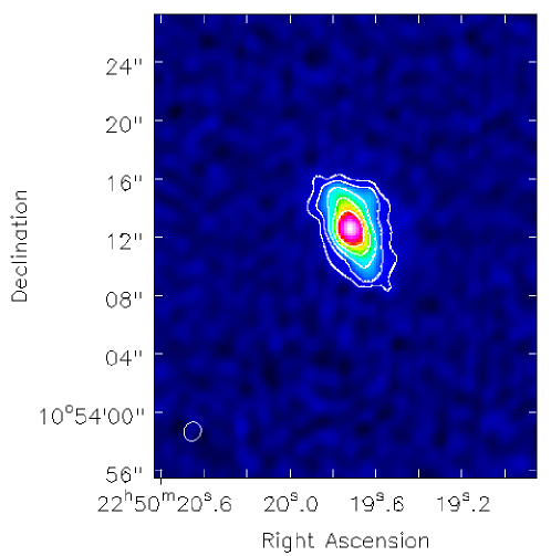
Figure 1: 5 GHz map (ROBUST 0) of A2495. The resolution is 1.30^′′ $\times$ 1.15^′′, with a RMS noise of 4 $\mu$Jy beam^-1. Countours are at -3,3,6,12,24,48 $\cdot$ RMS. The source flux is 2.37 $\pm$ 0.19 mJy. The bottom-left circle represents the beam.

The 5 GHz map (Fig. 1) is characterized by a resolution of 1.30^′′ $\times$ 1.15^′′ and a RMS noise of $4\ \mu$Jy  beam^-1. The total 5 GHz flux of the radio source in A2495 is 2.37 $\pm$ 0.19 mJy. This result is slightly different from Hogan et al. (2015), who measured a source flux of 2.85 $\pm$ 0.09 mJy in C array. This difference can be produced either by observational or intrinsic effects: the maximum baseline of C configuration, used by Hogan et al. (2015), is shorter with respect to the B array, therefore its brightness sensitivity is higher; on the other hand, short-timescale (weeks to months) 10-30% flux variations in radiogalaxies have recently been observed, especially in cool core cluster’s BCGs (e.g., Dutson_2014; Hogan_2015b).
We find that the radio emission is produced by the central radio galaxy on a scale of $\sim$ 10^′′; we do not observe any feature of diffuse emission. Following the method described by Feretti & Giovannini (2008), we estimated the equipartition field, finding $B_{eq}$(5 GHz) = 3.81 $\pm$ 0.05 $\mu$G, consistent with the typical values characterizing radio galaxies.
We used stokes=Q and stokes=U maps in order to get informations about the radio source polarization, and found that the polarization percentage at 5 GHz is about 5$\%$. Table 2 summarizes the radio properties of the source on each band.

Band	Flux	Luminosity(a)	Volume	Brightness Temperature	Equipartition Field	Polarisation
	[mJy]	[1022 W Hz-1]	[kpc3]	[K]	[$\mu$G]
5 GHz	2.37 $\pm$ 0.19	3.3 $\pm$ 0.3	616 $\pm$ 56	3.7 $\pm$ 0.9	3.81 $\pm$ 0.05	5$\%$
1.4 GHz	15.70 $\pm$ 1.30	21.8 $\pm$ 1.8	1112 $\pm$ 78	232 $\pm$ 49	5.60 $\pm$ 0.07	$\leq$ 1$\%$

Table 2: Radio properties of A2495. The volume is estimated assuming a prolate elissoid shape, where the axes are a = 13.6 $\pm$ 1.8 kpc, b = 9.3 $\pm$ 1.8 kpc for the 5 GHz map and a = 13.6 $\pm$ 1.8 kpc, b = 12.5 $\pm$ 1.8 kpc for the 1.4 GHz map.
${(a)}$: estimated using L_ν = $4\pi\cdot(D_{L})^{2}\cdot F_{\nu}\cdot(1+z)^{\alpha-1}$, where $D_{L}$ is the luminosity distance, $F_{\nu}$ is the flux at the frequency $\nu$ and $\alpha$ is the mean spectral index (see Sec. 2.2.3).

2.2.2 1.4 GHz map

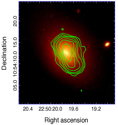
Figure 2: 1.4 GHz contours (ROBUST 0) of the radio source overlaid on an HST image (F606W filter) of A2495. The resolution of the radio map is 1.29^′′ $\times$ 1.12^′′, with a RMS noise of 10 $\mu$Jy beam^-1. Countours are at -3,3,6,12,24,48 $\cdot$ RMS. The source flux is 15.7$\pm$ 1.3 mJy.

In Fig. 2 we overlaid the 1.4 GHz contours on an optical image (F606W filter) retrieved from the HST Archive. The total source flux at this frequency is 15.7 $\pm$ 1.3 mJy, in agreement with the estimation made by Owen & Ledlow (1997) of $\sim$ 14 mJy. The radio source emission entirely lies on the BCG, whose major axis measures $\sim$ 25 kpc; there are no apparent hints of emission on larger scales. This is confirmed by the lack of additional flux on short baselines and by the flux estimate given by NVSS (see Section 1), consistent with ours. The radio galaxy morphology is very similar to the one at 5 GHz, extending on a scale of about $\sim$ 10^′′ ($\sim$ 14 kpc). Radio properties at 1.4 GHz can be found in Table 2.
The 1.4 GHz luminosity is 2.18 $\cdot$ 10²³ W Hz^-1: the radio source in A2495 can be classified as FRI galaxy, characterised by asymmetric lobes and absence of hotspots. Similarly to what done at 5 GHz, we estimated the equipartition field, finding 5.60 $\pm$ 0.07 $\mu$G, and determined an upper limit of $\sim$ 1$\%$ for the polarization.
Hogan et al. (2015) performed a study of the radio properties of a large sample of BCGs, producing the luminosity function at 1.4 GHz of the BCS Sample. Notably, our luminosity estimate places A2495 in the 80${}^{\text{th}}$ percentile of the function (see Fig.4 of Hogan et al. 2015); of the 13 clusters that meet our selection criteria, it is the least radio powerful.

2.2.3 Spectral index map

We produced the spectral index map, via the CASA task IMMATH, by combining the 1.4 GHz and the 5 GHz ones produced by setting weighting=UNIFORM, uvrange=6-178 (in order to match uvranges between the two bands), with a resolution of 1.1^′′ $\times$ 1.1^′′. The result is shown in Fig 3.

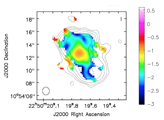
Figure 3: Spectral index map of A2495 between 5 GHz and 1.4 GHz. Countours are the same as the 1.4 GHz map, and typical errors range from $\Delta\alpha\simeq$ 0.2 to $\Delta\alpha\simeq$ 0.6 for the inner and outer regions, respectively.

The synchrotron index $\alpha$ is defined as:

$$\alpha=-\dfrac{log\frac{S_{1}}{S_{2}}}{log\frac{\nu_{1}}{\nu_{2}}}$$ (1)

where, in this work, $S_{1}$ and $S_{2}$ are, respectively the 5 GHz flux (hereafter $S_{C}$) and the 1.4 GHz flux (hereafter $S_{L}$), while $\nu_{1}$ and $\nu_{2}$ are the corresponding frequences. The radio galaxy core, often characterised by $\alpha\sim$ - 0.5, exhibits $\alpha\simeq$ - 0.9, while lobes reach $\alpha\simeq$ - 2. Table 3 summarizes the spectral index properties.

Region	$S_{C}\pm\Delta S_{C}$	$S_{L}\pm\Delta S_{L}$	$\alpha$ $\pm$ $\Delta\alpha$
	[mJy]	[mJy]
Peak	0.77 $\pm$ 0.06	2.20 $\pm$ 0.18	-0.79 $\pm$ 0.08
Extended(a)	1.60 $\pm$ 0.16	13.50 $\pm$ 1.08	-1.59 $\pm$0.08
Total	2.37 $\pm$ 0.19	15.70 $\pm$ 1.26	-1.39 $\pm$ 0.22

Table 3: The first column shows the flux values at 5 GHz, while the second displays the 1.4 GHz values. The third column presents the correspondent spectral index values.
(a): estimated subtracting the peak contribute from the total flux.

The mean index is - 1.39 $\pm$ 0.22, in agreement with Hogan et al. (2015), that determined $\alpha\simeq$ - 1.35, thus suggesting the presence of an old electronic population.

3 X-ray Analysis

3.1 Observation and data reduction

A2495 has been observed with the Chandra Advanced CCD Imaging Spectrometer S (ACIS-S) on 17/07/2012 (ObsID 12876, P.I. Gitti) for a total exposure of $\sim$ 8 ks. Data were reprocessed with CIAO 4.9 using CALDB 4.2.1. First, the Chandra_repro script performed the bad pixels removal and the instrument errors correction; afterwards, we removed the background flares and we used Blanksky background files, filtered and normalized to the count rate of the source hard X-ray image (9-12 keV), in order to subtract the background. The final exposure time is 7939 s.
We identified and removed point sources using the CIAO tool Wavdetect. Comparing X-ray sources with optical counterparts, we checked the astrometry of the Chandra data, and found it to be accurate; no registration correction was necessary. Unless otherwise stated, the reported errors are at 68$\%$ (1$\sigma$) confidence level.

3.2 Results

3.2.1 Surface Brightness Profile

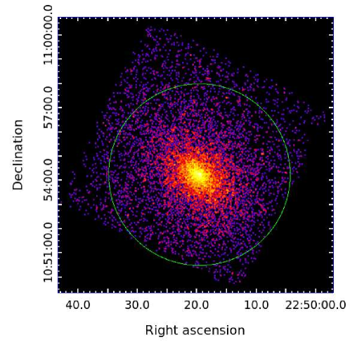
Figure 4: 0.5-2 keV image of A2495, smoothed with a 5$\sigma$ gaussian. The green circle represents the maximum radius considered for the spectral analysis (see Sec. 3.2.2).

Figure 4 shows the smoothed 0.5-2 keV image of A2495. We produced a background-subtracted, exposure-corrected image and then extracted the surface brightness profile from a series of 2^′′-width concentric annuli centered on the X-ray peak.
We used Sherpa in order to fit this profile in the outer radii ($\geq$ 30^′′) with a single $\beta$-model (Cavaliere & Fusco-Femiano, 1976), and then extrapolated it to the inner regions. The best-fit values are r0=15.9 $\pm$ 0.9 arcsec, beta=0.46 $\pm$ 0.01 and ampl=0.41 $\pm$ 0.02 counts s^-1 cm^-2 sr^-1; the ratio between the $\chi^{2}$ and the degrees of freedom (DoF) is $\chi^{2}/DoF\simeq$ 1.59. The result is represented with the blue line in Fig 5.

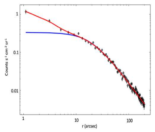
Figure 5: Surface brightness profile of A2495 fitted in the external regions ($\geq$ 30^′′) with a single $\beta$-model (blue line) and on every radius with a double $\beta$-model (red line). The blue line in the inner regions was obtained by extrapolating the model.

We can clearly note the brightness excess characterizing the central regions of cool-core clusters. We therefore fitted a double $\beta$-model (Mohr et al., 1999; LaRoque et al., 2006) on the entire radial range. In this case, the best-fit parameters are r0₁=2.74 ${}^{+4.55}_{-1.63}$ arcsec, beta₁=0.64 ${}^{+1.61}_{-0.25}$ and ampl₁=1.09 ${}^{+0.55}_{-0.24}$ counts s^-1 cm^-2 sr^-1 for the first and r0₂=20.3 ${}^{+6.1}_{-2.1}$ arcsec, beta₂=0.48 ${}^{+0.06}_{-0.01}$ and ampl₂=0.31 ${}^{+0.04}_{-0.11}$ counts s^-1 cm^-2 sr^-1 for the second $\beta$-Model. $\chi^{2}/DoF$ is 1.05. The corresponding model line is shown in red in Fig. 5. This suggests that A2495 is, indeed, a cool-core cluster, as expected from the selection criteria exploited for the cluster choice.

3.2.2 Spectral Analysis

We extracted and fitted spectra of A2495 in the 0.5-7 keV band via Xspec (vv.12.9.1), excluding data above 7.0 keV and below 0.5 keV in order to prevent, respectively, contamination from the background and calibration uncertainties. We derived the global cluster properties extracting a spectrum from a $\sim$ 200^′′ circular region centered on the X-ray peak (located at $RA$=22${}^{\text{h}}$50${}^{\text{m}}$19.4${}^{\text{s}}$, $DEC$=+10$\degree$54${}^{\text{m}}$14.2${}^{\text{s}}$). The spectrum was then fitted assuming an absorbed emission produced by a collisionally-ionized diffuse gas, making use of the wabs*apec model. The hydrogen column density was fixed at $N_{H}$ = 4.73 $\cdot$ 10²⁰ cm^-2 (estimated from Kalberla et al., 2005); redshift was fixed at $z$ = 0.07923. The only parameters left free to vary were the abundance $Z$, the temperature $kT$ and the normalization parameter. We found $kT$ = 3.90 $\pm$ 0.20 keV, $Z$ = 0.54 ${}^{+0.11}_{-0.10}$ Z_⊙ and $F$(0.5-7 keV) = 1.07 ${}^{+0.01}_{-0.02}\cdot$ 10^-11 erg s^-1 cm^-2, leading to a total luminosity in the 0.5-7 keV band of $L$(0.5-7 keV) = (1.44 $\pm\ 0.02$)$\ \cdot$ 10⁴⁴ erg s^-1.
We then performed a projected analysis, using a series of concentric rings covering the entire CCD and centered on the X-ray peak, each of which contains a minimum of 2500 total counts (the maximum radius reached, corresponding to 200^′′, is visible in Fig. 4). Results are listed in Table 4.

$r_{\text{min}}$-$r_{\text{max}}$	Counts	kT	Z	$\chi^{2}/Dof$
[arcsec]		[keV]	[Z⊙]
1.5 - 25.1	2230 (98.9 %)	3.35 ${}^{+0.43}_{-0.29}$	1.04 ${}^{+0.43}_{-0.31}$	53/67
25.1 - 47.2	2240 (97.4 %)	4.05 ${}^{+0.55}_{-0.48}$	0.57 ${}^{+0.41}_{-0.28}$	94/67
47.2 - 72.8	2002 (94.1 %)	4.09 ${}^{+0.54}_{-0.47}$	0.46 ${}^{+0.29}_{-0.24}$	67/61
72.8 - 100.4	1718 (89.6 %)	3.97 ${}^{+0.65}_{-0.58}$	0.34 ${}^{+0.32}_{-0.23}$	53/55
100.4 - 129.9	1513 (82.1 %)	4.75 ${}^{+1.20}_{-0.89}$	0.36 ${}^{+0.42}_{-0.35}$	36/49
129.9 - 157.4	1368 (76.7 %)	5.30 ${}^{+1.34}_{-1.05}$	0.82 ${}^{+0.81}_{-0.55}$	45/45
157.4 - 185.5	1151 (67.1 %)	5.01 ${}^{+2.07}_{-1.26}$	0.44 ${}^{+0.88}_{-0.44}$	29/39
185.5 - 214.0	1020 (56.6 %)	3.09 ${}^{+1.65}_{-0.86}$	6.4e-02	41/35

Table 4: Fit results of the projected radial analysis. The first column show the lower and upper limits of the extraction rings in arcsec, the second column represents the number of source photons coming from each ring, while the percentage indicates their number compared to the total photons of the same region. Finally, in the last three columns we report the values ​​of temperature, metallicity and $\chi^{2}/$ DoF, respectively.

The low statistics led to large uncertainties in the measured abundances; therefore, in this work the cluster metallicity will not be discussed.

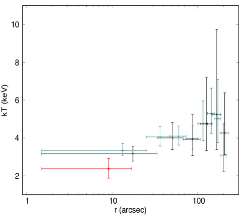
Figure 6: Projected (cyan) and deprojected (black) temperature profile of A2495. Bars in the x-axis represent the limits of the extraction rings, while the y-axis ones are the errors for the temperature values. The red point is derived from the spectral analysis described in Sec. 4.3.

The projected temperature profile of A2495 is shown in cyan in Fig 6. We carried out the same analysis making use of elliptical rings, but we did not find any significant difference.
In order to account for the projection effects, we performed a deprojection analysis by adopting the projct model. For this purpose, we used concentric rings containing at least 3500 total counts. Similarly as above, the X-ray peak was excluded. Spectra were fitted using a projct*wabs*apec model, in which temperature, abundance and normalization parameters were left free to vary. Results are listed in Table 5. The deprojected temperature profile of the cluster is shown in black in Fig 6.

$r_{min}$-$r_{max}$	Counts	kT	Z	N(r) (10-4)	Electronic Density	Pressure	tcool
[arcsec]		[keV]	[Z⊙]		[$10^{-2}\$cm-3]	[10-11 dy cm-2]	[Gyr]
1.5 - 33.5	3143 (98.7 %)	3.16 ${}^{+0.39}_{-0.38}$	1.09 ${}^{+0.57}_{-0.38}$	14.3 ${}^{+2.1}_{-2.1}$	1.30 ${}^{+0.03}_{-0.03}$	11.8 ${}^{+1.7}_{-1.7}$	4.0 ${}^{+0.6}_{-0.6}$
33.5 - 67.4	2945 (95.7 %)	4.00 ${}^{+0.80}_{-0.62}$	0.43 ${}^{+0.39}_{-0.31}$	21.0 ${}^{+2.5}_{-2.5}$	0.57 ${}^{+0.03}_{-0.03}$	6.8 ${}^{+1.7}_{-1.4}$	10.0 ${}^{+2.5}_{-2.0}$
67.4- 106.7	2430 (89 %)	3.92 ${}^{+1.30}_{-0.86}$	0.30 ${}^{+0.50}_{-0.30}$	17.5 ${}^{+2.8}_{-2.8}$	0.29 ${}^{+0.03}_{-0.03}$	3.3 ${}^{+1.4}_{-1.0}$	20.1 ${}^{+8.7}_{-6.4}$
106.7 - 146.1	2042 (80.2 %)	4.79 ${}^{+2.47}_{-1.41}$	0.32 ${}^{+0.85}_{-0.32}$	15.2 ${}^{+2.7}_{-3.3}$	0.18 ${}^{+0.03}_{-0.03}$	2.6 ${}^{+1.8}_{-1.2}$	34.0 ${}^{+22.6}_{-16.1}$
146.1 - 186.0	1709 (69.1 %)	5.19 ${}^{+4.50}_{-1.85}$	1.46 ${}^{+1.47}_{-1.47}$	8.7 ${}^{+3.7}_{-3.5}$	0.11 ${}^{+0.04}_{-0.03}$	1.6 ${}^{+1.9}_{-1.1}$	61.1 ${}^{+74.3}_{-42.2}$
186.0 - 225.8	1384 (56.3 %)	4.27 ${}^{+2.12}_{-1.13}$	0.16 ${}^{+0.54}_{-0.16}$	18.1 ${}^{+2.4}_{-2.9}$	0.12 ${}^{+0.02}_{-0.03}$	1.6 ${}^{+1.2}_{-0.7}$	46.9 ${}^{+32.4}_{-23.6}$

Table 5: Fit results of the deprojection analysis. The first two columns present, respectively, the limits of the annular regions and the number of source photons coming from each ring, while the percentage indicates their number compared to the total photons of the same region. The remaining columns report temperature, metallicity, normalization factor, electronic density, pressure and cooling time. The fit gives $\chi^{2}/$DoF = 394/437.

In both profiles, the temperature value rises, as expected, moving from the center to the outskirts. The outermost bin of the projected analysis suggests the decline typical of relaxed clusters (Vikhlinin et al., 2005). This is less pronounced in the deprojected profile, where the poor statistics led to larger errors.
The normalization factor $N$(r) of the apec model (see Table 5), if calculated through the deprojection analysis, allows us to obtain an estimate of the electronic density. It is defined as:

$$N(\text{r})=\dfrac{10^{-14}}{4\pi[D_{A}(1+z)]^{2}}\int n_{e}n_{p}dV$$ (2)

where $D_{A}$ is the angular distance of the source, calculated as $D_{A}=\dfrac{D_{L}}{(1+z)^{2}}$, $n_{e}$ represents the electronic density, $n_{p}$ the proton density and V is the shell volume. For a collisionally-ionized plasma (e.g., Gitti et al., 2012):

$$\int n_{e}n_{p}dV\simeq 0.82n_{e}^{2}V$$ (3)

The electronic density can therefore be estimated as:

$$n_{e}=\sqrt{10^{14}\bigg{(}\dfrac{4\pi\cdot N(r)\cdot[D_{A}\cdot(1+z)^{2}]}{0.82\cdot V}\bigg{)}}$$ (4)

Table 5 lists the density values for each shell. The corrisponding radial density profile is shown in Fig 7.

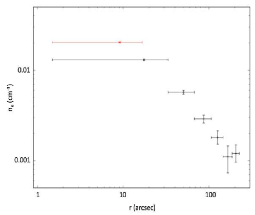
Figure 7: Density profile of A2495, obtained from the deprojection analysis. X-axis bars represent the limits of the extraction rings, while the y-axis ones are the errors estimated for the density. The red point is derived from the spectral analysis described in Sec. 4.3.

From the temperature and density profiles we estimated the cooling time of each region, defined as:

$$t_{\text{cool}}=\dfrac{H}{\Lambda(T)n_{e}n_{p}}=\dfrac{\gamma}{\gamma-1}\dfrac{kT(r)}{\mu Xn_{e}(r)\Lambda(T)}$$ (5)

where $\gamma$=5/3 is the adiabatic index, $H$ is the enthalpy, $\mu\simeq$ 0.61 is the molecular weight for a fully ionized plasma, $X$ $\simeq$ 0.71 is the hydrogen mass fraction and $\Lambda(T)$ is the cooling function (Sutherland & Dopita, 1993). Results are listed in Table 5, while the cooling time profile is shown in Fig. 8.
We adopted the definition of the cooling radius as the radius at which the cooling time is shorter than the age of the system. It is customary to assume the cluster’s age to be equal to the lookback time at $z$=1, since at this time many clusters appear to be relaxed: $t_{\text{age}}$ $\simeq$ 7.7 Gyr.

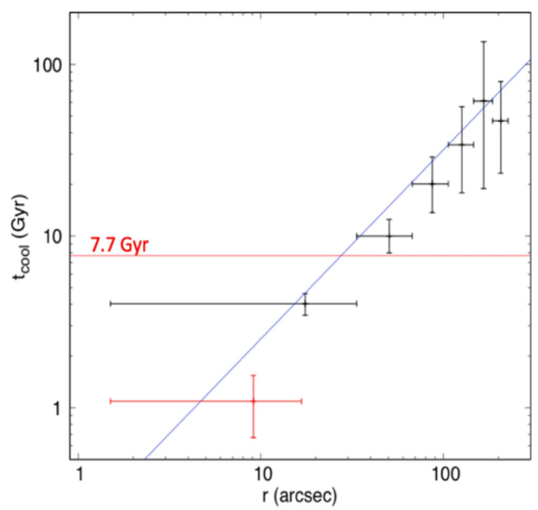
Figure 8: Cooling time profile for A2495. Each point represents the cooling time value for one of the annular regions used for the spectral extraction, and the x-axis errorbars are the lower and upper limits of each ring. The red line represents t${}_{\text{age}}$ = 7.7 Gyr, while the blue line is the best-fit of the profile: t${}_{\text{cool}}$=$0.199r^{1.102}$. The red point is derived from the spectral analysis described in Sec. 4.3.

We estimated for A2495 a cooling radius of:

$$r_{\text{cool}}\simeq(28\pm 16)\ \text{arcsec}\simeq(40\pm 23)\ \text{kpc}$$ (6)

In order to determine the X-ray luminosity produced within this radius ($L_{\text{cool}}$), we extracted a spectrum from a circular region with $r$ = $r_{\text{cool}}$ (excluding the central 1.5”) and fitted it with a wabs*apec model; Table 6 lists the results.

$r_{\text{min}}$-$r_{\text{max}}$	1.5 - 28.5	[arcsec]
Counts	2500(98.9 %)
kT	3.29 $\pm^{0.33}_{0.28}$	[keV]
Z	0.86 $\pm^{0.36}_{0.27}$	[Z⊙]
Flux${}_{\text{Bolo}}$	3.17	[10-12 erg s-1 cm-2]
Flux${}_{2-10\ \text{keV}}$	1.21	[10-12 erg s-1 cm-2]

Table 6: Fit results to the cooling region. The $\chi^{2}$/Dof is 68/74.

Therefore, the bolometric cooling luminosity is:

$$L_{\text{cool}}=4.3\ ^{+3.1}_{-3.4}\cdot 10^{43}\ \text{erg \ s}^{-1}$$ (7)

The same spectrum was fitted with a wabs*(apec+mkcflow) model; mkcflow adds an isobaric multi-phase component, allowing us to reproduce a cooling flow-like emission, while apec takes into account the background contribution. Temperature and abundance of the apec model were left free to vary; we bounded them to the high temperature and abundance parameter of mkcflow. Redshift and absorbing column density were fixed at the Galactic values (see above), while the low temperature parameter of mkcflow was fixed at $\sim$ 0.1 keV; in this way, we are assuming a standard cooling flow. The norm parameter of mkcflow provides an estimate of the Mass Deposition Rate of the cooling flow ($\chi^{2}$/DoF $\sim$ 68/73):

$$\dot{M}<7\ \text{M${}_{\odot}$ yr${}^{-1}$}$$ (8)

An alternative method to obtain an estimate of the mass accretion rate exploits the luminosity $L_{\text{cool}}$ associated with the cooling region, assuming that it is all due to the radiation of the total gas thermal energy plus the pdV work done on the gas as it enters the cooling radius. These assumptions are typical of the classical cooling flow model (Fabian et al., 1994), that does not take into consideration heating produced by the central AGN.

$${\dot{M}}\simeq\dfrac{2}{5}\dfrac{\mu m_{p}}{kT}\cdot L_{\text{cool}}\simeq 52\ ^{+38}_{-42}\ \text{M${}_{\odot}$ yr${}^{-1}$}$$ (9)

Finally, in Table 5 we list the pressure values calculated as $p=1.83n_{e}kT$, where $n_{e}$ was taken from the deprojection analysis. Fig. 9 shows the correspondent radial profile.

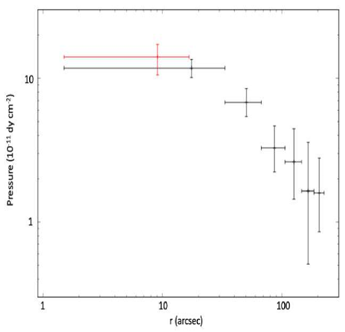
Figure 9: Pressure radial profile obtained from the deprojection analysis. The red point is derived from the spectral analysis described in Sec. 4.3.

4 Discussion

In Fig 10 we show the smoothed 0.5-2 keV image, with overlaid the 1.4 GHz contours, zoomed into the cluster center.

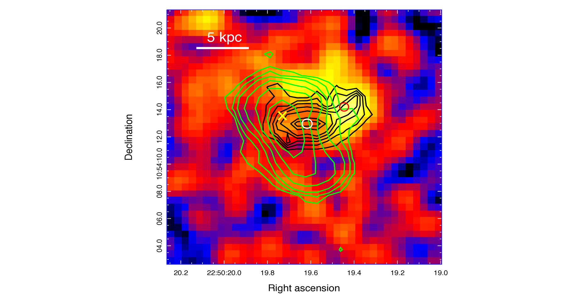
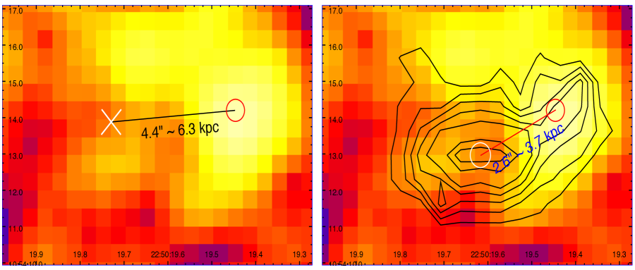
Figure 10: Top Panel: 1.4 GHz (green) and H$\alpha$ (black) contours overlaid on the 0.5-2 keV Chandra image of A2495. The red and white circles represent the X-ray and H$\alpha$ peaks, respetively, while the yellow cross is the position of the X-ray centroid. Bottom-Left Panel: Offset between the emission centroid (white cross) and the X-ray peak (red circle). Bottom-Right Panel: Offset between the H$\alpha$ (white circle) and the X-ray (red circle) peaks.

We highlight the presence of an offset between the BCG ($RA$=22${}^{\text{h}}$50${}^{\text{m}}$19.7${}^{\text{s}}$, $DEC$=+10$\degree$54${}^{\text{m}}$12.7${}^{\text{s}}$) and the X-ray peak (red circle); this suggests that there is a relative motion between them. By means of the X-ray isophotes, we estimated the centroid (bottom-left panel of Fig. 10, black circle), located at $RA$=22${}^{\text{h}}$50${}^{\text{m}}$19.7${}^{\text{s}}$, $DEC$=+10$\degree$54${}^{\text{m}}$13.8${}^{\text{s}}$. The determination was made calculating the centroid in several regions centered on the peak and with radii ranging from 50 to 200 kpc.

The offset approximately measures 4.4^′′ $\pm$ 1.0^′′, corresponding to 6.3 $\pm$ 1.4 kpc. We investigated the possibility of the presence of a point source in the position of the X-ray peak, that could bias its location, extracting a spectrum from a $\sim$ 10^′′ radius region centered on the peak. The radius was chosen in order to obtain enough statistics to produce a reliable fit. The spectrum was then fitted with two models: wabs*apec and wabs*(apec+powerlaw). The powerlaw component, added to model the point-source emission, has two parameters: the spectral index and a normalization factor. If a point source is present, we expect a significant improvement of the fit using the second model. The first produced $\chi^{2}/DoF$=42/54, while for the second $\chi^{2}/DoF$= 40/52. In order to determine if the distribution improved with the addition of the powerlaw emission, we applied the F-stat method, obtaining $P_{f}$=1.3, thus indicating that the addition of a second component is not statistically significant. We then performed a search by coordinates in X-ray, optical and infrared catalogues. However, the closest object seems to be an IR source (SSTSL2 J225019.00+105414.5) located more than 10 kpc ($\sim$ 7.5^′′) away from the peak; therefore, it can not represent its optical counterpart. We thus find no evidence of an X-ray point source at the position of the X-ray peak, and conclude that the offset is real.
We propose that this offset could be produced by sloshing, an oscillation of the ICM within the cluster potential well, generated from perturbations such as, for example, minor mergers. This mechanism is usually tied to the formation of cold fronts (Markevitch & Vikhlinin, 2007), discontinuities between the hot cluster atmosphere and a cooler region (i.e. the cooling center) that are moving with respect to each other. In this scenario, the oscillation of the ICM has displaced the X-ray peak from the cluster’s centre: the cooling process is not taking place on the BCG nucleus (see Sec. 1). However, deeper observations are necessary to test this hypothesis by means of detailed analysis of the thermodynamic properties of the galaxy cluster central regions.

4.1 H$\alpha$ emission analysis

The detection of line emitting nebulae in the proximity of BCGs is known to be an indicator of the presence of multiphase gas. Such structures are only found when the central entropy drops below 30 keV cm² or, equivalently, when t${}_{\text{cool}}\ <$ 5 $\cdot$ 10⁸ yr (e.g., Cavagnolo et al., 2008; McNamara et al., 2016). VIMOS (Visibile Imaging Multi-Object Spectrograph) observations of the H$\alpha$ line emission of a sample of 73 clusters, including A2495, were presented by Hamer et al. (2016). To be consistent with the multi-wavelength data shown in this work, we checked and corrected the astrometry exploiting the HST F606W image (see Sec. 4.2) and the F555W image that was used by Hamer et al. (2016) to align the VIMOS data, finding an offset of  1.3 arcsec between the BCG centroids in them. In Fig. 11 we show the astrometrically corrected H$\alpha$ image.

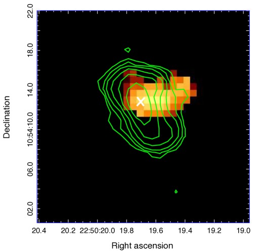
Figure 11: H$\alpha$ emission structure in the inner regions of A2495 observed by VIMOS (Hamer et al., 2016). The green radio contours are the same of Fig. 10 and units are in 10^-16 erg s^-1 cm^-2 Å^-1.

The total luminosity is (5.03 $\pm$ 0.81) $\cdot$ 10³⁹ erg s^-1. The structure is elongated on a scale of $\sim$ 5.6^′′ ($\sim$ 8 kpc). In Fig. 10 we show the H$\alpha$ emission contours (black) overlaid on the smoothed 0.5-2 keV image. The H$\alpha$ structure stretches towards and surrounds the X-ray peak, connecting it to the BCG. The same behaviour is found in other galaxy clusters (e.g., A1991, A3444 and RXJ0820.9+0752 in Hamer et al. 2012; Bayer-Kim et al. 2002, or A1111, A133, A2415 and others in Hamer et al. 2016), where the H$\alpha$ plume either follows the X-ray peak or acts like a bridge between the peak and the BCG. This could suggest that the line emission is not produced by ionisation coming from stellar radiation or from the AGN; in this scenario, in fact, one expects the emission to be associated with the BCG, rather than with the X-ray core (e.g., Hamer et al., 2016; Crawford et al., 2005). This 10⁴ K gas is therefore likely connected to the cooling ICM (e.g., Bayer-Kim et al., 2002; Canning et al., 2012; Crawford et al., 2005; Ferland et al., 2009). Moreover, we note that the A2495 line emission luminosity is significantly weaker (typically of about an order of magnitude) with respect to the plumed population presented in Hamer et al. (2016); this cluster could represent a lower luminosity limit of this sample.
We also highlight the presence of a further, less pronounced ($\sim$ 2.6^′′, corresponding to 3.7 kpc) offset between the H$\alpha$ and the X-ray peaks. We first checked if it could be produced by astrometric uncertainties. The VIMOS data were obtained with a seeing of 0.95^′′ (from Hamer et al., 2016), while the overall 90% uncertainty circle of Chandra X-ray absolute position has a radius of 0.8^′′. The upper limit of the astrometric uncertainty is thus expected to be $\Delta x_{tot}=\sqrt{\Delta x_{Chandra}^{2}+\Delta x_{VIMOS}^{2}}=1.24^{\prime\prime}\simeq 1.7\ \text{kpc}$; since our offset is larger ($\sim$ 3.6 kpc), it is likely to be a real feature.
We argue that this offset could originate to the different hydrodynamic conditions of the ICM: the H$\alpha$ emission is generated from $\sim 10^{4}$ K gas, $\sim 10^{2}-10^{3}$ denser than the surrounding hot ICM. Thus, hydrodynamic processes may lead to differential motion between these two phases and generate the offset. Another hypothesis is that thermal instabilities (or so-called precipitation) occurring in the inner regions of the cluster could have produced the $10^{4}$ K gas in situ, following the chaotic cold accretion scenario (CCA) (e.g., Gaspari et al., 2012; Voit et al., 2015, see Sec. 4.3).
In some cases (e.g., A1991, Hamer et al., 2012), two H$\alpha$ peaks, with one being coincident with the X-ray one, are detected. As this object does not show a second, or even dominant, peak of line emission at the X-ray peak, it is possible this represents an earlier stage of these offsets, one in which there has not yet been sufficient time for the cooled gas at the offset location to grow to a mass comparable to that already in the BCG. The plume of optical line emission shows a very clear velocity gradient (see Hamer et al. 2016 for further details), and as the ionised gas can be used as a direct tracer of the motion of the cold gas, can be used to study the dynamics of the cold gas during the sloshing process. Following the method of Hamer et al. (2012), we estimated the dynamical offset timescale of the cold gas. The plume extends for $\sim$ 8 kpc from the centre of the BCG (5.6 arcsec at 1.44 kpc/$"$), the gas velocity at the centre of the BCG is consistent with the stellar component to within 10 km $\cdot$ s^-1, indicating that the plume really extends out from the BCG and is not just a projection effect. The velocity of the gas changes smoothly and consistently along the plume, and we measured a velocity difference of $\sim$ +350 km between the gas at the end of the plume and at the centre of the BCG. Thus, we measured a projected extent D’ = 8 kpc = 2.47 $\cdot$ 10¹⁷ km and a projected velocity shift of V’ = +350 km $\cdot$ s^-1, indicating a projected timescale of T’ = D’/V’ = 7.05 $\cdot$ 10¹⁴ s or $\sim$ 22.4 Myr. To correct for the projection effects we must know the inclination of the offset (as T = T’ $\times$ cos[i]/sin[i]). While the inclination cannot be determined from the data in hand, the most likely inclination to expect is $\sim$ 60$\degree$ (Hamer et al., 2012), which would give an offset dynamical timescale of T$\sim$ 13 Myr.

4.2 Optical analysis

Deep optical images of the cluster galaxy were retrieved from the HST archive. We used HST ACS observations taken in the two wide filters F606W (V-band) and F814W (I-band). Images in these two filters have been instrumental in generating a dust extinction map and in the evaluation of the galaxy luminosity within the central 10kpc. In order to estimate the dust mass in the central region, we developed a 2-D galaxy model by fitting the starlight with elliptical isophotes in an iterative process with subsequent removal of sources in the field or by masking features not related to the stellar light distribution. An extinction map $A_{V}=-2.5~{}log(I_{obs}/I_{model})$ (Fig. 12) was generated from the observed intensity $(I_{obs})$ and the intensity of the starlight model $(I_{model})$ . To avoid the introduction of artifacts in the final map, particular care has been taken in the generation of the starlight model in the central few arc seconds, where a dust lane crosses the galactic center, making the isophote fitting process quite challenging.

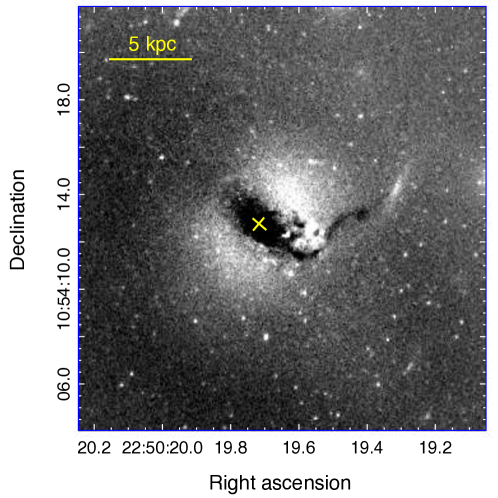
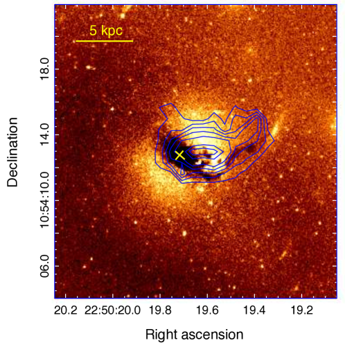
Figure 12: Left panel: Dust extinction map of the BCG and core of A2495, obtained from the F606W HST image. Dust in absorption, seen as a filamentary structure, encircles the inner region of the galaxy and stretches towards the outskirts. Right panel: H$\alpha$ contours overlaid on the dust extinction map. The two structures are co-spatial.

The extinction map confirms that an highly absorbed dust lane crosses the galaxy center, while a large wavy filamentary structure extends to the West for about $4^{\prime\prime}$. Additional knots of highly absorbed dust are apparent in the central kpc of the galaxy. Although the peak of the warm ionized gas does not correspond to the galactic center or any other location of high extinction, the lower ridge of the H$\alpha$ emission seems to be associated with dust absorption revealed in the filamentary structure.
Dust structures are common in BCGs. Van Dokkum & Franx (1995) detected dust in 50% of the galaxies included in their sample of 64 objects; Laine et al. (2003) found signs of dust absorption in 38% of 81 BCGs, classifying them, according to their morphology, into nuclear dust disk, filaments, patchy dust, dust rings and dust spirals (see Section 3.2 and Fig. 3 of Laine et al. 2003 for further details). The structure in A2495 seems to fall into the second class, looking like a classic dust filament. The BCG of this cluster was also part of the large Spitzer dust survey presented by Quillen_2008 and discussed in O'Dea_2008; these studies highlighted that dust in A2495 does not show a particularly remarkable mid-IR continuum and is not detected at 70 $\mu$m, likely suggesting that the star formation does not significantly heat the dust as it is, instead, seen in other systems (see Quillen_2008 for more details).
From the extinction map we calculated the total dust mass in the central 7 kpc under some basic assumptions for the grain size distribution and composition. The approach and relative calculations are outlined in Goudfrooij et al. (1994); here we assume dust extinction properties similar to what is observed in the Milky Way. We used a grain size distribution proportional to a^-3.5 (where a is the grain radius) (Mathis et al., 1977; Goudfrooij et al., 1994) and a mixture of graphite and silicate (equal absorption from those) with a specific grain mass density of 3 g/cm³. Lower and upper limits for the grain size distribution were set to $a_{-}=0.005~{}\mu$m and $a_{+}=0.22~{}\mu$m (Draine & Lee, 1984). The filamentary structure was divided into 5 sectors, as shown in Fig. 13.

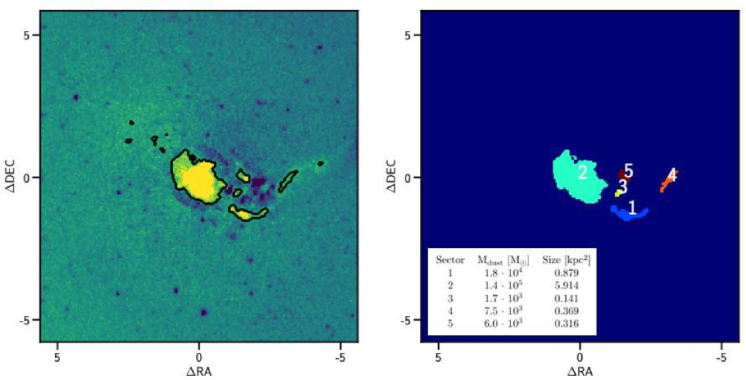
Figure 13: Sectors in which the dust mass estimation was performed. The table shows the dust mass values and the size for each sector. .

The total dust mass accounted in all the filamentary structures in the central 7 kpc is $1.7\cdot 10^{5}$ M_☉. The reported mass should be regarded as lower limit, considering that the method used in generating the extinction map would mask a centrally symmetric diffuse dust component, if present. Given the uncertainties in the generation of an accurate galaxy model at the galactic center and the statistical error, we estimate a 30% uncertainty in the reported dust mass. We remark that the optically detected dust likely underestimates the total dust content (see for example Temi et al., 2004, for a study of dust in a sample of elliptical galaxies).
Assuming a dust/gas ratio of $M_{\text{dust}}/M_{\text{gas}}\sim 1/100$ (e.g., Edge_2010), we expect for A2495 a minimum cold gas mass within the central 7 kpc of $\sim$ 2 $\cdot$ 10⁷ M_☉ (again, with a 30% uncertainty). We note that the mass of the H$\alpha$-emitting gas within the same region (assuming that it is optically thin and in pressure equilibrium with the local ICM) is:

$$M_{\text{H$\alpha$}}\simeq L_{\text{H$\alpha$}}\dfrac{\mu m_{p}}{n_{\text{H$\alpha$}}\epsilon_{\text{H$\alpha$}}}$$ (10)

where $L_{\text{H}\alpha}$ is that reported in Sec. 4.1 and $\epsilon_{\text{H}\alpha}\sim 3.3\cdot 10^{-25}$ erg cm³ s^-1 is the H$\alpha$ line emissivity; $n_{\text{H$\alpha$}}$ is obtained assuming:

$$n_{\text{H$\alpha$}}T_{\text{H$\alpha$}}\simeq n_{\text{ICM}}T_{\text{ICM}}$$ (11)

where $T_{\text{H$\alpha$}}\sim 10^{4}$ K, $T_{\text{ICM}}$ is the first value reported in Tab. 8 (since the H$\alpha$ structure is located within the central 7 kpc), while $n_{\text{ICM}}\sim 1.83n_{e}$. Again, $n_{e}$ can be retrieved from Tab. 8. We thus obtain $M_{\text{H$\alpha$}}\sim 10^{5}\pm 10^{4}$ M_⊙.
The H$\alpha$ mass can account for just a negligible fraction of the total cold gas mass estimated above: a significant amount is still missing. We speculate that colder, likely molecular gas is present in the central regions of A2495. This is supported by the correlation between the H$\alpha$ luminosity and the molecular mass (Edge, 2001; Pulido et al., 2018), from which we obtain $M_{\text{mol}}\sim$ 10⁹ M_☉. The contrast with the estimate determined from the dust/gas ratio is only apparent: the latter takes into account the dust mass within the central 7 kpc of the BCG and constitutes, per se, a lower limit (see above). Cold molecular gas could also lie offset from the BCG, as observed in other systems where evidence for CO line emission coincident with the offset X-ray peak was detected (e.g., Hamer et al., 2012).

4.3 Does sloshing regulate the generation of multiple cavity systems?

We investigated the presence of cavities in A2495 by considering a residual image obtained by subtracting a 2-D $\beta$-Model from the 0.5-2 keV image. The result is shown in Fig. 14.

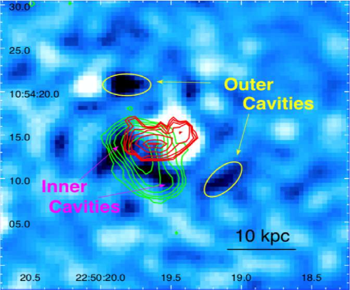
Figure 14: Residual image showing the two cavity systems located in A2495. The first pair is coincident with the radio lobes, while the second is symmetrical with respect to the X-ray peak region. The H$\alpha$ contours are overlaid in red, while the green contours are the same of Fig 10.

We notice an X-ray blob surrounding the peak region and four ICM depressions (two pairs), corresponding to $\sim$30$\%$ (at 90$\%$ confidence level) surface brightness deficits. Although we are aware of the limitations of our snapshot exposure, we notice that their shape and position, symmetrical with respect to the BCG for the first pair and to the X-ray peak for the second one(see Fig. 14), suggest that they could be real structures. In the following analysis and discussion, we assume them as cavities. However, it is possible that the poor statistic could have led to the production of artifacts; the reader shall thus be warned about the significance of these depressions. Deeper observations are therefore required to confirm their significance.
The first pair seems to be coincident with the radio galaxy lobes, while the second pair is centered on, and falls on opposite sides of, the X-ray excess. Hereafter, we will refer to them as, respectively, inner and outer cavities. We also assume that cavities belonging to the same pair are characterised by the same elliptical shape and dimensions. Table 7 lists their properties (a refers to the major axis, b to the minor one).

Cavity	a	b	V	R
	[kpc]	[kpc]	[kpc3]	[kpc]
Inner	6.8	2.9	70.3	4.9
Outer	8.0	4.9	164.0	11.9

Table 7: Properties of the two cavities systems of A2495. a and b are the major and minor axis, V is the volume (estimated assuming an oblate elissoidal shape) while R is their distance from the BCG center.

Following the method described in Bîrzan et al. (2004), the cavity power can be estimated as:

$$P_{\text{cav}}=\dfrac{E_{\text{cav}}}{t_{\text{cav}}}=\dfrac{4pV}{t_{\text{cav}}}$$ (12)

where $t_{\text{cav}}$ is the age of the cavity. In order to obtain an estimate of the temperature closer to the cavities’ region, we performed a deprojection analysis with annular regions containing a minimum of 1500 counts; in fact, lowering the counts lower limit makes the rings radius smaller, bringing to a more localized estimate of the thermodynamical properties, albeit with larger uncertainties. However, we note that since we are close to the X-ray peak, the photon statistics remains high enough to obtain a good fit. We fitted a project*wabs*apec model and obtained the $kT$ value; results for the inner region, that corresponds to the radius we are interested in, are represented with a red dot in Fig. 6, 7, 8 and 9.
Density was, instead, obtained exploiting the surface brightness profile showed in Fig. 5. In fact, fitting a double $\beta$-Model on it (for details of this method, see Ettori et al., 2002) allows us to obtain an estimate for the density values for smaller radii with respect to the spectral analysis performed above. Results are shown in Fig. 15.

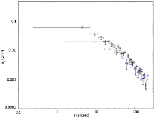
Figure 15: The black data are the results obtained from the double $\beta$-Model fit on the surface brightness profile, while the blue data are the results obtained from the spectral analysis described above.

Since the two cavity systems lies at, respectively, $\sim$ 4.9 kpc and $\sim$ 11.9 kpc from the cluster center (see Table 7), we will make use of the first two density values: the first will be used for the inner cavities, the second for the outer ones. The kT estimated above will instead be exploited for both the systems, since the current statistics does not allow us to provide more localized values. In Table 8 we finally report temperatures, densities and pressures used for the estimate of the cavities’ properties.

$r_{min}$ - $r_{max}$	kT(a)	$n_{e}$(b)	p
[arcsec]	[keV]	[10-2 cm-3]	[10-11 dy cm-2]
0.2 - 7	2.37 ${}^{+0.64}_{-0.55}$	6.49 ${}^{+0.59}_{-0.45}$	45.0 ${}^{+14.3}_{-12.6}$
7 - 11.5	2.37 ${}^{+0.64}_{-0.55}$	3.83 ${}^{+0.22}_{-0.47}$	26.6 ${}^{+7.6}_{-8.9}$

Table 8: Thermodynamical properties of the inner regions obtained from the deprojection analysis with 1500 counts ($\chi^{2}/$DoF $\sim$ 450/441) and from the fit of the surface brightness profile. The results of the spectral analysis are represented with red dots in Fig. 6, 7, 8 and 9.
(a) : obtained from the spectral analysis. (b) : obtained from the surface brightness profile.

		Sound velocity			Buoyancy velocity
	$c_{s}\ [$km s${}^{-1}]$	Age [Myr]	Pcav [1042 erg s-1]	$v\ [$km s${}^{-1}]$	Age [Myr]	Pcav [1042 erg s-1]
Inner	790 ${}^{+105}_{-83}$	6.0 ${}^{+0.8}_{-0.6}$	18.3 ${}^{+7.5}_{-6.6}$	259 $\pm$ 58	18 $\pm$ 4	6.0 ${}^{+2.3}_{-2.1}$
Outer	790 ${}^{+105}_{-83}$	14.4 ${}^{+1.7}_{-1.5}$	10.4 ${}^{+3.7}_{-4.1}$	214 $\pm$ 42	53 $\pm$ 11	2.8 ${}^{+0.9}_{-1.1}$

Table 9: Cavity velocity, age and power estimated with both the methods described in the text.

The cavity age was calculated as $t_{\text{cav}}=R/v$, where R is that defined in Table 7, while v is the cavity velocity. In this work, we will consider the sound and the buoyancy velocity. The latter is defined as:

$$v_{\text{buoy}}=\sqrt{\dfrac{2gV}{CA}}$$ (13)

where $C$ $\simeq$ 0.75 represents the drag coefficient, V and A are, respectively, the volume and the area of each cavity, while g is the gravitational acceleration.
We estimated the latter by making use of the galaxy luminosity profile (see Appendix) and of a simple model for the dark matter halo. We adopted a stellar $M/L_{\text{V}}\sim 4$, appropriate for an old stellar population with $\sim$ solar abundance (es. Maraston, 2005). The resulting stellar masses within the region of the inner and outer cavities are $M_{\text{BCG}}$($r\ <$ 4.9 kpc) $\sim 8.8\cdot 10^{10}$ M_⊙ and $M_{\text{BCG}}$($r\ <$ 11.9 kpc) $\sim 2.3\cdot 10^{11}$ M_⊙, respectively. Given the uncertainty on the mass-to-light ratio we adopted for these values a 30% error.
We estimated the dark matter contribution by assuming a NFW halo (Navarro et al., 1996) of mass $M_{\text{NFW}}=3.8\cdot 10^{14}$ M_⊙, estimated from the $M-T$ relation of Finoguenov et al. 2001, and a concentration $c=4.65$ (Prada et al., 2012; Merten et al., 2015). We note that the assumed mass is somewhat larger than the richness-based estimate by Andreon 2016 ($\sim 1.6\cdot 10^{14}M_{\sun}$). On the other hand, it is consistent with the hydrostatic mass (e.g., Gitti et al., 2012) determined exploiting the $\beta$-model (presented in Sec. 3.2.1), that returns $M\sim 3.2\cdot 10^{14}$ M_⊙. However, the conclusions for the cavity dynamics discussed below are quite insensitive to the precise values of $M_{\text{NFW}}$ and $c$. This model estimates dark masses of $M_{\text{DM}}(r<4.9$ kpc$)=3.3\cdot 10^{10}$ M_⊙ and $M_{\text{DM}}(r<11.9$ kpc$)=1.8\cdot 10^{11}$ M_⊙.
We therefore obtain a total mass within the central 4.9 kpc of $M_{\text{tot}}$($r\ <$ 4.9 kpc) $\sim 1.2\cdot 10^{11}$ M_⊙, while $M_{\text{tot}}$ ($r\ <$ 11.9 kpc) $\sim 4.1\cdot 10^{11}$ M_⊙. Results of the cavity analysis are listed in Table 9.
It is plausible that we are observing two different generations of cavities; the outer ones are older, while the inners probably still lie in the same regions they formed in. From this, we can infer that some process is probably switching the radio galaxy on and off: after the first generation forms, the AGN turns off and the cavities start to rise in the cluster atmosphere by buoyancy. Eventually, the AGN turns on again and another generation can be formed.
Following the CCA, cold gas could originate if thermal instabilities ensue (e.g., Gaspari et al., 2012). According to Voit et al. (2015), this is likely to happen when $t_{\text{cool}}/t_{\text{ff}}\leq 10-20$, where $t_{\text{ff}}=\sqrt{2R^{3}/GM}$ is the free-fall time. We note that, with the cooling time profile in Fig. 8 and the masses estimated above, this condition is not verified in A2495. However, McNamara et al. (2016) proposes that the $t_{\text{cool}}/t_{\text{ff}}$ ratio could be almost entirely governed by the cooling time. In both these interpretations, the cold gas could then accrete onto the SMBH efficiently and activate it.
We propose that in A2495 the sloshing process mentioned above could, as well, play a part in the feedback cycle. When the cooler region approaches the BCG, the AGN begins to accrete and turns on, producing the first generation of cavities. Subsequently, because of sloshing, the accreting material diminishes and the SMBH is switched off. The oscillation could, at a later time, make the process to repeat. This would produce different generations of cavities.
In order to investigate this scenario, we determined the free-fall time of the cooler region and compared it with the age difference of the two cavity generations, estimated with both the methods seen above. We obtained:

$$\normalsize\begin{cases}t_{\text{ff}}\simeq 15.4\pm 5.7\ \text{Myr}\\ \Delta t_{\text{cav}}^{\text{sound}}\simeq 8.4\ ^{+2.1}_{-1.8}\ \text{Myr}\\ \Delta t_{\text{cav}}^{\text{buoy}}\simeq 35\pm 12\ \text{Myr}\end{cases}$$ (14)

We thus estimate $\Delta t_{\text{cav}}\simeq t_{\text{ff}}$ : the age difference between cavities reflects the time scale needed for the cooling region to move towards the BCG and activate the AGN. This is also consistent with the dynamical timescale obtained in Sec. 4.1, that provides an alternative estimate for the offset lifetime.
Future works, exploiting deeper observations, will likely be able to confirm or disprove our hypothesis.

4.4 Can offset cooling affect the feedback process?

As we showed in the previous sections, the existing data suggest that cooling deposits gas away from the BCG nucleus so it cannot fuel the AGN. Therefore, we aim at investigating whether this can break the feeding-feedback cycle in A2495, or if the AGN activation cycle is driven by the periodicity of the gas sloshing motions.
We thus compared the power of the two putative cavity systems with the data available from samples of these structures (Bîrzan et al., 2017). The result is presented in Fig. 16, with the x axis representing the luminosity emitted within the cooling radius (estimated in Section 3.2.2). For the cavity power, we used the values obtained from the buoyancy velocity, for consistency with the work cited above.

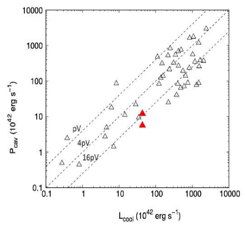
Figure 16: Black triangles represents the data from Bîrzan et al. (2017), while in red are the values for the two putative cavity systems considered in this work.

The values we estimated for A2495 are in good agreement with the global scatter of the observed relation. Therefore, we can argue that offset cooling seems to not break the feedback cyle, despite the evidence that cooling is not currently depositing gas into the BCG core where it can feed the AGN. Nevertheless, as we argued above, offsets probably still play a significant role in in the cycle regularization.

5 Conclusions

We carried out a thorough analysis of the X-ray and radio properties of A2495, by means of new observations requested with the purpose of performing a combined EVLA/Chandra study of this cool-core galaxy cluster. We also discussed H$\alpha$ emission data from Hamer et al. (2016) and exploited optical images retrieved from the HST archive. Our main results can be summarized as follows:

• The radio analysis at 1.4 and 5 GHz presented a small ($\sim$ 13-15 kpc) FRI radio galaxy with $L(1.4\ \text{GHz})\sim 2\cdot 10^{23}$ W Hz^-1 and no apparent diffuse emission. This places A2495 as having the least radio powerful BCG among the 13 BCS objects that meet our selection criteria. The spectral index map highlighted a very steep synchrotron spectrum ($\alpha\simeq 1.35$), suggesting the presence of an old electronic population.

• The X-ray study allowed us, through a deprojection analysis, to estimate the cooling radius of the cluster ($\sim$ 28^′′, corresponding to 40 kpc) and its luminosity (4.3 $\cdot 10^{43}$ erg s^-1). Furthermore, we determined the cooling time, the density and the pressure radial profiles, finding $t_{\text{cool}}<1$ Gyr inside $\sim 20$ kpc.

• The multi-wavelength analysis showed two significant offsets, one of $\sim$ 6 kpc between the emission centroid and the X-ray peak, while the other one ($\sim$ 4 kpc) between the X-ray and the H$\alpha$ peaks. We propose that the first could be produced by sloshing of the ICM, while the second still remains unexplained and is worthy of more investigations. The line emitting plume connects the X-ray core emission to the BCG, suggesting that the origin of the 10⁴ K gas could be linked to the cooling ICM. We found two putative cavity systems, the inner one with $t_{\text{age}}\sim 18$ Myr and $P_{\text{cav}}\sim$ 1.2 $\cdot$ 10⁴³ erg s^-1, while for the outer one $t_{\text{age}}\sim 53$ Myr and $P_{\text{cav}}\sim$ 5.6 $\cdot$ 10⁴² erg s^-1. Their age difference is consistent with the free-fall time of the central cooling gas and with the offset dynamical timescale estimated from the line emitting gas; we thus suggest that the same sloshing motions could switch the AGN on and off, forming different generations of cavities.

• Exploiting HST images, we located a dust lane crossing the BCG core in the North-South direction, and a $\sim$ 4^′′ filament extending West; we determined the dust mass within the central 7 kpc, finding $\sim$$1.7\cdot 10^{5}$ M_☉. We estimated in this region a lower limit for the total gas mass of $\sim$ 10⁷ M_⊙, and argued that, since the H$\alpha$ structure can not entirely account for it, a significant fraction is still missing. We propose that this fraction consists primarly of molecular gas; the $L_{\text{H}\alpha}$-$M_{\text{mol}}$ correlation supports this hypothesis, providing an estimate of $M_{\text{mol}}\sim 10^{9}$ M_☉.

• Finally, we proved that the offset cooling we found does not break the feedback cycle, since the cavity power values for A2495 with respect to the cooling luminosity are in agreement, within the scatter, with the observed $P_{\text{cav}}-L_{\text{cool}}$ correlation.

Deeper multi-wavelength observations (e.g., Chandra, ALMA) will be required in order to better investigate the hypothesis we made in this work. A similar combined analysis of the other 12 BCS clusters which meet our selection criteria, and that apparently show similar features, will provide a better understanding of these dynamically active environments.

References

- Anders & Grevesse (1989) Anders, E., & Grevesse, N. 1989, Geochim. Cosmochim. Acta, 53, 197, doi: 10.1016/0016-7037(89)90286-X
- Andreon (2016) Andreon, S. 2016, A&A, 587, A158, doi: 10.1051/0004-6361/201526852
- Bayer-Kim et al. (2002) Bayer-Kim, C. M., Crawford, C. S., Allen, S. W., Edge, A. C., & Fabian, A. C. 2002, MNRAS, 337, 938, doi: 10.1046/j.1365-8711.2002.05969.x
- Bîrzan et al. (2017) Bîrzan, L., Rafferty, D. A., Brüggen, M., & Intema, H. T. 2017, MNRAS, 471, 1766, doi: 10.1093/mnras/stx1505
- Bîrzan et al. (2004) Bîrzan, L., Rafferty, D. A., McNamara, B. R., Wise, M. W., & Nulsen, P. E. J. 2004, ApJ, 607, 800, doi: 10.1086/383519
- Canning et al. (2012) Canning, R. E. A., Russell, H. R., Hatch, N. A., et al. 2012, MNRAS, 420, 2956, doi: 10.1111/j.1365-2966.2011.20116.x
- Cavagnolo et al. (2008) Cavagnolo, K. W., Donahue, M., Voit, G. M., & Sun, M. 2008, ApJ, 683, L107, doi: 10.1086/591665
- Cavaliere & Fusco-Femiano (1976) Cavaliere, A., & Fusco-Femiano, R. 1976, A&A, 49, 137
- Crawford et al. (1999) Crawford, C. S., Allen, S. W., Ebeling, H., Edge, A. C., & Fabian, A. C. 1999, MNRAS, 306, 857, doi: 10.1046/j.1365-8711.1999.02583.x
- Crawford et al. (2005) Crawford, C. S., Hatch, N. A., Fabian, A. C., & Sand ers, J. S. 2005, MNRAS, 363, 216, doi: 10.1111/j.1365-2966.2005.09463.x
- Cui et al. (2016) Cui, W., Power, C., Biffi, V., et al. 2016, MNRAS, 456, 2566, doi: 10.1093/mnras/stv2839
- Donzelli et al. (2011) Donzelli, C. J., Muriel, H., & Madrid, J. P. 2011, The Astrophysical Journal Supplement Series, 195, 15, doi: 10.1088/0067-0049/195/2/15
- Draine & Lee (1984) Draine, B. T., & Lee, H. M. 1984, ApJ, 285, 89, doi: 10.1086/162480
- Ebeling et al. (1998) Ebeling, H., Edge, A. C., Bohringer, H., et al. 1998, MNRAS, 301, 881, doi: 10.1046/j.1365-8711.1998.01949.x
- Edge (2001) Edge, A. C. 2001, MNRAS, 328, 762, doi: 10.1046/j.1365-8711.2001.04802.x
- Ettori et al. (2002) Ettori, S., De Grandi, S., & Molendi, S. 2002, A&A, 391, 841, doi: 10.1051/0004-6361:20020905
- Fabian (2012) Fabian, A. C. 2012, ARA&A, 50, 455, doi: 10.1146/annurev-astro-081811-125521
- Fabian et al. (1994) Fabian, A. C., Canizares, C. R., & Boehringer, H. 1994, ApJ, 425, 40, doi: 10.1086/173959
- Fabian et al. (2006) Fabian, A. C., Sanders, J. S., Taylor, G. B., et al. 2006, MNRAS, 366, 417, doi: 10.1111/j.1365-2966.2005.09896.x
- Feretti & Giovannini (2008) Feretti, L., & Giovannini, G. 2008, in , 143–+
- Ferland et al. (2009) Ferland, G. J., Fabian, A. C., Hatch, N. A., et al. 2009, MNRAS, 392, 1475, doi: 10.1111/j.1365-2966.2008.14153.x
- Finoguenov et al. (2001) Finoguenov, A., Arnaud, M., & David, L. P. 2001, ApJ, 555, 191, doi: 10.1086/321457
- Gaspari et al. (2011) Gaspari, M., Melioli, C., Brighenti, F., & D’Ercole, A. 2011, MNRAS, 411, 349, doi: 10.1111/j.1365-2966.2010.17688.x
- Gaspari et al. (2013) Gaspari, M., Ruszkowski, M., & Oh, S. P. 2013, MNRAS, 432, 3401, doi: 10.1093/mnras/stt692
- Gaspari et al. (2012) Gaspari, M., Ruszkowski, M., & Sharma, P. 2012, ApJ, 746, 94, doi: 10.1088/0004-637X/746/1/94
- Gaspari et al. (2018) Gaspari, M., McDonald, M., Hamer, S. L., et al. 2018, ApJ, 854, 167, doi: 10.3847/1538-4357/aaaa1b
- Gitti et al. (2012) Gitti, M., Brighenti, F., & McNamara, B. R. 2012, Advances in Astronomy, 2012, doi: 10.1155/2012/950641
- Goudfrooij et al. (1994) Goudfrooij, P., de Jong, T., Hansen, L., & Norgaard-Nielsen, H. U. 1994, MNRAS, 271, 833, doi: 10.1093/mnras/271.4.833
- Graham et al. (2005) Graham, A. W., Driver, S. P., Petrosian, V., et al. 2005, AJ, 130, 1535, doi: 10.1086/444475
- Hamer et al. (2012) Hamer, S. L., Edge, A. C., Swinbank, A. M., et al. 2012, MNRAS, 421, 3409, doi: 10.1111/j.1365-2966.2012.20566.x
- Hamer et al. (2016) —. 2016, MNRAS, 460, 1758, doi: 10.1093/mnras/stw1054
- Heckman et al. (1989) Heckman, T. M., Baum, S. A., van Breugel, W. J. M., & McCarthy, P. 1989, ApJ, 338, 48, doi: 10.1086/167181
- Hogan et al. (2015) Hogan, M. T., Edge, A. C., Hlavacek-Larrondo, J., et al. 2015, MNRAS, 453, 1201, doi: 10.1093/mnras/stv1517
- Hogan et al. (2017) Hogan, M. T., McNamara, B. R., Pulido, F. A., et al. 2017, ApJ, 851, 66, doi: 10.3847/1538-4357/aa9af3
- Hudson et al. (2010) Hudson, D. S., Mittal, R., Reiprich, T. H., et al. 2010, A&A, 513, A37, doi: 10.1051/0004-6361/200912377
- Kalberla et al. (2005) Kalberla, P. M. W., Burton, W. B., Hartmann, D., et al. 2005, A&A, 440, 775, doi: 10.1051/0004-6361:20041864
- Katayama et al. (2003) Katayama, H., Hayashida, K., Takahara, F., & Fujita, Y. 2003, ApJ, 585, 687, doi: 10.1086/346126
- Laine et al. (2003) Laine, S., van der Marel, R. P., Lauer, T. R., et al. 2003, AJ, 125, 478, doi: 10.1086/345823
- LaRoque et al. (2006) LaRoque, S. J., Bonamente, M., Carlstrom, J. E., et al. 2006, ApJ, 652, 917, doi: 10.1086/508139
- Mann & Ebeling (2012) Mann, A. W., & Ebeling, H. 2012, MNRAS, 420, 2120, doi: 10.1111/j.1365-2966.2011.20170.x
- Maraston (2005) Maraston, C. 2005, MNRAS, 362, 799, doi: 10.1111/j.1365-2966.2005.09270.x
- Markevitch & Vikhlinin (2007) Markevitch, M., & Vikhlinin, A. 2007, Phys. Rep., 443, 1, doi: 10.1016/j.physrep.2007.01.001
- Mathis et al. (1977) Mathis, J. S., Rumpl, W., & Nordsieck, K. H. 1977, ApJ, 217, 425, doi: 10.1086/155591
- McDonald et al. (2010) McDonald, M., Veilleux, S., Rupke, D. S. N., & Mushotzky, R. 2010, ApJ, 721, 1262, doi: 10.1088/0004-637X/721/2/1262
- McDonald et al. (2014) McDonald, M., Swinbank, M., Edge, A. C., et al. 2014, ApJ, 784, 18, doi: 10.1088/0004-637X/784/1/18
- McNamara & Nulsen (2007) McNamara, B. R., & Nulsen, P. E. J. 2007, ARA&A, 45, 117, doi: 10.1146/annurev.astro.45.051806.110625
- McNamara et al. (2016) McNamara, B. R., Russell, H. R., Nulsen, P. E. J., et al. 2016, ApJ, 830, 79, doi: 10.3847/0004-637X/830/2/79
- McNamara et al. (2000) McNamara, B. R., Wise, M., Nulsen, P. E. J., et al. 2000, ApJ, 534, L135, doi: 10.1086/312662
- Merten et al. (2015) Merten, J., Meneghetti, M., Postman, M., et al. 2015, ApJ, 806, 4, doi: 10.1088/0004-637X/806/1/4
- Mittal et al. (2009) Mittal, R., Hudson, D. S., Reiprich, T. H., & Clarke, T. 2009, A&A, 501, 835, doi: 10.1051/0004-6361/200810836
- Mohr et al. (1999) Mohr, J. J., Mathiesen, B., & Evrard, A. E. 1999, ApJ, 517, 627, doi: 10.1086/307227
- Navarro et al. (1996) Navarro, J. F., Frenk, C. S., & White, S. D. M. 1996, ApJ, 462, 563, doi: 10.1086/177173
- Owen & Ledlow (1997) Owen, F. N., & Ledlow, M. J. 1997, The Astrophysical Journal Supplement Series, 108, 41, doi: 10.1086/312954
- Patel et al. (2006) Patel, P., Maddox, S., Pearce, F. R., Aragón-Salamanca, A., & Conway, E. 2006, MNRAS, 370, 851, doi: 10.1111/j.1365-2966.2006.10510.x
- Peterson & Fabian (2006) Peterson, J. R., & Fabian, A. C. 2006, Phys. Rep., 427, 1, doi: 10.1016/j.physrep.2005.12.007
- Prada et al. (2012) Prada, F., Klypin, A. A., Cuesta, A. J., Betancort-Rijo, J. E., & Primack, J. 2012, MNRAS, 423, 3018, doi: 10.1111/j.1365-2966.2012.21007.x
- Pulido et al. (2018) Pulido, F. A., McNamara, B. R., Edge, A. C., et al. 2018, ApJ, 853, 177, doi: 10.3847/1538-4357/aaa54b
- Rafferty et al. (2006) Rafferty, D. A., McNamara, B. R., Nulsen, P. E. J., & Wise, M. W. 2006, ApJ, 652, 216, doi: 10.1086/507672
- Rau & Cornwell (2011) Rau, U., & Cornwell, T. J. 2011, A&A, 532, A71, doi: 10.1051/0004-6361/201117104
- Rines et al. (2016) Rines, K. J., Geller, M. J., Diaferio, A., & Hwang, H. S. 2016, ApJ, 819, 63, doi: 10.3847/0004-637X/819/1/63
- Rossetti et al. (2016) Rossetti, M., Gastaldello, F., Ferioli, G., et al. 2016, MNRAS, 457, 4515, doi: 10.1093/mnras/stw265
- Russell et al. (2019) Russell, H. R., McNamara, B. R., Fabian, A. C., et al. 2019, arXiv e-prints, arXiv:1902.09227. https://arxiv.org/abs/1902.09227
- Sanderson et al. (2009) Sanderson, A. J. R., Edge, A. C., & Smith, G. P. 2009, MNRAS, 398, 1698, doi: 10.1111/j.1365-2966.2009.15214.x
- Schombert (1987) Schombert, J. M. 1987, The Astrophysical Journal Supplement Series, 64, 643, doi: 10.1086/191212
- Skibba et al. (2011) Skibba, R. A., van den Bosch, F. C., Yang, X., et al. 2011, MNRAS, 410, 417, doi: 10.1111/j.1365-2966.2010.17452.x
- Soker & Pizzolato (2005) Soker, N., & Pizzolato, F. 2005, ApJ, 622, 847, doi: 10.1086/428112
- Sutherland & Dopita (1993) Sutherland, R. S., & Dopita, M. A. 1993, ApJS, 88, 253, doi: 10.1086/191823
- Temi et al. (2004) Temi, P., Brighenti, F., Mathews, W. G., & Bregman, J. D. 2004, ApJS, 151, 237, doi: 10.1086/381963
- van den Bosch et al. (2005) van den Bosch, F. C., Weinmann, S. M., Yang, X., et al. 2005, MNRAS, 361, 1203, doi: 10.1111/j.1365-2966.2005.09260.x
- Van Dokkum & Franx (1995) Van Dokkum, P. G., & Franx, M. 1995, AJ, 110, 2027, doi: 10.1086/117667
- Vikhlinin et al. (2005) Vikhlinin, A., Markevitch, M., Murray, S. S., et al. 2005, ApJ, 628, 655, doi: 10.1086/431142
- Voit et al. (2015) Voit, G. M., Donahue, M., Bryan, G. L., & McDonald, M. 2015, Nature, 519, 203, doi: 10.1038/nature14167