DiabDeep: Pervasive Diabetes Diagnosis based on Wearable Medical Sensors and Efficient Neural Networks

Abstract

Diabetes impacts the quality of life of millions of people around the globe. However, diabetes diagnosis is still an arduous process, given that this disease develops and gets treated outside the clinic. The emergence of wearable medical sensors (WMSs) and machine learning points to a potential way forward to address this challenge. WMSs enable a continuous, yet user-transparent, mechanism to collect and analyze physiological signals. However, disease diagnosis based on WMS data and its effective deployment on resource-constrained edge devices remain challenging due to inefficient feature extraction and vast computation cost. To address these problems, we propose a framework called DiabDeep that combines efficient neural networks (called DiabNNs) with off-the-shelf WMSs for pervasive diabetes diagnosis. DiabDeep bypasses the feature extraction stage and acts directly on WMS data. It enables both an (i) accurate inference on the server, e.g., a desktop, and (ii) efficient inference on an edge device, e.g., a smartphone, to obtain a balance between accuracy and efficiency based on varying resource budgets and design goals. On the resource-rich server, we stack sparsely connected layers to deliver high accuracy. On the resource-scarce edge device, we use a hidden-layer long short-term memory based recurrent layer to substantially cut down on computation and storage costs while incurring only a minor accuracy loss. At the core of our system lies a grow-and-prune training flow: it leverages gradient-based growth and magnitude-based pruning algorithms to enable DiabNNs to learn both weights and connections, while improving accuracy and efficiency. We demonstrate the effectiveness of DiabDeep through a detailed analysis of data collected from 52 participants. For server (edge) side inference, we achieve a 96.3% (95.3%) accuracy in classifying diabetics against healthy individuals, and a 95.7% (94.6%) accuracy in distinguishing among type-1 diabetic, type-2 diabetic, and healthy individuals. Against conventional baselines, such as support vector machines with linear and radial basis function kernels, k-nearest neighbor, random forest, and linear ridge classifiers, DiabNNs achieve higher accuracy, while reducing the model size (floating-point operations) by up to 454.5$\times$ (8.9$\times$). Therefore, the system can be viewed as pervasive and efficient, yet very accurate.

1 Introduction

More than 422 million people around the world (more than 24 million in the U.S. alone) suffer from diabetes [1, 2]. This chronic disease imposes a substantial economic burden on both the patient and the government, and accounts for nearly 25% of the entire healthcare expenditure in the U.S. [2]. However, diabetes prevention, care, and especially early diagnosis are still fairly challenging given that the disease usually develops and gets treated outside a clinic, hence out of reach of advanced clinical care. In fact, it is estimated that more than 75% of the patients still remain undiagnosed [2]. This may lead to irreversible and costly consequences. For example, studies have shown that the longer a person lives with undiagnosed and untreated diabetes, the worse their health outcomes are likely to be [3]. Without an early alarm, people with pre-diabetes, a less intensive diabetes status that can be cured, could end up with diabetes mellitus within five years that can no longer be cured [4]. Thus, it is important to develop an accessible and accurate diabetes diagnosis system for the daily life scenario that can greatly improve general welfare and bend the associated healthcare expenditure downwards [5].

The emergence of wearable medical sensors (WMSs) points to a promising way to address this challenge. In the past decade, advancements in low-power sensors and signal processing techniques have led to many disruptive WMSs [6]. These WMSs enable a continuous sensing of physiological signals during daily activities, and thus provide a powerful, yet user-transparent, human-machine interface for tracking the user’s health status. Combining WMSs and machine learning brings up the possibility of pervasive health condition tracking and disease diagnosis in a daily context [7]. This approach exploits the superior knowledge distillation capability of machine learning to extract medical insights from health-related physiological signals [8]. Hence, it offers a promising method to bridge the information gap that currently separates the clinical and daily domains. This helps enable a unified smart healthcare system that serves people in both the daily and clinical scenarios [6].

However, disease diagnosis based on WMS data and its effective deployment at the edge still remain challenging [7]. Conventional approaches typically involve feature extraction, model training, and model deployment. However, such an approach suffers from two major problems:

• Inefficient feature extraction: Handcrafting features may require substantial engineering effort and expert domain knowledge for each targeted disease. Searching for informative features through trial-and-error can be very inefficient, hence it may not be easy to effectively explore the available feature space. This problem is exacerbated when the feature space scales up given (i) a growing number of available signal types from WMSs, and (ii) more than 69,000 human diseases that need to be monitored [9].

• Vast computation cost: Due to the need to execute a large number of floating-point operations (FLOPs) during feature extraction and model inference, continuous health monitoring can be very computationally intensive, hence hard to deploy on resource-constrained platforms [10].

To solve these problems, we propose a framework called DiabDeep that combines off-the-shelf WMSs with efficient neural networks (NNs) for pervasive diabetes diagnosis. DiabDeep completely bypasses the feature extraction stage, acts on raw signals captured by commercially available WMSs, and makes accurate diagnostic decisions. It supports inference both on the server and the edge. On the resource-rich server, we deploy stacked sparsely connected (SC) layers (DiabNN-server) to focus on high accuracy. On the resource-poor edge, we use the hidden-layer long short-term memory (H-LSTM) based recurrent layer (DiabNN-edge) to cut down on computation and storage costs while incurring only a minor accuracy loss. Augmented by a grow-and-prune training methodology, DiabDeep simultaneously improves accuracy, shrinks model size, and cuts down on computation costs relative to conventional approaches, such as support vector machines (SVMs) and random forest.

We summarize the major contributions of this article as follows:

1. We propose a novel DiabDeep framework that combines off-the-shelf WMSs and efficient NNs for pervasive diabetes diagnosis. DiabDeep focuses on both physiological and demographic information that can be captured by WMSs in the daily domain, including Galvanic skin response, blood volume pulse, inter-beat interval of heart, body temperatures, ambient environment, body movements, and patient’s demographic background.

2. We design a novel DiabNN architecture that uses different NN layers in its edge and server inference model variants to accommodate varying resource budgets and design goals.

3. We develop a training flow for DiabNNs based on a grow-and-prune NN synthesis paradigm that enables the networks to learn both weights and connections in order to simultaneously tackle accuracy and compactness.

4. We show that DiabDeep is accurate: we evaluate DiabDeep based on data collected from 52 participants. Our system achieves a 96.3% (95.3%) accuracy in classifying diabetics against healthy individuals on the server (edge), and 95.7% (94.6%) accuracy in distinguishing among type-1 diabetics, type-2 diabetics, and healthy individuals.

5. We show that DiabDeep is efficient: we compare DiabNNs with conventional models, including SVMs with linear and radial basis function (RBF) kernels, k-nearest neighbors (k-NN), random forest, and linear ridge classifiers. DiabNNs achieve the highest accuracy, while reducing model size (FLOPs) by up to 454.5$\times$ (8.9$\times$).

6. We show that DiabDeep is pervasive: it captures all the signals non-invasively through comfortably-worn WMSs that are already commercially available. This greatly assists with continuous diabetes detection and monitoring without disrupting daily lifestyle.

The rest of this paper is organized as follows. We review related work in Section 2. Then, in Section 3, we discuss the proposed DiabDeep framework in detail. We explain our implementation details of DiabDeep in Section 4 and present our experimental results in Section 5. In Section 6, we discuss the inspirations of our proposed framework from the human brain and future directions inspired by DiabDeep. Finally, we draw conclusions in Section 7.

2 Related Work

In this section, we first discuss diabetes diagnosis approaches using machine learning algorithms that have been previously proposed. Then, we focus on recent progress in efficient NN design.

2.1 Machine learning for diabetes diagnosis

Numerous studies have focused on applying machine learning algorithms to diabetes diagnosis from the clinical domain to the daily scenario.

Clinical approach: Electronic health records have been widely used as an information source for diabetes prediction and intervention [11]. With the recent upsurge in the availability of biomedical datasets, new information sources have been unveiled for diabetes diagnosis, including gene sequences [12] and retinal images [13]. However, these approaches are still restricted to the clinical domain, hence have very limited access to patient status when he/she leaves the clinic.

Daily approach: Daily glucose level detection has recently captured an increasing amount of research attention. One stream of study has explored subcutaneous glucose monitoring for continuous glucose tracking in a daily scenario [5]. This is an invasive approach that still requires a high level of compliance, relies on regular sensor replacement (3-14 days), and impacts user experience [14]. Recent systems have started exploiting non-invasive WMSs to alleviate these shortcomings. For example, Yin et al. combine machine learning ensembles and non-invasive WMSs to achieve a diabetes diagnostic accuracy of 77.6% [7]. Ballinger et al. propose a system called DeepHeart that acts on Apple watch data and patient demographics [15]. DeepHeart uses bidirectional LSTMs to deliver an 84.5% diagnostic accuracy. However, it relies on a small spectrum of WMS signals that include only discrete heart rate and step count measurements (indirectly estimated by photoplethysmograph and accelerometer). This may lead to information loss, hence reduce diagnostic capability. Swapna et al. achieve a 93.6% diagnostic accuracy by combining convolutional neural networks (CNNs) with LSTMs and heart rate variability measurements [16]. However, the system has to rely on an electroencephalogram (ECG) data stream sampled at 500Hz that is not supported by commercial WMSs.

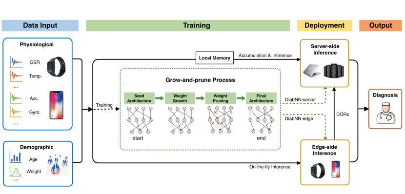
Figure 1: The schematic diagram of the proposed DiabDeep framework. DORs refer to disease-onset records. GSR, Temp., Acc., and Gyro. refer to Galvanic skin response, skin temperature, accelerometer data, and gyroscope data, respectively.

2.2 Efficient neural networks

Efficient NN design is a vibrant field. We discuss two approaches next.

Compact model architecture: One stream of research exploits the design of efficient building blocks for NN redundancy removal. For example, MobileNetV2 stacks inverted residual building blocks to effectively shrink its model size and reduce its FLOPs [17]. Ma et al. use channel shuffle operation and depth-wise convolution to deliver model compactness [18]. Wu et al. propose ShiftNet based on shift-based modules, as opposed to spatial convolution layers, to achieve substantial computation and storage cost reduction [19]. Besides, automated compact architecture design also provides a promising solution [20, 21]. Dai et al. develop efficient performance predictors to speed up the search process for efficient NNs [22]. Compared to MobileNetV2 on the ImageNet dataset, the generated ChamNets achieve up to 8.5% absolute top-1 accuracy improvement while reducing inference latency substantially.

Network compression: Compression techniques [23, 10] have emerged as another popular direction for NN redundancy removal. The pruning methodology was initially demonstrated to be effective on large CNNs by reducing the number of parameters in AlexNet by 9$\times$ and VGG by 13$\times$ for the well-known ImageNet dataset, without any accuracy loss [23]. Follow-up works have also successfully shown its effectiveness on recurrent NNs such as the LSTM [24, 25, 26]. Network growth is a complementary method to pruning that enables a sparser, yet more accurate, model before pruning starts [10, 27]. A grow-and-prune synthesis paradigm typically reduces the number of parameters in CNNs [10, 28] and LSTMs [29] by another 2$\times$, and increases the classification accuracy [10]. It enables NN based inference even on Internet-of-Things (IoT) sensors [28]. The model can be further compressed through low-bit quantization. For example, Zhu et al. show that a ternary representation of the weights instead of full-precision (32-bit) in ResNet-56 can significantly reduce memory cost while incurring only a minor accuracy loss [30]. The quantized models offer additional speedup potential for current NN accelerators [31].

Knowledge distillation: Knowledge distillation allows a compact student network to distill information (or ’dark knowledge’) from a more accurate, but computationally intensive, teacher network (or group of teacher networks) by mimicking the prediction distribution, given the same data inputs. The idea was first introduced by Hinton et al. [32]. Since then, knowledge distillation has been effectively used to discover efficient networks. Romero et al. proposed FitNets that distill knowledge from the teacher’s hint layers to teach compact students [33]. Passalis et al. enhanced the knowledge distillation process by introducing a concept called feature space probability distribution loss [34]. Yim et al. proposed fast minimization techniques based on intermediate feature maps that can also support transfer learning [35].

3 Methodology

In this section, we describe the proposed DiabDeep framework in detail. We first give a high-level overview of the entire framework. Then, we zoom into the DiabNN architecture used for DiabDeep inference, followed by a detailed description of gradient-based growth and magnitude-based pruning algorithms for DiabNN training.

3.1 The DiabDeep framework

We illustrate the proposed DiabDeep framework in Fig. 1. DiabDeep captures both physiological and demographic information as data input. It deploys a grow-and-prune training paradigm to deliver two inference models, i.e., DiabNN-server and DiabNN-edge, that enable inference on the server and on the edge, respectively. Finally, DiabDeep generates diagnosis as output. The details of data input, model training, and model inference are as follows:

• Data input: As mentioned earlier, DiabDeep focuses on (i) physiological signals and (ii) demographic information that are available in the daily context. Physiological signals can be captured by WMSs (e.g., from a smartphone and smartwatch) in a non-invasive, passive, and efficient manner. The list of collectible signals includes, but is not limited to, heart rate, body temperature, Galvanic skin response, and blood volume pulse. Additional signals such as eletromechanical and ambient environmental data (e.g., accelerometer, gyroscope, and humidity sensor readings) may also provide information on user habit tracking that offers diagnostic insights [7]. This list is expanding rapidly, given the speed of ongoing technological advancements in this field [17]. Demographics information (e.g., age, weight, gender, and height) also assists with disease diagnosis [7]. It can be easily captured and updated through a simple user interface on a smartwatch or smartphone. Then, both physiological and demographic data are aggregated and merged into a comprehensive data input for subsequent analysis.

• Model training: DiabDeep utilizes a grow-and-prune paradigm to train its NNs, as shown in the middle part of Fig. 1. It starts NN synthesis from a sparse seed architecture. It first allows the network to grow connections and neurons based on gradient information. Then, it prunes away insignificant connections and neurons based on magnitude information to drastically reduce model redundancy. This leads to improved accuracy and efficiency [10, 29], where the former is highly preferred on the server and the latter is critical at the edge. The training process generates two inference models, i.e., DiabNN-server and DiabNN-edge, for server and edge inference, respectively. Both models share the same DiabNN architecture, but vary in the choice of internal NN layers based on different resource constraints and design objectives, as explained later.
  

• Model inference: Due to the distinct inference environments encountered upon deployment, DiabNN-server and DiabNN-edge require different input data flows, as depicted by the separate data paths in Fig. 1. In DiabNN-server, data have to be accumulated in local memory, e.g., local phone/watch storage, before they can be transferred to the base station in a daily, weekly, or monthly manner, depending on user preference. As opposed to the accumulation-and-inference process, DiabNN-edge enables on-the-fly inference directly at the edge, e.g., a smartphone. This enables users to receive instantaneous diagnostic decisions. As mentioned earlier, it incurs a slight accuracy degradation (around 1%) due to the scarce energy and memory budgets on the edge. However, this deficit may be alleviated when DiabNN-edge jointly works with DiabNN-server. When an alarm is raised, DiabNN-edge can store the relevant data sections as disease-onset records (DORs) that can be later transferred to DiabNN-server for further analysis. In this manner, DiabNN-edge offers a substantial data storage reduction in the required edge memory by bypassing the storage of ’not-of-interest’ signal sections, while preserving the capability to make accurate inference on the server side. Such DORs can also be used as informative references when future physician intervention and checkup are needed.

We next explain our proposed DiabNN architecture in detail.

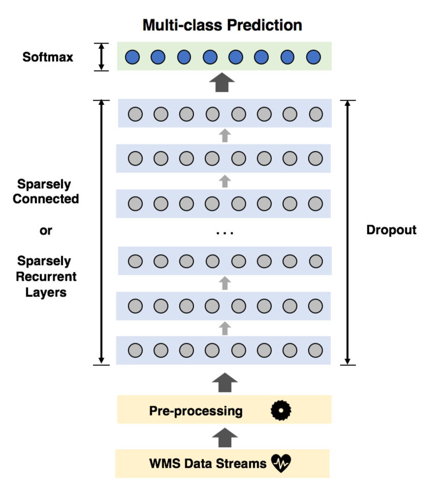
Figure 2: An illustration of the DiabNN architecture.

3.2 The DiabNN architecture

Fig. 2 shows the DiabNN architecture that distills diagnostic decisions (shown at the top) from data inputs (shown at the bottom). There are three sequential steps employed during this process: (i) data preprocessing, (ii) transformation via NN layers, and (iii) output generation using softmax. We describe these steps next.

The preprocessing stage is critical for DiabNN inference due to the following reasons:

• Data normalization: NNs typically favor normalized inputs. Normalization methods, such as min-max scaling, standardization, and L2 normalization, generally lead to accuracy and noise tolerance improvements [36, 37]. In this work, we apply min-max scaling to scale each input data stream into the [0,1] range:

  $$\textbf{x}_{normalized}=\frac{\textbf{x}-min(\textbf{x})}{max(\textbf{x})-min(\textbf{x})}$$

• Data alignment: WMS data streams may vary in their start times and sampling frequencies [38]. Therefore, we guarantee that the data streams are synchronized by checking their timestamps and applying appropriate offsets accordingly.

We use different NN layers in DiabNN for server and edge inference. DiabNN-server deploys SC layers to aim at high accuracy whereas DiabNN-edge utilizes sparsely recurrent (SR) layers to aim at extreme efficiency. All NN layers are subjected to dropout regularization, which is a widely-used approach for addressing overfitting and improving accuracy [39].

In DiabNN-server, each SC layer conducts a linear transformation (using a sparse matrix as opposed to a conventional full matrix) followed by a nonlinear activation function. As shown later, utilizing SC layers leads to more model parameters than SR layers, hence leads to an improved learning capability and higher accuracy. Consequentially, DiabNN-server achieves a 1$\%$ accuracy improvement over DiabNN-edge.

In DiabNN-edge, we base our SR layer design on the H-LSTM cell [29]. It is a variant of the conventional LSTM cell obtained through addition of hidden layers to its control gates. Fig. 3 shows the schematic diagram of an H-LSTM. Its internal computation flow is governed by the following equations:

$$\begin{split}\textbf{f}_{t}&=\sigma(\textbf{W}^{s}_{f}H^{*}([\textbf{x}_{t},\textbf{h}_{t-1}])+\textbf{b}_{f})\\ \textbf{i}_{t}&=\sigma(\textbf{W}^{s}_{i}H^{*}([\textbf{x}_{t},\textbf{h}_{t-1}])+\textbf{b}_{o})\\ \textbf{o}_{t}&=\sigma(\textbf{W}^{s}_{o}H^{*}([\textbf{x}_{t},\textbf{h}_{t-1}])+\textbf{b}_{o})\\ \textbf{g}_{t}&=tanh(\textbf{W}^{s}_{g}H^{*}([\textbf{x}_{t},\textbf{h}_{t-1}])+\textbf{b}_{g})\\ \textbf{c}_{t}&=\textbf{f}_{t}\otimes\textbf{c}_{t-1}+\textbf{i}_{t}\otimes\textbf{g}_{t}\\ \textbf{h}_{t}&=\textbf{o}_{t}\otimes tanh(\textbf{c}_{t})\\ \end{split}$$

where $\textbf{f}_{t}$, $\textbf{i}_{t}$, $\textbf{o}_{t}$, $\textbf{g}_{t}$, $\textbf{x}_{t}$, $\textbf{h}_{t}$, and $\textbf{c}_{t}$ denote the forget gate, input gate, output gate, cell update vector, input, hidden state, and cell state at step $t$, respectively; $\textbf{h}_{t-1}$ and $\textbf{c}_{t-1}$ refer to the previous hidden and cell states at step $t-1$; $H$, $\textbf{W}^{s}$, b, $\sigma$, and $\otimes$ refer to a hidden layer that performs a linear transformation followed by an activation function, sparse weight matrix, bias, $sigmoid$ function, and element-wise multiplication, respectively; ^∗ indicates zero or more $H$ layers for each NN gate. The additional hidden layers enable three advantages. First, they enhance gate control through a multi-level abstraction that can lead to accuracy gains. Second, they can be easily regularized through dropout, and thus lead to better generalization. Third, they offer a wide range of choices for internal activation functions, such as the rectified linear unit (ReLU), that can lead to faster learning [29]. Using H-LSTM based SR layers, DiabNN-edge reduces the model size by 130$\times$ and inference FLOPs by 2.2$\times$ relative to DiabNN-server.

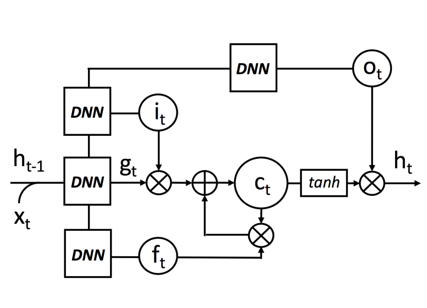
Figure 3: The schematic diagram of an H-LSTM cell. DNNs refer to deep neural network control gates.

Input: $\textbf{W}\in R^{M\times N}$: weight matrix of dimension $M\times N$, $\textbf{Msk}\in R^{M\times N}$: weight mask of dimension $M\times N$

Output: updated Msk, updated W

Denote: $\alpha$: growth ratio, $\textbf{W}.grad$: gradient of the weight matrix, $\eta$: current learning rate

Begin

Accumulate $\textbf{W}.grad$ for one training epoch

$thres$ = $(\alpha MN)^{th}$ largest element in $|\textbf{W}.grad|$

for $1\leq m\leq M$ do

       for $1\leq n\leq N$ do

             if $|W.grad_{m,n}|>thres$ then

                   $Msk_{m,n}=1$

             end if

            

       end for

      

end for

W $\leftarrow\textbf{W}+(\eta\times\textbf{W.grad}\otimes\textbf{Msk}$)

Return Msk, W

End

Algorithm 1 Gradient-based growth

Input: $\textbf{W}\in R^{M\times N}$: weight matrix of dimension $M\times N$, $\textbf{Msk}\in R^{M\times N}$: weight mask of dimension $M\times N$

Denote: $\beta$: pruning ratio

Output: updated Msk, updated W

Begin

$thres$ = $(\beta MN)^{th}$ largest element in $|\textbf{W}|$

for $1\leq m\leq M$ do

       for $1\leq n\leq N$ do

             if $|W_{m,n}|<thres$ then

                   $Msk_{m,n}=0$

             end if

            

       end for

      

end for

$\textbf{W}\leftarrow\textbf{W}\otimes\textbf{Msk}$

Return Msk, W

End

Algorithm 2 Magnitude-based pruning

3.3 Grow-and-prune training for DiabNN

We next explain the gradient-based network growth and magnitude-based network pruning algorithms in detail. Unless otherwise stated, we assume a mask-based approach for tackling sparse networks. Each weight matrix W has a corresponding binary mask matrix Msk that has the exact same size. It is used to disregard dormant connections (connections with zero-valued weights).

Algorithm 1 illustrates the connection growth process. The main objective of the weight growth phase is to locate only the most effective dormant connections to reduce the value of the loss function $L$. To do so, we first evaluate the gradient for all the dormant connections and use this information as a metric for ranking their effectiveness. During the training process, we extract the gradient of all weight matrices ($\textbf{W}.grad$) for each mini-batch of training data using the back-propagation algorithm. We repeat this process over a whole training epoch to accumulate $\textbf{W}.grad$. Then, we calculate the average gradient over the entire epoch by dividing the accumulated values by the number of training instances. We activate a dormant connection $w$ if and only if its gradient magnitude is larger than the $((1-\alpha)\times 100)^{th}$ percentile of the gradient magnitudes of its associated layer matrix. Its initial value is set to the product of its gradient value and the current learning rate. The growth ratio $\alpha$ is a hyperparameter. We typically use $0.1\leq\alpha\leq 0.3$ in our experiments. The NN growth method was first proposed in [10]. It has been shown to be very effective in enabling the network to reach a higher accuracy with far less redundancy than a fully connected model.

We show the connection pruning algorithm in Algorithm 2. During this process, we remove a connection $w$ if and only if its magnitude is smaller than the $(\beta\times 100)^{th}$ percentile of the weight magnitudes of its associated layer matrix. When pruned away, the connection’s weight value and its corresponding mask binary value are simultaneously set to zero. The pruning ratio $\beta$ is also a hyperparameter. Typically, we use $\beta\leq 0.3$ in our experiments. Connection pruning is an iterative process, where we retrain the network to recover its accuracy after each pruning iteration.

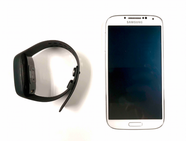
Figure 4: A photo of the Empatica E4 smartwatch (left) and the Samsung Galaxy S4 smartphone (right) used for data collection.

TABLE I: Data types collected from each participant

Data type	Source
Galvanic skin response	Smart watch
Skin temperature	Smart watch
Acceleration ($x,y,z$)	Smart watch
Inter-beat interval	Smart watch
Blood volume pulse	Smart watch
Humidity	Smart phone
Ambient illuminance	Smart phone
Ambient light color spectrum	Smart phone
Ambient temperature	Smart phone
Gravity ($x,y,z$)	Smart phone
Angular velocity ($x,y,z$)	Smart phone
Orientation ($x,y,z$)	Smart phone
Acceleration ($x,y,z$)	Smart phone
Linear acceleration ($x,y,z$)	Smart phone
Air pressure	Smart phone
Proximity	Smart phone
Wi-Fi radiation strength	Smart phone
Magnetic field strength	Smart phone
Age	Questionnaire
Gender	Questionnaire
Height	Questionnaire
Weight	Questionnaire
Relatives with diabetes	Questionnaire
Smoking	Questionnaire
Drinking	Questionnaire

4 Implementation Details

In what follows, we first describe the dataset collected from 52 participants that is used for DiabDeep evaluation. Then, we explain the implementation details of DiabDeep based on the collected dataset.

4.1 Data collection and preparation

In this study, we collected both the physiological data and demographic information from 52 participants. 27 participants were diagnosed with diabetes (14 with type-1 and 13 with type-2 diabetes) whereas the remaining 25 participants were healthy non-diabetic baselines. We collected the physiological data using a commercially available Empatica E4 smartwatch [40] and Samsung Galaxy S4 smartphone, as shown in Fig. 4. We also used a questionnaire to gather demographic information from all the participants. We summarize all the data types collected in this study in Table LABEL:tb:signal. It can be observed that the collected data cover a wide range of physiological and demographic signals that may assist with diabetes diagnosis in the daily context. The smartwatch data capture the physiological state of the target user. This information, e.g., GSR (measures the electrical activity of the skin, i.e., skin conductance) and BVP (measures cardiovascular activity, e.g., heart beat waveform and heart rate variability, etc.), has been shown to effectively capture the body status in terms of its health indicators [6]. The ambient information from the smartphone may assist with sensing of body movement and physiological signal calibration. Finally, demographic information has been previously shown to be effective for diabetes diagnosis [7]. In this work, we study whether synergies among sources of the above information collected in the daily context can support the task of pervasive diabetes diagnosis.

During data collection, we first inform all the participants about the experiment, let them sign the consent form, and ask them to fill the demographic questionnaire. Then, we place the Empatica E4 smartwatch on the wrist of participant’s non-dominant hand, and the Samsung Galaxy S4 smartphone in the participant’s pocket. The experiment lasts between 1.0 and 1.5 hours per participant during which time the smartwatch and smartphone continuously track and store the physiological signals. We use the Empatica E4 Connect portal for smartwatch data retrieval [40]. We develop an Android application to record all the smartphone sensor data streams. All the data streams contain detailed timestamps that are later used for data synchronization. The experimental procedure was approved by the Institutional Review Board of Princeton University. None of the participants reported mental, cardiac, or endocrine disorders.

We next preprocess the dataset before training the model. We first synchronize and window the WMS data streams. To avoid time correlation between adjacent data windows, we divide data into $t=15s$ windows with $s=30s$ shifts in between. The final dataset contains 5030 data instances. We use 70%, 10%, and 20% of the data as training, validation, and test sets. The training, validation, and test sets have no time overlap. We then extract the value ranges of the data streams from the training set, and then scale all three datasets based on the min-max scaling method, as explained earlier.

4.2 DiabDeep implementation

We implement the DiabDeep framework using PyTorch [41] on Nvidia GeForce GTX 1060 GPU (with 1.708GHz frequency and 6GB memory) and Tesla P100 GPU (with 1.329GHz frequency and 16GB memory). We employ CUDA 8.0 and CUDNN 5.1 libraries in our experiments. We next describe our implementation of DiabNNs based on the collected dataset.

4.2.1 DiabNN-server

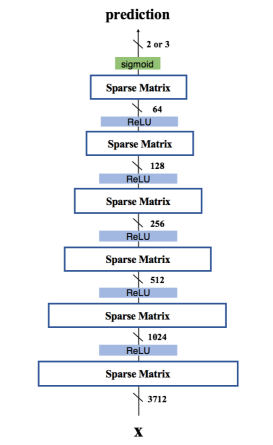
Figure 5: Architecture of DiabNN-server. x denotes the input tensor.

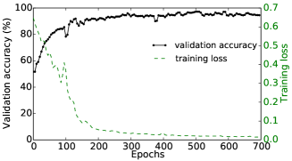
Figure 6: Training curve for DiabNN-server to distinguish among type-1 diabetic, type-2 diabetic, and healthy individuals.

We first explain the implementation details for DiabNN-server.

Data input: For each data instance, we flatten and concatenate the data within the same monitoring window from both the smartphone and smartwatch. This results in a vector of length 3705, where the flattened smartwatch window contains 2535 signal readings (from one data stream at 64Hz, three data streams at 32Hz, two data streams at 4Hz and one data stream at 1Hz), and the flattened smartphone window provides additional 1170 signal readings (from 26 data streams at 3Hz). Finally, we append the seven demographic features at its end and obtain a vector of length 3712 as the input for DiabNN-server.

Model architecture: We present the model architecture for DiabNN-server in Fig. 5. We use six sequential SC layers in DiabNN-server with widths set at 1024, 512, 256, 128, 64 and 2 (3 for three-class classification), respectively. The input dimension is the same as the input tensor dimension of 3712. We use ReLU as the nonlinear activation function for all SC layers.

Training: We use a stochastic gradient descent (SGD) optimizer with a momentum of 0.9 for this experiment. We initialize the learning rate to 0.005 and divide the learning rate by 10 when the validation accuracy does not increase in 50 consecutive epochs. We use a batch size of 256 and a dropout ratio of 0.2. For grow-and-prune training, we initialize the seed architecture with a filling rate of 20%. We grow the network for three epochs using a 0.2 growth ratio. For network pruning, we initialize the pruning ratio to 0.2. We halve the pruning ratio if the retrained model cannot restore accuracy on the validation set. We terminate the process when the ratio falls below 0.01. The training curve for DiabNN-server is presented in Fig. 6.

Figure 7: Architecture of DiabNN-edge. The denotations follow the description in Section 3.2.

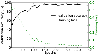
Figure 8: Training curve for DiabNN-edge to distinguish among type-1 diabetic, type-2 diabetic, and healthy individuals.

4.2.2 DiabNN-edge

We explain the implementation details for DiabNN-edge in this section.

Data input: Unlike SC layer based DiabNN-server, SR layer based DiabNN-edge acts on time series data step by step [29]. Thus, at each time step, we concatenate the temporal signal values from each data stream along with the demographic information to form an input vector of length 40 (corresponding to seven smartwatch data streams, 26 smartphone data streams, and seven demographic features, as shown in Table I). DiabNN-edge operates on four input vectors per second. When a signal reading is missing in a data stream (e.g., due to a lower sampling frequency), we use the closest previous reading in that data stream as the interpolated value.

Model architecture: We present the model architecture for DiabNN-edge in Fig. 7. DiabNN-edge contains one H-LSTM cell based SR layer that has a hidden state width of 96. Each control gate within the H-LSTM cell contains one hidden layer. We use ReLU as the nonlinear activation function.

Training: We again use an SGD optimizer with a momentum of 0.9 for this experiment. The learning rate is initialized to 0.001. We divide the learning rate by 10 when the validation accuracy does not increase in 30 consecutive epochs. We use a batch size of 64 and a dropout ratio of 0.2 for training. For grow-and-prune training, we use the same hyperparameter set as in the experiment for DiabNN-server. The training curve for DiabNN-edge is presented in Fig. 8.

TABLE II: Performance evaluation metrics

Name	Definition
Accuracy	$(TP+TN)/(TP+FP+FN+TN)$
False positive rate	$FP/(TN+FP)$
False negative rate	$FN/(TP+FN)$
F1 score	$2TP/(2TP+FP+FN)$
$TP(TN)$: diabetic (healthy) instances classified as diabetic (healthy)
$FP(FN)$: healthy (diabetic) instances classified as diabetic (healthy)

5 Evaluating DiabDeep Performance

In this section, we first analyze the performance of DiabNN-server and DiabNN-edge for two classification tasks: (i) binary classification that distinguishes between diabetic vs. healthy individuals, and (ii) three-class classification to distinguish among type-1 diabetic, type-2 diabetic, and healthy individuals. Then, we compare the performances of DiabNN-server, DiabNN-edge, and the relevant baselines.

We evaluate the performance of DiabNNs using four performance metrics, as summarized in Table II. Accuracy indicates the overall prediction capability. The false positive rate (FPR) and false negative rate (FNR) measure the DiabNN’s capability to avoid misclassifying healthy and diabetic instances, respectively. The F1 score measures the overall performance of precision and sensitivity.

5.1 DiabNN-server performance evaluation

We first analyze the performance of DiabNN-server. Table III presents the confusion matrix of DiabNN-server for the binary classification task. DiabNN-server achieves an overall accuracy of 96.3%. For the healthy instances, it achieves a very low FPR of 4.3%, demonstrating its effectiveness in avoiding false alarms. For the diabetic instances, it achieves an FNR of 3.1%, indicating its effectiveness in raising alarms when diabetes does occur. DiabNN-server achieves an F1 score of 96.5% for the binary classification task.

We present the confusion matrix of DiabNN-server for the three-class classification task in Table IV. DiabNN-server achieves an overall accuracy of 95.7%. For the healthy instances, it achieves a low FPR of 6.6%, again demonstrating its ability to avoid false alarms. It also delivers low FNRs for both type-1 and type-2 diabetic individuals of 1.6% and 2.8%, respectively (each FNR depicts the ratio of the number of false predictions for a target diabetes type divided by the total number of instances of that type). DiabNN-server achieves an F1 score of 95.7% for the three-class classification task.

Furthermore, the grow-and-prune training paradigm not only delivers high diagnostic accuracy, but also leads to model compactness as a side benefit. For binary classification, the final DiabNN-server model contains only 429.1K parameters with a sparsity level of 90.5%. For the three-class classification task, the final DiabNN-server model contains only 445.8K parameters with a sparsity level of 90.1%. The model compactness achieved in both cases can help reduce storage and energy consumption on the server.

5.2 DiabNN-edge performance evaluation

We next analyze the performance of DiabNN-edge. We present the confusion matrix of DiabNN-edge for the binary classification task in Table V. DiabNN-edge achieves an overall accuracy of 95.3%. For the healthy case, it also achieves a very low FPR of 3.7%. For diabetic instances, it achieves an FNR of 5.6%. This shows that DiabNN-edge can also effectively raise disease alarms on the edge. DiabNN-edge achieves an F1 score of 95.4% for the binary classification task.

TABLE III: DiabNN-server confusion matrix for binary classification

		prediction
		diabetic	healthy	total
label	diabetic	504	16	520
	healthy	21	465	486
	total	525	481	1006

TABLE IV: DiabNN-server confusion matrix for three-class classification

		prediction
		type-1	type-2	healthy	total
label	type-1	303	1	4	308
	type-2	5	206	1	212
	healthy	22	10	454	486
	total	330	217	459	1006

TABLE V: DiabNN-edge confusion matrix for binary classification

		prediction
		diabetic	healthy	total
label	diabetic	491	29	520
	healthy	18	468	486
	total	509	497	1006

TABLE VI: DiabNN-edge confusion matrix for three-class classification

		prediction
		type-1	type-2	healthy	total
label	type-1	288	4	16	308
	type-2	7	200	5	212
	healthy	12	10	464	486
	total	307	214	485	1006

TABLE VII: Performance comparison between DiabNN-server and DiabNN-edge

Performance matrices	DiabNN-server	DiabNN-edge
Accuracy	96.3%	95.3%
FPR	4.3%	3.7%
FNR	3.1%	5.6%
F1	96.5%	95.4%
FLOPs	858.2K	392.8K
#Parameters	429.1K	3.3K

We also evaluate DiabNN-edge for the three-class classification task and present the confusion matrix in Table VI. DiabNN-edge achieves an overall accuracy of 94.6%. For the healthy case, it achieves an FPR of 4.5%. It achieves FNRs of 6.5% and 5.7% for the type-1 and type-2 diabetic instances, respectively. DiabNN-server achieves an F1 score of 94.4% for the three-class classification task.

DiabNN-edge delivers extreme model compactness. For binary classification, the final DiabNN-edge model contains a sparsity level of 96.3%, yielding a model with only 3.3K parameters. For the three-class classification task, the final DiabNN-edge model contains a sparsity level of 95.9%, yielding a model with only 3.7K parameters. This greatly assists with inference on the edge that typically suffers from very limited resource budgets.

5.3 Results analysis

As mentioned earlier, DiabNN-edge and DiabNN-server offer several performance tradeoffs over diagnostic accuracy, storage cost, and run-time efficiency. This provides flexible design choices that can accommodate varying design objectives related to model deployment. To illustrate their differences, we compare these two models for the binary classification task in Table LABEL:tb:edge_server. We observe that DiabNN-server achieves a higher accuracy, a higher F1 score, and a lower FNR. DiabNN-edge, on the other hand, caters to edge-side inference by enabling:

• A smaller model size: The edge model contains $130\times$ fewer parameters, leading to a substantial memory reduction.

• Less computation: It requires 2.2$\times$ fewer FLOPs per inference, enabling a more efficient, hence more frequent, monitoring capability on the edge.

• A lower FPR: It reduces the FPR by 0.6$\%$. This enables fewer false alarms and hence an improved usability for the system in a daily usage scenario.

We also analyze the performance tradeoffs under changing model complexity and present the results in Fig. 9. It can be observed that an increase in computational complexity can lead to performance improvements, in general. However, such benefits gradually degrade as the computation complexity continues to increase.

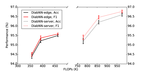
(a) Change of accuracy and F1 score against model complexity.

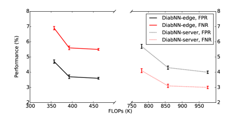
(b) Change of FPR and FNR against model complexity.

Figure 9: Performance tradeoffs against model complexity based on five runs per data point with different random seeds. Error bars denote standard deviations.

TABLE VIII: Inference model comparison between DiabNNs and conventional methods

Model	Accuracy	#Parameters	Feature extraction	Classification	Total FLOPs
			FLOPs	FLOPs
SVM-linear	86.3%	699K	0.49M	1.39M	1.88M
SVM-RBF	92.1%	822K	0.49M	1.65M	2.14M
k-NN	93.5%	1.5M	0.49M	3.0M	3.49M
Random forest	92.6%	8K	0.49M	4K+	0.49M∗
Linear ridge	81.3%	0.8K	0.49M	1.6K	0.49M
DiabNN-server	96.3%	429K	-	0.86M	0.86M
DiabNN-edge	95.3%	3.3K	-	0.39M	0.39M
$+$: Number of comparison operations.
$*$: Calculation excluding the comparison operation cost.

TABLE IX: Performance comparison between DiabDeep and related work

	Data sources	Model	Accuracy
Swapna et al.[16]	ECG sensor	Conv-LSTM	95.1%
Swapna et al.[16]	ECG sensor	CNN	93.6%
Ballinger et al. [15]	Watch + demographics	LSTM	84.5%
Yin et al. [7]	Watch + demographics	Ensemble	77.6%
This work (DiabNN-server)	Watch + phone + demographics	Stacked SC layers	96.3%
This work (DiabNN-edge)	Watch + phone + demographics	H-LSTM SR layer	95.3%

We next compare DiabNNs with widely-used learning methods, including SVMs with linear and RBF kernels, k-NN, random forest, and linear ridge classifiers. For all the methods, we use the same train/validation/test split and the same binary classification task for a fair comparison. In line with the studies in [42] and [43], we extract the signal mean, variance, Fourier transform coefficients, and the third-order Daubechies wavelet transform approximation and detail coefficients on Daubechies D2, D4, D8, and D24 filters from each monitoring window, resulting in a feature vector of length 304 per data instance. We train all our non-NN baselines using the Python-based Scikit learn libraries [44]. We compare the performance of all the inference models in Table LABEL:tb:energy_compare. In addition to classification accuracy, we also compute the necessary FLOPs per inference involved in both feature extraction and classification stages. We can see that DiabNN-server achieves the highest accuracy among all the models. With a higher accuracy than all the non-NN baselines, DiabNN-edge achieves the smallest model size (up to 454.5$\times$ reduction) and least FLOPs per inference (up to 8.9$\times$ reduction). Note that the feature extraction stage accounts for 491K FLOPs even before the classification stage starts executing. This is already 1.3$\times$ the total inference cost of DiabNN-edge.

Finally, we compare DiabDeep with relevant work from the literature in Table LABEL:tb:lit. We also focus on the same binary classification task that is the focus of these studies. DiabDeep achieves the highest accuracy relative to the baselines due to its two major advantages. First, it relies on a more comprehensive set of WMSs. This captures a wider spectrum of user signals in the daily context for diagnostic decisions. Moreover, it utilizes a grow-and-prune training paradigm that learns both the connections and weights in DiabNNs. This enables a more effective SGD in both the model architecture space and parameter space.

6 Discussions & Future work

In this section, we discuss the inspirations we took from human brains to train DiabNNs as well as the future directions enabled by DiabDeep.

Our brains continually remold the synaptic connections as we acquire new knowledge. These changes happen every second throughout our lifetimes. It has even been shown that most knowledge acquisition and information learning processes in our brains result from such a synaptic rewiring, also referred to as neuroplasticity [45]. This is very different from most current NNs that have a fixed architecture. To mimic the learning mechanism of human brains, we utilize gradient-based growth and magnitude-based pruning to train accurate, yet very compact, DiabNNs for DiabDeep. The grow-and-prune synthesis paradigm allows DiabNNs to easily adjust their synaptic connections to the diabetes diagnosis task.

DiabDeep opens up the potential for future WMS-based disease diagnosis studies, given that more than 69,000 diseases exist [7]. We hope that this work will encourage clinics/hospitals/researchers to start collecting WMS data from individuals across more challenging diagnostic tasks, e.g., for long-term cancer prediction. Bypassing the feature extraction stage with efficient NNs enables easy scalability of the proposed approach across other disease domains. The grow-and-prune synthesis paradigm may even support continuous disease trend forecasting capability, given its continuous learning capability [27]. As more data become available and analyzed with the proposed methodology, its effectiveness as a scalable approach for future pervasive diagnosis and medication level determination will continue to improve.

7 Conclusions

In this work, we proposed a framework called DiabDeep that combines off-the-shelf WMSs with efficient DiabNNs for continuous and pervasive diabetes diagnosis on both the server and the edge. On the resource-rich server, we deployed stacked SC layers to focus on high accuracy. On the resource-scarce edge, we used an H-LSTM based SR layer to reduce computation and storage costs with only a minor accuracy loss. We trained DiabNNs by leveraging gradient-based growth and magnitude-based pruning algorithms. This enables DiabNNs to learn both weights and connections during training. We evaluated DiabDeep based on data collected from 52 participants. Our system achieves a 96.3% (95.3%) accuracy in classifying diabetics against healthy individuals on the server (edge), and a 95.7% (94.6%) accuracy in distinguishing among type-1 diabetic, type-2 diabetic, and healthy individuals. Against conventional baselines, such as SVMs with linear and RBF kernels, k-NN, random forest, and linear ridge classifiers, DiabNN-edge reduces model size (FLOPs) by up to 454.5$\times$ (8.9$\times$) while improving accuracy. Thus, we have demonstrated that DiabDeep can be employed in a pervasive fashion, while offering high efficiency and accuracy.

References

- [1] B. Zhou, Y. Lu, K. Hajifathalian, J. Bentham, M. Di Cesare, G. Danaei, H. Bixby, M. Cowan, M. Ali, C. Taddei, W. Lo, B. Reis-Santos, G. Stevens, L. Riley, J. Miranda, P. Bjerregaard, J. Rivera, H. Fouad, G. Ma, J. Mbanya, S. McGarvey, V. Mohan, A. Onat, A. Pilav, A. Ramachandran, H. Ben Romdhane, C. Paciorek, J. Bennett, M. Ezzati, Z. Abdeen, K. Kadir, N. Abu-Rmeileh, B. Acosta-Cazares, R. Adams, W. Aekplakorn, C. Aguilar-Salinas, C. Agyemang, A. Ahmadvand, A. Al-Othman, A. Alkerwi, P. Amouyel, A. Amuzu, L. Bo Andersen, S. Anderssen, R. Anjana, H. Aounallah-Skhiri, T. Aris, N. Arlappa, J. Hata, and T. Ninomiya, “Worldwide trends in diabetes since 1980: A pooled analysis of 751 population-based studies with 4.4 million participants,” The Lancet, vol. 387, no. 10027, pp. 1513–1530, 2016.
- [2] W. Yang, T. Dall, K. Beronijia, J. Lin, A. Semilla, R. Chakrabarti, and P. Hogan, “Economic costs of diabetes in the U.S. in 2017,” Diabetes Care, vol. 41, no. 5, pp. 917–928, 2018.
- [3] “Global report on diabetes,” 2016. [Online]. Available: https://apps.who.int.
- [4] W. R. Rowley, C. Bezold, Y. Arikan, E. Byrne, and S. Krohe, “Diabetes 2030: Insights from yesterday, today, and future trends,” Population Health Management, vol. 20, no. 1, pp. 6–12, 2017.
- [5] A. Facchinetti, “Continuous glucose monitoring sensors: Past, present and future algorithmic challenges,” Sensors, vol. 16, no. 12, pp. 2093–2104, 2016.
- [6] H. Yin, A. O. Akmandor, A. Mosenia, and N. K. Jha, “Smart healthcare,” Foundations and Trends in Electronic Design Automation, vol. 12, no. 4, pp. 401–466, 2018.
- [7] H. Yin and N. K. Jha, “A health decision support system for disease diagnosis based on wearable medical sensors and machine learning ensembles,” IEEE Trans. Multi-Scale Computing Systems, vol. 3, no. 4, pp. 228–241, 2017.
- [8] H. Zhang, P.-H. Chen, and P. Ramadge, “Transfer learning on fMRI datasets,” in Proc. Int. Conf. Artificial Intelligence and Statistics, 2018.
- [9] H. Quan, V. Sundararajan, P. Halfon, A. Fong, B. Burnand, J.-C. Luthi, L. D. Saunders, C. A. Beck, T. E. Feasby, and W. A. Ghali, “Coding algorithms for defining comorbidities in ICD-9-CM and ICD-10 administrative data,” Medical Care, pp. 1130–1139, 2005.
- [10] X. Dai, H. Yin, and N. K. Jha, “NeST: A neural network synthesis tool based on a grow-and-prune paradigm,” IEEE Trans. on Computers, 2019.
- [11] T. Zheng, W. Xie, L. Xu, X. He, Y. Zhang, M. You, G. Yang, and Y. Chen, “A machine learning-based framework to identify type 2 diabetes through electronic health records,” Int. J. Medical Informatics, vol. 97, pp. 120–127, 2017.
- [12] I. Kavakiotis, O. Tsave, A. Salifoglou, N. Maglaveras, I. Vlahavas, and I. Chouvarda, “Machine learning and data mining methods in diabetes research,” J. Computational and Structural Biotechnology, vol. 15, pp. 104–116, 2017.
- [13] V. Gulshan, L. Peng, M. Coram, M. C. Stumpe, D. Wu, A. Narayanaswamy, S. Venugopalan, K. Widner, T. Madams, J. Cuadros, R. Kim, R. Raman, P. Nelson, J. Mega, and D. Webster, “Development and validation of a deep learning algorithm for detection of diabetic retinopathy in retinal fundus photographs,” J. American Medical Association, vol. 316, no. 22, pp. 2402–2410, 2016.
- [14] R. Ajjan, D. Slattery, and E. Wright, “Continuous glucose monitoring: A brief review for primary care practitioners,” Advances in Therapy, vol. 36, no. 3, pp. 579–596, 2019.
- [15] B. Ballinger, J. Hsieh, A. Singh, N. Sohoni, J. Wang, G. H. Tison, G. M. Marcus, J. M. Sanchez, C. Maguire, J. E. Olgin, and M. J. Pletcher, “DeepHeart: Semi-supervised sequence learning for cardiovascular risk prediction,” in Proc. AAAI Conf. Artificial Intelligence., 2018, pp. 2079–2086.
- [16] G. Swapna, S. Kp, and R. Vinayakumar, “Automated detection of diabetes using CNN and CNN-LSTM network and heart rate signals,” Procedia Computer Science, vol. 132, pp. 1253–1262, 2018.
- [17] M. Sandler, A. Howard, M. Zhu, A. Zhmoginov, and L.-C. Chen, “Inverted residuals and linear bottlenecks: Mobile networks for classification, detection and segmentation,” arXiv preprint arXiv:1801.04381, 2018.
- [18] N. Ma, X. Zhang, H.-T. Zheng, and J. Sun, “ShuffleNet V2: Practical guidelines for efficient CNN architecture design,” arXiv preprint arXiv:1807.11164, 2018.
- [19] B. Wu, A. Wan, X. Yue, P. Jin, S. Zhao, N. Golmant, A. Gholaminejad, J. Gonzalez, and K. Keutzer, “Shift: A zero FLOP, zero parameter alternative to spatial convolutions,” in Proc. IEEE Conf. Computer Vision and Pattern Recognition, 2018, pp. 9127–9135.
- [20] B. Wu, X. Dai, P. Zhang, Y. Wang, F. Sun, Y. Wu, Y. Tian, P. Vajda, Y. Jia, and K. Keutzer, “FBNet: Hardware-aware efficient ConvNet design via differentiable neural architecture search,” in Proc. IEEE Conf. Computer Vision and Pattern Recognition, 2019.
- [21] Y. Zhou and G. Diamos, “Neural architect: A multi-objective neural architecture search with performance prediction,” in Proc. Conf. SysML, 2018.
- [22] X. Dai, P. Zhang, B. Wu, H. Yin, F. Sun, Y. Wang, M. Dukhan, Y. Hu, Y. Wu, Y. Jia, P. Vajda, M. Uyttendaele, and N. K. Jha, “ChamNet: Towards efficient network design through platform-aware model adaptation,” in Proc. IEEE Conf. Computer Vision and Pattern Recognition, 2019, pp. 11 398–11 407.
- [23] S. Han, J. Pool, J. Tran, and W. J. Dally, “Learning both weights and connections for efficient neural network,” in Proc. Advances in Neural Information Processing Systems, 2015, pp. 1135–1143.
- [24] S. Han, J. Kang, H. Mao, Y. Hu, X. Li, Y. Li, D. Xie, H. Luo, S. Yao, Y. Wang, H. Yang, and W. J. Dally, “ESE: Efficient speech recognition engine with sparse LSTM on FPGA,” in Proc. ACM/SIGDA Int. Symp. Field-Programmable Gate Arrays, 2017, pp. 75–84.
- [25] W. Wen, Y. He, S. Rajbhandari, W. Wang, F. Liu, B. Hu, Y. Chen, and H. Li, “Learning intrinsic sparse structures within long short-term memory,” arXiv preprint arXiv:1709.05027, 2017.
- [26] S. Narang, E. Elsen, G. Diamos, and S. Sengupta, “Exploring sparsity in recurrent neural networks,” arXiv preprint arXiv:1704.05119, 2017.
- [27] X. Dai, H. Yin, and N. K. Jha, “Incremental learning using a grow-and-prune paradigm with efficient neural networks,” arXiv preprint arXiv:1905.10952, 2019.
- [28] S. Hassantabar, Z. Wang, and N. K. Jha, “SCANN: Synthesis of compact and accurate neural networks,” arXiv preprint arXiv:1904.09090, 2019.
- [29] X. Dai, H. Yin, and N. K. Jha, “Grow and prune compact, fast, and accurate LSTMs,” arXiv preprint arXiv:1805.11797, 2018.
- [30] C. Zhu, S. Han, H. Mao, and W. J. Dally, “Trained ternary quantization,” arXiv preprint arXiv:1612.01064, 2016.
- [31] H. Jia, Y. Tang, H. Valavi, J. Zhang, and N. Verma, “A microprocessor implemented in 65nm CMOS with configurable and bit-scalable accelerator for programmable in-memory computing,” arXiv preprint arXiv:1811.04047, 2018.
- [32] G. Hinton, O. Vinyals, and J. Dean, “Distilling the knowledge in a neural network,” arXiv preprint arXiv:1503.02531, 2015.
- [33] A. Romero, N. Ballas, S. E. Kahou, A. Chassang, C. Gatta, and Y. Bengio, “FitNets: Hints for thin deep nets,” arXiv preprint arXiv:1412.6550, 2014.
- [34] N. Passalis and A. Tefas, “Learning deep representations with probabilistic knowledge transfer,” in Proc. European Conf. Computer Vision, 2018, pp. 268–284.
- [35] J. Yim, D. Joo, J. Bae, and J. Kim, “A gift from knowledge distillation: Fast optimization, network minimization and transfer learning,” in Proc. IEEE Conf. Computer Vision and Pattern Recognition, 2017, pp. 4133–4141.
- [36] A. Krizhevsky, I. Sutskever, and G. E. Hinton, “ImageNet classification with deep convolutional neural networks,” in Proc. Advances in Neural Information Processing Systems, 2012, pp. 1097–1105.
- [37] Z. He, T. Zhang, and R. B. Lee, “Verideep: Verifying integrity of deep neural networks through sensitive-sample fingerprinting,” in Proc. IEEE Conf. Computer Vision and Pattern Recognition, 2019.
- [38] H. Yin, Z. Wang, and N. K. Jha, “A hierarchical inference model for Internet-of-Things,” IEEE Trans. Multi-Scale Computing Systems, vol. 4, pp. 260–271, 2018.
- [39] A. Krizhevsky, I. Sutskever, and G. E. Hinton, “ImageNet classification with deep convolutional neural networks,” in Proc. Advances in Neural Information Processing Systems, 2012, pp. 1097–1105.
- [40] “Empatica E4 connect portal,” 2019. [Online]. Available: https://www.empatica.com/connect.
- [41] A. Paszke, S. Gross, S. Chintala, G. Chanan, E. Yang, Z. DeVito, Z. Lin, A. Desmaison, L. Antiga, and A. Lerer, “Automatic differentiation in PyTorch,” NIPS Workshop Autodiff, 2017.
- [42] S. Mahmoodabadi, A. Ahmadian, and M. Abolhasani, “ECG feature extraction using Daubechies wavelets,” in Proc. Int. Conf. Visualization, Imaging and Image Processing, 2005, pp. 343–348.
- [43] A. Gupta, R. Agrawal, and B. Kaur, “Performance enhancement of mental task classification using EEG signal: A study of multivariate feature selection methods,” Soft Computing, vol. 19, no. 10, pp. 2799–2812, 2015.
- [44] F. Pedregosa, G. Varoquaux, A. Gramfort, V. Michel, B. Thirion, O. Grisel, M. Blondel, P. Prettenhofer, R. Weiss, V. Dubourg, J. Vanderplas, A. Passos, D. Cournapeau, M. Brucher, M. Perrot, and E. Duchesnay, “Scikit-learn: Machine learning in Python,” J. Machine Learning Research, vol. 12, pp. 2825–2830, Oct. 2011.
- [45] S. Grossberg, “Nonlinear neural networks: Principles, mechanisms, and architectures,” Neural Networks, vol. 1, no. 1, pp. 17–61, 1988.