The Detection of Distributional Discrepancy for Text Generation
Abstract
The text generated by neural language models is not as good as the real text. This means that their distributions are different. Generative Adversarial Nets (GAN) are used to alleviate it. However, some researchers argue that GAN variants do not work at all. When both sample quality (such as Bleu) and sample diversity (such as self-Bleu) are taken into account, the GAN variants even are worse than a well-adjusted language model. But, Bleu and self-Bleu can not precisely measure this distributional discrepancy. In fact, how to measure the distributional discrepancy between real text and generated text is still an open problem. In this paper, we theoretically propose two metric functions to measure the distributional difference between real text and generated text. Besides that, a method is put forward to estimate them. First, we evaluate language model with these two functions and find the difference is huge. Then, we try several methods to use the detected discrepancy signal to improve the generator. However the difference becomes even bigger than before. Experimenting on two existing language GANs, the distributional discrepancy between real text and generated text increases with more adversarial learning rounds. It demonstrates both of these language GANs fail.
1 Introduction
Text generation by neural language models (LM), such as LSTM (Hochreiter & Schmidhuber, 1997) have given rise to much progress and are now used to dialogue generation (Li et al., 2017), machine translation (Wu et al., 2016) and image caption (Xu et al., 2015). However, the generated sentences are still low quality as regards semantics and global coherence and not even perfect grammatically speaking (Caccia et al., 2019).
These issues give rise to large discrepancy between generated text and real text. One underlying reason is the architecture and number of parameters of the LM itself (Radford et al., 2019; Santoro et al., 2018). Many researchers attribute this to exposure bias (Bengio et al., 2015) because the LM is trained with a maximum likelihood estimate (MLE) and predicts the next word conditioned on words from the ground-truth during training. Yet it only conditions on words generated by itself during reference.
Statistically, this discrepancy means the two distributional functions of real texts and generated texts is different. Reducing this distributional difference may be a practicable way to improve text generation.
Some researchers try to reduce this difference with GAN (Goodfellow et al., 2014). They use a discriminator to detect the discrepancy between real samples and generated samples, and feed the signal back to upgrade the generator (a LM). In order to solve the non-differential issue that arises by the need to handle discrete tokens, reinforcement learning (RL) (Williams, 1992) is adapted by SeqGAN (Yu et al., 2017), RankGAN (Lin et al., 2017), and LeakGAN (Guo et al., 2018). The Gumble-Softmax is also introduced by GSGAN (Jang et al., 2017) and RelGAN (Nie et al., 2019) to solve this issue. These language GANs pre-train both the generator () and the discriminator () before adversarial learning111An exception is RelGAN which does not need not to pre-train .. During adversarial learning, for each round, the is trained several epochs and then, the is trained tens of epochs. Learning stops when the model converges. Furthermore, considering the generated texts’ quality and diversity simultaneously (Shi et al., 2018), MaskGAN (Fedus et al., 2018), DpGAN (Xu et al., 2018), FMGAN (Chen et al., 2018) and RelGAN (Nie et al., 2019) are proposed. They evaluate the generated text with Bleu and self-Bleu (Zhu et al., 2018) or LM score and reverse LM score (Cífka et al., 2018), and claim these GANs improve the performance of the generator.
However recently questions have been raised over these claims. Semeniuta et al. (2018) and Caccia et al. (2019) showed that via more precise experiments and evaluation, these considered GAN variants are out-performed by a well-adjusted language model . d’Autume et al. (2019) trained language GANs from scratch, nevertheless, they only achieve ”comparable” performance against the LM. He et al. (2019) quantifies the exposure bias and concludes it is either 3 percent lower in performance or indistinguishable.
All the aforementioned methods treat GAN as a black box for evaluation. For those language GANs, there are several critical issues which have not been resolved, such as whether the detects the discrepancy, whether the detected discrepancy is severe, and whether the signals from can improve the generator. In this paper, we try to solve these problems via investigating GAN in both pre-training and the adversarial learning process. Theoretically analysing the signal from , we obtain two metric functions to measure the distributional difference. With these two functions, we first measure the difference between the real text and the generated text by a MLE-trained language model (pre-train). Second, we try some methods to update the generator with a feedback signal from , then, we use these metric functions to evaluate the updated generator. Finally, we analysis the existing language GANs during adversarial learning with these two functions. All the code and data can be find https://github.com/.
Our contributions are as follows:
-
•
We propose two metric functions to measure the distributional difference between real text and generated text. In addition, a method is put forward to estimate these.
-
•
Evaluated using these two functions, a number of experiments show there is an obvious discrepancy between the real text and the generated text even when it is generated by a well-adjusted language model.
-
•
Although this discrepancy could be detected by , the feedback signal from can not improve using existing methods.
-
•
Experimenting on two existing language GANs, SeqGAN and RelGAN, the distributional discrepancy between real text and generated text increases with more adversarial learning rounds. This demonstrates that both of these language GANs fail.
2 Method
In GAN, the generator implicitly defines a probability distribution to mimic the real data distribution .
| (1) |
We define to detect the discrepancy between and . We optimize as follows:
| (2) |
Assuming is the optimal solution for a given , according to (Goodfellow et al., 2014), it will be,
| (3) |
We obtain two metric functions to measure this discrepancy. This sentence should be put the next paragraph.
| (4) |
With this, the integration of the density function can be transformed into an equation for a statistic. Based on this, we can obtain a way which, described below, to compute the precise discrepancy.
2.1 Approximate Discrepancy
Let,
| (5) |
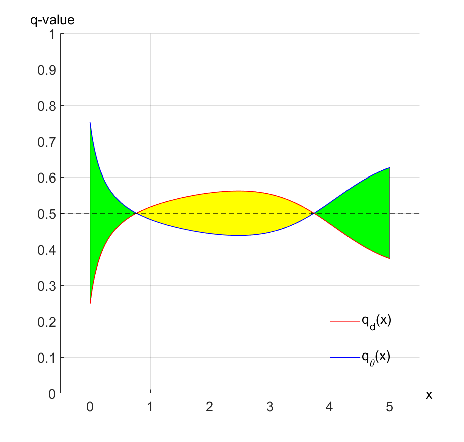
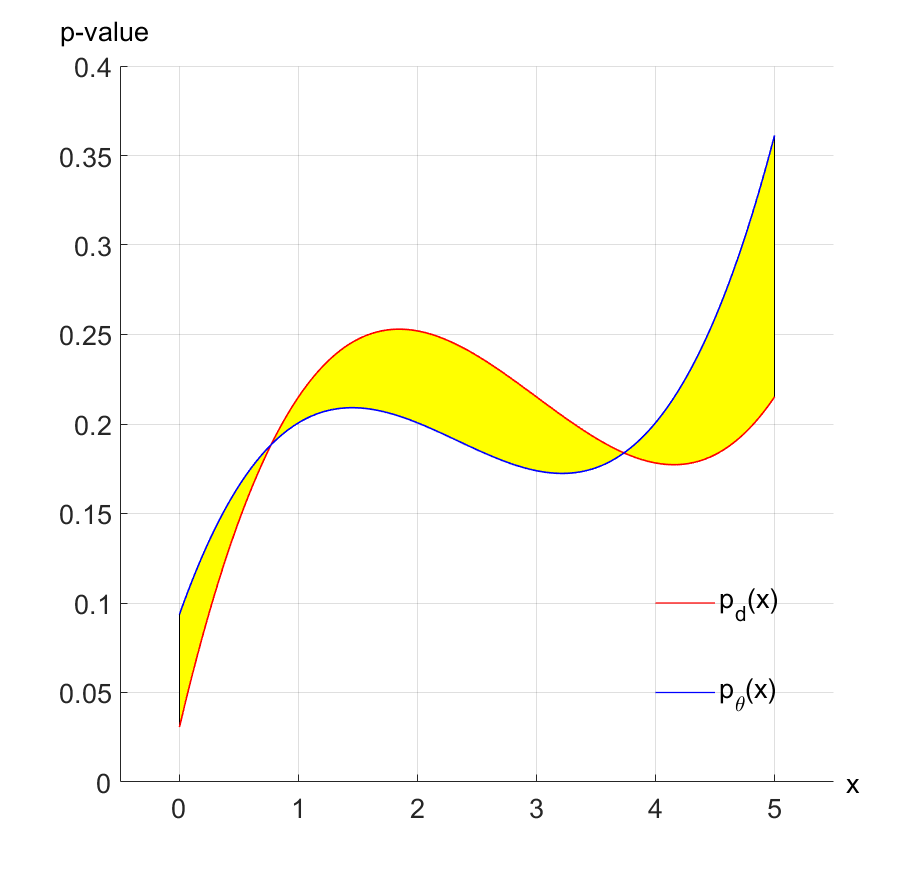
So, comes from real data, comes from generated data, . With equation 5, we can get a constraint and an approximate measure of distributional function. Figure 1(a) illustrates the relationship between and .
Let,
| (6) |
These are two equations for these two statistics which are the expectation of the ’s predictions on real text and on generated text respectively. From the above equation, it is easy to obtain the following equation:
| (7) |
It gives a constraint for converging to . We should take this constraint into account when estimating the ideal function . From equation 3, the process of optimizing the discriminator is to make big and make small. So, we can estimate the distributional discrepancy according to the following function.
Intuitively, using and , we get a metric function to measure the discrepancy between and ,
| (8) |
We call this approximate discrepancy. It is the difference in the average score that a well-trained discriminator (denoted as ) makes in the predictions on real samples compared to generated samples. It reflects the discrepancy between these two sets to some degree. From equation 5, 6 and 8, we get equation 9,
| (9) |
Figure 1 (a) illustrates the discrepancy between two distributional functions and . Both of them are systematic to the line of . But it is not a complete measure because there is not only a positive part but also a negative part. A complete metric function is given in the next section.
2.2 Absolute Discrepancy
In order to precisely measure the discrepancy, we define ,
| (10) |
The range of this function is . The bigger its value is, the larger the discrepancy. When its value is zero, it means , namely there is no discrepancy. Fortunately, this function can be estimated by using a statistic method which is described by the following equation. The proof is shown in appendix A.
| (11) |
2.3 Using to improve
Given an instance generated by , if is larger, it means the possibility of in real data is larger. For an instance , there will be according to equation 3. So, we should update to make the probability density increase. It may improve the performance of . Based on this, we can select out some generated instances by the value of to update the generator. In fact, we find it helpful to use the faked samples whose score are higher assigned by . Experiment 4.3 shows the results.
3 Implementation Procedure
The optimal function is an ideal function which can only be statistically estimated by an approximated function. We can design a function and sample from real data and generated data, then train according to equation 2. When it convergences, we get . is the approximated function of . The degree of approximation is mainly determined by three factors: the structure and the number of the parameters number of , the volume of training data, and the settings of hyper-parameters.
Based on the above analysis, we get two metric functions to measure the distributional discrepancy between dataset and . The specific implementation procedure is as follows:
Step 1: Design a discriminator .
Step 2: The sets and are respectively each divided into a training set and , a validation set and , and a test set and . The partition should be as equal an amount of instances as possible for classification training.
Step3: is optimized with and according to the equation 2. Validated with and , we can judge whether convergences or not and then get .
Step4: According to equation 8 and 11, with two test datasets, we can estimate the discrepancy of two distributional density functions between dataset and . denotes the absolute discrepancy and denotes the approximate discrepancy respectively.
Generally speaking, there should be . Because can not be obtained, it is hard to get the degree of the approximation to . Many research results have shown that the discriminators with deep neural networks are very powerful, and can even exceed human performance on some tasks such as image classification (He et al., 2016) and text classification (Kim, 2014). So, if the with CNN and attention mechanism is well trained, will be a meaningful approximation of . Therefore, we can obtain the meaningful approximation of and via .
4 Experiment
We select SeqGAN and RelGAN as representative models for our experiment and the benchmark datasets are also the same as used by these models previously. Then, we show that the well trained discriminator can measure the discrepancy between the real and generated texts, and then point out the existing GAN-based methods does not work. Finally, a third party discriminator is used to evaluate the performance of adversarial learning with incremental training iterations.
4.1 Datasets and Model Settings
Both SeqGAN and RelGAN are experimented on using relative short sentences (COCO image caption) 222http://cocodataset.org/ and a long sentences dataset (EMNLP2017 WMT news) 333http://www.statmt.org/wmt17/. For the former dataset, the sentences average length is about 11 words. There are in total 4,682 word types and the longest sentence consists of 37 words. Both the training and test data contain 10,000 sentences. For the latter dataset, the average length of sentences is about 20 words. There are in total 5,255 word types and the longest sentence consists of 51 words. All training data, about 280 thousand sentences, is used and there are 10,000 sentences in the test data. According to section 3, each test data is divided into two parts. Half is the validation set and the remaining half is the test set. We always generate the same amount of sentences to compare with the two test datasets respectively.
For these two models, all hyper-parameters including word embedding size, learning rate and dropout are set the same as in their original papers. For RelGAN, the standard GAN loss function (the non-saturating version) is adapted because the relative standard loss which is used in (Nie et al., 2019) does not meet the constraints of equation 7. But, when measuring RelGAN’s discrepancy during the adversarial stage, it own loss function is still relative standard loss. A critical hyper-parameters, temperature, is set to 100 which is the best result in their paper. During the process of training , we always train 10,000 epochs and observe performance on the validation dataset.
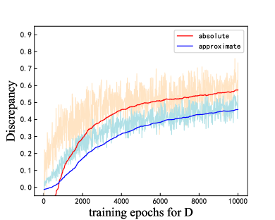
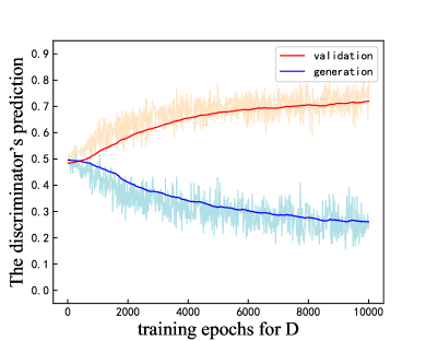
4.2 The distributional difference in Pre-training
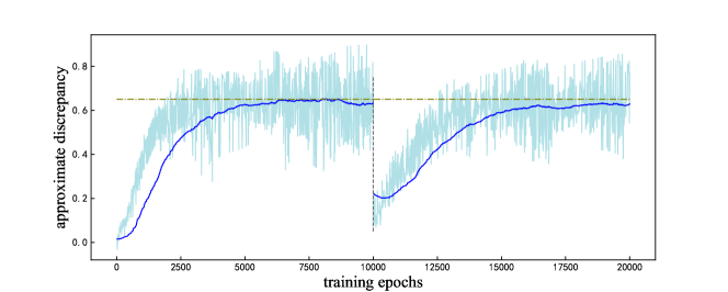
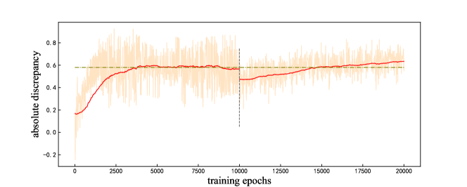
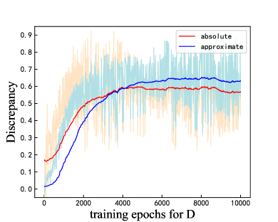
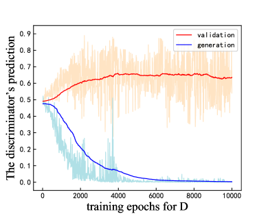
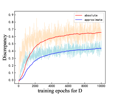
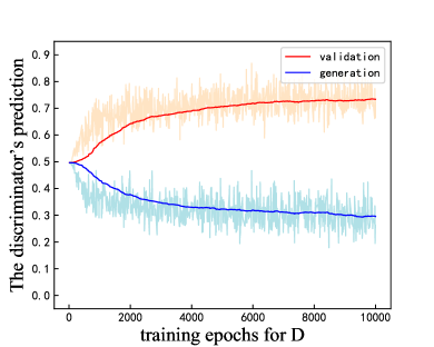
We estimate the distributional difference caused by the MLE-based generators. We first train the generator for epochs and then train until it converges (it is trained for 10 thousand epochs). For example, following (Nie et al., 2019), we train for 150 epochs, and at that time, the PPL is the smallest value measured by the validation set. Then, is trained following the procedure in section 3. Figure 2 shows the results on the EMNLP dataset. From this figure, we can see that (1) convergences after about 5,000 epochs. (2) There is always everywhere. (3) When it convergences, the is 0.7 and is 0.3. More results are illustrated in appendix B.1.
Considering the smoothed value on one batch rather than the prediction on the whole data, we use the convergence discriminator to predict on the all validation data and generated data 444According to section 3, we sample generated instances as much as test instances.. Table 1 summaries the discrepancy across two models and two datasets. It shows that the difference between real text and generated text is huge.
| Model | Dataset | Accuracy | ||
|---|---|---|---|---|
| SeqGAN | COCO | 0.42 | 0.44 | 0.71 |
| EMNLP | 0.57 | 0.47 | 0.78 | |
| RelGAN | COCO | 0.64 | 0.45 | 0.82 |
| EMNLP | 0.52 | 0.31 | 0.76 |
4.3 Could the detected discrepancy by improve the generator?
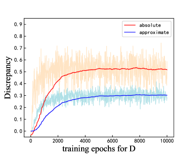
In this section, we will explore whether the above discrepancy detected by in pre-training could improve . It should be noted that the is well pre-trained. We select out the best pre-train epochs for . It is updated according to the signals from the . In order to verify the effect of those feedback signals, we generate many instances rather only several batch-size ones are used to adjust the generator’s parameters.
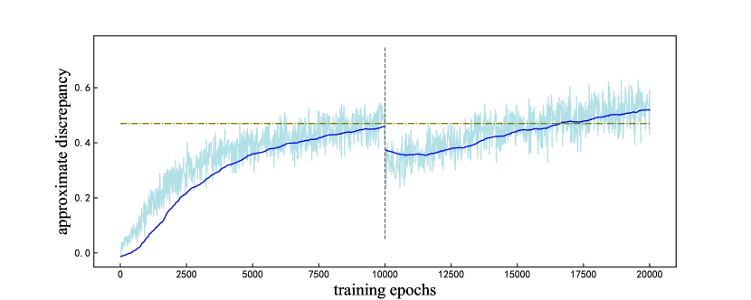
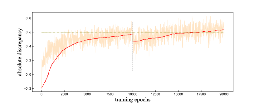
Then, fixing , we re-train with 10,000 epochs to get a new convergence discriminator, named , for computing two distributional functions according to equation 9 and 11. Unfortunately, in the view of absolute discrepancy or approximated discrepancy, the discrepancy always overpass the original value which is computed in pre-training. This demonstrates that the generator is not improved yet. Figure 3 illustrates a comparison. More experimental results are shown in appendix B.2.
Besides following (Zhu et al., 2018), We propose a new methods train . Rather than all the generated instances are used to update , only the ones who are assigned relative high scores by are used. We denote it as HW. The reason is that we think the higher score instances maybe more informative than the lower ones. In fact, only the relative low scores samples used to adjust the generator is also experimented. Regretfully, all of them fail. Table 3 list the discrepancy across two datasets. It again demonstrated that the absolute measure is necessary. Appendix B.3 show the results of several thresholds are set for selecting out more informative generated instances.
| Dataset | COCO | EMNLP | ||||||||
|---|---|---|---|---|---|---|---|---|---|---|
| pre-Train | 0.42 | 0.57 | ||||||||
| #samples | 0.1S | 0.5S | 1S | 2S | 5S | 0.1S | 0.5S | 1S | 2S | 5S |
| random | 0.52 | 0.45 | 0.54 | 0.53 | 0.55 | 0.68 | 0.68 | 0.67 | 0.67 | 0.67 |
| 0.60 | 0.58 | 0.54 | 0.54 | 0.72 | 0.77 | 0.76 | 0.73 | 0.76 | 0.73 | |
| 0.44 | 0.56 | 0.58 | 0.60 | 0.55 | 0.68 | 0.67 | 0.66 | 0.63 | 0.66 | |
| 0.52 | 0.51 | 0.47 | 0.54 | 0.58 | 0.66 | 0.57 | 0.60 | 0.64 | 0.62 | |
| 0.68 | 0.46 | 0.50 | 0.44 | 0.58 | 0.66 | 0.60 | 0.59 | 0.60 | 0.62 | |
4.4 A third party discriminator evaluates these language GANs
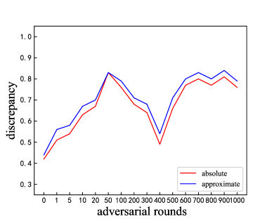
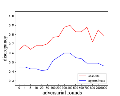
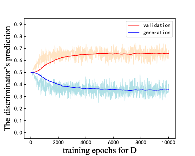
In order to evaluate different adversarial learning’s GANs, we use a third party discriminator which is a clone of the discriminator in its counterpart language GAN except for the parameters’ values. Given a round, we train many epochs (making sure it convergence) with real text and the generated text at this round. Then, two distributional functions are computed according to its prediction. Figure 4 shows the result. In the view of both approximate discrepancy and absolute discrepancy, the difference of the distribution on real text and generated text does not decrease with more adversarial learning rounds are adapted. Once again, it shows that the approach of the existing language GANs can not improve text generation.
5 Related Work
Many GAN-based models are proposed to improve traditional neural language model. SeqGAN (Yu et al., 2017) is the first one and tries by attacking the non-differential issue by resorting to RL. By applying policy gradient (Sutton et al., 2000) method, it optimizes the LSTM generator with rewards received through Monte Carlo (MC) sampling. Many researchers, such as RankGAN (Lin et al., 2017), MailGAN (Tong et al., 2017) follow this way although its in-effective in MC search. The RL-free model, for an example GSGAN (Jang et al., 2017), contains applying continuous approximating softmax function and working on latent continuous space directly. TextGAN (Salimans et al., 2016) adds Maximum Mean Discrepancy to the original objective of GAN based on feature matching. RelGAN (Nie et al., 2019) is a state-of-the-art model which uses relation memory (Santoro et al., 2018), which allows for interactions between memory slots by using the self-attention mechanism (Vaswani et al., 2017). We select out SeqGAN and RelGAN as representatives for experiment. The results show that the adversarial learning does not work for either of these models.
Caccia et al. (2019) first argues the current evaluation measures correlate with human judgment (Cífka et al., 2018) is treacherous. They furthermore propose temperature sweep which evaluates model at many temperature settings rather than only one. By using this metric, they find a well-adjust language model can beat those considered language GANs. Semeniuta et al. (2018) and He et al. (2019) also argues GAN-based models are weaker than a LM, because they observe the impact of exposure bias is not severe. He et al. (2019) furtherly quantify the exposure bias by using conditional distribution. Neither designing a better metric nor showing the weakness of the language GANs, we try to investigate language GANs in mechanism and quantify the discrepancy between real texts and generated texts both in pre-train and adversarial learning.
6 Conclusion and Future work
We present two directly metric functions to measure the discrepancy between real text and generated text. It must be noted that they are independent of any text generation method including GANs-based. Numerous experiments show that this discrepancy does exist. We try some methods to update the parameters of generator according to the detected discrepancy signals. Unfortunately, the distributional difference between real data and generated data does not decrease. It is hard to improve generator with these signals. Finally, We use a third part discriminator to evaluate the effectiveness of GAN and find with more adversarial learning epochs, the discrepancy increases rather than decreasing. It shows the existing language GANs do not work at all.
acknowledgments
We thank Hong Yang for running codes in GPU server. We also thank Diana McCarthy for suggestions on the text. This work is supported by the National Natural Science Foundation of China (61373056).
References
- Bengio et al. (2015) Samy Bengio, Oriol Vinyals, Navdeep Jaitly, and Noam Shazeer. Scheduled sampling for sequence prediction with recurrent neural networks. In NeurIPS, 2015.
- Caccia et al. (2019) Massimo Caccia, Lucas Caccia, William Fedus, Hugo Larochelle, Joelle Pineau, and Laurent Charlin. Language gans falling short. arXiv preprint arXiv:1811.02549, 2019.
- Chen et al. (2018) Liqun Chen, Shuyang Dai, Chenyang Tao, Dinghan Shen, Zhe Gan, Haichao Zhang, Yizhe Zhang, and Lawrence Carin. Adversarial text generation via feature-mover’s distance. In NeurIPS, 2018.
- Cífka et al. (2018) Ondrej Cífka, Aliaksei Severyn, Enrique Alfonseca, and Katja Filippova. Eval all, trust a few, do wrong to none: Comparing sentence generation models. CoRR, abs/1804.07972, 2018. URL http://arxiv.org/abs/1804.07972.
- d’Autume et al. (2019) Cyprien d’Autume, Mihaela Rosca, Jack Rae, and Shakir Mohamed. Training language gans from scratch. In NeurIPS, 2019.
- Fedus et al. (2018) William Fedus, Ian Goodfellow, and Andrew M. Dai. Maskgan: Better text generation via filling in the ______. In ICLR, 2018.
- Goodfellow et al. (2014) Ian J Goodfellow, Jean Pouget-Abadie, Mehdi Mirza, Xu Bing, David Warde-Farley, Sherjil Ozair, Aaron Courville, and Yoshua Bengio. Generative adversarial nets. In NeurIPS, 2014.
- Guo et al. (2018) Jiaxian Guo, Sidi Lu, Cai Han, Weinan Zhang, and Jun Wang. Long text generation via adversarial training with leaked information. In AAAI, 2018.
- He et al. (2016) Kaiming He, Xiangyu Zhang, Shaoqing Ren, and Jian Sun. Deep residual learning for image recognition. In CVPR, 2016.
- He et al. (2019) Tianxing He, Jingzhao Zhang, Zhiming Zhou, and James Glass. Quantifying exposure bias for neural language generation. arXiv preprint arXiv:1905.10617, 2019.
- Hochreiter & Schmidhuber (1997) Sepp Hochreiter and Jürgen Schmidhuber. Long short-term memory. Neural computation, 9(8):1735–1780, 1997.
- Jang et al. (2017) Eric Jang, Shixiang Gu, and Ben Poole. Categorical reparameterization with gumbel-softmax. In ICLR, 2017.
- Kim (2014) Yoon Kim. Convolutional neural networks for sentence classification. In EMNLP, 2014.
- Li et al. (2017) Jiwei Li, Will Monroe, Tianlin Shi, Sébatian Jean, Alan Ritter, and Jurafsky Dan. Adversarial learning for neural dialogue generation. In EMNLP, 2017.
- Lin et al. (2017) Kevin Lin, Dianqi Li, Xiaodong He, Zhengyou Zhang, and Ming Ting Sun. Adversarial ranking for language generation. arXiv preprint arXiv:1705.10929, 2017.
- Nie et al. (2019) Weili Nie, Narodytska Nina, and Ankit Patel. Relgan: Relational generative adversarial networks for text generation. In ICLR, 2019.
- Radford et al. (2019) Alec Radford, Jeffrey Wu, Rewon Child, David Luan, Dario Amodei, and Ilya Sutskever. Language models are unsupervised multitask learners. Technical report, 2019.
- Salimans et al. (2016) Tim Salimans, Ian Goodfellow, Wojciech Zaremba, Vicki Cheung, Alec Radford, and Xi Chen. Improved techniques for training gans. In NeurIPS, 2016.
- Santoro et al. (2018) Adam Santoro, Ryan Faulkner, David Raposo, Jack Rae, Mike Chrzanowski, Theophane Weber, Daan Wierstra, Oriol Vinyals, Razvan Pascanu, and Timothy Lillicrap. Relational recurrent neural networks. In NeurIPS, 2018.
- Semeniuta et al. (2018) Stanislau Semeniuta, Aliaksei Severyn, and Sylvain Gelly. On accurate evaluation of gans for language generation. arXiv preprint arXiv:1806.04936, 2018.
- Shi et al. (2018) Zhan Shi, Xinchi Chen, Xipeng Qiu, and Xuanjing Huang. Toward diverse text generation with inverse reinforcement learning. In IJCAI, pp. 4361–4367, 2018.
- Sutton et al. (2000) Richard S Sutton, David A McAllester, Satinder P Singh, and Yishay Mansour. Policy gradient methods for reinforcement learning with function approximation. In NeurIPS, pp. 1057–1063, 2000.
- Tong et al. (2017) Che Tong, Yanran Li, Ruixiang Zhang, R Devon Hjelm, and Yoshua Bengio. Maximum-likelihood augmented discrete generative adversarial networks. arXiv preprint arXiv:1702.07983, 2017.
- Vaswani et al. (2017) Ashish Vaswani, Noam Shazeer, Niki Parmar, Jakob Uszkoreit, Llion Jones, Aidan N. Gomez, Lukasz Kaiser, and Illia Polosukhin. Attention is all you need. In NeurIPS, 2017.
- Williams (1992) Ronald J Williams. Simple statistical gradient-following algorithms for connectionist reinforcement learning. Machine learning, 8(3-4):229–256, 1992.
- Wu et al. (2016) Yonghui Wu, Mike Schuster, Zhifeng Chen, Quoc V. Le, Mohammad Norouzi, Wolfgang Macherey, Maxim Krikun, Cao Yuan, Gao Qin, and Klaus Macherey. Google’s neural machine translation system: Bridging the gap between human and machine translation. arXiv preprint arXiv:1609.08144, 2016.
- Xu et al. (2018) Jingjing Xu, Xuancheng Ren, Junyang Lin, and Xu Sun. Diversity-promoting gan: A cross-entropy based generative adversarial network for diversified text generation. In EMNLP, 2018.
- Xu et al. (2015) Kelvin Xu, Jimmy Ba, Ryan Kiros, Kyunghyun Cho, Aaron Courville, Ruslan Salakhutdinov, Richard Zemel, and Yoshua Bengio. Show, attend and tell: Neural image caption generation with visual attention. arXiv preprint arXiv:1502.03044, 2015.
- Yu et al. (2017) Lantao Yu, Weinan Zhang, Jun Wang, and Yong Yu. Seqgan: Sequence generative adversarial nets with policy gradient. In AAAI, 2017.
- Zhu et al. (2018) Yaoming Zhu, Sidi Lu, Zheng Lei, Jiaxian Guo, Weinan Zhang, Jun Wang, and Yu Yong. Texygen: A benchmarking platform for text generation models. In SIGIR, 2018.
Appendix A Formula induction
We show the derivation of Equation 11,
| (12) | ||||
where .
Appendix B Appendix B
B.1 The rest three examples in pre-train.
B.2 The discrepancy comparison on the EMNLP dataset between pre-training and updated LM.
B.3 The comparison of the approximate discrepancy between random and HW.
| Dataset | COCO | EMNLP | ||||||||
|---|---|---|---|---|---|---|---|---|---|---|
| pre-Train | 0.44 | 0.47 | ||||||||
| #samples | 0.1S | 0.5S | 1S | 2S | 5S | 0.1S | 0.5S | 1S | 2S | 5S |
| random | 0.57 | 0.50 | 0.58 | 0.58 | 0.60 | 0.55 | 0.52 | 0.50 | 0.52 | 0.53 |
| 0.65 | 0.62 | 0.59 | 0.60 | 0.75 | 0.64 | 0.62 | 0.61 | 0.61 | 0.61 | |
| 0.49 | 0.60 | 0.62 | 0.64 | 0.56 | 0.51 | 0.50 | 0.49 | 0.49 | 0.49 | |
| 0.57 | 0.55 | 0.51 | 0.58 | 0.62 | 0.49 | 0.46 | 0.45 | 0.45 | 0.44 | |
| 0.55 | 0.55 | 0.50 | 0.61 | 0.47 | 0.47 | 0.45 | 0.45 | 0.45 | 0.46 | |
Appendix C Generated sentences on COCO image captions dataset
.
| the ground and sink are under the window of a pink covered pot . |
| a toilet sitting next to a toilet next to a green organized kitchen . |
| the bathroom contains a mop that rolls of flowers next to the vanity do two sinks . |
| a vehicle trailer meeting a corner of a street . |
| a small dog is sitting in a purse with text . |
| two men are riding an outside of the window of a street |
| a porcelain tea pot by a window |
| a humongous jumbo jet with chain chair on the ground . |
| large white bus some luggage onto one the other smiling no front tire . |
| a wooden ship with rusted heater flying high in a sky . |
| the side outside with a giraffe doors |
| the bathroom has a pedestal table with pots on it |
| bathroom with wooden cabinets and a washer , curtain and bottles growing on the flooring . |
| the side of a person looks at a woman on the back seat . |
| a bottle of whiskey in the bathroom with broken toilet |
| a ramp extends to the top of an air mattress . |
| a photograph of a palm wall in the glass ’s lap top . |
| a smiley face stand with 4 per gallon . |
| several bicycles parked stuffed in a display using it . |
| two dogs on top of a car at an amusement table . |
| a white airplane flying above someone with his friend parked behind it terminal . |
| a bathroom water from a shower with cobbler and pink tile walls . |
| a toilet is bathroom with multiple monitors paper . |
| a red fire hydrant displaying the woman in a park and many headlights . |
| a tiled bathroom with a claw view of toilet and soap dispenser |
| a group of ripe bananas in their hands on the back seat . |
| a motorcycle parked next to a stone building next to the road . |
| an airplane flies low to people aboard a boat with a cemetery a frisbee . |
| a bath room with a toilet behind it |
| a homemade cake in home bathroom has a sink , a , shower , and a window . |
| a truck is shown as the parking lot corner . |
| a bathroom is lit with foods such as : to a web job graze . |
| porcelain toilet in a blue toilet seat . |
| a simple white bathroom with a large white fridge , and shower . |
| a large delta passenger airplane flying through a cloudy sky . |
| a bathroom with a mirror , dishwasher , dishwasher , and tub/shower . |
| a blue plane is walking as seen all towards the usual number of tonic . |
| two adorable chubby dogs in a group of pots |
| four airplanes sitting on top of a building in the blue sky . |
| horse is racing on his motorcycle while maintenance are walking next to the river . |
| an image of a old bathroom with a bottle of spirits suggest tuscan decor , laptop . |
| an outdoor art bus is facing toward another snowboarder |
| a kitchen filled with in tables and two computer monitors . |
| this is an image of a motorcycle parked down by a bench . |
| a crowd of people sitting on a bench next to street |
| an electronic cat in a mens restroom next to multiple dark and pans along under a screen table . |
| two woman in her phone next to a vehicle . |
| a person riding a motor moped at a playground . |
| two dirty dog standing in front of a car . |
| a white bathtub sits next to a mirror in a small closed . |
| a white metal structure with a backpack on top . |
| a bath tub next to the toilet in middle of a nice plate . |
| rams lights and need onto the outside of a zoo . |
| an airplane parked on the ground in front of a building . |
| a white vw car passing in front of a car . |
| an airplane flying over an airport terminal . |
| two people riding bikes on an outdoor from police officer . |
| an old propeller airplane parked off . |
| a man standing down by side on a street . |
| a image of a toilet , mirror and painting on the wall |
| two toilets walking a lipstick , a television . |
| two doves sit on a bathroom counter with wooden cabinets and a bucket . |
| this enclosure has a white toilet next to the sink . |
| the dining area is wide two people riding her back to carve above them . |
| two men stand with all line of street using indoors . |
| a boy wearing travel and his motorcycle outside a town outside . |
| a person brushing her teeth with her hair holding a stove . |
| a white bathtub sitting in a bathroom with no cabinets . |
| a bath room with two counter preparing food . |
| a man holding up a market stand by the ground . |
| a kitchen has large round glass serving and cabinets . |
| a woman standing outside of a black car . |
| a bathroom has an island in the middle granite glass . |
| a large passenger jet flying over an airport next to the street . |
| a tiger cat sitting on top of a window looking very clean . |
| bicyclists holding a flip phone next to the aircraft . |
| a walk opened in the bathroom with a jungle theme . |
| the sink has white appliances with a child . |
| a kitchen with a chrome toilet next to bathtub . |
| man standing in a blue park looking sidewalk next to a brown horse against a group of electrical boxes . |
| an old parked motorcycle with its kickstand down to . |
| a messy bathroom with a tub , in the sink and the mirror with no privacy . |
| a an open kitchen tucked in a public kitchen . |
| a white brown kitchen with bowls on a counter top counter . |
| a woman standing in red liquid under a small water fountain . |
| a view above the toilet roll a sink with a stove . |
| a couple of chefs up in a kitchen preparing food . |
| a bathroom with a toilet , and mirrors from its reflection in a large sink . |
| a bath room with a tub and refrigerator . |
| a group of traffic light with people skiing in the mist |
| two dogs are huddled together a screen corner on a wall . |
| wild animals grazing in the center of a blue sky . |
| a woman holds a spoon by off a road . |
| a kitchen with toiletries in the just darts . |
| motor sandwich and ride to turn across a road . |
| a man crossing a traffic in an oriental city |
| women turning her phone food prepares food . |
| two stuffed animals are laptop , dishwasher , and a sink . |
| a toilet in front of a window in a white room . |
| large woman , on snowboards at an open purse |
| an image of a sink , trash can . |