Training-Free Uncertainty Estimation for
Dense Regression:
Sensitivity as a Surrogate
Abstract
Uncertainty estimation is an essential step in the evaluation of the robustness for deep learning models in computer vision, especially when applied in risk-sensitive areas. However, most state-of-the-art deep learning models either fail to obtain uncertainty estimation or need significant modification (e.g., formulating a proper Bayesian treatment) to obtain it. Most previous methods are not able to take an arbitrary model off the shelf and generate uncertainty estimation without retraining or redesigning it. To address this gap, we perform a systematic exploration into training-free uncertainty estimation for dense regression, an unrecognized yet important problem, and provide a theoretical construction justifying such estimations. We propose three simple and scalable methods to analyze the variance of outputs from a trained network under tolerable perturbations: infer-transformation, infer-noise, and infer-dropout. They operate solely during the inference, without the need to re-train, re-design, or fine-tune the models, as typically required by state-of-the-art uncertainty estimation methods. Surprisingly, even without involving such perturbations in training, our methods produce comparable or even better uncertainty estimation when compared to training-required state-of-the-art methods.
Introduction
Deep neural networks have achieved remarkable or even super-human performance in many tasks (Krizhevsky, Sutskever, and Hinton 2012; He et al. 2015; Silver et al. 2016). While most previous work in the field has focused on improving accuracy in various tasks, in several risk-sensitive areas such as autonomous driving (Chen et al. 2015) and healthcare (Zhang et al. 2019), reliability and robustness are arguably more important and interesting than accuracy.
Recently, several novel approaches have been proposed to take into account an estimation of uncertainty during training and inference (Huang et al. 2018). Some use probabilistic formulations for neural networks (Graves 2011; Hernández-Lobato and Adams 2015; Wang, Shi, and Yeung 2016; Shekhovtsov and Flach 2018) and model the distribution over the parameters (weights) and/or the neurons. Such formulations naturally produce distributions over the possible outputs (Ilg et al. 2018; Yang, Hu, and Ramanan 2019). Others utilize the randomness induced during training and inference (e.g., dropout and ensembling) to obtain an uncertainty estimation (Gal and Ghahramani 2016; Lakshminarayanan, Pritzel, and Blundell 2017; Kendall, Badrinarayanan, and Cipolla 2015).
All methods above require specific designs or a special training pipeline in order to involve the uncertainty estimation during training. Unfortunately, there are many cases where such premeditated designs or pipelines cannot be implemented. For example, if one wants to study the uncertainty of trained models released online, retraining is not always an option, especially when only a black-box model is provided or the training data is not available. Moreover, most models are deterministic and do not have stochasticity. A straightforward solution is to add dropout layers into proper locations and finetune the model (Gal and Ghahramani 2016). However, this is impractical for many state-of-the-art and published models, especially those trained on large datasets (e.g. ImageNet (Deng et al. 2009)) with a vast amount of industrial computing resources. In addition, models that have already been distilled, pruned, or binarized fall short of fitting re-training (Han, Mao, and Dally 2015; Hou, Yao, and Kwok 2016).
To fill this gap, we identify the problem of training-free uncertainty estimation: how to obtain an uncertainty estimation of any given model without re-designing, re-training, or fine-tuning it. We focus on two scenarios: black-box uncertainty estimation (BBUE), where one has access to the model only as a black box, and gray-box uncertainty estimation (GBUE), where one has access to intermediate-layer neurons of the model (but not the parameters). Our work is a systematic exploration of this unrecognized yet important problem.
We propose a set of simple and scalable training-free methods to analyze the variance of the output from a trained network, shown in Fig. 1. Our main idea is to add a tolerable perturbation into inputs or feature maps during inference and use the variance of the output as a surrogate for uncertainty estimation.
The first method, which we call infer-transformation, is to apply a transformation that exploits the natural characteristics of a CNN – it is variant to input transformation such as rotation (Cohen and Welling 2016). Transformations have been frequently used as data augmentation but rarely evaluated for uncertainty estimation. The second method, infer-noise, is to inject Gaussian noise with a zero-mean and a small standard deviation into intermediate-layer neurons. The third one, called infer-dropout, is to perform inference-time dropout in a chosen layer. Although at first blush infer-dropout is similar to MC-dropout, where dropout is performed during both training and inference in the same layers, they are different in several aspects: (1) Infer-dropout is involved only during inference. (2) Infer-dropout can be applied to arbitrary layers, even those without dropout training. Surprisingly, we find that even without involving dropout during training, infer-dropout is still comparable to, or even better than, MC-dropout for the purpose of uncertainty estimation.
In our paper, we focus on regression tasks. Note that for classification tasks, the softmax output is naturally a distribution. Methods that use entropy for uncertainty estimation qualify as a training-free method and have outperformed MC-Dropout (Bahat and Shakhnarovich 2018; Gal and Ghahramani 2016; Hendrycks and Gimpel 2016; Wang et al. 2019) (see the Supplement for experiment results). Regression tasks are more challenging than classification problems since there is no direct output distribution. (Kuleshov, Fenner, and Ermon 2018; Song et al. 2019). And our major contributions are:
-
1.
We perform a systematic exploration of training-free uncertainty estimation for regression models and provide a theoretical construction justifying such estimations.
-
2.
We propose simple and scalable methods, infer-transformation, infer-noise and infer-dropout, using a tolerable perturbation to effectively and efficiently estimate uncertainty.
-
3.
Surprisingly, we find that our methods are able to generate uncertainty estimation comparable or even better than training-required baselines in real-world large-scale dense regression tasks.
Related Work
Probabilistic Neural Networks for Uncertainty Estimation. Probabilistic neural networks consider the input and model parameters as random variables which take effect as the source of stochasticity (Nix and Weigend 1994; Welling and Teh 2011; Graves 2011; Hernández-Lobato and Adams 2015; Wang, Shi, and Yeung 2016). Traditional Bayesian neural networks model the distribution over the parameters (weights) (MacKay 1992; Hinton and Van Camp 1993; Graves 2011; Welling and Teh 2011) and obtain the output distribution by marginalizing out the parameters. Even with recent improvement (Balan et al. 2015; Hernández-Lobato and Adams 2015), one major limitation is that the size of network at least doubles under this assumption, and the propagation with a distribution is usually computationally expensive. Another set of popular and efficient methods (Gal and Ghahramani 2016; Teye, Azizpour, and Smith 2018) formulate dropout (Srivastava et al. 2014) or batch normalization (Ioffe and Szegedy 2015) as approximations to Bayesian neural networks. For example, MC-dropout (Gal and Ghahramani 2016) injects dropout into some layers during both training and inference (Tsymbalov et al. 2019). Unlike most models that disable dropout during inference, MC-dropout feed-forwards the same example multiple times with dropout enabled, in order to form a distribution on the output. Meanwhile, other works (Wang, Shi, and Yeung 2016; Shekhovtsov and Flach 2018) propose sampling-free probabilistic neural networks as a lightweight Bayesian treatment for neural networks.
Non-probabilistic Neural Networks for Uncertainty Estimation. Other strategies (Zhao, Ma, and Ermon 2020) such as deep ensemble (Lakshminarayanan, Pritzel, and Blundell 2017; Huang et al. 2017a; Ashukha et al. 2020) train an ensemble of neural networks from scratch, where some randomness is induced during the training process, i.e. the initial weight is randomly sampled from a distribution. During inference, these networks will generate a distribution of the output. Though simple and effective, training multiple networks costs even more time and memory than Bayesian neural networks. Another efficient method log likelihood maximization (LLM) is to train the network to have both original outputs and uncertainty predictions, by jointly optimizing both (Zhang et al. 2019; Poggi et al. 2020). Besides the methods above focusing on uncertainty in classification models; there are also works investigating uncertainty in regression models (Kuleshov, Fenner, and Ermon 2018; Song et al. 2019; Zelikman et al. 2020). However, all methods above requires re-training, introduces heavy implementation overhead, and sometimes makes the optimization process more challenging.
Methodology
Three Cases on Parameter Accessibility. We distinguish among three cases based on accessibility of the original model. 1. Black-box case: the model is given as a trained black box without any access to its internal structure. 2. Gray-box case: the internal representations (feature maps) of the model is accessible (while the parameters are not) and can be modified during inference. 3. White-box case: the model is available for all modifications (e.g. its weights can be modified, which requires training). In this paper we focus on the black-box and gray-box cases, for which we offer, correspondingly, two classes of methods. For the black-box case, we propose infer-transformation, which exploits the model’s dependence on input transformations, e.g. rotations/flips. For the grey-box case, we propose infer-noise and infer-dropout, which introduce an internal embedding/representation manipulation - injecting a noise layer or a dropout layer during inference. These three methods are illustrated in Fig. 1. The description of our methods and a theoretical construction are presented as below.
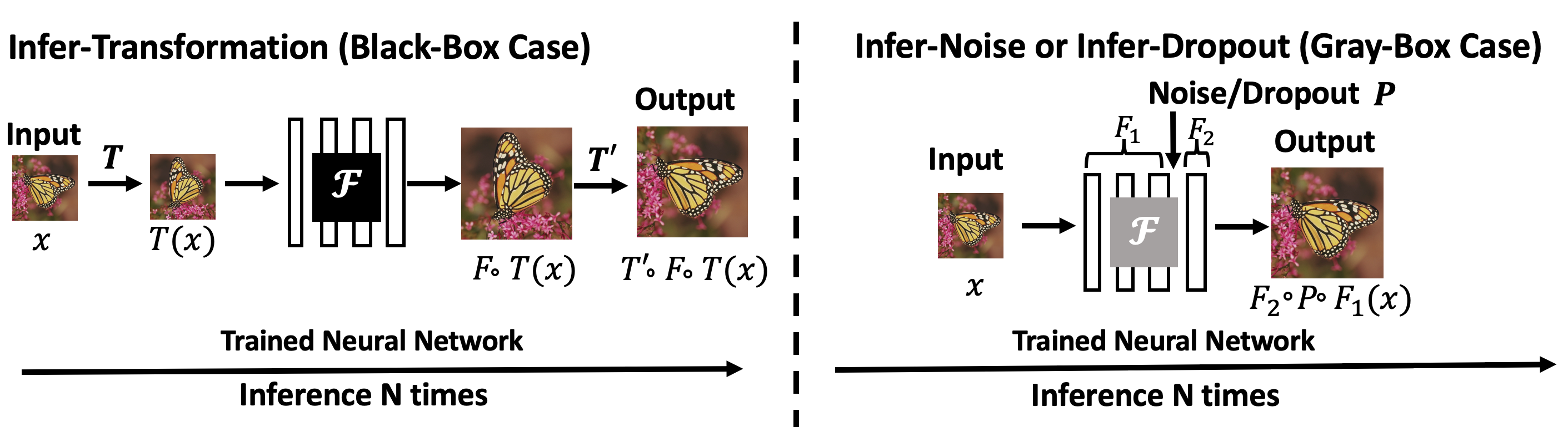
Black-Box Uncertainty Estimation: Infer-Transformation
Given a black-box model, we explore the behavior of the outputs for different transformed versions of the input. Specifically, we transform the input with tolerable perturbations, e.g. perturbations that do not cause significant increase in the loss, and then use the variance of the perturbed outputs as estimated uncertainty. Here we focus on transformations that preserve pertinent characteristics of the input, such as rotations, flips, etc. Formally, given an input image X, our measured uncertainty is defined as , where is a transformation, is ’s inverse operation, and is a function representing the black-box neural network. is a sample from the perturbed output distribution. Note that it is possible to sample , where happens to be a 360-degree rotation.
Gray-Box Uncertainty Estimation: Infer-Noise and Infer-Dropout
Given a gray-box model, we consider another class of methods for generating multiple outputs from a distribution: randomly perturbing latent codes. Compared with the black-box case, this provides finer granularity on modulating the perturbation strength to ensure tolerability. Specifically, we propose infer-noise, which introduces Gaussian noise at an intermediate layer of the trained model, and infer-dropout, which uses dropout instead. For infer-noise, the noise will be added to the feature maps of a certain layer. This noise is randomly sampled multiple times during inference to form a set of diverse outputs. For infer-dropout, random dropout is performed for multiple forwards to generate output samples, the variance of which is then used as uncertainty estimation. Formally, given an input image X, our measured uncertainty is defined as , where is sampled from a perturbation set (e.g. Gaussian noise with ). is the function of network layers before the perturbation , represents network layers after , and is the gray-box network . is a sample from the perturbed output distribution. Note that it is possible to sample , where happens to be a perturbation noise of all zeros.
Correlation between Sensitivity and Uncertainty
In this section, we provide a theoretical justification for using sensitivity as a surrogate of uncertainty. Specifically, we will show that sensitivity and uncertainty have a non-negative correlation in a simplified setting with mild assumptions.
Notations. We use random variables and to denote the input data point and target label. and denote the model predictions of original and perturbed input, respectively. Furthermore, and denote the expectation and the variance of the model prediction of perturbations of a certain input . We call (or for short) the sensitivity of the model for the input . We use to denote the error of the model’s prediction. We consider as an indicator of the model’s uncertainty: a larger prediction error means that the model should have been less uncertain at this input. We use to denote the Pearson correlation between two random variables.
Assumptions. To analyze the correlation between sensitivity and uncertainty, we make the following assumptions:
-
1.
Heterogeneous perturbation: . This assumption says the model prediction given an unperturbed input ‘looks like’ a random draw from the model predictions of perturbed inputs.
-
2.
Random bias: . This assumption says the bias of the model prediction ‘looks like’ white noise with bounded variance .
-
3.
Independence: and . Basically, we assume the randomness in , and the sensitivity are statistically independent.
Empirically, we find these assumptions are satisfied to some degree (see detailed results in the Supplement).
Correlation Analysis. The following theorem analyzes the correlation between sensitivity and uncertainty .
Theorem 1.
With the above assumptions satisfied, we have:
| (1) |
where and .
We make several remarks on the derived correlation between sensitivity and uncertainty.
-
1.
: It holds because and always have non-negative correlation. It means statistically, sensitivity has the same ‘direction’ as uncertainty.
-
2.
is monotonically decreasing w.r.t. to : It holds since decreases as grows. Consider two extremes: (a) (the prediction has no bias at all): then degenerates to , leading to the highest sensitivity-uncertainty correlation. (b) (the prediction has unbounded bias). then degenerates to , leading to zero sensitivity-uncertainty correlation.
-
3.
is monotonically decreasing w.r.t. to : It holds since decreases as grows. Note that is bounded (between and ) and that indicates the variability of the sensitivity. Specifically, is equivalent to , meaning that the sensitivity is constant everywhere. In this extreme case, sensitivity has zero correlation with uncertainty. Fortunately, in practice, we find sensitivity always varies with different inputs. The variation is often large, leading relatively small. As a result, sensitivity usually has a high correlation with uncertainty.
-
4.
: Using sensitivity as a surrogate can at most achieve pixel-wise correlation of . For block-wise, patch-wise, and image-level correlation (see the Experiment Section for definitions), we can apply similar analysis to obtain higher upper bounds.
Theorem 1 establishes the correlation between sensitivity and uncertainty . In our experiments, we use as sensitivity for convenience since it achieves similar performance.
Epistemic Uncertainty and Aleatoric Uncertainty
Our model can estimate both epistemic uncertainty and aleatoric Uncertainty (Kendall and Gal 2017). As in practice, the model is not able to perfectly fit infinite data – all variants of augmented “data” (including both data inputs and intermediate features) applied with different perturbations – then we will get a nonzero variance, which represents the epistemic uncertainty. In the meanwhile, our methods can also be applied to measure aleatoric uncertainty for accessible data. Given a data input fed into a trained model under multiple tolerable perturbations, outputs with higher variance than those from other data inputs represent this data input with relatively high aleatoric uncertainty. And we demonstrate to use of such properties to implement active learning, and results are shown in the Supplement.
Experiments
In this section, we evaluate our three proposed approaches in two representative real-world large-scale dense regression tasks, super single image resolution, and monocular depth estimation.
Single Image Super Resolution
The task of Single Image Super Resolution (SR) is to reconstruct a high-resolution (HR) image from a low-resolution (LR) input. Here we focus on analyzing the state-of-the-art SRGAN model (Ledig et al. 2017), which can restore photo-realistic high-quality images. SRGAN always outputs deterministic restorations since the conditional GAN (Mirza and Osindero 2014) used in this model involves no latent variable sampling. However, we can still evaluate its uncertainty with our proposed methods.
We apply our methods to estimate uncertainty in one open-source version of this work (Dong et al. 2017). The package provides two models trained with different loss functions: 1) SRresnet model with loss and 2) SRGAN model with a combination of loss and adversarial loss. We evaluate our methods on both models in the black-box/gray-box settings.
Infer-Transformation. For infer-transformation, we apply a rotation of degrees () as well as horizontal flip to the LR input, feed it into the trained model during the inference, and apply the inverse transformation to its output. We could generate at most 8 samples using this strategy, and then calculate the pixel-wise variance.
Infer-Noise. In infer-noise, we take the trained model and add a Gaussian-noise layer, which has standard deviation and mean , at different locations (layers). We choose 4 different locations for noise injection, including the layers right after the input and some intermediate layers (see details in the Supplement. For each experiment, we only add the noise into one layer with a specific value. Sample numbers of 8 and 32 are evaluated.
Infer-Dropout. In infer-dropout, we take the trained model and add a dropout layer with varied dropout rates. We choose the dropout rate from the set and use the same set of locations as the infer-noise. For each experiment, we only add the layer into one location with one specific dropout rate. Sample numbers of 8 and 32 are evaluated.
Baselines. We compare our methods with three training-required baselines. The first baseline is MC-dropout (Gal and Ghahramani 2016) with a dropout rate . For each experiment, we add a dropout layer only into one location with one dropout rate during training. The same dropout rate is used for sampling during inference. We try different sample numbers of 8 and 32. The second baseline is deep ensemble (Lakshminarayanan, Pritzel, and Blundell 2017). We follow this work to train ensembles as and networks, respectively. We train these networks with the same number of epochs until they converge. During inference, each of them generates a single deterministic output, with or samples generated in total. The third baseline is a sampling-free method log-likelihood maximization (LLM) (Zhang et al. 2019; Poggi et al. 2020), where a network is trained to predict an output distribution with log-likelihood maximization.
Monocular Depth Estimation
For depth estimation (Postels et al. 2019; Kendall and Gal 2017), we use one of the commonly applied models based on a fully convolutional residual network (FCRN) (Laina et al. 2016). We directly use the trained model released by the original author; this is consistent with the scenarios of black-box and gray-box cases since the code for training is not released. We evaluate the model on NYU Depth Dataset V2. For infer-transformation, we avoid applying 90-degree rotation to input, since the orientation is strong prior to predicting depth which can violate the tolerability, and only apply horizontal flip to generate samples for uncertainty estimation. For infer-dropout, we choose two locations (intermediate layers) to add the dropout layer. For infer-noise, we choose three locations to add the noise layer (two intermediate layers and one layer before the final FC layer). Then we conduct similar experiments as described in the SR task. For the baseline MC-dropout, note that the model has a dropout layer before the final fully connected (FC) layer during training, we directly perform sampling from the existing dropout layer. Sample numbers of and are evaluated for both infer-dropout and infer-noise, see details in the Supplement.
| SRGAN model: Super Resolution | ||||||||||||||
| Condition | Training Free (Ours) | Training Required | ||||||||||||
| Prediction | Original Output | Outputs Mean | ||||||||||||
| Method | Infer-trans | Infer-drop | Infer-noise | MC-drop1 | MC-drop2 | Ensemble | LLM | |||||||
| Samples | 4 | 8 | 8 | 32 | 8 | 32 | 8 | 32 | 8 | 32 | 4 | 8 | 0 | |
| AUSE | mean | 0.006 | 0.006 | 0.013 | 0.013 | 0.016 | 0.016 | 0.008 | 0.009 | 0.007 | 0.007 | 0.018 | 0.020 | 0.035 |
| patch | 0.021 | 0.022 | 0.029 | 0.030 | 0.040 | 0.039 | 0.029 | 0.029 | 0.025 | 0.025 | 0.033 | 0.033 | 0.044 | |
| block | 0.023 | 0.023 | 0.032 | 0.031 | 0.044 | 0.043 | 0.030 | 0.029 | 0.028 | 0.028 | 0.033 | 0.033 | 0.042 | |
| pixel | 0.128 | 0.121 | 0.154 | 0.141 | 0.173 | 0.162 | 0.141 | 0.131 | 0.137 | 0.129 | 0.152 | 0.144 | 0.137 | |
| Corr | mean | 0.931 | 0.930 | 0.884 | 0.882 | 0.774 | 0.780 | 0.942 | 0.943 | 0.938 | 0.936 | 0.692 | 0.694 | 0.484 |
| patch | 0.765 | 0.770 | 0.722 | 0.731 | 0.590 | 0.598 | 0.748 | 0.755 | 0.734 | 0.741 | 0.674 | 0.677 | 0.565 | |
| block | 0.757 | 0.767 | 0.717 | 0.730 | 0.579 | 0.592 | 0.735 | 0.747 | 0.698 | 0.710 | 0.651 | 0.664 | 0.588 | |
| pixel | 0.367 | 0.394 | 0.323 | 0.376 | 0.245 | 0.288 | 0.339 | 0.390 | 0.330 | 0.379 | 0.290 | 0.326 | 0.393 | |
| NLL | 17.910 | 9.332 | 4.889 | 4.804 | 4.899 | 4.791 | 6.804 | 6.013 | 6.365 | 5.541 | 11.520 | 5.994 | 1.320 | |
| SRresnet model: Super Resolution | ||||||||||||||
| Condition | Training Free (Ours) | Training Required | ||||||||||||
| Prediction | Original Output | Outputs Mean | ||||||||||||
| Method | Infer-trans | Infer-drop | Infer-noise | MC-drop1 | MC-drop2 | Ensemble | LLM | |||||||
| Samples | 4 | 8 | 8 | 32 | 8 | 32 | 8 | 32 | 8 | 32 | 4 | 8 | 0 | |
| AUSE | mean | 0.044 | 0.044 | 0.042 | 0.043 | 0.067 | 0.066 | 0.041 | 0.047 | 0.036 | 0.039 | 0.073 | 0.066 | 0.036 |
| patch | 0.045 | 0.044 | 0.048 | 0.047 | 0.055 | 0.055 | 0.046 | 0.045 | 0.040 | 0.041 | 0.066 | 0.066 | 0.037 | |
| block | 0.047 | 0.045 | 0.049 | 0.048 | 0.062 | 0.061 | 0.048 | 0.046 | 0.041 | 0.042 | 0.073 | 0.070 | 0.031 | |
| pixel | 0.164 | 0.153 | 0.165 | 0.155 | 0.190 | 0.181 | 0.163 | 0.152 | 0.150 | 0.144 | 0.194 | 0.185 | 0.133 | |
| Corr | mean | 0.340 | 0.359 | 0.401 | 0.404 | 0.056 | 0.055 | 0.408 | 0.379 | 0.527 | 0.512 | 0.016 | 0.048 | 0.622 |
| patch | 0.501 | 0.520 | 0.508 | 0.518 | 0.371 | 0.385 | 0.535 | 0.545 | 0.547 | 0.542 | 0.323 | 0.361 | 0.648 | |
| block | 0.462 | 0.486 | 0.498 | 0.509 | 0.358 | 0.370 | 0.505 | 0.521 | 0.531 | 0.529 | 0.274 | 0.286 | 0.673 | |
| pixel | 0.237 | 0.269 | 0.258 | 0.303 | 0.172 | 0.216 | 0.264 | 0.309 | 0.288 | 0.322 | 0.184 | 0.206 | 0.393 | |
| NLL | 107.243 | 43.071 | 5.155 | 4.955 | 4.941 | 4.788 | 8.430 | 7.221 | 8.018 | 6.688 | 13.559 | 7.906 | 1.422 | |
| FCRN model: Depth Estimation | ||||||||||
| Condition | Training Free (Ours) | Training Required | ||||||||
| Prediction | Original Output | Outputs Mean | ||||||||
| Method | Infer-trans | Infer-drop | Infer-noise | MC-drop1 | MC-drop2 | |||||
| Samples | 2 | 2 | 8 | 2 | 8 | 2 | 8 | 2 | 8 | |
| AUSE | mean | 0.051 | 0.044 | 0.041 | 0.046 | 0.041 | 0.062 | 0.062 | 0.060 | 0.062 |
| patch | 0.106 | 0.109 | 0.092 | 0.108 | 0.091 | 0.127 | 0.126 | 0.122 | 0.125 | |
| block | 0.056 | 0.057 | 0.047 | 0.053 | 0.045 | 0.065 | 0.065 | 0.063 | 0.065 | |
| pixel | 0.165 | 0.168 | 0.135 | 0.167 | 0.134 | 0.208 | 0.193 | 0.207 | 0.193 | |
| Corr | mean | 0.596 | 0.630 | 0.677 | 0.651 | 0.708 | 0.473 | 0.471 | 0.469 | 0.469 |
| patch | 0.324 | 0.306 | 0.409 | 0.312 | 0.411 | 0.258 | 0.268 | 0.266 | 0.269 | |
| block | 0.354 | 0.354 | 0.449 | 0.364 | 0.447 | 0.215 | 0.220 | 0.220 | 0.221 | |
| pixel | 0.208 | 0.182 | 0.284 | 0.188 | 0.288 | 0.075 | 0.134 | 0.076 | 0.134 | |
| NLL | 8.634 | 8.443 | 4.889 | 3.526 | 1.006 | 12.365 | 9.842 | 12.503 | 9.866 | |
Experiment Results
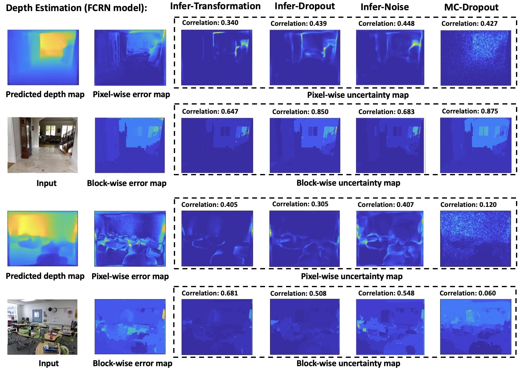
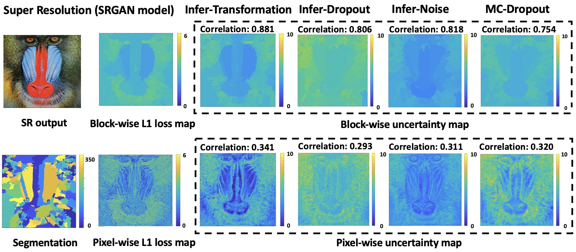
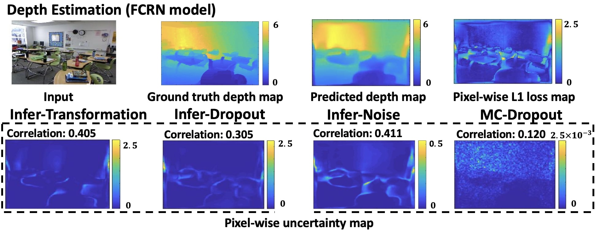
Qualitative Results. Fig. 2 shows some qualitative results for an example image in the SR task. We can see that the variance maps generated in our task are consistent with the level of ambiguity. Specifically, in our methods, high variance occurs in areas with high randomness and high frequency. For the depth estimation task shown in Fig. 3, high variance usually occurs in the area with high spatial resolution and large depth. As expected, these high-variance areas usually correspond to large prediction errors.
Evaluation Metrics. Commonly used metrics to evaluate uncertainty estimation include Brier score (BS), expected calibration error (ECE), and negative log-likelihood (NLL) (Lakshminarayanan, Pritzel, and Blundell 2017; Guo et al. 2017). However, BS and ECE are for classification tasks only and hence not applicable in our setting. We therefore use the following metrics for evaluations: (1) NLL, which is defined in regression tasks by assuming a Gaussian distribution. However, note that NLL depends on not only the quality of uncertainty estimation but also the prediction accuracy itself. Therefore contrary to previous belief, we argue that it is not an ideal metric for evaluating uncertainty estimation. (2) Area Under the Sparsification Error (AUSE), which quantifies how much uncertainty estimation coincides with the true errors (Ilg et al. 2018). (3) Correlation between the estimated uncertainty and the error. Here we define four variants of correlation (see details in the Supplement): pixel-wise, mean, block-wise, and patch-wise correlations to evaluate performance at the pixel, image, block, and patch levels, respectively. The intuition is that in many situations it is more instructive and meaningful when uncertainty is visualized in each region (e.g. a region with a possible tumor for a medical imaging application). Note that block-wise correlation depends on specific segmentation algorithms, while patch-wise correlation defines regions in an algorithm-independent way. Similarly, we also define four evaluation forms for AUSE.
For our training-free methods, these metrics are computed between uncertainty and the error from the original model (without perturbation), because we will still use the original model for prediction. For training-required methods such as MC-dropout (i.e. MC-drop2 in Table 1) (Gal and Ghahramani 2016), deep ensemble (Lakshminarayanan, Pritzel, and Blundell 2017) and log likelihood maximization (LLM) (Zhang et al. 2019; Poggi et al. 2020), the mean of output samples are used as prediction. Meanwhile, we also evaluate another MC-dropout variant, denoted as MC-drop1, where the output of the original model is used as prediction, to be consistent with training-free methods. The evaluation results using metrics described above are shown in Table 1 and Table 2.
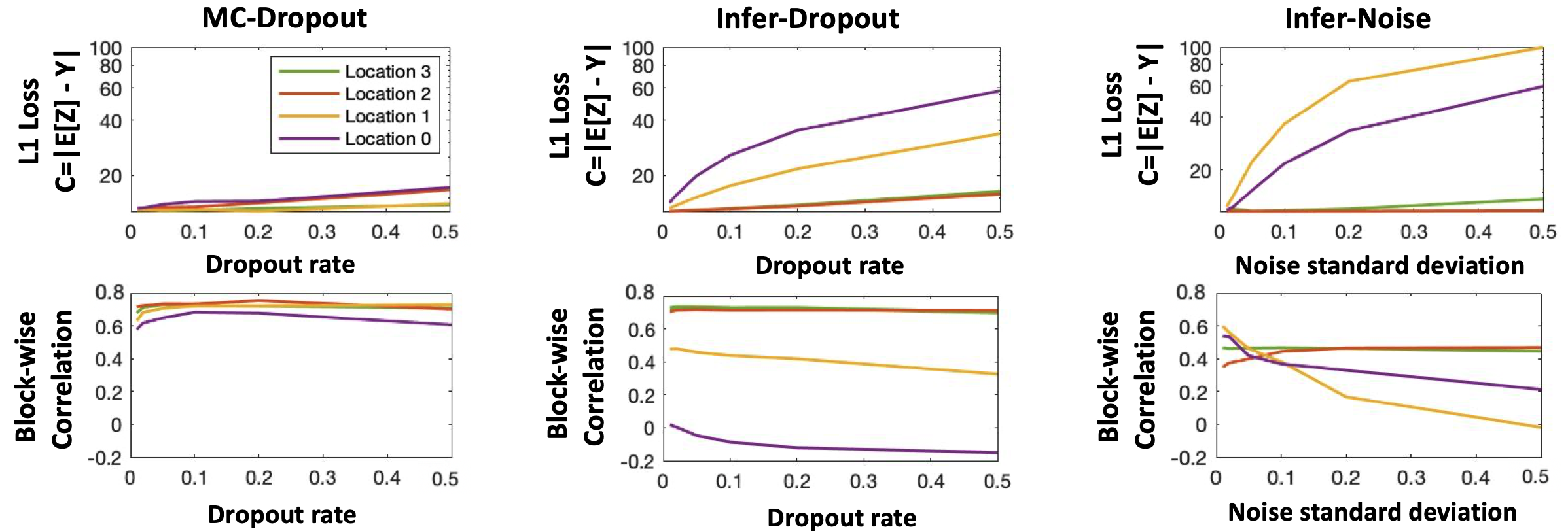
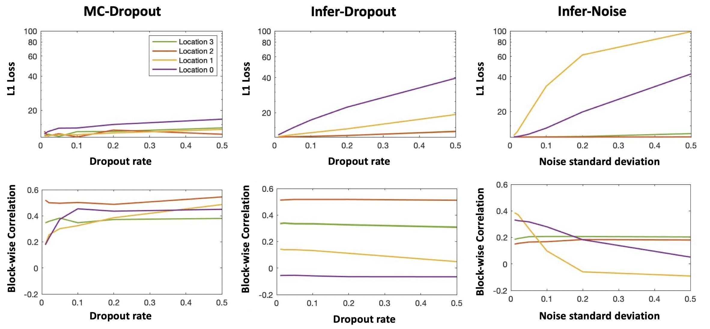
The Role of Tolerable Perturbations. Tolerable perturbations play a crucial role in obtaining effective uncertainty estimation. Better tolerability means smaller decrease in accuracy after perturbation. Fig. 4 shows the correlation for different amount of perturbations (noise or dropout) in different locations, and the corresponding predictive performance (evaluated as loss) after perturbations. As we can see, the optimal cases to generate uncertainty maps with high correlation require that should remain small after perturbation (high tolerability). Generally, our experiments suggest that perturbations leading to less than relative drop of performance work well for uncertainty estimation. This observation verifies Theorem 1. Specifically, note that by definition (in the ‘Notations’ paragraph), ; therefore given the ‘random bias’ assumption (in the ‘Assumptions’ paragraph) that , the expectation of over all the pixels . By Remark 2 of Theorem 1, is monotonically decreasing w.r.t. to , which is linear to .
Interestingly, different methods have different ways of achieving high tolerability: (1) For MC-dropout, involving dropout during training increases the robustness of models against perturbations, keeping the loss relatively small after adding dropout layer in most locations during inference; (2) for infer-dropout, adding dropout layer in intermediate locations (i.e. location 2 and location 3) where the information is the most redundant (He et al. 2014), can effectively alleviate disturbance; (3) for infer-noise, adding noise with small standard deviation effectively limits the perturbation level. More interestingly, we further find that for both MC-dropout and infer-dropout, adding perturbation in intermediate layers is usually the optimal choice for uncertainty estimation. Applying infer-dropout in these intermediate layers, we could achieve comparable or even better performance compared to training-required baselines. For infer-noise, locations do not have a similar effect; one can therefore further tune the noise strength to achieve a higher correlation.
Applications
We find several applications that can be benefited from the uncertainty estimated in our methods. The first application is to improve the quality of SR results. We propose a novel method that takes the pixel-wise uncertainty map as a weight term for the regression loss while keeping the original adversarial loss; this could provide a more photo-realistic SR output with finer structures and sharper edges. Another application is active learning (Gal, Islam, and Ghahramani 2017), which aims to use uncertainty to choose the next batch of data for annotation. Our result shows that active learning based on our generated uncertainty maps can provide a higher data efficiency (details are shown in the Supplement).
Conclusion & Discussion
In this work, we perform a systematic exploration into training-free uncertainty estimation for dense regression, an unrecognized yet important problem, and provide a theoretical construction justifying such estimations. We propose three simple, scalable, and effective methods, i.e. infer-transformation, infer-noise, and infer-dropout, for uncertainty estimation in both black-box and gray-box cases. Surprisingly, our training-free methods achieve comparable or even better results compared to training-required state-of-the-art methods. Furthermore, we demonstrate adding tolerable perturbations is the key to generating high-quality uncertainty maps for all methods we studied. Meanwhile, we find the optimal choice of the training-free uncertainty estimation method is task-dependent. We suggest using infer-transformation for super-resolution and infer-noise for depth estimation. The limitation of our works is the requirement of well-trained neural networks. And our methods are not applicable to deep neural networks with random guesses.
Acknowledgement
The authors thank the reviewers/SPC/AC for the constructive comments to improve the paper. We thank Intel, Analog Devices, Thermo Fisher Scientific, NSF grants 1563880 and 1607189 to support this project. Lu Mi is partially supported by MathWorks Fellowship. Hao Wang is partially supported by NSF Grant IIS-2127918 and an Amazon Faculty Research Award.
References
- Aganj et al. (2018) Aganj, I.; Harisinghani, M. G.; Weissleder, R.; and Fischl, B. 2018. Unsupervised medical image segmentation based on the local center of mass. Scientific reports, 8(1): 13012.
- Ashukha et al. (2020) Ashukha, A.; Lyzhov, A.; Molchanov, D.; and Vetrov, D. 2020. Pitfalls of in-domain uncertainty estimation and ensembling in deep learning. arXiv preprint arXiv:2002.06470.
- Bahat and Shakhnarovich (2018) Bahat, Y.; and Shakhnarovich, G. 2018. Confidence from Invariance to Image Transformations. arXiv preprint arXiv:1804.00657.
- Balan et al. (2015) Balan, A. K.; Rathod, V.; Murphy, K. P.; and Welling, M. 2015. Bayesian dark knowledge. In NIPS.
- Chen et al. (2015) Chen, C.; Seff, A.; Kornhauser, A.; and Xiao, J. 2015. Deepdriving: Learning affordance for direct perception in autonomous driving. In ICCV, 2722–2730.
- Cohen and Welling (2016) Cohen, T.; and Welling, M. 2016. Group equivariant convolutional networks. In ICML, 2990–2999.
- Deng et al. (2009) Deng, J.; Dong, W.; Socher, R.; Li, L.-J.; Li, K.; and Fei-Fei, L. 2009. Imagenet: A large-scale hierarchical image database. In CVPR, 248–255.
- Dong et al. (2017) Dong, H.; Supratak, A.; Mai, L.; Liu, F.; Oehmichen, A.; Yu, S.; and Guo, Y. 2017. TensorLayer: A Versatile Library for Efficient Deep Learning Development. ACM Multimedia.
- Gal and Ghahramani (2016) Gal, Y.; and Ghahramani, Z. 2016. Dropout as a bayesian approximation: Representing model uncertainty in deep learning. In ICML, 1050–1059.
- Gal, Islam, and Ghahramani (2017) Gal, Y.; Islam, R.; and Ghahramani, Z. 2017. Deep bayesian active learning with image data. In ICML, 1183–1192.
- Graves (2011) Graves, A. 2011. Practical Variational Inference for Neural Networks. In NIPS.
- Guo et al. (2017) Guo, C.; Pleiss, G.; Sun, Y.; and Weinberger, K. Q. 2017. On calibration of modern neural networks. In ICML, 1321–1330.
- Han, Mao, and Dally (2015) Han, S.; Mao, H.; and Dally, W. J. 2015. Deep compression: Compressing deep neural networks with pruning, trained quantization and huffman coding. In ICLR.
- He et al. (2015) He, K.; Zhang, X.; Ren, S.; and Sun, J. 2015. Delving deep into rectifiers: Surpassing human-level performance on imagenet classification. In ICCV, 1026–1034.
- He et al. (2016) He, K.; Zhang, X.; Ren, S.; and Sun, J. 2016. Deep residual learning for image recognition. In CVPR, 770–778.
- He et al. (2014) He, T.; Fan, Y.; Qian, Y.; Tan, T.; and Yu, K. 2014. Reshaping deep neural network for fast decoding by node-pruning. In ICASSP, 245–249.
- Hendrycks and Gimpel (2016) Hendrycks, D.; and Gimpel, K. 2016. A baseline for detecting misclassified and out-of-distribution examples in neural networks. arXiv preprint arXiv:1610.02136.
- Hernández-Lobato and Adams (2015) Hernández-Lobato, J. M.; and Adams, R. 2015. Probabilistic Backpropagation for Scalable Learning of Bayesian Neural Networks. In ICML.
- Hinton and Van Camp (1993) Hinton, G. E.; and Van Camp, D. 1993. Keeping the neural networks simple by minimizing the description length of the weights. In COLT.
- Hou, Yao, and Kwok (2016) Hou, L.; Yao, Q.; and Kwok, J. T. 2016. Loss-aware binarization of deep networks.
- Huang et al. (2017a) Huang, G.; Li, Y.; Pleiss, G.; Liu, Z.; Hopcroft, J. E.; and Weinberger, K. Q. 2017a. Snapshot ensembles: Train 1, get m for free. arXiv preprint arXiv:1704.00109.
- Huang et al. (2017b) Huang, G.; Liu, Z.; Van Der Maaten, L.; and Weinberger, K. Q. 2017b. Densely connected convolutional networks. In Proceedings of the IEEE conference on computer vision and pattern recognition, 4700–4708.
- Huang et al. (2018) Huang, P.-Y.; Hsu, W.-T.; Chiu, C.-Y.; Wu, T.-F.; and Sun, M. 2018. Efficient uncertainty estimation for semantic segmentation in videos. In Proceedings of the European Conference on Computer Vision (ECCV), 520–535.
- Ilg et al. (2018) Ilg, E.; cCiccek, Ö.; Galesso, S.; Klein, A.; Makansi, O.; Hutter, F.; and Brox, T. 2018. Uncertainty Estimates and Multi-hypotheses Networks for Optical Flow. In ECCV, 677–693.
- Ioffe and Szegedy (2015) Ioffe, S.; and Szegedy, C. 2015. Batch normalization: Accelerating deep network training by reducing internal covariate shift. arXiv preprint arXiv:1502.03167.
- Kendall, Badrinarayanan, and Cipolla (2015) Kendall, A.; Badrinarayanan, V.; and Cipolla, R. 2015. Bayesian segnet: Model uncertainty in deep convolutional encoder-decoder architectures for scene understanding. arXiv preprint arXiv:1511.02680.
- Kendall and Gal (2017) Kendall, A.; and Gal, Y. 2017. What uncertainties do we need in bayesian deep learning for computer vision? In NIPS, 5574–5584.
- Krizhevsky, Sutskever, and Hinton (2012) Krizhevsky, A.; Sutskever, I.; and Hinton, G. E. 2012. Imagenet classification with deep convolutional neural networks. In NIPS, 1097–1105.
- Kuleshov, Fenner, and Ermon (2018) Kuleshov, V.; Fenner, N.; and Ermon, S. 2018. Accurate uncertainties for deep learning using calibrated regression. In International Conference on Machine Learning, 2796–2804.
- Laina et al. (2016) Laina, I.; Rupprecht, C.; Belagiannis, V.; Tombari, F.; and Navab, N. 2016. Deeper depth prediction with fully convolutional residual networks. In 3DV, 239–248.
- Lakshminarayanan, Pritzel, and Blundell (2017) Lakshminarayanan, B.; Pritzel, A.; and Blundell, C. 2017. Simple and scalable predictive uncertainty estimation using deep ensembles. In NIPS, 6402–6413.
- Ledig et al. (2017) Ledig, C.; Theis, L.; Huszár, F.; Caballero, J.; Cunningham, A.; Acosta, A.; Aitken, A.; Tejani, A.; Totz, J.; Wang, Z.; et al. 2017. Photo-realistic single image super-resolution using a generative adversarial network. In CVPR, 4681–4690.
- MacKay (1992) MacKay, D. 1992. A practical Bayesian framework for backprop networks. Neural computation.
- Mirza and Osindero (2014) Mirza, M.; and Osindero, S. 2014. Conditional generative adversarial nets. arXiv preprint arXiv:1411.1784.
- Nix and Weigend (1994) Nix, D. A.; and Weigend, A. S. 1994. Estimating the mean and variance of the target probability distribution. In Proceedings of 1994 ieee international conference on neural networks (ICNN’94), volume 1, 55–60. IEEE.
- Poggi et al. (2020) Poggi, M.; Aleotti, F.; Tosi, F.; and Mattoccia, S. 2020. On the uncertainty of self-supervised monocular depth estimation. In Proceedings of the IEEE/CVF Conference on Computer Vision and Pattern Recognition, 3227–3237.
- Postels et al. (2019) Postels, J.; Ferroni, F.; Coskun, H.; Navab, N.; and Tombari, F. 2019. Sampling-free Epistemic Uncertainty Estimation Using Approximated Variance Propagation. arXiv preprint arXiv:1908.00598.
- Ronneberger, Fischer, and Brox (2015) Ronneberger, O.; Fischer, P.; and Brox, T. 2015. U-net: Convolutional networks for biomedical image segmentation. In MICCAI, 234–241.
- Shekhovtsov and Flach (2018) Shekhovtsov, A.; and Flach, B. 2018. Feed-forward Propagation in Probabilistic Neural Networks with Categorical and Max Layers. In ICLR.
- Silver et al. (2016) Silver, D.; Huang, A.; Maddison, C. J.; Guez, A.; Sifre, L.; Van Den Driessche, G.; Schrittwieser, J.; Antonoglou, I.; Panneershelvam, V.; Lanctot, M.; et al. 2016. Mastering the game of Go with deep neural networks and tree search. nature, 529(7587): 484.
- Song et al. (2019) Song, H.; Diethe, T.; Kull, M.; and Flach, P. 2019. Distribution calibration for regression. In International Conference on Machine Learning, 5897–5906.
- Srivastava et al. (2014) Srivastava, N.; Hinton, G.; Krizhevsky, A.; Sutskever, I.; and Salakhutdinov, R. 2014. Dropout: a simple way to prevent neural networks from overfitting. JMLR, 15(1): 1929–1958.
- Teye, Azizpour, and Smith (2018) Teye, M.; Azizpour, H.; and Smith, K. 2018. Bayesian uncertainty estimation for batch normalized deep networks. arXiv preprint arXiv:1802.06455.
- Tsymbalov et al. (2019) Tsymbalov, E.; Makarychev, S.; Shapeev, A.; and Panov, M. 2019. Deeper connections between neural networks and Gaussian processes speed-up active learning. arXiv preprint arXiv:1902.10350.
- Wang et al. (2019) Wang, G.; Li, W.; Aertsen, M.; Deprest, J.; Ourselin, S.; and Vercauteren, T. 2019. Aleatoric uncertainty estimation with test-time augmentation for medical image segmentation with convolutional neural networks. Neurocomputing, 338: 34–45.
- Wang, Shi, and Yeung (2016) Wang, H.; Shi, X.; and Yeung, D.-Y. 2016. Natural-parameter networks: A class of probabilistic neural networks. In NIPS, 118–126.
- Welling and Teh (2011) Welling, M.; and Teh, Y. W. 2011. Bayesian learning via stochastic gradient Langevin dynamics. In Proceedings of the 28th international conference on machine learning (ICML-11), 681–688.
- Yang, Hu, and Ramanan (2019) Yang, G.; Hu, P.; and Ramanan, D. 2019. Inferring Distributions Over Depth from a Single Image. arXiv preprint arXiv:1912.06268.
- Zelikman et al. (2020) Zelikman, E.; Healy, C.; Zhou, S.; and Avati, A. 2020. CRUDE: Calibrating Regression Uncertainty Distributions Empirically. arXiv preprint arXiv:2005.12496.
- Zhang et al. (2019) Zhang, Z.; Romero, A.; Muckley, M. J.; Vincent, P.; Yang, L.; and Drozdzal, M. 2019. Reducing Uncertainty in Undersampled MRI Reconstruction with Active Acquisition. In CVPR, 2049–2058.
- Zhao, Ma, and Ermon (2020) Zhao, S.; Ma, T.; and Ermon, S. 2020. Individual calibration with randomized forecasting. In International Conference on Machine Learning, 11387–11397.
Appendix
Proof of Theorem 1
Proof.
Putting the equations above together, we have
∎
Assumption Evaluation for Correlation Analysis
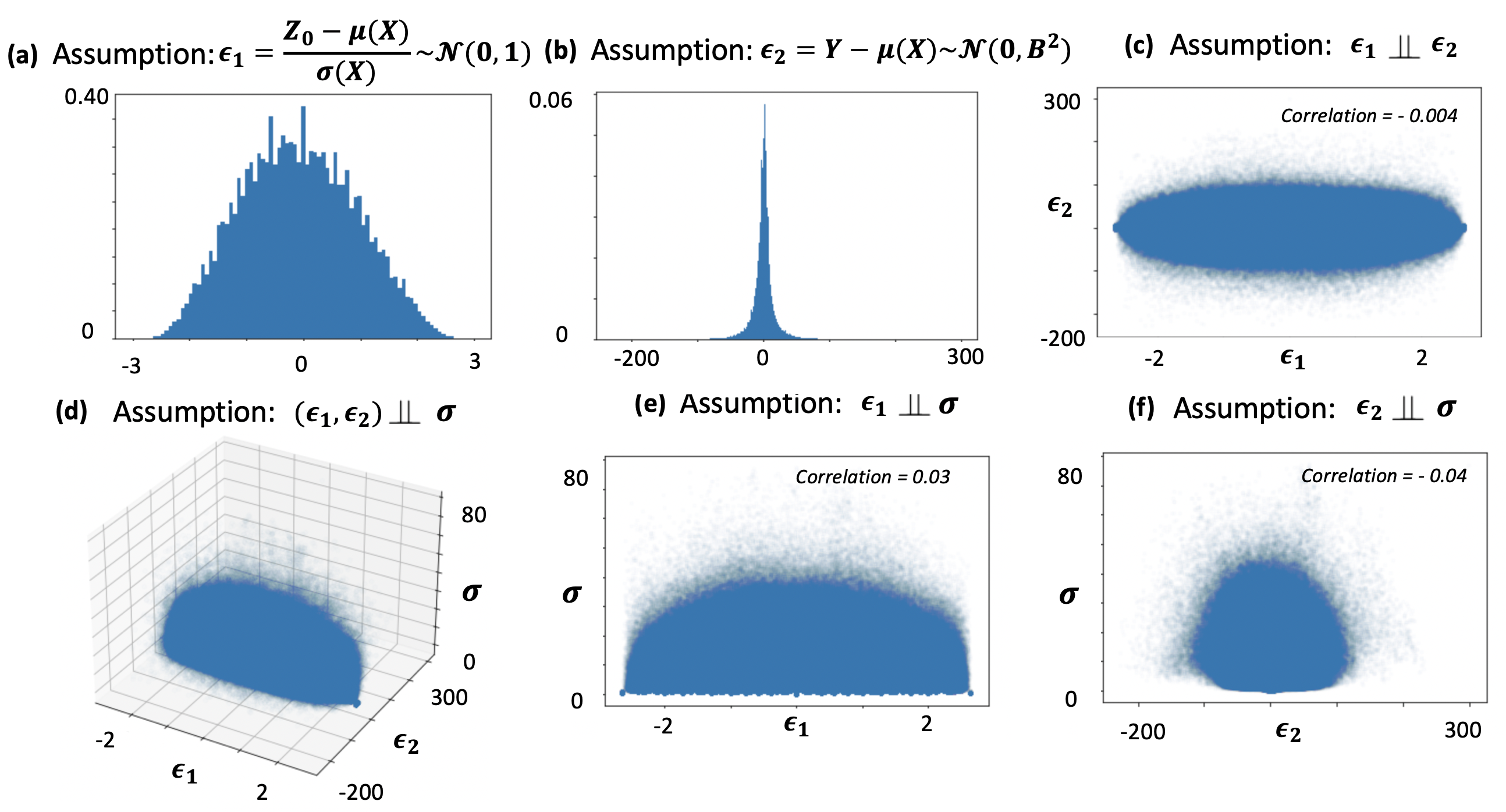
In this section, we evaluate the assumptions to perform our correlation analysis, and find most of them are satisfied to some degree. We demonstrate an example of described variables in the assumption for infer-transformation on SRGAN model in Figure 5. In (a), we show the histogram of of all pixels in the Set14, and such distribution is very close to a standard normal distribution as expected, which demonstrates our Assumption 1 (in the main paper) related to heterogeneous perturbation is satisfied. Similarly, we evaluate the random bias assumption (Assumption 2) by showing the histogram of in (b). We find this distribution is relatively close to a normal distribution , and here the measured is . In the meanwhile, we also evaluate the dependence of these random variables (Assumption 3). Figure 5(c) shows the independence assumption of and is satisfied to some degree, and the independence assumption of and is evaluated in (d), (e), (f).
Applications Benefit from Uncertainty Estimation
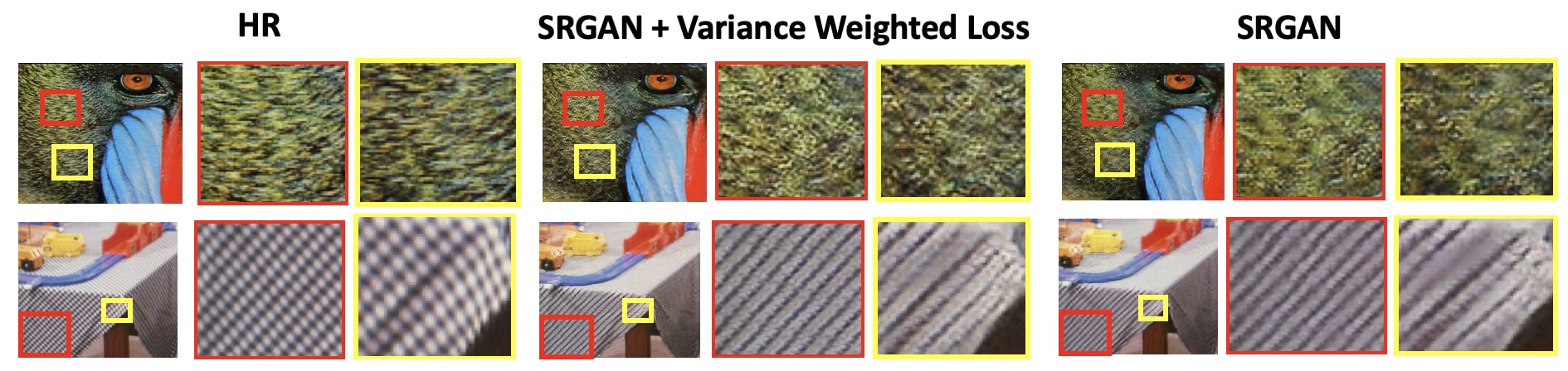
The first application is to improve the quality of SR results. We propose a novel and efficient method which takes the pixel-wise uncertainty map as a weight term for the regression loss, while keeps the original adversarial loss, which could provide a more photo-realistic SR output with finer structures and sharper edges, shown in Fig. 6. Another application is active learning (Gal, Islam, and Ghahramani 2017), which aims to use uncertainty to guide annotations, then only a small subset of data are required to improve training. We find active learning based on our generated uncertainty maps can improve the performance with more efficiency, shown in Table 3.
| Method | SSIM | PSNR | |
|---|---|---|---|
| original | 0.772 | 23.841 | 11.623 |
| random | 0.773 | 23.616 | 12.344 |
| high uncertainty | 0.790 | 23.942 | 11.497 |
Details on Network Noise/Dropout Injection
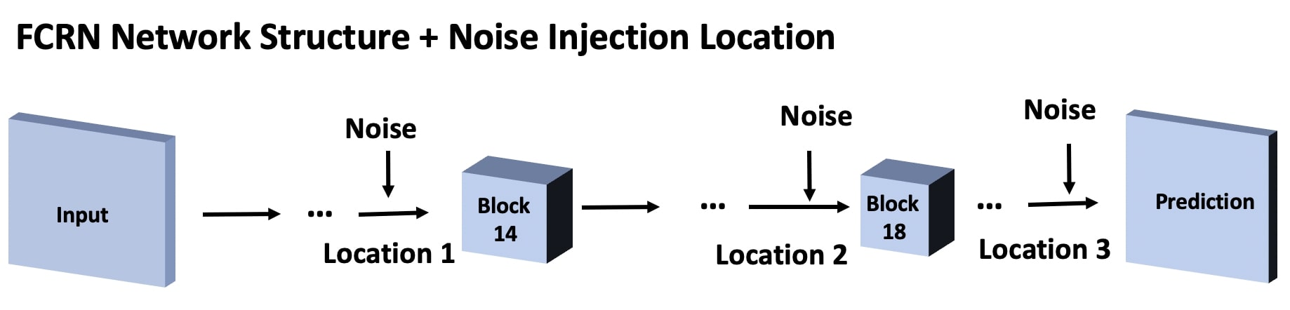
To perform uncertainty estimation using infer-noise, infer-dropout, and baseline MC-dropout on both SRGAN model and SRresnet model, we choose 4 different locations for noise injection, including the layers right after the input, as well as some intermediate layers, as shown in Fig. 7.

To perform uncertainty estimation using infer-noise and infer-dropout on FCRN model, we choose 3 different locations for noise injection, including the layers right before the output, as well as some intermediate layers, as shown in Fig. 8. For baseline MC-dropout, we choose location 3 where the dropout layer added during training for the original model.
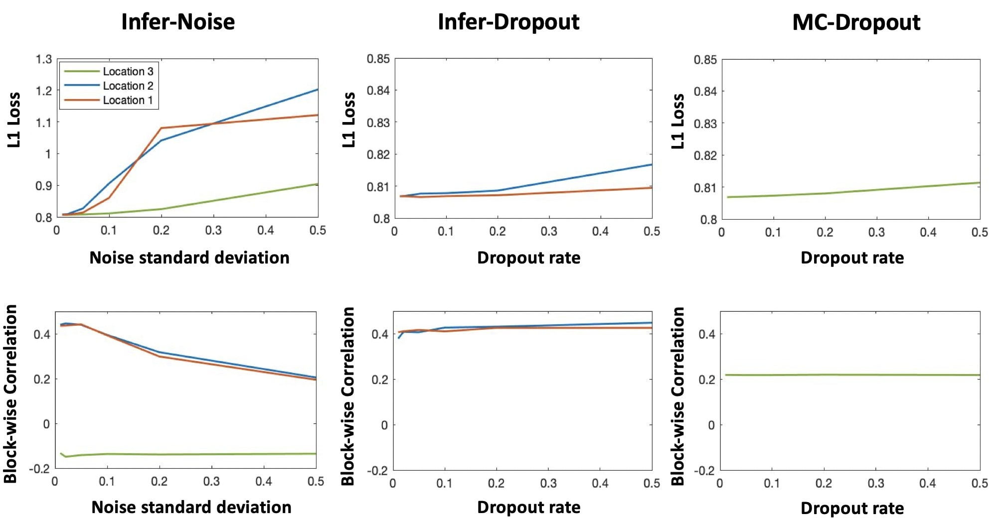
Tolerability on SRresnet and FCRN
Fig. 9 shows the perturbation on the SRresnet model, and Fig. 10 shows the perturbation on the FCRN model for depth estimation. We plot the correlation between different amount of perturbations (noise or dropout) in different locations and the corresponding predictive performance (evaluated as loss) after perturbations. For SRresnet model, We find that for both MC-dropout and infer-dropout, adding perturbation in intermediate layers is usually the optimal choice for uncertainty estimation. For infer-noise, locations do not have similar effect; one can therefore further tune the noise strength to achieve higher correlation. For FCRN model, when infer-dropout or infer-noise is applied, intermediate layers are also usually the optimal choices for uncertainty estimation. The results are consistent with that of SRGAN model.
Details on Evaluation Metrics
In this section, we provide the details for our proposed correlation-based evaluation metrics. Assuming we have N outputs given the same input from our infer-transformation, infer-drop and infer-noise, each output is represented by . Given the output image with the size of , the error we define for regression task is pixel-wise loss and loss, represented by and , where , is the corresponding coordinates of the pixel in the output image. The uncertainty (variance) estimated in these methods is also a pixel-wise value, represented by . The pixel-wise correlation is defined as . The second metric is mean correlation, the mean error is defined as the average error of a single image , correspondingly, the mean variance is defined as , the mean correlation is defined as . This metric has been used in (Zhang et al. 2019). The third metric for evaluation is the block-wise correlation – a new metric we propose in this work. To compute block-wise correlation, we need to firstly apply a local segmentation algorithm to the output of the trained model to cluster pixels with similar low-level context. Here we use the local-center-of-mass approach (Aganj et al. 2018) to perform segmentation. We denote each cluster as . The variance of pixels inside each cluster (block) is then averaged and replaced with the mean value . The block-wise loss can be calculated similarly. After that, we calculate the pixel-wise correlation of each pixels with the updated value as the block-wise correlation . For the fourth metric, patch-wise correlation, where the segmentation clusters in block-wise correlation are replaced by patches. In our analysis, each image is divided into patches. And then the patch-wise correlation is calculated with following the same rule as block-wise correlation. Besides correlation, we also define four similar metrics in terms of AUSE. More details related with the definition of AUSE are in (Ilg et al. 2018).
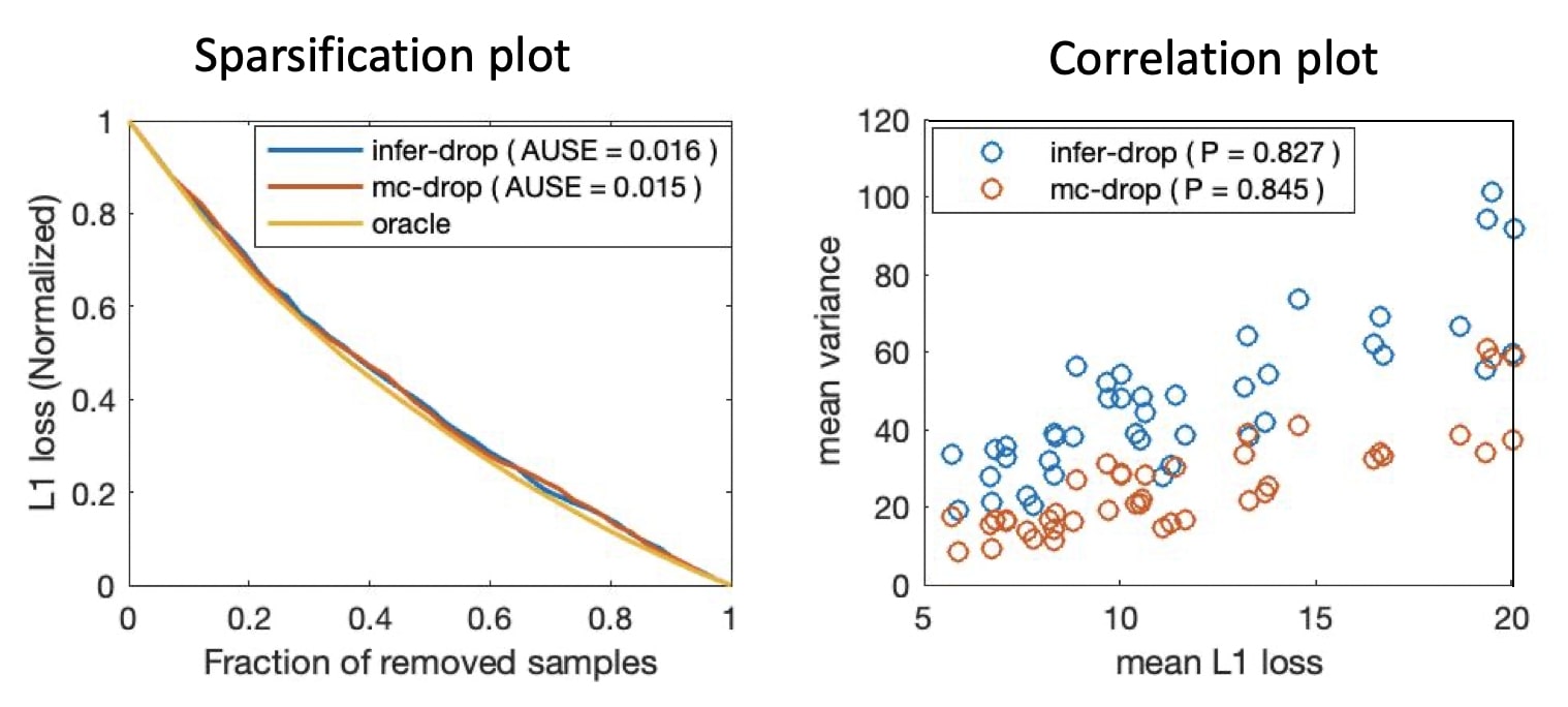
Meanwhile, as illustrated in Fig. 11, we find that sparsification error has a strong association with correlation, when the oracle sparsifications of different methods are the same. As a result, when AUSE of infer-dropout and MC-dropout (defined as MC-drop1 here) is nearly identical, correlation is almost the same.
| Densenet | UNET | Resnet | ||||
|---|---|---|---|---|---|---|
| Entropy | MC-drop | Entropy | MC-drop | Entropy | MC-drop | |
| Mean Correlation | 0.928 | 0.718 | 0.964 | 0.881 | 0.669 | 0.537 |
| Pixel-wise Correlation | 0.502 | 0.209 | 0.789 | 0.317 | – | – |
Evaluations on Classification Tasks
We compare the simple training-free method using entropy and the training-required method MC-dropout on classification tasks. For classification tasks, the most straightforward and commonly used method is to calculate the entropy of output probability as uncertainty, which already qualifies as a training-free method. We then compare it with a sampling-based and training-required method – MC-dropout, tuned on different locations and using 8 samples. Here we conduct three experiments: the first one is multi-class segmentation task using Densenet (Huang et al. 2017b) on CamVid dataset; the second one is a binary segmentation task using UNET (Ronneberger, Fischer, and Brox 2015) on a biomedical public benchmark dataset from the SNEMI3D challenge; and the third one is a classification task on CIFAR100 using ResNet (He et al. 2016). We calculate the correlation between the entropy of softmax output and the cross-entropy loss. We find that using entropy outperforms MC-dropout based on the correlation metric, as shown in Table 4.
Visualization of Uncertainty Maps
The uncertainty maps generated using infer-transformation, infer-dropout, infer-noise compared with MC-dropout, and the corresponding error maps for images are shown in Fig. 12 for the super-resolution task, and in Fig. 13 for the depth estimation task.
One interesting observation is that MC-dropout tends to capture local variance and ignore high-level semantics, partially because the dropout layer is always at the end of the network. As a result, it is difficult for MC-dropout to produce uncertainty estimates in detail-rich regions. For example, the input image in the bottom row of Fig. 13 contains a lot of details with chairs and desks. Unfortunately MC-dropout tends to ignore these details and only produce high variance in the upper half of the image (region with large depth), leading to poor correlation.