A Semi-Definite Programming Approach to Robust Adaptive MPC under State Dependent Uncertainty

Abstract

We propose an Adaptive MPC framework for uncertain linear systems to achieve robust satisfaction of state and input constraints. The uncertainty in the system is assumed additive, state dependent, and globally Lipschitz with a known Lipschitz constant. We use a non-parametric technique for online identification of the system uncertainty by approximating its graph via envelopes defined by quadratic constraints. At any given time, by solving a set of convex optimization problems, the MPC controller guarantees robust constraint satisfaction for the closed-loop system for all possible values of system uncertainty modeled by the envelope. The uncertainty envelope is refined with data using Set Membership Methods. We highlight the efficacy of the proposed framework via a detailed numerical example.

I Introduction

System modeling and identification has been an integral part of statistics and data sciences [1, 2]. In recent times, as data-driven decision making and control becomes ubiquitous [3, 4], such system identification methods are being integrated with control algorithms for control of uncertain dynamical systems. In computer science community, data driven reinforcement learning algorithms [5, 6] have been extensively utilized for policy and value function learning of uncertain systems. In control theory, if the actual model of a system is unknown, adaptive control [7, 8] strategies have been applied for simultaneous system identification and control. In such classical adaptive control methods, primarily unconstrained systems are considered, and model parameters are learned from data in terms of point estimates, while proving stability of the closed-loop system.

The concept of online model learning and adaptation has been extended to control design for systems under constraints as well. In [9], linear time invariant system dynamics matrices and the confidence intervals are learned using Ordinary Least Squares regression and imposed constraints are robustly satisfied using System Level Synthesis [10]. Lowering the conservatism of such an approach, the field of Adaptive MPC has gained attention in recent times [11, 12, 13, 14, 15]. In the aforementioned Adaptive MPC frameworks, Set Membership Method based approaches are used to obtain the sets containing all possible realizations of model uncertainty. These sets are then modified as more data becomes available. However, the model uncertainty learned is not considered as a function of system states. Work such as [16, 17, 18] extend the Adaptive MPC framework to systems with state dependent uncertainties, where set based bounds of the uncertainty is adapted using Gaussian Process (GP) regression. However, due to probabilistic nature of GP regression based estimates, there is no closed-loop constraint satisfaction guarantees in such methods. To the best of our knowledge, there has not been a unifying framework for robust MPC design in presence of state dependent system model uncertainty.

In this paper, we propose a novel approach to designing a robust Adaptive MPC algorithm for linear systems subject to state and input constraints, in presence of state dependent system uncertainty. The uncertainty is assumed globally Lipschitz, with a known Lipschitz constant. We utilize a non-parametric recursive system identification strategy [19], which identifies the graph of the uncertainty from data using its Lipschitz property. The identification is successively refined with recorded data. Our main contributions are:

• We provide set based bounds containing all possible realizations of the system uncertainty, using its Lipschitz property. This in contrast to the probabilistic nature of bounds in [16, 17, 18], due to the use of GP regression. Our uncertainty set bounds are modified successively with set intersections upon gathering new data.

• Utilizing the above bounds on system uncertainty, we synthesize a robust Adaptive MPC controller by solving convex optimization problems, satisfying imposed state and input constraints. We prove its recursive feasibility, extending feasibility guarantees of [11, 13, 15] in presence of state dependent uncertainty. We further demonstrate the validity and efficacy of the proposed approach through a detailed numerical simulation.

The paper is organized as follows: Section II formulates the robust optimization problem to be solved for the uncertain system, along with the system model and constraints. Section III contains the recursive system uncertainty adaptation framework. The tractable robust Adaptive MPC is posed in Section IV. We present numerical results in Section V.

II Problem Formulation

II-A System Model

The system is given by:

$$x_{t+1}=Ax_{t}+Bu_{t}+d(x_{t}),$$ (1)

where $x_{t}\in\mathbb{R}^{n}$ is the state at time $t$, $u_{t}\in\mathbb{R}^{m}$ is the input, $A$ and $B$ are known system matrices of appropriate dimensions, and $d(x_{t})$ constitutes un-modelled dynamics, that is, the system uncertainty, which is $L_{d}$ Lipschitz in its convex and closed domain $\mathrm{dom}(d)$ with a known $L_{d}$.

II-B Constraints

The system dynamics are subject to polytopic state and input constraints of the form:

$$\mathcal{X} =\{x\in\mathbb{R}^{n}\ |H_{x}x\leq h_{x}\},$$ (2a)

$$\mathcal{U} =\{u\in\mathbb{R}^{m}\ |H_{u}u\leq h_{u}\},$$ (2b)

where we assume $\mathcal{X}\subseteq\mathrm{dom}(d)$.

II-C Robust Optimization Problem

Our goal is to design a controller that solves the following infinite horizon optimal control problem with constraints (2)

$$\begin{array}[]{clll}\displaystyle\min_{u_{0},u_{1}(\cdot),\ldots}&\displaystyle\sum\limits_{t\geq 0}\bar{x}_{t}^{\top}Q\bar{x}_{t}+u_{t}^{\top}(\bar{x}_{t})Ru_{t}(\bar{x}_{t})\\[4.30554pt] \text{s.t.}&x_{t+1}=Ax_{t}+Bu_{t}(x_{t})+d(x_{t}),\\ &\bar{x}_{t+1}=A\bar{x}_{t}+Bu_{t}(\bar{x}_{t})+\bar{d}(\bar{x}_{t}),\\[4.30554pt] &H_{x}x_{t+1}\leq h_{x},\ ~{}\forall d(x_{t})\in\mathcal{D}(x_{t}),\\ &H_{u}u(x_{t})\leq h_{u},\ \forall d(x_{t})\in\mathcal{D}(x_{t}),\\[4.30554pt] &x_{0}=\bar{x}_{0}=x_{S},\\ &t=0,1,\ldots,\end{array}$$ (3)

where $\mathcal{D}(x_{t})$ is a state dependent compact set where the uncertainty $d(x_{t})$ is guaranteed to lie, and $\bar{d}(\bar{x}_{t})$ denotes the certainty equivalent (nominal) estimate of uncertainty at any point $\bar{x}_{t}$ along the nominal trajectory. Matrices $Q,R\succ 0$ are weight matrices. We point out that, as system (1) is uncertain, the optimal control problem (3) consists of finding input policies $[u_{0},u_{1}(\cdot),u_{2}(\cdot),\ldots]$, where $u_{t}:\mathbb{R}^{n}\ni x_{t}\mapsto u_{t}=u_{t}(x_{t})\in\mathbb{R}^{m}$. We wish to approximate solutions to optimization problem (3) by solving the following finite time constrained optimal control problem at each time $t$, in a receding horizon fashion:

$$\begin{array}[]{llll}\displaystyle\min_{u_{t|t},u_{t+1|t}(\cdot),\dots}&{\sum}_{k=t}^{t+N-1}(\bar{x}_{k|t}^{\top}Q\bar{x}_{k|t}+u_{k|t}^{\top}(\bar{x}_{k|t})Ru_{k|t}(\bar{x}_{k|t}))\\ &~{}~{}~{}~{}~{}~{}~{}~{}~{}~{}~{}~{}~{}~{}~{}~{}~{}~{}~{}~{}~{}~{}~{}~{}~{}~{}+\bar{x}_{t+N|t}^{\top}P_{N}\bar{x}_{t+N|t}\vspace{2mm}\\ \ \ \quad\text{s.t. }&{x}_{k+1|t}=A{x}_{k|t}+Bu_{k|t}(x_{k|t})+d(x_{k|t}),\\ &\bar{x}_{k+1|t}=A\bar{x}_{k|t}+Bu_{k|t}(\bar{x}_{k|t})+\bar{d}(\bar{x}_{k|t}),\vspace{.6em}\\ &H_{x}x_{k+1|t}\leq h_{x},~{}\forall d(x_{k|t})\in\mathcal{D}(x_{k|t}),\\ &H_{u}u_{k|t}(x_{k|t})\leq h_{u},~{}\forall d(x_{k|t})\in\mathcal{D}(x_{k|t}),\\ &\forall k=t,t+1,\dots t+N-1,\\ &x_{t+N|t}\in\mathcal{X}_{N},\\ &x_{t|t}=\bar{x}_{t|t}=x_{t},\end{array}$$ (4)

where $x_{k|t}$ is the predicted state after applying the predicted policy $[u_{t|t}(x_{t|t}),\dots,u_{k-1|t}(x_{k-1|t})]$ for $k=\{t+1,\dots,t+N\}$ to system (1), $\mathcal{X}_{N}$ is the terminal set and $P_{N}\succ 0$ is the terminal cost. In the following sections, we address the three crucial challenges associated to finding solutions of (4):

1. Learning and updating the uncertainty bounds $\mathcal{D}(\cdot)$ with data to obtain a nonempty $\mathcal{X}_{N}$.

2. Obtaining tractable parametrization of input policy $u(\cdot)$ to avoid searching over infinite dimensional function spaces, and

3. Ensuring robust satisfaction of (2) for all times, if tractable reformulation of (4) is feasible once.

III Uncertainty Learning and Adaptation

At every time instant $t$, we assume that we have access to measurements $d(x_{i})$ for all $i=\{0,1,\dots,t-1\}$, that is, the realizations of the uncertainty function.

III-A Successive Graph Approximation

Definition 1 (Graph)

The graph of a function $f:\mathbb{R}^{n}\rightarrow\mathbb{R}^{n}$ is defined as the set

$$G(f)=\{(x,f(x))\in\mathbb{R}^{n}\times\mathbb{R}^{n}|\ \forall x\in\mathrm{dom}(f)\}.$$

We use quadratic constraints (QCs) as our main tool to approximate the graph of a function. A definition appropriate for our purposes is presented below.

Definition 2 (QC Satisfaction)

A set $\mathcal{A}\subset\mathbb{R}^{2n}$ is said to satisfy the quadratic constraint specified by symmetric matrix $Q_{c}$ if

$$\begin{bmatrix}x\\ 1\end{bmatrix}^{\top}Q_{c}\begin{bmatrix}x\\ 1\end{bmatrix}\leq 0,\quad\forall x\in\mathcal{A}.$$

The following proposition uses a QC to characterise a coarse approximation of the graph of an $L_{d}-$Lipschitz function.

Proposition 1

The graph $G(d)$ of the $L_{d}-$Lipschitz function $d(\cdot)$ inferred at any time $t$, using the measurement $(x_{i},d(x_{i}))$ for any $0\leq i<t$, satisfies the QC specified by the matrix

$$Q_{L}^{d}(x_{i})=\begin{bmatrix}-L_{d}^{2}\mathbb{I}_{n}&\mathbf{0}_{n\times n}&L_{d}^{2}x_{i}\\ \mathbf{0}_{n\times n}&\mathbb{I}_{n}&-d(x_{i})\\ L_{d}^{2}(x_{i})^{\top}&-d^{\top}(x_{i})&-L_{d}^{2}(x_{i})^{\top}x_{i}\\ &&\hskip 22.76219pt+d^{\top}(x_{i})d(x_{i})\end{bmatrix},$$

where $\mathbb{I}_{n}$ denotes the identity matrix of size $n\times n$ and $d(x_{i})=x_{i+1}-Ax_{i}-Bu_{i}(x_{i})$.

Proof:

Since $d(\cdot)$ is $L_{d}-$Lipschitz, we have by definition for $(x_{t},d(x_{t}))\in G(d)$ at any time $t$, and $(x_{i},d(x_{i}))$ measured at any $i<t$

$$\|(d(x_{t})-d(x_{i}))\|^{2}\leq L_{d}^{2}\|(x_{t}-x_{i})\|^{2},$$

$$\iff \begin{bmatrix}x_{t}\\ d(x_{t})\\ 1\end{bmatrix}^{\top}Q_{L}^{d}(x_{i})\begin{bmatrix}x_{t}\\ d(x_{t})\\ 1\end{bmatrix}\leq 0,\quad\forall(x_{t},d(x_{t}))\in G(d).$$

∎

Definition 3 (Envelope)

An envelope of a function $f:\mathbb{R}^{n}\rightarrow\mathbb{R}^{n}$ is defined as any set $\mathbf{E}^{f}\subseteq\mathbb{R}^{n}\times\mathbb{R}^{n}$ with the property

$$G(f)\subseteq\mathbf{E}^{f}.$$

Corollary 1

The set defined by

$$\mathcal{E}(x_{i})=\{(x,d)\in\mathbb{R}^{2n}:\begin{bmatrix}x\\ d\\ 1\end{bmatrix}^{\top}Q_{L}^{d}(x_{i})\begin{bmatrix}x\\ d\\ 1\end{bmatrix}\leq 0\}$$

is an envelope containing the graph of $L_{d}-$Lipschitz function $d(\cdot)$ for all times $t\geq 0$, after collecting measurements $(x_{i},d(x_{i}))$ for any $i=0,1,\dots,t-1$.

Lemma 1

Given a sequence of measurements $\{x_{i}\}_{i=0}^{t-1}$ obtained under dynamics (1), we have

$$G(d)\subseteq\bigcap_{i=0}^{t-1}\mathcal{E}(x_{i})=\mathbf{E}_{t}^{d}.$$ (5)

Proof:

See [19, Lemma 1]. ∎

III-B Uncertainty Estimation at a Given State

We wish to obtain a set where the possible realizations of $d(x_{t})$ can lie, which we denote by $\mathcal{D}(x_{t})$, for any $x_{t}\in\mathcal{X}$. Using the collected tuple $(x_{i},d(x_{i}))$ from any time instant $i<t$, we can obtain a set based estimate of the range of possible values of $d(x_{t})$, called the sampled range set as,

$$\mathcal{S}(x_{i},x_{t}) :=\mathcal{E}(x_{i})\Big{|}_{x=x_{t}}=\{d:\begin{bmatrix}x_{t}\\ d\\ 1\end{bmatrix}^{\top}Q^{d}_{L}(x_{i})\begin{bmatrix}x_{t}\\ d\\ 1\end{bmatrix}\leq 0\},$$

for any $i<t$. As we successively collect $(x_{i},d(x_{i}))$ for $i=\{0,1,\dots,t-1\}$, the set of possible values of $d(x_{t})$ is obtained and refined with intersection operations as

$$\mathcal{D}(x_{t})=\bigcap_{i=0}^{t-1}\mathcal{S}(x_{i},x_{t})=\bigcap_{i=0}^{t-1}\mathcal{E}(x_{i})\Big{|}_{x=x_{t}},$$ (6)

with the guarantee $d(x_{t})\in\mathcal{D}(x_{t})$ at any given time $t\geq 0$. We further note that the set $\mathcal{D}(x_{t})$ is convex, as it is an intersection of convex sets [19].

Proposition 2

Consider a specific state $\tilde{x}$, at time instants $t_{1}$ and $t_{2}$, with $t_{1}<t_{2}$. Denote them by $\tilde{x}_{t_{1}}$ and $\tilde{x}_{t_{2}}$ respectively. Then we have $\mathcal{D}(\tilde{x}_{t_{2}})\subseteq\mathcal{D}(\tilde{x}_{t_{1}})$.

Proof:

See Appendix. ∎

IV Robust Adaptive MPC Formulation

The main challenges addressed in this section are:

1. Generalizing (6) to obtain set based uncertainty bounds along the prediction horizon of the MPC problem (4),

2. Posing a tractable robust optimization problem to solve (4) with feasibility guarantees.

IV-A Uncertainty Sets Along the MPC Horizon

Definition 4

Robust Controllable States: The 1-Step Robust Controllable States from any set $\mathcal{A}$ is defined as

$$\mathrm{Succ}(\mathcal{A},\mathcal{W}):= \{x^{+}\in\mathcal{X}:\exists x\in\mathcal{A},\exists u\in\mathcal{U},\exists w\in\mathcal{W},$$

$$~{}~{}~{}~{}~{}~{}~{}~{}~{}~{}~{}~{}~{}~{}~{}\mathrm{s.t.}~{}x^{+}=Ax+Bu+w\},$$

with state constraints $\mathcal{X}$ defined in (2a).

Given any state $x_{t}$, an s-procedure based approach to obtain an ellipsoidal outer approximation to $\mathcal{D}(x_{t})$, denoted by $E^{d}(x_{t})$, is presented in [19, Section V-A]. We then successively obtain ellipsoidal outer approximations for uncertainty sets $\mathcal{D}(\mathcal{X}_{k|t})$, that is, $E^{d}(\mathcal{X}_{k|t})\supseteq\mathcal{D}(\mathcal{X}_{k|t})$, with

$$\mathcal{D}(\mathcal{X}_{k|t})=\bigcup_{x_{k|t}\in\mathcal{X}_{k|t}}~{}\mathcal{D}(x_{k|t}),$$

where

$$\mathcal{X}_{k|t}\supseteq\mathrm{Succ}(\mathcal{X}_{k-1|t},E^{d}(\mathcal{X}_{k-1|t})),$$ (7a)

$$\forall k=t+1,t+2,\dots,t+N,$$

$$\mathcal{X}_{t|t}=x_{t},~{}\mathcal{X}_{t+N|t}=\mathcal{X}.$$ (7b)

Let sets $E^{d}(\mathcal{X}_{k|t})$ for any $k=\{t,t+1,\dots,t+N\}$ be

$$E^{d}(\mathcal{X}_{k|t}) :=\{d:(d-p^{d}_{k|t})^{\top}q^{d}_{k|t}(d-p^{d}_{k|t})\leq 1\},$$

$$:=\begin{bmatrix}d\\ 1\end{bmatrix}^{\top}\bar{P}^{d}_{k|t}\begin{bmatrix}d\\ 1\end{bmatrix}\leq 0,$$ (8)

with $\bar{P}^{d}_{k|t}=\begin{bmatrix}q^{d}_{k|t}&-q^{d}_{k|t}p^{d}_{k|t}\\ -(p^{d}_{k|t})^{\top}q^{d}_{k|t}&(p^{d}_{k|t})^{\top}q^{d}_{k|t}(p^{d}_{k|t})-1\end{bmatrix}$, and center $p^{d}_{k|t}\in\mathbb{R}^{n}$ and positive definite shape matrix $q^{d}_{k|t}\in\mathbb{S}^{n}_{++}$ are decision variables. We consider parametrizations of sets $\mathcal{X}_{k|t}$ as

$${\mathcal{X}}_{k|t} :=\{x\in\mathbb{R}^{n}:(x-p^{x}_{k|t})^{\top}q^{x}_{k|t}(x-p^{x}_{k|t})\leq 1\},$$

$$:=\begin{bmatrix}x\\ 1\end{bmatrix}^{\top}\bar{P}^{x}_{k|t}\begin{bmatrix}x\\ 1\end{bmatrix}\leq 0,$$ (9)

where $\bar{P}^{x}_{k|t}=\begin{bmatrix}q^{x}_{k|t}&-q^{x}_{k|t}p^{x}_{k|t}\\ -(p^{x}_{k|t})^{\top}q^{x}_{k|t}&(p^{x}_{k|t})^{\top}q^{x}_{k|t}(p^{x}_{k|t})-1\end{bmatrix}$ for any $k=\{t,t+1,\dots,t+N\}$. Center $p^{x}_{k|t}\in\mathbb{R}^{n}$ and shape matrix $q^{x}_{k|t}\in\mathbb{S}^{n}_{++}$ can be successively chosen satisfying (7a), with $p^{x}_{t|t}=x_{t}$ and $q^{x}_{t|t}=\mathrm{diag}(\infty,\dots,\infty)\in\mathbb{S}_{++}^{n}$, if sets $E^{d}(\mathcal{X}_{k|t})$ are found.

Proposition 3

Using s-procedure, $E^{d}(\mathcal{X}_{k|t})$ is obtained if the following holds true for some scalars $\{\rho^{k}_{t},\tau^{k}_{0},\tau^{k}_{1},\dots,\tau^{k}_{t-1}\}\geq 0$ at each $k=\{t,t+1,\dots,t+N\}$, for all times $t\geq 0$:

$$\begin{bmatrix}-\rho^{k}_{t}q^{x}_{k|t}&0&\rho^{k}_{t}q^{x}_{k|t}p^{x}_{k|t}\\ 0&q^{d}_{k|t}&-q^{d}_{k|t}p^{d}_{k|t}\\ \rho^{k}_{t}(p^{x}_{k|t})^{\top}q^{x}_{k|t}&-(p^{d}_{k|t})^{\top}q^{d}_{k|t}&(p^{d}_{k|t})^{\top}q^{d}_{k|t}(p^{d}_{k|t})-1\\ &&\hskip 5.69054pt+\rho^{k}_{t}-\rho^{k}_{t}(p^{x}_{k|t})^{\top}q^{x}_{t}(p^{x}_{k|t})\end{bmatrix}$$

$$~{}~{}~{}~{}~{}~{}~{}~{}~{}~{}~{}~{}~{}~{}~{}~{}~{}~{}~{}~{}~{}~{}~{}~{}~{}~{}~{}~{}~{}~{}~{}~{}~{}~{}~{}~{}~{}~{}~{}~{}~{}~{}~{}-\sum\limits_{i=0}^{t-1}\tau^{k}_{i}Q_{L}^{d}(x_{i})\preceq 0.$$ (10)

Proof:

See Appendix. ∎

We reformulate the feasibility problem (3) as a Semi-definite Program (SDP) in the Appendix. After finding $E^{d}(\mathcal{X}_{k|t})$ using (3), to efficiently compute (7a), we use polytopic outer approximations $\mathcal{P}^{d}(\mathcal{X}_{k|t})\supseteq E^{d}(\mathcal{X}_{k|t})$ instead of $E^{d}(\mathcal{X}_{k|t})$, given by

$$\mathcal{P}^{d}(\mathcal{X}_{k|t}):=\{d:H^{d}_{k|t}d\leq h^{d}_{k|t}\},$$ (11)

$$\forall k=\{t,t+1,\dots,t+N\}.$$

Remark 1

Consider the state $x_{k|t}$ for prediction step $k$ at time $t$ in (4). From Proposition 3 we know that $d(x_{k|t})\in\mathcal{D}(\mathcal{X}_{k|t})\Rightarrow d(x_{k|t})\in\mathcal{P}^{d}(\mathcal{X}_{k|t})$, but $d(x_{k|t})\in\mathcal{P}^{d}(\mathcal{X}_{k|t})\nRightarrow d(x_{k|t})\in\mathcal{D}(\mathcal{X}_{k|t})$. As a consequence, $\mathcal{P}^{d}(\mathcal{X}_{k|t})\nsubseteq\mathcal{P}^{d}(\mathcal{X}_{k|t-1})$ is possible. Hence, for ensuring recursive feasibility of solved MPC problem (detailed in Theorem 1), we impose constraints in (4) robustly for all $d(x_{k|t})$ satisfying

$$d(x_{k|t})\in\mathcal{P}^{d}(\mathcal{X}_{k|t})\cap\mathcal{P}^{d}(\mathcal{X}_{k|t-1}),$$ (12)

$$\forall k\in\{t,\dots,t+N-1\},$$

with the initialization $\{q^{d}_{-1|-1},q^{d}_{0|-1},\dots,q^{d}_{N-2|-1}\}=\{0_{n\times n},\dots,0_{n\times n}\}\in\mathbb{R}^{n\times Nn}$.

IV-B Control Policy Parametrization

We restrict ourselves to the affine disturbance feedback parametrization [20, 21] for control synthesis in (4). For all $k\in\{t,\cdots,t+N-1\}$ over the MPC horizon (of length $N$), the control policy is given as:

$$u_{k|t}(x_{k|t})=\sum\limits_{l=t}^{k-1}M_{k,l|t}d(x_{l|t})+v_{k|t},$$ (13)

where $M_{k|t}$ are the planned feedback gains at time $t$ and $v_{k|t}$ are the auxiliary inputs. Let us define $\mathbf{d}(x_{t})=[d(x_{t|t}),\cdots,d(x_{t+N-1|t})]^{\top}\in\mathbb{R}^{nN}$. Then the sequence of predicted inputs from (13) can be compactly written as $\mathbf{u}_{t}=\mathbf{M}_{t}\mathbf{d}(x_{t})+\mathbf{v}_{t}$ at any time $t$, where $\mathbf{M}_{t}\in\mathbb{R}^{mN\times nN}$ and $\mathbf{v}_{t}\in\mathbb{R}^{mN}$ are

$$\mathbf{M}_{t} =\begin{bmatrix}0&\cdots&\cdots&0\\ M_{t+1,t}&0&\cdots&0\\ \vdots&\ddots&\ddots&\vdots\\ M_{t+N-1,t}&\cdots&M_{t+N-1,t+N-2}&0\end{bmatrix},$$

$$\mathbf{v}_{t} =[v_{t|t}^{\top},\cdots,\cdots,v_{t+N-1|t}^{\top}]^{\top}.$$

IV-C Terminal Conditions

We use state feedback to construct terminal set $\mathcal{X}_{N}$, which is the maximal robust positive invariant set [22] obtained with a state feedback controller $u=Kx$, dynamics (1) and constraints (2). This set has the properties

$$\mathcal{X}_{N}\subseteq\{x|H_{x}x\leq h_{x},~{}H_{u}Kx\leq h_{u}\},$$ (14)

$$(A+BK)x+d(x)\in\mathcal{X}_{N},~{}$$

$$\forall x\in\mathcal{X}_{N},~{}\forall d(x)\in\mathcal{P}^{d}(\mathcal{X}).$$

Fixed point iteration algorithms to numerically compute (14) can be found in [23, 24].

IV-D Tractable MPC Problem

The tractable MPC optimization problem at time $t$ is given by:

$$\min_{\mathbf{M}_{t},\mathbf{v}_{t}}~{}~{}\sum_{k=t}^{t+N-1}(\bar{x}_{k|t}^{\top}Q\bar{x}_{k|t}+v_{k|t}^{\top}Rv_{k|t})+\bar{x}_{t+N|t}^{\top}P_{N}\bar{x}_{t+N|t}$$ (15)

$$~{}~{}~{}\text{s.t}~{}~{}~{}~{}~{}~{}x_{k+1|t}=Ax_{k|t}+Bu_{k|t}(x_{k|t})+d(x_{k|t}),$$

$$~{}~{}~{}~{}~{}~{}~{}~{}~{}~{}~{}~{}\bar{x}_{k+1|t}=A\bar{x}_{k|t}+Bv_{k|t}+\bar{d}_{k|t},$$

$$~{}~{}~{}~{}~{}~{}~{}~{}~{}~{}~{}~{}u_{k|t}(x_{k|t})=\sum\limits_{l=t}^{k-1}M_{k,l|t}d(x_{l|t})+v_{k|t},$$

$$~{}~{}~{}~{}~{}~{}~{}~{}~{}~{}~{}~{}H_{x}x_{k+1|t}\leq h_{x},$$

$$~{}~{}~{}~{}~{}~{}~{}~{}~{}~{}~{}~{}H_{u}u_{k|t}(x_{k|t})\leq h_{u},$$

$$~{}~{}~{}~{}~{}~{}~{}~{}~{}~{}~{}~{}\forall d(x_{k|t})\in\mathcal{P}^{d}(\mathcal{X}_{k|t})\cap\mathcal{P}^{d}(\mathcal{X}_{k|t-1}),$$

$$~{}~{}~{}~{}~{}~{}~{}~{}~{}~{}~{}~{}\forall k=\{t,\ldots,t+N-1\},$$

$$~{}~{}~{}~{}~{}~{}~{}~{}~{}~{}~{}~{}x_{t+N|t}\in\mathcal{X}_{N},~{}d(x_{N|t})\in\mathcal{P}^{d}(\mathcal{X}),$$

$$~{}~{}~{}~{}~{}~{}~{}~{}~{}~{}~{}~{}x_{t|t}=x_{t},\ \bar{x}_{t|t}=x_{t},\ \bar{d}_{k|t}\in\mathcal{P}^{d}(\mathcal{X}_{k|t}),$$

where $x_{k|t}$ is the predicted state after applying the predicted policy $[u_{t|t}(x_{t|t}),\dots,u_{k-1|t}(x_{k-1|t})]$ for $k=\{t+1,\dots,t+N\}$ to system (1), and the control invariant [25] terminal set is $\mathcal{X}_{N}$. The parameters $\{p^{d}_{k|t},q^{d}_{k|t}\}$ for $k=\{t,t+1,\dots,t+N\}$, that is, uncertainty containment ellipses in (15), are computed before solving (15) at each time $t$, by finding solutions of (3). Nominal uncertainty estimate $\bar{d}_{k|t}$ is chosen as the Chebyshev center (i.e, center of the largest volume $\ell_{2}$ ball in a set) of $\mathcal{P}^{d}(\mathcal{X}_{k|t})$. After solving (15) at time $t$, in closed-loop we apply

$$u_{t}(x_{t})=v^{\star}_{t|t},$$ (16)

to system (1) and then resolve (15) at $t+1$.

Remark 2

Terminal set $\mathcal{X}_{N}$ might be empty initially, due to conservatism resulting from a large volume of the set $\mathcal{P}^{d}(\mathcal{X})$. As more data is collected and the graph of $d(\cdot)$ is refined as in (5)–(6), $E^{d}(\mathcal{X})$, and so $\mathcal{P}^{d}(\mathcal{X})$ is refined with new data by solving (3) (for only $k=t+N$, if data collected until instant $t$) with an updated $Q^{d}_{L}(\cdot)$. This eventually results in a nonempty $\mathcal{X}_{N}$. Once (15) is feasible with this $\mathcal{X}_{N}$, during the control process one may further update and enlarge $\mathcal{X}_{N}$ to lower conservatism of (15).

1:Initialize: $\mathcal{P}^{d}(\mathcal{X})=\mathbb{R}^{n}$; $j=0$;

12: begin exploration (offline)

23:while $\mathcal{X}_{N}$ is empty do

34:   Apply exploration inputs $u_{j}$ to (1). Collect

4 $(x_{j},d(x_{j}))$ at $j+1$. Set $j=j+1$;

55:   Solve (3) with $k=j+N$ to get $\mathcal{P}^{d}(\mathcal{X})$.

Compute $\mathcal{X}_{N}$ from (14);

6:end while

67: end exploration set $j_{\mathrm{max}}\equiv t=0$.

8: begin control process (online)

79:while during control for $t\geq 0$ do

810:   Obtain $\mathcal{P}^{d}(\mathcal{X}_{k|t})$ for $k=\{t,t+1,\dots,t+N-1\}$

9 from feasibility of (3);

1011:   if larger $\mathcal{X}_{N}$ desired then

11Update $\mathcal{P}^{d}(\mathcal{X})$ from (3) (with $k=t+N$).

Update $\mathcal{X}_{N}$ from (14);

1212:   end if

1313:   Solve (15) and apply MPC control (16) to (1);

14:end while

Algorithm 1 Robust Adaptive MPC

Theorem 1

Let optimization problem (15) be feasible at time $t=0$. Assume the state dependent uncertainty $d(\cdot)$ bounds along the horizon are obtained using (3), (7), and (11). Then, (15) remains feasible at all times $t\geq 0$, if the state $x_{t}$ is obtained by applying the closed-loop MPC control law (16) to system (1).

Proof:

Let the optimization problem (15) be feasible at time $t$. Let us denote the corresponding optimal input policies as $[\pi^{\star}_{t|t}(\cdot),\pi^{\star}_{t+1|t}(\cdot),\cdots,\pi^{\star}_{t+N-1|t}(\cdot)]$. Assume the MPC controller $\pi^{\star}_{t|t}(\cdot)$ is applied to (1) in closed-loop and $E^{d}(\mathcal{X}_{k|t+1})$ for $k=\{t+1,t+2,\dots,t+N+1\}$ are obtained according to (3), (11) and (7). Consider a candidate policy sequence at the next time instant as:

$$\Pi_{t+1}(\cdot)=[\pi^{\star}_{t+1|t}(\cdot),\dots,\pi^{\star}_{t+N-1|t}(\cdot),Kx_{t+N|t+1}].$$ (17)

From (12) and Proposition 2 we conclude that the policy sequence $[\pi^{\star}_{t+1|t}(\cdot),\pi^{\star}_{t+2|t}(\cdot),\dots,\pi^{\star}_{t+N-1|t}(\cdot)]$ is an $(N-1)$ step feasible policy sequence at $t+1$ (excluding terminal condition), since at previous time $t$, it robustly satisfied all stage constraints in (15). With this feasible policy sequence, $x_{t+N|t+1}\in\mathcal{X}_{N}$. From (14) we conclude that (17) ensures $x_{t+N+1|t+1}\in\mathcal{X}_{N}$. This concludes the proof. ∎

V Numerical Example

In this section we demonstrate both the aspects of exploration and robust control of our robust Adaptive MPC, highlighted in Algorithm 1. We wish to compute feasible solutions to the following infinite horizon control problem

$$\begin{array}[]{llll}\displaystyle\min_{u_{0},u_{1}(\cdot),\ldots}&\displaystyle\sum\limits_{t\geq 0}\bar{x}_{t}^{\top}Q\bar{x}_{t}+u_{t}^{\top}(\bar{x}_{t})Ru_{t}(\bar{x}_{t})\\[4.30554pt] \hskip 14.22636pt\text{s.t.}&x_{t+1}=Ax_{t}+Bu_{t}(x_{t})+0.05\begin{bmatrix}\tan^{-1}(x_{t}(1))\\ x_{t}(2)\end{bmatrix}\\[10.76385pt] &\begin{bmatrix}-1\\ -1\\ -4\end{bmatrix}\leq\begin{bmatrix}x_{t}\\ u_{t}(x_{t})\end{bmatrix}\leq\begin{bmatrix}1\\ 3\\ 1\end{bmatrix},~{}(\mathcal{X}\times\mathcal{U})\\[15.0694pt] &\forall d(x_{t})\in\mathcal{D}(x_{t}),\\ &x_{0}=\bar{x}_{0}=x_{S},\ t=0,1,\ldots,\end{array}$$ (18)

with initial state $x_{S}=[-1,2]^{\top}$, where $A=\begin{bmatrix}1.2&1.5\\ 0&1.3\end{bmatrix}$ and $B=[0,1]^{\top}$. Algorithm 1 is implemented with a control horizon of $N=3$, and the feedback gain $K$ in (14) is chosen to be the optimal LQR gain for system $x^{+}=(A+BK)x$ with $Q=10\mathbb{I}_{2}$ and $R=2$.

V-A Exploration for Uncertainty Learning

We initialize $\mathcal{P}^{d}(\mathcal{X})=\mathbb{R}^{n}$, resulting in an empty terminal set $\mathcal{X}_{N}$ in (15). In this section, we present the ability of Algorithm 1 to explore the state-space with randomly generated inputs $u_{j}\sim\mathcal{N}(0,1)$, in order to eventually obtain a nonempty $\mathcal{X}_{N}$ for starting the control process.

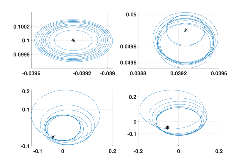
Figure 1: Uncertainty bound $\mathcal{D}(x)$ estimation at query points with successive intersection of ellipses obtained from measured data. Star ($\star$) denotes the true value of $d(x)$, lying in the intersection.

Let the time indices during exploration phase be denoted by $j$.

Fig. 1 shows the sets $E^{d}({x})$ at four fixed query points ${x}_{j}=\{[-1,2]^{\top},[1,1]^{\top},[-1,1]^{\top},[-2,-1]^{\top}\}$ as data is collected until instant $j$. This can be obtained from feasibility of (3) (with $k=j$). As $j$ increases, $E^{d}(x)$ for each $x$ is contained in the successive intersections of ellipsoids, from (6). The intersection shrinks for all points, as claimed in Proposition 2. This is seen in Fig. 1, which indicates improved information of $\mathcal{D}(x)$ with added data, for all $x\in\mathcal{X}$. At $j_{\mathrm{max}}=30$, a nonempty $\mathcal{X}_{N}$ is obtained, shown in Fig. 2. This is when we start control and set $t=0$.

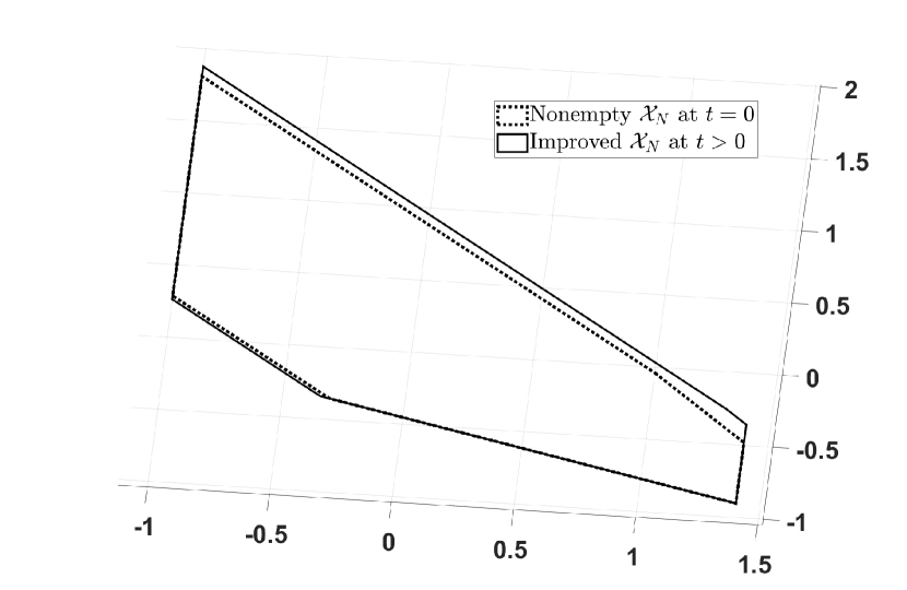
Figure 2: Terminal set construction. The set grows as estimation of $d(x)$ is improved from measurements.

V-B Robust Constraint Satisfaction

If the MPC problem (15) is feasible for parameters defined in (18), it ensures robust satisfaction of constraints in (18) for all times $t>0$. This is highlighted with a realized trajectory in Fig. 3. Furthermore, the terminal set is recomputed and improved at a $t>0$ with (14), having refined $\mathcal{P}^{d}(\mathcal{X})$ estimation from (3) (with $k=t+N$). The set grows, as seen in Fig. 2, resulting in lesser conservatism of (15).

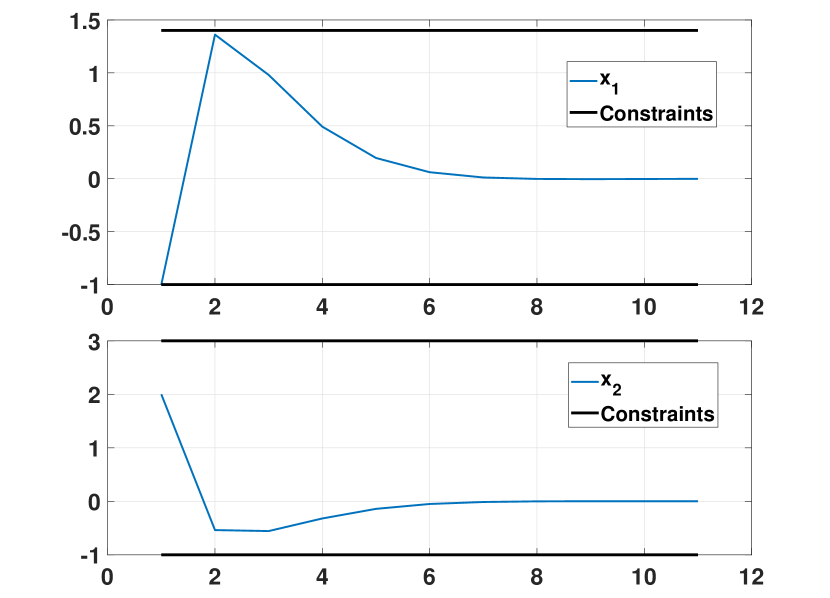
Figure 3: State trajectory with robust constraint satisfaction.

VI Conclusions

We proposed an Adaptive MPC framework to achieve robust satisfaction of state and input constraints for uncertain linear systems. The system uncertainty is assumed state dependent and globally Lipschitz. An envelope containing the uncertainty range is constructed with Quadratic Constraints (QCs), and is refined with data as the system explores the state-space. Upon collection of sufficient data, the system is able to solve a robust MPC problem for all times from a given initial state. The algorithm further reduces its conservatism by incorporating online model adaptation during control.

Appendix

Proof of Proposition 2

Let $x_{i}$ be the measurements collected at any time instant $i<t$. From (6) we see that for any given time $t$, the uncertainty domain $\mathcal{D}(\tilde{x}_{t})$ is obtained from successive intersection operations of sampled range sets at $\tilde{x}_{t}$, for all times until $t$. Hence, $\mathcal{D}(\tilde{x}_{t_{2}})=(\bigcap_{i=0}^{t_{1}}\mathcal{S}(x_{i},\tilde{x}_{t_{1}}))\bigcap_{i=t_{1}}^{t_{2}}\mathcal{S}(x_{i},\tilde{x}_{t_{2}})=\mathcal{D}(\tilde{x}_{t_{1}})\bigcap_{i=t_{1}}^{t_{2}}\mathcal{S}(x_{i},\tilde{x}_{t_{2}})$, implying $\mathcal{D}(\tilde{x}_{t_{2}})\subseteq\mathcal{D}(\tilde{x}_{t_{1}})$.

Proof of Proposition 3

Consider any vector $[x^{\top}d^{\top}1]^{\top}\in\mathbb{R}^{2n+1}$ such that $x\in E^{d}(\mathcal{X}_{k|t})$ and $[x^{\top}d^{\top}]^{\top}\in G(d)$. Given that (3) is feasible for each prediction instant $k=\{t+1,\dots,t+N\}$ at any time $t$, we multiply $[x^{\top}d^{\top}1]^{\top}$ on both sides of (3)

$$-\rho^{k}_{t}\begin{bmatrix}x\\ 1\end{bmatrix}^{\top}\bar{P}^{x}_{k|t}\begin{bmatrix}x\\ 1\end{bmatrix}+\begin{bmatrix}d\\ 1\end{bmatrix}^{\top}\bar{P}^{d}_{k|t}\begin{bmatrix}d\\ 1\end{bmatrix}$$

$$~{}~{}~{}~{}~{}~{}~{}~{}~{}~{}~{}~{}~{}~{}~{}~{}~{}~{}~{}~{}~{}~{}~{}~{}~{}~{}~{}~{}~{}~{}-\begin{bmatrix}x\\ d\\ 1\end{bmatrix}^{\top}\sum\limits_{i=0}^{t-1}\tau^{k}_{i}Q_{L}^{d}(x_{i})\begin{bmatrix}x\\ d\\ 1\end{bmatrix}\leq 0,$$

for some $\{\rho^{k}_{t},\tau^{k}_{0},\dots,\tau^{k}_{t-1}\}\geq 0$, where $\bar{P}^{x}_{k|t}$ and $\bar{P}^{d}_{k|t}$ are defined in Section IV-A. Now using Corollary 1, (IV-A) and (12), we can infer $\begin{bmatrix}d\\ 1\end{bmatrix}^{\top}\bar{P}^{d}_{k|t}\begin{bmatrix}d\\ 1\end{bmatrix}\leq 0$.

SDP for Solving (3)

For all $k=\{t+1,\dots,t+N\}$, along MPC horizon, let us use the variable nomenclature $p(\mathcal{X}_{k|t})=-\rho^{k}_{t}q^{x}_{k|t}+\sum\limits_{i=0}^{t-1}\tau^{k}_{i}L_{d}^{2}\mathbb{I}_{n},~{}q(\mathcal{X}_{k|t})=\rho^{k}_{t}(q^{x}_{k|t})^{\top}p^{x}_{k|t}-\sum\limits_{i=0}^{t-1}\tau^{k}_{i}L_{d}^{2}x_{i},~{}r(\mathcal{X}_{k|t})=-\sum\limits_{i=0}^{t-1}\tau^{k}_{i}\mathbb{I}_{n},~{}s(\mathcal{X}_{k|t})=\sum\limits_{i=0}^{t-1}\tau^{k}_{i}d(x_{i})$, and $t(\mathcal{X}_{k|t})=\rho^{k}_{t}\Big{(}1-(p^{x}_{k|t})^{\top}q^{x}_{k|t}p^{x}_{k|t}\Big{)}-\sum\limits_{i=0}^{t-1}\tau^{k}_{i}\Big{(}-L_{d}^{2}x_{i}^{\top}x_{i}+d^{\top}(x_{i})d(x_{i})\Big{)}-1$. Finding the minimum trace ellipsoid satisfying (3) is posed as an SDP [26, Section 11.4] as:

$$\begin{array}[]{llll}\displaystyle\min_{\xi}&\textnormal{trace}((q^{d}_{k|t})^{-1})\\ \ \ \text{s.t.}&\begin{bmatrix}p(\mathcal{X}_{k|t})&\mathbf{0}&q(\mathcal{X}_{k|t})&\mathbf{0}\\ \mathbf{0}&r(\mathcal{X}_{k|t})&s(\mathcal{X}_{k|t})&-\mathbb{I}_{n}\\ q^{\top}(\mathcal{X}_{k|t})&s^{\top}(\mathcal{X}_{k|t})&t(\mathcal{X}_{k|t})&(p^{d}_{k|t})^{\top}\\ \mathbf{0}&-\mathbb{I}_{n}&p^{d}_{k|t}&-(q^{d}_{k|t})^{-1}\end{bmatrix}\preceq 0,\\ &\rho^{k}_{t}\geq 0,\tau^{k}_{i}\geq 0,~{}q^{d}_{k|t}\succ 0,\\ &\forall i=0,1,\dots,t-1,\end{array}$$

with $\xi=\{q^{d}_{k|t},p^{d}_{k|t},\rho^{k}_{t},\tau^{k}_{0},\dots,\tau^{k}_{t-1}\}$ and $\mathbf{0}\in\mathbb{R}^{n\times n}$.

References

- [1] J. Friedman, T. Hastie, and R. Tibshirani, The elements of statistical learning. Springer series in statistics New York, 2001, vol. 1, no. 10.
- [2] T. J. Hastie, “Generalized additive models,” in Statistical models in S. Routledge, 2017, pp. 249–307.
- [3] B. Recht, “A tour of reinforcement learning: The view from continuous control,” Annual Review of Control, Robotics, and Autonomous Systems, vol. 2, pp. 253–279, 2019.
- [4] U. Rosolia, X. Zhang, and F. Borrelli, “Data-driven predictive control for autonomous systems,” Annual Review of Control, Robotics, and Autonomous Systems, vol. 1, pp. 259–286, 2018.
- [5] D. P. Bertsekas and D. A. Castanon, “Adaptive aggregation methods for infinite horizon dynamic programming,” IEEE Transactions on Automatic Control, vol. 34, no. 6, pp. 589–598, 1989.
- [6] C. J. Watkins and P. Dayan, “Q-learning,” Machine learning, vol. 8, no. 3-4, pp. 279–292, 1992.
- [7] M. Krstic, I. Kanellakopoulos, and P. V. Kokotovic, Nonlinear and adaptive control design. Wiley, 1995.
- [8] S. Sastry and M. Bodson, Adaptive control: Stability, convergence and robustness. Courier Corporation, 2011.
- [9] S. Dean, S. Tu, N. Matni, and B. Recht, “Safely learning to control the constrained linear quadratic regulator,” in 2019 American Control Conference (ACC), July 2019, pp. 5582–5588.
- [10] J. C. Doyle, N. Matni, Y.-S. Wang, J. Anderson, and S. Low, “System level synthesis: A tutorial,” in 2017 IEEE 56th Annual Conference on Decision and Control (CDC). IEEE, 2017, pp. 2856–2867.
- [11] M. Tanaskovic, L. Fagiano, R. Smith, and M. Morari, “Adaptive receding horizon control for constrained MIMO systems,” Automatica, vol. 50, no. 12, pp. 3019–3029, 2014.
- [12] M. Bujarbaruah, X. Zhang, and F. Borrelli, “Adaptive MPC with chance constraints for FIR systems,” in 2018 Annual American Control Conference (ACC), June 2018, pp. 2312–2317.
- [13] M. Lorenzen, M. Cannon, and F. Allgöwer, “Robust MPC with recursive model update,” Automatica, vol. 103, pp. 461 – 471, 2019.
- [14] J. Köhler, E. Andina, R. Soloperto, M. A. Müller, and F. Allgöwer, “Linear robust adaptive model predictive control : Computational complexity and conservatism,” arXiv preprint arXiv:1909.01813, 2019.
- [15] M. Bujarbaruah, X. Zhang, M. Tanaskovic, and F. Borrelli, “Adaptive MPC under time varying uncertainty: Robust and Stochastic,” arXiv preprint arXiv:1909.13473, 2019.
- [16] L. Hewing and M. N. Zeilinger, “Cautious model predictive control using gaussian process regression,” arXiv preprint arXiv:1705.10702, 2017.
- [17] R. Soloperto, M. A. Müller, S. Trimpe, and F. Allgöwer, “Learning-based robust model predictive control with state-dependent uncertainty,” in IFAC Conference on Nonlinear Model Predictive Control, Madison, Wisconsin, USA, Aug. 2018.
- [18] T. Koller, F. Berkenkamp, M. Turchetta, and A. Krause, “Learning-based model predictive control for safe exploration,” in 2018 IEEE Conference on Decision and Control (CDC). IEEE, 2018, pp. 6059–6066.
- [19] S. H. Nair, M. Bujarbaruah, and F. Borrelli, “Modeling of dynamical systems via successive graph approximations,” arXiv preprint arXiv:1910.03719, 2019.
- [20] P. J. Goulart, E. C. Kerrigan, and J. M. Maciejowski, “Optimization over state feedback policies for robust control with constraints,” Automatica, vol. 42, no. 4, pp. 523–533, 2006.
- [21] J. Löfberg, Minimax approaches to robust model predictive control. Linköping University Electronic Press, 2003, vol. 812.
- [22] I. Kolmanovsky and E. G. Gilbert, “Theory and computation of disturbance invariant sets for discrete-time linear systems,” Mathematical Problems in Engineering, vol. 4, no. 4, pp. 317–367, 1998.
- [23] F. Borrelli, A. Bemporad, and M. Morari, Predictive control for linear and hybrid systems. Cambridge University Press, 2017.
- [24] B. Kouvaritakis and M. Cannon, Model predictive control: Classical, robust and stochastic. Springer, 2016.
- [25] F. Blanchini, “Set invariance in control,” Automatica, vol. 35, no. 11, pp. 1747–1767, 1999.
- [26] G. C. Calafiore and L. El Ghaoui, Optimization models. Cambridge university press, 2014.