A coarse-grained phase-field crystal model of plastic motion

Abstract

The phase-field crystal model in an amplitude equation approximation is shown to provide an accurate description of the deformation field in defected crystalline structures, as well as of dislocation motion. We analyze in detail stress regularization at a dislocation core given by the model, and show how the Burgers vector density can be directly computed from the topological singularities of the phase-field amplitudes. Distortions arising from these amplitudes are then supplemented with non-singular displacements to enforce mechanical equilibrium. This allows for a consistent separation of plastic and elastic time scales in this framework. A finite element method is introduced to solve the combined amplitude and elasticity equations, which is applied to a few prototypical configurations in two spatial dimensions for a crystal of triangular lattice symmetry: i) the stress field induced by an edge dislocation with an analysis of how the amplitude equation regularizes stresses near the dislocation core, ii) the motion of a dislocation dipole as a result of its internal interaction, and iii) the shrinkage of a rotated grain. We compare our results with those given by other extensions of classical elasticity theory, such as strain-gradient elasticity and methods based on the smoothing of Burgers vector densities near defect cores.

1 Introduction

The distribution of dislocations and grain boundaries and their motion play an important role in materials physics as they determine many material properties and response, especially in polycrystalline and heteroepitaxial systems. A great deal of research has been devoted to the study of such systems to better understand the interplay between the many disparate length scales involved (Rollett et al., 2015, Sethna et al., 2017). Microscopic theories, such as Density Functional Theory and Molecular Dynamics, provide detailed descriptions at the microscopic scale, but are unfortunately restricted to relatively small length and time scales. Coarse-grained methods have also been introduced, such as Discrete Dislocation Dynamics (DDD) (Kubin and Canova, 1992, Devincre et al., 1992), which evolve dislocation lines through Peach-Koehler type forces. These methods can examine mechanical properties on large length and time scales while treating dislocations explicitly. However, they rely on the phenomenology involved in dislocation line mobilities and their reconnections. Phase-field (PF) models also belong to the class of coarse-grained approaches. They are based on the description of distinct phases via continuous order parameters, and the implicit description of interfaces between them. Early work on the application of PF models to the description of extended defects and, in turn, to their motion, focused on describing elementary defects as an eigenstrain, which is then mapped onto a set of phase fields (Wang et al., 2001, Koslowski et al., 2002, Rodney et al., 2003, Bulatov and Cai, 2006, Wang and Li, 2010). As discussed extensively in Wang and Li (2010), a fundamental advantage of this methodology is that physical parameters describing dislocation energies are subsumed in the energy model, and hence do not need separate specification (e.g, generalized stacking fault energies). The evolution of the phase fields is purely dissipative, and is driven by minimization of a phenomenological energy of the Ginzburg-Landau type. However, a few quantities that remain central to the analysis of defect motion still require a priori specification, such as active slip systems and defect mobilities. As we will argue below, the phase field crystal (PFC) model overcomes these limitations.

The PFC model (Elder et al., 2002, Elder and Grant, 2004, Emmerich et al., 2012) is based on the definition of a continuous order parameter or field $\psi$ that is related to the atomic number density. A free energy functional is introduced that is minimized by a periodic field with the desired lattice symmetry. The temporal evolution of $\psi$ is assumed to be governed by conserved and dissipative dynamics, hence changing on effectively diffusive time scales. The formulation is akin to Classical Density Functional Theory, and it has been justified to some extent on those grounds as well (Elder et al., 2007, van Teeffelen et al., 2009, Archer et al., 2019). Therefore this modeling is intermediate between fully atomistic and classical continuum theories. Diffusive time scales and atomistic length scales allow for describing grain boundaries in detail, their motion, and the response of complex polycrystalline configurations, as these phenomena are well described by energy relaxation alone, without requiring the calculation of any stress fields in the grains (Li et al., 2018, Wu and Voorhees, 2009, Backofen et al., 2014, Mianroodi and Svendsen, 2015, Hirvonen et al., 2016, Clayton and Knap, 2016, Köhler et al., 2016). By focusing on the complex slowly-varying amplitudes of $\psi$, a spatial coarse-grained version of the PFC model has been introduced (Goldenfeld et al., 2005, Athreya et al., 2006, Goldenfeld et al., 2006, Yeon et al., 2010). This amplitude expansion (APFC) approach provides an approximate description of the atomic length scale (Spatschek and Karma, 2010, Elder et al., 2010, Heinonen et al., 2014, Salvalaglio et al., 2019). Due to its coarse grained nature and the use of adaptive numerical methods, computational costs can be drastically reduced and systems that are orders of magnitude larger than those accessible with PFC models can be described with APFC models (Praetorius et al., 2019). A different methodology but analogous in many respects is the Field Theory of Dislocation motion (Acharya, 2001, Zhang et al., 2015, 2018), and its more recent nanoscale implementation in the Generalized Disclination Theory (Zhang and Acharya, 2018).

At variance with models explicitly tracking defects and grain boundaries, the (A)PFC model starts from the specification of the governing free energy from which lattice symmetry, possible defects, and their combination rules, follow. Despite these advantages, a long-standing difficulty associated with the (A)PFC model is that the evolution of the field is diffusive, hence elastic response in the time scale appropriate for plastic motion is incomplete. The first attempt to overcome this problem was the development of the so-called modified PFC (MPFC) model given in (Stefanovic et al., 2006), in which a higher-order time derivative was introduced into the equation of motion. While this approach does lead to faster elastic relaxation, it gives incorrect behavior in the large wavelength limit, as pointed out in Majaniemi and Grant (2007) and Heinonen et al. (2016). More recently, a complete transport theory has been developed in which the order parameter that enters the PFC model is included as a constitutive component within the more general laws of balance of mass and momentum (Heinonen et al., 2016). While these models do introduce a “fast” time scale on the order of the speed of sound, they can become computationally expensive when the time scale of mechanical relaxation is orders of magnitude faster than the time scales for mass diffusion and plastic distortion. An alternative and computationally convenient method seeks to enforce elastic equilibrium through an interpolation scheme in the PFC model designed to achieve fast mechanical relaxation (Zhou et al., 2019b). The method, however, is limited to uniaxial external deformation. Yet another approach in the APFC model (Heinonen et al., 2014) recognizes that the phases of the complex amplitudes contain information about the elastic distortion and that instantaneous mechanical equilibrium can be achieved by relaxing these fields at a faster rate. Similar to other approaches, this limits the computational efficiency of the method and lacks transparency. A more recent approach that retains the atomic density as constitutively governing plastic slip but adds the elastic distortion caused by lattice incompatibility was described in Skaugen et al. (2018a, b). This latter approach is also computationally efficient, and provides for the connection between the phase field and elasticity theory in the presence of dislocations. We will extend this latter approach to the APFC model in order to provide a computational approach that is suitable for larger systems and spatial scales.

In this work, we thus present a coarse-grained description of deformations in crystals and plasticity based on the APFC model, intermediate between atomistic and continuum length scales. Section 2 summarizes the equations governing the evolution of the PFC model and the associated description based on the slowly varying complex amplitudes, i.e., on the APFC model. While the expansion in a slowly varying amplitude assumes prior knowledge of the lattice symmetry, the latter simply follows from the minimization of the free energy functional defining the system of interest. This description is advantageous from a computational point of view as it does not need to resolve the variation of the order parameter at the scale of the underlying lattice parameter as in the PFC model. It is limited, however, to small distortions away from a reference lattice, not an uncommon restriction in this class of studies, as it focuses on length scales larger than the atomic spacing. Section 3 addresses how, in the APFC model, stress fields in the presence of defects are calculated, and how mechanical equilibrium is enforced on the time scale of defect motion. A finite element implementation of the combined system of equations is provided in Sec. 4, followed by our numerical results in Sec. 5. We begin by studying the stress field created by an isolated, stationary dislocation in a two-dimensional, large crystal (Sec. 5.1). The computed stress agrees with classical elasticity far from the defect core, and also with results provided by either first strain gradient elasticity (Lazar and Maugin, 2005), or Burgers vector smoothing methods (Cai et al., 2006) near the core. Sections 5.2 and 5.3 present our results on dislocation dipoles and their motion under each other’s influence. Sec. 5.4 addresses the study of grain shrinkage along with the analysis of defect distribution achieved within the presented framework.

2 Amplitude Phase-Field Crystal (APFC) model

The PFC model describes a crystal lattice by means of a continuous, periodic field $\psi$, the dimensionless atomic probability density difference (Elder et al., 2002, Elder and Grant, 2004, Emmerich et al., 2012). A phenomenological free energy is introduced as

$$F_{\psi}=\int_{\Omega}\left[\frac{\Delta B_{0}}{2}\psi^{2}+\frac{B^{x}_{0}}{2}\psi(1+\nabla^{2})^{2}\psi-\frac{t}{3}\psi^{3}+\frac{v}{4}\psi^{4}\right]d\mathbf{r},$$ (1)

which describes a first order transition between a disordered/liquid phase, where $\psi$ is uniform, and an ordered/crystalline phase, where $\psi$ is periodic in the domain $\Omega$. $\Delta B_{0}$, $B_{0}^{x}$, $v$ and $t$ are parameters determining which phase minimizes the free energy $F_{\psi}$ (Elder et al., 2007). In the standard approach, the evolution towards equilibrium for out-of-equilibrium configurations is described by the gradient flow ensuring conservation of $\psi$

$$\frac{\partial\psi}{\partial t}=M\nabla^{2}\frac{\delta F_{\psi}}{\delta\psi},$$ (2)

where $M$ is a mobility. In the crystalline state, $\psi$ can be generally approximated as a sum of plane waves, i.e.,

$$\psi=\psi_{0}+\sum_{\mathbf{q}}A_{\mathbf{q}}e^{i\mathbf{q}\cdot\mathbf{r}}=\psi_{0}+\sum_{j}^{N}A_{j}e^{i\mathbf{q}_{j}\cdot\mathbf{r}}+{\rm c.c.},$$ (3)

where $\psi_{0}$ is the average density, set to zero in the following, $A_{j}$ are the (complex) fields corresponding to the amplitudes of each plane wave and $\{\mathbf{q}_{j}\}$ is the set of $N$ reciprocal lattice vectors representing a specific crystal symmetry.

In the so-called amplitude expansion of the PFC model (APFC) (Goldenfeld et al., 2005, Athreya et al., 2006, Goldenfeld et al., 2006), the crystal structure is described directly by means of $A_{j}$. They account for distortions and rotations of the crystal structure with respect to a reference state accounted for by a proper set of $\mathbf{q}_{j}$ vectors. Under the assumption of slowly varying amplitudes, the free energy of the system expressed in terms of $A_{j}$ reads

$$F_{A}=\int_{\Omega}\bigg{[}\frac{\Delta B_{0}}{2}\Phi+\frac{3v}{4}\Phi^{2}+\sum_{j=1}^{N}\left(B_{0}^{x}|\mathcal{G}_{j}A_{j}|^{2}-\frac{3v}{2}|A_{j}|^{4}\right)+f^{\rm s}(\{A_{j}\},\{A^{*}_{j}\})\bigg{]}d\mathbf{r},$$ (4)

where $\mathcal{G}_{j}=\nabla^{2}+2i\mathbf{q}_{j}\cdot\nabla$ and $\Phi=2\sum_{j=1}^{N}|A_{j}|^{2}$. The term $f^{\rm s}(\{A_{j}\},\{A_{j}^{*}\})$ corresponds to a complex polynomial of $A_{j}$ and $A_{j}^{*}$ and is determined by the crystalline symmetry of the reference lattice (Elder et al., 2010, Salvalaglio et al., 2017). Amplitude functions allow for a full description of elastic deformation within the PFC framework, and the associated energy in Eq. (4) contains the elastic energy associated with deformations (Elder et al., 2010, Heinonen et al., 2014). The evolution equation of the $A_{j}$’s can be derived from Eq. (2), and reads

$$\frac{\partial A_{j}}{\partial t}=-|\mathbf{q}_{j}|^{2}\frac{\delta F_{A}}{\delta A_{j}^{*}},$$ (5)

with time rescaled by $M$. In this work we focus on two-dimensional crystals with triangular symmetry ($N=3$) described by

$$\begin{gathered}\mathbf{q}_{1}=k_{0}\left(-\sqrt{3}/2,-1/2\right),\ \ \mathbf{q}_{2}=k_{0}(0,1),\ \ \mathbf{q}_{3}=k_{0}\left(\sqrt{3}/2,-1/2\right),\end{gathered}$$ (6)

with $k_{0}=1$, while $f^{\rm s}(\{A_{j}\},\{A_{j}^{*}\})=-2t(A_{1}A_{2}A_{3}+A_{1}^{*}A_{2}^{*}A_{3}^{*})$.

3 APFC dynamics and mechanical equilibrium

Following Skaugen et al. (2018a, b), we aim at computing the density field $\psi$ so that it remains in elastic equilibrium at all times in the presence of mobile dislocations. Besides solving Eq. (2) this requires computing an additional smooth distortion $\mathbf{u}^{\delta}$ to fulfill mechanical equilibrium, i.e., $\nabla\cdot\boldsymbol{\sigma}=0$ with $\boldsymbol{\sigma}$ the total stress field. In the PFC approach, $\psi(\mathbf{r},t)$ is then replaced by $\psi(\mathbf{r}-\mathbf{u}^{\delta},t)$ (Skaugen et al., 2018a). In the APFC approach we only have access to the amplitudes by solving Eq. (5) from which $\psi$ can be reconstructed. For small displacement $\mathbf{u}^{\delta}$ we can write

$$\begin{split}\psi^{\prime}(\mathbf{r}-\mathbf{u}^{\delta},t)&\stackrel{{\scriptstyle\mathbf{u}^{\delta}\rightarrow 0}}{{=}}\psi(\mathbf{r},t)-[\nabla\psi(\mathbf{r},t)]^{\rm T}\cdot\mathbf{u}^{\delta}+\mathcal{E}(||\mathbf{u}^{\delta}||^{2})\\ &=\sum_{\mathbf{q}}\left\{A_{\mathbf{q}}(\mathbf{r},t)-[\nabla A_{\mathbf{q}}(\mathbf{r},t)]^{\rm T}\cdot\mathbf{u}^{\delta}-i\mathbf{q}\cdot\mathbf{u}^{\delta}A_{\mathbf{q}}(\mathbf{r},t)\right\}e^{i\mathbf{q}\cdot\mathbf{r}}+\mathcal{E}(||\mathbf{u}^{\delta}||^{2})\\ &=\sum_{\mathbf{q}}A_{\mathbf{q}}^{\prime}(\mathbf{r},\mathbf{u}^{\delta},t)e^{i\mathbf{q}\cdot\mathbf{r}}+\mathcal{E}(||\mathbf{u}^{\delta}||^{2}),\end{split}$$ (7)

with

$$A_{\mathbf{q}}^{\prime}(\mathbf{r},\mathbf{u}^{\delta},t)=(1-i\mathbf{q}\cdot\mathbf{u}^{\delta})A_{\mathbf{q}}(\mathbf{r},t)-[\nabla A_{\mathbf{q}}(\mathbf{r},t)]^{\rm T}\cdot\mathbf{u}^{\delta},$$ (8)

which are the amplitudes modified by the deformation $\mathbf{u}^{\delta}$ and need to be computed. Under the assumption of slowly varying amplitudes, as required by the APFC approach, this quantity is simply given by (Spatschek and Karma, 2010)

$$A_{\mathbf{q}}^{\prime}(\mathbf{r},\mathbf{u}^{\delta},t)=A_{\mathbf{q}}(\mathbf{r},t)e^{-i\mathbf{q}\cdot\mathbf{u}^{\delta}},$$ (9)

as

$$A_{\mathbf{q}}(\mathbf{r},t)e^{-i\mathbf{q}\cdot\mathbf{u}^{\delta}}=A_{\mathbf{q}}(\mathbf{r},t)[\cos(\mathbf{q}\cdot\mathbf{u}^{\delta})-i\sin(\mathbf{q}\cdot\mathbf{u}^{\delta})]\stackrel{{\scriptstyle\mathbf{u}^{\delta}\rightarrow 0}}{{\approx}}(1-i\mathbf{q}\cdot\mathbf{u}^{\delta})A_{\mathbf{q}}(\mathbf{r},t),$$ (10)

where the last expression corresponds to Eq. (8) for negligible gradients of amplitudes. In the following we will use Eq. (9). A comparison with approximations in Eq. (8) and (10) will be given in Sect. 5.4.

As shown in (Skaugen et al., 2018a), $\mathbf{u}^{\delta}$ can be determined through a Helmholtz decomposition into curl- and divergence-free parts,

$$u_{i}^{\delta}=\partial_{i}\varphi+\epsilon_{ij}\partial_{j}\alpha,$$ (11)

with $\varphi$ and $\alpha$ to be determined. $\varphi$ can be computed from a smooth strain $\varepsilon_{ij}^{\delta}$ as

$$\nabla^{2}\varphi=\rm{Tr}(\boldsymbol{\varepsilon}^{\delta}).$$ (12)

The same holds for $\alpha$ and read

$$\nabla^{4}\alpha=-2\epsilon_{ij}\partial_{ik}\varepsilon_{jk}^{\delta}.$$ (13)

The strain field $\varepsilon_{ij}^{\delta}$ is compatible, and the corresponding stress can be computed from the difference between the total stress, $\boldsymbol{\sigma}$, and a stress computed from the amplitude functions, $\sigma_{ij}^{\psi}$, as (Skaugen et al., 2018b)

$$\sigma^{\delta}_{ij}=\sigma_{ij}-\sigma^{\psi}_{ij}=\epsilon_{ik}\epsilon_{jl}\partial_{kl}\chi-\sigma_{ij}^{\psi},$$ (14)

where $\chi$ is the Airy stress function. Exploiting the formulation reported in Skaugen et al. (2018b), the stress $\sigma_{ij}^{\psi}$ can be obtained by

$$\sigma_{ij}^{\psi}=\langle\sigma_{ij}\rangle=\langle(\partial_{i}\mathcal{L}\psi)\partial_{j}\psi-\mathcal{L}\psi\partial_{ij}\psi\rangle,$$ (15)

where $\mathcal{L}\equiv 1+\nabla^{2}$ and $\langle\cdots\rangle$ the average over the unit cell, here necessary to compute $\sigma_{ij}^{\psi}$ in terms of $A_{j}$. Using Eq. (3) and by integrating over the unit cell we obtain

$$\sigma_{ij}^{\psi}=\sum_{\mathbf{q}}\left\{[(\partial_{i}+iq_{i})(\nabla^{2}+2i\mathbf{q}\cdot\nabla)A_{\mathbf{q}}][(\partial_{j}-iq_{j})A_{\mathbf{-q}}]-[(\nabla^{2}+2i\mathbf{q}\cdot\nabla)A_{\mathbf{q}}][(\partial_{i}-iq_{i})(\partial_{j}-iq_{j})A_{\mathbf{-q}}]\right\}.$$ (16)

In Eq. (14) $\chi$ is given by

$$(1-\kappa)\nabla^{4}\chi=2\mu\epsilon_{ij}\partial_{i}B_{j}(\mathbf{r})=(\epsilon_{ik}\epsilon_{jl}\partial_{ij}\sigma_{kl}^{\psi}-\kappa\nabla^{2}\sigma_{kk}^{\psi}),$$ (17)

with $\mathbf{B}(\mathbf{r})$ the Burgers vector density, and $\kappa=\lambda/(2(\lambda+\mu))$, with $\lambda$ and $\mu$ the two Lamé coefficients. Once $\sigma_{ij}^{\delta}$ is computed, the smooth strain to be used in Eqs. (12) and (13) is obtained by

$$\varepsilon_{ij}^{\delta}=\frac{1}{2\mu}(\sigma_{ij}^{\delta}-\nu\delta_{ij}\mathrm{Tr}(\boldsymbol{\sigma}^{\delta})),$$ (18)

and, in turn, the smooth deformation $\mathbf{u}^{\delta}$ is determined from Eqs. (11)–(13). Once $\mathbf{u}^{\delta}$ is known, Eq. (9) can be used to update the amplitudes.

We note that, in our formulation, although the stress $\sigma_{ij}$ is required to satisfy mechanical equilibrium at each time step, the configuration of the system changes as dislocations move in time. Dislocation motion and net plastic flow follow from the dissipative evolution of the phase field. The separation of time scales between dissipative plastic motion and elastic relaxation is a basic assumption in most modeling approaches, such as, for instance, discrete dislocation dynamics (Kubin and Canova, 1992, Devincre et al., 1992). The strain rate dependence of plastic deformation can then be still maintained in the modeling with instantaneous elastic equilibrium, as demonstrated in e.g., recent PFC study of mechanical deformation of graphene grain boundaries (Zhou et al., 2019a).

4 Finite element implementation

The implementation of the system of partial differential equations (PDEs) reported in Sect. 3 builds on the discretization of the standard APFC model described in Salvalaglio et al. (2017), Praetorius et al. (2019) and extends it to maintain mechanical equilibrium. It is based on the adaptive FEM toolbox AMDiS (Vey and Voigt, 2007, Witkowski et al., 2015). The governing equations are solved as systems of second-order PDEs with semi-implicit integration schemes. For the sake of clarity, these integration schemes are reported in the following in matrix form $\mathbf{L}\cdot\mathbf{x}=\mathbf{R}$, with $\mathbf{x}$ the vector of unknowns. We define an auxiliary complex field $B_{j}=(\nabla^{2}+2i\mathbf{q}^{n}\cdot\nabla)A_{j}=\mathcal{G}_{j}A_{j}$ and explicitly consider the real and imaginary part of $A_{j}$ and $B_{j}$ such as $A_{j}=A_{{\rm R},j}+iA_{{\rm I},j}$ and $B_{j}=B_{{\rm R},j}+iB_{{\rm I},j}$. The following system of equations is then used for numerically integrating the evolution equation (5) for the amplitude $A_{j}$

$$\mathbf{L}=\begin{bmatrix}-\nabla^{2}&\mathcal{P}&1&0\\[7.5pt] -\mathcal{P}&-\nabla^{2}&0&1\\[7.5pt] G_{1}(\{A_{i}^{(n)}\})&0&K\nabla^{2}&-K\mathcal{P}\\[7.5pt] 0&G_{2}(\{A_{i}^{(n)}\})&K\mathcal{P}&K\nabla^{2}\end{bmatrix}\qquad\mathbf{x}=\begin{bmatrix}A_{{\rm R},j}^{(n+1)}\\[7.5pt] A_{{\rm I},j}^{(n+1)}\\[7.5pt] B_{{\rm R},j}^{(n+1)}\\[7.5pt] B_{{\rm I},j}^{(n+1)}\end{bmatrix}\qquad\mathbf{R}=\begin{bmatrix}0\\[7.5pt] 0\\[7.5pt] H_{1}(\{A_{i}^{(n)}\})\\[7.5pt] H_{2}(\{A_{i}^{(n)}\})\\ \end{bmatrix}$$ (19)

where $n$ is the time step index, $\tau_{n}>0$ is the time step size at step $n$, $\mathcal{P}=2\mathbf{q}_{j}\cdot\nabla$, $K=|\mathbf{q}_{j}|^{2}B_{0}^{x}$, and

$$\begin{split}G_{1}(\{A_{i}\})=&\dfrac{1}{\tau_{n}}+|\mathbf{q}_{j}|^{2}\Delta B+3v|\mathbf{q}_{j}|^{2}\left(\Phi+A_{{\rm R},j}^{2}-A_{{\rm I},j}^{2}\right),\\ G_{2}(\{A_{i}\})=&\dfrac{1}{\tau_{n}}+|\mathbf{q}_{j}|^{2}\Delta B+3v|\mathbf{q}_{j}|^{2}\left(\Phi+A_{{\rm I},j}^{2}-A_{{\rm R},j}^{2}\right),\\ H_{1}(\{A_{i}\})=&\left[\dfrac{1}{\tau_{n}}+6|\mathbf{q}_{j}|^{2}vA_{{\rm R},j}^{2}\right]A_{{\rm R},j}-|\mathbf{q}_{j}|^{2}\text{Re}\left(\frac{\delta f^{\rm tri}}{\delta A_{j}^{*}}\right),\\ H_{2}(\{A_{i}\})=&\left[\dfrac{1}{\tau_{n}}+6|\mathbf{q}_{j}|^{2}vA_{{\rm I},j}^{2}\right]A_{{\rm I},j}-|\mathbf{q}_{j}|^{2}\text{Im}\left(\frac{\delta f^{\rm tri}}{\delta A_{j}^{*}}\right).\end{split}$$ (20)

$\{A_{i}\}$ refers to the entire set of amplitudes $A_{i}$ with $i=1,...,N$ as they enter $\Phi$ and $f^{\rm tri}$. Exploiting the definition of $B_{j}$ reported above, the components of the stress $\boldsymbol{\sigma}^{\psi}$ can be written as

$$\begin{split}\sigma_{lm}^{\psi}=&\left\{[(\partial_{l}+iq_{l})B_{j}][(\partial_{m}-iq_{m})A_{j}^{*}]-B_{j}[(\partial_{l}-iq_{l})(\partial_{m}-iq_{m})A_{j}^{*}]+{\rm c.c.}\right\}\\ =2&\left[\partial_{l}B_{{\rm R},j}\partial_{m}A_{{\rm R},j}+\partial_{l}B_{{\rm I},j}\partial_{m}A_{{\rm I},j}+2q^{j}_{l}B_{{\rm R},j}\partial_{m}A_{{\rm I},j}-2q^{j}_{l}B_{{\rm I},j}\partial_{m}A_{{\rm R},j}-q^{j}_{m}A_{{\rm I},j}\partial_{l}B_{{\rm R},j}+q^{j}_{m}A_{{\rm R},j}\partial_{l}B_{{\rm I},j}\right.\\ &\left.+2q^{j}_{l}q^{j}_{m}A_{{\rm R},j}B_{{\rm R},j}+2q^{j}_{l}q^{j}_{m}A_{{\rm I},j}B_{{\rm I},j}-B_{{\rm R},j}\partial_{lm}A_{{\rm R},j}-B_{{\rm I},j}\partial_{lm}A_{{\rm I},j}+q^{j}_{m}B_{{\rm R},j}\partial_{l}A_{{\rm I},j}-q^{j}_{m}B_{{\rm I},j}\partial_{l}A_{{\rm R},j}\right]\end{split}$$ (21)

where the real and imaginary parts of $A_{j}$ and $B_{j}$ have been considered. Note that Eq. (21) contains the variables numerically computed by the system in Eq. (19), along with their first and second derivatives. Therefore, the stress can be determined directly from the results of the evolution equations at every time step, without explicitly computing the third-order equation (16). The semi-implicit integration scheme used to solve the fourth-order PDE in Eq. (17) for $\chi$ reads

$$\mathbf{L}=\begin{bmatrix}\nabla^{2}&-1\\[6.49994pt] 0&(1-\kappa)\nabla^{2}\end{bmatrix},\quad\mathbf{x}=\begin{bmatrix}\chi\\[7.5pt] \eta\end{bmatrix},\quad\mathbf{R}=\begin{bmatrix}0\\[7.5pt] \mathcal{Q}-\kappa\nabla^{2}\sigma_{ii}^{\psi}\end{bmatrix},$$ (22)

where

$$\mathcal{Q}=\epsilon_{ik}\epsilon_{jl}\partial_{ij}\sigma_{kl}^{\psi}\stackrel{{\scriptstyle 2D}}{{=}}\partial_{xx}\sigma_{yy}^{\psi}+\partial_{yy}\sigma_{xx}^{\psi}-\partial_{xy}\sigma_{yx}^{\psi}-\partial_{yx}\sigma_{xy}^{\psi},$$ (23)

and $\eta$ an auxiliary variable such as $\eta=\nabla^{2}\chi$. The FEM calculation for $\chi$ is also exploited to compute the second derivatives of this field to be used in Eq. (14) (additional auxiliary variables $\xi_{ij}$ such as $\xi_{ij}=\partial_{ij}\chi$ may be added to the system Eq. (23)). In turn, $\varepsilon_{ij}^{\delta}$ can be computed straightforwardly from Eqs. (18). $\varphi$ and $\alpha$ can then be determined from $\varepsilon_{ij}^{\delta}$. The semi-implicit integration scheme used to solve the fourth-order PDE in Eq. (13) yielding $\alpha$ reads

$$\mathbf{L}=\begin{bmatrix}\nabla^{2}&-1\\[6.49994pt] 0&\nabla^{2}\par\end{bmatrix},\quad\mathbf{x}=\begin{bmatrix}\alpha\\[7.5pt] \zeta\end{bmatrix},\quad\mathbf{R}=\begin{bmatrix}0\\[7.5pt] \mathcal{S}\end{bmatrix},$$ (24)

where

$$\mathcal{S}=-2\epsilon_{ij}\partial_{ik}\varepsilon_{jk}^{\delta}\stackrel{{\scriptstyle 2D}}{{=}}-2\partial_{xx}\varepsilon_{yx}^{\delta}-2\partial_{xy}\varepsilon_{yy}^{\delta}+2\partial_{yx}\varepsilon_{xx}^{\delta}+2\partial_{yy}\varepsilon_{xy}^{\delta},$$ (25)

and $\zeta$ an auxiliary variable such as $\zeta=\nabla^{2}\alpha$. The Poisson equation for $\varphi$ is straightforwardly implemented as a single second-order equation (12). With values of $\alpha$ and $\varphi$, $\mathbf{u}^{\delta}$ can then be computed from Eq. (11) and the amplitudes updated as reported in Sect. 3, namely by Eq. (9). Vanishing potentials at the boundaries are ensured by Dirichlet boundary conditions, while both periodic boundary conditions and no-flux Neumann boundary conditions can be used for amplitudes equations as the systems considered here have constant values for $A_{j}$ at the boundaries. In the FEM framework, quadratic basis function are used to allow for explicit evaluation of first- and second-order derivatives when needed. Numerical solutions reported below are performed with time steps in the range of $\tau_{n}=0.1,\ldots,1$, by using spatial mesh adaptivity (see Salvalaglio et al. (2017), Praetorius et al. (2019) for more information).

More general boundary conditions can be implemented in this APFC approach. Traction boundary conditions have been introduced earlier in the PFC model for the study of mechanical deformation through an extra free energy penalty term proportional to $(\psi-\psi_{\rm trac})^{2}$, where $\psi_{\rm trac}$ is the fixed PFC density imposed on several atomic layers at the boundaries (Berry et al., 2006, Stefanovic et al., 2009, Adland et al., 2013). This extra term can be used to, e.g., apply a constant shear (Berry et al., 2006, Adland et al., 2013) or uniaxial tensile load (Stefanovic et al., 2009). It would be straightforward to adopt a similar procedure on the APFC by imposing an energy penalty in terms of complex amplitudes. On the other hand, general scenarios of traction boundary conditions are straightforward to implement in this approach as we work directly with the stress field. Specific values of tractions $\mathbf{T}=\boldsymbol{\sigma}\cdot\hat{\mathbf{n}}$ (where $\hat{\mathbf{n}}$ is the boundary surface normal) can be imposed as boundary conditions on the Airy stress function $\chi$ governed by Eq. (17), given that $T_{i}=\sigma_{ij}\hat{n}_{j}=(\epsilon_{ik}\epsilon_{jl}\partial_{kl}\chi)\hat{n}_{j}$.

5 Numerical results

5.1 Single Dislocation in a finite crystal

We first consider a configuration that includes a single dislocation. The amplitudes are initialized by considering the displacement field given by an edge dislocation with Burgers vector parallel to the $x$-direction, i.e., $\mathbf{b}=(b_{x},0)$ with $b_{x}=a=4\pi/\sqrt{3}$ and $a$ the lattice spacing. Amplitudes are set by (Spatschek and Karma, 2010, Salvalaglio et al., 2017)

$$A_{j}=\phi\exp\left(i\mathbf{q}_{j}\cdot\mathbf{u}\right),$$ (26)

where $\phi$ is the real value of amplitudes for a relaxed and unrotated crystal that can be determined through free energy minimization by assuming constant and real amplitudes (Elder et al., 2010, Salvalaglio et al., 2017), and $\mathbf{u}$ the displacement field. The components of $\mathbf{u}$ for an edge dislocation are given by (Anderson et al., 2017)

$$\begin{split}u_{x}&=\frac{b}{2\pi}\left[\arctan{\left(\frac{y}{x}\right)}+\frac{xy}{2(1-\nu)(x^{2}+y^{2})}\right],\\ u_{y}&=-\frac{b}{2\pi}\left[\frac{(1-2\nu)}{4(1-\nu)}\log{\left(x^{2}+y^{2}\right)}+\frac{x^{2}-y^{2}}{4(1-\nu)(x^{2}+y^{2})}\right],\\ \end{split}$$ (27)

with $\nu$ the Poisson’s ratio. Since the displacement field components in Eq. (27) are singular at the origin, corresponding to the nominal position of the dislocation core (Anderson et al., 2017), a local smoothing of the initial condition is introduced. The elastic energy of a single dislocation in bulk, namely in an ideally infinite crystal, is not finite in two dimensions. Therefore, we embed the amplitudes obtained by Eqs. (26) and (27) in a circular grain with radius $R$ surrounded by a disordered (liquid) phase. In practice, for $r=\sqrt{x^{2}+y^{2}}>R$ both the real and the imaginary parts of the amplitudes are set to zero. The parameters of the (A)PFC free energy are set as $B_{x}=0.98$, $v=1/3$, $t=1/2$ and, to allow for the coexistence of the solid and liquid phases, $\Delta B_{0}\lesssim 8t^{2}/(135v)$. Having a single dislocation in the system shifts the free energy of the solid to a slightly higher value; thus $\Delta B_{0}$ should be slightly smaller than that of the ideal, dislocation-free case. Still, we have verified that a negligible growth velocity of the grain is observed for $\Delta B_{0}=0.042$ over the timescale of interest (i.e., during the relaxation of the system).

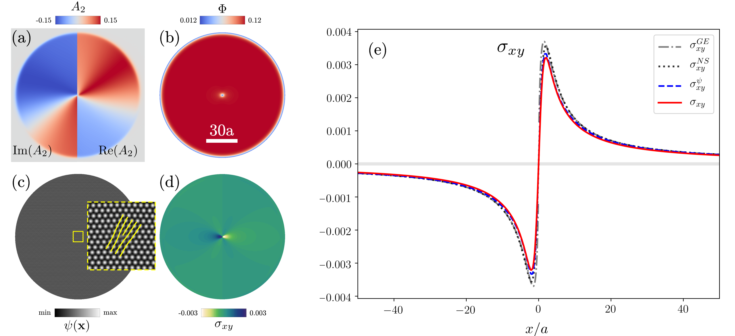
Figure 1: Computation for a configuration with one edge dislocation in a finite crystal, with $\mathbf{b}=(a,0)$. (a) Real (right) and imaginary (left) parts of the amplitude $A_{2}$. (b) $\Phi=2\sum_{j}^{N}|A_{j}|^{2}$. (c) Reconstructed $\psi(\mathbf{x})$ from Eq. (3), with an inset showing a magnification of the small region around the defect. (d) $\sigma_{xy}$. Panels (a)–(d) are obtained with $R=60a$. (e) Comparison between $\sigma_{xy}$, $\sigma_{xy}^{\psi}$, $\sigma_{xy}^{\rm NS}$ and $\sigma_{xy}^{\rm GE}$ along the horizontal line crossing the defect core, for $R=300a$.

The results obtained at $t=100$ are shown in Fig. 1(a)–(d): $A_{2}$ (both real and imaginary parts), $\Phi$ (see Eq. (4)), $\psi(\mathbf{x})$, and $\sigma_{xy}$ for $R=60a$. Figure 1(e) shows the distribution of $\sigma_{xy}^{\psi}$, from Eq. (16), and $\sigma_{xy}$ from Eq. (14) along the horizontal line through the dislocation core. Here we set $R=300a$ to avoid significant influence of the solid-liquid interface, and of the finite size of the crystal on the elastic field of the dislocation. Since the configuration shown is in equilibrium, $\sigma_{xy}^{\psi}$ and $\sigma_{xy}$ should be identical. Indeed, the relaxation of the initial state recovers the equilibrium elastic field without the amplitude correction. A very small shift of the stress field is obtained at large distance, which can be ascribed to the presence of the solid-liquid interface. In terms of dislocation self-energy, computed as $\int\boldsymbol{\sigma}^{d}:\boldsymbol{\varepsilon}^{d}d\mathbf{x}$ with $\boldsymbol{\sigma}^{d}$ and $\boldsymbol{\varepsilon}^{d}$ the stress and strain in the system with a single dislocation, a difference of $\sim 1.5\%$ is found when adding $\boldsymbol{\sigma}^{\delta}$ to $\boldsymbol{\sigma}^{\psi}$. It is worth mentioning that the presence of free surfaces, or in general interfaces in inhomogeneous media, affects some features of the elastic field far from the core (Head, 1953, Marzegalli et al., 2013, Anderson et al., 2017). However, a close comparison to this case is beyond the scope of the present investigation.

The stress field given by the APFC model is non-singular at the dislocation core. Our results for the regularized stress field (Fig. 1(e)) agree with the non-singular theory illustrated in Cai et al. (2006), where the components of the stress field are argued to be given by,

$$\begin{split}\sigma_{xx}^{\rm NS}&=-\frac{\mu b_{x}}{2\pi(1-\nu)}\frac{y(3c^{2}+3x^{2}+y^{2})}{(c^{2}+x^{2}+y^{2})^{2}}\\ \sigma_{yy}^{\rm NS}&=-\frac{\mu b_{x}}{2\pi(1-\nu)}\frac{y(c^{2}-x^{2}+y^{2})}{(c^{2}+x^{2}+y^{2})^{2}}\\ \sigma_{xy}^{\rm NS}&=\frac{\mu b_{x}}{2\pi(1-\nu)}\frac{x(3c^{2}+x^{2}-y^{2})}{(c^{2}+x^{2}+y^{2})^{2}}\end{split}$$ (28)

with $\mu$ the shear modulus and $c$ a regularization parameter related to the dimension of the dislocation core. Good numerical agreement with our results is found by setting $c=2b_{x}$. Therefore, the APFC model naturally includes a regularization of the elastic fields at the dislocation core, which deviates from the singular behavior expected from continuum mechanics (Anderson et al., 2017), but without requiring any additional parameters. Eq. (17) shows how this is accomplished: the right-hand side of this equation corresponds to $[\nabla\times\mathbf{B}(\mathbf{r})]_{z}$ (with $z$ labelling the axis perpendicular to the considered 2D system); that is, for the dislocation considered here $\nabla\times(B_{x}(\mathbf{r}),0)=-\partial B_{x}(\mathbf{r})/\partial y\leavevmode\nobreak\ \hat{z}$. This quantity, for the system of Fig. 1, is shown in Fig. 2(a). $-\partial B_{x}(\mathbf{r})/\partial y$ is smooth over a finite size region near the core, indicating the effective spreading of the Burgers vector (instead of the isolated singularity $\mathbf{B}(\mathbf{r})=\mathbf{b}\delta(\mathbf{r}-\mathbf{r}_{0})$, as expected by continuum mechanics). The spreading of the Burgers vector over a small region around the core is the basic assumption of Cai et al. (2006). The procedure allows regularised continuous fields at the dislocation core, while still matching the prediction of standard continuum mechanics away from the core (see Eq. (28)).

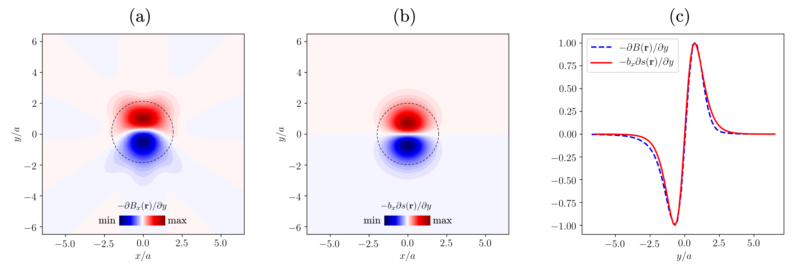
Figure 2: Analysis of the spreading of $\mathbf{b}$. $\nabla\times\mathbf{B}(\mathbf{r})$ is used to illustrate the spreading of the Burgers vector density given by the phase field stress fields, including results of (a) from APFC simulation of a single dislocation, namely the right-hand side of Eq. (17), and (b) from Eq. (29) with $c=2b_{x}$. A circle with radius $c$ is superposed at the origin of plots in panels (a) and (b). (c) Comparison along the vertical line crossing the dislocation core in panels (a) and (b). All the quantities are normalized with respect of the (symmetric) maxima and minima.

More specifically, the non singular theory of (Cai et al., 2006) introduces a spreading function $s(\mathbf{r})$ given by,

$$s(\mathbf{r})=\frac{15}{8\pi c^{3}(r^{2}/c^{2}+1)^{7/2}}.$$ (29)

The convolution of this function with non-singular stress-field components leads to Eqs. (28). Therefore, we can assume a spreading of the Burgers vector density such as $\mathbf{B}^{\rm NS}(\mathbf{r})=(B_{x}^{\rm NS}(\mathbf{r}),0)$ with $B_{x}^{\rm NS}(\mathbf{r})=b_{x}s(\mathbf{r})$ for an edge dislocation having $\mathbf{b}=(b_{x},0)$. Therefore, $\nabla\times B_{x}^{\rm NS}(\mathbf{\mathbf{r}})=-b_{x}\hat{z}\partial s(\mathbf{r})/\partial y$. It is worth mentioning that in Cai et al. (2006), the starting point is to assume a regularization of the Burgers vector density by a function $\tilde{s}(\mathbf{r})$, whose convolution with itself gives Eq. (29). The latter enters the deformation fields and allows the removal of the singularity at the core given that $\int r(\mathbf{x}-\mathbf{x^{\prime}})s(\mathbf{x^{\prime}})d^{3}\mathbf{x^{\prime}}=r_{c}$ with $r_{c}=\sqrt{x^{2}+y^{2}+z^{2}+c^{2}}$. The distribution of $\nabla\times\mathbf{B}_{x}^{\rm NS}(\mathbf{\mathbf{r}})$ is shown in Fig. 2(b) for $c=2b_{x}$. A circle with radius $2b_{x}$ is superposed on both the maps in Figs. 2(a) and (b). In addition, a comparison of the two distributions along the vertical line crossing the defect is shown in Fig. 2(c). The agreement between them indicates that the assumption of isotropic spreading given in Cai et al. (2006) does capture the main features of the regularization at the core given by the APFC model. However, it should be noted that the APFC description naturally incorporates the lattice symmetry and as such will always include any anisotropies in this (or any other) quantity.

Another regularization scheme similar to that discussed above has been introduced by assuming a smooth Burgers vector distribution (Lothe, 1992), or by elasticity theories including first strain-gradient energy terms (Mindlin, 1964, Mindlin and Eshel, 1968). In the so-called Helmoltz type gradient elasticity, for an edge dislocation with Burgers vector oriented along the $x$-axis (i.e., $\mathbf{b}=(b_{x},0)$), the elastic field in an isotropic medium is given by (Lazar and Maugin, 2005, Lazar, 2017)

$$\begin{split}\sigma_{xx}^{\rm GE}&=-\frac{\mu b_{x}}{2\pi(1-\nu)}\frac{y}{r^{4}}\left[(y^{2}+3x^{2})+\frac{4\ell^{2}}{r^{2}}(y^{2}-3x^{2})-2y^{2}\frac{r}{\ell}K_{1}(r/\ell)-2(y^{2}-3x^{2})K_{2}(r/\ell)\right],\\ \sigma_{yy}^{\rm GE}&=-\frac{\mu b_{x}}{2\pi(1-\nu)}\frac{y}{r^{4}}\left[(y^{2}-x^{2})-\frac{4\ell^{2}}{r^{2}}(y^{2}-3x^{2})-2x^{2}\frac{r}{\ell}K_{1}(r/\ell)+2(y^{2}-3x^{2})K_{2}(r/\ell)\right],\\ \sigma_{xy}^{\rm GE}&=\frac{\mu b_{x}}{2\pi(1-\nu)}\frac{x}{r^{4}}\left[(x^{2}-y^{2})-\frac{4\ell^{2}}{r^{2}}(x^{2}-3y^{2})-2y^{2}\frac{r}{\ell}K_{1}(r/\ell)+2(x^{2}-3y^{2})K_{2}(r/\ell)\right],\\ \end{split}$$ (30)

with $K_{n}(r/\ell)$ the modified Bessel function of the second type, and $\ell$ a characteristic internal length parameter of the material. This parameter is usually proportional to the lattice spacing, as has been obtained empirically by comparison with atomistic calculation (see, e.g., (Po et al., 2014)). The elastic field obtained in this approach is also shown in Fig. 1 for $\ell=b_{x}$. With this choice of $\ell$, $\sigma_{\rm xy}^{\rm GE}\approx\sigma_{xy}^{\rm NS}$ within the core region. In turn, both agree with $\sigma_{xy}$ obtained from the APFC model. Within first-gradient elasticity, the spreading of the Burgers vector is given by a function that is singular at the core, $K_{0}(r/\ell)\approx-\left\{\log[r/(2\ell)]+\gamma\right\}\left\{1+r^{2}/(4\ell^{2})\right\}-r^{2}/(4\ell^{2})+\mathcal{O}(r^{4})$ with $\gamma=0.57721...$ the Euler-Mascheroni constant (Lazar, 2017). Therefore an analysis analogous to that of Fig. 2 is not possible. Closer comparisons with this theory will be the subject of future research.

These comparisons shed light on the regularization of stress fields in the (A)PFC framework. Other than the agreement described above, we note that small deviations and asymmetries are observed, in particular concerning the highest stress values obtained in the system (see the curves in Fig. 1(e)). This is, however, expected as nonlinearities are contained in PFC amplitudes (Hüter et al., 2016) which generally capture features on atomic length scales. They would become relevant for large stresses/strains. It is worth mentioning that regularization of the elastic field at the core of a dislocation is natural from an atomistic point of view, as the distribution is expected to be non-singular with vanishing deformation field at the core (see, e.g., Bonilla et al. (2015)) which intrinsically has a finite size. This was also the main argument that led to the renowned Peirels-Nabarro model (Peierls, 1940, Nabarro, 1947), although in this case the resulting elastic fields are discontinuous at the core, even if they do not diverge (Lazar, 2017). Therefore they deviate from the continuous description given by the APFC model.

5.2 Dislocation dipole

In this section a dislocation dipole is considered. The amplitudes are initialized by considering the displacement field of two edge dislocations with Burgers vector $b_{x}=\pm a$ aligned along the $x$ direction. Eqs. (26) and (27) are straightforwardly used by considering $\mathbf{u}(x-x_{0},y-y_{0})$, i.e. shifting the $x$ and $y$ axis to account for the initial position of each dislocation $\mathbf{p}=(x_{0}.y_{0})$. We focus here in particular on two defects having positions $\mathbf{p}_{1,2}=(0,\pm L)$ with $L\sim 10a$. Parameters of the (A)PFC free energy are set as those in Sect. 5.1. A square computational domain with size $200a$ is used, embedding a grain as in the previous section with radius $140a$.

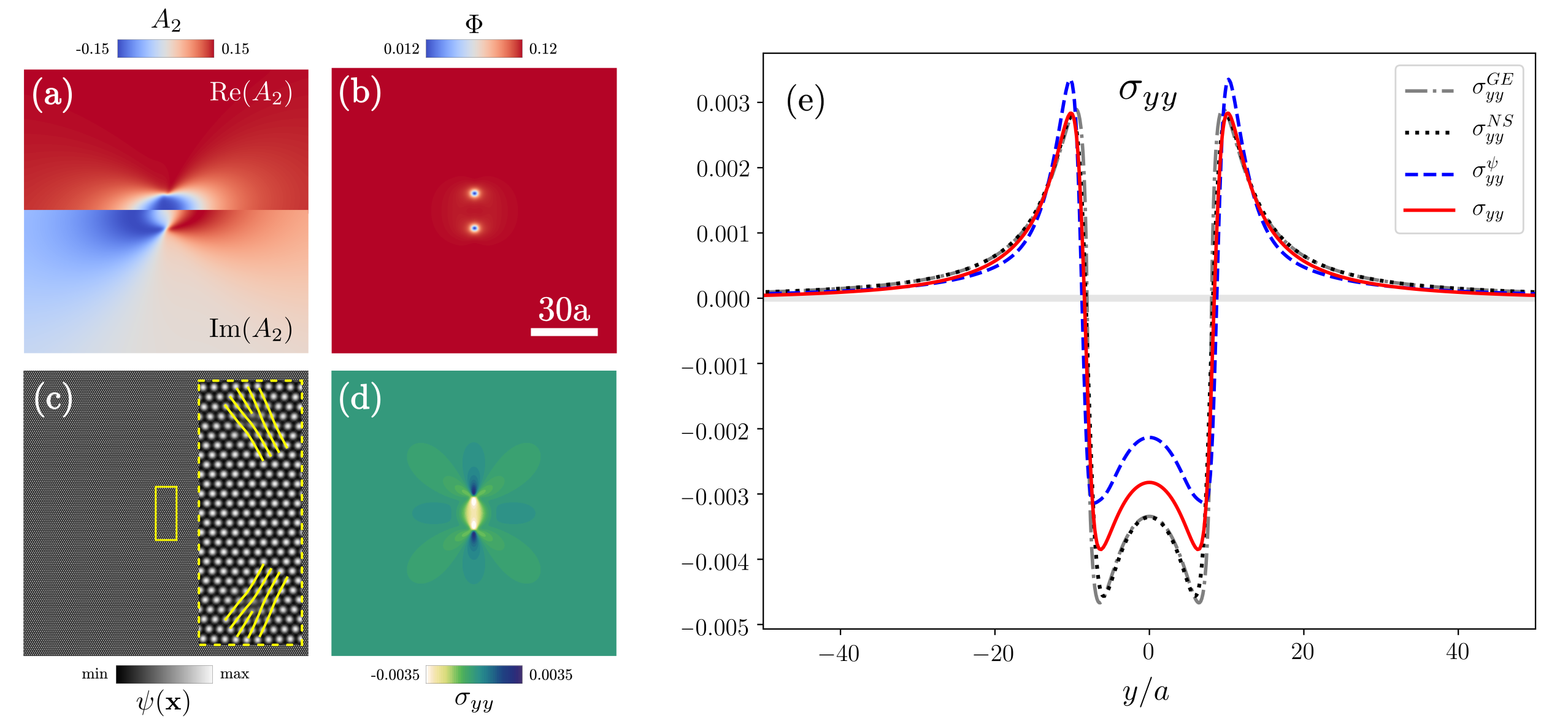
Figure 3: Simulation of an edge-dislocation dipole with $\mathbf{b}_{1,2}=(\pm a,0)$ and positions $\mathbf{p}_{1,2}=(0,\pm 10a)$. (a) Amplitude $A_{2}$ illustrated by its real (top) and imaginary (bottom) parts. (b) $\Phi=2\sum_{j}^{N}|A_{j}|^{2}$. (c) Reconstructed $\psi(\mathbf{x})$ from Eq. (3), with an inset showing a magnification of the small region around the defect. (d) $\sigma_{yy}$. (e) Comparison between $\sigma_{yy}$, $\sigma_{yy}^{\psi}$, $\sigma_{yy}^{\rm NS}$, and $\sigma_{yy}^{\rm GE}$ along a vertical line crossing the defects.

The results obtained at $t=100$ are shown in Fig. 3(a)-(d) which illustrate $A_{2}$, $\Phi$, $\psi(\mathbf{x})$, and $\sigma_{yy}$. The stress fields $\sigma^{\psi}$ and $\sigma$, along with the predictions from non-singular continuum elasticity theories as described in Sect. 5.1 are presented in Fig. 3(e). First, note that the stress $\sigma^{\psi}$ and the total stress $\sigma$ differ from each other, even after a relaxation time from the initial condition which was long enough to obtain a substantial agreement for the case of an isolated dislocation (Sect. 5.1). These APFC results are obtained with parameters corresponding to coexistence of the liquid and solid phases, for which we expect a good description of the elastic relaxation in the standard (A)PFC model, different from deep quenches conditions. The system at $t=100$ is, however, out of equilibrium as the defects will move and finally annihilate. Therefore, as discussed in (Skaugen et al., 2018a), the correction discussed in Sect. 3 is needed to maintain mechanical equilibrium. Note that in Fig. 3(e) the stress fields obtained from continuum elasticity theories, namely Eqs. (28)–(30), have been properly shifted to account for the dislocations forming the dislocation dipole, and are expected to match the PFC elastic field far away from the core (e.g., when $|y|>20a$). Closer to the defects some deviations from continuum elasticity are observed. Such deviations are shown in the regimes of large deformation near dislocation cores (even in the single-dislocation case of Fig. 1). They are more evident in between the individual defects, where the contributions of the two dislocations accumulate. This effect may be ascribed to nonlinearities of elasticity as they are naturally contained in APFC amplitudes and play an important role at high strains (Hüter et al., 2016). In general, they become relevant when the distortion of the lattice parameter $a$ compared to the lattice parameter of the reference crystal, $a_{\rm bulk}$, is $a/a_{\rm bulk}<0.95$ or $a/a_{\rm bulk}<1.05$. Here, strains larger than $5\%$ are observed in the region $|y|<20a$.

5.3 Motion of a dislocation dipole

The configuration of Sect. 5.2 also allows us to investigate the evolution that satisfies the constrain of mechanical equilibrium of elastic distortions as discussed in Sect. 3. We consider here a dislocation dipole with dislocations annihilating by pure glide or climb. We choose as initial conditions two dislocations at $\mathbf{p}_{1,2}=(\pm L,0)$ (configuration G, glide), and $\mathbf{p}_{1,2}=(0,\pm L)$ (configuration C, climb), with $L\sim 15a$. The latter system corresponds to the one analyzed in Sect. 5.2, shown in Fig. 3(a)–(d), while the former consists of the same defects but aligned along the y direction.

Our results are presented in Fig. 4. Panels Fig. 4(a) and Fig. 4(d) show the stress tensor components $\sigma_{xx}$ and $\sigma_{xy}$. Fig. 4(b) and Fig. 4(e) show the position over time of the upper defect for configuration C ($y_{d}$), and of the defect on the right for configuration G ($x_{d}$), respectively. Panels (c) and (f) show the velocity for the two configurations. Model parameters are the same as in Sect. 5.1 and 5.2, corresponding to solid/liquid coexistence. As a first observation, a faster dynamics is obtained when enforcing mechanical equilibrium in PFC, in agreement with (Skaugen et al., 2018b, a). From a macroscopic point of view, the motion of a dislocation can be described in terms of the Peach-Koehler force (Anderson et al., 2017), that is, $f=(\boldsymbol{\sigma}\cdot\mathbf{b})\times\boldsymbol{\xi}$ with $\boldsymbol{\xi}$ the unit vector oriented along the dislocation line, $\mathbf{b}$ the Burgers vector of the dislocation, and $\boldsymbol{\sigma}$ the external elastic field (for a recent review see (Lubarda, 2019)). For the configurations considered here, the force acting on a dislocation is $f_{\rm G}=\sigma_{xy}b$ and $f_{\rm C}=\sigma_{xx}b$, with $\sigma_{ij}$ the stress field generated by the other dislocation. Within the (A)PFC framework, the velocity of the dislocations due to the action of the Peach-Kohler force is given by (Skaugen et al., 2018b)

$$v_{i}^{PK}=\frac{1}{4\pi\phi^{2}}\epsilon_{ij}\sigma_{jk}b_{k}.$$ (31)

This velocity is shown in Figs. 4(b) and (d) for configurations C and G, respectively, using equations given in Sect. 5.1 to compute $\sigma_{ij}$. Notice that it is in good agreement with $v_{x}^{\rm G}=v_{y}^{\rm C}=b^{2}/(2\pi^{2}d)$ (Skaugen et al., 2018b) (they match for $\nu=1/4$). Note that the purely diffusive dynamics of the APFC model significantly underestimates the magnitude of the velocities. By constraining the stress field so that the evolving configuration remains in mechanical equilibrium, the computed velocity agrees well with the prediction based on the Peach-Kohler force.

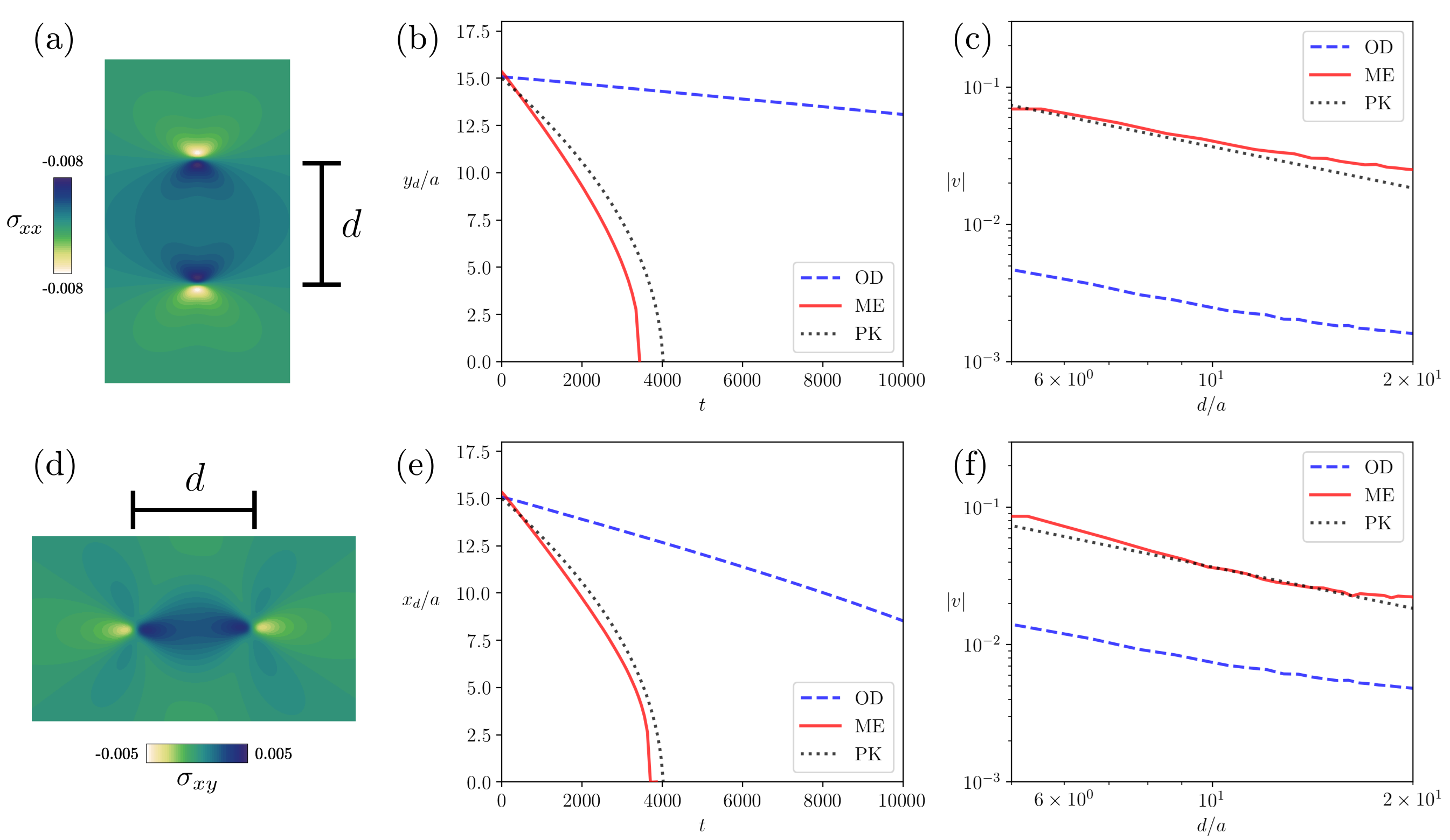
Figure 4: Defect annihilation. For configuration C: (a) $\sigma_{xx}$, (b) position ($y_{d}/a$) over time over time, and (c) velocity. For configuration G: (d) $\sigma_{xy}$, (e) position ($x_{d}/a$) over time, and (f) velocity. In this and other figures, OD, ME and PK refer to overdamped dynamics (the original APFC model), mechanical equilibrium (the present work) and the Peach-Kohler result (Eq. (31)), respectively.

We mention that, from a microscopic point of view, the evolution of configurations C and G are expected to be significantly different. Glide is the movement of dislocations along their slip planes, whereas climb is the motion perpendicular to the slip plane. Both are activated processes over different types of barriers. In the former, a layer of atoms slips over the Peierls-Nabarro barrier, whereas the latter requires the absorption (or emission) of vacancies (Anderson et al., 2017). The first effect can be captured in the standard PFC model (Boyer and Viñals, 2002, Skaugen et al., 2018b) which includes atomic scale microscopic features that are not present in the APFC model (Huang, 2013). Still, at variance with continuum models based solely on mechanics, temperature is included in the APFC approach in a phenomenological fashion as it enters the energy of the ordered and disordered phases. This can be seen, for instance, when changing values of $\Delta B_{0}$. We recall that $\Delta B_{0}=8t^{2}/(135v)$ allows for the coexistence of solid and liquid phases, $\Delta B_{0}\gtrless 8t^{2}/(135v)$ favors the liquid or solid phase, while $\Delta B_{0}\ll 8t^{2}/(135v)$ corresponds to a deep-quench condition. We have verified that increasing $\Delta B_{0}$ (up to the solid-liquid coexistence condition) speeds up defect motion thus capturing, at least qualitatively, the expected change in defect mobility, although no barriers are explicitly included in the APFC model.

5.4 Grain shrinkage

We consider here a 2D system with a rotated grain embedded in a crystalline matrix of triangular symmetry. The grain boundary consists of a series of dislocations that move together. Amplitudes are initialized as (Salvalaglio et al., 2017)

$$A_{j}=\phi_{j}\text{exp}\left(i\delta\mathbf{q}_{j}(\theta)\cdot\mathbf{x}\right),$$ (32)

with

$$\delta\mathbf{q}_{j}(\theta)=\left[q^{x}_{j}(\cos\theta-1)-q^{y}_{j}\sin\theta\right]\hat{\mathbf{x}}+\left[q^{x}_{j}\sin\theta+q^{y}_{j}(\cos\theta-1)\right]\hat{\mathbf{y}}.$$ (33)

$\theta=0$ at a distance $R_{0}$ from the center of the rotated inclusion/grain, which is tilted by an angle $\theta$ with respect to the surrounding matrix. The spatial distributions of $A_{2}$, $\Phi$, $\psi(\mathbf{x})$, and $\sigma_{xx}^{\psi}$, corresponding to $\theta=5^{\circ}$ and $R_{0}=25\pi$, are shown in Fig.5. The parameters of the APFC model are set to be the same as those in the previous sections. The circular grain considered here shrinks over time, which is qualitatively well described by the APFC model (Heinonen et al., 2016, Salvalaglio et al., 2018, 2019). Results of the normalized area $R^{2}(t)/R^{2}_{\rm ini}$ of the shrinking grain with and without the correction described in Sect. 3 are shown in Fig. 6.

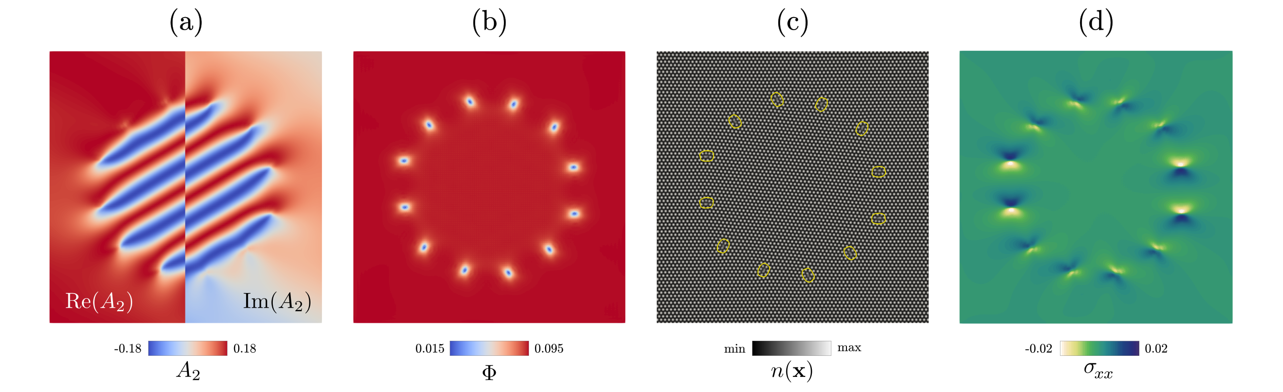
Figure 5: Defects at a circular low-angle grain boundary between a rotated inclusion and an unrotated crystal matrix of triangular symmetry. (a) Amplitude $A_{2}$ illustrated by its real (left) and imaginary (right) parts. (b) $\Phi=2\sum_{j}^{N}|A_{j}|^{2}$. (c) Reconstructed $\psi(\mathbf{x})$ from Eq. (3), with yellow isolines of $\Phi$ highlighting the defects. (d) $\sigma_{xx}$.

For this configuration, the three expressions of the amplitudes corrected by $\mathbf{u}^{\delta}$, namely Eqs. (8), (9) or (10) reported in Sect. 3, are used. In all the cases considered, $R^{2}(t)$ decreases linearly with time. A significantly faster decrease is observed when mechanical equilibrium is imposed, as has also been observed for the evolution of dislocation dipoles in Sect. 5.3 and, for this configuration in particular, in (Heinonen et al., 2016). In agreement with our results, the work reported in Heinonen et al. (2016), in the limit of fast relaxation of elastic excitations, also shows that grain-shrinking dynamics is an order of magnitude faster when accounting for instantaneous mechanical equilibrium. The substantial agreement between three different approaches for correcting the amplitudes (i.e., Eqs. (8), (9) and (10)) supports the assumption of small deformations and slowly varying amplitudes.

The analysis of Sect. 5.1 concerning how lattice distortion follows from the Burgers vector density $\mathbf{B}(\mathbf{r})$, can be readily applied to this configuration to gain insights about the crystal defects in the rotated inclusion and, more in general, in systems with many defects. The spatial distribution $[\nabla\times\mathbf{B}(\mathbf{r})]_{z}$, computed as the right-hand side of Eq. (17) for a rotated inclusion with $\theta=10^{\circ}$ and $R\sim 20a$, is shown in Fig. 7(a). We obtain a localized distribution centered at defects, as in Fig. 2(a). By looking at the arrangement of positive and negative lobes of the distribution, six different orientations are obtained, which correspond to multiples of $30^{\circ}$, consistent with the lattice vectors of the triangular lattice. Indeed, this quantity fully describes the distribution of $\mathbf{b}$ in 2D. Following the arguments of Sect. 5.1, we can identify the orientation of the Burgers vector as being perpendicular to the line connecting the local minimum and maximum of $[\nabla\times\mathbf{B}(\mathbf{r})]_{z}$ at defect cores. This is illustrated in Fig. 7(b). The extension of the local non-zero distributions of $[\nabla\times\mathbf{B}(\mathbf{r})]_{z}$ at defects, as well as its maximum and minimum, are then connected to the Burgers vector. Here they are all equivalent as they should yield $|\mathbf{b}|=a$ for symmetry reasons. Fig. 7(c) gives a schematic illustration of defects with the orientations obtained. Note that the distribution of defects is symmetric, and the sum of all the $\mathbf{b}$’s is zero. It is worth mentioning that for this dynamical system, at variance with Sect. 5.1, the number of defects and the orientation of individual defects are not known a priori. Therefore, this analysis can be used to extract information on the nature of the defects and their evolution towards equilibrium, which is fully contained in the APFC model.

Figure 6: Time evolution of the normalized area of rotated grain, for the overdamped dynamics (OD) and with the correction to amplitudes for mechanical equilibrium (ME) as in Eqs. (8)–(10).

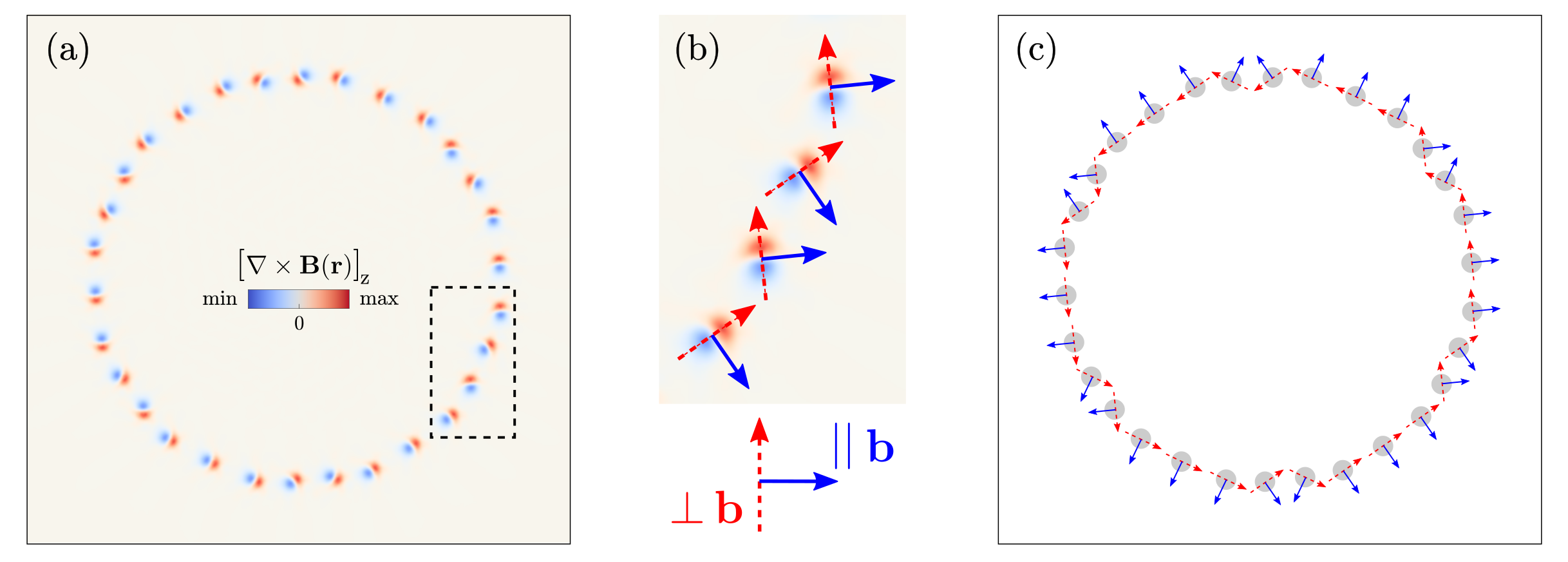
Figure 7: Analysis of the lattice deformation for a rotated inclusion with $\theta=10^{\circ}$ and $R\sim 20a$. (a) $[\nabla\times\mathbf{B}(\mathbf{r})]_{z}$. (b) Detail inside the dashed box of (a), showing the identification of the directions perpendicular (red, dashed arrow) and parallel (blue, solid arrow) to the Burgers vector $\mathbf{b}$. (c) Schematics reporting the scheme of panel (b), where the grey circles (with radius $\sim 2a$) correspond to the positions of individual defects.

6 Conclusions

We have presented a coarse-grained model of lattice distortion and plastic motion as described by the phase-field crystal model in its amplitude expansion formulation. For a system in equilibrium, we have studied the stress field induced by an isolated dislocation, including the regularized stress near the dislocation core. Although the APFC approach cannot provide a detailed description of dislocation cores from an atomistic point of view due to its underlying assumptions (Goldenfeld et al., 2005, 2006, Yeon et al., 2010), we have shown that the resulting deformation fields near the core are smooth, and are generally in agreement with other theories based on continuum elasticity (Lazar and Maugin, 2005, Cai et al., 2006). Concerning plastic flow, the APFC model has been extended to account for fast elastic relaxation by not only determining the incompatible stress from the phase field, but also introducing a compatible distortion to satisfy elastic equilibrium at all times (Skaugen et al., 2018a). The modified model not only agrees well with predictions from continuum elasticity, but it can also include lattice symmetry, naturally account for the formation and motion of topological defects, and computationally, access large system sizes and long time scales (Salvalaglio et al., 2019, Praetorius et al., 2019). Despite the coarse-grained nature of the model, it can provide information about individual defects and defect distributions directly from APFC model variables. In particular, we have shown how to compute the Burgers vector density and its motion from the model amplitudes.

Future work will be devoted to deepen the connections with theories based on continuum mechanics, to extend the results to other lattice symmetries, and to the investigation of three-dimensional systems. The possibility to account for changes in the local average density of the crystal (which is assumed to be constant here) will also be explored. It will allow the extension to the study of binary systems (Elder et al., 2010), and to include a better description of elastic constants (Wang et al., 2018, Ainsworth and Mao, 2019).

References

- Acharya (2001) A. Acharya. A model of crystal plasticity based on the theory of continuously distributed dislocations. J. Mech. Phys. Solids, 49(4):761–784, 2001.
- Adland et al. (2013) A. Adland, A. Karma, R. Spatschek, D. Buta, and M. Asta. Phase-field-crystal study of grain boundary premelting and shearing in bcc iron. Phys. Rev. B, 87:024110, 2013.
- Ainsworth and Mao (2019) M. Ainsworth and Z. Mao. Phase field crystal based prediction of temperature and density dependence of elastic constants through a structural phase transition. Phys. Rev. B, 100:104101, 2019.
- Anderson et al. (2017) P. Anderson, J. Hirth, and J. Lothe. Theory of Dislocations. Cambridge University Press, 2017. ISBN 9780521864367.
- Archer et al. (2019) A. Archer, D. Ratliff, A. Rucklidge, and P. Subramanian. Deriving phase field crystal theory from dynamical density functional theory: consequences of the approximations. Phys. Rev. E, 100:022140, 2019.
- Athreya et al. (2006) B. P. Athreya, N. Goldenfeld, and J. A. Dantzig. Renormalization-group theory for the phase-field crystal equation. Phys. Rev. E, 74(1):011601, 2006.
- Backofen et al. (2014) R. Backofen, K. Barmak, K. Elder, and A. Voigt. Capturing the complex physics behind universal grain size distributions in thin metallic films. Acta Mater., 64:72–77, 2014.
- Berry et al. (2006) J. Berry, M. Grant, and K. R. Elder. Diffusive atomics dynamics of edge dislocations in two dimensions. Phys. Rev. E, 73:031609, 2006.
- Bonilla et al. (2015) L. L. Bonilla, A. Carpio, C. Gong, and J. H. Warner. Measuring strain and rotation fields at the dislocation core in graphene. Phys. Rev. B, 92:155417, 2015.
- Boyer and Viñals (2002) D. Boyer and J. Viñals. Weakly nonlinear theory of grain boundary motion in patterns with crystalline symmetry. Phys. Rev. Lett., 89:055501, 2002.
- Bulatov and Cai (2006) V. Bulatov and W. Cai. Computer Simulations of Dislocations. Oxford University Press, Oxford, 2006.
- Cai et al. (2006) W. Cai, A. Arsenlis, C. Weinberger, and V. Bulatov. A non-singular continuum theory of dislocations. J. Mech. Phys. Solids, 54(3):561–587, 2006.
- Clayton and Knap (2016) J. Clayton and J. Knap. Phase field modeling and simulation of coupled fracture and twinning in single crystals and polycrystals. Comput. Methods Appl. Mech. Eng., 312:447–467, 2016.
- Devincre et al. (1992) B. Devincre, V. Pontikis, Y. Brechet, G. Canova, M. Condat, and L. Kubin. Three-dimensional simulations of plastic flow in crystals. In M. Mareschal and B. L. Holian, editors, Microscopic Simulations of Complex Hydrodynamic Phenomena, pages 413–423. Springer US, Boston, MA, 1992. ISBN 978-1-4899-2314-1.
- Elder and Grant (2004) K. R. Elder and M. Grant. Modeling elastic and plastic deformations in nonequilibrium processing using phase field crystals. Phys. Rev. E, 70(5):051605, 2004.
- Elder et al. (2002) K. R. Elder, M. Katakowski, M. Haataja, and M. Grant. Modeling Elasticity in Crystal Growth. Phys. Rev. Lett., 88:245701, 2002.
- Elder et al. (2007) K. R. Elder, N. Provatas, J. Berry, P. Stefanovic, and M. Grant. Phase-field crystal modeling and classical density functional theory of freezing. Phys. Rev. B, 75:064107, 2007.
- Elder et al. (2010) K. R. Elder, Z.-F. Huang, and N. Provatas. Amplitude expansion of the binary phase-field-crystal model. Phys. Rev. E, 81:011602, 2010.
- Emmerich et al. (2012) H. Emmerich, H. Löwen, R. Wittkowski, T. Gruhn, G. I. Tóth, G. Tegze, and L. Gránásy. Phase-field-crystal models for condensed matter dynamics on atomic length and diffusive time scales: an overview. Adv. Phys., 61:665–743, 2012.
- Goldenfeld et al. (2005) N. Goldenfeld, B. P. Athreya, and J. A. Dantzig. Renormalization group approach to multiscale simulation of polycrystalline materials using the phase field crystal model. Phys. Rev. E, 72:020601, 2005.
- Goldenfeld et al. (2006) N. Goldenfeld, B. P. Athreya, and J. A. Dantzig. Renormalization Group Approach to Multiscale Modelling in Materials Science. J. Stat. Phys., 125:1015–1023, 2006.
- Head (1953) A. K. Head. Edge dislocations in inhomogeneous media. Proc. Phys. Soc. Lond. Sect. B, 66(9):793–801, 1953.
- Heinonen et al. (2014) V. Heinonen, C. V. Achim, K. R. Elder, S. Buyukdagli, and T. Ala-Nissila. Phase-field-crystal models and mechanical equilibrium. Phys. Rev. E, 89(3):032411, 2014.
- Heinonen et al. (2016) V. Heinonen, C. V. Achim, J. M. Kosterlitz, S.-C. Ying, J. Lowengrub, and T. Ala-Nissila. Consistent Hydrodynamics for Phase Field Crystals. Phys. Rev. Lett., 116:024303, 2016.
- Hirvonen et al. (2016) P. Hirvonen, M. M. Ervasti, Z. Fan, M. Jalalvand, M. Seymour, S. M. V. Allaei, N. Provatas, A. Harju, K. R. Elder, and T. Ala-Nissila. Multiscale modeling of polycrystalline graphene: a comparison of structure and defect energies of realistic samples from phase field crystal models. Phys. Rev. B, 94(3):035414, 2016.
- Huang (2013) Z.-F. Huang. Scale-coupling and interface-pinning effects in the phase-field-crystal model. Phys. Rev. E, 87:012401, 2013.
- Hüter et al. (2016) C. Hüter, M. Friák, M. Weikamp, J. Neugebauer, N. Goldenfeld, B. Svendsen, and R. Spatschek. Nonlinear elastic effects in phase field crystal and amplitude equations: Comparison to ab initio simulations of bcc metals and graphene. Phys. Rev. B, 93:214105, 2016.
- Köhler et al. (2016) C. Köhler, R. Backofen, and A. Voigt. Stress induced branching of growing crystals on curved substrates. Phys. Rev. Lett., 16:135502, 2016.
- Koslowski et al. (2002) M. Koslowski, A. M. Cuitino, and M. Ortiz. A phase-field theory of dislocation dynamics, strain hardening and hysteresis in ductile single crystals. J. Mech. Phys. Solids, 50(12):2597–2635, 2002.
- Kubin and Canova (1992) L. Kubin and G. Canova. The modelling of dislocation patterns. Scr. Metall. Mater., 27(8):957 – 962, 1992.
- Lazar (2017) M. Lazar. Non-singular dislocation continuum theories: strain gradient elasticity vs. peierls–nabarro model. Philos. Mag., 97(34):3246–3275, 2017.
- Lazar and Maugin (2005) M. Lazar and G. A. Maugin. Nonsinguazaar stress and strain fields of dislocations and disclinations in first strain gradient elasticity. Int. J. Eng. Sci., 43(13):1157 – 1184, 2005.
- Li et al. (2018) J. Li, B. Ni, T. Zhang, and H. Gao. Phase field crystal modeling of grain boundary structures and growth in polycrystalline graphene. J. Mech. Phys. Solids, 120:36–48, 2018.
- Lothe (1992) J. Lothe. Chapter 2 - dislocations in continuous elastic media. In V. Indenbom and J. Lothe, editors, Elastic Strain Fields and Dislocation Mobility, volume 31 of Modern Problems in Condensed Matter Sciences, pages 175 – 235. Elsevier, 1992.
- Lubarda (2019) V. A. Lubarda. Dislocation Burgers vector and the Peach–Koehler force: a review. J. Mater. Res. Technol., 8(1):1550 – 1565, 2019.
- Majaniemi and Grant (2007) S. Majaniemi and M. Grant. Dissipative phenomena and acoustic phonons in isothermal crystals: A density-functional theory study. Phys. Rev. B, 75:054301, 2007.
- Marzegalli et al. (2013) A. Marzegalli, M. Brunetto, M. Salvalaglio, F. Montalenti, G. Nicotra, M. Scuderi, C. Spinella, M. De Seta, and G. Capellini. Onset of plastic relaxation in the growth of ge on si(001) at low temperatures: atomic-scale microscopy and dislocation modeling. Phys. Rev. B, 88:165418, 2013.
- Mianroodi and Svendsen (2015) J. R. Mianroodi and B. Svendsen. Atomistically determined phase-field modeling of dislocation dissociation, stacking fault formation, dislocation slip, and reactions in fcc systems. J. Mech. Phys. Solids, 77:109–122, 2015.
- Mindlin and Eshel (1968) R. Mindlin and N. Eshel. On first strain-gradient theories in linear elasticity. Int. J. Solids Struct., 4(1):109 – 124, 1968.
- Mindlin (1964) R. D. Mindlin. Micro-structure in linear elasticity. Arch. Ration. Mech. Anal., 16(1):51–78, 1964.
- Nabarro (1947) F. R. N. Nabarro. Dislocations in a simple cubic lattice. Proc. Phys. Soc. London, 59(2):256–272, 1947.
- Peierls (1940) R. Peierls. The size of a dislocation. Proc. Phys. Soc. Lond., 52(1):34–37, 1940.
- Po et al. (2014) G. Po, M. Lazar, D. Seif, and N. Ghoniem. Singularity-free dislocation dynamics with strain gradient elasticity. J. Mech. Phys. Solids, 68:161 – 178, 2014.
- Praetorius et al. (2019) S. Praetorius, M. Salvalaglio, and A. Voigt. An efficient numerical framework for the amplitude expansion of the phase-field crystal model. Model. Simul. Mater. Sci. Eng., 27(4):044004, 2019.
- Rodney et al. (2003) D. Rodney, Y. L. Bouar, and A. Finel. Phase field methods and dislocations. Acta Mater., 51(1):17 – 30, 2003.
- Rollett et al. (2015) A. Rollett, G. Rohrer, and R. Suter. Understanding materials microstructure and behavior at the mesoscale. MRS Bull., 40(11):951–960, 2015.
- Salvalaglio et al. (2017) M. Salvalaglio, R. Backofen, A. Voigt, and K. R. Elder. Controlling the energy of defects and interfaces in the amplitude expansion of the phase-field crystal model. Phys. Rev. E, 96(2):023301, 2017.
- Salvalaglio et al. (2018) M. Salvalaglio, R. Backofen, K. R. Elder, and A. Voigt. Defects at grain boundaries: a coarse-grained, three-dimensional description by the amplitude expansion of the phase-field crystal model. Phys. Rev. Mater., 2(5):053804, 2018.
- Salvalaglio et al. (2019) M. Salvalaglio, A. Voigt, and K. R. Elder. Closing the gap between atomic-scale lattice deformations and continuum elasticity. NPJ Comput. Mater., 5(1):48, 2019.
- Sethna et al. (2017) J. P. Sethna, M. K. Bierbaum, K. A. Dahmen, C. P. Goodrich, J. R. Greer, L. X. Hayden, J. P. Kent-Dobias, E. D. Lee, D. B. Liarte, X. Ni, K. N. Quinn, A. Raju, D. Z. Rocklin, A. Shekhawat, and S. Zapperi. Deformation of crystals: connections with statistical physics. Annu. Rev. Mat. Research, 47(1):217–246, 2017.
- Skaugen et al. (2018a) A. Skaugen, L. Angheluta, and J. Viñals. Separation of elastic and plastic timescales in a phase field crystal model. Phys. Rev. Lett, 121:255501, 2018a.
- Skaugen et al. (2018b) A. Skaugen, L. Angheluta, and J. Viñals. Dislocation dynamics and crystal plasticity in the phase-field crystal model. Phys. Rev. B, 97(5):054113, 2018b.
- Spatschek and Karma (2010) R. Spatschek and A. Karma. Amplitude equations for polycrystalline materials with interaction between composition and stress. Phys. Rev. B, 81(21):214201, 2010.
- Stefanovic et al. (2006) P. Stefanovic, M. Haataja, and N. Provatas. Phase-field crystals with elastic interactions. Phys. Rev. Lett., 96:225504, 2006.
- Stefanovic et al. (2009) P. Stefanovic, M. Haataja, and N. Provatas. Phase field crystal study of deformation and plasticity in nanocrystalline materials. Phys. Rev. E, 80:046107, 2009.
- van Teeffelen et al. (2009) S. van Teeffelen, R. Backofen, A. Voigt, and H. Löwen. Derivation of the phase-field-crystal model for colloidal solidification. Phys. Rev. E, 79:051404, 2009.
- Vey and Voigt (2007) S. Vey and A. Voigt. AMDiS: Adaptive MultiDimensional Simulations. Comput. Vis. Sci., 10(1):57–67, 2007.
- Wang and Li (2010) Y. Wang and J. Li. Phase field modeling of defects and deformation. Acta Mater., 58(4):1212–1235, 2010.
- Wang et al. (2001) Y. Wang, Y. Jin, A. Cuitino, and A. Khachaturyan. Nanoscale phase field microelasticity theory of dislocations: model and 3d simulations. Acta Mater., 49:1847, 2001.
- Wang et al. (2018) Z.-L. Wang, Z.-F. Huang, and Z. Liu. Elastic constants of stressed and unstressed materials in the phase-field crystal model. Phys. Rev. B, 97:144112, 2018.
- Witkowski et al. (2015) T. Witkowski, S. Ling, S. Praetorius, and A. Voigt. Software concepts and numerical algorithms for a scalable adaptive parallel finite element method. Adv. Comput. Math., 41:1145, 2015.
- Wu and Voorhees (2009) K.-A. Wu and P. W. Voorhees. Stress-induced morphological instabilities at the nanoscale examined using the phase field crystal approach. Phys. Rev. B, 80(12):125408, 2009.
- Yeon et al. (2010) D.-H. Yeon, Z.-F. Huang, K. Elder, and K. Thornton. Density-amplitude formulation of the phase-field crystal model for two-phase coexistence in two and three dimensions. Philos. Mag., 90(1-4):237–263, 2010.
- Zhang and Acharya (2018) C. Zhang and A. Acharya. On the relevance of generalized disclinations in defect mechanics. J. Mech. Phys. Solids, 119:188–223, 2018.
- Zhang et al. (2018) C. Zhang, A. Acharya, and S. Puri. Finite element approximation of fields of bulk and interfacial line defects. J. Mech. Phys. Solids, 114:258, 2018.
- Zhang et al. (2015) X. Zhang, A. Acharya, N. J. Walkington, and J. Bielak. A single theory for some quasi-static, supersonic, atomic, and tectonic scale applications of dislocations. J. Mech. Phys. Solids, 84:145–195, 2015.
- Zhou et al. (2019a) W. Zhou, J. Wang, B. Lin, Z. Wang, J. Li, and Z.-F. Huang. Yielding and jerky plasticity of tilt grain boundaries in high-temperature graphene. Carbon, 153:242–256, 2019a.
- Zhou et al. (2019b) W. Zhou, J. Wang, Z. Wang, and Z.-F. Huang. Mechanical relaxation and fracture of phase field crystals. Phys. Rev. E, 99:013302, 2019b.