\startlocaldefs\endlocaldefs

and

t1Supported by an Australian Postgraduate Award. t2All authors are supported in part by the Australian Research Council (Discovery Grant DP150101459 and the ARC Centre of Excellence for Mathematical and Statistical Frontiers, CE140100049).

Fast approximate simulation of finite long-range spin systems

Ross McVinishlabel=e2]r.mcvinish@uq.edu.au [    Liam Hodgkinsonlabel=e1]liam.hodgkinson@uqconnect.edu.au [ University of Queensland School of Mathematics and Physics
University of Queensland
St. Lucia, Brisbane
Queensland, 4072
Australia

E-mail:Β  e1
Abstract

Tau leaping is a popular method for performing fast approximate simulation of certain continuous time Markov chain models typically found in chemistry and biochemistry. This method is known to perform well when the transition rates satisfy some form of scaling behaviour. In a similar spirit to tau leaping, we propose a new method for approximate simulation of spin systems which approximates the evolution of spin at each site between sampling epochs as an independent two-state Markov chain. When combined with fast summation methods, our method offers considerable improvement in speed over the standard Doob-Gillespie algorithm. We provide a detailed analysis of the error incurred for both the number of sites incorrectly labelled and for linear functions of the state.

60H35,
60K35, 65C99,
Tau-leaping, simulation, spin system, error analysis, rate of convergence, mean-field models,
keywords:
[class=MSC]
keywords:

1 Introduction

Finite spin systems are continuous-time Markov chains on $\{0,1\}^{S}$, where $S$ is a finite collection of sites, and the value at only one site changes in each transition. Special cases include the contact process, voter model and Ising model. While great advances have been made in the analysis of these systems in relation to qualitative issues such as phase transitions, rates of convergence, and central limit theorems [26, 27, 28], to address more quantitative questions it is often necessary to employ simulation. As a finite-state continuous-time Markov chain, sample paths can be constructed from the jump chain and holding time distribution based on the work of Doob [10, 11]. In the chemistry and biochemistry literature this algorithm is often referred to as the Gillespie algorithm following [15, 16]; in the sequel, shall be referred to as the Doob–Gillespie algorithm.

When the number of sites is large, exact simulation over a desired time interval can be infeasible due to prohibitively small expected times between transitions. This issue is not particular to spin systems and arises more generally in the simulation of continuous time Markov chains modelling large populations. Gillespie [17] proposed the tau-leaping method as a means of generating an approximate sample path that avoids this problem. Tau-leaping essentially treats the transition rates as constant over small time intervals. Anderson et al. [2] provide a detailed analysis of resulting error in the sample paths. In principle, tau-leaping could be applied to spin systems, however they lack the scaling required for tau-leaping to provide a reasonable speed-accuracy trade off.

In this paper we propose a new algorithm for the approximate simulation of long-range finite spin systems. The basic idea here is to briefly decouple sites over small time intervals so that the spin system is treated as a collection of independent two-state Markov chains. We provide a detailed analysis of the error in terms of the number of sites incorrectly labelled and accuracy of certain linear functionals of the state. Our analysis is inspired by [2], though we keep our analysis entirely non-asymptotic.

1.1 The basic model

We formulate the class of finite spin systems as continuous-time Markov processes on the state space $\{0,1\}^{n}$ for some positive integer $n$ representing the total number of sites, where simultaneous transitions at multiple distinct sites occurs with zero probability. Any finite spin system $(\eta(t),t\geq 0)$ can be represented as a Markov jump process in the usual transition notation:

$$\begin{aligned} \eta_{i}:\quad 0\to 1&\quad\mbox{at rate }q_{i}^{+}(\eta)\\ 1\to 0&\quad\mbox{at rate }q_{i}^{-}(\eta)\end{aligned}\qquad\mbox{for }i=1,\dots,n.$$

Here, the functions $q_{i}^{+},q_{i}^{-}:\{0,1\}^{n}\to[0,\infty)$ represent the rate at which sites flip to the positive state (1), and the zero state (0), respectively. The function $q(\eta,i)=\eta_{i}q_{i}^{-}(\eta)+(1-\eta_{i})q_{i}^{+}(\eta)$ is often called the rate function of the process [27]. Let $N_{i}^{+}$ and $N_{i}^{-}$ for each $i=1,\dots,n$ be independent unit-rate Poisson processes. Representing the finite spin system $\eta$ as a random time change of Poisson processes [13, Β§6], we find that for any $t\geq 0$,

$$\eta_{i}(t)=\eta_{i}(0)+N_{i}^{+}\left(\int_{0}^{t}(1-\eta_{i}(s))q_{i}^{+}(\eta(s))\mathrm{d}s\right)\\ -N_{i}^{-}\left(\int_{0}^{t}\eta_{i}(s)q_{i}^{-}(\eta(s))\mathrm{d}s\right),\quad i=1,\dots,n.$$ (1)

The focus in this paper is on a predominant subclass of practical spin systems whose $q_{i}^{+}$ and $q_{i}^{-}$ functions are of the general form

$$f_{i}(v_{i}),\quad\mbox{where}\quad v_{i}=\sum_{j=1}^{n}s_{ij}x_{j},$$ (2)

for some functions $f_{i}:\mathbb{R}\to\mathbb{R}_{+}$ and constants $s_{ij}\in\mathbb{R}$ such that the sums $\sum_{j=1}^{n}s_{ij}$ are uniformly bounded independently of $n$. As a model of mean-field type, $\{v_{i}\}_{i=1}^{n}$ are commonly referred to as potentials. Transition rate functions of this form are common in applications such as Hanski’s metapopulation model [22, 1], spatial SIS epidemic model [7, 21], the voter model [27, Β§5] and the Ising model with Kac potentials [8]. They are often considered for their capacity to interact with a very large number of other sites (indeed, the entire system!). The form of (2) suggests that it will be important to understand the evolution of linear functionals of the state. Under certain conditions, the spin system is well approximated by a deterministic system $\rho(t)=(\rho_{i}(t))_{i=1}^{n}$ in the sense that $\sup_{\phi\in\Phi}\left|\sum_{i=1}^{n}\phi_{i}(\eta_{i}(t)-\rho_{i}(t))\right|$ is small for sufficiently regular $\Phi\subset\mathbb{R}^{n}$ [4]. In particular, this deterministic system is given by the solution to

ρi​(t)=ρi​(0)+∫0t(1βˆ’Οi​(s))​qi+​(ρ​(s))βˆ’Οi​(s)​qiβˆ’β€‹(ρ​(s))​d​s,for all ​tβ‰₯0,formulae-sequencesubscriptπœŒπ‘–π‘‘subscriptπœŒπ‘–0superscriptsubscript0𝑑1subscriptπœŒπ‘–π‘ superscriptsubscriptπ‘žπ‘–πœŒπ‘ subscriptπœŒπ‘–π‘ superscriptsubscriptπ‘žπ‘–πœŒπ‘ d𝑠for all 𝑑0\rho_{i}(t)=\rho_{i}(0)+\int_{0}^{t}(1-\rho_{i}(s))q_{i}^{+}(\rho(s))-\rho_{i}(s)q_{i}^{-}(\rho(s))\mathrm{d}s,\quad\mbox{for all }t\geq 0, (3)

assuming that $q_{i}^{+}$ and $q_{i}^{-}$ can be smoothly extended to $[0,1]^{n}$ (see Appendix A).

1.2 Approximate simulation

As noted earlier, finite spin systems can in principle be simulated exactly using the Doob-Gillespie algorithm, though this may be computationally infeasible. Assuming that for each $\eta\in\{0,1\}^{n}$, $\sum_{i=1}^{n}q(\eta,i)=\mathcal{O}(n)$, the expected number of transitions in a sample path on $[0,T]$ is then $\mathcal{O}(nT)$. If each of the transition rates can be updated after a transition in constant time, as is the case for transition rate functions above by storing and updating the potentials, then the computational cost of simulating this sample path using the Doob-Gillespie algorithm is $\mathcal{O}(n^{2}T)$.

Basic tau leaping is ill-suited to simulating spin systems. Fixing some step size $\delta>0$, let $t_{k}\coloneqq k\delta$ denote the lattice of points over which the simulation is carried out. For notational convenience, we define $\chi$ as the simple function

χ​(s)β‰”βˆ‘k=0∞tkβ€‹πŸ™s∈[tk,tk+1).β‰”πœ’π‘ superscriptsubscriptπ‘˜0subscriptπ‘‘π‘˜subscript1𝑠subscriptπ‘‘π‘˜subscriptπ‘‘π‘˜1\chi(s)\coloneqq\sum_{k=0}^{\infty}t_{k}\mathds{1}_{s\in[t_{k},t_{k+1})}.

that maps each time point $t$ to the last point on the lattice. The process of Euler tau-leaping translates to holding the transition rates constant over each interval $[t_{k},t_{k+1})$. With this in mind, the Euler tau-leaping approximation $\hat{\eta}^{\delta}$ to (1) satisfies

$$\hat{\eta}^{\delta}_{i}(t)=\eta_{i}(0)+N_{i}^{+}\left(\int_{0}^{t}(1-\hat{\eta}_{i}^{\delta}\circ\chi(s))\,q_{i}^{+}(\hat{\eta}^{\delta}\circ\chi(s))\mathrm{d}s\right)\\ -N_{i}^{-}\left(\int_{0}^{t}\hat{\eta}_{i}^{\delta}\circ\chi(s)\,q_{i}^{-}(\hat{\eta}^{\delta}\circ\chi(s))\mathrm{d}s\right),\qquad i=1,\dots,n.$$ (4)

At the lattice points, $\hat{\eta}^{\delta}$ can be evaluated recursively via

$$\hat{\eta}^{\delta}_{i}(t_{k+1})=\hat{\eta}^{\delta}_{i}(t_{k})+\Lambda_{i,k}^{+}-\Lambda_{i,k}^{-},$$

where $\Lambda_{i,k}^{+}$ and $\Lambda_{i,k}^{-}$ are independent Poisson random variables with means $\delta\hat{\eta}^{\delta}_{i}q^{+}_{i}(\hat{\eta}^{\delta}(t_{k}))$ and $\delta(1-\hat{\eta}^{\delta}_{i})q^{-}_{i}(\hat{\eta}^{\delta}(t_{k}))$, respectively. For the path of $\hat{\eta}^{\delta}$ to remain in $\{0,1\}^{n}$ it is necessary that the Poisson random variables $\Lambda_{i,k}^{+}$ and $\Lambda_{i,k}^{-}$ are either 0 or 1 for all $i$ and $k$. For this to occur with high probability it is necessary that the step size is $\mathcal{O}(n^{-1})$. The need to take such a small step size removes any benefit to performing tau-leaping.

Motivated by the propagation of chaos results that often hold for this type of system [25, 32, 3], our strategy is to decouple the sites over each time interval $[t_{k},t_{k+1})$ so that the process becomes a system of $n$ independent two-state Markov chains whose transition probabilities are known explicitly. This process never leaves the set $\{0,1\}^{n}$ so avoids the issue described above. However, the quality of the approximation will depend on how well $q_{i}^{+}(\eta(t))$ and $q_{i}^{-}(\eta(t))$ can be approximated over $[t_{k},t_{k+1}]$ by suitably chosen constants. The simplest way of incorporating this idea is via a forward Euler scheme, approximating $q_{i}^{+}(\eta(t))$ and $q_{i}^{-}(\eta(t))$ by their value at the most recent point on the lattice. With this in mind, the Euler approximation $\eta^{\delta}$ to (1) satisfies

$$\eta^{\delta}_{i}(t)=\eta_{i}(0)+N_{i}^{+}\left(\int_{0}^{t}(1-\eta_{i}^{\delta}(s))q_{i}^{+}(\eta_{i}^{\delta}\circ\chi(s))\mathrm{d}s\right)\\ -N_{i}^{-}\left(\int_{0}^{t}\eta_{i}^{\delta}(s)q_{i}^{-}(\eta_{i}^{\delta}\circ\chi(s))\mathrm{d}s\right),\qquad i=1,\dots,n,$$ (5)

The resulting two-state Markov chains on $[t_{k},t_{k+1}]$ can be simulated using the Doob-Gillespie algorithm . Even more convenient is the fact that the transition probabilities of two-state Markov jump processes are known explicitly, and so it is possible to simulate the process at each time point $t_{k}$ as a discrete-time Markov chain. Indeed, by letting $Q_{i}(x)=q_{i}^{+}(x)+q_{i}^{-}(x)$ for each $i=1,\dots,n$, assuming Qi​(x)β‰ 0subscript𝑄𝑖π‘₯0Q_{i}(x)\neq 0, $\mathbb{P}(\eta_{i}^{\delta}(t_{k+1})=1|\eta^{\delta}(t_{k}))=P_{i}^{\delta}(\eta^{\delta}(t_{k}))$, where

$$P_{i}^{\delta}(\eta^{\delta}(t_{k}))\coloneqq\begin{cases}\frac{q_{i}^{+}(\eta^{\delta}(t_{k}))}{Q_{i}(\eta^{\delta}(t_{k}))}(1-e^{-\delta Q_{i}(\eta^{\delta}(t_{k}))})&\mbox{ if }\eta_{i}^{\delta}(t_{k})=0\\ 1-\frac{q_{i}^{-}(\eta^{\delta}(t_{k}))}{Q_{i}(\eta^{\delta}(t_{k}))}(1-e^{-\delta Q_{i}(\eta^{\delta}(t_{k}))})&\mbox{ if }\eta_{i}^{\delta}(t_{k})=1.\end{cases}$$ (6)

Pseudocode for simulating the Euler approximation on the lattice $\{k\delta\}_{k=0}^{N}$ is provided in Algorithm 1.

Input :Β Number of sites $n$, transition rates $q_{i}^{+}$, $q_{i}^{-}$ for $i=1,\dots,n$, initial value $\eta^{\delta}(0)\in\{0,1\}^{n}$, time step $\delta>0$, and number of time steps $N$
Output :Β System state at each time point $\{\eta^{\delta}(\delta),\eta^{\delta}(2\delta),\dots,\eta^{\delta}(N\delta)\}$
Β 
forΒ k=0,…,Nβˆ’1π‘˜0…𝑁1k=0,\ldots,N-1Β do
Β Β Β Β Β Β  forΒ i=1,…,n𝑖1…𝑛i=1,\dots,nΒ do
Β Β Β Β Β Β Β Β Β Β Β Β  Sample $\eta_{i}^{\delta}((k+1)\delta)$ as a Bernoulli random variable with success probability $P_{i}^{\delta}(\eta^{\delta}(k\delta))$.
Β Β Β Β Β Β  end for
Β Β Β Β Β Β 
end for
AlgorithmΒ 1 Simulating the Euler approximation (5) for spin systems

To improve upon the Euler method, a midpoint approximation to qi+​(η​(s))superscriptsubscriptπ‘žπ‘–πœ‚π‘ q_{i}^{+}(\eta(s)) and qiβˆ’β€‹(η​(s))superscriptsubscriptπ‘žπ‘–πœ‚π‘ q_{i}^{-}(\eta(s)) will also be considered. Analogous to the deterministic approximation (3), this requires extending $q_{i}^{+}$ and $q_{i}^{-}$ smoothly to $[0,1]^{n}$. This can be done in an arbitrary manner, but the choice of extension will play a role in the quality of the approximation, and consequently, in the error analysis to follow. Letting $p_{i}^{\delta}(z)\coloneqq z_{i}+\frac{1}{2}\delta q_{i}(z)$ for $z\in[0,1]^{n}$ and each $i=1,\dots,n$, and assuming that $\delta$ is sufficiently small so that $p_{i}^{\delta}$ maps $[0,1]^{n}$ into itself, the midpoint approximation $\mathring{\eta}^{\delta}$ satisfies

$$\mathring{\eta}^{\delta}_{i}(t)=\eta_{i}(0)+N_{i}^{+}\left(\int_{0}^{t}(1-\mathring{\eta}_{i}^{\delta}(s))q_{i}^{+}(p^{\delta}\circ\mathring{\eta}^{\delta}\circ\chi(s))\mathrm{d}s\right)\\ -N_{i}^{-}\left(\int_{0}^{t}\mathring{\eta}_{i}^{\delta}(s)q_{i}^{-}(p^{\delta}\circ\mathring{\eta}^{\delta}\circ\chi(s))\mathrm{d}s\right),\qquad i=1,\dots,n.$$ (7)

This time, the transition probabilities are given by

$$\mathbb{P}(\mathring{\eta}_{i}^{\delta}(t_{k+1})=1|\mathring{\eta}_{i}^{\delta}(t_{k}))=P_{i}^{\delta}(p^{\delta}\circ\mathring{\eta}^{\delta}(t_{k})).$$ (8)

Pseudocode for simulating the midpoint approximation on the lattice $\{k\delta\}_{k=0}^{N}$ is provided in Algorithm 2.

Input :Β Number of sites $n$, transition rates $q_{i}^{+}$, $q_{i}^{-}$ for $i=1,\dots,n$, initial value $\mathring{\eta}^{\delta}(0)\in\{0,1\}^{n}$, time step $\delta>0$, and number of time steps $N$
Output :Β System state at each time point $\{\mathring{\eta}^{\delta}(\delta),\mathring{\eta}^{\delta}(2\delta),\dots,\mathring{\eta}^{\delta}(N\delta)\}$
Β 
forΒ k=0,…,Nβˆ’1π‘˜0…𝑁1k=0,\ldots,N-1Β do
Β Β Β Β Β Β  forΒ i=1,…,n𝑖1…𝑛i=1,\dots,nΒ do
Β Β Β Β Β Β Β Β Β Β Β Β  Compute $\tilde{\eta}_{i}^{\delta}(k\delta)=p_{i}^{\delta}(\mathring{\eta}^{\delta}(k\delta))$.
Β Β Β Β Β Β  end for
Β Β Β Β Β Β forΒ i=1,…,n𝑖1…𝑛i=1,\dots,nΒ do
Β Β Β Β Β Β Β Β Β Β Β Β  Sample $\mathring{\eta}^{\delta}((k+1)\delta)$ as a Bernoulli random variable with success probability $P_{i}^{\delta}(\tilde{\eta}^{\delta}(k\delta))$.
Β Β Β Β Β Β  end for
Β Β Β Β Β Β 
end for
AlgorithmΒ 2 Simulating the midpoint approximation (7) for spin systems

Practically speaking, a single step of Algorithm 2 is not much more challenging to execute than Algorithm 1, only doubling the computation involved. However, as we shall see, the midpoint approximation can be substantially more accurate than the Euler approximation allowing a much larger step size to be taken.

1.3 Fast summation methods

Algorithms 1 and 2 will only be useful if they can be implemented with significantly less computational cost than the Doob-Gillepie algorithm applied to the original process (1). When the functions $q_{i}^{+}$ and $q_{i}^{-}$ have the form (2), naive evaluation of the $2n$ transition rates requires $\mathcal{O}(n^{2})$ operations. In Algorithms 1 and 2 they must be recomputed at every time-step, implying an $\mathcal{O}(n^{2}T/\delta)$ computational burden. On the other hand the computation burden of the Doob-Gillespie algorithm is $\mathcal{O}(n^{2}T)$. Therefore, naively implemented, these algorithms are more costly to implement than the Doob-Gillespie algorithm. For Algorithms 1 and 2 to offer computational savings we need methods which can evaluate $n$ sums of the form (2) in sub-quadratic time.

In the special case where the sites are indexed on a $d$-dimensional regular lattice and si​j=k​(iβˆ’j)subscriptπ‘ π‘–π‘—π‘˜π‘–π‘—s_{ij}=k(i-j) for some kernel function $k$, the sums in (2) become convolutions which may be rapidly computed exactly in $\mathcal{O}(n\log n)$ time using the fast Fourier transform. This approach is simple and well-known, yet remains effective and highly recommended whenever applicable, thanks to the accessibility of highly efficient implementations of the fast Fourier transform [14]. In fact, our numerical experiments will focus predominantly on this particular method.

The state-of-the-art methods in this arena are the class of tree methods and their siblings. When the number of spatial dimensions $d$ is not too large, these comprise perhaps the fastest summation methods to date [18]. The simpler, single-tree case involves the construction of a tree which groups the $n$ sites together in $\mathcal{O}(\log n)$ levels, in $\mathcal{O}(n\log n)$ time. Usually this is performed spatially with respect to some metric (usually Euclidean). By utilising some form of approximation (either spatial averages or multipole expansions), information necessary to estimate potentials can be contained in each group at each level of the tree. For each source site $z_{i}$, the corresponding potential $v_{i}$ can be obtained by passing through each level of the tree. The number of steps required to estimate the potential of a single node becomes $\mathcal{O}(\log n)$, for a total $\mathcal{O}(n\log n)$ computation time. Algorithms of this form include the celebrated Barnes-Hut algorithm [5] commonly used for simulations of the $n$-body problem.

A more sophisticated, and often much more efficient, approach, is to group source sites according to a tree as well. Such methods are referred to as dual–tree methods, and have linear total computation complexity, for a fixed tolerance $\epsilon$ [18]. The most noteworthy dual–tree method is the fast multipole method of Greengard and Rokhlin [19] (including its application to the Gaussian kernel, called the fast Gauss transform [20, 34]). Provided the bandwidth of the kernel is not too small, computation of the potentials can be achieved in $\mathcal{O}(n)$ time. On the other hand, if the bandwidth is too small, the fast multipole method can prove even less efficient than the naive approach.

1.4 Paper outline

The remainder of the paper is organised as follows: first, in Β§2, we develop strong error bounds for the approximations (5) and (7), controlling the expected number of sites with incorrect spin in terms of the step size and norms on the derivatives of $q$. In Β§3, we study the renormalised differences of linear combinations of the state vectors for the Euler method. Unlike the approach seen in [2], ours will be purely non-asymptotic, deriving an explicit error bound on the rate of convergence as well. Together with the strong error bounds, this analysis shows that the mid-point method is substantially more accurate than the Euler method when the system is not in equilibrium. Finally, in Β§4, we empirically demonstrate the accuracy of the approximation and the reduced computational cost of the proposed simulation method. All proofs have been relegated to Appendix B.

2 Strong error analysis

Our analysis begins with the development of strong error bounds for the Euler and midpoint methods. These arguments adhere fairly closely to those of [2], but must take greater care to keep track of terms depending on $n$, especially those involving derivatives of $q^{+}$ and $q^{-}$. For this purpose, it is necessary to introduce some notation. For a function $f:[0,1]^{n}\rightarrow\mathbb{R}^{m}$, let $\|f\|_{\infty}=\max_{i}\sup_{x}|f_{i}(x)|$. Define

$\displaystyle\|Df\|_{1}$ $\displaystyle\coloneqq\max_{j}\sum_{i}\|\partial_{j}f_{i}\|_{\infty},$ $\displaystyle\|D^{\ast}f\|_{1}$ ≔maxjβ€‹βˆ‘iβ‰ jβ€–βˆ‚jfiβ€–βˆž,≔absentsubscript𝑗subscript𝑖𝑗subscriptnormsubscript𝑗subscript𝑓𝑖\displaystyle\coloneqq\max_{j}\sum_{i\neq j}\|\partial_{j}f_{i}\|_{\infty},
$\displaystyle\|Df\|_{\infty}$ $\displaystyle\coloneqq\max_{i}\sum_{j}\|\partial_{j}f_{i}\|_{\infty},$ $\displaystyle\|D^{\ast}f\|_{\infty}$ ≔maxiβ€‹βˆ‘jβ‰ iβ€–βˆ‚jfiβ€–βˆž.≔absentsubscript𝑖subscript𝑗𝑖subscriptnormsubscript𝑗subscript𝑓𝑖\displaystyle\coloneqq\max_{i}\sum_{j\neq i}\|\partial_{j}f_{i}\|_{\infty}.

Since $q_{i}(x)=q_{i}^{+}(x)$ if $x_{i}=0$ and $q_{i}(x)=q_{i}^{-}(x)$ if $x_{i}=1$, it follows that $\|q^{+}\|_{\infty}\leq\|q\|_{\infty}$ and $\|q^{-}\|_{\infty}\leq\|q\|_{\infty}$. Furthermore, by construction, $\partial_{i}q^{+}_{i}(x)=\partial_{i}q^{-}_{i}(x)=0$ and, for jβ‰ i𝑗𝑖j\neq i, $\partial_{j}q_{i}(x)=(1-x_{i})\partial_{j}q^{+}_{i}(x)-x_{i}\partial_{j}q^{-}_{i}(x)$, Therefore, if $p=1$ or $p=\infty$, $\|Dq^{+}\|_{p}\leq\|D^{\ast}q\|_{p}$ and $\|Dq^{-}\|_{p}\leq\|D^{\ast}q\|_{p}$.

With this in tow, the strong error analysis for the Euler method is stated in Theorem 2.1. Note that the only assumption required here is that $q\in\mathcal{C}^{1}([0,1]^{n},\mathbb{R}_{+}^{n})$.

Theorem 2.1.

For some step-size $\delta>0$, let $\eta(t)$ and $\eta^{\delta}(t)$ satisfy (1) and the Euler approximation (5) respectively. Then for any time $T>0$,

$$\sup_{t\in[0,T]}\sum_{i=1}^{n}\mathbb{E}|\eta_{i}(t)-\eta_{i}^{\delta}(t)|\leq 4n\delta T\|q\|_{\infty}\|D^{\ast}q\|_{1}e^{2T(\|q\|_{\infty}+\|D^{\ast}q\|_{1})}.$$

To elucidate the order of approximation of the strong error bound in Theorem 2.1, we return to the aforementioned β€˜mean-field’ case. Here, both $\|q\|_{\infty}$ and $\|D^{\ast}q\|_{1}$ are $\mathcal{O}(1)$, and so the expected number of discrepancies between $\eta(t)$ and the Euler approximation $\eta^{\delta}(t)$ is $\mathcal{O}(n\delta)$. Recalling that the corresponding error for the deterministic approximation is $\mathcal{O}(n^{1/2})$, the Euler approximation can be guaranteed to be competitive only if $\delta=\mathcal{O}(n^{-1/2})$.

We now proceed on to obtain a strong error bound for the midpoint method. The situation here is more complex, now involving second-order derivatives of $q$, so requiring $q\in\mathcal{C}^{2}([0,1]^{n},\mathbb{R}_{+}^{n})$. Once again, we define two variables that control this higher-order regularity:

Ξ³n=βˆ‘i,j=1iβ‰ jnβ€–βˆ‚j2qiβ€–βˆž,andΞ“n=maxi=1,…,nβ€‹βˆ‘j,k=1j,kβ‰ inβ€–βˆ‚jβˆ‚kqiβ€–βˆž.formulae-sequencesubscript𝛾𝑛superscriptsubscript𝑖𝑗1𝑖𝑗𝑛subscriptnormsubscriptsuperscript2𝑗subscriptπ‘žπ‘–andsubscriptΓ𝑛subscript𝑖1…𝑛superscriptsubscriptπ‘—π‘˜1π‘—π‘˜π‘–π‘›subscriptnormsubscript𝑗subscriptπ‘˜subscriptπ‘žπ‘–\gamma_{n}=\sum_{\begin{subarray}{c}i,j=1\\ i\neq j\end{subarray}}^{n}\|\partial^{2}_{j}q_{i}\|_{\infty},\qquad\mbox{and}\qquad\Gamma_{n}=\max_{i=1,\dots,n}\sum_{\begin{subarray}{c}j,k=1\\ j,k\neq i\end{subarray}}^{n}\|\partial_{j}\partial_{k}q_{i}\|_{\infty}.

For a function $f:[0,1]^{n}\to\mathbb{R}^{m}$, we will also require

β€–D​fβ€–2,1=βˆ‘i=1n(βˆ‘j=1nβ€–βˆ‚jfiβ€–βˆž2)1/2,β€–Dβˆ—β€‹fβ€–2,1=βˆ‘i=1m(βˆ‘j=1,jβ‰ inβ€–βˆ‚jfiβ€–βˆž2)1/2.formulae-sequencesubscriptnorm𝐷𝑓21superscriptsubscript𝑖1𝑛superscriptsuperscriptsubscript𝑗1𝑛superscriptsubscriptnormsubscript𝑗subscript𝑓𝑖212subscriptnormsuperscriptπ·βˆ—π‘“21superscriptsubscript𝑖1π‘šsuperscriptsuperscriptsubscriptformulae-sequence𝑗1𝑗𝑖𝑛superscriptsubscriptnormsubscript𝑗subscript𝑓𝑖212\|Df\|_{2,1}=\sum_{i=1}^{n}\left(\sum_{j=1}^{n}\|\partial_{j}f_{i}\|_{\infty}^{2}\right)^{1/2},\ \|D^{\ast}f\|_{2,1}=\sum_{i=1}^{m}\left(\sum_{j=1,j\neq i}^{n}\|\partial_{j}f_{i}\|_{\infty}^{2}\right)^{1/2}.

The strong error bound for the midpoint method is presented in Theorem 2.2.

Theorem 2.2.

Let $\eta(t)$ and $\mathring{\eta}^{\delta}(t)$ satisfy (1) and the midpoint approximation (7) respectively. Then for any step-size $\delta>0$ and any time $T>0$,

$$\sup_{t\in[0,T]}\sum_{i=1}^{n}\mathbb{E}|\eta_{i}(t)-\mathring{\eta}^{\delta}_{i}(t)|\leq 10\alpha(n,\delta)(T+1)e^{2T(\|q\|_{\infty}+\|D^{\ast}q\|_{1})}.$$

where

$$\alpha(n,\delta)=n\delta^{2}\|q\|_{\infty}(1+\|q\|_{\infty})(1+\|D^{\ast}q\|_{1})\left(\Gamma_{n}+\|D^{\ast}q\|_{1}\right)\\ +\delta\|q\|_{\infty}\gamma_{n}+\delta^{1/2}\|q\|_{\infty}^{1/2}\|D^{\ast}q\|_{2,1}.$$

Returning to the mean-field case, both $\gamma_{n}$ and $\Gamma_{n}$ are $\mathcal{O}(1)$, while $\|D^{\ast}q\|_{2,1}$ is $\mathcal{O}(n^{1/2})$, implying the error bound in Theorem 2.2 is of order $\mathcal{O}(n\delta^{2}+(n\delta)^{1/2})$. If $\delta\geq n^{-1/3}$, the $\mathcal{O}(n\delta^{2})$ term dominates as $n\to\infty$, implying that the midpoint method is competitive with the deterministic approximation if $\delta=\mathcal{O}(n^{-1/4})$. Ignoring constants, for large $n$, this suggests that the midpoint method has smaller error than the Euler method for the viable case $\delta\geq n^{-1}$.

3 Exact error asymptotics

Having now established strong error bounds for the two approximation methods, we shall formally demonstrate that the midpoint method should outperform the Euler method in the $n\to\infty$ regime for viable step sizes. To accomplish this, we will prove that the $\mathcal{O}(n\delta)$ error complexity is exact by characterising the limiting behaviour of weighted errors

$$(n\delta)^{-1}\sum_{i=1}^{n}\phi_{i}(\eta_{i}(t)-\eta^{\delta}_{i}(t)),\quad\phi_{i}\in\mathbb{R},$$

between the finite spin system $\eta(t)$ and the Euler approximation $\eta^{\delta}(t)$, as $n\delta\to\infty$. More specifically, these errors will be shown in Theorem 3.1 to be well-approximated by $n^{-1}\sum_{i=1}^{n}\phi_{i}\mathcal{E}_{i}(t)$, where $\mathcal{E}(t)$ is the solution to the system of ordinary differential equations:

$\displaystyle\frac{\mathrm{d}}{\mathrm{d}t}\mathcal{E}_{i}(t)$ $\displaystyle=Dq(\rho(t))^{\top}\mathcal{E}(t)+\frac{1}{2}D^{\ast}q(\rho(t))^{\top}q(\rho(t))$ (9a)
$\displaystyle\mathcal{E}_{i}(0)$ $\displaystyle=0.$ (9b)

Using Gronwall’s inequality, the growth of $\mathcal{E}(t)$ can be readily controlled. Since for each $i~{}=~{}1,\dots,n$ and any $t\geq 0$,

$$\mathcal{E}_{i}(t)\leq\int_{0}^{t}\|Dq\|_{1}\|\mathcal{E}(s)\|_{\infty}\mathrm{d}s+\frac{1}{2}\|D^{\ast}q\|_{1}\|q\|_{\infty}t,$$

for any $T>0$,

$$\sup_{t\in[0,T]}\|\mathcal{E}(t)\|_{\infty}\leq\tfrac{1}{2}\|q\|_{\infty}\|D^{\ast}q\|_{1}Te^{T\|Dq\|_{1}},$$ (10)

which grows comparably to the error bound in Theorem 2.1.

3.1 Assumptions

Although the strong error bounds have been obtained in virtually complete generality, unfortunately, the same could not be achieved for the exact error asymptotics. Indeed, some regularity between the functions $q_{i}$, $i=1,\dots,n$, needs to be enforced. This can be accomplished by parameterisation, assuming that $q_{i}(\boldsymbol{x})=q(\boldsymbol{x};\boldsymbol{z}_{i})$ for each $i=1,\dots,n$. Now, one need only impose appropriate assumptions on $q$ and $\boldsymbol{z}_{i}$.

The idea here will be to take advantage of the small metric entropy and closure under pointwise multiplication of the following set of analytic functions. Let $\Omega\subset\mathbb{C}^{d}$ be a compact parameter space and let $\Phi$ denote the set of functions $\phi:\Omega\to\mathbb{R}$ analytic on $\Omega$, each with an analytic continuation to a function $\phi^{\ast}:\Omega^{\prime}\to\mathbb{C}$ where $\Omega\subset\Omega^{\prime}\subset\mathbb{C}^{d}$ satisfying $|\phi^{\ast}(z)|\leq 1$ for $z\in\Omega^{\prime}$. For each $\epsilon>0$, we assign an $\epsilon$-internal covering $\Phi_{\epsilon}\subset\Phi$ of minimal cardinality under the uniform metric. From [33, Theorem 9.2], there exists a constant $C_{\Omega,\Omega^{\prime},d}$ depending only on $\Omega,\Omega^{\prime}$ and their dimension $d$ such that for any $0<\epsilon<1$, $\log|\Phi_{\epsilon}|\leq C_{\Omega,\Omega^{\prime},d}|\log\epsilon|^{d+1}$. Also note that, for any chosen parameters $z_{1},\dots,z_{n}\in\Omega$, we can bound the Rademacher complexity of the set of vectors $\Phi(\boldsymbol{z})=\{(\phi(z_{i}))_{i=1}^{n}\,:\,\phi\in\Phi\}$. Indeed, letting $\sigma_{1},\dots,\sigma_{n}$ denote independent Rademacher random variables, using similar arguments to [9, Theorem 3.2],

$$\mathrm{Rad}(\Phi(\boldsymbol{z}))\coloneqq\mathbb{E}\sup_{\phi\in\Phi(\boldsymbol{z})}\frac{1}{n}\sum_{i=1}^{n}\phi_{i}\sigma_{i}\leq\frac{C_{\Omega,\Omega^{\prime},d}^{1/2}\Gamma\left(\frac{d+3}{2}\right)}{\sqrt{n}}.$$ (11)

Define a norm on the space of analytic functions $\phi:\Omega\to\mathbb{R}$ by $\|\phi\|_{\Phi}\coloneqq\sup_{z\in\Omega^{\prime}}|\phi^{\ast}(z)|$. By construction, if $\phi\in\Phi$, then $\|\phi\|_{\Phi}\leq 1$, and if $\|\phi\|_{\Phi}<\infty$, then $\phi/\|\phi\|_{\Phi}\in\Phi$. With this notation, our primary assumption is as follows.

Assumption 1.

There exist points $z_{1},\dots,z_{n}\in\Omega$ and a function $q$ such that $q_{i}(\boldsymbol{x})=q(\boldsymbol{x};z_{i})$ for each $i=1,\dots,n$, and there exists $\Omega^{\prime}$ with $\Omega~{}\subsetneq~{}\Omega^{\prime}~{}\subset~{}\mathbb{C}^{d}$ for which

  • β€’

    β€–q‖Φ≔supπ’™βˆˆ[0,1]nβ€–q​(𝒙;β‹…)β€–Ξ¦<+βˆžβ‰”subscriptnormπ‘žΞ¦subscriptsupremum𝒙superscript01𝑛subscriptnormπ‘žπ’™β‹…Ξ¦\|q\|_{\Phi}\coloneqq\sup_{\boldsymbol{x}\in[0,1]^{n}}\|q(\boldsymbol{x};\cdot)\|_{\Phi}<+\infty;

  • β€’

    β€–D​qβ€–Ξ¦β‰”βˆ‘i=1nsupπ’™βˆˆ[0,1]nβ€–βˆ‚xiq​(𝒙;β‹…)β€–Ξ¦<+βˆžβ‰”subscriptnormπ·π‘žΞ¦superscriptsubscript𝑖1𝑛subscriptsupremum𝒙superscript01𝑛subscriptnormsubscriptsubscriptπ‘₯π‘–π‘žπ’™β‹…Ξ¦\|Dq\|_{\Phi}\coloneqq\sum_{i=1}^{n}\sup_{\boldsymbol{x}\in[0,1]^{n}}\|\partial_{x_{i}}q(\boldsymbol{x};\cdot)\|_{\Phi}<+\infty.

While we expect Assumption 1 to hold for many practical finite spin systems (as most of them are constructed to occupy some region of space), it is not altogether trivial to verify. An obvious sufficient condition to guarantee that $\|\phi\|_{\Phi}<\infty$ is to impose that $\phi$ has an analytic continuation that is entire on $\mathbb{C}^{d}$. For example, if $z_{1},\dots,z_{n}\in[-1,1]^{d}$ and

$$q^{+}_{i}(x)=\frac{\lambda}{n}\sum_{j=1}^{n}\kappa(z_{i}-z_{j})x_{j},\qquad q^{-}_{i}(x)=\mu,\qquad i=1,\dots,n,$$

where $\lambda,\mu>0$, and $\kappa(x)=e^{-a\|x\|^{2}}$ is a Gaussian kernel with bandwidth $1/a$, then Assumption 1 is satisfied for any choice of $\Omega^{\prime}$. Taking $\Omega^{\prime}=\{z\in\mathbb{C}\;:\;|z|\leq R\}^{d}$ for $R>1$, then

$$\|q\|_{\Phi}\leq\lambda e^{4adR^{2}}+\mu,\qquad\|Dq\|_{\Phi}\leq\lambda e^{4adR^{2}}.$$

This form arises in connection with the Hanski incidence function model [29]. On the other hand, consider the Ising model with Gaussian Kac potentials [30], given by

$$q_{i}^{\pm}(x)=\frac{1}{2}\left[1\pm\tanh\left(\frac{\beta}{n}\sum_{j=1}^{n}e^{-a\|z_{i}-z_{j}\|^{2}}(2x_{j}-1)\right)\right],$$ (12)

where each $z_{1},\dots,z_{n}\in[-1,1]^{d}$. Since $\tanh(x)$ is not entire, we must take care to choose $\Omega^{\prime}$, $a$ and $\beta$ appropriately to avoid its poles. Fortunately, choosing $\Omega$ to be a sufficiently thin open set on $\mathbb{C}^{d}$ encompassing $[-1,1]^{d}$, there will always exist an $\Omega^{\prime}$ for which Assumption 1 holds.

3.2 Main result

Now that appropriate assumptions on the rate functions $q_{i}$ have been established, we can proceed with our main result on the exact error asymptotics of the Euler method. Of course, quantifying a rate of convergence requires an appropriate metric β€” a natural choice, like the strong error bounds in the previous section, would be the $L^{1}$ norm. Unfortunately, we have found this to require extraordinary control over the quadratic variation of the errors $\eta_{i}(t)-\eta^{\delta}_{i}(t)$. Instead, we shall do so under the classic metrisation of convergence in probability. For any random variable $X$, we let $\bar{\mathbb{E}}X\coloneqq\mathbb{E}[X\wedge 1]$, recalling that for random variables $X,X_{1},X_{2},\dots$, $\bar{\mathbb{E}}|X_{n}-X|\to 0$ if and only if $X_{n}\overset{\mathbb{P}}{\to}X$. We shall make use of the fact that the truncated $L^{1}$ norm satisfies

$$\bar{\mathbb{E}}|X|\leq 2\,\inf\{\epsilon>0\;:\;\mathbb{P}(|X|>\epsilon)<\epsilon\}.$$ (13)

Also, to facilitate the proof, it will be necessary to define the following:

Ξ“~n=βˆ‘i=1nmaxj,k=1,…,nβ‘β€–βˆ‚jβˆ‚kqiβ€–βˆž,ΞΈn=βˆ‘i,k=1iβ‰ knmaxj=1,…,nβ‘β€–βˆ‚jβˆ‚k2qiβ€–βˆž.formulae-sequencesubscript~Γ𝑛superscriptsubscript𝑖1𝑛subscriptformulae-sequenceπ‘—π‘˜1…𝑛subscriptnormsubscript𝑗subscriptπ‘˜subscriptπ‘žπ‘–subscriptπœƒπ‘›superscriptsubscriptπ‘–π‘˜1π‘–π‘˜π‘›subscript𝑗1…𝑛subscriptnormsubscript𝑗superscriptsubscriptπ‘˜2subscriptπ‘žπ‘–\tilde{\Gamma}_{n}=\sum_{i=1}^{n}\max_{j,k=1,\dots,n}\|\partial_{j}\partial_{k}q_{i}\|_{\infty},\qquad\theta_{n}=\sum_{\begin{subarray}{c}i,k=1\\ i\neq k\end{subarray}}^{n}\max_{j=1,\dots,n}\|\partial_{j}\partial_{k}^{2}q_{i}\|_{\infty}.

With this in tow, we present our main result in Theorem 3.1.

Theorem 3.1.

Suppose that Assumption 1 holds and $n\delta\geq 1$. There exists a polynomial $\mathcal{P}$ in

$$T,\enskip\|q\|_{\Phi},\enskip\|Dq\|_{\Phi},\enskip\|D^{\ast}q\|_{F},\enskip n\tilde{\Gamma}_{n},\enskip n^{1/2}\theta_{n},$$

such that

$$\bar{\mathbb{E}}\sup_{\phi\in\Phi}\sup_{t\in[0,T]}\left|\frac{1}{n\delta}\sum_{i=1}^{n}\phi_{i}(\eta_{i}(t)-\eta^{\delta}_{i}(t)-\delta\mathcal{E}_{i}(t))\right|\\ \leq\mathcal{P}e^{6T(\|q\|_{\Phi}+\|Dq\|_{\Phi})}\left(\frac{\log(1+n\delta)}{(n\delta)^{1/3}}+\delta\right).$$

The proof of Theorem 3.1 is quite long, comprising Appendix B.2. For mean-field-type models satisfying Assumption 1, we can see that $\mathcal{P}$ is necessarily bounded independently of $n$ and $\delta$. However, we suspect that the order of approximation in $n\delta$ of this bound can be improved with better control over the quadratic variation of the errors $\eta_{i}(t)-\eta^{\delta}_{i}(t)$. Consider, for instance, that if $\rho(t)$ has a stable equilibrium $\rho_{\infty}=\lim_{t\to\infty}\rho(t)$, then $n^{-1}\sum_{i=1}^{n}\phi_{i}\mathcal{E}_{i}(t)\to 0$ as $t\to\infty$. Furthermore, if $\eta(t)$ starts near its (quasi-)stationary regime with each $\eta_{i}(0)$ taken to be independent with $\mathbb{P}(\eta_{i}(0)=\rho_{\infty,i})$ for each $i=1,\dots,n$, then $\mathcal{E}(t)=0$ and so Theorem 3.1 suggests that

$$\bar{\mathbb{E}}\sup_{\phi\in\Phi}\sup_{t\in[0,T]}\left|\sum_{i=1}^{n}\phi_{i}(\eta_{i}(t)-\eta_{i}^{\delta}(t))\right|=\mathcal{O}((n\delta)^{2/3}+n\delta^{2}),$$

excluding logarithmic terms. On the other hand, assuming that the error terms $\mathcal{E}_{i}$ comprise all first-order errors in the Euler approximation, we expect the Euler and midpoint approximations to perform comparably in this scenario. In the next section, we shall conduct numerical experiments to support this hypothesis. Based on this, we should expect the optimal rate of convergence to be at most $\mathcal{O}((n\delta)^{-1/2}+\delta)$, excluding logarithmic terms.

4 Numerical experiments

To complement the results obtained thus far and assess their relevance in practice, we conduct numerical experiments comparing the performance of the Doob-Gillespie algorithm to the Euler and midpoint approximations. We shall begin by assessing accuracy of the approximations by simulating the coupled processes (1), (5) and (7) with respect to the same Poisson processes. Of course, this negates the computational advantages of the Euler and midpoint approximations, so we shall forego comparisons of computation time between the methods for now.

For the sake of illustration, we restrict ourselves to the one–dimensional case (with site space $\{1,\dots,n\}$), considering a transition rate function constructed according to an Gaussian convolutional kernel:

$$q_{i}^{+}(\boldsymbol{x})=\frac{2\sigma}{n\sqrt{\pi}}\sum_{j=1}^{n}\exp\left[-\left(\frac{\sigma(i-j)}{n}\right)^{2}\right]x_{j},$$ (14)

for some scale parameter $\sigma>0$. The extinction rates are chosen uniformly $q_{i}^{-}(\boldsymbol{x})\equiv 1$. The corresponding spin system is of mean-field-type, and satisfies Assumption 1. As $n\to\infty$, the solution $\boldsymbol{\rho}_{\infty}$ to $q_{i}(\boldsymbol{\rho}_{\infty})=0$ for $i=1,\dots,n$ becomes increasingly uniform $\boldsymbol{\rho}_{\infty}\equiv\rho$. The quasi-stationary distribution of $\eta$ is approximately a product of $n$ Bernoulli random variables with probability $1/2$; in fact, for each $i=1,\dots,n$,

$$q_{i}^{+}(\rho\boldsymbol{1})=2\rho+\mathcal{O}(e^{-\sigma^{2}})+\mathcal{O}(n^{-1}),\qquad\mbox{as }\sigma,n\to\infty,$$

Since (14) is of convolutional form, the corresponding potentials can be computed efficiently using the univariate fast Fourier transform.

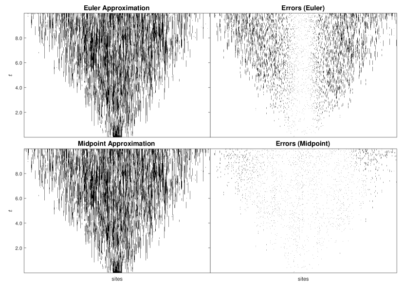
Figure 1 presents a realisation of the Euler and midpoint approximations and their evolution in time for the same spin system, coupled together with the same Poisson processes. Locations of errors from an exact Doob-Gillespie simulation for the same process are also shown. Here, the process does not start near quasi-stationarity, and the midpoint approximation displays significantly fewer errors than the Euler approximation throughout the duration of the simulation.

Refer to caption
Figure 1: Simulation of the Euler (top) and midpoint (bottom) approximations for a finite spin system with $n=2000$ sites, $q_{i}^{+}$ given by (14) with $\sigma=20$, and $q_{i}^{-}\equiv 1$ for $i=1,\dots,n$, coupled together with the same Poisson processes, and with step size $\delta=n^{-1/3}$. For each process, the realisation is presented on left with presence ($\eta_{i}(t)=1$) denoted by a black site and absence ($\eta_{i}(t)=0$) a white site. Locations of errors compared with the coupled Doob-Gillespie simulation are presented on right in black.

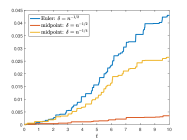
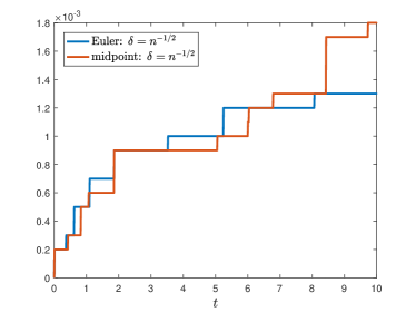
To more precisely compare the accuracy of the two methods, we can measure the largest proportion of errors encountered up to that point in time. For the Euler and midpoint approximations, this is given by

sups∈[0,t]1nβ€‹βˆ‘i=1n|Ξ·i​(s)βˆ’Ξ·iδ​(s)|,sups∈[0,t]1nβ€‹βˆ‘i=1n|Ξ·i​(s)βˆ’Ξ·ΜŠiδ​(s)|.subscriptsupremum𝑠0𝑑1𝑛superscriptsubscript𝑖1𝑛subscriptπœ‚π‘–π‘ superscriptsubscriptπœ‚π‘–π›Ώπ‘ subscriptsupremum𝑠0𝑑1𝑛superscriptsubscript𝑖1𝑛subscriptπœ‚π‘–π‘ superscriptsubscriptΜŠπœ‚π‘–π›Ώπ‘ \sup_{s\in[0,t]}\frac{1}{n}\sum_{i=1}^{n}|\eta_{i}(s)-\eta_{i}^{\delta}(s)|,\qquad\sup_{s\in[0,t]}\frac{1}{n}\sum_{i=1}^{n}|\eta_{i}(s)-\mathring{\eta}_{i}^{\delta}(s)|. (15)

These quantities are plotted in Figure 2, whose left-hand side once again illustrates the improved accuracy for the midpoint approximation when initialised away from quasi-stationarity. In fact, we see improved accuracy for the midpoint approximation, even for a much larger step size (ten times larger, in this case). On the other hand, as the process tends towards quasi-stationarity in time, $\sup_{i=1,\dots,n}\mathcal{E}_{i}(t)\to 0$. As discussed earlier, in this regime, Theorem 3.1 would still imply increased accuracy for the midpoint approximation. However, this does not appear to be the case β€” as seen in the right-hand plot of Figure 2, when the process is started near quasi-stationarity, the accuracy of the Euler and midpoint approximations appear comparable. This supports the hypothesis that the rate of convergence in Theorem 3.1 may be further improved.

Refer to caption
Refer to caption
Figure 2: Plots of the largest proportion of errors encountered (15) up to time $t$ for the Euler approximation with step size $\delta=n^{-1/2}$ (blue) and midpoint approximation with step sizes $\delta=n^{-1/2}$ (red) and $\delta=n^{-1/4}$ (yellow) for a spin system with $n=10^{4}$ sites, $q_{i}^{+}$ given by (14) with $\sigma=20$, and $q_{i}^{-}\equiv 1$ for $i=1,\dots,n$, coupled together with the same Poisson processes. The process is started with 10% of its sites initially occupied (left) and near the quasi-stationary distribution with $\mathbb{P}(\eta_{i}(0)=1)=1/2$ for all $i=1,\dots,n$ (right).

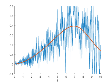
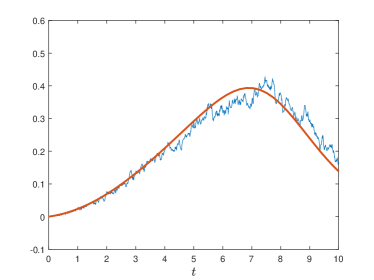
Finally, to illustrate the precision of the exact asymptotics in Theorem 3.1, Figure 3 displays the average normalised errors $(n\delta)^{-1}\sum_{i=1}^{n}(\eta_{i}(t)-\eta_{i}^{\delta}(t))$ with the average predicted errors $n^{-1}\sum_{i=1}^{n}\mathcal{E}_{i}(t)$ for the Euler approximation.

Refer to caption
Refer to caption
Figure 3: Comparison of normalised errors $(n\delta)^{-1}\sum_{i=1}^{n}(\eta_{i}(t)-\eta^{\delta}_{i}(t))$ for the Euler approximation (blue) to average predicted first-order error $n^{-1}\sum_{i=1}^{n}\mathcal{E}_{i}(t)$ (red) for a finite spin system with $q_{i}^{+}$ given by (14) with $\sigma=20$, and $q_{i}^{-}\equiv 1$ for $i=1,\dots,n$, with 10% of its sites initially occupied. The number of sites $n$ and the step size $\delta$ are taken to be $n=10^{4}$ and $\delta=n^{-1/2}$ (left); and $n=10^{5}$ and $\delta=n^{-1/4}$ (right).
Refer to caption
Figure 4: Average speedup factors for Algorithms 1 (blue) and 2 (red) over the Doob–Gillespie algorithm for the Ising–Kac model over two-dimensional site spaces of size $2^{m}\times 2^{m}$ for $m\in\{5,\dots,9\}$, with initial states $\eta_{i}(0)$ generated independently with $\mathbb{P}(\eta_{i}(0)=1)=1/2$.

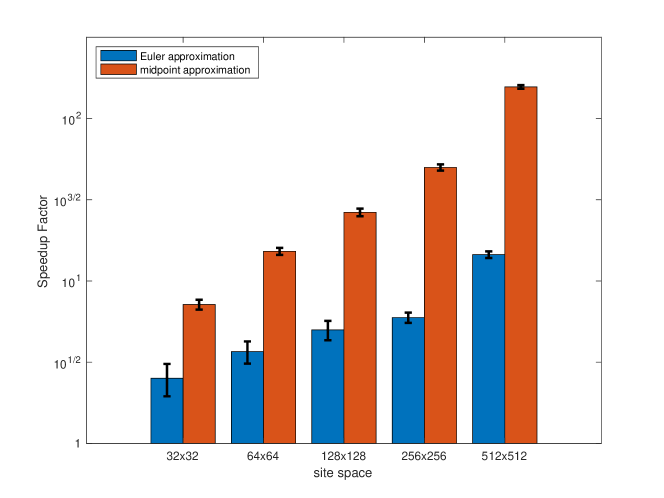
Turning now to computation time, in Figure 4, average speedup factors over the time interval $[0,T]$ for the Euler and midpoint approximations (Algorithms 1 and 2, respectively) over the Doob–Gillespie algorithm are presented. Here, we consider the Ising–Kac model over a two-dimensional site space $S=\{1,\dots,n\}\times\{1,\dots,n\}$ with $q_{i}^{+}$ and $q_{i}^{-}$ given by (12) with $\beta=1$ and $a=40n^{-1}$, which we have shown to satisfy Assumption 1. In all cases, the process is initialised with an initial distribution of $\mathbb{P}(\eta_{i}(0)=1)=1/2$. The step sizes for the Euler and midpoint approximations are chosen to be of the order of the maximal competitive step size; that is, $\delta=n^{-1/2}$ for the Euler approximation, and $\delta=n^{-1/4}$ for the midpoint approximation. As was shown in Figure 2, the accuracy of the midpoint approximation is competitive to that of the Euler approximation for these choices of step size. Despite the roughly-doubled computation time for the midpoint approximation over the Euler approximation for the same step size, for large site spaces, the significantly smaller step size for the midpoint approximation sees greatly improved performance over both the Euler and Doob-Gillespie algorithms. Altogether, Figures 2 and 4 suggest that, among the three methods discussed, the midpoint approximation is the better choice for finite spin systems not near (quasi-)stationarity. On the other hand, since the Euler approximation is universally faster to compute than the midpoint approximation for the same step size, Figure 2 suggests that the Euler approximation may be preferred for finite spin systems near (quasi-)stationarity.

Appendix A Independent site approximation

To enable the application of standard techniques, as in [4, 23], we compare $\eta(t)$ with an independent site approximation $\omega(t)$ with transition rates

$\displaystyle\omega_{i}(t)$ $\displaystyle\to\omega_{i}(t)+1\qquad\mbox{at rate }q^{+}_{i}(\rho(t))(1-\omega_{i}(t))$
$\displaystyle\omega_{i}(t)$ $\displaystyle\to\omega_{i}(t)-1\qquad\mbox{at rate }q^{-}_{i}(\rho(t))\omega_{i}(t),$

for each $i=1,\dots,n$, and where $\rho(t)$ is defined in (3). Because each element of $\omega(t)$ is independent for all time, for $1\leq r\leq 2$, using the method of bounded differences [6, Corollary 3.2] and the Lindeburg argument [23, eq. (2.5)], we can estimate for any smooth function $f$,

$$\left\lVert f(\omega(t))-f(\rho(t))\right\rVert_{r}\leq\frac{1}{2}\left(\sum_{j=1}^{n}\left\lVert\partial_{j}f\right\rVert_{\infty}^{2}\right)^{1/2}+\frac{1}{2}\sum_{j=1}^{n}\left\lVert\partial_{j}^{2}f\right\rVert_{\infty}.$$ (16)

To compare $\eta(t)$ and $\omega(t)$, we couple them together using the basic coupling for spin systems (see [27, Section III.1]). Let Ji​(T)≔supt∈[0,T]πŸ™β€‹{Ξ·i​(t)β‰ Ο‰i​(t)}≔subscript𝐽𝑖𝑇subscriptsupremum𝑑0𝑇1subscriptπœ‚π‘–π‘‘subscriptπœ”π‘–π‘‘J_{i}(T)\coloneqq\sup_{t\in[0,T]}\mathds{1}\{\eta_{i}(t)\neq\omega_{i}(t)\} and define $\bar{J}(T)\coloneqq n^{-1}\sum_{i=1}^{n}J_{i}(T)$. Now, since $\mathcal{X}=(\eta,\omega,J,\rho)$ is a Feller process, denoting by $L_{\mathcal{X}}$ the infinitesimal generator of $\mathcal{X}$, we may define the process $\mathcal{J}(t)$ by

$\displaystyle\mathcal{J}(t)$ $\displaystyle\coloneqq L_{\mathcal{X}}\bar{J}(\eta(t),\omega(t),J(t),\rho(t))$
$\displaystyle=\frac{1}{n}\sum_{i=1}^{n}L_{\mathcal{X}}J_{i}(\eta(t),\omega(t),J(t),\rho(t))$
$\displaystyle=\frac{1}{n}\sum_{i=1}^{n}(1-J_{i}(t))\{(1-\omega_{i}(t))|q^{+}_{i}(\eta(t))-q^{+}_{i}(\rho(t))|$ (17)
$\displaystyle\qquad\qquad+\omega_{i}(t)|q^{-}_{i}(\eta(t))-q^{-}_{i}(\rho(t))|\},$

and by Dynkin’s formula, since $\bar{J}(0)=0$, there exists a martingale $M$ such that

$$\bar{J}(t)=M(t)+\int_{0}^{t}\mathcal{J}(s)\mathrm{d}s,\qquad t\geq 0.$$ (18)
Lemma A.1.

For any $T\geq 0$,

$\displaystyle\mathbb{E}\bar{J}(T)$ $\displaystyle\leq n^{-1}(\|D^{\ast}q\|_{2,1}+\gamma_{n})Te^{2T\|D^{\ast}q\|_{1}}$ (19)
$\displaystyle\|\bar{J}(T)\|_{2}$ $\displaystyle\leq 2n^{-1}(1+(\|D^{\ast}q\|_{2,1}+\gamma_{n})T)e^{3T\|D^{\ast}q\|_{1}}.$ (20)
Proof.

Combining (17) and (18),

$$\frac{\mathrm{d}}{\mathrm{d}t}\mathbb{E}\bar{J}(t)=\mathbb{E}\mathcal{J}(t)\leq\frac{1}{n}\sum_{i=1}^{n}\mathbb{E}|q^{+}_{i}(\eta(t))-q^{+}_{i}(\rho(t))|+\mathbb{E}|q^{-}_{i}(\eta(t))-q^{-}_{i}(\rho(t))|,$$

and so applying (16) with the Mean Value Theorem gives

$$\mathbb{E}\mathcal{J}(t)\leq 2\|D^{\ast}q\|_{1}\mathbb{E}\bar{J}(t)+n^{-1}(\|D^{\ast}q\|_{2,1}+\gamma_{n})$$ (21)

and so

$$\mathbb{E}\bar{J}(t)\leq 2\|D^{\ast}q\|_{1}\int_{0}^{t}\mathbb{E}\bar{J}(s)\mathrm{d}s+tn^{-1}(\|D^{\ast}q\|_{2,1}+\gamma_{n}).$$

Equation (19) now follows from Gronwall’s inequality. To show (20), once again from (18),

$$\|\bar{J}(t)\|_{2}\leq\|M(t)\|_{2}+\int_{0}^{t}\|\mathcal{J}(s)\|_{2}\mathrm{d}s,\qquad t\geq 0,$$ (22)

and from (17),

$$\|\mathcal{J}(t)\|_{2}\leq\left\lVert\frac{1}{n}\sum_{i=1}^{n}q^{+}_{i}(\eta(t))-q^{+}_{i}(\rho(t))\right\rVert_{2}+\left\lVert\frac{1}{n}\sum_{i=1}^{n}q^{-}_{i}(\eta(t))-q^{-}_{i}(\rho(t))\right\rVert_{2},$$

whereby (16) with the Mean Value Theorem once again implies

$$\|\mathcal{J}(t)\|_{2}\leq 2\|D^{\ast}q\|_{1}\|\bar{J}(t)\|_{2}+n^{-1}(\|D^{\ast}q\|_{2,1}+\gamma_{n}),\qquad t\geq 0.$$ (23)

It only remains to bound $\|M(t)\|_{2}$. However, since $M(0)=0$, $\mathbb{E}M(t)^{2}=\mathbb{E}[M]_{t}$, where $[M]_{t}$ is the quadratic variation of $M$. As $\bar{J}$ moves only by jumps of size $n^{-1}$, it follows $[M]_{t}=n^{-1}\bar{J}(t)$. Therefore, by (19),

$\displaystyle\left\lVert M(T)\right\rVert_{2}$ $\displaystyle\leq n^{-1}(\|D^{\ast}q\|_{2,1}+\gamma_{n})^{1/2}T^{1/2}e^{T\|D^{\ast}q\|_{1}}$ (24)
$\displaystyle\leq n^{-1}(1+(\|D^{\ast}q\|_{2,1}+\gamma_{n})T)e^{T\|D^{\ast}q\|_{1}}.$ (25)

Combining (22), (23), and (25) yields

$$\|\bar{J}(t)\|_{2}\leq 2\|D^{\ast}q\|_{1}\int_{0}^{t}\|\bar{J}(s)\|_{2}\mathrm{d}s+2n^{-1}(1+(\|D^{\ast}q\|_{2,1}+\gamma_{n})t)e^{t\|D^{\ast}q\|_{1}},$$

from whence (20) follows by Gronwall’s inequality. ∎

Similarly, for the Euler tau-leaping process, we compare $\eta^{\delta}(t)$ with its independent site approximation $\omega^{\delta}(t)$ with transition rates

$\displaystyle\omega^{\delta}_{i}(t)$ $\displaystyle\to\omega^{\delta}_{i}(t)+1\qquad\mbox{at rate }q^{+}_{i}(\rho^{\delta}\circ\chi(t))(1-\omega^{\delta}_{i}(t))$
$\displaystyle\omega^{\delta}_{i}(t)$ $\displaystyle\to\omega^{\delta}_{i}(t)-1\qquad\mbox{at rate }q^{-}_{i}(\rho^{\delta}\circ\chi(t))\omega^{\delta}_{i}(t),$

for each $i=1,\dots,n$, where

$$\frac{d}{dt}\rho^{\delta}_{i}(t)=(1-\rho^{\delta}_{i}(t))q^{+}_{i}(\rho^{\delta}\circ\chi(t))-\rho^{\delta}_{i}(t)q^{-}_{i}(\rho^{\delta}\circ\chi(t))$$

As before, each element of $\omega^{\delta}(t)$ is independent for all time, $\mathbb{E}\omega^{\delta}(t)=\rho^{\delta}(t)$, and

$$\|f(\omega^{\delta}(t))-f(\rho^{\delta}(t))\|_{r}\leq\frac{1}{2}\left(\sum_{j=1}^{n}\|\partial_{j}f\|_{\infty}^{2}\right)^{1/2}+\frac{1}{2}\sum_{j=1}^{n}\|\partial_{j}^{2}f\|_{\infty}.$$ (26)

Define Jiδ​(T)≔supt∈[0,T]πŸ™β€‹{Ξ·iδ​(t)β‰ Ο‰iδ​(t)}≔superscriptsubscript𝐽𝑖𝛿𝑇subscriptsupremum𝑑0𝑇1subscriptsuperscriptπœ‚π›Ώπ‘–π‘‘subscriptsuperscriptπœ”π›Ώπ‘–π‘‘J_{i}^{\delta}(T)\coloneqq\sup_{t\in[0,T]}\mathds{1}\{\eta^{\delta}_{i}(t)\neq\omega^{\delta}_{i}(t)\} and $\bar{J}_{\delta}(T)\coloneqq n^{-1}\sum_{i=1}^{n}J_{i}^{\delta}(T)$. Neither $\eta^{\delta}$ nor $\omega^{\delta}$ are Markov processes, however, they are Markov over each time interval $[k\delta,(k+1)\delta)$ for $k\geq 0$. Therefore, for any $k\geq 0$, we can couple $\eta^{\delta}$ and $\omega^{\delta}$ together using the basic coupling, and form a Feller process $\mathcal{Z}_{k}=(\eta^{\delta},\omega^{\delta},J^{\delta})$ over $[k\delta,(k+1)\delta)$, conditioned on $\eta^{\delta}(k\delta)$, $\omega^{\delta}(k\delta)$, and $J^{\delta}(k\delta)$. Proceeding as before, by Dynkin’s formula, there is a martingale $M_{k}$ such that

$$\bar{J}_{\delta}(k\delta+t)=\bar{J}_{\delta}(k\delta)+M_{k}^{\delta}(t)+\int_{k\delta}^{k\delta+t}\mathcal{J}^{\delta}(s)\mathrm{d}s,\qquad 0\leq t<\delta,$$ (27)

where

$$\mathcal{J}^{\delta}(t)=\frac{1}{n}\sum_{i=1}^{n}(1-J_{i}^{\delta}(t))(1-\omega^{\delta}_{i}(t))|q^{+}_{i}(\eta^{\delta}\circ\chi(t))-q^{+}_{i}(\rho^{\delta}\circ\chi(t))|+\\ \frac{1}{n}\sum_{i=1}^{n}(1-J_{i}^{\delta}(t))\omega^{\delta}_{i}(t)|q^{-}_{i}(\eta\circ\chi(t))-q^{-}_{i}(\rho^{\delta}\circ\chi(t))|.$$
Lemma A.2.

For any $T\geq 0$,

$\displaystyle\mathbb{E}\bar{J}_{\delta}(T)$ $\displaystyle\leq n^{-1}(\|D^{\ast}q\|_{2,1}+\gamma_{n})Te^{2T\|D^{\ast}q\|_{1}}$ (28)
$\displaystyle\|\bar{J}_{\delta}(T)\|_{2}$ $\displaystyle\leq 2n^{-1}(1+(\|D^{\ast}q\|_{2,1}+\gamma_{n})T)e^{3T\|D^{\ast}q\|_{1}}.$ (29)
Proof.

As in the proof of Lemma A.1, by the Mean Value Theorem and (26),

$$\mathbb{E}\mathcal{J}^{\delta}(t)\leq 2\|D^{\ast}q\|_{1}\mathbb{E}\bar{J}_{\delta}(\chi(t))+n^{-1}(\|D^{\ast}q\|_{2,1}+\|D^{2}q\|_{1,1}),\qquad t\geq 0,$$ (30)

and so by direct integration, (27) implies that for $0\leq t<\delta$,

$$\mathbb{E}\bar{J}_{\delta}(k\delta+t)\leq(1+2t\|D^{\ast}q\|_{1})\mathbb{E}\bar{J}_{\delta}(k\delta)+tn^{-1}(\|D^{\ast}q\|_{2,1}+\gamma_{n}).$$ (31)

Since $\mathbb{E}\bar{J}_{\delta}(t)$ is continuous in $t$, taking $t\to\delta^{-}$, this implies

$$\mathbb{E}\bar{J}_{\delta}((k+1)\delta)\leq(1+2\delta\|D^{\ast}q\|_{1})\mathbb{E}\bar{J}_{\delta}(k\delta)+\delta n^{-1}(\|D^{\ast}q\|_{2,1}+\gamma_{n}).$$

Performing induction over $k$, with $\bar{J}_{\delta}(0)=0$ gives

$$\mathbb{E}\bar{J}_{\delta}(k\delta)=n^{-1}(\|D^{\ast}q\|_{2,1}+\gamma_{n})k\delta e^{2k\delta\|D^{\ast}q\|_{1}}.$$

Together with (31), this implies (28). We shall now prove (29). By iterating equation (27), for any $k\geq 0$ and $0\leq t<\delta$,

$$\bar{J}_{\delta}(k\delta+t)=\int_{0}^{k\delta+t}\mathcal{J}^{\delta}(s)\mathrm{d}s+M_{k}^{\delta}(t)+\sum_{l=0}^{k-1}M_{l}^{\delta}(\delta).$$

It can be seen that $\{M_{1}^{\delta}(\delta),\dots,M_{k-1}^{\delta}(\delta),M_{k}^{\delta}(t)\}$ forms a martingale difference sequence relative to the increasing sequence of $\sigma$-algebras $\mathcal{F}_{k}=\sigma(\eta^{\delta}(t),\omega^{\delta}(t),J^{\delta}(t),\ 0\leq t\leq k\delta)$. Therefore,

$$\left\lVert M_{k}^{\delta}(t)+\sum_{l=0}^{k-1}M_{l}^{\delta}(\delta)\right\rVert_{2}^{2}=\mathbb{E}M_{k}^{\delta}(t)^{2}+\sum_{l=0}^{k-1}\mathbb{E}M_{l}^{\delta}(\delta)^{2}.$$ (32)

Since $\mathbb{E}M_{k}^{\delta}(t)^{2}=[M_{k}^{\delta}]_{t}=n^{-1}\left(\mathbb{E}\bar{J}_{\delta}(k\delta+t)-\mathbb{E}\bar{J}_{\delta}(k\delta)\right)$ for each $k$ and $0\leq t\leq\delta$, (28) implies

$\displaystyle\left\lVert M_{k}^{\delta}(t)+\sum_{l=0}^{k-1}M_{l}^{\delta}(\delta)\right\rVert_{2}$ $\displaystyle\leq n^{-1}(\|D^{\ast}q\|_{2,1}+\gamma_{n})^{1/2}(k\delta+t)^{1/2}e^{(k\delta+t)\|D^{\ast}q\|_{1}}$
$\displaystyle\leq n^{-1}(1+(\|D^{\ast}q\|_{2,1}+\gamma_{n})(k\delta+t))e^{(k\delta+t)\|D^{\ast}q\|_{1}}.$

On the other hand, equation (26) implies that

$$\|\mathcal{J}^{\delta}(t)\|_{2}\leq 2\|D^{\ast}q\|_{1}\|\bar{J}_{\delta}(\chi(t))\|_{2}+n^{-1}(\|D^{\ast}q\|_{2,1}+\gamma_{n}),\qquad t\geq 0.$$

which altogether implies that for any $k\geq 0$ and $0\leq t<\delta$,

$$\|\bar{J}_{\delta}(k\delta+t)\|_{2}\leq 2\delta\|D^{\ast}q\|_{1}\sum_{l=0}^{k-1}\|\bar{J}_{\delta}(l\delta)\|_{2}+2t\|D^{\ast}q\|_{1}\|\bar{J}_{V}(k\delta)\|_{2}\\ +2n^{-1}(1+(\|D^{\ast}q\|_{2,1}+\gamma_{n})(k\delta+t))e^{(k\delta+t)\|D^{\ast}q\|_{1}}.$$

By induction, we find that

$$\|\bar{J}_{\delta}(k\delta)\|_{2}\leq 2n^{-1}(1+(\|D^{\ast}q\|_{2,1}+\gamma_{n})k\delta)e^{3k\delta\|D^{\ast}q\|_{1}}$$

which finally implies (29). ∎

As usual, the primary application of the independent site approximation is for obtaining a bound on the first- and second-order weak error between $\eta(t)$ and the deterministic approximation $\rho(t)$. A bound on the first-order weak error for vector-valued functions, which follows from (16), (26), and Lemmas A.1 and A.2, is presented in Lemma A.3.

Lemma A.3.

For any $f=(f_{1},\ldots,f_{m})\in\mathcal{C}^{2}([0,1]^{n},\mathbb{R}^{m})$ and any $t>0$,

$$\sum_{i=1}^{m}[\mathbb{E}\left|f_{i}(\eta(t))-f_{i}(\rho(t))\right|+\mathbb{E}|f_{i}(\eta^{\delta}(t))-f_{i}(\rho^{\delta}(t))|]\\ \leq 2\|Df\|_{1}(\|D^{\ast}q\|_{2,1}+\gamma_{n})te^{2t\|D^{\ast}q\|_{1}}+\|Df\|_{2,1}+\sum_{i,j=1}^{n}\|\partial_{j}^{2}f_{i}\|_{\infty}.$$

Following the same arguments as [23, Proposition 9], using Lemmas A.1 and A.2 in place of [23, Lemma 7], we arrive at a bound on the second-order weak error, presented in Lemma A.4. For brevity, we introduce the notation

$$\mathcal{T}_{n}(f)=\sqrt{n(1+\log n)}\left[\sqrt{n}\max_{j,k=1,\dots,n}\|\partial_{j}\partial_{k}f\|_{\infty}+\max_{j=1,\dots,n}\sum_{k=1}^{n}\|\partial_{j}\partial_{k}^{2}f\|_{\infty}\right].$$
Lemma A.4.

There is a universal constant $C>0$ such that, for any $f\in\mathcal{C}([0,1]^{n},\mathbb{R})$ and $t>0$,

$\displaystyle\mathbb{E}\left|f(\eta(t))-f(\rho(t))-\sum_{j=1}^{n}\partial_{j}f(\rho(t))(\eta_{j}(t)-\rho_{j}(t))\right|$ $\displaystyle\leq C(1+n\|\bar{J}\|_{2}^{2})\mathcal{T}_{n}(f)$
$\displaystyle\mathbb{E}\left|f(\eta^{\delta}(t))-f(\rho^{\delta}(t))-\sum_{j=1}^{n}\partial_{j}f(\rho^{\delta}(t))(\eta^{\delta}_{j}(t)-\rho^{\delta}(t))\right|$ $\displaystyle\leq C(1+n\|\bar{J}_{\delta}\|_{2}^{2})\mathcal{T}_{n}(f).$

Appendix B Proofs

B.1 Strong error analysis

We begin by providing proofs of the strong error bounds presented in Theorems 2.1 and 2.2.

Proof of Theorem 2.1.

As will be a recurring theme for all of the main results to be presented, the method of proof is centered about an application of Gronwall’s inequality. In this case, the application is fairly standard; first, by decomposing

$$\sum_{i=1}^{n}\mathbb{E}|\eta_{i}(t)-\eta_{i}^{\delta}(t)|\leq\mathbb{E}(T_{+}^{(1)}+T_{+}^{(2)}+T_{-}^{(1)}+T_{-}^{(2)}),$$

where each of the terms are given by

$\displaystyle T_{+}^{(1)}$ β‰”βˆ‘i=1n∫0t|(1βˆ’Ξ·i​(s))​qi+​(η​(s))βˆ’(1βˆ’Ξ·iδ​(s))​qi+​(ηδ​(s))|​ds≔absentsuperscriptsubscript𝑖1𝑛superscriptsubscript0𝑑1subscriptπœ‚π‘–π‘ superscriptsubscriptπ‘žπ‘–πœ‚π‘ 1subscriptsuperscriptπœ‚π›Ώπ‘–π‘ subscriptsuperscriptπ‘žπ‘–superscriptπœ‚π›Ώπ‘ differential-d𝑠\displaystyle\coloneqq\sum_{i=1}^{n}\int_{0}^{t}\left|(1-\eta_{i}(s))q_{i}^{+}(\eta(s))-(1-\eta^{\delta}_{i}(s))q^{+}_{i}(\eta^{\delta}(s))\right|\mathrm{d}s
$\displaystyle T_{+}^{(2)}$ β‰”βˆ‘i=1n∫0t|(1βˆ’Ξ·iδ​(s))​(qi+​(ηδ​(s))βˆ’qi+​(Ξ·Ξ΄βˆ˜Ο‡β€‹(s)))|​ds≔absentsuperscriptsubscript𝑖1𝑛superscriptsubscript0𝑑1subscriptsuperscriptπœ‚π›Ώπ‘–π‘ subscriptsuperscriptπ‘žπ‘–superscriptπœ‚π›Ώπ‘ subscriptsuperscriptπ‘žπ‘–superscriptπœ‚π›Ώπœ’π‘ differential-d𝑠\displaystyle\coloneqq\sum_{i=1}^{n}\int_{0}^{t}\left|(1-\eta^{\delta}_{i}(s))(q^{+}_{i}(\eta^{\delta}(s))-q^{+}_{i}(\eta^{\delta}\circ\chi(s)))\right|\mathrm{d}s
$\displaystyle T_{-}^{(1)}$ β‰”βˆ‘i=1n∫0t|Ξ·i​(s)​qiβˆ’β€‹(η​(s))βˆ’Ξ·iδ​(s)​qiβˆ’β€‹(ηδ​(s))|​ds≔absentsuperscriptsubscript𝑖1𝑛superscriptsubscript0𝑑subscriptπœ‚π‘–π‘ subscriptsuperscriptπ‘žπ‘–πœ‚π‘ subscriptsuperscriptπœ‚π›Ώπ‘–π‘ subscriptsuperscriptπ‘žπ‘–superscriptπœ‚π›Ώπ‘ differential-d𝑠\displaystyle\coloneqq\sum_{i=1}^{n}\int_{0}^{t}\left|\eta_{i}(s)q^{-}_{i}(\eta(s))-\eta^{\delta}_{i}(s)q^{-}_{i}(\eta^{\delta}(s))\right|\mathrm{d}s
$\displaystyle T_{-}^{(2)}$ β‰”βˆ‘i=1n∫0t|Ξ·iδ​(s)​(qiβˆ’β€‹(ηδ​(s))βˆ’qiβˆ’β€‹(Ξ·Ξ΄βˆ˜Ο‡β€‹(s)))|​ds.≔absentsuperscriptsubscript𝑖1𝑛superscriptsubscript0𝑑subscriptsuperscriptπœ‚π›Ώπ‘–π‘ superscriptsubscriptπ‘žπ‘–superscriptπœ‚π›Ώπ‘ superscriptsubscriptπ‘žπ‘–superscriptπœ‚π›Ώπœ’π‘ differential-d𝑠\displaystyle\coloneqq\sum_{i=1}^{n}\int_{0}^{t}\left|\eta^{\delta}_{i}(s)(q_{i}^{-}(\eta^{\delta}(s))-q_{i}^{-}(\eta^{\delta}\circ\chi(s)))\right|\mathrm{d}s.

Treating $T_{+}^{(1)}$ and $T_{+}^{(2)}$ (the arguments for $T_{-}^{(1)}$ and $T_{-}^{(2)}$ are similar), the Mean Value Theorem implies

$\displaystyle T_{+}^{(1)}$ ≀(β€–q+β€–βˆž+β€–D​q+β€–1)β€‹βˆ«0tβˆ‘i=1n|Ξ·i​(s)βˆ’Ξ·iδ​(s)|​d​s,absentsubscriptnormsuperscriptπ‘žsubscriptnorm𝐷superscriptπ‘ž1superscriptsubscript0𝑑superscriptsubscript𝑖1𝑛subscriptπœ‚π‘–π‘ subscriptsuperscriptπœ‚π›Ώπ‘–π‘ d𝑠\displaystyle\leq(\|q^{+}\|_{\infty}+\|Dq^{+}\|_{1})\int_{0}^{t}\sum_{i=1}^{n}|\eta_{i}(s)-\eta^{\delta}_{i}(s)|\mathrm{d}s,
$\displaystyle T_{+}^{(2)}$ ≀‖D​q+β€–1β€‹βˆ«0tβˆ‘i=1n|Ξ·iδ​(s)βˆ’Ξ·iΞ΄βˆ˜Ο‡β€‹(s)|​d​s.absentsubscriptnorm𝐷superscriptπ‘ž1superscriptsubscript0𝑑superscriptsubscript𝑖1𝑛subscriptsuperscriptπœ‚π›Ώπ‘–π‘ subscriptsuperscriptπœ‚π›Ώπ‘–πœ’π‘ d𝑠\displaystyle\leq\|Dq^{+}\|_{1}\int_{0}^{t}\sum_{i=1}^{n}|\eta^{\delta}_{i}(s)-\eta^{\delta}_{i}\circ\chi(s)|\mathrm{d}s.

Since |sβˆ’Ο‡β€‹(s)|β‰€Ξ΄π‘ πœ’π‘ π›Ώ|s-\chi(s)|\leq\delta for any $s\geq 0$, 𝔼​|Ξ·iδ​(s)βˆ’Ξ·iΞ΄βˆ˜Ο‡β€‹(s)|𝔼subscriptsuperscriptπœ‚π›Ώπ‘–π‘ subscriptsuperscriptπœ‚π›Ώπ‘–πœ’π‘ \mathbb{E}|\eta^{\delta}_{i}(s)-\eta^{\delta}_{i}\circ\chi(s)| is bounded above by $2\|q\|_{\infty}\delta$. Altogether, this implies

βˆ‘i=1n𝔼​|Ξ·i​(t)βˆ’Ξ·iδ​(t)|≀2​(β€–qβ€–βˆž+β€–Dβˆ—β€‹qβ€–1)β€‹βˆ«0tβˆ‘i=1n𝔼​|Ξ·i​(s)βˆ’Ξ·iδ​(s)|​d​s+4​‖qβ€–βˆžβ€‹β€–Dβˆ—β€‹qβ€–1​n​δ​t,superscriptsubscript𝑖1𝑛𝔼subscriptπœ‚π‘–π‘‘subscriptsuperscriptπœ‚π›Ώπ‘–π‘‘2subscriptdelimited-βˆ₯βˆ₯π‘žsubscriptdelimited-βˆ₯βˆ₯superscriptπ·βˆ—π‘ž1superscriptsubscript0𝑑superscriptsubscript𝑖1𝑛𝔼subscriptπœ‚π‘–π‘ subscriptsuperscriptπœ‚π›Ώπ‘–π‘ d𝑠4subscriptdelimited-βˆ₯βˆ₯π‘žsubscriptdelimited-βˆ₯βˆ₯superscriptπ·βˆ—π‘ž1𝑛𝛿𝑑\sum_{i=1}^{n}\mathbb{E}|\eta_{i}(t)-\eta^{\delta}_{i}(t)|\leq 2(\|q\|_{\infty}+\|D^{\ast}q\|_{1})\int_{0}^{t}\sum_{i=1}^{n}\mathbb{E}|\eta_{i}(s)-\eta^{\delta}_{i}(s)|\mathrm{d}s\\ +4\|q\|_{\infty}\|D^{\ast}q\|_{1}n\delta t,

and applying Gronwall’s inequality completes the proof. ∎

Proof of Theorem 2.2.

We proceed as in the proof of Theorem 2.1, but now

$\displaystyle T_{+}^{(2)}$ β‰”βˆ‘i=1n|∫0t(1βˆ’Ξ·ΜŠiδ​(s))​(qi+​(Ξ·ΜŠΞ΄β€‹(s))βˆ’qi+​(pΞ΄βˆ˜Ξ·ΜŠΞ΄βˆ˜Ο‡β€‹(s)))​ds|≔absentsuperscriptsubscript𝑖1𝑛superscriptsubscript0𝑑1subscriptsuperscriptΜŠπœ‚π›Ώπ‘–π‘ subscriptsuperscriptπ‘žπ‘–superscriptΜŠπœ‚π›Ώπ‘ subscriptsuperscriptπ‘žπ‘–superscript𝑝𝛿superscriptΜŠπœ‚π›Ώπœ’π‘ differential-d𝑠\displaystyle\coloneqq\sum_{i=1}^{n}\left|\int_{0}^{t}(1-\mathring{\eta}^{\delta}_{i}(s))(q^{+}_{i}(\mathring{\eta}^{\delta}(s))-q^{+}_{i}(p^{\delta}\circ\mathring{\eta}^{\delta}\circ\chi(s)))\mathrm{d}s\right|
$\displaystyle T_{-}^{(2)}$ β‰”βˆ‘i=1n|∫0tη̊iδ​(s)​(qiβˆ’β€‹(Ξ·ΜŠΞ΄β€‹(s))βˆ’qiβˆ’β€‹(pΞ΄βˆ˜Ξ·ΜŠΞ΄βˆ˜Ο‡β€‹(s)))​ds|.≔absentsuperscriptsubscript𝑖1𝑛superscriptsubscript0𝑑subscriptsuperscriptΜŠπœ‚π›Ώπ‘–π‘ subscriptsuperscriptπ‘žπ‘–superscriptΜŠπœ‚π›Ώπ‘ subscriptsuperscriptπ‘žπ‘–superscript𝑝𝛿superscriptΜŠπœ‚π›Ώπœ’π‘ differential-d𝑠\displaystyle\coloneqq\sum_{i=1}^{n}\left|\int_{0}^{t}\mathring{\eta}^{\delta}_{i}(s)(q^{-}_{i}(\mathring{\eta}^{\delta}(s))-q^{-}_{i}(p^{\delta}\circ\mathring{\eta}^{\delta}\circ\chi(s)))\mathrm{d}s\right|.

To apply Gronwall’s inequality as before, it is necessary to bound the expectation of these terms. In fact, it will suffice to consider $T_{+}^{(2)}$ alone, as the procedure for $T_{-}^{(2)}$ is virtually identical. Let

Ui​(s)≔qi+​(Ξ·ΜŠΞ΄β€‹(s))βˆ’qi+​(pΞ΄βˆ˜Ξ·ΜŠΞ΄βˆ˜Ο‡β€‹(s)).≔subscriptπ‘ˆπ‘–π‘ subscriptsuperscriptπ‘žπ‘–superscriptΜŠπœ‚π›Ώπ‘ subscriptsuperscriptπ‘žπ‘–superscript𝑝𝛿superscriptΜŠπœ‚π›Ώπœ’π‘ U_{i}(s)\coloneqq~{}q^{+}_{i}(\mathring{\eta}^{\delta}(s))-q^{+}_{i}(p^{\delta}\circ\mathring{\eta}^{\delta}\circ\chi(s)).

Applying a first order Taylor expansion to $q^{+}_{i}$ about Ξ·ΜŠΞ΄βˆ˜Ο‡β€‹(s)superscriptΜŠπœ‚π›Ώπœ’π‘ \mathring{\eta}^{\delta}\circ\chi(s),

Ui​(s)=βˆ‘j=1nβˆ‚jqi+​(Ξ·ΜŠΞ΄βˆ˜Ο‡β€‹(s))​(η̊jδ​(s)βˆ’Ξ·ΜŠjΞ΄βˆ˜Ο‡β€‹(s)βˆ’Ξ΄2​Qj​(Ξ·ΜŠΞ΄βˆ˜Ο‡β€‹(s)))+Ri,1+Ri,2,subscriptπ‘ˆπ‘–π‘ superscriptsubscript𝑗1𝑛subscript𝑗subscriptsuperscriptπ‘žπ‘–superscriptΜŠπœ‚π›Ώπœ’π‘ subscriptsuperscriptΜŠπœ‚π›Ώπ‘—π‘ subscriptsuperscriptΜŠπœ‚π›Ώπ‘—πœ’π‘ π›Ώ2subscript𝑄𝑗superscriptΜŠπœ‚π›Ώπœ’π‘ subscript𝑅𝑖1subscript𝑅𝑖2U_{i}(s)=\sum_{j=1}^{n}\partial_{j}q^{+}_{i}(\mathring{\eta}^{\delta}\circ\chi(s))\left(\mathring{\eta}^{\delta}_{j}(s)-\mathring{\eta}^{\delta}_{j}\circ\chi(s)-\frac{\delta}{2}Q_{j}(\mathring{\eta}^{\delta}\circ\chi(s))\right)\\ +R_{i,1}+R_{i,2},

where $R_{i,1}$ and $R_{i,2}$ are the remainders from the expansion of qi+​(pΞ΄βˆ˜Ξ·ΜŠΞ΄βˆ˜Ο‡β€‹(s))subscriptsuperscriptπ‘žπ‘–superscript𝑝𝛿superscriptΜŠπœ‚π›Ώπœ’π‘ q^{+}_{i}(p^{\delta}\circ\mathring{\eta}^{\delta}\circ\chi(s)) and qi+​(Ξ·ΜŠΞ΄β€‹(s))subscriptsuperscriptπ‘žπ‘–superscriptΜŠπœ‚π›Ώπ‘ q^{+}_{i}(\mathring{\eta}^{\delta}(s)), respectively. Note that $|R_{i,1}|\leq\delta^{2}\|q\|_{\infty}^{2}\sum_{j,k=1}^{n}\|\partial_{j}\partial_{k}q^{+}_{i}\|_{\infty}$. For $R_{i,2}$,

$\displaystyle\mathbb{E}\left|R_{i,2}\right|$ β‰€βˆ‘j,k=1nβ€–βˆ‚jβˆ‚kqi+β€–βˆžβ€‹π”Όβ€‹|(η̊jδ​(s)βˆ’Ξ·ΜŠjΞ΄βˆ˜Ο‡β€‹(s))​(η̊kδ​(s)βˆ’Ξ·ΜŠkΞ΄βˆ˜Ο‡β€‹(s))|.absentsuperscriptsubscriptπ‘—π‘˜1𝑛subscriptnormsubscript𝑗subscriptπ‘˜subscriptsuperscriptπ‘žπ‘–π”ΌsubscriptsuperscriptΜŠπœ‚π›Ώπ‘—π‘ subscriptsuperscriptΜŠπœ‚π›Ώπ‘—πœ’π‘ subscriptsuperscriptΜŠπœ‚π›Ώπ‘˜π‘ subscriptsuperscriptΜŠπœ‚π›Ώπ‘˜πœ’π‘ \displaystyle\leq\sum_{j,k=1}^{n}\|\partial_{j}\partial_{k}q^{+}_{i}\|_{\infty}\mathbb{E}\left|(\mathring{\eta}^{\delta}_{j}(s)-\mathring{\eta}^{\delta}_{j}\circ\chi(s))(\mathring{\eta}^{\delta}_{k}(s)-\mathring{\eta}^{\delta}_{k}\circ\chi(s))\right|.

From (7), the number of jumps in $\mathring{\eta}^{\delta}_{i}$ on $[a,b]$ is stochastically dominated by a Poisson random variable with mean $2\|q\|_{\infty}(b-a)$ so for each $j=1,\dots,n$,

𝔼​[|η̊jδ​(s)βˆ’Ξ·ΜŠjΞ΄βˆ˜Ο‡β€‹(s)||Ξ·ΜŠΞ΄βˆ˜Ο‡β€‹(s)]≀1βˆ’eβˆ’2​δ​‖qβ€–βˆžβ‰€2​δ​‖qβ€–βˆž.𝔼delimited-[]conditionalsubscriptsuperscriptΜŠπœ‚π›Ώπ‘—π‘ subscriptsuperscriptΜŠπœ‚π›Ώπ‘—πœ’π‘ superscriptΜŠπœ‚π›Ώπœ’π‘ 1superscript𝑒2𝛿subscriptnormπ‘ž2𝛿subscriptnormπ‘ž\mathbb{E}\left[\left.|\mathring{\eta}^{\delta}_{j}(s)-\mathring{\eta}^{\delta}_{j}\circ\chi(s)|\;\right|\;\mathring{\eta}^{\delta}\circ\chi(s)\right]\leq 1-e^{-2\delta\|q\|_{\infty}}\leq 2\delta\|q\|_{\infty}.

Since the η̊jδ​(s)subscriptsuperscriptΜŠπœ‚π›Ώπ‘—π‘ \mathring{\eta}^{\delta}_{j}(s) are independent conditioned on Ξ·ΜŠΞ΄βˆ˜Ο‡β€‹(s)superscriptΜŠπœ‚π›Ώπœ’π‘ \mathring{\eta}^{\delta}\circ\chi(s), it follows

$\displaystyle\mathbb{E}\left|R_{i,2}\right|$ ≀4​δ2​‖qβ€–βˆž2β€‹βˆ‘j,k=1jβ‰ knβ€–βˆ‚jβˆ‚kqi+β€–βˆž+2​δ​‖qβ€–βˆžβ€‹βˆ‘j=1nβ€–βˆ‚j2qi+β€–βˆž.absent4superscript𝛿2superscriptsubscriptnormπ‘ž2superscriptsubscriptπ‘—π‘˜1π‘—π‘˜π‘›subscriptnormsubscript𝑗subscriptπ‘˜subscriptsuperscriptπ‘žπ‘–2𝛿subscriptnormπ‘žsuperscriptsubscript𝑗1𝑛subscriptnormsuperscriptsubscript𝑗2subscriptsuperscriptπ‘žπ‘–\displaystyle\leq 4\delta^{2}\|q\|_{\infty}^{2}\sum_{\begin{subarray}{c}j,k=1\\ j\neq k\end{subarray}}^{n}\|\partial_{j}\partial_{k}q^{+}_{i}\|_{\infty}+2\delta\|q\|_{\infty}\sum_{j=1}^{n}\|\partial_{j}^{2}q^{+}_{i}\|_{\infty}.

For each $i=1,\dots,n$, define

U~i​(s)≔(sβˆ’Ο‡β€‹(s)βˆ’Ξ΄2)β€‹βˆ‘j=1nβˆ‚jqi+​(Ξ·ΜŠΞ΄βˆ˜Ο‡β€‹(s))​qj​(Ξ·ΜŠΞ΄βˆ˜Ο‡β€‹(s)).≔subscript~π‘ˆπ‘–π‘ π‘ πœ’π‘ π›Ώ2superscriptsubscript𝑗1𝑛subscript𝑗subscriptsuperscriptπ‘žπ‘–superscriptΜŠπœ‚π›Ώπœ’π‘ subscriptπ‘žπ‘—superscriptΜŠπœ‚π›Ώπœ’π‘ \tilde{U}_{i}(s)\coloneqq\left(s-\chi(s)-\frac{\delta}{2}\right)\sum_{j=1}^{n}\partial_{j}q^{+}_{i}(\mathring{\eta}^{\delta}\circ\chi(s))q_{j}(\mathring{\eta}^{\delta}\circ\chi(s)).

Since βˆ«Ο‡β€‹(t)χ​(t)+Ξ΄|sβˆ’Ο‡β€‹(s)βˆ’Ξ΄/2|​ds=Ξ΄2/4subscriptsuperscriptπœ’π‘‘π›Ώπœ’π‘‘π‘ πœ’π‘ π›Ώ2differential-d𝑠superscript𝛿24\int^{\chi(t)+\delta}_{\chi(t)}|s-\chi(s)-\delta/2|\mathrm{d}s=\delta^{2}/4 and βˆ«Ο‡β€‹(t)χ​(t)+Ξ΄(sβˆ’Ο‡β€‹(s)βˆ’Ξ΄/2)​ds=0subscriptsuperscriptπœ’π‘‘π›Ώπœ’π‘‘π‘ πœ’π‘ π›Ώ2differential-d𝑠0\int^{\chi(t)+\delta}_{\chi(t)}(s-\chi(s)-\delta/2)\mathrm{d}s=0 for any bounded function $g$ and any $t>0$,

|∫0t(1βˆ’Ξ·ΜŠiδ​(s))​(sβˆ’Ο‡β€‹(s)βˆ’Ξ΄2)​g​(χ​(s))​ds|≀δ2​‖gβ€–βˆžβ€‹(1+βˆ‘s∈[0,t]Ξ”β€‹Ξ·ΜŠiδ​(s)).subscriptsuperscript𝑑01subscriptsuperscriptΜŠπœ‚π›Ώπ‘–π‘ π‘ πœ’π‘ π›Ώ2π‘”πœ’π‘ differential-d𝑠superscript𝛿2subscriptnorm𝑔1subscript𝑠0𝑑ΔsubscriptsuperscriptΜŠπœ‚π›Ώπ‘–π‘ \left|\int^{t}_{0}(1-\mathring{\eta}^{\delta}_{i}(s))\left(s-\chi(s)-\frac{\delta}{2}\right)g(\chi(s))\mathrm{d}s\right|\leq\delta^{2}\|g\|_{\infty}\left(1+\sum_{s\in[0,t]}\Delta\mathring{\eta}^{\delta}_{i}(s)\right).

Again using the fact that the expected number of jumps in $\mathring{\eta}^{\delta}_{i}$ on $[a,b]$ is bounded by $2\|q\|_{\infty}(b-a)$,

𝔼​|∫0t(1βˆ’Ξ·ΜŠiδ​(s))​U~i​(s)​ds|≀2​(t+1)​δ2​‖qβ€–βˆžβ€‹(1+β€–qβ€–βˆž)β€‹βˆ‘j=1nβ€–βˆ‚jqi+β€–βˆž.𝔼subscriptsuperscript𝑑01subscriptsuperscriptΜŠπœ‚π›Ώπ‘–π‘ subscript~π‘ˆπ‘–π‘ differential-d𝑠2𝑑1superscript𝛿2subscriptnormπ‘ž1subscriptnormπ‘žsuperscriptsubscript𝑗1𝑛subscriptnormsubscript𝑗subscriptsuperscriptπ‘žπ‘–\displaystyle\mathbb{E}\left|\int^{t}_{0}(1-\mathring{\eta}^{\delta}_{i}(s))\tilde{U}_{i}(s)\mathrm{d}s\right|\leq 2(t+1)\delta^{2}\|q\|_{\infty}(1+\|q\|_{\infty})\sum_{j=1}^{n}\|\partial_{j}q^{+}_{i}\|_{\infty}. (33)

Therefore, to control $T_{+}^{(2)}$, it now suffices to consider the remaining error term

𝔼​|∫0t(1βˆ’Ξ·ΜŠiδ​(s))​(Ui​(s)βˆ’U~i​(s))​ds|≀t​sups∈[0,t]𝔼​|Ui​(s)βˆ’U~i​(s)|.𝔼subscriptsuperscript𝑑01subscriptsuperscriptΜŠπœ‚π›Ώπ‘–π‘ subscriptπ‘ˆπ‘–π‘ subscript~π‘ˆπ‘–π‘ differential-d𝑠𝑑subscriptsupremum𝑠0𝑑𝔼subscriptπ‘ˆπ‘–π‘ subscript~π‘ˆπ‘–π‘ \mathbb{E}\left|\int^{t}_{0}(1-\mathring{\eta}^{\delta}_{i}(s))(U_{i}(s)-\tilde{U}_{i}(s))\mathrm{d}s\right|\leq t\sup_{s\in[0,t]}\mathbb{E}|U_{i}(s)-\tilde{U}_{i}(s)|.

To do so, let $M(t)$ denote the martingale

Mi(t)=η̊iΞ΄(t)βˆ’βˆ«0t((1βˆ’Ξ·ΜŠiΞ΄(s))qi+(pΞ΄βˆ˜Ξ·ΜŠΞ΄βˆ˜Ο‡(s))βˆ’Ξ·ΜŠiΞ΄(s)qiβˆ’(pΞ΄βˆ˜Ξ·ΜŠΞ΄βˆ˜Ο‡(s)))ds.subscript𝑀𝑖𝑑subscriptsuperscriptΜŠπœ‚π›Ώπ‘–π‘‘subscriptsuperscript𝑑01subscriptsuperscriptΜŠπœ‚π›Ώπ‘–π‘ subscriptsuperscriptπ‘žπ‘–superscript𝑝𝛿superscriptΜŠπœ‚π›Ώπœ’π‘ subscriptsuperscriptΜŠπœ‚π›Ώπ‘–π‘ subscriptsuperscriptπ‘žπ‘–superscript𝑝𝛿superscriptΜŠπœ‚π›Ώπœ’π‘ d𝑠M_{i}(t)=\mathring{\eta}^{\delta}_{i}(t)-\int^{t}_{0}((1-\mathring{\eta}^{\delta}_{i}(s))q^{+}_{i}(p^{\delta}\circ\mathring{\eta}^{\delta}\circ\chi(s))\\ -\mathring{\eta}^{\delta}_{i}(s)q^{-}_{i}(p^{\delta}\circ\mathring{\eta}^{\delta}\circ\chi(s)))\mathrm{d}s.

In terms of $M(t)$, the difference Ui​(s)βˆ’U~i​(s)=Ti,1+Ti,2βˆ’Ti,3βˆ’Ti,4+Ri,1+Ri,2subscriptπ‘ˆπ‘–π‘ subscript~π‘ˆπ‘–π‘ subscript𝑇𝑖1subscript𝑇𝑖2subscript𝑇𝑖3subscript𝑇𝑖4subscript𝑅𝑖1subscript𝑅𝑖2U_{i}(s)-\tilde{U}_{i}(s)=T_{i,1}+T_{i,2}-T_{i,3}-T_{i,4}+R_{i,1}+R_{i,2}, where

$\displaystyle T_{i,1}$ =βˆ‘j=1nβˆ‚jqi+​(Ξ·ΜŠΞ΄βˆ˜Ο‡β€‹(s))​(Mj​(s)βˆ’Mjβˆ˜Ο‡β€‹(s))absentsuperscriptsubscript𝑗1𝑛subscript𝑗subscriptsuperscriptπ‘žπ‘–superscriptΜŠπœ‚π›Ώπœ’π‘ subscript𝑀𝑗𝑠subscriptπ‘€π‘—πœ’π‘ \displaystyle=\sum_{j=1}^{n}\partial_{j}q^{+}_{i}(\mathring{\eta}^{\delta}\circ\chi(s))(M_{j}(s)-M_{j}\circ\chi(s))
$\displaystyle T_{i,2}$ =βˆ‘j=1nβˆ‚jqi+​(Ξ·ΜŠΞ΄βˆ˜Ο‡β€‹(s))β€‹βˆ«Ο‡β€‹(s)s(1βˆ’Ξ·ΜŠjδ​(u))​[qj+​(pΞ΄βˆ˜Ξ·ΜŠΞ΄βˆ˜Ο‡β€‹(u))βˆ’qj+​(Ξ·ΜŠΞ΄βˆ˜Ο‡β€‹(u))]​duabsentsuperscriptsubscript𝑗1𝑛subscript𝑗subscriptsuperscriptπ‘žπ‘–superscriptΜŠπœ‚π›Ώπœ’π‘ subscriptsuperscriptπ‘ πœ’π‘ 1subscriptsuperscriptΜŠπœ‚π›Ώπ‘—π‘’delimited-[]subscriptsuperscriptπ‘žπ‘—superscript𝑝𝛿superscriptΜŠπœ‚π›Ώπœ’π‘’subscriptsuperscriptπ‘žπ‘—superscriptΜŠπœ‚π›Ώπœ’π‘’differential-d𝑒\displaystyle=\sum_{j=1}^{n}\partial_{j}q^{+}_{i}(\mathring{\eta}^{\delta}\circ\chi(s))\int^{s}_{\chi(s)}(1-\mathring{\eta}^{\delta}_{j}(u))\left[q^{+}_{j}(p^{\delta}\circ\mathring{\eta}^{\delta}\circ\chi(u))-q^{+}_{j}(\mathring{\eta}^{\delta}\circ\chi(u))\right]\mathrm{d}u
$\displaystyle T_{i,3}$ =βˆ‘j=1nβˆ‚jqi+​(Ξ·ΜŠΞ΄βˆ˜Ο‡β€‹(s))β€‹βˆ«Ο‡β€‹(s)sη̊jδ​(u)​[qjβˆ’β€‹(pΞ΄βˆ˜Ξ·ΜŠΞ΄βˆ˜Ο‡β€‹(u))βˆ’qjβˆ’β€‹(Ξ·ΜŠΞ΄βˆ˜Ο‡β€‹(u))]​duabsentsuperscriptsubscript𝑗1𝑛subscript𝑗subscriptsuperscriptπ‘žπ‘–superscriptΜŠπœ‚π›Ώπœ’π‘ subscriptsuperscriptπ‘ πœ’π‘ subscriptsuperscriptΜŠπœ‚π›Ώπ‘—π‘’delimited-[]subscriptsuperscriptπ‘žπ‘—superscript𝑝𝛿superscriptΜŠπœ‚π›Ώπœ’π‘’subscriptsuperscriptπ‘žπ‘—superscriptΜŠπœ‚π›Ώπœ’π‘’differential-d𝑒\displaystyle=\sum_{j=1}^{n}\partial_{j}q^{+}_{i}(\mathring{\eta}^{\delta}\circ\chi(s))\int^{s}_{\chi(s)}\mathring{\eta}^{\delta}_{j}(u)\left[q^{-}_{j}(p^{\delta}\circ\mathring{\eta}^{\delta}\circ\chi(u))-q^{-}_{j}(\mathring{\eta}^{\delta}\circ\chi(u))\right]\mathrm{d}u
$\displaystyle T_{i,4}$ =βˆ‘j=1nβˆ‚jqi+​(Ξ·ΜŠΞ΄βˆ˜Ο‡β€‹(s))​[qj+​(Ξ·ΜŠΞ΄βˆ˜Ο‡β€‹(s))+qjβˆ’β€‹(Ξ·ΜŠΞ΄βˆ˜Ο‡β€‹(s))]β€‹βˆ«Ο‡β€‹(s)s[η̊jδ​(u)βˆ’Ξ·ΜŠjΞ΄βˆ˜Ο‡β€‹(u)]​du.absentsuperscriptsubscript𝑗1𝑛subscript𝑗subscriptsuperscriptπ‘žπ‘–superscriptΜŠπœ‚π›Ώπœ’π‘ delimited-[]subscriptsuperscriptπ‘žπ‘—superscriptΜŠπœ‚π›Ώπœ’π‘ subscriptsuperscriptπ‘žπ‘—superscriptΜŠπœ‚π›Ώπœ’π‘ superscriptsubscriptπœ’π‘ π‘ delimited-[]subscriptsuperscriptΜŠπœ‚π›Ώπ‘—π‘’subscriptsuperscriptΜŠπœ‚π›Ώπ‘—πœ’π‘’differential-d𝑒\displaystyle=\sum_{j=1}^{n}\partial_{j}q^{+}_{i}(\mathring{\eta}^{\delta}\circ\chi(s))[q^{+}_{j}(\mathring{\eta}^{\delta}\circ\chi(s))+q^{-}_{j}(\mathring{\eta}^{\delta}\circ\chi(s))]\int_{\chi(s)}^{s}[\mathring{\eta}^{\delta}_{j}(u)-\mathring{\eta}^{\delta}_{j}\circ\chi(u)]\mathrm{d}u.

First, to bound $T_{i,1}$, let Mi+​(s)β‰”βˆ‘j=1nβˆ‚jqi+​(Ξ·ΜŠΞ΄βˆ˜Ο‡β€‹(s))​Mj​(s)≔subscriptsuperscript𝑀𝑖𝑠superscriptsubscript𝑗1𝑛subscript𝑗subscriptsuperscriptπ‘žπ‘–superscriptΜŠπœ‚π›Ώπœ’π‘ subscript𝑀𝑗𝑠M^{+}_{i}(s)\coloneqq\sum_{j=1}^{n}\partial_{j}q^{+}_{i}(\mathring{\eta}^{\delta}\circ\chi(s))M_{j}(s), so that

𝔼​Ti,12=𝔼​[Mi+​(s)βˆ’Mi+βˆ˜Ο‡β€‹(s)]2=𝔼​[Mi+]sβˆ’π”Όβ€‹[Mi+]χ​(s).𝔼superscriptsubscript𝑇𝑖12𝔼superscriptdelimited-[]subscriptsuperscript𝑀𝑖𝑠subscriptsuperscriptπ‘€π‘–πœ’π‘ 2𝔼subscriptdelimited-[]subscriptsuperscript𝑀𝑖𝑠𝔼subscriptdelimited-[]subscriptsuperscriptπ‘€π‘–πœ’π‘ \mathbb{E}T_{i,1}^{2}=\mathbb{E}[M^{+}_{i}(s)-M^{+}_{i}\circ\chi(s)]^{2}=\mathbb{E}[M^{+}_{i}]_{s}-\mathbb{E}[M^{+}_{i}]_{\chi(s)}.

Note that the quadratic variation of $M_{j}$, (resp. $M^{+}_{i}$), is just the number of jumps in $M_{j}$ (resp. $M^{+}_{i}$) and that, recalling the defining property of a spin system, with probability one, no two sites experience simultaneous jumps in $\mathring{\eta}^{\delta}$. Therefore, 𝔼​[Mi+]sβˆ’π”Όβ€‹[Mi+]χ​(s)≀2​δ​‖qβ€–βˆžβ€‹βˆ‘j=1nβ€–βˆ‚jqi+β€–βˆž2𝔼subscriptdelimited-[]subscriptsuperscript𝑀𝑖𝑠𝔼subscriptdelimited-[]subscriptsuperscriptπ‘€π‘–πœ’π‘ 2𝛿subscriptnormπ‘žsuperscriptsubscript𝑗1𝑛superscriptsubscriptnormsubscript𝑗subscriptsuperscriptπ‘žπ‘–2\mathbb{E}[M^{+}_{i}]_{s}-\mathbb{E}[M^{+}_{i}]_{\chi(s)}\leq 2\delta\|q\|_{\infty}\sum_{j=1}^{n}\|\partial_{j}q^{+}_{i}\|_{\infty}^{2}, and so

$$(\mathbb{E}|T_{i,1}|)^{2}\leq 2\delta\|q\|_{\infty}\sum_{j=1}^{n}\|\partial_{j}q^{+}_{i}\|_{\infty}^{2}.$$ (34)

The terms $T_{i,2}$ and $T_{i,3}$ are controlled together: by the Mean Value Theorem,

|qj+​(pΞ΄βˆ˜Ξ·ΜŠΞ΄βˆ˜Ο‡β€‹(s))βˆ’qj+​(Ξ·ΜŠΞ΄βˆ˜Ο‡β€‹(s))|subscriptsuperscriptπ‘žπ‘—superscript𝑝𝛿superscriptΜŠπœ‚π›Ώπœ’π‘ subscriptsuperscriptπ‘žπ‘—superscriptΜŠπœ‚π›Ώπœ’π‘ \displaystyle|q^{+}_{j}(p^{\delta}\circ\mathring{\eta}^{\delta}\circ\chi(s))-q^{+}_{j}(\mathring{\eta}^{\delta}\circ\chi(s))| $\displaystyle\leq\frac{1}{2}\delta\|q\|_{\infty}\sum_{k=1}^{n}\|\partial_{k}q^{+}_{j}\|_{\infty},$

and similarly for $q_{j}^{-}$, which implies

$\displaystyle\mathbb{E}|T_{i,2}|+\mathbb{E}|T_{i,3}|$ $\displaystyle\leq\frac{1}{2}\delta^{2}\|q\|_{\infty}\sum_{j,k=1}^{n}\|\partial_{j}q^{+}_{i}\|_{\infty}\left(\|\partial_{k}q^{+}_{j}\|_{\infty}+\|\partial_{k}q^{-}_{j}\|_{\infty}\right).$ (35)

Finally, to bound $T_{i,4}$,

$\displaystyle\mathbb{E}|T_{i,4}|$ ≀2​‖qβ€–βˆžβ€‹βˆ‘j=1nβ€–βˆ‚jqi+β€–βˆžβ€‹βˆ«Ο‡β€‹(s)s𝔼​|η̊jδ​(u)βˆ’Ξ·ΜŠjΞ΄βˆ˜Ο‡β€‹(u)|​duabsent2subscriptnormπ‘žsuperscriptsubscript𝑗1𝑛subscriptnormsubscript𝑗subscriptsuperscriptπ‘žπ‘–subscriptsuperscriptπ‘ πœ’π‘ π”ΌsubscriptsuperscriptΜŠπœ‚π›Ώπ‘—π‘’subscriptsuperscriptΜŠπœ‚π›Ώπ‘—πœ’π‘’differential-d𝑒\displaystyle\leq 2\|q\|_{\infty}\sum_{j=1}^{n}\|\partial_{j}q^{+}_{i}\|_{\infty}\int^{s}_{\chi(s)}\mathbb{E}|\mathring{\eta}^{\delta}_{j}(u)-\mathring{\eta}^{\delta}_{j}\circ\chi(u)|\mathrm{d}u
≀2​δ​‖qβ€–βˆžβ€‹βˆ‘j=1nβ€–βˆ‚jqi+β€–βˆžβ€‹π”Όβ€‹βˆ‘u∈[χ​(s),s]Ξ”β€‹Ξ·ΜŠjδ​(u)≀4​δ2​‖qβ€–βˆž2β€‹βˆ‘j=1nβ€–βˆ‚jqi+β€–βˆž.absent2𝛿subscriptnormπ‘žsuperscriptsubscript𝑗1𝑛subscriptnormsubscript𝑗subscriptsuperscriptπ‘žπ‘–π”Όsubscriptπ‘’πœ’π‘ π‘ Ξ”subscriptsuperscriptΜŠπœ‚π›Ώπ‘—π‘’4superscript𝛿2subscriptsuperscriptnormπ‘ž2superscriptsubscript𝑗1𝑛subscriptnormsubscript𝑗subscriptsuperscriptπ‘žπ‘–\displaystyle\leq 2\delta\|q\|_{\infty}\sum_{j=1}^{n}\|\partial_{j}q^{+}_{i}\|_{\infty}\ \mathbb{E}\sum_{u\in[\chi(s),s]}\Delta\mathring{\eta}^{\delta}_{j}(u)\leq 4\delta^{2}\|q\|^{2}_{\infty}\sum_{j=1}^{n}\|\partial_{j}q^{+}_{i}\|_{\infty}. (36)

Combining (33)-(36) with the bounds on $R_{i,1}$ and $R_{i,2}$ gives

$$\mathbb{E}|T_{+}^{(2)}|\leq 5(t+1)n\delta^{2}\|q\|_{\infty}(1+\|q\|_{\infty})[\|D^{\ast}q\|_{1}+\Gamma_{n}+\|D^{\ast}q\|_{1}^{2}]\\ +2\delta t\|q\|_{\infty}\gamma_{n}+\sqrt{2}\delta^{1/2}\|q\|_{\infty}^{1/2}t\|D^{\ast}q\|_{2,1}$$

and so $\mathbb{E}|T_{+}^{(2)}|\leq 5\alpha(n,\delta)(1+t)$. Applying the same arguments to $T^{(2)}_{-}$ yields

βˆ‘i=1n𝔼​|Ξ·i​(t)βˆ’Ξ·ΜŠiδ​(t)|≀2​(β€–qβ€–βˆž+β€–Dβˆ—β€‹qβ€–1)β€‹βˆ«0tβˆ‘i=1n𝔼​|Ξ·i​(s)βˆ’Ξ·ΜŠiδ​(s)|​d​s+10​α​(n,Ξ΄)​(1+t).superscriptsubscript𝑖1𝑛𝔼subscriptπœ‚π‘–π‘‘subscriptsuperscriptΜŠπœ‚π›Ώπ‘–π‘‘2subscriptdelimited-βˆ₯βˆ₯π‘žsubscriptdelimited-βˆ₯βˆ₯superscriptπ·βˆ—π‘ž1superscriptsubscript0𝑑superscriptsubscript𝑖1𝑛𝔼subscriptπœ‚π‘–π‘ subscriptsuperscriptΜŠπœ‚π›Ώπ‘–π‘ d𝑠10𝛼𝑛𝛿1𝑑\sum_{i=1}^{n}\mathbb{E}|\eta_{i}(t)-\mathring{\eta}^{\delta}_{i}(t)|\leq 2(\|q\|_{\infty}+\|D^{\ast}q\|_{1})\int_{0}^{t}\sum_{i=1}^{n}\mathbb{E}|\eta_{i}(s)-\mathring{\eta}^{\delta}_{i}(s)|\mathrm{d}s\\ +10\alpha(n,\delta)(1+t).

The proof is completed by applying Gronwall’s inequality as in the proof of Theorem 2.1. ∎

B.2 Proof of Theorem 3.1

Throughout this proof, for the sake of brevity, the notation $x\lesssim y$ will be used to imply there exists some universal constant $c>0$ such that $x\leq cy$. Naturally, we assume throughout that the hypotheses of Theorem 3.1 hold. We begin by coupling $\eta(t)$ and $\eta^{\delta}(t)$ using the basic coupling, that is, for independent unit-rate Poisson processes $N_{i,k}^{+},N_{i,k}^{-}$ with $i=1,\dots,n;\ k=1,2,3$:

$\displaystyle\eta_{i}(t)$ $\displaystyle=\eta_{i}(0)+N_{i,1}^{+}\left(\int^{t}_{0}[(1-\eta_{i}(s))q^{+}_{i}(\eta(s))\wedge(1-\eta^{\delta}_{i}(s)q^{+}_{i}(\eta^{\delta}\circ\chi(s))]\mathrm{d}s\right)$
+Ni,2+​(∫0t[(1βˆ’Ξ·i​(s))​qi+​(η​(s))βˆ’(1βˆ’Ξ·iδ​(s))​qi+​(Ξ·Ξ΄βˆ˜Ο‡β€‹(s))]+​ds)superscriptsubscript𝑁𝑖2subscriptsuperscript𝑑0subscriptdelimited-[]1subscriptπœ‚π‘–π‘ subscriptsuperscriptπ‘žπ‘–πœ‚π‘ 1subscriptsuperscriptπœ‚π›Ώπ‘–π‘ subscriptsuperscriptπ‘žπ‘–superscriptπœ‚π›Ώπœ’π‘ differential-d𝑠\displaystyle+N_{i,2}^{+}\left(\int^{t}_{0}[(1-\eta_{i}(s))q^{+}_{i}(\eta(s))-(1-\eta^{\delta}_{i}(s))q^{+}_{i}(\eta^{\delta}\circ\chi(s))]_{+}\mathrm{d}s\right)
βˆ’Ni,1βˆ’β€‹(∫0t[Ξ·i​(s)​qiβˆ’β€‹(η​(s))∧ηiδ​(s)​qiβˆ’β€‹(Ξ·Ξ΄βˆ˜Ο‡β€‹(s))]​ds)superscriptsubscript𝑁𝑖1subscriptsuperscript𝑑0delimited-[]subscriptπœ‚π‘–π‘ subscriptsuperscriptπ‘žπ‘–πœ‚π‘ subscriptsuperscriptπœ‚π›Ώπ‘–π‘ subscriptsuperscriptπ‘žπ‘–superscriptπœ‚π›Ώπœ’π‘ differential-d𝑠\displaystyle-N_{i,1}^{-}\left(\int^{t}_{0}[\eta_{i}(s)q^{-}_{i}(\eta(s))\wedge\eta^{\delta}_{i}(s)q^{-}_{i}(\eta^{\delta}\circ\chi(s))]\mathrm{d}s\right)
βˆ’Ni,2βˆ’β€‹(∫0t[Ξ·i​(s)​qiβˆ’β€‹(η​(s))βˆ’Ξ·iδ​(s)​qiβˆ’β€‹(Ξ·Ξ΄βˆ˜Ο‡β€‹(s))]+​ds)superscriptsubscript𝑁𝑖2subscriptsuperscript𝑑0subscriptdelimited-[]subscriptπœ‚π‘–π‘ subscriptsuperscriptπ‘žπ‘–πœ‚π‘ subscriptsuperscriptπœ‚π›Ώπ‘–π‘ subscriptsuperscriptπ‘žπ‘–superscriptπœ‚π›Ώπœ’π‘ differential-d𝑠\displaystyle-N_{i,2}^{-}\left(\int^{t}_{0}[\eta_{i}(s)q^{-}_{i}(\eta(s))-\eta^{\delta}_{i}(s)q^{-}_{i}(\eta^{\delta}\circ\chi(s))]_{+}\mathrm{d}s\right)

and

$\displaystyle\eta^{\delta}_{i}(t)$ $\displaystyle=\eta_{i}(0)+N_{i,1}^{+}\left(\int^{t}_{0}\left[(1-\eta_{i}(s))q^{+}_{i}(\eta(s))\wedge(1-\eta^{\delta}_{i}(s)q^{+}_{i}(\eta^{\delta}\circ\chi(s))\right]\mathrm{d}s\right)$
+Ni,3+​(∫0t[(1βˆ’Ξ·iδ​(s))​qi+​(Ξ·Ξ΄βˆ˜Ο‡β€‹(s))βˆ’(1βˆ’Ξ·i​(s))​qi+​(η​(s))]+​ds)superscriptsubscript𝑁𝑖3subscriptsuperscript𝑑0subscriptdelimited-[]1subscriptsuperscriptπœ‚π›Ώπ‘–π‘ subscriptsuperscriptπ‘žπ‘–superscriptπœ‚π›Ώπœ’π‘ 1subscriptπœ‚π‘–π‘ subscriptsuperscriptπ‘žπ‘–πœ‚π‘ differential-d𝑠\displaystyle+N_{i,3}^{+}\left(\int^{t}_{0}[(1-\eta^{\delta}_{i}(s))q^{+}_{i}(\eta^{\delta}\circ\chi(s))-(1-\eta_{i}(s))q^{+}_{i}(\eta(s))]_{+}\mathrm{d}s\right)
βˆ’Ni,1βˆ’β€‹(∫0t[Ξ·i​(s)​qiβˆ’β€‹(η​(s))∧ηiδ​(s)​qiβˆ’β€‹(Ξ·Ξ΄βˆ˜Ο‡β€‹(s))]​ds)superscriptsubscript𝑁𝑖1subscriptsuperscript𝑑0delimited-[]subscriptπœ‚π‘–π‘ subscriptsuperscriptπ‘žπ‘–πœ‚π‘ subscriptsuperscriptπœ‚π›Ώπ‘–π‘ subscriptsuperscriptπ‘žπ‘–superscriptπœ‚π›Ώπœ’π‘ differential-d𝑠\displaystyle-N_{i,1}^{-}\left(\int^{t}_{0}[\eta_{i}(s)q^{-}_{i}(\eta(s))\wedge\eta^{\delta}_{i}(s)q^{-}_{i}(\eta^{\delta}\circ\chi(s))]\mathrm{d}s\right)
βˆ’Ni,3βˆ’β€‹(∫0t[Ξ·iδ​(s)​qiβˆ’β€‹(Ξ·Ξ΄βˆ˜Ο‡β€‹(s))βˆ’Ξ·i​(s)​qiβˆ’β€‹(η​(s))]+​ds).superscriptsubscript𝑁𝑖3subscriptsuperscript𝑑0subscriptdelimited-[]subscriptsuperscriptπœ‚π›Ώπ‘–π‘ subscriptsuperscriptπ‘žπ‘–superscriptπœ‚π›Ώπœ’π‘ subscriptπœ‚π‘–π‘ subscriptsuperscriptπ‘žπ‘–πœ‚π‘ differential-d𝑠\displaystyle-N_{i,3}^{-}\left(\int^{t}_{0}[\eta^{\delta}_{i}(s)q^{-}_{i}(\eta^{\delta}\circ\chi(s))-\eta_{i}(s)q^{-}_{i}(\eta(s))]_{+}\mathrm{d}s\right).

Centering the Poisson processes, there is

Ξ·i​(t)βˆ’Ξ·iδ​(t)=Mi​(t)+∫0t[(1βˆ’Ξ·i​(s))​qi+​(η​(s))βˆ’(1βˆ’Ξ·iδ​(s))​qi+​(Ξ·Ξ΄βˆ˜Ο‡β€‹(s))]​dsβˆ’βˆ«0t[Ξ·i​(s)​qiβˆ’β€‹(η​(s))βˆ’Ξ·iδ​(s)​qiβˆ’β€‹(Ξ·Ξ΄βˆ˜Ο‡β€‹(s))]​ds.subscriptπœ‚π‘–π‘‘subscriptsuperscriptπœ‚π›Ώπ‘–π‘‘subscript𝑀𝑖𝑑superscriptsubscript0𝑑delimited-[]1subscriptπœ‚π‘–π‘ subscriptsuperscriptπ‘žπ‘–πœ‚π‘ 1subscriptsuperscriptπœ‚π›Ώπ‘–π‘ subscriptsuperscriptπ‘žπ‘–superscriptπœ‚π›Ώπœ’π‘ differential-d𝑠superscriptsubscript0𝑑delimited-[]subscriptπœ‚π‘–π‘ subscriptsuperscriptπ‘žπ‘–πœ‚π‘ subscriptsuperscriptπœ‚π›Ώπ‘–π‘ subscriptsuperscriptπ‘žπ‘–superscriptπœ‚π›Ώπœ’π‘ differential-d𝑠\eta_{i}(t)-\eta^{\delta}_{i}(t)=M_{i}(t)+\int_{0}^{t}[(1-\eta_{i}(s))q^{+}_{i}(\eta(s))-(1-\eta^{\delta}_{i}(s))q^{+}_{i}(\eta^{\delta}\circ\chi(s))]\mathrm{d}s\\ -\int_{0}^{t}[\eta_{i}(s)q^{-}_{i}(\eta(s))-\eta^{\delta}_{i}(s)q^{-}_{i}(\eta^{\delta}\circ\chi(s))]\mathrm{d}s. (37)

where the remainder $M_{i}(t)$ is a martingale. For $\phi\in\Phi$, let $\phi_{i}=\phi(z_{i})$ for each $i=1,\dots,n$. For the sake of brevity, let $M_{\delta}^{\phi}(t)\coloneqq(n\delta)^{-1}\sum_{i=1}^{n}\phi_{i}M_{i}(t)$. Then from (37) and (9a),

(n​δ)βˆ’1β€‹βˆ‘i=1nΟ•i​(Ξ·i​(t)βˆ’Ξ·iδ​(t)βˆ’Ξ΄β€‹β„°i​(t))=Mδϕ​(t)βˆ’βˆ«0tnβˆ’1β€‹βˆ‘i=1nΟ•i​[Ξ΄βˆ’1​(Ξ·i​(s)βˆ’Ξ·iδ​(s))βˆ’β„°i​(s)]​[qi+​(ηδ​(s))+qiβˆ’β€‹(ηδ​(s))]​d​s+S+​(Ο•,t)βˆ’Sβˆ’β€‹(Ο•,t)+βˆ‘k=13R+(k)​(Ο•,t)+βˆ‘k=13Rβˆ’(k)​(Ο•,t)+D+​(Ο•,t)+Dβˆ’β€‹(Ο•,t),superscript𝑛𝛿1superscriptsubscript𝑖1𝑛subscriptitalic-ϕ𝑖subscriptπœ‚π‘–π‘‘subscriptsuperscriptπœ‚π›Ώπ‘–π‘‘π›Ώsubscriptℰ𝑖𝑑subscriptsuperscript𝑀italic-ϕ𝛿𝑑superscriptsubscript0𝑑superscript𝑛1superscriptsubscript𝑖1𝑛subscriptitalic-ϕ𝑖delimited-[]superscript𝛿1subscriptπœ‚π‘–π‘ subscriptsuperscriptπœ‚π›Ώπ‘–π‘ subscriptℰ𝑖𝑠delimited-[]subscriptsuperscriptπ‘žπ‘–superscriptπœ‚π›Ώπ‘ subscriptsuperscriptπ‘žπ‘–superscriptπœ‚π›Ώπ‘ d𝑠subscript𝑆italic-ϕ𝑑subscript𝑆italic-ϕ𝑑superscriptsubscriptπ‘˜13superscriptsubscriptπ‘…π‘˜italic-ϕ𝑑superscriptsubscriptπ‘˜13superscriptsubscriptπ‘…π‘˜italic-ϕ𝑑subscript𝐷italic-ϕ𝑑subscript𝐷italic-ϕ𝑑(n\delta)^{-1}\sum_{i=1}^{n}\phi_{i}(\eta_{i}(t)-\eta^{\delta}_{i}(t)-\delta\mathcal{E}_{i}(t))=M^{\phi}_{\delta}(t)\\ -\int_{0}^{t}n^{-1}\sum_{i=1}^{n}\phi_{i}[\delta^{-1}(\eta_{i}(s)-\eta^{\delta}_{i}(s))-\mathcal{E}_{i}(s)][q^{+}_{i}(\eta^{\delta}(s))+q^{-}_{i}(\eta^{\delta}(s))]\mathrm{d}s\\ +S_{+}(\phi,t)-S_{-}(\phi,t)+\sum_{k=1}^{3}R_{+}^{(k)}(\phi,t)+\sum_{k=1}^{3}R_{-}^{(k)}(\phi,t)+D_{+}(\phi,t)+D_{-}(\phi,t), (38)

where $S_{+}$ and $S_{-}$ denote the second-order weak error terms

$\displaystyle S_{+}(\phi,t)$ =∫0tnβˆ’1β€‹βˆ‘i=1nΟ•i​(1βˆ’Ξ·i​(s))​[qi+​(η​(s))βˆ’qi+​(ηδ​(s))Ξ΄βˆ’βˆ‘j=1nβˆ‚jqi+​(ρ​(s))​ℰj​(s)]​d​sabsentsuperscriptsubscript0𝑑superscript𝑛1superscriptsubscript𝑖1𝑛subscriptitalic-ϕ𝑖1subscriptπœ‚π‘–π‘ delimited-[]subscriptsuperscriptπ‘žπ‘–πœ‚π‘ subscriptsuperscriptπ‘žπ‘–superscriptπœ‚π›Ώπ‘ π›Ώsuperscriptsubscript𝑗1𝑛subscript𝑗subscriptsuperscriptπ‘žπ‘–πœŒπ‘ subscriptℰ𝑗𝑠d𝑠\displaystyle=\int_{0}^{t}n^{-1}\sum_{i=1}^{n}\phi_{i}(1-\eta_{i}(s))\left[\frac{q^{+}_{i}(\eta(s))-q^{+}_{i}(\eta^{\delta}(s))}{\delta}-\sum_{j=1}^{n}\partial_{j}q^{+}_{i}(\rho(s))\mathcal{E}_{j}(s)\right]\mathrm{d}s
$\displaystyle S_{-}(\phi,t)$ =∫0tnβˆ’1β€‹βˆ‘i=1nΟ•i​ηi​(s)​[qiβˆ’β€‹(η​(s))βˆ’qiβˆ’β€‹(ηδ​(s))Ξ΄βˆ’βˆ‘j=1nβˆ‚jqiβˆ’β€‹(ρ​(s))​ℰj​(s)]​d​s,absentsuperscriptsubscript0𝑑superscript𝑛1superscriptsubscript𝑖1𝑛subscriptitalic-ϕ𝑖subscriptπœ‚π‘–π‘ delimited-[]subscriptsuperscriptπ‘žπ‘–πœ‚π‘ subscriptsuperscriptπ‘žπ‘–superscriptπœ‚π›Ώπ‘ π›Ώsuperscriptsubscript𝑗1𝑛subscript𝑗subscriptsuperscriptπ‘žπ‘–πœŒπ‘ subscriptℰ𝑗𝑠d𝑠\displaystyle=\int_{0}^{t}n^{-1}\sum_{i=1}^{n}\phi_{i}\eta_{i}(s)\left[\frac{q^{-}_{i}(\eta(s))-q^{-}_{i}(\eta^{\delta}(s))}{\delta}-\sum_{j=1}^{n}\partial_{j}q^{-}_{i}(\rho(s))\mathcal{E}_{j}(s)\right]\mathrm{d}s,

$D_{\pm}$ denote the discretisation error terms

$\displaystyle D_{+}(\phi,t)$ =∫0tnβˆ’1β€‹βˆ‘i=1nΟ•i​(1βˆ’Ξ·iδ​(s))​qi+​(η​(s))βˆ’qi+​(Ξ·Ξ΄βˆ˜Ο‡β€‹(s))δ​d​sabsentsuperscriptsubscript0𝑑superscript𝑛1superscriptsubscript𝑖1𝑛subscriptitalic-ϕ𝑖1subscriptsuperscriptπœ‚π›Ώπ‘–π‘ subscriptsuperscriptπ‘žπ‘–πœ‚π‘ subscriptsuperscriptπ‘žπ‘–superscriptπœ‚π›Ώπœ’π‘ π›Ώd𝑠\displaystyle=\int_{0}^{t}n^{-1}\sum_{i=1}^{n}\phi_{i}(1-\eta^{\delta}_{i}(s))\frac{q^{+}_{i}(\eta(s))-q^{+}_{i}(\eta^{\delta}\circ\chi(s))}{\delta}\mathrm{d}s
βˆ’12β€‹βˆ«0tnβˆ’1β€‹βˆ‘i=1nΟ•i​(1βˆ’Οi​(s))β€‹βˆ‘j=1nβˆ‚jqi+​(ρ​(s))​qj​(ρ​(s))​d​s12superscriptsubscript0𝑑superscript𝑛1superscriptsubscript𝑖1𝑛subscriptitalic-ϕ𝑖1subscriptπœŒπ‘–π‘ superscriptsubscript𝑗1𝑛subscript𝑗subscriptsuperscriptπ‘žπ‘–πœŒπ‘ subscriptπ‘žπ‘—πœŒπ‘ d𝑠\displaystyle\qquad\qquad-\frac{1}{2}\int_{0}^{t}n^{-1}\sum_{i=1}^{n}\phi_{i}(1-\rho_{i}(s))\sum_{j=1}^{n}\partial_{j}q^{+}_{i}(\rho(s))q_{j}(\rho(s))\mathrm{d}s
$\displaystyle D_{-}(\phi,t)$ =∫0tnβˆ’1β€‹βˆ‘i=1nΟ•i​ηiδ​(s)​qiβˆ’β€‹(ηδ​(s))βˆ’qiβˆ’β€‹(Ξ·Ξ΄βˆ˜Ο‡β€‹(s))δ​d​sabsentsuperscriptsubscript0𝑑superscript𝑛1superscriptsubscript𝑖1𝑛subscriptitalic-ϕ𝑖subscriptsuperscriptπœ‚π›Ώπ‘–π‘ subscriptsuperscriptπ‘žπ‘–superscriptπœ‚π›Ώπ‘ subscriptsuperscriptπ‘žπ‘–superscriptπœ‚π›Ώπœ’π‘ π›Ώd𝑠\displaystyle=\int_{0}^{t}n^{-1}\sum_{i=1}^{n}\phi_{i}\eta^{\delta}_{i}(s)\frac{q^{-}_{i}(\eta^{\delta}(s))-q^{-}_{i}(\eta^{\delta}\circ\chi(s))}{\delta}\mathrm{d}s
βˆ’12β€‹βˆ«0tnβˆ’1β€‹βˆ‘i=1nΟ•i​ρi​(s)β€‹βˆ‘j=1nβˆ‚jqiβˆ’β€‹(ρ​(s))​qj​(ρ​(s))​d​s,12superscriptsubscript0𝑑superscript𝑛1superscriptsubscript𝑖1𝑛subscriptitalic-ϕ𝑖subscriptπœŒπ‘–π‘ superscriptsubscript𝑗1𝑛subscript𝑗subscriptsuperscriptπ‘žπ‘–πœŒπ‘ subscriptπ‘žπ‘—πœŒπ‘ d𝑠\displaystyle\qquad\qquad-\frac{1}{2}\int_{0}^{t}n^{-1}\sum_{i=1}^{n}\phi_{i}\rho_{i}(s)\sum_{j=1}^{n}\partial_{j}q^{-}_{i}(\rho(s))q_{j}(\rho(s))\mathrm{d}s,

and $R_{\pm}^{(k)}$ denote the remainder terms:

$\displaystyle R_{\pm}^{(1)}(\phi,t)$ =∫0tnβˆ’1β€‹βˆ‘i=1nΟ•i​(ρi​(s)βˆ’Ξ·i​(s))β€‹βˆ‘j=1nβˆ‚jqi±​(ρ​(s))​ℰj​(s)​d​sabsentsuperscriptsubscript0𝑑superscript𝑛1superscriptsubscript𝑖1𝑛subscriptitalic-ϕ𝑖subscriptπœŒπ‘–π‘ subscriptπœ‚π‘–π‘ superscriptsubscript𝑗1𝑛subscript𝑗subscriptsuperscriptπ‘žplus-or-minusπ‘–πœŒπ‘ subscriptℰ𝑗𝑠d𝑠\displaystyle=\int_{0}^{t}n^{-1}\sum_{i=1}^{n}\phi_{i}(\rho_{i}(s)-\eta_{i}(s))\sum_{j=1}^{n}\partial_{j}q^{\pm}_{i}(\rho(s))\mathcal{E}_{j}(s)\mathrm{d}s
$\displaystyle R_{\pm}^{(2)}(\phi,t)$ =∫0tnβˆ’1β€‹βˆ‘i=1nΟ•i​ℰi​(s)​[qi±​(ρ​(s))βˆ’qi±​(η​(s))]​d​sabsentsuperscriptsubscript0𝑑superscript𝑛1superscriptsubscript𝑖1𝑛subscriptitalic-ϕ𝑖subscriptℰ𝑖𝑠delimited-[]subscriptsuperscriptπ‘žplus-or-minusπ‘–πœŒπ‘ subscriptsuperscriptπ‘žplus-or-minusπ‘–πœ‚π‘ d𝑠\displaystyle=\int_{0}^{t}n^{-1}\sum_{i=1}^{n}\phi_{i}\mathcal{E}_{i}(s)[q^{\pm}_{i}(\rho(s))-q^{\pm}_{i}(\eta(s))]\mathrm{d}s
$\displaystyle R_{\pm}^{(3)}(\phi,t)$ =∫0tnβˆ’1β€‹βˆ‘i=1nΟ•i​ℰi​(s)​[qi±​(η​(s))βˆ’qi±​(ηδ​(s))]​d​s.absentsuperscriptsubscript0𝑑superscript𝑛1superscriptsubscript𝑖1𝑛subscriptitalic-ϕ𝑖subscriptℰ𝑖𝑠delimited-[]subscriptsuperscriptπ‘žplus-or-minusπ‘–πœ‚π‘ subscriptsuperscriptπ‘žplus-or-minus𝑖superscriptπœ‚π›Ώπ‘ d𝑠\displaystyle=\int_{0}^{t}n^{-1}\sum_{i=1}^{n}\phi_{i}\mathcal{E}_{i}(s)[q^{\pm}_{i}(\eta(s))-q^{\pm}_{i}(\eta^{\delta}(s))]\mathrm{d}s.

Observe that, under Assumption 1, the second term on the right-hand side of (38) can be bounded in magnitude by

2​‖qβ€–Ξ¦β€‹βˆ«0Tsups∈[0,t]supΟ•βˆˆΞ¦|(n​δ)βˆ’1β€‹βˆ‘i=1nΟ•i​[Ξ·i​(s)βˆ’Ξ·iδ​(s)βˆ’Ξ΄β€‹β„°i​(s)]|​d​t,2subscriptnormπ‘žΞ¦subscriptsuperscript𝑇0subscriptsupremum𝑠0𝑑subscriptsupremumitalic-ϕΦsuperscript𝑛𝛿1superscriptsubscript𝑖1𝑛subscriptitalic-ϕ𝑖delimited-[]subscriptπœ‚π‘–π‘ subscriptsuperscriptπœ‚π›Ώπ‘–π‘ π›Ώsubscriptℰ𝑖𝑠d𝑑2\|q\|_{\Phi}\int^{T}_{0}\sup_{s\in[0,t]}\sup_{\phi\in\Phi}\left|(n\delta)^{-1}\sum_{i=1}^{n}\phi_{i}[\eta_{i}(s)-\eta^{\delta}_{i}(s)-\delta\mathcal{E}_{i}(s)]\right|\mathrm{d}t,

suggesting that we may use Gronwall’s inequality on (38) to obtain the desired bound. The remainder of the proof comprises controlling the other terms, in order of their appearance.

B.2.1 Controlling the martingale term

Fixing $T>0$, let $\mathcal{M}_{\delta}(\phi)=\sup_{t\in[0,T]}|M_{\delta}^{\phi}(t)|$. Due to (37),

$$\mathcal{M}_{\delta}(\phi)\leq(n\delta)^{-1}\sup_{t\in[0,T]}\sum_{i=1}^{n}\phi_{i}|M_{i}(t)|\leq\delta^{-1}\|\phi\|_{\infty}(1+2T\|q\|_{\infty}).$$ (39)

Central to our strategy of controlling the martingale $M_{\delta}^{\phi}$ is the Fuk-Nagaev inequality of [12]. First observe that the predictable quadratic variation of $M_{\delta}^{\phi}$ is

⟨MΞ΄Ο•βŸ©t=∫0tβˆ‘i=1n(n​δ)βˆ’2​ϕi2​|(1βˆ’Ξ·i​(s))​qi+​(η​(s))βˆ’(1βˆ’Ξ·iδ​(s))​qi+​(Ξ·Ξ΄βˆ˜Ο‡β€‹(s))|​d​s+∫0tβˆ‘i=1n(n​δ)βˆ’2​ϕi2​|Ξ·i​(s)​qiβˆ’β€‹(η​(s))βˆ’Ξ·iδ​(s)​qiβˆ’β€‹(Ξ·Ξ΄βˆ˜Ο‡β€‹(s))|​d​s.subscriptdelimited-⟨⟩superscriptsubscript𝑀𝛿italic-ϕ𝑑superscriptsubscript0𝑑superscriptsubscript𝑖1𝑛superscript𝑛𝛿2superscriptsubscriptitalic-ϕ𝑖21subscriptπœ‚π‘–π‘ subscriptsuperscriptπ‘žπ‘–πœ‚π‘ 1subscriptsuperscriptπœ‚π›Ώπ‘–π‘ superscriptsubscriptπ‘žπ‘–superscriptπœ‚π›Ώπœ’π‘ d𝑠superscriptsubscript0𝑑superscriptsubscript𝑖1𝑛superscript𝑛𝛿2superscriptsubscriptitalic-ϕ𝑖2subscriptπœ‚π‘–π‘ superscriptsubscriptπ‘žπ‘–πœ‚π‘ subscriptsuperscriptπœ‚π›Ώπ‘–π‘ superscriptsubscriptπ‘žπ‘–superscriptπœ‚π›Ώπœ’π‘ d𝑠\langle M_{\delta}^{\phi}\rangle_{t}=\int_{0}^{t}\sum_{i=1}^{n}(n\delta)^{-2}\phi_{i}^{2}\left|(1-\eta_{i}(s))q^{+}_{i}(\eta(s))-(1-\eta^{\delta}_{i}(s))q_{i}^{+}(\eta^{\delta}\circ\chi(s))\right|\mathrm{d}s\\ +\int_{0}^{t}\sum_{i=1}^{n}(n\delta)^{-2}\phi_{i}^{2}\left|\eta_{i}(s)q_{i}^{-}(\eta(s))-\eta^{\delta}_{i}(s)q_{i}^{-}(\eta^{\delta}\circ\chi(s))\right|\mathrm{d}s.

Adopting the notation from the proof of Theorem 2.1, for any $\Phi^{\prime}\subset\Phi$,

$$\sup_{\phi\in\Phi^{\prime}}\langle M_{\delta}^{\phi}\rangle_{t}\leq\left(\frac{\|\Phi^{\prime}\|_{\infty}}{n\delta}\right)^{2}[T_{+}^{(1)}+T_{-}^{(1)}+T_{+}^{(2)}+T_{-}^{(2)}],$$

and so by following the same arguments,

$$\mathbb{E}\sup_{\phi\in\Phi^{\prime}}\sup_{t\in[0,T]}\langle M_{\delta}^{\phi}\rangle_{t}\leq\frac{4T\|\Phi^{\prime}\|_{\infty}^{2}}{n\delta}\|q\|_{\infty}\|D^{\ast}q\|_{1}e^{2T(\|q\|_{\infty}+\|D^{\ast}q\|_{1})}\eqqcolon\frac{C_{T}\|\Phi^{\prime}\|_{\infty}^{2}}{n\delta}.$$
Lemma B.1.

Assuming that $\delta\geq n^{-1}$, there exists a constant $C>0$ depending only on $\Omega,\Omega^{\prime},d$ such that for any $T>0$,

$$\bar{\mathbb{E}}\sup_{\phi\in\Phi}\sup_{t\in[0,T]}M_{\delta}^{\phi}(t)\lesssim\frac{1+\log(n\delta)}{(n\delta)^{1/3}}\left[1+2T\|q\|_{\infty}\|D^{\ast}q\|_{1}e^{2T(\|q\|_{\infty}+\|D^{\ast}q\|_{1})}\right].$$
Proof.

For any $\Phi^{\prime}\subset\Phi$, let $\mathcal{M}_{\delta}(\Phi^{\prime})\coloneqq\sup_{\phi\in\Phi^{\prime}}\mathcal{M}_{\delta}(\phi)$. Assuming for now that $\Phi^{\prime}$ is a finite subset of $\Phi$, by the Fuk-Nageav inequality [12, Corollary 3.4], for any $x,L>0$,

$$\mathbb{P}\left(\mathcal{M}_{\delta}(\Phi^{\prime})\geq\sqrt{2Lx}+\frac{2\|\Phi^{\prime}\|_{\infty}}{3n\delta}x\right)\leq 2|\Phi^{\prime}|e^{-x}+\frac{C_{T}\|\Phi^{\prime}\|_{\infty}^{2}}{n\delta L}.$$ (40)

To apply the inequality in (13), it suffices to choose $x$ and $L$ such that $\sqrt{2Lx}=(n\delta L)^{-1}C_{T}\|\Phi^{\prime}\|_{\infty}^{2}$ and $(3n\delta)^{-1}\|\Phi^{\prime}\|_{\infty}x=|\Phi^{\prime}|e^{-x}$. The only real solution to these relations is given by

$$x=W_{0}\left(\frac{3|\Phi^{\prime}|n\delta}{\|\Phi^{\prime}\|_{\infty}}\right),\qquad\qquad L=\left(\frac{C_{T}\|\Phi^{\prime}\|_{\infty}^{2}}{n\delta}\right)^{2/3}\cdot\frac{1}{(2x)^{1/3}},$$ (41)

where $W_{0}$ is the principal branch cut of the Lambert $W$-function. Now, since $W_{0}(x)\leq\log(1+x)$ for all $x>0$, (13), (40), and (41) imply that

$$\bar{\mathbb{E}}\mathcal{M}_{\delta}(\Phi^{\prime})\leq\frac{4\|\Phi^{\prime}\|_{\infty}}{3n\delta}\cdot\log\left(1+\frac{3|\Phi^{\prime}|n\delta}{\|\Phi^{\prime}\|_{\infty}}\right)\\ +2\left(\frac{2C_{T}}{n\delta}\right)^{1/3}\|\Phi^{\prime}\|_{\infty}^{2/3}\cdot\log\left(1+\frac{3|\Phi^{\prime}|n\delta}{\|\Phi^{\prime}\|_{\infty}}\right)^{1/3}.$$

Assuming $n\delta\geq 1$, $\log(1+\frac{3|\Phi^{\prime}|n\delta}{\|\Phi^{\prime}\|_{\infty}})\leq 2[1+\log(n\delta)+\log(\frac{|\Phi^{\prime}|}{\|\Phi^{\prime}\|_{\infty}})],$ so

$$\bar{\mathbb{E}}\mathcal{M}_{\delta}(\Phi^{\prime})\leq 6(n\delta)^{-1/3}[\|\Phi^{\prime}\|_{\infty}+(1+C_{T})\|\Phi^{\prime}\|_{\infty}^{2/3}]\\ \left[1+\log(n\delta)+\log\left(\frac{|\Phi^{\prime}|}{\|\Phi^{\prime}\|_{\infty}}\right)\right].$$ (42)

The extension of the estimate (42) to $\Phi^{\prime}=\Phi$ relies on the chaining argument of Dudley. Let $\{\phi^{(k)}\}_{k=1}^{\infty}$ be a sequence of random elements in $\Phi$ adapted to the same probability space as $M(t)$, for which $\mathcal{M}_{\delta}(\phi^{(k)})\to\mathcal{M}_{\delta}(\Phi)$ in the topology of pointwise convergence, and $\|\phi^{(k)}-\phi^{(l)}\|_{\infty}\leq 2^{-m}$ for $k,l\geq m$. Such a sequence is guaranteed to exist since $\Phi$ is relatively compact in the space of continuous functions on $\Omega$. From this, construct a new sequence $\{\bar{\phi}^{(k)}\}_{k=1}^{\infty}$ such that $\bar{\phi}^{(k)}$ occupies the $2^{-k}$-internal covering of $\Phi$, $\Phi_{2^{-k}}$, and $\|\bar{\phi}^{(k)}-\phi^{(k)}\|_{\infty}\leq 2^{-k}$ for each $k=1,2,\dots$. Applying dominated convergence under the estimate (39),

$$\bar{\mathbb{E}}\mathcal{M}_{\delta}(\Phi)\leq\sum_{k=1}^{\infty}\bar{\mathbb{E}}\mathcal{M}_{\delta}(\bar{\phi}^{(k)}-\bar{\phi}^{(k-1)}).$$

Observe that for $k=1,2,\dots$, $\|\bar{\phi}^{(k)}-\bar{\phi}^{(k-1)}\|_{\infty}\leq 5\cdot 2^{-k}$. Now, letting

$$\Phi^{(k)}=\{z=x-y\,:\,\ x\in\Phi_{2^{-k}},y\in\Phi_{2^{-(k-1)}},\|z\|_{\infty}\leq 5\cdot 2^{-k}\},$$

evidently, $\|\Phi^{(k)}\|_{\infty}\leq 5\cdot 2^{-k}$ and $|\Phi^{(k)}|\leq|\Phi_{2^{-k}}|\cdot|\Phi_{2^{-(k-1)}}|$ and so by [33, Theorem 9.2], there is a constant $C>0$ depending only on $\Omega,\Omega^{\prime},d$ such that $\log|\Phi^{(k)}|\leq Ck^{d+1}$. Since $\bar{\phi}^{(k)}-\bar{\phi}^{(k-1)}\in\Phi^{(k)}$ by construction, $\bar{\mathbb{E}}\mathcal{M}_{\delta}(\Phi)\leq\sum_{k=1}^{\infty}\bar{\mathbb{E}}\mathcal{M}_{\delta}(\Phi^{(k)})$ and so (42) implies

$$\bar{\mathbb{E}}\mathcal{M}_{\delta}(\Phi)\lesssim\frac{1+C_{T}}{(n\delta)^{1/3}}\sum_{k=1}^{\infty}\frac{1+\log(n\delta)+k^{d+1}}{4^{k/3}},$$

where $C>0$ depends only on $\Omega,\Omega^{\prime},d$. The series is absolutely convergent, implying the result. ∎

B.2.2 The second-order error terms

Moving on to the second-order error terms $S_{+}$ and $S_{-}$, observe that

supt∈[0,T]supΟ•βˆˆΞ¦|S+​(Ο•,t)|≀‖D​qβ€–Ξ¦β€‹βˆ«0Tsups∈[0,t]supΟ•βˆˆΞ¦|nβˆ’1β€‹βˆ‘j=1nΟ•j​[Ξ΄βˆ’1​(Ξ·j​(s)βˆ’Ξ·jδ​(s))βˆ’β„°j​(s)]|​d​t+∫0T(n​δ)βˆ’1β€‹βˆ‘i=1n|qi+​(η​(s))βˆ’qi+​(ηδ​(s))βˆ’βˆ‘j=1nβˆ‚jqi+​(ρ​(s))​(Ξ·j​(s)βˆ’Ξ·jδ​(s))|​d​s,subscriptsupremum𝑑0𝑇subscriptsupremumitalic-ϕΦsubscript𝑆italic-ϕ𝑑subscriptdelimited-βˆ₯βˆ₯π·π‘žΞ¦superscriptsubscript0𝑇subscriptsupremum𝑠0𝑑subscriptsupremumitalic-ϕΦsuperscript𝑛1superscriptsubscript𝑗1𝑛subscriptitalic-ϕ𝑗delimited-[]superscript𝛿1subscriptπœ‚π‘—π‘ subscriptsuperscriptπœ‚π›Ώπ‘—π‘ subscriptℰ𝑗𝑠d𝑑superscriptsubscript0𝑇superscript𝑛𝛿1superscriptsubscript𝑖1𝑛superscriptsubscriptπ‘žπ‘–πœ‚π‘ superscriptsubscriptπ‘žπ‘–superscriptπœ‚π›Ώπ‘ superscriptsubscript𝑗1𝑛subscript𝑗superscriptsubscriptπ‘žπ‘–πœŒπ‘ subscriptπœ‚π‘—π‘ subscriptsuperscriptπœ‚π›Ώπ‘—π‘ d𝑠\sup_{t\in[0,T]}\sup_{\phi\in\Phi}|S_{+}(\phi,t)|\\ \leq\|Dq\|_{\Phi}\int_{0}^{T}\sup_{s\in[0,t]}\sup_{\phi\in\Phi}\left|n^{-1}\sum_{j=1}^{n}\phi_{j}[\delta^{-1}(\eta_{j}(s)-\eta^{\delta}_{j}(s))-\mathcal{E}_{j}(s)]\right|\mathrm{d}t\\ +\int_{0}^{T}(n\delta)^{-1}\sum_{i=1}^{n}\left|q_{i}^{+}(\eta(s))-q_{i}^{+}(\eta^{\delta}(s))-\sum_{j=1}^{n}\partial_{j}q_{i}^{+}(\rho(s))(\eta_{j}(s)-\eta^{\delta}_{j}(s))\right|\mathrm{d}s, (43)

and similarly for $S_{-}$. The first term on the right-hand side of (43) will contribute to our use of Gronwall’s inequality on (38), so we need only consider the second term. This is treated for $S_{+}$ in Lemma B.2; the procedure for $S_{-}$ is identical. For brevity, we leave the inequality (44) in terms of the $L^{1}$ and $L^{2}$ norms of $\bar{J}(T)$ and $\bar{J}_{\delta}(T)$, recalling that these quantities are bounded according to Lemmas A.1 and A.2.

Lemma B.2.

For any $T>0$, there is

π”Όβ€‹βˆ«0T(n​δ)βˆ’1β€‹βˆ‘i=1n|qi+​(η​(s))βˆ’qi+​(ηδ​(s))βˆ’βˆ‘j=1nβˆ‚jqi+​(ρ​(s))​(Ξ·j​(s)βˆ’Ξ·jδ​(s))|​d​s≲n​Γ~n​T2​‖qβ€–βˆžβ€‹β€–Dβˆ—β€‹qβ€–1​e4​T​(β€–qβ€–βˆž+β€–Dβˆ—β€‹qβ€–1)​(𝔼​J¯​(T)+nβˆ’1/2+δ​T​‖qβ€–βˆžβ€‹β€–Dβˆ—β€‹qβ€–1)+T​1+log⁑nn​δ​(n​Γ~n+n1/2​θn)​(1+n​(β€–J¯​(T)β€–22+β€–J¯δ​(T)β€–22)).less-than-or-similar-to𝔼subscriptsuperscript𝑇0superscript𝑛𝛿1superscriptsubscript𝑖1𝑛superscriptsubscriptπ‘žπ‘–πœ‚π‘ superscriptsubscriptπ‘žπ‘–superscriptπœ‚π›Ώπ‘ superscriptsubscript𝑗1𝑛subscript𝑗superscriptsubscriptπ‘žπ‘–πœŒπ‘ subscriptπœ‚π‘—π‘ subscriptsuperscriptπœ‚π›Ώπ‘—π‘ d𝑠𝑛subscript~Γ𝑛superscript𝑇2subscriptdelimited-βˆ₯βˆ₯π‘žsubscriptdelimited-βˆ₯βˆ₯superscriptπ·βˆ—π‘ž1superscript𝑒4𝑇subscriptnormπ‘žsubscriptnormsuperscriptπ·βˆ—π‘ž1𝔼¯𝐽𝑇superscript𝑛12𝛿𝑇subscriptdelimited-βˆ₯βˆ₯π‘žsubscriptdelimited-βˆ₯βˆ₯superscriptπ·βˆ—π‘ž1𝑇1𝑛𝑛𝛿𝑛subscript~Γ𝑛superscript𝑛12subscriptπœƒπ‘›1𝑛superscriptsubscriptdelimited-βˆ₯βˆ₯¯𝐽𝑇22superscriptsubscriptdelimited-βˆ₯βˆ₯subscript¯𝐽𝛿𝑇22\mathbb{E}\int^{T}_{0}(n\delta)^{-1}\sum_{i=1}^{n}\left|q_{i}^{+}(\eta(s))-q_{i}^{+}(\eta^{\delta}(s))-\sum_{j=1}^{n}\partial_{j}q_{i}^{+}(\rho(s))(\eta_{j}(s)-\eta^{\delta}_{j}(s))\right|\mathrm{d}s\\ \lesssim n\tilde{\Gamma}_{n}T^{2}\|q\|_{\infty}\|D^{\ast}q\|_{1}e^{4T(\|q\|_{\infty}+\|D^{\ast}q\|_{1})}(\mathbb{E}\bar{J}(T)+n^{-1/2}+\delta T\|q\|_{\infty}\|D^{\ast}q\|_{1})\\ +\frac{T\sqrt{1+\log n}}{n\delta}(n\tilde{\Gamma}_{n}+n^{1/2}\theta_{n})(1+n(\|\bar{J}(T)\|_{2}^{2}+\|\bar{J}_{\delta}(T)\|_{2}^{2})). (44)
Proof.

The proof proceeds in a similar fashion to [23, Proposition 9], comparing $\eta(t)$ to $\rho(t)$, $\rho(t)$ to $\rho^{\delta}(t)$, and finally $\rho^{\delta}(t)$ to $\eta^{\delta}(t)$. First, from Lemma A.4,

βˆ‘i=1n𝔼​|qi+​(η​(s))βˆ’qi+​(ρ​(s))βˆ’βˆ‘j=1nβˆ‚jqi+​(ρ​(s))​(Ξ·j​(s)βˆ’Οj​(s))|+βˆ‘i=1n𝔼​|qi+​(ηδ​(s))βˆ’qi+​(ρδ​(s))βˆ’βˆ‘j=1nβˆ‚jqi+​(ρδ​(s))​(Ξ·jδ​(s)βˆ’ΟΞ΄β€‹(s))|≲1+log⁑n​(n​Γ~n+n1/2​θn)​(1+n​‖J¯​(s)β€–22+n​‖J¯δ​(s)β€–22).less-than-or-similar-tosuperscriptsubscript𝑖1𝑛𝔼superscriptsubscriptπ‘žπ‘–πœ‚π‘ superscriptsubscriptπ‘žπ‘–πœŒπ‘ superscriptsubscript𝑗1𝑛subscript𝑗superscriptsubscriptπ‘žπ‘–πœŒπ‘ subscriptπœ‚π‘—π‘ subscriptπœŒπ‘—π‘ superscriptsubscript𝑖1𝑛𝔼superscriptsubscriptπ‘žπ‘–superscriptπœ‚π›Ώπ‘ superscriptsubscriptπ‘žπ‘–superscriptπœŒπ›Ώπ‘ superscriptsubscript𝑗1𝑛subscript𝑗superscriptsubscriptπ‘žπ‘–superscriptπœŒπ›Ώπ‘ subscriptsuperscriptπœ‚π›Ώπ‘—π‘ superscriptπœŒπ›Ώπ‘ 1𝑛𝑛subscript~Γ𝑛superscript𝑛12subscriptπœƒπ‘›1𝑛superscriptsubscriptdelimited-βˆ₯βˆ₯¯𝐽𝑠22𝑛superscriptsubscriptdelimited-βˆ₯βˆ₯subscript¯𝐽𝛿𝑠22\sum_{i=1}^{n}\mathbb{E}\left|q_{i}^{+}(\eta(s))-q_{i}^{+}(\rho(s))-\sum_{j=1}^{n}\partial_{j}q_{i}^{+}(\rho(s))(\eta_{j}(s)-\rho_{j}(s))\right|\\ +\sum_{i=1}^{n}\mathbb{E}\left|q_{i}^{+}(\eta^{\delta}(s))-q_{i}^{+}(\rho^{\delta}(s))-\sum_{j=1}^{n}\partial_{j}q_{i}^{+}(\rho^{\delta}(s))(\eta^{\delta}_{j}(s)-\rho^{\delta}(s))\right|\\ \lesssim\sqrt{1+\log n}(n\tilde{\Gamma}_{n}+n^{1/2}\theta_{n})(1+n\|\bar{J}(s)\|_{2}^{2}+n\|\bar{J}_{\delta}(s)\|_{2}^{2}). (45)

Following the arguments of the proof of Theorem 2.1,

$$\sum_{j=1}^{n}|\rho_{j}(t)-\rho^{\delta}_{j}(t)|\leq 4n\delta t\|q\|_{\infty}\|D^{\ast}q\|_{1}e^{2t(\|q\|_{\infty}+\|D^{\ast}q\|_{1})},$$ (46)

and so a second order Taylor expansion for $q_{i}^{+}$ implies

βˆ‘i=1n|qi+​(ρδ​(s))βˆ’qi+​(ρ​(s))βˆ’βˆ‘j=1nβˆ‚jqi+​(ρ​(s))​(ρjδ​(s)βˆ’Οj​(s))|≲Γn​(n​δ​s​‖qβ€–βˆžβ€‹β€–Dβˆ—β€‹qβ€–1​e2​s​(β€–qβ€–βˆž+β€–Dβˆ—β€‹qβ€–1))2.less-than-or-similar-tosuperscriptsubscript𝑖1𝑛superscriptsubscriptπ‘žπ‘–superscriptπœŒπ›Ώπ‘ superscriptsubscriptπ‘žπ‘–πœŒπ‘ superscriptsubscript𝑗1𝑛subscript𝑗superscriptsubscriptπ‘žπ‘–πœŒπ‘ subscriptsuperscriptπœŒπ›Ώπ‘—π‘ subscriptπœŒπ‘—π‘ subscriptΓ𝑛superscript𝑛𝛿𝑠subscriptdelimited-βˆ₯βˆ₯π‘žsubscriptdelimited-βˆ₯βˆ₯superscriptπ·βˆ—π‘ž1superscript𝑒2𝑠subscriptnormπ‘žsubscriptnormsuperscriptπ·βˆ—π‘ž12\sum_{i=1}^{n}\left|q_{i}^{+}(\rho^{\delta}(s))-q_{i}^{+}(\rho(s))-\sum_{j=1}^{n}\partial_{j}q_{i}^{+}(\rho(s))(\rho^{\delta}_{j}(s)-\rho_{j}(s))\right|\\ \lesssim\Gamma_{n}\left(n\delta s\|q\|_{\infty}\|D^{\ast}q\|_{1}e^{2s(\|q\|_{\infty}+\|D^{\ast}q\|_{1})}\right)^{2}. (47)

For the remaining cross terms, once again due to (46),

βˆ‘i=1n𝔼​|βˆ‘j=1n(Ξ·jδ​(s)βˆ’Ο‰jδ​(s))​[βˆ‚jqi+​(ρδ​(s))βˆ’βˆ‚jqi+​(ρ​(s))]|≀4​n​δ​s​‖qβ€–βˆžβ€‹β€–Dβˆ—β€‹qβ€–1​e2​s​(β€–qβ€–βˆž+β€–Dβˆ—β€‹qβ€–1)​Γ~n​‖J¯δ​(s)β€–1,superscriptsubscript𝑖1𝑛𝔼superscriptsubscript𝑗1𝑛subscriptsuperscriptπœ‚π›Ώπ‘—π‘ subscriptsuperscriptπœ”π›Ώπ‘—π‘ delimited-[]subscript𝑗superscriptsubscriptπ‘žπ‘–superscriptπœŒπ›Ώπ‘ subscript𝑗superscriptsubscriptπ‘žπ‘–πœŒπ‘ 4𝑛𝛿𝑠subscriptdelimited-βˆ₯βˆ₯π‘žsubscriptdelimited-βˆ₯βˆ₯superscriptπ·βˆ—π‘ž1superscript𝑒2𝑠subscriptnormπ‘žsubscriptnormsuperscriptπ·βˆ—π‘ž1subscript~Γ𝑛subscriptdelimited-βˆ₯βˆ₯subscript¯𝐽𝛿𝑠1\sum_{i=1}^{n}\mathbb{E}\left|\sum_{j=1}^{n}(\eta^{\delta}_{j}(s)-\omega^{\delta}_{j}(s))[\partial_{j}q_{i}^{+}(\rho^{\delta}(s))-\partial_{j}q_{i}^{+}(\rho(s))]\right|\\ \leq 4n\delta s\|q\|_{\infty}\|D^{\ast}q\|_{1}e^{2s(\|q\|_{\infty}+\|D^{\ast}q\|_{1})}\tilde{\Gamma}_{n}\|\bar{J}_{\delta}(s)\|_{1}, (48)

and since the $\omega^{\delta}_{j}(t)$ are independent with $\mathbb{P}(\omega^{\delta}_{j}(t)=1)=\rho_{j}^{\delta}(t)$,

βˆ‘i=1n𝔼​|βˆ‘j=1n[Ο‰jδ​(s)βˆ’Οjδ​(s)]​[βˆ‚jqi+​(ρδ​(s))βˆ’βˆ‚jqi+​(ρ​(s))]|superscriptsubscript𝑖1𝑛𝔼superscriptsubscript𝑗1𝑛delimited-[]subscriptsuperscriptπœ”π›Ώπ‘—π‘ superscriptsubscriptπœŒπ‘—π›Ώπ‘ delimited-[]subscript𝑗superscriptsubscriptπ‘žπ‘–superscriptπœŒπ›Ώπ‘ subscript𝑗superscriptsubscriptπ‘žπ‘–πœŒπ‘ \displaystyle\sum_{i=1}^{n}\mathbb{E}\left|\sum_{j=1}^{n}[\omega^{\delta}_{j}(s)-\rho_{j}^{\delta}(s)][\partial_{j}q_{i}^{+}(\rho^{\delta}(s))-\partial_{j}q_{i}^{+}(\rho(s))]\right|
≀(βˆ‘j=1nρjδ​(s)​(1βˆ’Οjδ​(s))​[βˆ‚jqi+​(ρδ​(s))βˆ’βˆ‚jqi+​(ρ​(s))]2)1/2absentsuperscriptsuperscriptsubscript𝑗1𝑛subscriptsuperscriptπœŒπ›Ώπ‘—π‘ 1subscriptsuperscriptπœŒπ›Ώπ‘—π‘ superscriptdelimited-[]subscript𝑗superscriptsubscriptπ‘žπ‘–superscriptπœŒπ›Ώπ‘ subscript𝑗superscriptsubscriptπ‘žπ‘–πœŒπ‘ 212\displaystyle\leq\left(\sum_{j=1}^{n}\rho^{\delta}_{j}(s)(1-\rho^{\delta}_{j}(s))\left[\partial_{j}q_{i}^{+}(\rho^{\delta}(s))-\partial_{j}q_{i}^{+}(\rho(s))\right]^{2}\right)^{1/2}
$\displaystyle\leq 2n^{1/2}\delta s\|q\|_{\infty}\|D^{\ast}q\|_{1}e^{2s(\|q\|_{\infty}+\|D^{\ast}q\|_{1})}\tilde{\Gamma}_{n}.$ (49)

Combining (45), (47), (48), and (49) implies (44). ∎

B.2.3 The remainder terms $R_{\pm}^{(k)}$

Next, we turn our attention to the remainder terms $R_{\pm}^{(k)}$ for $k=1,2,3$. The first of these terms, $R_{\pm}^{(1)}$, is controlled in Lemma B.3.

Lemma B.3.

For any $T>0$,

$$\mathbb{E}\sup_{t\in[0,T]}\sup_{\phi\in\Phi}(|R_{+}^{(1)}(\phi,t)|+|R_{-}^{(1)}(\phi,t)|)\\ \lesssim\|D^{\ast}q\|_{\infty}\left(\int^{T}_{0}\|\mathcal{E}(s)\|_{\infty}\mathrm{d}s\right)(\mathbb{E}\bar{J}(T)+n^{-1/2})$$
Proof.

It will suffice to consider $R_{+}^{(1)}$, as the process for $R_{-}^{(1)}$ is identical. Using the independent site approximation $W(t)$,

supt∈[0,T]supΟ•βˆˆΞ¦|R+(1)​(Ο•,t)|β‰€βˆ«0TsupΟ•βˆˆΞ¦|nβˆ’1β€‹βˆ‘i=1nΟ•i​[βˆ‘j=1nβˆ‚jqi+​(ρ​(s))​ℰj​(s)]​(ρi​(s)βˆ’Ο‰i​(s))|​d​s+∫0TsupΟ•βˆˆΞ¦|nβˆ’1β€‹βˆ‘i=1nΟ•i​[βˆ‘j=1nβˆ‚jqi+​(ρ​(s))​ℰj​(s)]​(Ο‰i​(s)βˆ’Ξ·i​(s))|​d​ssubscriptsupremum𝑑0𝑇subscriptsupremumitalic-ϕΦsuperscriptsubscript𝑅1italic-ϕ𝑑subscriptsuperscript𝑇0subscriptsupremumitalic-ϕΦsuperscript𝑛1superscriptsubscript𝑖1𝑛subscriptitalic-ϕ𝑖delimited-[]superscriptsubscript𝑗1𝑛subscript𝑗subscriptsuperscriptπ‘žπ‘–πœŒπ‘ subscriptℰ𝑗𝑠subscriptπœŒπ‘–π‘ subscriptπœ”π‘–π‘ d𝑠subscriptsuperscript𝑇0subscriptsupremumitalic-ϕΦsuperscript𝑛1superscriptsubscript𝑖1𝑛subscriptitalic-ϕ𝑖delimited-[]superscriptsubscript𝑗1𝑛subscript𝑗subscriptsuperscriptπ‘žπ‘–πœŒπ‘ subscriptℰ𝑗𝑠subscriptπœ”π‘–π‘ subscriptπœ‚π‘–π‘ d𝑠\sup_{t\in[0,T]}\sup_{\phi\in\Phi}|R_{+}^{(1)}(\phi,t)|\\ \leq\int^{T}_{0}\sup_{\phi\in\Phi}\left|n^{-1}\sum_{i=1}^{n}\phi_{i}\left[\sum_{j=1}^{n}\partial_{j}q^{+}_{i}(\rho(s))\mathcal{E}_{j}(s)\right](\rho_{i}(s)-\omega_{i}(s))\right|\mathrm{d}s\\ +\int^{T}_{0}\sup_{\phi\in\Phi}\left|n^{-1}\sum_{i=1}^{n}\phi_{i}\left[\sum_{j=1}^{n}\partial_{j}q^{+}_{i}(\rho(s))\mathcal{E}_{j}(s)\right](\omega_{i}(s)-\eta_{i}(s))\right|\mathrm{d}s (50)

The second term on the right-hand side of (50) is bounded by $\|Dq^{+}\|_{\infty}\bar{J}(T)\int_{0}^{T}\|\mathcal{E}(s)\|_{\infty}\mathrm{d}s$. Turning our attention now to the first term, let Ο‰~​(s)~πœ”π‘ \tilde{\omega}(s) be an independent copy of ω​(s)πœ”π‘ \omega(s). Using the symmetrisation method (see [9, Β§3]),

𝔼​supΟ•βˆˆΞ¦|nβˆ’1β€‹βˆ‘i=1nΟ•i​[βˆ‘j=1nβˆ‚jqi+​(ρ​(s))​ℰj​(s)]​(ρi​(s)βˆ’Ο‰i​(s))|≀𝔼​supΟ•βˆˆΞ¦|nβˆ’1β€‹βˆ‘i=1nΟ•i​[βˆ‘j=1nβˆ‚jqi+​(ρ​(s))​ℰj​(s)]​(Ο‰~i​(s)βˆ’Ο‰i​(s))|≀Rad​(Ψ​(s;𝒛)),𝔼subscriptsupremumitalic-ϕΦsuperscript𝑛1superscriptsubscript𝑖1𝑛subscriptitalic-ϕ𝑖delimited-[]superscriptsubscript𝑗1𝑛subscript𝑗subscriptsuperscriptπ‘žπ‘–πœŒπ‘ subscriptℰ𝑗𝑠subscriptπœŒπ‘–π‘ subscriptπœ”π‘–π‘ π”Όsubscriptsupremumitalic-ϕΦsuperscript𝑛1superscriptsubscript𝑖1𝑛subscriptitalic-ϕ𝑖delimited-[]superscriptsubscript𝑗1𝑛subscript𝑗subscriptsuperscriptπ‘žπ‘–πœŒπ‘ subscriptℰ𝑗𝑠subscript~πœ”π‘–π‘ subscriptπœ”π‘–π‘ RadΨ𝑠𝒛\mathbb{E}\sup_{\phi\in\Phi}\left|n^{-1}\sum_{i=1}^{n}\phi_{i}\left[\sum_{j=1}^{n}\partial_{j}q^{+}_{i}(\rho(s))\mathcal{E}_{j}(s)\right](\rho_{i}(s)-\omega_{i}(s))\right|\\ \leq\mathbb{E}\sup_{\phi\in\Phi}\left|n^{-1}\sum_{i=1}^{n}\phi_{i}\left[\sum_{j=1}^{n}\partial_{j}q^{+}_{i}(\rho(s))\mathcal{E}_{j}(s)\right](\tilde{\omega}_{i}(s)-\omega_{i}(s))\right|\leq\mathrm{Rad}(\Psi(s;\boldsymbol{z})),

where Ψ​(s;𝒛)={ψ:ψi=Ο•i​[βˆ‘j=1nβˆ‚jqi+​(ρ​(s))​ℰj​(s)],Ο•βˆˆΞ¦}Ψ𝑠𝒛conditional-setπœ“formulae-sequencesubscriptπœ“π‘–subscriptitalic-ϕ𝑖delimited-[]superscriptsubscript𝑗1𝑛subscript𝑗subscriptsuperscriptπ‘žπ‘–πœŒπ‘ subscriptℰ𝑗𝑠italic-ϕΦ\Psi(s;\boldsymbol{z})=\{\psi:\psi_{i}=\phi_{i}\left[\sum_{j=1}^{n}\partial_{j}q^{+}_{i}(\rho(s))\mathcal{E}_{j}(s)\right],\ \phi\in\Phi\}. Finally, applying [31, Lemma 26.9] with (11) gives

$$\mathrm{Rad}(\Psi(s;\boldsymbol{z}))\leq\|Dq^{+}\|_{\infty}\|\mathcal{E}(s)\|_{\infty}\mathrm{Rad}(\Phi(\boldsymbol{z}))\lesssim n^{-1/2}\|Dq^{+}\|_{\infty}\|\mathcal{E}(s)\|_{\infty},$$

which proves the lemma. ∎

The second terms, $R_{\pm}^{(2)}$, can be bounded almost directly using Lemma A.3. Indeed, for any $T>0$,

𝔼​supt∈[0,T]supΟ•βˆˆΞ¦|R+(2)​(Ο•,t)|β‰€βˆ«0Tnβˆ’1β€‹βˆ‘i=1n|β„°i​(s)|​𝔼​|qi+​(ρ​(s))βˆ’qi+​(η​(s))|​d​s≀nβˆ’1(∫0Tβˆ₯β„°(s)βˆ₯∞ds)[βˆ₯Dq+βˆ₯1(βˆ₯Dβˆ—qβˆ₯2,1+Ξ³n)Te2​T​‖Dβˆ—β€‹qβ€–1+12βˆ₯Dq+βˆ₯2,1+12Ξ³n].𝔼subscriptsupremum𝑑0𝑇subscriptsupremumitalic-ϕΦsuperscriptsubscript𝑅2italic-ϕ𝑑superscriptsubscript0𝑇superscript𝑛1superscriptsubscript𝑖1𝑛subscriptℰ𝑖𝑠𝔼subscriptsuperscriptπ‘žπ‘–πœŒπ‘ subscriptsuperscriptπ‘žπ‘–πœ‚π‘ d𝑠superscript𝑛1subscriptsuperscript𝑇0subscriptdelimited-βˆ₯βˆ₯ℰ𝑠d𝑠delimited-[]subscriptdelimited-βˆ₯βˆ₯𝐷superscriptπ‘ž1subscriptdelimited-βˆ₯βˆ₯superscriptπ·βˆ—π‘ž21subscript𝛾𝑛𝑇superscript𝑒2𝑇subscriptnormsuperscriptπ·βˆ—π‘ž112subscriptdelimited-βˆ₯βˆ₯𝐷superscriptπ‘ž2112subscript𝛾𝑛\mathbb{E}\sup_{t\in[0,T]}\sup_{\phi\in\Phi}|R_{+}^{(2)}(\phi,t)|\leq\int_{0}^{T}n^{-1}\sum_{i=1}^{n}|\mathcal{E}_{i}(s)|\mathbb{E}|q^{+}_{i}(\rho(s))-q^{+}_{i}(\eta(s))|\mathrm{d}s\\ \leq n^{-1}\left(\int^{T}_{0}\|\mathcal{E}(s)\|_{\infty}\mathrm{d}s\right)[\|Dq^{+}\|_{1}(\|D^{\ast}q\|_{2,1}+\gamma_{n})Te^{2T\|D^{\ast}q\|_{1}}+\\ \tfrac{1}{2}\|Dq^{+}\|_{2,1}+\tfrac{1}{2}\gamma_{n}]. (51)

A similar result also holds for $R_{-}^{(2)}(\phi,t)$. Therefore, it only remains to bound $R_{\pm}^{(3)}$, which is accomplished in Lemma B.4.

Lemma B.4.

For any $T>0$,

$$\mathbb{E}\sup_{t\in[0,T]}\sup_{\phi\in\Phi}(|R_{+}^{(3)}(\phi,t)|+|R_{-}^{(3)}(\phi,t)|)\\ \leq 8\delta T\|q\|_{\infty}\|D^{\ast}q\|_{1}^{2}e^{2T(\|q\|_{\infty}+\|D^{\ast}q\|_{1})}\int^{T}_{0}\|\mathcal{E}(s)\|_{\infty}\mathrm{d}s.$$
Proof.

The result follows by an application of Theorem 2.1, upon observing that

$\displaystyle\sup_{t\in[0,T]}\sup_{\phi\in\Phi}|R_{+}^{(3)}(\phi,t)|$ β‰€βˆ«0T‖ℰ​(s)β€–βˆžβ€‹nβˆ’1β€‹βˆ‘i=1n|qi+​(η​(s))βˆ’qi+​(ηδ​(s))|​d​sabsentsubscriptsuperscript𝑇0subscriptnormℰ𝑠superscript𝑛1superscriptsubscript𝑖1𝑛subscriptsuperscriptπ‘žπ‘–πœ‚π‘ subscriptsuperscriptπ‘žπ‘–superscriptπœ‚π›Ώπ‘ d𝑠\displaystyle\leq\int^{T}_{0}\|\mathcal{E}(s)\|_{\infty}n^{-1}\sum_{i=1}^{n}|q^{+}_{i}(\eta(s))-q^{+}_{i}(\eta^{\delta}(s))|\mathrm{d}s
≀‖D​q+β€–1β€‹βˆ«0T‖ℰ​(s)β€–βˆžβ€‹nβˆ’1β€‹βˆ‘j=1n|Ξ·j​(s)βˆ’Ξ·jδ​(s)|​d​s.absentsubscriptnorm𝐷superscriptπ‘ž1subscriptsuperscript𝑇0subscriptnormℰ𝑠superscript𝑛1superscriptsubscript𝑗1𝑛subscriptπœ‚π‘—π‘ subscriptsuperscriptπœ‚π›Ώπ‘—π‘ d𝑠\displaystyle\leq\|Dq^{+}\|_{1}\int^{T}_{0}\|\mathcal{E}(s)\|_{\infty}n^{-1}\sum_{j=1}^{n}|\eta_{j}(s)-\eta^{\delta}_{j}(s)|\mathrm{d}s.

Repeating this process for $R_{-}^{(3)}$ completes the proof. ∎

B.2.4 The discretisation terms $D_{+}$ and $D_{-}$

Easily the most involved portion of our proof of Theorem 3.1 involves bounding the discretisation terms $D_{+}$ and $D_{-}$. We demonstrate the process for $D_{+}$ only, as it is virtually identical for $D_{-}$. The first step is to compare qi+​(ηδ​(s))βˆ’qi+​(Ξ·Ξ΄βˆ˜Ο‡β€‹(s))superscriptsubscriptπ‘žπ‘–superscriptπœ‚π›Ώπ‘ superscriptsubscriptπ‘žπ‘–superscriptπœ‚π›Ώπœ’π‘ q_{i}^{+}(\eta^{\delta}(s))-q_{i}^{+}(\eta^{\delta}\circ\chi(s)) to βˆ‘j=1nβˆ‚jqi+​(Ξ·Ξ΄βˆ˜Ο‡β€‹(s))​(Ξ·jδ​(s)βˆ’Ξ·jΞ΄βˆ˜Ο‡β€‹(s))superscriptsubscript𝑗1𝑛subscript𝑗superscriptsubscriptπ‘žπ‘–superscriptπœ‚π›Ώπœ’π‘ subscriptsuperscriptπœ‚π›Ώπ‘—π‘ subscriptsuperscriptπœ‚π›Ώπ‘—πœ’π‘ \sum_{j=1}^{n}\partial_{j}q_{i}^{+}(\eta^{\delta}\circ\chi(s))(\eta^{\delta}_{j}(s)-\eta^{\delta}_{j}\circ\chi(s)) by $\bar{\mathbb{E}}\sup_{t\in[0,T]}\sup_{\phi\in\Phi}|D_{+}(\phi,t)|\leq D_{+}^{(1)}+D_{+}^{(2)}$, where

D+(1)=π”Όβ€‹βˆ«0T(n​δ)βˆ’1β€‹βˆ‘i=1n|qi+​(ηδ​(s))βˆ’qi+​(Ξ·Ξ΄βˆ˜Ο‡β€‹(s))βˆ’βˆ‘j=1nβˆ‚jqi+​(Ξ·Ξ΄βˆ˜Ο‡β€‹(s))​(Ξ·jδ​(s)βˆ’Ξ·jΞ΄βˆ˜Ο‡β€‹(s))|d​s,superscriptsubscript𝐷1𝔼subscriptsuperscript𝑇0superscript𝑛𝛿1superscriptsubscript𝑖1𝑛superscriptsubscriptπ‘žπ‘–superscriptπœ‚π›Ώπ‘ superscriptsubscriptπ‘žπ‘–superscriptπœ‚π›Ώπœ’π‘ superscriptsubscript𝑗1𝑛subscript𝑗superscriptsubscriptπ‘žπ‘–superscriptπœ‚π›Ώπœ’π‘ subscriptsuperscriptπœ‚π›Ώπ‘—π‘ subscriptsuperscriptπœ‚π›Ώπ‘—πœ’π‘ d𝑠D_{+}^{(1)}=\mathbb{E}\int^{T}_{0}(n\delta)^{-1}\sum_{i=1}^{n}\left|q_{i}^{+}(\eta^{\delta}(s))-q_{i}^{+}(\eta^{\delta}\circ\chi(s))-\right.\\ \left.\sum_{j=1}^{n}\partial_{j}q_{i}^{+}(\eta^{\delta}\circ\chi(s))(\eta^{\delta}_{j}(s)-\eta^{\delta}_{j}\circ\chi(s))\right|\mathrm{d}s,
D+(2)=supt∈[0,T]supΟ•βˆˆΞ¦π”Ό|12β€‹βˆ«0tnβˆ’1β€‹βˆ‘i,j=1nΟ•i​(1βˆ’Οi​(s))β€‹βˆ‚jqi+​(ρ​(s))​qj​(ρ​(s))​d​sβˆ’βˆ«0t(nΞ΄)βˆ’1βˆ‘i,j=1nΟ•i(1βˆ’Ξ·iΞ΄(s))βˆ‚jqi+(Ξ·Ξ΄βˆ˜Ο‡(s))(Ξ·jΞ΄(s)βˆ’Ξ·jΞ΄βˆ˜Ο‡(s))ds|.superscriptsubscript𝐷2subscriptsupremum𝑑0𝑇subscriptsupremumitalic-ϕΦ𝔼12subscriptsuperscript𝑑0superscript𝑛1superscriptsubscript𝑖𝑗1𝑛subscriptitalic-ϕ𝑖1subscriptπœŒπ‘–π‘ subscript𝑗superscriptsubscriptπ‘žπ‘–πœŒπ‘ subscriptπ‘žπ‘—πœŒπ‘ d𝑠subscriptsuperscript𝑑0superscript𝑛𝛿1superscriptsubscript𝑖𝑗1𝑛subscriptitalic-ϕ𝑖1subscriptsuperscriptπœ‚π›Ώπ‘–π‘ subscript𝑗superscriptsubscriptπ‘žπ‘–superscriptπœ‚π›Ώπœ’π‘ subscriptsuperscriptπœ‚π›Ώπ‘—π‘ subscriptsuperscriptπœ‚π›Ώπ‘—πœ’π‘ d𝑠D_{+}^{(2)}=\sup_{t\in[0,T]}\sup_{\phi\in\Phi}\mathbb{E}\left|\frac{1}{2}\int^{t}_{0}n^{-1}\sum_{i,j=1}^{n}\phi_{i}(1-\rho_{i}(s))\partial_{j}q_{i}^{+}(\rho(s))q_{j}(\rho(s))\mathrm{d}s\right.\\ \left.-\int^{t}_{0}(n\delta)^{-1}\sum_{i,j=1}^{n}\phi_{i}(1-\eta^{\delta}_{i}(s))\partial_{j}q_{i}^{+}(\eta^{\delta}\circ\chi(s))(\eta^{\delta}_{j}(s)-\eta^{\delta}_{j}\circ\chi(s))\mathrm{d}s\right|.

The error in $D_{+}^{(1)}$ is bounded in the following Lemma B.5.

Lemma B.5.

For any $T>0$, $D_{+}^{(1)}\lesssim T(n^{-1}\|q\|_{\infty}+2\delta\|q\|_{\infty}^{2})n\tilde{\Gamma}_{n}$.

Proof.

A second-order Taylor expansion yields

βˆ‘i=1n𝔼​|qi+​(ηδ​(s))βˆ’qi+​(Ξ·Ξ΄βˆ˜Ο‡β€‹(s))βˆ’βˆ‘j=1nβˆ‚jqi+​(Ξ·Ξ΄βˆ˜Ο‡β€‹(s))​(Ξ·jδ​(s)βˆ’Ξ·jΞ΄βˆ˜Ο‡β€‹(s))|≀12β€‹βˆ‘i,j,k=1nβ€–βˆ‚jβˆ‚kqi+β€–βˆžβ€‹π”Όβ€‹|(Ξ·jδ​(s)βˆ’Ξ·jΞ΄βˆ˜Ο‡β€‹(s))​(Ξ·kδ​(s)βˆ’Ξ·kΞ΄βˆ˜Ο‡β€‹(s))|≀12​Γ~n​𝔼​(βˆ‘j=1n|Ξ·jδ​(s)βˆ’Ξ·jΞ΄βˆ˜Ο‡β€‹(s)|)2.superscriptsubscript𝑖1𝑛𝔼superscriptsubscriptπ‘žπ‘–superscriptπœ‚π›Ώπ‘ superscriptsubscriptπ‘žπ‘–superscriptπœ‚π›Ώπœ’π‘ superscriptsubscript𝑗1𝑛subscript𝑗superscriptsubscriptπ‘žπ‘–superscriptπœ‚π›Ώπœ’π‘ subscriptsuperscriptπœ‚π›Ώπ‘—π‘ subscriptsuperscriptπœ‚π›Ώπ‘—πœ’π‘ 12superscriptsubscriptπ‘–π‘—π‘˜1𝑛subscriptdelimited-βˆ₯βˆ₯subscript𝑗subscriptπ‘˜superscriptsubscriptπ‘žπ‘–π”Όsubscriptsuperscriptπœ‚π›Ώπ‘—π‘ subscriptsuperscriptπœ‚π›Ώπ‘—πœ’π‘ subscriptsuperscriptπœ‚π›Ώπ‘˜π‘ subscriptsuperscriptπœ‚π›Ώπ‘˜πœ’π‘ 12subscript~Γ𝑛𝔼superscriptsuperscriptsubscript𝑗1𝑛subscriptsuperscriptπœ‚π›Ώπ‘—π‘ subscriptsuperscriptπœ‚π›Ώπ‘—πœ’π‘ 2\sum_{i=1}^{n}\mathbb{E}\left|q_{i}^{+}(\eta^{\delta}(s))-q_{i}^{+}(\eta^{\delta}\circ\chi(s))-\sum_{j=1}^{n}\partial_{j}q_{i}^{+}(\eta^{\delta}\circ\chi(s))(\eta^{\delta}_{j}(s)-\eta^{\delta}_{j}\circ\chi(s))\right|\\ \leq\frac{1}{2}\sum_{i,j,k=1}^{n}\|\partial_{j}\partial_{k}q_{i}^{+}\|_{\infty}\mathbb{E}\left|(\eta^{\delta}_{j}(s)-\eta^{\delta}_{j}\circ\chi(s))(\eta^{\delta}_{k}(s)-\eta^{\delta}_{k}\circ\chi(s))\right|\\ \leq\frac{1}{2}\tilde{\Gamma}_{n}\mathbb{E}\left(\sum_{j=1}^{n}|\eta^{\delta}_{j}(s)-\eta^{\delta}_{j}\circ\chi(s)|\right)^{2}.

Given Ξ·Ξ΄βˆ˜Ο‡β€‹(s)superscriptπœ‚π›Ώπœ’π‘ \eta^{\delta}\circ\chi(s), the variables |Ξ·iδ​(s)βˆ’Ξ·iΞ΄βˆ˜Ο‡β€‹(s)|subscriptsuperscriptπœ‚π›Ώπ‘–π‘ subscriptsuperscriptπœ‚π›Ώπ‘–πœ’π‘ |\eta^{\delta}_{i}(s)-\eta^{\delta}_{i}\circ\chi(s)| for $i=1,\dots,n$ are conditionally independent Bernoulli random variables with 𝔼​|Ξ·iδ​(s)βˆ’Ξ·iΞ΄βˆ˜Ο‡β€‹(s)|≀2​δ​‖qβ€–βˆžπ”Όsubscriptsuperscriptπœ‚π›Ώπ‘–π‘ subscriptsuperscriptπœ‚π›Ώπ‘–πœ’π‘ 2𝛿subscriptnormπ‘ž\mathbb{E}|\eta^{\delta}_{i}(s)-\eta^{\delta}_{i}\circ\chi(s)|\leq 2\delta\|q\|_{\infty}. Therefore,

𝔼​(βˆ‘j=1n|Ξ·jδ​(s)βˆ’Ξ·jΞ΄βˆ˜Ο‡β€‹(s)|)2𝔼superscriptsuperscriptsubscript𝑗1𝑛subscriptsuperscriptπœ‚π›Ώπ‘—π‘ subscriptsuperscriptπœ‚π›Ώπ‘—πœ’π‘ 2\displaystyle\mathbb{E}\left(\sum_{j=1}^{n}|\eta^{\delta}_{j}(s)-\eta^{\delta}_{j}\circ\chi(s)|\right)^{2} $\displaystyle\leq 2n\delta\|q\|_{\infty}+4(n\delta)^{2}\|q\|_{\infty}^{2},$

from which the result follows directly. ∎

For $D_{+}^{(2)}$, we let $\tilde{\eta}^{\delta}$ denote the martingale part of $\eta^{\delta}(t)$:

Ξ·~iδ​(t)=Ξ·iδ​(t)βˆ’βˆ«0t(1βˆ’Ξ·iδ​(s))​qi+​(Ξ·Ξ΄βˆ˜Ο‡β€‹(s))βˆ’Ξ·iδ​(s)​qiβˆ’β€‹(Ξ·Ξ΄βˆ˜Ο‡β€‹(s))​d​s.subscriptsuperscript~πœ‚π›Ώπ‘–π‘‘subscriptsuperscriptπœ‚π›Ώπ‘–π‘‘subscriptsuperscript𝑑01subscriptsuperscriptπœ‚π›Ώπ‘–π‘ superscriptsubscriptπ‘žπ‘–superscriptπœ‚π›Ώπœ’π‘ subscriptsuperscriptπœ‚π›Ώπ‘–π‘ superscriptsubscriptπ‘žπ‘–superscriptπœ‚π›Ώπœ’π‘ d𝑠\tilde{\eta}^{\delta}_{i}(t)=\eta^{\delta}_{i}(t)-\int^{t}_{0}(1-\eta^{\delta}_{i}(s))q_{i}^{+}(\eta^{\delta}\circ\chi(s))-\eta^{\delta}_{i}(s)q_{i}^{-}(\eta^{\delta}\circ\chi(s))\mathrm{d}s.

Now, $D_{+}^{(2)}\leq\mathcal{D}_{1}+\mathcal{D}_{2}^{+}+\mathcal{D}_{2}^{-}+\mathcal{D}_{3}$, where

$\displaystyle\mathcal{D}_{1}$ =1nβ€‹π”Όβ€‹βˆ«0Tβˆ‘i=1n|βˆ‘j=1nβˆ‚jqi+​(Ξ·Ξ΄βˆ˜Ο‡β€‹(s))​η~jδ​(s)βˆ’Ξ·~jΞ΄βˆ˜Ο‡β€‹(s)Ξ΄|​d​sabsent1𝑛𝔼subscriptsuperscript𝑇0superscriptsubscript𝑖1𝑛superscriptsubscript𝑗1𝑛subscript𝑗superscriptsubscriptπ‘žπ‘–superscriptπœ‚π›Ώπœ’π‘ subscriptsuperscript~πœ‚π›Ώπ‘—π‘ subscriptsuperscript~πœ‚π›Ώπ‘—πœ’π‘ π›Ώd𝑠\displaystyle=\frac{1}{n}\mathbb{E}\int^{T}_{0}\sum_{i=1}^{n}\left|\sum_{j=1}^{n}\partial_{j}q_{i}^{+}(\eta^{\delta}\circ\chi(s))\frac{\tilde{\eta}^{\delta}_{j}(s)-\tilde{\eta}^{\delta}_{j}\circ\chi(s)}{\delta}\right|\mathrm{d}s
$\displaystyle\mathcal{D}_{2}^{\pm}$ =1nβ€‹π”Όβ€‹βˆ«0Tβˆ‘i,j=1n|βˆ‚jqi+​(Ξ·Ξ΄βˆ˜Ο‡β€‹(s))Ξ΄β€‹βˆ«Ο‡β€‹(s)s(Ξ·jΞ΄βˆ˜Ο‡β€‹(u)βˆ’Ξ·jδ​(u))​qj±​(Ξ·Ξ΄βˆ˜Ο‡β€‹(u))​du|​d​sabsent1𝑛𝔼subscriptsuperscript𝑇0superscriptsubscript𝑖𝑗1𝑛subscript𝑗superscriptsubscriptπ‘žπ‘–superscriptπœ‚π›Ώπœ’π‘ π›Ώsubscriptsuperscriptπ‘ πœ’π‘ subscriptsuperscriptπœ‚π›Ώπ‘—πœ’π‘’subscriptsuperscriptπœ‚π›Ώπ‘—π‘’subscriptsuperscriptπ‘žplus-or-minus𝑗superscriptπœ‚π›Ώπœ’π‘’differential-d𝑒d𝑠\displaystyle=\frac{1}{n}\mathbb{E}\int^{T}_{0}\sum_{i,j=1}^{n}\left|\frac{\partial_{j}q_{i}^{+}(\eta^{\delta}\circ\chi(s))}{\delta}\int^{s}_{\chi(s)}(\eta^{\delta}_{j}\circ\chi(u)-\eta^{\delta}_{j}(u))q^{\pm}_{j}(\eta^{\delta}\circ\chi(u))\mathrm{d}u\right|\mathrm{d}s
$\displaystyle\mathcal{D}_{3}$ =𝔼​supt∈[0,T]supΟ•βˆˆΞ¦|12β€‹βˆ«0t1nβ€‹βˆ‘i,j=1nΟ•i​(1βˆ’Οi​(s))β€‹βˆ‚jqi+​(ρ​(s))​qj​(ρ​(s))​d​sabsentconditional𝔼subscriptsupremum𝑑0𝑇subscriptsupremumitalic-ϕΦ12subscriptsuperscript𝑑01𝑛superscriptsubscript𝑖𝑗1𝑛subscriptitalic-ϕ𝑖1subscriptπœŒπ‘–π‘ subscript𝑗superscriptsubscriptπ‘žπ‘–πœŒπ‘ subscriptπ‘žπ‘—πœŒπ‘ d𝑠\displaystyle=\mathbb{E}\sup_{t\in[0,T]}\sup_{\phi\in\Phi}\left|\frac{1}{2}\int^{t}_{0}\frac{1}{n}\sum_{i,j=1}^{n}\phi_{i}(1-\rho_{i}(s))\partial_{j}q_{i}^{+}(\rho(s))q_{j}(\rho(s))\mathrm{d}s\right.
$\displaystyle\qquad\left.-\int^{t}_{0}\frac{1}{n}\sum_{i,j=1}^{n}\phi_{i}(1-\eta^{\delta}_{i}(s))\partial_{j}q_{i}^{+}(\eta^{\delta}\circ\chi(s))q_{j}(\eta^{\delta}\circ\chi(s))\frac{s-\chi(s)}{\delta}\mathrm{d}s\right|.$

are each to be bounded in turn, beginning with $\mathcal{D}_{1}$ in Lemma B.6.

Lemma B.6.

For any $T>0$, there is $\mathcal{D}_{1}\leq\frac{2T}{\sqrt{n\delta}}\|q\|_{\infty}^{1/2}(\frac{1}{\sqrt{n}}\|Dq^{+}\|_{2,1})$.

Proof.

Letting $t_{r}=(r\delta)\wedge T$, first observe that

π’Ÿ1≀(n​δ)βˆ’1β€‹βˆ‘r=0⌊T/hβŒ‹(tr+1βˆ’tr)β€‹βˆ‘i=1n𝔼​sups∈[tr,tr+1]|βˆ‘j=1nβˆ‚jqi+​(ηδ​(tr))​(Ξ·~jδ​(s)βˆ’Ξ·~jδ​(tr))|.subscriptπ’Ÿ1superscript𝑛𝛿1superscriptsubscriptπ‘Ÿ0π‘‡β„Žsubscriptπ‘‘π‘Ÿ1subscriptπ‘‘π‘Ÿsuperscriptsubscript𝑖1𝑛𝔼subscriptsupremum𝑠subscriptπ‘‘π‘Ÿsubscriptπ‘‘π‘Ÿ1superscriptsubscript𝑗1𝑛subscript𝑗superscriptsubscriptπ‘žπ‘–superscriptπœ‚π›Ώsubscriptπ‘‘π‘Ÿsubscriptsuperscript~πœ‚π›Ώπ‘—π‘ subscriptsuperscript~πœ‚π›Ώπ‘—subscriptπ‘‘π‘Ÿ\mathcal{D}_{1}\leq(n\delta)^{-1}\sum_{r=0}^{\lfloor T/h\rfloor}(t_{r+1}-t_{r})\sum_{i=1}^{n}\mathbb{E}\sup_{s\in[t_{r},t_{r+1}]}\left|\sum_{j=1}^{n}\partial_{j}q_{i}^{+}(\eta^{\delta}(t_{r}))(\tilde{\eta}^{\delta}_{j}(s)-\tilde{\eta}^{\delta}_{j}(t_{r}))\right|.

This quantity can be controlled in a similar way to $T_{i,1}$ of the proof of Theorem 2.2. For each $r=0,\dots,\lfloor T/h\rfloor$, denote the martingale

$$M_{i}^{(r)}(t)=\sum_{j=1}^{n}\partial_{j}q_{i}^{+}(\eta^{\delta}(t_{r}))(\tilde{\eta}^{\delta}_{j}(t)-\tilde{\eta}^{\delta}_{j}(t_{r})),\qquad\mbox{for }t\geq t_{r}.$$

Using Doob’s inequality for martingales [24, eq. (7.38)],

$$\mathbb{E}\sup_{s\in[t_{r},t_{r+1}]}M_{i}^{(r)}(t)^{2}\leq 4[\mathbb{E}\langle M_{i}^{(r)}\rangle_{t_{r+1}}-\mathbb{E}\langle M_{i}^{(r)}\rangle_{t_{r}}],$$

where $\langle M_{i}^{(r)}\rangle$ is the predictable quadratic variation of $M_{i}^{(r)}$, given by

⟨Mi(r)⟩t=∫0tβˆ‘j=1n|βˆ‚jqi+(Ξ·Ξ΄(tr))|2((1βˆ’Ξ·jΞ΄(s))qj+(Ξ·Ξ΄βˆ˜Ο‡(s))+Ξ·jΞ΄(s)qjβˆ’(Ξ·Ξ΄βˆ˜Ο‡(s)))ds.subscriptdelimited-⟨⟩superscriptsubscriptπ‘€π‘–π‘Ÿπ‘‘subscriptsuperscript𝑑0superscriptsubscript𝑗1𝑛superscriptsubscript𝑗superscriptsubscriptπ‘žπ‘–superscriptπœ‚π›Ώsubscriptπ‘‘π‘Ÿ21subscriptsuperscriptπœ‚π›Ώπ‘—π‘ subscriptsuperscriptπ‘žπ‘—superscriptπœ‚π›Ώπœ’π‘ subscriptsuperscriptπœ‚π›Ώπ‘—π‘ subscriptsuperscriptπ‘žπ‘—superscriptπœ‚π›Ώπœ’π‘ d𝑠\langle M_{i}^{(r)}\rangle_{t}=\int^{t}_{0}\sum_{j=1}^{n}|\partial_{j}q_{i}^{+}(\eta^{\delta}(t_{r}))|^{2}((1-\eta^{\delta}_{j}(s))q^{+}_{j}(\eta^{\delta}\circ\chi(s))\\ +\eta^{\delta}_{j}(s)q^{-}_{j}(\eta^{\delta}\circ\chi(s)))\mathrm{d}s.

Therefore, $\mathbb{E}\sup_{s\in[t_{r},t_{r+1}]}M_{i}^{(r)}(t)^{2}\leq 4\delta\|q\|_{\infty}\sum_{j=1}^{n}\|\partial_{j}q_{i}^{+}\|_{\infty}^{2}$, which implies the lemma. ∎

Lemma B.7.

For any $T>0$, $\mathcal{D}_{2}^{+}+\mathcal{D}_{2}^{-}\leq 4\delta T\|q\|_{\infty}^{2}\|Dq^{+}\|_{1}$.

Proof.

In terms of the number of jumps in $\eta^{\delta}_{i}$ in the interval $[a,b]$,

|βˆ«Ο‡β€‹(s)s(Ξ·jΞ΄βˆ˜Ο‡β€‹(u)βˆ’Ξ·jδ​(u))​qj+​(Ξ·Ξ΄βˆ˜Ο‡β€‹(u))​du|≀‖qj+β€–βˆžβ€‹βˆ«Ο‡β€‹(s)s|Ξ·jΞ΄βˆ˜Ο‡β€‹(u)βˆ’Ξ·jδ​(u)|​du≀δ​‖qj+β€–βˆžβ€‹π•€β€‹(βˆ‘u∈[χ​(s),s]Ξ·jδ​(u)β‰₯1).subscriptsuperscriptπ‘ πœ’π‘ subscriptsuperscriptπœ‚π›Ώπ‘—πœ’π‘’subscriptsuperscriptπœ‚π›Ώπ‘—π‘’subscriptsuperscriptπ‘žπ‘—superscriptπœ‚π›Ώπœ’π‘’differential-d𝑒subscriptdelimited-βˆ₯βˆ₯subscriptsuperscriptπ‘žπ‘—subscriptsuperscriptπ‘ πœ’π‘ subscriptsuperscriptπœ‚π›Ώπ‘—πœ’π‘’subscriptsuperscriptπœ‚π›Ώπ‘—π‘’differential-d𝑒𝛿subscriptdelimited-βˆ₯βˆ₯subscriptsuperscriptπ‘žπ‘—π•€subscriptπ‘’πœ’π‘ π‘ subscriptsuperscriptπœ‚π›Ώπ‘—π‘’1\left|\int^{s}_{\chi(s)}(\eta^{\delta}_{j}\circ\chi(u)-\eta^{\delta}_{j}(u))q^{+}_{j}(\eta^{\delta}\circ\chi(u))\mathrm{d}u\right|\\ \leq\|q^{+}_{j}\|_{\infty}\int^{s}_{\chi(s)}|\eta^{\delta}_{j}\circ\chi(u)-\eta^{\delta}_{j}(u)|\mathrm{d}u\leq\delta\|q^{+}_{j}\|_{\infty}\mathbb{I}\left(\sum_{u\in[\chi(s),s]}\eta^{\delta}_{j}(u)\geq 1\right).

Therefore,

π’Ÿ2+β‰€π”Όβ€‹βˆ«0Tnβˆ’1β€‹βˆ‘i,j=1nβ€–qj+β€–βˆžβ€‹β€–βˆ‚jqi+β€–βˆžβ€‹π•€β€‹(βˆ‘u∈[χ​(s),s]Ξ·jδ​(u)β‰₯1)​d​s≀δ​‖qβ€–βˆžβ€‹β€–D​q+β€–1​nβˆ’1β€‹βˆ‘j=1nπ”Όβ€‹βˆ‘s∈[0,T]Δ​ηjδ​(s).superscriptsubscriptπ’Ÿ2𝔼subscriptsuperscript𝑇0superscript𝑛1superscriptsubscript𝑖𝑗1𝑛subscriptdelimited-βˆ₯βˆ₯subscriptsuperscriptπ‘žπ‘—subscriptdelimited-βˆ₯βˆ₯subscript𝑗superscriptsubscriptπ‘žπ‘–π•€subscriptπ‘’πœ’π‘ π‘ subscriptsuperscriptπœ‚π›Ώπ‘—π‘’1d𝑠𝛿subscriptdelimited-βˆ₯βˆ₯π‘žsubscriptdelimited-βˆ₯βˆ₯𝐷superscriptπ‘ž1superscript𝑛1superscriptsubscript𝑗1𝑛𝔼subscript𝑠0𝑇Δsubscriptsuperscriptπœ‚π›Ώπ‘—π‘ \mathcal{D}_{2}^{+}\leq\mathbb{E}\int^{T}_{0}n^{-1}\sum_{i,j=1}^{n}\|q^{+}_{j}\|_{\infty}\|\partial_{j}q_{i}^{+}\|_{\infty}\mathbb{I}\left(\sum_{u\in[\chi(s),s]}\eta^{\delta}_{j}(u)\geq 1\right)\mathrm{d}s\\ \leq\delta\|q\|_{\infty}\|Dq^{+}\|_{1}n^{-1}\sum_{j=1}^{n}\mathbb{E}\sum_{s\in[0,T]}\Delta\eta^{\delta}_{j}(s). (52)

It is clear from (5) that π”Όβ€‹βˆ‘s∈[0,T]Δ​ηiδ​(s)≀2​T​‖qβ€–βˆžπ”Όsubscript𝑠0𝑇Δsubscriptsuperscriptπœ‚π›Ώπ‘–π‘ 2𝑇subscriptnormπ‘ž\mathbb{E}\sum_{s\in[0,T]}\Delta\eta^{\delta}_{i}(s)\leq 2T\|q\|_{\infty}, which may be substituted into (52). Applying the same arguments to $\mathcal{D}^{-}_{2}$ completes the proof. ∎

It now only remains to control $\mathcal{D}_{3}$. To do so, in Lemma B.8, we first bound the error incurred by estimating βˆ‚jqi+​(Ξ·Ξ΄βˆ˜ΞΎβ€‹(s))​qj​(Ξ·Ξ΄βˆ˜Ο‡β€‹(s))subscript𝑗superscriptsubscriptπ‘žπ‘–superscriptπœ‚π›Ώπœ‰π‘ subscriptπ‘žπ‘—superscriptπœ‚π›Ώπœ’π‘ \partial_{j}q_{i}^{+}(\eta^{\delta}\circ\xi(s))q_{j}(\eta^{\delta}\circ\chi(s)) by βˆ‚jqi+​(Οβˆ˜Ο‡β€‹(s))​qj​(Οβˆ˜Ο‡β€‹(s))subscript𝑗superscriptsubscriptπ‘žπ‘–πœŒπœ’π‘ subscriptπ‘žπ‘—πœŒπœ’π‘ \partial_{j}q_{i}^{+}(\rho\circ\chi(s))q_{j}(\rho\circ\chi(s)).

Lemma B.8.

For any $T>0$,

π”Όβ€‹βˆ«0T1nβ€‹βˆ‘i=1n|βˆ‘j=1nβˆ‚jqi+​(Ξ·Ξ΄βˆ˜Ο‡β€‹(s))​qj​(Ξ·Ξ΄βˆ˜Ο‡β€‹(s))βˆ’βˆ‚jqi+​(Οβˆ˜Ο‡β€‹(s))​qj​(Οβˆ˜Ο‡β€‹(s))|​d​s≲T2n​e2​T​(β€–qβ€–βˆž+β€–Dβˆ—β€‹qβ€–1)​(n​‖qβ€–βˆžβ€‹Ξ“~n+β€–Dβˆ—β€‹qβ€–12)​(n​δ​‖qβ€–βˆžβ€‹β€–Dβˆ—β€‹qβ€–1+β€–Dβˆ—β€‹qβ€–2,1+Ξ³n)+nβˆ’1/2​T​‖qβ€–βˆžβ€‹(n​Γ~n+n1/2​θn)+nβˆ’1/2​T​‖Dβˆ—β€‹qβ€–F.less-than-or-similar-to𝔼subscriptsuperscript𝑇01𝑛superscriptsubscript𝑖1𝑛superscriptsubscript𝑗1𝑛subscript𝑗superscriptsubscriptπ‘žπ‘–superscriptπœ‚π›Ώπœ’π‘ subscriptπ‘žπ‘—superscriptπœ‚π›Ώπœ’π‘ subscript𝑗superscriptsubscriptπ‘žπ‘–πœŒπœ’π‘ subscriptπ‘žπ‘—πœŒπœ’π‘ d𝑠superscript𝑇2𝑛superscript𝑒2𝑇subscriptnormπ‘žsubscriptnormsuperscriptπ·βˆ—π‘ž1𝑛subscriptdelimited-βˆ₯βˆ₯π‘žsubscript~Γ𝑛superscriptsubscriptdelimited-βˆ₯βˆ₯superscriptπ·βˆ—π‘ž12𝑛𝛿subscriptdelimited-βˆ₯βˆ₯π‘žsubscriptdelimited-βˆ₯βˆ₯superscriptπ·βˆ—π‘ž1subscriptdelimited-βˆ₯βˆ₯superscriptπ·βˆ—π‘ž21subscript𝛾𝑛superscript𝑛12𝑇subscriptdelimited-βˆ₯βˆ₯π‘žπ‘›subscript~Γ𝑛superscript𝑛12subscriptπœƒπ‘›superscript𝑛12𝑇subscriptdelimited-βˆ₯βˆ₯superscriptπ·βˆ—π‘žπΉ\mathbb{E}\int^{T}_{0}\frac{1}{n}\sum_{i=1}^{n}\left|\sum_{j=1}^{n}\partial_{j}q_{i}^{+}(\eta^{\delta}\circ\chi(s))q_{j}(\eta^{\delta}\circ\chi(s))-\partial_{j}q_{i}^{+}(\rho\circ\chi(s))q_{j}(\rho\circ\chi(s))\right|\mathrm{d}s\\ \lesssim\frac{T^{2}}{n}e^{2T(\|q\|_{\infty}+\|D^{\ast}q\|_{1})}(n\|q\|_{\infty}\tilde{\Gamma}_{n}+\|D^{\ast}q\|_{1}^{2})(n\delta\|q\|_{\infty}\|D^{\ast}q\|_{1}+\|D^{\ast}q\|_{2,1}+\gamma_{n})\\ +n^{-1/2}T\|q\|_{\infty}(n\tilde{\Gamma}_{n}+n^{1/2}\theta_{n})+n^{-1/2}T\|D^{\ast}q\|_{F}.
Proof.

For the sake of brevity, let $d_{ij}(x)=\partial_{j}q_{i}^{+}(x)q_{j}(x)$. It is a matter of direct computation to show that

$$\max_{k=1,\dots,n}\sum_{i,j=1}^{n}\|\partial_{k}d_{ij}\|_{\infty}\leq n\|q\|_{\infty}\tilde{\Gamma}_{n}+\|Dq^{+}\|_{1}\|D^{\ast}q\|_{1}$$ (53)

and

$\displaystyle\sum_{i=1}^{n}\left(\sum_{k=1}^{n}\left(\sum_{j=1}^{n}\|\partial_{k}d_{ij}\|_{\infty}\right)^{2}\right)^{1/2}$ $\displaystyle\lesssim n^{3/2}\|q\|_{\infty}\tilde{\Gamma}_{n}+\|(Dq^{+})(D^{\ast}q)\|_{2,1}$
$\displaystyle\lesssim n^{3/2}\|q\|_{\infty}\tilde{\Gamma}_{n}+n^{1/2}\|D^{\ast}q\|_{F}^{2},$ (54)

where we once again make use of the fact that $\|A\|_{2,1}\leq n^{1/2}\|A\|_{F}$ for any $n\times n$ matrix $A$. For the second derivatives, there is

$$\sum_{i,j,k=1}^{n}\|\partial_{k}^{2}d_{ij}\|_{\infty}\lesssim n\|q\|_{\infty}\theta_{n}+n\tilde{\Gamma}_{n}\|D^{\ast}q\|_{1}+\|Dq^{+}\|_{1}\gamma_{n}.$$ (55)

Applying the Mean Value Theorem for $d_{ij}$ together with Theorem 2.1 and (53) gives,

π”Όβ€‹βˆ«0Tnβˆ’1β€‹βˆ‘i=1n|βˆ‘j=1ndi​j​(Ξ·Ξ΄βˆ˜Ο‡β€‹(s))βˆ’di​j​(Ξ·βˆ˜Ο‡β€‹(s))|​d​s𝔼subscriptsuperscript𝑇0superscript𝑛1superscriptsubscript𝑖1𝑛superscriptsubscript𝑗1𝑛subscript𝑑𝑖𝑗superscriptπœ‚π›Ώπœ’π‘ subscriptπ‘‘π‘–π‘—πœ‚πœ’π‘ d𝑠\displaystyle\mathbb{E}\int^{T}_{0}n^{-1}\sum_{i=1}^{n}\left|\sum_{j=1}^{n}d_{ij}(\eta^{\delta}\circ\chi(s))-d_{ij}(\eta\circ\chi(s))\right|\mathrm{d}s
β‰€βˆ«0Tnβˆ’1β€‹βˆ‘i,j,k=1nβ€–βˆ‚kdi​jβ€–βˆžβ€‹π”Όβ€‹|Ξ·kΞ΄βˆ˜Ο‡β€‹(s)βˆ’Ξ·kβˆ˜Ο‡β€‹(s)|​d​sabsentsubscriptsuperscript𝑇0superscript𝑛1superscriptsubscriptπ‘–π‘—π‘˜1𝑛subscriptnormsubscriptπ‘˜subscript𝑑𝑖𝑗𝔼subscriptsuperscriptπœ‚π›Ώπ‘˜πœ’π‘ subscriptπœ‚π‘˜πœ’π‘ d𝑠\displaystyle\leq\int^{T}_{0}n^{-1}\sum_{i,j,k=1}^{n}\|\partial_{k}d_{ij}\|_{\infty}\mathbb{E}|\eta^{\delta}_{k}\circ\chi(s)-\eta_{k}\circ\chi(s)|\mathrm{d}s
$\displaystyle\lesssim\delta T^{2}(n\|q\|_{\infty}\tilde{\Gamma}_{n}+\|Dq^{+}\|_{1}\|D^{\ast}q\|_{1})\|q\|_{\infty}\|D^{\ast}q\|_{1}e^{2T(\|q\|_{\infty}+\|D^{\ast}q\|_{1})}.$ (56)

Finally, by applying Lemma A.3 with $f_{i}(x)=\sum_{j=1}^{n}d_{ij}(x)$ together with (53), (54), and (55) implies

π”Όβ€‹βˆ«0Tnβˆ’1β€‹βˆ‘i=1n|βˆ‘j=1ndi​j​(Ξ·βˆ˜Ο‡β€‹(s))βˆ’di​j​(Οβˆ˜Ο‡β€‹(s))|​d​s≲nβˆ’1​T2​(n​‖qβ€–βˆžβ€‹Ξ“~n+β€–D​q+β€–1​‖Dβˆ—β€‹qβ€–1)​(β€–Dβˆ—β€‹qβ€–2,1+Ξ³n)​e2​T​‖Dβˆ—β€‹qβ€–1+nβˆ’1/2​T​‖qβ€–βˆžβ€‹(n​Γ~n+n1/2​θn)+nβˆ’1/2​T​‖Dβˆ—β€‹qβ€–F,less-than-or-similar-to𝔼subscriptsuperscript𝑇0superscript𝑛1superscriptsubscript𝑖1𝑛superscriptsubscript𝑗1𝑛subscriptπ‘‘π‘–π‘—πœ‚πœ’π‘ subscriptπ‘‘π‘–π‘—πœŒπœ’π‘ d𝑠superscript𝑛1superscript𝑇2𝑛subscriptdelimited-βˆ₯βˆ₯π‘žsubscript~Γ𝑛subscriptdelimited-βˆ₯βˆ₯𝐷superscriptπ‘ž1subscriptdelimited-βˆ₯βˆ₯superscriptπ·βˆ—π‘ž1subscriptdelimited-βˆ₯βˆ₯superscriptπ·βˆ—π‘ž21subscript𝛾𝑛superscript𝑒2𝑇subscriptnormsuperscriptπ·βˆ—π‘ž1superscript𝑛12𝑇subscriptdelimited-βˆ₯βˆ₯π‘žπ‘›subscript~Γ𝑛superscript𝑛12subscriptπœƒπ‘›superscript𝑛12𝑇subscriptdelimited-βˆ₯βˆ₯superscriptπ·βˆ—π‘žπΉ\mathbb{E}\int^{T}_{0}n^{-1}\sum_{i=1}^{n}\left|\sum_{j=1}^{n}d_{ij}(\eta\circ\chi(s))-d_{ij}(\rho\circ\chi(s))\right|\mathrm{d}s\\ \lesssim n^{-1}T^{2}(n\|q\|_{\infty}\tilde{\Gamma}_{n}+\|Dq^{+}\|_{1}\|D^{\ast}q\|_{1})(\|D^{\ast}q\|_{2,1}+\gamma_{n})e^{2T\|D^{\ast}q\|_{1}}\\ +n^{-1/2}T\|q\|_{\infty}(n\tilde{\Gamma}_{n}+n^{1/2}\theta_{n})+n^{-1/2}T\|D^{\ast}q\|_{F},

which, together with (B.2.4), implies the lemma. ∎

Next, in Lemma B.9, we bound the error incurred by replacing the remaining occurrence of $\eta_{i}^{\delta}$ by $\rho_{i}$. For brevity, we let

𝒬iρ,δ​(s)=βˆ‘j=1nβˆ‚jqi+​(Οβˆ˜Ο‡β€‹(s))​qj​(Οβˆ˜Ο‡β€‹(s))​sβˆ’Ο‡β€‹(s)Ξ΄,sβ‰₯0,formulae-sequencesuperscriptsubscriptπ’¬π‘–πœŒπ›Ώπ‘ superscriptsubscript𝑗1𝑛subscript𝑗superscriptsubscriptπ‘žπ‘–πœŒπœ’π‘ subscriptπ‘žπ‘—πœŒπœ’π‘ π‘ πœ’π‘ π›Ώπ‘ 0\mathcal{Q}_{i}^{\rho,\delta}(s)=\sum_{j=1}^{n}\partial_{j}q_{i}^{+}(\rho\circ\chi(s))q_{j}(\rho\circ\chi(s))\frac{s-\chi(s)}{\delta},\qquad s\geq 0,

for each $i=1,\dots,n$.

Lemma B.9.

For any $T>0$,

𝔼​supt∈[0,T]supΟ•βˆˆΞ¦|∫0tnβˆ’1β€‹βˆ‘i=1nΟ•i​(ρi​(s)βˆ’Ξ·iδ​(s))​𝒬iρ,δ​(s)|≲Tβˆ₯Dq+βˆ₯∞βˆ₯qβˆ₯∞(nβˆ’1/2+T(βˆ₯Dβˆ—qβˆ₯2,1+Ξ³n)+Ξ΄Tβˆ₯qβˆ₯∞βˆ₯Dβˆ—qβˆ₯1)e2​T​(β€–qβ€–βˆž+β€–Dβˆ—β€‹qβ€–1).less-than-or-similar-to𝔼subscriptsupremum𝑑0𝑇subscriptsupremumitalic-ϕΦsubscriptsuperscript𝑑0superscript𝑛1superscriptsubscript𝑖1𝑛subscriptitalic-ϕ𝑖subscriptπœŒπ‘–π‘ subscriptsuperscriptπœ‚π›Ώπ‘–π‘ superscriptsubscriptπ’¬π‘–πœŒπ›Ώπ‘ π‘‡subscriptdelimited-βˆ₯βˆ₯𝐷superscriptπ‘žsubscriptdelimited-βˆ₯βˆ₯π‘žsuperscript𝑛12𝑇subscriptdelimited-βˆ₯βˆ₯superscriptπ·βˆ—π‘ž21subscript𝛾𝑛𝛿𝑇subscriptdelimited-βˆ₯βˆ₯π‘žsubscriptdelimited-βˆ₯βˆ₯superscriptπ·βˆ—π‘ž1superscript𝑒2𝑇subscriptnormπ‘žsubscriptnormsuperscriptπ·βˆ—π‘ž1\mathbb{E}\sup_{t\in[0,T]}\sup_{\phi\in\Phi}\left|\int^{t}_{0}n^{-1}\sum_{i=1}^{n}\phi_{i}(\rho_{i}(s)-\eta^{\delta}_{i}(s))\mathcal{Q}_{i}^{\rho,\delta}(s)\right|\\ \lesssim T\|Dq^{+}\|_{\infty}\|q\|_{\infty}(n^{-1/2}+T(\|D^{\ast}q\|_{2,1}+\gamma_{n})\\ +\delta T\|q\|_{\infty}\|D^{\ast}q\|_{1})e^{2T(\|q\|_{\infty}+\|D^{\ast}q\|_{1})}.
Proof.

First, since $t-\chi(t)\leq\delta$ for any $t>0$, Theorem 2.1 implies

𝔼​supt∈[0,T]supΟ•βˆˆΞ¦|∫0tnβˆ’1β€‹βˆ‘i=1nΟ•i​(Ξ·i​(s)βˆ’Ξ·iδ​(s))​𝒬iρ,δ​(s)​d​s|≀4​δ​T2​‖qβ€–βˆž2​‖D​q+β€–βˆžβ€‹β€–Dβˆ—β€‹qβ€–1​e2​T​(β€–qβ€–βˆž+β€–Dβˆ—β€‹qβ€–1).𝔼subscriptsupremum𝑑0𝑇subscriptsupremumitalic-ϕΦsubscriptsuperscript𝑑0superscript𝑛1superscriptsubscript𝑖1𝑛subscriptitalic-ϕ𝑖subscriptπœ‚π‘–π‘ subscriptsuperscriptπœ‚π›Ώπ‘–π‘ superscriptsubscriptπ’¬π‘–πœŒπ›Ώπ‘ d𝑠4𝛿superscript𝑇2subscriptsuperscriptdelimited-βˆ₯βˆ₯π‘ž2subscriptdelimited-βˆ₯βˆ₯𝐷superscriptπ‘žsubscriptdelimited-βˆ₯βˆ₯superscriptπ·βˆ—π‘ž1superscript𝑒2𝑇subscriptnormπ‘žsubscriptnormsuperscriptπ·βˆ—π‘ž1\mathbb{E}\sup_{t\in[0,T]}\sup_{\phi\in\Phi}\left|\int^{t}_{0}n^{-1}\sum_{i=1}^{n}\phi_{i}(\eta_{i}(s)-\eta^{\delta}_{i}(s))\mathcal{Q}_{i}^{\rho,\delta}(s)\mathrm{d}s\right|\\ \leq 4\delta T^{2}\|q\|^{2}_{\infty}\|Dq^{+}\|_{\infty}\|D^{\ast}q\|_{1}e^{2T(\|q\|_{\infty}+\|D^{\ast}q\|_{1})}. (57)

Now, we let $\Psi(s;\boldsymbol{z})$ denote the set of vectors

Ψ​(s;𝒛)={ψ:ψi=Ο•i​𝒬iρ,δ​(s),Ο•βˆˆΞ¦}.Ψ𝑠𝒛conditional-setπœ“formulae-sequencesubscriptπœ“π‘–subscriptitalic-ϕ𝑖superscriptsubscriptπ’¬π‘–πœŒπ›Ώπ‘ italic-ϕΦ\Psi(s;\boldsymbol{z})=\{\psi:\psi_{i}=\phi_{i}\mathcal{Q}_{i}^{\rho,\delta}(s),\;\phi\in\Phi\}.

Once again, using [31, Lemma 26.9] and (11), the Rademacher complexity of this set can be bounded by

Rad​(Ψ​(s;𝒛))≀maxi⁑|𝒬iρ,δ​(s)|​Rad​(Φ​(𝒛))≲nβˆ’1/2​‖qβ€–βˆžβ€‹β€–D​q+β€–βˆž.RadΨ𝑠𝒛subscript𝑖superscriptsubscriptπ’¬π‘–πœŒπ›Ώπ‘ RadΦ𝒛less-than-or-similar-tosuperscript𝑛12subscriptnormπ‘žsubscriptnorm𝐷superscriptπ‘ž\mathrm{Rad}(\Psi(s;\boldsymbol{z}))\leq\max_{i}|\mathcal{Q}_{i}^{\rho,\delta}(s)|\mathrm{Rad}(\Phi(\boldsymbol{z}))\lesssim n^{-1/2}\|q\|_{\infty}\|Dq^{+}\|_{\infty}. (58)

Now, by using the symmetrisation method, comparing $\eta_{i}$ to $\omega_{i}$ and then $\omega_{i}$ to $\rho_{i}$, we find

𝔼​supt∈[0,T]supΟ•βˆˆΞ¦|∫0tnβˆ’1β€‹βˆ‘i=1nΟ•i​(Ξ·i​(s)βˆ’Οi​(s))​𝒬iρ,δ​(s)​d​s|≀T​‖D​q+β€–βˆžβ€‹β€–qβ€–βˆžβ€‹π”Όβ€‹J¯​(T)+∫0TRad​(Ψ​(s;𝒛))​ds.𝔼subscriptsupremum𝑑0𝑇subscriptsupremumitalic-ϕΦsubscriptsuperscript𝑑0superscript𝑛1superscriptsubscript𝑖1𝑛subscriptitalic-ϕ𝑖subscriptπœ‚π‘–π‘ subscriptπœŒπ‘–π‘ superscriptsubscriptπ’¬π‘–πœŒπ›Ώπ‘ d𝑠𝑇subscriptdelimited-βˆ₯βˆ₯𝐷superscriptπ‘žsubscriptdelimited-βˆ₯βˆ₯π‘žπ”ΌΒ―π½π‘‡subscriptsuperscript𝑇0RadΨ𝑠𝒛differential-d𝑠\mathbb{E}\sup_{t\in[0,T]}\sup_{\phi\in\Phi}\left|\int^{t}_{0}n^{-1}\sum_{i=1}^{n}\phi_{i}(\eta_{i}(s)-\rho_{i}(s))\mathcal{Q}_{i}^{\rho,\delta}(s)\mathrm{d}s\right|\\ \leq T\|Dq^{+}\|_{\infty}\|q\|_{\infty}\mathbb{E}\bar{J}(T)+\int^{T}_{0}\mathrm{Rad}(\Psi(s;\boldsymbol{z}))\mathrm{d}s. (59)

The lemma follows by combining (57), (58), and (59). ∎

Finally, in Lemma B.10, we bound the remaining component of $\mathcal{D}_{3}$.

Lemma B.10.

For any $T>0$,

supt∈[0,T]supΟ•βˆˆΞ¦|12β€‹βˆ«0tnβˆ’1β€‹βˆ‘i=1nΟ•i​(1βˆ’Οi​(s))β€‹βˆ‘j=1nβˆ‚jqi+​(ρ​(s))​qj​(ρ​(s))​d​sβˆ’βˆ«0tnβˆ’1βˆ‘i=1nΟ•i(1βˆ’Οi(s))𝒬iρ,Ξ΄(s)ds|≲δ​‖qβ€–βˆžβ€‹(1+T)​[n​Γ~n​‖qβ€–βˆž+β€–D​q+β€–1​(1+β€–D​qβ€–1+β€–qβ€–βˆž)].less-than-or-similar-tosubscriptsupremum𝑑0𝑇subscriptsupremumitalic-ϕΦ12subscriptsuperscript𝑑0superscript𝑛1superscriptsubscript𝑖1𝑛subscriptitalic-ϕ𝑖1subscriptπœŒπ‘–π‘ superscriptsubscript𝑗1𝑛subscript𝑗superscriptsubscriptπ‘žπ‘–πœŒπ‘ subscriptπ‘žπ‘—πœŒπ‘ d𝑠subscriptsuperscript𝑑0superscript𝑛1superscriptsubscript𝑖1𝑛subscriptitalic-ϕ𝑖1subscriptπœŒπ‘–π‘ superscriptsubscriptπ’¬π‘–πœŒπ›Ώπ‘ d𝑠𝛿subscriptdelimited-βˆ₯βˆ₯π‘ž1𝑇delimited-[]𝑛subscript~Γ𝑛subscriptdelimited-βˆ₯βˆ₯π‘žsubscriptdelimited-βˆ₯βˆ₯𝐷superscriptπ‘ž11subscriptdelimited-βˆ₯βˆ₯π·π‘ž1subscriptdelimited-βˆ₯βˆ₯π‘ž\sup_{t\in[0,T]}\sup_{\phi\in\Phi}\left|\frac{1}{2}\int^{t}_{0}n^{-1}\sum_{i=1}^{n}\phi_{i}(1-\rho_{i}(s))\sum_{j=1}^{n}\partial_{j}q_{i}^{+}(\rho(s))q_{j}(\rho(s))\mathrm{d}s\right.\\ \left.-\int^{t}_{0}n^{-1}\sum_{i=1}^{n}\phi_{i}(1-\rho_{i}(s))\mathcal{Q}_{i}^{\rho,\delta}(s)\mathrm{d}s\right|\\ \lesssim\delta\|q\|_{\infty}(1+T)[n\tilde{\Gamma}_{n}\|q\|_{\infty}+\|Dq^{+}\|_{1}(1+\|Dq\|_{1}+\|q\|_{\infty})].
Proof.

One can show that for any real valued differentiable functions $f$ and $g$,

|∫0Tg​(s)​[(sβˆ’Ο‡β€‹(s))β€‹Ξ΄βˆ’1​fβˆ˜Ο‡β€‹(s)βˆ’12​f​(s)]​ds|≀2​δ​T​(β€–fβ€–βˆžβ€‹β€–gβ€²β€–βˆž+β€–gβ€–βˆžβ€‹β€–fβ€²β€–βˆž)+δ​‖gβ€–βˆžβ€‹β€–fβ€–βˆž.subscriptsuperscript𝑇0𝑔𝑠delimited-[]π‘ πœ’π‘ superscript𝛿1π‘“πœ’π‘ 12𝑓𝑠differential-d𝑠2𝛿𝑇subscriptdelimited-βˆ₯βˆ₯𝑓subscriptdelimited-βˆ₯βˆ₯superscript𝑔′subscriptdelimited-βˆ₯βˆ₯𝑔subscriptdelimited-βˆ₯βˆ₯superscript𝑓′𝛿subscriptdelimited-βˆ₯βˆ₯𝑔subscriptdelimited-βˆ₯βˆ₯𝑓\left|\int^{T}_{0}g(s)\left[(s-\chi(s))\delta^{-1}f\circ\chi(s)-\frac{1}{2}f(s)\right]\mathrm{d}s\right|\\ \leq 2\delta T\left(\|f\|_{\infty}\|g^{\prime}\|_{\infty}+\|g\|_{\infty}\|f^{\prime}\|_{\infty}\right)+\delta\|g\|_{\infty}\|f\|_{\infty}. (60)

The result follows from applying (60) with g​(s)=Ο•i​(1βˆ’Οi​(s))𝑔𝑠subscriptitalic-ϕ𝑖1subscriptπœŒπ‘–π‘ g(s)=\phi_{i}(1-\rho_{i}(s)) and f​(s)=βˆ‚jqi+​(ρ​(s))​qj​(ρ​(s))𝑓𝑠subscript𝑗superscriptsubscriptπ‘žπ‘–πœŒπ‘ subscriptπ‘žπ‘—πœŒπ‘ f(s)=\partial_{j}q_{i}^{+}(\rho(s))q_{j}(\rho(s)) for each $i,j=1,\dots,n$. ∎

Theorem 3.1 now follows from Gronwall’s inequality with respect to (38) and (43), with the additional terms bounded according to Lemmas B.1–B.10 and equation (51).

References

  • [1] Alonso, D. and McKane, A. (2002). Extinction dynamics in mainland-island metapopulations: a $n$ patch stochastic model. Bulletin of Mathematical BiologyΒ 64, 913–958.
  • [2] Anderson, D., Ganguly, A., and Kurtz, T. (2011). Error analysis of tau-leap simulation methods. The Annals of Applied ProbabilityΒ 21,Β 6, 2226–2262. \MR2895415
  • [3] Barbour, A.Β D. and Luczak, M. (2015). Individual and patch behaviour in structured metapopulation models. Journal of Mathematical BiologyΒ 71, 713–733. \MR3382730
  • [4] Barbour, A.Β D., McVinish, R., and Pollett, P.Β K. (2015). Connecting deterministic and stochastic metapopulation models. Journal of Mathematical BiologyΒ 71,Β 6-7, 1481–1504. \MR3419897
  • [5] Barnes, J. and Hut, P. (1986). A hierarchical ${O(N\log N)}$ force-calculation algorithm. NatureΒ 324,Β 6096, 446.
  • [6] Boucheron, S., Lugosi, G., and Massart, P. (2013). Concentration inequalities: A nonasymptotic theory of independence. Oxford University Press.
  • [7] Brand, S., Tidesley, M.Β J., and Keeling, M.Β J. (2015). Rapid simulation of spatial epidemics: A spectral method. Journal of Theoretical BiologyΒ 370, 121–134. \MR3319448
  • [8] DeΒ Masi, A. (2003). Spin systems with long range interactions. In From Classical to Modern Probability, P.Β Picco and J.Β SanΒ Martin, Eds. Springer Basel AG, 25–81.
  • [9] Devroye, L. and Lugosi, G. (2001). Combinatorial Methods in Density Estimation. Springer Series in Statistics. Springer-Verlag New York.
  • [10] Doob, J.Β L. (1942). Topics in the theory of Markoff chains. Transactions of the American Mathematical SocietyΒ 52, 37–64. \MR0006633
  • [11] Doob, J.Β L. (1945). Markoff chains – Denumerable case. Transactions of the American Mathematical SocietyΒ 58,Β 3, 455–473. \MR0013857
  • [12] Dzhaparidze, K. and VanΒ Zanten, J.Β H. (2001). On Bernstein-type inequalities for martingales. Stochastic Processes and their ApplicationsΒ 93,Β 1, 109–117. \MR1819486
  • [13] Ethier, S. and Kurtz, T. (2005). Markov Processes Characterization and Convergence. John Wiley & Sons.
  • [14] Frigo, M. and Johnson, S.Β G. (1998). FFTW: An adaptive software architecture for the FFT. In Proceedings of the 1998 IEEE International Conference on Acoustics, Speech and Signal Processing, ICASSP’98 (Cat. No. 98CH36181). Vol.Β 3. IEEE, 1381–1384.
  • [15] Gillespie, D. (1976). A general method for numerically simulating the stochastic time evolution of coupled chemical reactions. Journal of Computational PhysicsΒ 22,Β 4, 404–434. \MR0503370
  • [16] Gillespie, D. (1977). Exact stochastic simulation of coupled chemical reactions. Journal of Physical ChemistryΒ 81,Β 25, 2340–2361.
  • [17] Gillespie, D. (2001). Approximate accelerated stochastic simulation of chemically reacting systems. Journal of Chemical PhysicsΒ 115,Β 4, 1716–1733.
  • [18] Gray, A.Β G. and Moore, A.Β W. (2001). $N$-body’ problems in statistical learning. In Advances in Neural Information Processing Systems 13, T.Β K. Leen, T.Β G. Dietterich, and V.Β Tresp, Eds. MIT Press, 521–527.
  • [19] Greengard, L. and Rokhlin, V. (1987). A fast algorithm for particle simulations. Journal of Computational PhysicsΒ 73,Β 2, 325–348. \MR0918448
  • [20] Greengard, L. and Strain, J. (1991). The fast Gauss transform. SIAM Journal on Scientific and Statistical ComputingΒ 12,Β 1, 79–94. \MR1078797
  • [21] Hamada, M. and Takasu, F. (2019). Equilibrium properties of the spatial SIS model as a point pattern dynamics – How is infection distributed over space? Journal of Theoretical BiologyΒ 468, 12–26. \MR3914494
  • [22] Hanski, I. (1994). A practical model of metapopulation dynamics. Journal of Animal EcologyΒ 63,Β 1, 151–162.
  • [23] Hodgkinson, L., McVinish, R., and Pollett, P.Β K. (2018). Normal approximations for discrete-time occupancy processes. arXiv preprint arXiv:1801.00542.
  • [24] Klebaner, F. (2012). Introduction to stochastic calculus with applications. World Scientific Publishing Company.
  • [25] LΓ©onard, C. (1990). Some epidemic systems are long range interacting particle systems. In Stochastic processes in epidemic theory, C.Β Picard, Ed. Springer, New York, 170–183.
  • [26] Liggett, T. (1999). Stochastic interacting systems: contact, voter and exclusion processes. Grundlehren der mathematischen Wissenschaften, Vol. 324. Springer-Verlag.
  • [27] Liggett, T. (2005). Interacting particle systems. Vol.Β 276. Springer Science & Business Media.
  • [28] Liggett, T. (2010). Stochastic models for large interacting systems and related correlation inequalities. Proceedings of the National Academy of SciencesΒ 107,Β 38, 16413–16419. \MR2726545
  • [29] McVinish, R. and Pollett, P.Β K. (2014). The limiting behaviour of Hanski’s incidence function metapopulation model. Journal of Applied ProbabilityΒ 51,Β 2, 297–316. \MR3217768
  • [30] Mourrat, J.-C. and Weber, H. (2017). Convergence of the two-dimensional dynamic Ising-Kac model to $\phi_{2}^{4}$. Communications on Pure and Applied MathematicsΒ 70,Β 4, 717–812. \MR3628883
  • [31] Shalev-Shwartz, S. and Ben-David, S. (2014). Understanding machine learning: from theory to algorithms. Cambridge University Press.
  • [32] Sznitman, A.-S. (1991). Topics in propagation of chaos. In Ecole d’EtΓ© de ProbabilitΓ©s de Saint-Flour XIX – 1989, P.-L. Hennequin, Ed. Springer, Berlin Heidelberg, 165–251. \MR1108185
  • [33] Vitushkin, A.Β G. (1961). Theory of the Transmission and Processing of Information. Pergamon Press.
  • [34] Yang, C., Duraiswami, R., Gumerov, N., and Davis, L. (2003). Improved fast Gauss transform and efficient kernel density estimation. In Proceedings Ninth IEEE International Conference on Computer Vision. IEEE, 464–471.