Tight estimates of exit and containment probabilities for nonlinear stochastic systems

Abstract

Tight estimates on the exit/containment probabilities of stochastic processes are of particular importance in many control problems. Yet, estimating the exit/containment probabilities is non-trivial: even for linear systems (Ornstein-Uhlenbeck processes), the containment probability can be computed exactly for only some particular values of the system parameters. In this paper, we derive tight bounds on the containment probability for a class of nonlinear stochastic systems. The core idea is to compare the “pull strength” (how hard the deterministic part of the system dynamics pulls towards the origin) experienced by the nonlinear system at hand with that of a well-chosen process for which tight estimates of the containment probability are known or can be numerically obtained (e.g. an Ornstein-Uhlenbeck process). Specifically, the main technical contribution of this paper is to define a suitable dominance relationship between the pull strengths of two systems and to prove that this dominance relationship implies an order relationship between their containment probabilities. We also discuss the link with contraction theory and suggest some examples of applications.

1 Introduction

Consider a nonlinear, multi-dimensional, Stochastic Differential Equation (SDE) of the form

$$dX_{t}=f(X_{t})dt+\sigma dB_{t},$$

where $f$ a smooth function and $\sigma$ a positive constant.

Given a ball of radius $R$ and a time instant $T$, the exit probability from the ball by time $T$ is defined as [6]

$$P_{\mathrm{exit}}:=\mathbf{P}(\sup_{t\leq T}\|X_{t}\|>R).$$

Equivalently, one may consider the containment probability, which is 1-$P_{\mathrm{exit}}$, or, in other words

$$P_{\mathrm{cont}}:=\mathbf{P}(\sup_{t\leq T}\|X_{t}\|\leq R).$$

The exit/containment probabilities are of particular importance in many control problems, including tracking, filtering [6], optical manipulation [11], etc. The main reason is that, in such applications, the validity of the system description by the SDE at hand is guaranteed to be valid only within some region of space, for example, a ball of radius $R$ – once the system exits from the validity region, nothing can be said anymore about it, see Fig. 1 for an illustration. Tight estimates of the exit/containment probability are therefore crucial: one can then reason on the system behavior conditioned on the event that the system is contained within the validity region at all time up to $T$. Note that, stochastic stability in the mean-square sense and associated probability estimates based on concentration inequalities, which are more commonly found in the literature, cannot account for such observation, as further detailed in Section 2.1.

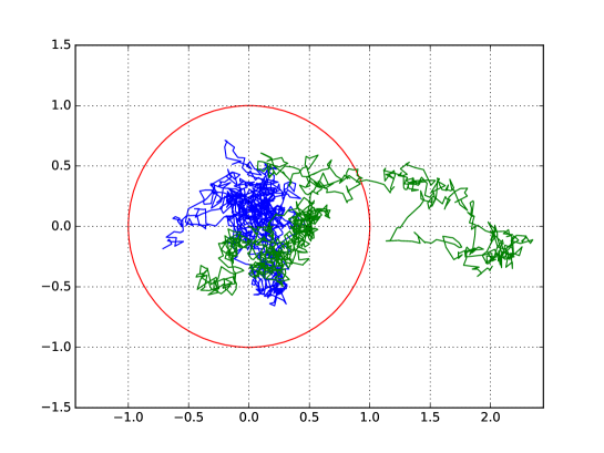
Figure 1: Simulation of a particle trapped by a laser. Within the laser beam (red circle), the particle is subject to two phenomena: (i) a trapping force that pulls the particle towards the center of the beam and (ii) random Brownian perturbations. Outside of the laser beam, the trapping force vanishes very quickly and can be considered as zero [11]. Two sample trajectories for $t\in[0,T]$ are shown in blue and green. The green trajectory leaves the beam at some time $t<T$, after which one has essentially lost all control authority over it. It is therefore crucial, in any probability calculations, to consider the event that the particle is contained within the beam for all $t\in[0,T]$.

Yet, estimating the exit/containment probability is non-trivial: even for linear, uni-dimensional, systems of the following form (also known as Ornstein-Uhlenbeck processes)

$$dX_{t}=-\lambda X_{t}dt+\sigma dB_{t},$$

the containment probability can be computed exactly for only some particular values of $\lambda,\sigma,R,T$ [3]. Kushner’s classic book on stochastic control [6] provides some bounds on the containment probability for nonlinear systems (within the topic of “finite-time stability”) but, as we shall see in Section 2.2, those bounds are too loose for many practical applications.

In this paper, we derive tight bounds on the containment probability for a class of nonlinear stochastic systems. The core idea is to compare the “pull strength” (how hard the deterministic part of the system dynamics pulls towards the origin) experienced by the nonlinear system at hand with that of a well-chosen process for which tight estimates of the containment probability are known or can be numerically obtained (e.g. an Ornstein-Uhlenbeck process). However, a stronger pull everywhere does not always imply a larger containment probability, as made clear in Section 2.3. The main technical contribution of this paper is thus to define a suitable dominance relationship between the pull strengths of two systems and to prove that this dominance relationship implies an order relationship between their containment probabilities.

The remainder of this paper is organized as follows. Section 2 provides the theoretical and practical contexts of the problem at hand. Section 3 presents the main comparison results in dimensions $d=1$ and $d\geq 2$. Section 4 examines these results in the context of contraction theory [8]. Finally, Section 5 concludes by sketching future research directions.

2 Theoretical and practical contexts

2.1 Containment probability vs mean-square stability

The stability of nonlinear stochastic systems is an active research area with important applications ranging from observer and controller design for nonlinear noisy systems [4], to synchronization in networks of noisy oscillators [9, 10], etc.

Most of the existing stochastic stability results are in the “mean-square” sense, typically of the form [9, 4]

$$\forall t\geq 0,\ \operatorname{\mathbf{E}}(\|X_{t}\|^{2})\leq C_{1}+C_{2}e^{-2\lambda t},$$ (1)

where $C_{1},C_{2}$ are two positive constants. While such results are certainly useful to understand the system behavior on average, they are not relevant when it comes to behaviors that depend on individual system trajectories. Consider for instance a microscopic particle that is trapped by a laser tweezer [1] and subject to Brownian perturbations [11]. The motion of the particle is well described by a Stochastic Differential Equation (SDE), but the validity of that description breaks down when the particle escapes from the laser trapping region, see Fig. 1. Mean-square stability results that do not account for this phenomenon will not provide an accurate understanding of the system.

Note that it is possible to use concentration inequalities to derive, from mean-square bounds (1), probabilities of the form

$$\mathbf{P}\left(\|X_{t}\|^{2}\geq(C_{1}+C_{2}e^{-2\lambda t})\beta(\delta)\right)\leq e^{-\delta},$$

see e.g. [4]. However, to be relevant, such probabilities, as the mean-square bounds mentioned previously, must be conditioned upon the containment event.

It is therefore crucial to consider the containment probability of the form

$$\mathbf{P}(\sup_{t\leq T}\|X_{t}\|^{2}\leq R^{2})\geq 1-\varepsilon,$$

where $R$ is the laser trapping radius and $\varepsilon$ a small constant. One can then reason on the particle behavior conditioned upon the above probability that the particle remains confined within the trapping region at all time until time $T$.

Another important example concerns the analysis of the Extended Kalman Filter (EKF) [4]. The SDE describing the EKF is obtained by linearizing the system dynamics around a reference trajectory, and is therefore guaranteed to be valid only within some radius $R$ around that trajectory. One thus needs to condition upon the probability that the system trajectory remains within a radius $R$ from the reference trajectory up to some time horizon $T$. The reader is referred to Chapter III of [6] for an extensive discussion of the relative merits of mean-square stability versus exit/containment probabilities in control theory.

2.2 Looseness of existing containment probability estimates

In the literature, the main result on exit probability for nonlinear systems was derived in Chapter III of Kushner’s book [6], based on a stochastic Lyapunov analysis. However, the bound provided is too loose to be useful in many practical applications. Consider again the laser trapping application [11]. The estimates of the containment probability can be used to calculate the maximum velocity of the laser beam such that the particle remains trapped with high probability. In [11], it was shown that using Kushner’s estimates yields recommended maximum beam velocities that are significantly lower than velocities experimentally found to be safe.

To get a more precise idea, consider the following simple linear, uni-dimensional, stochastic system (an Ornstein-Uhlenbeck process)

$$dX_{t}=-X_{t}dt+\sqrt{2}dB_{t},\ X_{0}=0.$$ (2)

The bound given by Kushner [6] would read

$$\mathbf{P}(\sup_{t\leq T}|X_{t}|\leq R)\geq e^{-\mu_{K}(R)T},\ \textrm{where}$$ (3)

$$\mu_{K}(R)=\frac{2}{R^{2}}.$$ (4)

On the other hand, a direct, but more technically challenging, analysis of system (2), gives the following bound (see [3])

$$\mathbf{P}(\sup_{t\leq T}|X_{t}|\leq R)\sim_{T\to\infty}e^{-\mu_{D}(R)T},$$ (5)

where $\mu_{D}(R)$ is the smallest value $\nu$ such that the Sturm-Liouville system

$$\begin{cases}y^{\prime\prime}(x)-xy^{\prime}(x)=-\nu y(x)\\ y(-R)=y(R)=0\end{cases}$$

has non-null solutions. Reference [3] then gives some values of $\mu_{D}(R)$ for $0.7\leq R\leq 3$, as well as the asymptotics

$$\mu_{D}(R)\sim_{R\to\infty}\frac{R}{\sqrt{2\pi}}e^{-\frac{R^{2}}{2}}.$$ (6)

Note that the asymptotics of (5) and (6) yield very good approximations as soon as $T\geq 5$ and $R\geq 3$.

Fig. 2 compares the decay rate $\mu_{K}$ given by Kushner and the decay rate $\mu_{D}$ obtained by direct analysis. One can observe that $\mu_{K}$ is tight for $R\leq 2$, but becomes very loose for large values of $R$.

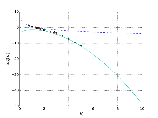
Figure 2: Comparison (in log scale) of the decay rate $\mu_{K}$ given by Kushner (dashed blue) and the decay rate $\mu_{D}$ obtained by direct analysis of the Ornstein-Uhlenbeck process [red stars: exact values; green circles: values obtained by Monte Carlo simulations with $T=5$, cyan plain line: asymptotics for large $R$ given by (6)]. Note that the asymptotics yield very good approximations as soon as $R\geq 3$.

In [11], it was shown, in a physical laser trapping experiment, that, in contrast with Kushner’s estimates (3), the direct estimates (5) yields recommended maximum beam velocities that agree extremely well with the velocities experimentally found to be safe.

2.3 A stronger pull does not always imply a larger containment probability

Consider two uni-dimensional systems (one can get rid of $\sigma$ by adequate normalization)

$$dX_{t} = f(X_{t})dt+dB_{t},$$

$$dY_{t} = g(Y_{t})dt+dB^{\prime}_{t}.$$

Suppose that, everywhere, $X_{t}$ experiences a stronger pull than $Y_{t}$ towards zero, that is,

$$\forall x\in\mathbb{R},\ \mathrm{sgn}(x)f(x)\leq\mathrm{sgn}(x)g(x),$$ (7)

where the sign function defined by

$$\mathrm{if}\ x>0, \mathrm{sgn}(x):=1,$$

$$\mathrm{if}\ x=0, \mathrm{sgn}(x):=0,$$

$$\mathrm{if}\ x<0, \mathrm{sgn}(x):=-1.$$

Then, one would like to say that, for all $T,R$,

$$\mathbf{P}(\sup_{t\leq T}|X_{t}|\leq R)\geq\mathbf{P}(\sup_{t\leq T}|Y_{t}|\leq R).$$ (8)

However, this is not always true, as shown by the following counter-example.

For a given $\lambda\in\mathbb{R}$, denote by $X^{\lambda}$ the strong solution of the SDE

$$dX_{t}=-X_{t}\mathbf{1}_{\left\{X_{t}>0\right\}}dt-\lambda X_{t}\mathbf{1}_{\left\{X_{t}<0\right\}}+dB_{t},$$

i.e. $X^{\lambda}$ is similar to an Ornstein-Uhlenbeck process with pull 1 on the right half-line, and with pull strength $\lambda$ on the left half-line. Note that, if $\lambda>\lambda^{\prime}$, then $X^{\lambda}$ is subject to a pull stronger or equal to that of $X^{\lambda^{\prime}}$ everywhere.

Given $R,T$, consider the containment probability

$$P(\lambda):=\mathbf{P}\left(\sup_{t\leq T}|X^{\lambda}_{t}|\leq R\right).$$

Fig. 3 shows the values of $P(\lambda)$ for $\lambda\geq 1$, $R=0.5$, $T=1$. One can observe that $P(\lambda)$ is non-monotonic: it increases on the right of $\lambda=1$, reaches a maximum at $\lambda\simeq 20$, then decreases towards $P(1)$ when $\lambda\to\infty$.

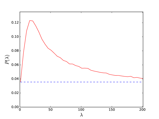
Figure 3: A stronger pull does not always imply a larger containment probability. The red plain line shows the containment probability $P(\lambda)$ for $\lambda\geq 1$ with $R=0.5,T=1$ (obtained by Monte Carlo simulation). One can note that the containment probability increases with the pull strength $\lambda$ only until $\lambda\simeq 20$, then it decreases towards $P(1)$ when $\lambda\to\infty$ (dashed blue line).

Intuitively, increasing the strength of the pull on the left half-line has two opposite effects:

1. A stronger pull on the left half-line makes exits by the left boundary more “difficult”, thereby contributing positively to the containment probability;

2. But, at the same time, increasing the pull strength asymmetrically might “chase” the diffusion from an area where it is well-controlled towards an area where the control is not as good, which can, in turn, help the process escape. In the limit $\lambda\to\infty$, the left half-line acts as a solid wall. Therefore, $\lim_{\lambda\to\infty}X^{\lambda}=|X^{1}|$, which implies that $\lim_{\lambda\to\infty}P(\lambda)=P(1)$.

For small values of $\lambda$, the first effect dominates, while for large values of $\lambda$, the second effect does, as can be observed in Fig. 3. Thus, for $\lambda$ large enough, the containment probability decreases with $\lambda$, which contradicts the intuition of (8).

In the next section, we shall define a suitable dominance relationship between the pull strengths, that is, one that implies an order relationship between the containment probabilities.

3 Comparison Theorem under symmetric dominance assumption

3.1 Comparison Theorem in dimension $d=1$

To avoid the phenomenon of concentration in “safe havens” where exits are subsequently easier, one can “symmetrize” the dominance assumption of (7) as in the following Theorem (see Fig. 4 for illustration).

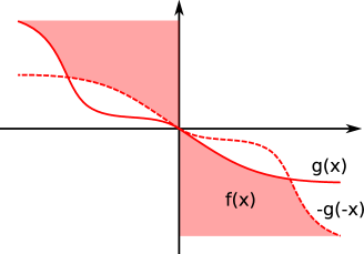
Figure 4: Symmetrization of the dominance assumption.

Theorem 1 (Comparison Theorem in dimension 1).

Let $f,g$ be continuous functions satisfying

$$\forall x\in[0,K], f(x)\leq\min(g(x),-g(-x))$$

$$\forall x\in[-K,0], f(x)\geq\max(g(x),-g(-x)),$$ (9)

then, given the SDEs

$$dX_{t} = f(X_{t})dt+\mathrm{sgn}(X_{t})dB_{t}$$

$$dY_{t} = g(Y_{t})dt+\mathrm{sgn}(Y_{t})dB_{t},$$

one has almost surely $|X_{t}|\leq|Y_{t}|$ for all $t\leq T_{K}:=\inf\{t>0:|Y_{t}|=K\}$. In particular, one has

$$\forall R\in(0,K],\ \forall T\geq 0,\ \mathbf{P}(\sup_{t\leq T}|X_{t}|\leq R)\geq\mathbf{P}(\sup_{t\leq T}|Y_{t}|\leq R).$$

Note that the processes $X$ and $Y$ and defined using the same noise process $B$ – a technique called coupling [7]. Heuristically, the coupling is as follows

• if $X_{t}$ and $Y_{t}$ have the same sign, then $X_{t+dt}$ and $Y_{t+dt}$ are constructed using the same noise;

• if $X_{t}$ and $Y_{t}$ have opposite sign, then $X_{t+dt}$ and $Y_{t+dt}$ are constructed using opposite noises.

Thus, in both cases, the absolute values of $X_{t}$ and $Y_{t}$ move in the same direction.

The main difficulty in proving Theorem 1 is the time instants when $X$ and $Y$ go close to 0. We shall tackle this difficulty by an approximation technique. Consider the stronger assumptions of the following Lemma.

Lemma 1.

Let $f,g$ be continuous functions satisfying (1). Assume moreover that there exists $\varepsilon>0$ such that

$$\forall|x|\leq\varepsilon,\ f(x)=g(x).$$ (10)

Then the conclusions of Theorem 1 hold.

Proof.

Note first that (10) and (1) together imply that

$$\forall|x|\leq\varepsilon,\ -f(-x)=f(x)=g(x)=-g(-x).$$

Let $B$ be a standard Brownian motion, we construct on the same probability space two processes $X$ and $Y$ satisfying

$$X_{0} = Y_{0}=0$$

$$X_{t} = \int_{0}^{t}f(X_{s})ds+\int_{0}^{t}\mathrm{sgn}(X_{s})dB_{s}$$ (11)

$$Y_{t} = \int_{0}^{t}g(Y_{s})ds+\int_{0}^{t}\mathrm{sgn}(Y_{s})dB_{s}.$$ (12)

Note that there is no trajectorial uniqueness for this type of stochastic differential equation. However, there exist solutions, and uniqueness in law holds by boundedness of $f$ and $g$ on compact intervals.

Given a solution $Y$ of (12), define a sequence of hitting times as follows. Let $\tau^{(0)}:=0$ and

$$\upsilon^{(k)}:=\inf\{t>\tau^{(k)}:|Y_{t}|=\varepsilon\};\quad\tau^{(k+1)}:=\inf\{t>\upsilon^{(k)}:Y_{t}=0\}.$$

In other words, $\upsilon^{(k)}$ is the first time, after time $\tau^{(k)}$, that $Y$ leaves the strip $[-\varepsilon,\varepsilon]$, and $\tau^{(k+1)}$ is the first time, after time $\upsilon^{(k)}$, that $Y$ hits $0$.

We now construct $X$ as follows (see Fig. 5 for sample paths of $X$ and $Y$)

• For all $t\in[\tau^{(k)},\upsilon^{(k)}]$, $X_{t}=Y_{t}$;

• On $[\upsilon^{(k)},\tau^{(k+1)}]$, $X$ is the unique solution of (11) on this interval.

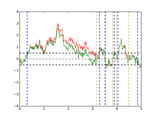
Figure 5: Sample trajectories for the processes $X$ (green) and $Y$ (red). Here $\varepsilon=0.5$ (black dashed lines). The hitting times $\tau$ (dashed yellow) and $\upsilon$ (dashed blue) are also indicated. Note that $X=Y$ in the intervals [yellow, blue] and $|X|\leq|Y|$ in the intervals [blue, yellow].

We show, by induction on $k\in\mathbb{N}$, the following properties of $X$

(i)

$X$ is a solution of (11) on $[\tau^{(k)},\upsilon^{(k)}]$ and $[\upsilon^{(k)},\tau^{(k+1)}]$;

(ii)

$|X|\leq|Y|$ in the above intervals;

(iii)

$X_{\tau^{(k+1)}}=0$.

Initialization: (i) For $k=0$, note that, for all $t\in[\tau^{(0)},\upsilon^{(0)}]$, $X_{t}=Y_{t}\leq\varepsilon$. Thus, by (10), one has $f(X_{t})=g(Y_{t})$ over the whole interval, which in turn implies that $X=Y$ is a solution of (11) on the interval. The fact that $X$ is a solution of (11) on $[\upsilon^{(0)},\tau^{(1)}]$ is by construction.

(ii) Next, $|X_{t}|\leq|Y_{t}|$ trivially on $[\tau^{(0)},\upsilon^{(0)}]$. On $[\upsilon^{(0)},\tau^{(1)}]$, one has, by Itô-Tanaka formula

$$|X_{t}| = \int_{0}^{t}\mathrm{sgn}(X_{s})f(X_{s})ds+B_{t}+L^{X}_{t}$$

$$|Y_{t}| = \int_{0}^{t}\mathrm{sgn}(Y_{s})g(Y_{s})ds+B_{t}+L^{Y}_{t},$$

where $L^{X}$ and $L^{Y}$ are the local times at $0$ of $X$ and $Y$ respectively. This yields

$$|Y_{t}|-|X_{t}|=\int_{0}^{t}\mathrm{sgn}(Y_{s})g(Y_{s})-\mathrm{sgn}(X_{s})f(X_{s})ds+L^{Y}_{t}-L^{X}_{t}.$$ (13)

Assume by contradiction that there exists some time $t\in[\upsilon^{(0)},\tau^{(1)})$ such that $|X_{t}|=|Y_{t}|$, and $|X_{t+u}|>|Y_{t+u}|>0$ for all $u>0$ small enough. As both $|X_{t+u}|$ and $|Y_{t+u}|$ are different from $0$ for $u$ close enough to $0$, one has that $L^{X}$ and $L^{Y}$ are constant in a neighbourhood of $t$. Therefore, by (13), $h:t\mapsto|Y_{t}|-|X_{t}|$ is differentiable in a neighborhood of $t$, and its derivative is, in that neighborhood,

$$h^{\prime}(s)=\mathrm{sgn}(Y_{s})g(Y_{s})-\mathrm{sgn}(X_{s})f(X_{s})\geq 0,$$

which contradicts the fact that $|X_{t+u}|>|Y_{t+u}|$ for $u$ small enough.

We have thus shown that $|X_{t}|\leq|Y_{t}|$ on $[\upsilon^{(0)},\tau^{(1)})$. The inequality can be extended to the closed interval by continuity.

(iii) Since $|X|\leq|Y|$ on the interval $[\upsilon^{(0)},\tau^{(1)}]$ and that $Y_{\tau^{(1)}}=0$, one has $X_{\tau^{(1)}}=0$.

Induction: By the induction hypothesis, one has $X_{\tau^{(k)}}=Y_{\tau^{(k)}}=0$. Thus the proof that $|X_{s}|\leq|Y_{s}|$ for $s\in[\tau^{(k)},\tau^{(k+1)}]$ is straightforward by using the Markov property and adapting the Initialization step.

To complete the proof, note that $\lim_{k\to\infty}\tau^{(k)}=\infty$, which can be obtained by observing that, by the law of large numbers, one has almost surely

$$\lim_{k\to\infty}\frac{1}{k}\sum_{j=1}^{k}\upsilon^{(j)}-\tau^{(j)}=\operatorname{\mathbf{E}}(\upsilon^{(1)})>0.$$

∎

We are now in a position to prove Theorem 1.

Proof.

Let $f$ and $g$ be two functions satisfying (1). For all $\varepsilon>0$, we set

$$f^{\varepsilon}(x) := \mathbf{1}_{\left\{x>2\varepsilon\right\}}f(x-2\varepsilon)+\mathbf{1}_{\left\{x<-2\varepsilon\right\}}f(x+2\varepsilon)$$

$$g^{\varepsilon}(x) := \mathbf{1}_{\left\{x>\varepsilon\right\}}g(x-\varepsilon)+\mathbf{1}_{\left\{x<-\varepsilon\right\}}g(x+\varepsilon).$$

Note that $f^{\varepsilon},g^{\varepsilon}$ satisfy (1) and (10), therefore, by Lemma 1, the conclusions of Theorem 1 hold for $X^{\varepsilon}$ and $Y^{\varepsilon}$. Next, since the law of $(X^{\varepsilon},Y^{\varepsilon})$ converges toward the law of $(X,Y)$, one can conclude, by Skorokhod’s embedding theorem, that there is trajectorial convergence, and that the limiting process $(X,Y)$ satisfies the conclusion of Theorem 1. ∎

Remark 1.

If $Y$ is an Ornstein-Uhlenbeck process with pull strength $\lambda$, then condition (1) becomes

$$\forall x\in[-K,K],\ \mathrm{sgn}(x)f(x)\leq-\lambda|x|.$$

3.2 Comparison Theorem in dimension $d\geq 2$

To enforce a “symmetric” dominance assumption in dimension $d\geq 2$, we introduce the radial decomposition: for $x\in\mathbb{R}^{d}\backslash\{0\}$, denote by $R_{x}$ the matrix of the rotation that brings $\frac{x}{\|x\|}$ to the first basis vector $e_{1}$ (by convention, $R_{0}:=\mathrm{Id}$). Theorem 1 can now be extended to dimension $d\geq 2$ as follows.

Theorem 2 (Comparison Theorem in dimension $d\geq 2$).

Let $f,g$ be continuous functions satisfying

$$\forall r\in\mathbb{R}_{+},\ \sup_{\theta\in\mathbb{S}_{d-1}}f(r\theta)^{\top}\theta\leq\inf_{\theta\in\mathbb{S}_{d-1}}g(r\theta)^{\top}\theta.$$ (14)

then, given the SDEs

$$dX_{t} = f(X_{t})dt+R_{X_{t}}^{-1}dB_{t}$$

$$dY_{t} = g(Y_{t})dt+R_{Y_{t}}^{-1}dB_{t},$$

one has almost surely $\|X_{t}\|\leq\|Y_{t}\|$ for all $t\leq T_{K}:=\inf\{t>0:\|Y_{t}\|=K\}$. In particular, one has

$$\forall R\in(0,K],\ \forall T\geq 0,\ \mathbf{P}(\sup_{t\leq T}\|X_{t}\|\leq R)\geq\mathbf{P}(\sup_{t\leq T}\|Y_{t}\|\leq R).$$

Proof.

We follow the same strategy as in the proof of Theorem 2. Note that, using Itô-Tanaka formula in dimension $d\geq 2$, one has

$$||X_{t}||=\int_{0}^{t}f(X_{s})^{\top}\frac{X_{s}}{||X_{s}||}ds+B_{t}.e_{1}+L^{X}_{t},$$

and a similar formula for $Y$, where

$$L^{X}_{t}:=\lim_{\varepsilon\to 0}\frac{1}{V_{d}\varepsilon^{d}}\int_{0}^{t}\mathbf{1}_{\left\{||X_{s}||\leq\varepsilon\right\}}ds.$$

The rest of the proof is similar to that of Theorem 2. ∎

Remark 2.

If $Y$ is an Ornstein-Uhlenbeck process with pull strength $\lambda$, then condition (14) becomes

$$\forall r\in\mathbb{R}_{+},\ \sup_{\theta\in\mathbb{S}_{d-1}}f(r\theta)^{\top}\theta\leq-\lambda r.$$

4 Link with contraction theory

Contraction theory [8] provides a set of tools to analyze the exponential stability of nonlinear systems, and has been applied notably to observer design (see e.g. [2]), synchronization analysis (see e.g. [10]), and systems neuroscience. Nonlinear contracting systems enjoy desirable aggregation properties, in that contraction is preserved under many types of system combinations given suitable simple conditions [8].

We say that $f$ is contracting with contraction rate $\lambda>0$ in the identity metric [8] if

$$\forall x,t,\ \lambda_{\max}\left(\frac{\partial f}{\partial x}\right)\leq-\lambda,$$

where $\lambda_{\max}(A)$ denotes the largest eigenvalue of the symmetric part of matrix $A$. A specialized result of contraction theory is that, if $f$ is contracting with contraction rate $\lambda$, then all system trajectories converge exponentially to a single trajectory, with convergence rate $\lambda$. More general settings of contraction theory can cater for the dependency of $f$ on the time parameter $t$ as well as nonlinear metrics. For simplicity, however, our current discussion is carried out without the dependency of $f$ on $t$ and in the identity metric. Including time-dependency could be addressed by adapting condition (14) to include uniformity over $t\in\mathbb{R}$ and $\omega\in\Omega$. Extension to nonlinear metrics would likely involve checking whether the metrics are compatible with the symmetric dominance assumption. Such extensions will be investigated in our future work.

Assume now that $f$ is contracting with contraction rate $\lambda$ in the identity metric and consider two $d$-dimensional SDEs

$$dX_{t} = f(X_{t})dt+\sigma dB^{X}_{t}$$

$$dY_{t} = f(Y_{t})dt+\sigma dB^{Y}_{t}.$$

Consider the $d$-dimensional process $Z:=Y-X$. One has

$$dZ_{t}=dY_{t}-dX_{t}=[f(Y_{t})-f(X_{t})]dt+\sqrt{2}\sigma dB^{Z}_{t}.$$

Since $f$ is smooth, one can write 

$$f(Y_{t})-f(X_{t}) = \left(\int_{0}^{1}\frac{\partial f}{\partial x}(X_{t}+s(Y_{t}-X_{t}))ds\right)(Y_{t}-X_{t})$$

$$=: g(X_{t},Y_{t})Z_{t}.$$

Thus, one can rewrite

$$dZ_{t}=g(X_{t},Y_{t})Z_{t}dt+\sqrt{2}\sigma dB^{Z}_{t},$$

where $g(X_{t},Y_{t})$ can be seen as an external driving signal.

Define $h(z):=g(x,y)z$. Let us evaluate the radial component of $h$. For that, set $z=r\theta$ where $r>0$, $\theta\in\mathbb{S}_{d-1}$. One has

$$h(r\theta)^{\top}\theta = \frac{1}{r}(g(x,y)z)^{\top}z$$

$$= \frac{1}{r}z^{\top}\left(\int_{0}^{1}\frac{\partial f}{\partial x}(x+s(y-x))ds\right)^{\top}z$$

$$= \frac{1}{r}\int_{0}^{1}z^{\top}\left(\frac{\partial f}{\partial x}(x+s(y-x))\right)^{\top}zds$$

$$\leq \frac{1}{r}\int_{0}^{1}-\lambda\|z\|^{2}ds=-\lambda r.$$

Since $-\lambda r$ is the radial component of a $d$-dimensional Ornstein-Uhlenbeck process with pull strength $\lambda$ (see Remark 2), Theorem 2 can be used to bound the containment probabilities for the distance $\mathbf{P}(\sup_{t\leq T}\|Y_{t}-X_{t}\|\leq R)$ by the corresponding containment probabilities of a $d$-dimensional Ornstein-Uhlenbeck process with pull strength $\lambda$ and noise strength $\sqrt{2}\sigma$.

5 Conclusion

We have defined a dominance relationship between the pull strengths of two nonlinear stochastic systems that implies an order relationship between their containment probabilities. This result enables establishing tight bounds on the containment probabilities for a large class of nonlinear systems by comparing them with suitable Ornstein-Uhlenbeck processes, for which containment probabilities can be numerically obtained.

One important implication of this result is that one can immediately bound the containment probabilities of stochastic systems that are contracting with rate $\lambda$ by those of Ornstein-Uhlenbeck processes with pull strength $\lambda$.

The results presented here may have many exciting applications in control theory. For example, the design of controllers for optical manipulation in [11] could be extended to deal with nonlinear trapping forces. Another application could be to develop a rigorous theory of stability for Extended Kalman Filters, e.g. by extending the contraction-theory-based analysis of [2] to stochastic systems. Yet another avenue would be to establish tight bounds on the time taken by stochastic optimization algorithms – such as the Stochastic Gradient Descent widely used in machine learning – to escape local minima [5]. Exploring such applications is the subject of ongoing research.

References

- [1] A. Ashkin, J. M. Dziedzic, J. Bjorkholm, and S. Chu. Observation of a single-beam gradient force optical trap for dielectric particles. Optics letters, 11(5):288–290, 1986.
- [2] S. Bonnabel and J.-J. Slotine. A contraction theory-based analysis of the stability of the deterministic extended kalman filter. IEEE Transactions on Automatic Control, 60(2):565–569, 2014.
- [3] S. Finch. Ornstein-uhlenbeck process. http://citeseerx.ist.psu.edu/viewdoc/summary?doi=10.1.1.710.4200, 2004. Accessed: 2018-10-05.
- [4] T. Karvonen, S. Bonnabel, E. Moulines, and S. Särkkä. On stability of a class of filters for non-linear stochastic systems. arXiv preprint arXiv:1809.05667, 2018.
- [5] R. Kleinberg, Y. Li, and Y. Yuan. An alternative view: When does sgd escape local minima? arXiv preprint arXiv:1802.06175, 2018.
- [6] H. Kushner. Stochastic Stability and Control. Academic Press, 1967.
- [7] T. Lindvall. Lectures on the coupling method. Courier Corporation, 2002.
- [8] W. Lohmiller and J.-J. E. Slotine. On contraction analysis for non-linear systems. Automatica, 34(6):683–696, 1998.
- [9] Q.-C. Pham, N. Tabareau, and J.-J. Slotine. A contraction theory approach to stochastic incremental stability. IEEE Transactions on Automatic Control, 54(4):816–820, 2009.
- [10] N. Tabareau, J.-J. Slotine, and Q.-C. Pham. How synchronization protects from noise. PLoS computational biology, 6(1):e1000637, 2010.
- [11] X. Yan, C. C. Cheah, Q. M. Ta, and Q.-C. Pham. Stochastic dynamic trapping in robotic manipulation of micro-objects using optical tweezers. IEEE Transactions on Robotics, 32(3):499–512, 2016.