Variation of shear moduli across superconducting phase transitions

Abstract

We study how shear moduli of a correlated metal change across superconducting phase transitions. Using a microscopic theory we explain why for most classes of superconductors this change is small. The Fe-based and the A15 systems are notable exceptions where the change is boosted by five orders of magnitude. We show that this boost is a consequence of enhanced nematic correlation. The theory explains the unusual temperature dependence of the orthorhombic shear and the back-bending of the nematic transition line in the superconducting phase of the Fe-based systems.

An important topic in the field of high temperature superconductivity is to understand the interplay between superconducting and nematic orders. The issue arises naturally for the Fe-based systems whose phase diagram shows a ubiquitous presence of the two orders review-feas ; kuo-fisher-2016 ; chowdhury-2011 ; Livanas ; fernandes-2013 ; glasbrenner-2015 ; mishra-2016 ; gallais-2016 ; sprau-2017 ; andersen-2017 ; classen-2017 ; benfatto-2018 . The relevance of nematicity to understand the pseudogap state of the cuprate superconductors is currently under active investigation as well ando-2002 ; howald-2003 ; hinkov-2008 ; daou-2010 ; sato-2017 ; auvray-gallais-2019 ; kivelson-2003 ; vojta-2009 ; wang-2013 .

One cause of interplay is fluctuations associated with the two orders, and the effect of nematic fluctuations on superconductivity has been extensively studied in the past yamase-2013 ; maier-2014 ; metlitski-2015 ; lederer-2015 ; labat-2017 ; klein-2018 ; lederer-2019 . A second cause can be a third degree of freedom such as antiferromagnetic fluctuations which can enhance nematic correlation, but which are themselves suppressed in a singlet superconductor fernandes-2010 . What is less examined is the effect of the superconducting order itself on the nematic properties of electrons in solids. The goal of the current paper is to study the last from a microscopic point of view.

For such a study a shear strain of a suitable symmetry is an appropriate nematic order parameter, even if the nematic transition is driven by electronic interactions fernandes-2014 ; gallais-review-2016 . This is because, due to electron-strain coupling, the nematic transition at temperature $T_{s}$ itself manifests as a structural instability. Consequently, tracking the shear elastic constant $c_{s}(T)$ as a function of temperature $T$, especially across the superconducting transition at $T_{c}$, is a practical method to study the interplay. For simplicity we restrict to the case where $T_{c}>T_{s}$.

More concretely, for $T\sim T_{c}$, the free energy per unit volume involving the shear strain $u_{s}$ and the superconducting order parameter $\Delta$ can be written as

$$F=(c_{s}/2)u_{s}^{2}+(a/2)\left|\Delta\right|^{2}+(b/4)\left|\Delta\right|^{4}+(\lambda/2)u_{s}^{2}\left|\Delta\right|^{2}.$$ (1)

Here $\Delta$ has dimension of energy, while $(a,\lambda)$ have that of density of states (DOS), $a=a_{0}(T-T_{c})$, and $b>0$. The fourth term, which captures the interplay, describes how the shear elastic constant is modified across $T_{c}$. In the above we assumed that $\Delta$ belongs to a one dimensional irreducible representation of the unit cell point group, and that there is no second nearly critical symmetry channel for superconductivity Livanas ; fernandes-2013 ; kushnirenko-2018 .

From Eq. (1) it follows that $c_{s}(T)$ itself is continuous at $T_{c}$, but its temperature derivative jumps at $T_{c}$ with the jump given by $(dc_{s}/dT)_{T_{c}^{+}}-(dc_{s}/dT)_{T_{c}^{-}}=\lambda a_{0}/b$. In other words, $c_{s}(T)$ has a kink at $T_{c}$ which encodes information about the interplay parameter $\lambda$. The magnitude of this kink can be quantified by $\delta c_{s}/|c_{s}^{m}|$, where $\delta c_{s}\equiv\lambda\Delta_{0}^{2}\sim c_{s}^{s}-c_{s}^{m}$. Here $c_{s}^{s}$ is the zero temperature elastic constant in the superconducting phase, $c_{s}^{m}$ is inferred from the $T=0$ extrapolation of $c_{s}(T)$ in the metal phase, and $\Delta_{0}\equiv\Delta(T=0)$.

A literature search reveals that in most known classes of superconductors the ratio $\delta c_{s}/|c_{s}^{m}|$ is “small” and is of order $10^{-6}$. Examples include conventional Bardeen-Cooper-Schrieffer (BCS) systems olsen ; alers61 , cuprates such as La_2-xSr_xCuO₄ at various dopings (see Figs. 7 and 8 in Ref. nohara ), and heavy fermion systems UPt₃ and URu₂Si₂ bruls ; thalmeier . From Ehrenfest-type thermodynamic argument it is known that $\delta c_{s}/|c_{s}^{m}|$ is related to the ratio between the superconducting condensation energy and the Fermi energy, which is typically small testardi75 ; millis-rabe . This provides a simple way to understand this small ratio without a microscopic analysis.

However, there are two classes of superconductors, namely the Fe-based fernandes-2010 ; yoshizawa ; zvyagina13 ; boehmer-2014 ; boehmer-2016 and the A15 systems testardi-67 ; rehwald-72 ; testardi-rmp , for which this ratio is “large” with $\delta c_{s}/|c_{s}^{m}|\sim 10^{-1}$. Clearly, this increase of $\delta c_{s}/|c_{s}^{m}|$ by five orders of magnitude compared to the standard behavior cannot be understood purely from thermodynamics, and a microscopic approach is needed. With this motivation, here we develop such a microscopic theory of the coupling $\lambda$ that encodes the interplay between the two orders.

Our main results are the following. (i) First, we show that in systems with negligible nematic correlation $\lambda/\mathcal{N}_{F}$ is small, where $\mathcal{N}_{F}$ is DOS at Fermi level. This is due to a cancellation of the low-energy electronic contribution that is not imposed by symmetry. We show that this cancellation is related to the general property that the quadrupolar charge susceptibility of an electronic system remains approximately unchanged between its metallic and superconducting phases. This explains the small ratio of $\delta c_{s}/|c_{s}^{m}|$ for most superconductors. (ii) Second, we show that for systems with large nematic correlation length $\xi\gg l$, where $l$ is the interatomic distance, the parameter $\lambda$ is boosted by $(\xi/l)^{4}$. This accounts for the five orders of magnitude increase in $\delta c_{s}/|c_{s}^{m}|$ seen in the A15 and the Fe-based systems. (iii) Third, we show that the sign of $\lambda$, that controls cooperation or competition between the two orders, is non-universal and that it depends on the band structure.

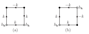
Figure 1: Diagrammatic representation of the coupling $\lambda$ that controls the interplay between superconducting and nematic orders, see Eq. (1). $\lambda$ is a four-point function with two particle-hole (open circles) vertices with nematic form factor $h_{\bf k}$ and two particle-particle (closed circles) vertices, see Eq. (Variation of shear moduli across superconducting phase transitions). Solid lines are electron Green’s functions. $k=({\bf k},\omega)$ denote momentum and frequency.

Microscopic theory. Our main message can be illustrated by considering a one-band metal in a tetragonal lattice. The relevant elastic constant can be written as

$$c_{s}(T)\equiv c_{0}-\alpha^{2}\chi_{n}(T).$$ (2)

$c_{0}$ is the modulus of the bare elastic medium, which we assume to be temperature independent. $\alpha$ is the electron-strain interaction energy, such that in the presence of a finite strain the electron dispersion changes as $\epsilon_{{\bf k}}\rightarrow\tilde{\epsilon}_{{\bf k}}=\epsilon_{{\bf k}}+\alpha u_{s}h_{{\bf k}}$. To be concrete we take $u_{s}$ to be the orthorhombic strain that transform as $(x^{2}-y^{2})$, in which case $h_{{\bf k}}\sim\cos k_{x}-\cos k_{y}$. The precise nature of the shear mode and the associated form factor is unimportant. Likewise, the spatial symmetry of $\Delta$ (i.e., $s$-, $p$- or $d$-wave) play no role, and we take it as $s$-wave for simplicity. The quantity $\chi_{n}\equiv\lim_{{\bf q}\rightarrow 0}\chi_{n}({\bf q},\omega=0)$, where $\chi_{n}({\bf q},0)$ is the static nematic susceptibility of the electrons. Thus, the role of the lattice variables is simply to probe the electronic properties, in particular how $\chi_{n}$ changes across $T_{c}$.

At this point it is convenient to distinguish the following two situations.

(a) Away from nematic instability. When the system is far away from nematic/orthorhombic instability the nematic correlation length is negligible, and therefore $\chi_{n}^{s/m}({\bf q},0)\approx\Pi_{n}^{s/m}({\bf q},0)$, where $\Pi_{n}^{s/m}({\bf q},0)$ is the bare nematic susceptibility. We added superscripts $(s,m)$ to denote superconducting and metallic phases, respectively. In the superconducting phase the bare nematic susceptibility is

$$\Pi_{n}^{s}({\bf q},0) =-\frac{2}{\beta V}\sum_{\omega_{n},{\bf k}}f^{2}_{{\bf k},{\bf q}}[G_{{\bf k}+{\bf q}}(i\omega_{n})G_{{\bf k}}(i\omega_{n})$$

$$-F_{{\bf k}+{\bf q}}(i\omega_{n})F_{{\bf k}}(i\omega_{n})],$$

where $\beta$ is inverse temperature, $V$ is volume, $f_{{\bf k},{\bf q}}\equiv(h_{{\bf k}}+h_{{\bf k}+{\bf q}})/2$ is the nematic form factor, $G_{{\bf k}}(i\omega_{n})=-(i\omega_{n}+\epsilon_{{\bf k}})/(\omega_{n}^{2}+E_{{\bf k}}^{2})$, $F_{{\bf k}}(i\omega_{n})=\Delta/(\omega_{n}^{2}+E_{{\bf k}}^{2})$, and $E_{{\bf k}}=\sqrt{\epsilon_{{\bf k}}^{2}+\Delta^{2}}$. An overall factor two is due to spins. The equivalent expression for $\Pi_{n}^{m}({\bf q},0)$ is obtained by setting $\Delta=0$.

Eqs. (1) and (2) give $\lambda=-(\alpha^{2}/2)[\partial^{2}\chi_{n}^{s}/(\partial|\Delta|^{2})]_{|\Delta|=0}$. Thus, $\lambda$ is a four-point function that can be obtained from $\Pi_{n}^{m}(0,0)$ by inserting two particle-particle vertices (see Fig. 1). This leads to the microscopic expression

$$\lambda=\lambda_{0} \equiv-\frac{2\alpha^{2}}{\beta V}\sum_{\omega_{n},{\bf k}}h^{2}_{{\bf k}}\left[2G^{0}_{{\bf k}}(i\omega_{n})^{3}G^{0}_{{\bf k}}(-i\omega_{n})\right.$$

$$+\left.G^{0}_{{\bf k}}(i\omega_{n})^{2}G^{0}_{{\bf k}}(-i\omega_{n})^{2}\right],$$ (3)

with $G^{0}_{{\bf k}}(i\omega_{n})^{-1}\equiv i\omega_{n}-\epsilon_{{\bf k}}.$ The above frequency sum is simple to perform. We define the $B_{1g}$ density of states as $\mathcal{N}_{B_{1g}}(\epsilon)\equiv(1/V)\sum_{{\bf k}}h^{2}_{{\bf k}}\,\delta(\epsilon-\epsilon_{{\bf k}}),$ and we get

$$\lambda_{0}=-\frac{\alpha^{2}}{2}\int_{-\infty}^{\infty}d\epsilon\mathcal{N}_{B_{1g}}(\epsilon)\frac{d^{2}}{d\epsilon^{2}}\left[\tanh(\beta\epsilon/2)/\epsilon\right].$$

We expand $\mathcal{N}_{B_{1g}}$ around the Fermi energy as $\mathcal{N}_{B_{1g}}(\epsilon)\approx\mathcal{N}_{B_{1g}}(0)+\epsilon\mathcal{N}_{B_{1g}}^{\prime}(0)+(\epsilon^{2}/2)\mathcal{N}_{B_{1g}}^{\prime\prime}(0)+\cdots$, where primes imply derivatives with respect to energy. Remarkably, the term proportional to $\mathcal{N}_{B_{1g}}(0)$, which is the contribution from the low-energy excitations, vanishes. Since the term proportional to $\mathcal{N}_{B_{1g}}^{\prime}(0)$ is trivially zero, the first non-zero contribution is proportional to $\mathcal{N}_{B_{1g}}^{\prime\prime}(0)$. We get,

$$\lambda_{0}=-\alpha^{2}\mathcal{N}_{B_{1g}}^{\prime\prime}(0)\left\{\log[\Lambda/(2T)]+\mathcal{C}_{1}\right\},$$ (4)

where $\mathcal{C}_{1}\equiv\gamma-3/2-\log(\pi/4)$, $\gamma$ is the Euler constant, and $\Lambda$ is a high-temperature cutoff. The logarithmic temperature dependence above has the same origin as the familiar $\log(T)$ dependence of the particle-particle susceptibility in BCS theory.

The cancellation of the low-energy electronic contribution is important, and consequently it is useful to understand better its physical origin. Clearly, the cancellation is not dictated by any symmetry. Instead, it is a consequence of the property that the bare quadrupolar charge susceptibility of electrons remains nearly unchanged across a metal to superconductor transition. This can be demonstrated by the following calculation.

The frequency sum in the expression for $\Pi_{n}^{s}(0,0)$ gives

$$\Pi_{n}^{s}(0,0)=\frac{1}{V}\sum_{{\bf k}}h_{{\bf k}}^{2}\frac{\partial}{\partial\epsilon_{{\bf k}}}\left[\frac{\epsilon_{{\bf k}}}{E_{{\bf k}}}\tanh\frac{E_{{\bf k}}}{2T}\right].$$

If we neglect the energy dependence of the $B_{1g}$ density of states $\mathcal{N}_{B_{1g}}(\epsilon)$, which is appropriate for the low-energy electronic contribution, after the energy integral we get

$$\Pi_{n}^{s}(0,0)_{\rm low}=\Pi_{n}^{m}(0,0)_{\rm low}=2\mathcal{N}_{B_{1g}}(0).$$ (5)

In the above the subscript “low” implies the low-energy contribution. In other words, from the perspective of the low-energy electrons $\Pi_{n}^{s}(0,0)$ is independent of $\Delta$. This property is reminiscent of that of the uniform charge susceptibility $\partial n/\partial\mu$, where $n$ is the electron density and $\mu$ the chemical potential. It is known that the Thomas-Fermi screening length, which is controlled by the uniform charge susceptibility, remains practically unchanged when a metal turns into a superconductor koyama04 . The above discussion implies that if $\Pi_{n}^{s}(0,0)$ is expanded around $\Pi_{n}^{m}(0,0)$ in powers of $|\Delta|^{2}$, order by order the pre-factors would be zero if we neglect the energy dependence of $\mathcal{N}_{B_{1g}}(\epsilon)$. The coupling $\lambda_{0}$ in Eq. (Variation of shear moduli across superconducting phase transitions) is related to the prefactor at order $|\Delta|^{2}$ in this expansion.

The above low-energy cancellation has the following consequences. (i) Most importantly, we conclude that for superconductors with negligible nematic correlation $\delta c_{s}/|c_{s}^{m}|\sim(T_{c}/E_{F})^{2}$, where $E_{F}$ is the Fermi energy. This follows from the estimate $\mathcal{N}_{B_{1g}}^{\prime\prime}(0)\sim\mathcal{N}_{F}/E_{F}^{2}$, and by estimating the electron-phonon interaction energy $\alpha$ as the geometric mean of the typical electronic and elastic energy scales, i.e., $(\alpha^{2}\mathcal{N}_{F}/c_{s})\sim 1$ agd . Thus, the above estimation, backed by a microscopic calculation, explains the order of magnitude of $\delta c_{s}/|c_{s}^{m}|$ reported for most known superconductors, the Fe-based and the A15 systems being exceptions. (ii) The sign of $\lambda_{0}$, which governs whether the two orders cooperate or compete, is non-universal and it depends on the sign of $\mathcal{N}_{B_{1g}}^{\prime\prime}(0)$. (iii) Due to the absence of the low-energy contribution the coupling $\lambda\sim\lambda_{0}$ is nearly temperature independent. This is consistent with the weak $T$-dependence of $\chi_{n}$ of several Fe-based systems at doping well away from the nematic instability reported from elastoresistivity chu2012 and electronic Raman studies gallais2013 ; blumberg2016 .

(b) Near a nematic instability. The above considerations need modification if the system is in the vicinity of a nematic instability, and the nematic correlation length $\xi\gg l$, where $l$ is the interatomic distance. For the sake of simplicity we assume that the nematic instability is a Pomeranchuk transition, i.e., spontaneous deformation of the Fermi surface. Accordingly, we postulate the presence of an interaction $\mathcal{H}_{I}=-(g/2)\sum_{{\bf q}}O_{n}(-{\bf q})O_{n}({\bf q}),$ with $g>0$ having dimension of inverse DOS, and where $O_{n}({\bf q})\equiv\frac{1}{\sqrt{V}}\sum_{{\bf k},\sigma}f_{{\bf k},{\bf q}}c^{\dagger}_{{\bf k}+{\bf q},\sigma}c_{{\bf k},\sigma},$ is the quadrupolar charge operator. Such a phenomenological interaction has been widely used to study nematic instability in metals yamase-2013 ; lederer-2015 ; gallais-review-2016 ; gallais-2016 ; klein-2018 ; andersen-2019 . In this case the increase of the nematic correlation length $\xi(T)$ with lowering temperature can be described using random phase approximation, and the nematic susceptibility can be written as $\chi_{n}^{i}({\bf q},0)=\Pi_{n}^{i}({\bf q},0)/\left[1-g\Pi_{n}^{i}({\bf q},0)\right],$ where $i=(s,m)$. As in case (a) we have $\lambda\propto[\partial^{2}\chi_{n}^{s}/(\partial|\Delta|^{2})]_{|\Delta|=0}$, and taking into account that $\partial\Pi_{n}^{s}(0,0)/\partial|\Delta|=0$ due to gauge invariance, we conclude

$$\lambda=\lambda_{\rm renorm}\equiv\lambda_{0}(\xi/l)^{4},$$ (6)

where $(\xi/l)^{2}=1/[1-g\Pi_{n}^{m}(0,0)]$. From the above Eq. we deduce the following. (i) Close to a nematic instability $g\Pi_{n}^{m}\sim 1$, or equivalently $\xi\gg l$, and therefore $\lambda$ and eventually $\delta c_{s}/|c_{s}^{m}|$ can be boosted by five orders of magnitude, even though the bare coupling $\lambda_{0}$ is small. Note, the identification that electronic nematic correlation is significant in the A15 systems is an important conclusion of our study. (ii) In the metal phase the nematic susceptibility $\chi_{n}^{m}(T)\propto(\xi(T)/l)^{2}\sim\mathcal{N}_{F}\Lambda/(T-T_{0})$. Here $T_{0}$ is the nematic transition temperature of the electron-only subsystem, with $T_{0}=T_{s}-\alpha^{2}\Lambda\mathcal{N}_{F}/c_{0}\lesssim T_{s}$. This implies that the renormalized $\lambda$ has power-law temperature dependence with $\lambda_{\rm renorm}\propto(\xi(T)/l)^{4}\propto 1/(T-T_{0})^{2}$. This is to be contrasted with case (a) where the bare coupling $\lambda_{0}$ has weak logarithmic $T$-dependence.

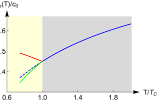
Figure 2: Kink in the $T$-dependence of the shear elastic constant $c_{s}(T)$ at a superconducting transition $T_{c}$. The system is close to a nematic instability and the nematic correlation length increases with lowering $T$. For sufficiently large $\lambda_{0}>0$ the elastic constant hardens immediately upon entering the superconducting phase (red/dark line), as seen in the Fe-based systems. For $\lambda_{0}<0$ the elastic constant softens more rapidly in the superconducting phase (green/light line). The dashed line is the extrapolation of the metallic behavior.

The enhancement of $\lambda$ implied by Eq. (6) has the following two consequences.

1. $c_{s}(T)$ across superconducting $T_{c}$. Since $\chi_{n}^{m}(T)\propto 1/(T-T_{0})$ while $\lambda_{\rm renorm}\propto 1/(T-T_{0})^{2}$ has a stronger $T$-dependence, it is clear that, for $\lambda_{0}$ above a positive threshold, the softening of $c_{s}(T)$ in the metal phase will turn into a hardening in the superconducting phase. This can be illustrated from the following phenomenological modeling. We write $c_{s}(T)/c_{0}=1-a_{0}P(T)/[1-b_{0}P(T)],$ where $a_{0}\equiv\alpha^{2}\mathcal{N}_{F}/c_{0}$ and $b_{0}\equiv g\mathcal{N}_{F}$ are constants, and $P(T)$ is the dimensionless bare nematic polarization. In the metallic phase we postulate $P(T\geq T_{c})=\Lambda/(T+T_{1})$, with $T_{1}\gg T_{c}$ such that $P(T)$ is weakly $T$-dependent around $T_{c}$. As noted above, in the superconducting phase the bare polarization has an additional term proportional to $\lambda_{0}\Delta(T)^{2}$. We assume the mean field scaling $\Delta(T)^{2}=\Delta_{0}^{2}(1-T/T_{c})$, and we write the bare interplay coupling $\lambda_{0}$ in terms of a dimensionless parameter $t_{2}\equiv\lambda_{0}\Delta_{0}^{2}/(\alpha^{2}\mathcal{N}_{F})$. This implies $P(T\leq T_{c})=\Lambda/(T+T_{1})-t_{2}(1-T/T_{c})$. It follows that, for sufficiently large and positive $t_{2}>\Lambda T_{c}/(T_{c}+T_{1})^{2}$, the elastic constant $c_{s}(T)$ starts hardening immediately below $T_{c}$, as seen in electron and holed doped BaFe₂As₂ fernandes-2010 ; yoshizawa ; boehmer-2014 ; boehmer-2016 . On the other hand, for $t_{2}<0$ (or equivalently $\lambda_{0}<0$) the elastic softening enhances in the superconducting phase. It is likely that this latter trend is relevant for FeSe_1-xS_x at large doping where $T_{c}>T_{s}$ wang-2016 . These two trends are illustrated in Fig. (2) for which we use $a_{0}=0.22$, $b_{0}=49.8$, $T_{1}/\Lambda=50$, $T_{c}/\Lambda=0.2$, while $t_{2}=1.3\times 10^{-4}$ and $t_{2}=-0.2\times 10^{-4}$ for the red (dark) and green (light) lines, respectively. For intermediate values of $t_{2}$ the $T$-dependence of $c_{s}(T)$ interpolates between these two limiting behaviors.

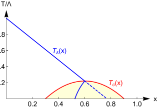
Figure 3: Back-bending of the nematic transition line (solid blue line) $T_{s}(x)$ in the superconducting phase (shaded light yellow) due to strong interplay between the two orders. The blue dashed line is the hypothetical nematic transition if the interplay is ignored.

2. Back-bending of $T_{s}(x)$ in the superconducting phase. As noted above, for $\lambda_{0}$ greater than a positive threshold the shear modulus $c_{s}(T)$ hardens for $T\leq T_{c}$ (red/dark line in Fig. (2)). An immediate consequence of this behavior is the back-bending of the nematic/orthorhombic transition line $T_{s}(x)$ in the superconducting phase, as shown in Fig. (3). Here $x$ is a hypothetical tuning parameter that, in practice, can be related to doping or pressure. To illustrate the back-bending we consider the same model of $P(T)$ as above, and we introduce an $x$-dependence to the temperature scales $T_{1}(x)/\Lambda=49.02+1.3x$ and $T_{c}(x)/\Lambda=0.22-2.44(x-0.6)^{2}$, and to the parameter $t_{2}(x)=3\times 10^{-3}[T_{c}(x)/\Lambda]^{2}$. Thus, in this model $T_{c}(x)$ has a dome-like structure, and the $T_{s}(x)$ is linearly decreasing with $x$. The two transition lines meet at $x=0.6$, and if the interplay is ignored $T_{s}(x)$ continues the trend (dashed lines Fig. (3)) in the superconducting phase. However, once the interplay is taken into account, the hardening of $c_{s}(T)$ for $T<T_{c}$ implies that there cannot be a nematic transition for $x>0.6$ in the superconducting phase. Moreover, since the hardening increases with lowering $T$, it necessarily implies that $T_{s}(x)$ back-bends in the superconducting phase, as reported in electron-doped BaFe₂As₂ nandi2010 .

To summarize, we examined the thermodynamic signatures of the interplay between superconducting and nematic instabilities. In particular, we studied microscopically the properties of the coupling $\lambda$ between the two orders, see Eq. (1). This is related to how the shear elastic constant $c_{s}(T)$ changes across a superconducting transition. We explained why in most systems $\lambda$ (in suitable unit) is small and nearly temperature independent, which leads to $\delta c_{s}/|c_{s}^{m}|\sim 10^{-6}$ as seen in most classes of superconductors. The situation is different if, due to an imminent nematic instability, the nematic correlation length $\xi\gg l$, where $l$ is the interatomic distance. In this case $\lambda\propto(\xi(T)/l)^{4}$ has strong $T$-dependence and it can be boosted by several orders of magnitude. This leads to large $\delta c_{s}/|c_{s}^{m}|\sim 10^{-1}$, as seen experimentally in the Fe-based and A15 superconductors. If the bare coupling $\lambda_{0}$ is above a positive threshold, it leads to hardening of $c_{s}(T)$ for $T\leq T_{c}$, and to the back-bending of the nematic transition line in the superconducting phase, as seen in doped BaFe₂As₂. Finally, we predict that the A15 systems have large electronic nematic correlation which can be revealed using electronic Raman response and elastoresistivity techniques.

- (1) For reviews see, e.g., M. Norman, Physics 1, 21 (2008); D. C. Johnston, Adv. Phys. 59, 803 (2010); G. R. Stewart, Rev. Mod. Phys. 83, 1589 (2011); P. J. Hirschfeld, M. M. Korshunov, and I. I. Mazin, Rep. Prog. Phys. 74, 124508 (2011); A. V. Chubukov, Annu. Rev. of Condens. Matter Phys. 3, 57 (2012).
- (2) H.-H. Kuo, J.-H. Chu, J. C. Palmstrom, S. A. Kivelson, and I. R. Fisher, Science 352, 958 (2016).
- (3) D. Chowdhury, E. Berg, and S. Sachdev, Phys. Rev. B 84, 205113 (2011); E.-G. Moon and S. Sachdev, Phys. Rev. B 85, 184511 (2012).
- (4) G. Livanas, A. Aperis, P. Kotetes, and G. Varelogiannis, Phys. Rev. B 91, 104502 (2015).
- (5) R. M. Fernandes and A. J. Millis, Phys. Rev. Lett. 111, 127001 (2013).
- (6) J. K. Glasbrenner, I. I. Mazin, H. O. Jeschke, P. J. Hirschfeld, and R. Valentí, Nat. Phys. 11, 953 (2015).
- (7) V. Mishra and P. J. Hirschfeld, New J. Phys. 18, 103001(2016).
- (8) Y. Gallais, I. Paul, L. Chauvière, and J. Schmalian, Phys. Rev. Lett. 116, 017001 (2016).
- (9) P. O. Sprau, A. Kostin, A. Kreisel, A. E. Böhmer, V. Taufour, P. C. Canfield, S. Mukherjee, P. J. Hirschfeld, B. M. Andersen, and J. C. Séamus Davis, Science 357, 75 (2017).
- (10) D. D. Scherer, A. C. Jacko, C. Friedrich, E. Şaşioğlu, Stefan Blügel, R. Valentí, and B. M. Andersen, Phys. Rev. B 95, 094504 (2017).
- (11) L. Classen, R.-Q. Xing, M. Khodas, A. V. Chubukov, Phys. Rev. Lett. 118, 037001 (2017).
- (12) L. Benfatto, B. Valenzuela, and L. Fanfarillo, npj Quantum Materials 3, 56 (2018).
- (13) Y. Ando, K. Segawa, S. Komiya, and A. N. Lavrov, Phys. Rev. Lett. 88, 137005 (2002).
- (14) C. Howald, H. Eisaki, N. Kaneko, M. Greven, and A. Kapitulnik, Phys. Rev. B 67, 014533 (2003).
- (15) V. Hinkov, D. Haug, B. Fauqué, P. Bourges, Y. Sidis, A. Ivanov, C. Bernhard, C. T. Lin, and B. Keimer, Science 319, 597 (2008).
- (16) R. Daou, J. Chang, David LeBoeuf, Olivier Cyr-Choinière, Francis Laliberté, Nicolas Doiron-Leyraud, B. J. Ramshaw, R. Liang, D. A. Bonn, W. N. Hardy, and Louis Taillefer, Nature 463, 519 (2010).
- (17) Y. Sato, S. Kasahara, H. Murayama, Y. Kasahara, E.-G. Moon, T. Nishizaki, T. Loew, J. Porras, B. Keimer, T. Shibauchi and Y. Matsuda, Nat. Phys. 13, 1074 (2017).
- (18) N. Auvray, S. Benhabib, M. Cazayous, R. D. Zhong, J. Schneeloch, G. D. Gu, A. Forget, D. Colson, I. Paul, A. Sacuto, and Y. Gallais, arXiv:1902.03508.
- (19) S. A. Kivelson, I. P. Bindloss, E. Fradkin, V. Oganesyan, J. M. Tranquada, A. Kapitulnik, and C. Howald, Rev. Mod. Phys. 75, 1201 (2003).
- (20) M. Vojta, Adv. Phys. 58, 699 (2009).
- (21) J. Wang and G.-Z. Liu, New J. Phys. 15, 073039 (2013).
- (22) H. Yamase and R. Zeyher, Phys. Rev. B 88, 180502(R) (2013).
- (23) T. A. Maier, and D. J. Scalapino, Phys. Rev. B 90, 174510 (2014).
- (24) M. A. Metlitski, D. F. Mross, S. Sachdev, T. Senthil, Phys. Rev. B 91, 115111 (2015).
- (25) S. Lederer, Y. Schattner, E. Berg, and S. A. Kivelson, Phys. Rev. Lett. 114, 097001 (2015).
- (26) D. Labat and I. Paul, Phys. Rev. B 96, 195146 (2017).
- (27) A. Klein, Y.-M. Wu, A. Chubukov, arXiv:1812.00521
- (28) S. Lederer, E. Berg, and E.-A. Kim, arXiv:1908.03224.
- (29) R. M. Fernandes, L. H. VanBebber, S. Bhattacharya, P. Chandra, V. Keppens, D. Mandrus, M. A. McGuire, B. C. Sales, A. S. Sefat, and J. Schmalian, Phys. Rev. Lett. 105, 157003 (2010).
- (30) R. M. Fernandes, A. V. Chubukov, and J. Schmalian, Nat. Phys. 10, 97 (2014).
- (31) Y. Gallais and I. Paul, C. R. Phys. 17, 113 (2016).
- (32) Y. S. Kushnirenko, D. V. Evtushinsky, T. K. Kim, I.V. Morozov, L. Harnagea, S. Wurmehl, S. Aswartham, A.V. Chubukov, and S. V. Borisenko, arXiv:1810.04446.
- (33) J. L. Olsen, Nature 175, 37 (1955).
- (34) G. A. Alers and D. L. Waldorf, Phys. Rev. Lett. 6, 677 (1961).
- (35) M. Nohara, T. Suzuki, Y. Maeno, T. Fujita, I. Tanaka and H. Kojima, Phys. Rev. B 52, 570 (1995).
- (36) G. Bruls, D. Weber, B. Wolf, P. Thalmeier, and B. Lüthi, Phys. Rev. Lett. 65, 2294 (1990).
- (37) P. Thalmeier, B. Wolf, D. Weber, G. Bruls, B. Lüthi, and A. A. Menovsky, Physica C 175, 61 (1991).
- (38) L. R. Testardi, Phys. Rev. B 12, 3849 (1975).
- (39) A. J. Millis and K. M. Rabe, Phys. Rev. B 38, 8908 (1988).
- (40) M. Yoshizawa and S. Simayi, Mod. Phys. Lett. 26, 1230011 (2012).
- (41) G. A. Zvyagina, T. N. Gaydamak, K. R. Zhekov, I. V. Bilich, V. D. Fil, D. A. Chareev, and A. N. Vasiliev, EPL 101, 56005 (2013).
- (42) A. E. Böhmer, P. Burger, F. Hardy, T. Wolf, P. Schweiss, R. Fromknecht, M. Reinecker, W. Schranz, C. Meingast, Phys. Rev. Lett. 112, 047001 (2014).
- (43) A. E. Böhmer and C. Meingast, C. R. Physique 17, 90 (2016).
- (44) L. R. Testardi and T. B. Bateman, Phys. Rev. 154, 402 (1967).
- (45) W. Rehwald, M. Rayl, R. W. Cohen, and G. D. Cody, Phys. Rev. B 6, 363 (1972).
- (46) L. R. Testardi, Rev. Mod. Phys. 47, 637 (1975).
- (47) T. Koyama, Phys. Rev. B 70, 226503 (2004).
- (48) e.g., see A. A. Abrikosov, L. P. Gorkov, and I. E. Dzyaloshinski, Methods of Quantum Field Theory in Statistical Physics, Dover Publications Inc., New York (1975), chapter 2, pp. 77-78.
- (49) J.-H. Chu, H.-H. Kuo, J. G. Analytis, I. R. Fisher, Science 337, 710 (2012).
- (50) Y. Gallais, R. M. Fernandes, I. Paul, L. Chauvière, Y.-X. Yang, M.-A. Méasson, M. Cazayous, A. Sacuto, D. Colson, and A. Forget, Phys. Rev. Lett. 111, 267001 (2013).
- (51) V. K. Thorsm lle, M. Khodas, Z. P. Yin, C. Zhang, S. V. Carr, P. Dai, and G. Blumberg, Phys. Rev. B 93, 054515 (2016).
- (52) D. Steffensen, P. Kotetes, I. Paul, and B. M. Andersen, Phys. Rev. B 100, 064521 (2019).
- (53) L. Wang, F. Hardy, T. Wolf, P. Adelmann, R. Fromknecht, P. Schweiss, and C. Meingast, Phys. Status Solidi B 254, 1600153 (2017).
- (54) S. Nandi, M. G. Kim, A. Kreyssig, R. M. Fernandes, D. K. Pratt, A. Thaler, N. Ni, S. L. Bud ko, P. C. Canfield, J. Schmalian, R. J. McQueeney, and A. I. Goldman, Phys. Rev. Lett. 104, 057006 (2010).