A Locally Adaptive Bayesian Cubature Method

Abstract

Bayesian cubature (BC) is a popular inferential perspective on the cubature of expensive integrands, wherein the integrand is emulated using a stochastic process model. Several approaches have been put forward to encode sequential adaptation (i.e. dependence on previous integrand evaluations) into this framework. However, these proposals have been limited to either estimating the parameters of a stationary covariance model or focusing computational resources on regions where large values are taken by the integrand. In contrast, many classical adaptive cubature methods focus computational resources on spatial regions in which local error estimates are largest. The contributions of this work are three-fold: First, we present a theoretical result that suggests there does not exist a direct Bayesian analogue of the classical adaptive trapezoidal method. Then we put forward a novel BC method that has empirically similar behaviour to the adaptive trapezoidal method. Finally we present evidence that the novel method provides improved cubature performance, relative to standard BC, in a detailed empirical assessment.

1 Introduction

In this paper we consider the numerical approximation of the integral

$$I(f^{*})\coloneqq\int_{D}f^{*}(x)\,\mathrm{d}\pi(x),$$ (1)

of a continuous function $f^{*}:D\rightarrow\mathbb{R}$ with respect to a Borel reference measure $\pi$ supported on a compact set $D\subset\mathbb{R}^{d}$. In particular, we consider the case where the evaluation of $f^{*}$ is associated with a substantial computational cost. To control computational cost, a cubature method should attempt to control the number of evaluations of $f^{*}$ required to obtain a desired level of accuracy for (1). In particular, a desirable attribute of a cubature method is to focus integrand evaluations on subregions of $D$ in which the approximation of $f^{*}$ is most difficult. If the user has no a priori knowledge about the locations of such regions then the cubature algorithm must be locally adaptive if it is to fulfill this requirement. Furthermore, any practical cubature method should provide an estimate of its precision, such as an a posteriori error estimate if the cubature method is classical, or a credible interval if a probabilistic cubature method is used.

The Bayesian cubature (BC) method for approximation of (1) can be traced back to Larkin, (1972). Here, approximation of (1) is framed as an inferential task where the integrand $f^{*}$ carries the status of a latent variable to be inferred. A distinguishing feature of BC, compared to classical approaches, is that the output of the method is a probability distribution on $\mathbb{R}$, simultaneously providing estimates and quantification of uncertainty regarding the value of the integral (1). The method finds application in machine learning (Osborne et al.,, 2012), statistics (Briol et al.,, 2019), signal processing (Prüher et al.,, 2018) and econometrics (Oettershagen,, 2017), most typically in situations where evaluation of the integrand $f^{*}$ is associated with a substantial computational cost. In the context of uncertainty quantification, for example, it becomes natural and parsemonious to combine the probabilistic output provided by BC with other probabilistic representations of uncertainty, such as measurement error and model error.

The general framework for BC can be expressed using two ingredients, the first of which is an underlying probability space $(\Omega,\mathcal{F},\mathbb{P})$ on which a stochastic process $f:D\times\Omega\rightarrow\mathbb{R}$ is defined. This serves as a statistical model for the latent $f^{*}$ and is endowed with the Bayesian semantics of a priori knowledge about the integrand. For instance, global properties, such as periodicity or monotonicity, and local properties, such as continuity and differentiability, may be known a priori and encoded. It is minimally required that sample paths of $f$ are continuous and that $f$ admits well-defined conditional processes, denoted $f|\mathcal{D}_{n}$, whenever $\mathcal{D}_{n}=\{(x_{i},f^{*}(x_{i}))\}_{i=1}^{n}$ specifies $n$ evaluations of the integrand on which the process is conditioned. Thus, in particular, the stochastic process $f$ can be integrated, giving rise to a random variable

$$I(f):\Omega \rightarrow \mathbb{R}$$

$$\omega \mapsto \int_{D}f(x,\omega)\,\mathrm{d}\pi(x).$$

The second ingredient is an acquisition function $A$, which – roughly speaking – maps a stochastic process (such as $f$) to a state $x\in D$. At iteration $n$ of a BC method, the acquisition function is applied to the conditional process $f|\mathcal{D}_{n-1}$ and the output $x_{n}\in D$ represents the location where the integrand is next evaluated. The conditional process $f|\mathcal{D}_{n}$ can be integrated to produce a random variable $I(f)|\mathcal{D}_{n}$ on $\mathbb{R}$, whose distribution is the posterior marginal distribution for the integral (1); this is the output of the BC method. Note that we do not mandate a stopping rule based on an error estimate as part of a BC method; we are motivated by problems where $f^{*}$ is associated with a substantial computational cost, so that one cannot practically expect to evaluate the integrand as many times as needed to achieve a pre-specified error threshold.

Through the choice of the stochastic process $f$ and the acquisition function $A$, the behaviour of the BC method can be controlled. Here we overview existing work on BC, in terms of the framework just set out. Attention is limited to approaches that select the $x_{i}$ according to some optimality criterion, as opposed to a set or sequence of $x_{i}$ being a priori posited (for a discussion of the latter context, which has also been widely-studied, see Briol et al.,, 2019; Jagadeeswaran and Hickernell,, 2019). The symbols $\mathbb{E}$, $\mathbb{V}$ and $\mathbb{C}$ are used to denote expectation, variance and covariance with respect to the underlying prior measure $\mathbb{P}$.

Non-Adaptive BC:

The earliest contributions to this area, from Sul’din, (1959, 1960); Larkin, (1974); Diaconis, (1988) and O’Hagan, (1991), considered a Gaussian stochastic process model $f\sim\mathcal{GP}(m,k)$ for the integrand, with mean function $m(x)=\mathbb{E}[f(x)]$ and covariance function $k(x,y)=\mathbb{C}[f(x),f(y)]$ being a priori specified (Rasmussen and Williams,, 2006). It can be shown that $\mathbb{V}[I(f)|\mathcal{D}_{n}]$, the posterior variance of the integral, depends on $\mathcal{D}_{n}$ only through the locations $x_{i}$ and not the actual values $f^{*}(x_{i})$ obtained. Thus the posterior variance can be arbitrarily small whilst the actual error can be arbitrarily large. These aforementioned authors proposed to select the $x_{i}$ in a manner that minimises $\mathbb{V}[I(f)|\mathcal{D}_{n}]$, and as such no adaptation is achieved. Indeed, in those references the $\{x_{i}\}_{i=1}^{n}$ were pre-computed to globally minimise $\mathbb{V}[I(f)|\mathcal{D}_{n}]$ over the product space $D^{n}$, though we note that sequential (greedy) alternatives have been studied in Oettershagen, (2017); Pronzato and Zhigljavsky, (2018).

Globally Adaptive BC:

Subsequent authors considered parametric families of stationary Gaussian processes $f|\theta\sim\mathcal{GP}(m_{\theta},k_{\theta})$, where $k_{\theta}$ has the form $k_{\theta}(x,y)=\phi_{\theta}(\|x-y\|)$, $\phi_{\theta}:[0,\infty)\rightarrow\mathbb{R}$ (e.g. $\phi_{\theta}(s)=\theta_{1}^{2}e^{-s^{2}/\theta_{2}^{2}}$), considering the parameter $\theta=(\theta_{1},\theta_{2})$ as a latent variable to also be inferred. This additional flexibility allows $\mathbb{V}[I(f)|\mathcal{D}_{n}]$ to depend on $\{f^{*}(x_{i})\}_{i=1}^{n}$ and so some form of adaptivity may be achieved when, for example, the minimum expected variance acquisition function

$$A(f|\mathcal{D}_{n-1})\in\operatorname*{arg\,min}_{x_{n}\in D}\mathbb{E}[\mathbb{V}[I(f)|\tilde{\mathcal{D}}_{n}]|\mathcal{D}_{n-1}]$$ (2)

is used. Here $\mathbb{E}[\cdot|\mathcal{D}_{n-1}]$ denotes expectation with respect to $f|\mathcal{D}_{n-1}$ and $\tilde{\mathcal{D}}_{n}=\mathcal{D}_{n-1}\cup\{(x_{n},f(x_{n}))\}$. In other words, $x_{n}$ is selected to minimise the expectation of $\mathbb{V}[I(f)|\tilde{\mathcal{D}}_{n}]$ when the random variable $f(x_{n})$ is distributed according to its marginal under $f|\mathcal{D}_{n-1}$. Adaptive selection of the $x_{i}$ in this context was studied in Osborne, (2010). The stationary (i.e. global) nature of the covariance model $\phi_{\theta}$ has the limitation that the resulting set $\{x_{i}\}_{i=1}^{n}$ tends to focus equally on regions where the integrand is both well and not well approximated. Indeed, inferences for the parameter $\theta$ are principally driven by the “most difficult” part of the integrand, even if that region is spatially localised. Thus any stopping rule based on the posterior variance of the integral results in unnecessary computational effort devoted to regions in which the integrand can be easily approximated.

Locally Adaptive BC:

The transformed stochastic process model $f(x,\omega)=T(g(x,\omega))$, where $T:\mathbb{R}\rightarrow\mathbb{R}$ is a pre-specified transformation and $g\sim\mathcal{GP}(m,k)$, has been proposed to encode global properties such as positivity (e.g. $T(z)=z^{2}$) into the stochastic process model. This was considered empirically in Gunter et al., (2014); Chai and Garnett, (2019) and theoretically in Kanagawa and Hennig, (2019). Coupled with the acquisition function (2), this construction behaves in such a way that regions in which $f^{*}(>0)$ is large are allocated more of the computational budget. Though appropriate in some situations (in particular, computation of marginal likelihood), such behaviour is not universally desirable (for instance, if $f^{*}$ is easily approximated in the regions where $f^{*}$ is large then such a strategy is likely to be inefficient).

Despite this extensive research development, the basic notion of allocating more computational resource to regions where approximation of the integrand is most difficult has not yet been realised in the context of a BC method. It is emphasised that adaptivity in this sense is ubiquitous throughout classical numerical analysis; for instance QUADPACK (Piessens,, 1983) has been a standard integration library since its inception and all but one of its integration routines are adaptive. In addition, for sufficiently challenging integration problems it is known, both theoretically (Ritter,, 2000, Chap. VII.3) and empirically (Rabe-Hesketh et al.,, 2002), that local adaptation is practically essential. It is therefore interesting and important to ask whether local adaptivity can also be exhibited by a suitably-designed BC method.

Outline:

Our contributions in this paper are three-fold: After recalling the classical adaptive trapezoidal method in Section 2 we then present a theoretical result, in Section 3, that suggests there does not exist a direct Bayesian analogue of this classical method. Then, in Section 4 we put forward a novel BC method that has empirically similar behaviour to the adaptive trapezoidal method. Its performance is empirically assessed in Section 5.

2 Background

In Section 2.1 the classical adaptive approach to cubature is briefly recalled, while standard background on the BC method is contained in Section 2.2.

2.1 Classical Adaptive Cubature

Classical approaches to (non-adaptive, for the moment) cubature can be categorised either as non-constructive (e.g. Monte Carlo, quasi Monte Carlo) or constructive (e.g. Newton-Cotes rules, Gaussian cubature). The latter are distinguished by the fact that they first construct an approximation to the integrand itself, typically an interpolant, and then exactly integrate this interpolant to obtain an approximation of (1). In either case, for a linear cubature method the output is an approximation

$$Q_{n}(f^{*})\coloneqq\sum_{i=1}^{n}w_{i}f^{*}(x_{i})\approx\int_{D}f^{*}(x)\,\mathrm{d}\pi(x)$$ (3)

based on a set $\{x_{i}\}_{i=1}^{n}\subset D$ that must be specified. The point estimate $Q_{n}(f^{*})$ is accompanied by an assessment of its error, $\epsilon=|I(f^{*})-Q_{n}(f^{*})|$, typically formulated as the difference $\tilde{\epsilon}=|Q_{n}(f^{*})-Q_{m}(f^{*})|$ of two cubature rules (though we note that more general approaches based on extrapolation are also used; Richardson and Gaunt,, 1927).

The classical notion of local adaptivity is to recursively partition the integration domain $D=\cup_{r=1}^{R}D_{r}$ into sub-regions $D_{r}$ over which local cubature rules of the form (3) are applied. An estimate $\tilde{\epsilon}_{r}$ of the error $\epsilon_{r}$ of these rules is produced for each region $D_{r}$ and, if the estimated error is too big, those regions are sub-divided again until a global error tolerance $\sum_{r=1}^{R}\tilde{\epsilon}_{r}<\tau$ is satisfied. Several such methods have been proposed, see Gonnet, (2012). For example, recall the trapezoidal rule on $D=[a,b]$ with $\mathrm{d}\pi(x)=\mathrm{d}x$, which has the form,

$$\texttt{Trap}(f^{*},a,b,n) \vcentcolon=\frac{b-a}{2n}\left(f^{*}(a)+f^{*}(b)+2\sum_{i=1}^{n-1}f^{*}\left(a+\frac{i(b-a)}{n}\right)\right).$$ (4)

The trapezoidal rule forms the basis for the classical locally adaptive trapezoidal method:

Algorithm 1 Adaptive Trapezium Method

1:procedure AdapTrap${}_{\rho,m,k}(f^{*},a,b,\tau)$

2:   $Q_{1}\leftarrow\texttt{Trap}(f^{*},a,b,m)$

3:   $Q_{2}\leftarrow\texttt{Trap}(f^{*},a,b,2m)$

4:   $\tilde{\epsilon}\leftarrow|Q_{2}-Q_{1}|$

5:   if $\tilde{\epsilon}<\tau$ then

6:      $\hat{I}\leftarrow Q_{2}$

7:   else

8:      $\tau^{\prime}\leftarrow\rho\tau$

9:      $\hat{I}\leftarrow\sum_{i=0}^{l-1}\texttt{AdapTrap}_{\rho,m,k}\left(f^{*},a+\frac{(b-a)i}{k},a+\frac{(b-a)(i+1)}{k},\tau^{\prime}\right)$    

10:   return $\hat{I}$

The AdapTrap method is an adaptive trapezoidal rule where the decision to subdivide into $k$ uniform intervals is determined by the difference between the composite trapezoidal rule on $2m$ intervals and the composite trapezoidal rule on $m$ intervals. The values $\tilde{\epsilon}$ thus form local error estimates and we accept our trapezoidal approximation to the integral on the subinterval only when $\tilde{\epsilon}$ is sufficiently small. The parameter $\rho$ controls how the error tolerance $\tau$ scales at each recursive step of the algorithm and has natural choice $\rho=\frac{1}{k}$.

Generalisation of the AdapTrap algorithm is straight-forward through the use of higher-order cubature rules (e.g. Simpson’s rule or Gaussian quadrature) within each step of the procedure (Davis and Rabinowitz,, 1984; Kahaner and Rechard,, 1987; Berntsen et al.,, 1991). It is intuitively clear that any such method will attempt to allocate computational resources to those regions where approximation of $f^{*}$ is most difficult. As argued in Section 1, this is not a feature of any existing BC method.

2.2 Standard Bayesian Cubature

In this section we briefly recall the pertinent aspects of the standard BC method.

Notation

Let $f_{X}^{*}$ with $[f_{X}^{*}]_{i}=f^{*}(x_{i})$ contain evaluations of the integrand on the ordered $n$-tuple $X=(x_{1},\ldots,x_{n})\in D^{n}$. For $k:D\times D\rightarrow\mathbb{R}$ and $Y=(y_{1},\ldots,y_{m})\in D^{m}$, the matrix $K_{XY}$ is defined as $[K_{XY}]_{ij}\vcentcolon=k(x_{i},y_{j})$. Let also $K_{X}(y)$ be defined as $[K_{X}(y)]_{i}\vcentcolon=k(x_{i},y)$ whenever $y\in D$. The equivalent presentations of stochastic processes $f:D\times\Omega\rightarrow\mathbb{R}$ and $f(x):\Omega\rightarrow\mathbb{R}$ are used, so that $f_{X}$ where $[f_{X}]_{i}=f(x_{i})$ is a random vector in $\mathbb{R}^{n}$.

Recall that a stochastic process $f$ is Gaussian if and only if, for any $X\in D^{n}$, $n\in\mathbb{N}$, the random vector $f_{X}$ is Gaussian-distributed. Thus a Gaussian process $f$ is completely specified by its mean function $m(x)\vcentcolon=\mathbb{E}[f(x)]$ and covariance function $k(x,y)\vcentcolon=\mathbb{C}[f(x),f(y)]$ and we write $f\sim\mathcal{GP}(m,k)$. Under mild regularity conditions (which are beyond the scope of this work to discuss in detail; see Bogachev,, 1998) it can be shown that the conditional stochastic processes $f|\mathcal{D}_{n}$ are well-defined, are also Gaussian, and have mean and covariance functions

$$m_{\mathcal{D}_{n}}(x) =f_{X}^{*\top}K_{XX}^{-1}K_{X}(x),$$ (5)

$$k_{\mathcal{D}_{n}}(x,y) =k(x,y)-K_{X}(x)^{\top}K_{XX}^{-1}K_{X}(y).$$ (6)

The output of the BC method is the random variable $I(f)|\mathcal{D}_{n}\sim\mathcal{N}(\mu_{n},\sigma_{n}^{2})$, which can be read off (5) and (6) as a univariate marginal:

$$\mu_{n} = \int_{D}m_{\mathcal{D}_{n}}(x)\,\mathrm{d}\pi(x)$$ (7)

$$= f_{X}^{*\top}K_{XX}^{-1}\int_{D}K_{X}(x)\,\mathrm{d}\pi(x),$$

$$\sigma_{n}^{2} = \int_{D}\int_{D}k_{\mathcal{D}_{n}}(x,y)\,\mathrm{d}\pi(x)\mathrm{d}\pi(y)$$ (8)

$$= \int_{D}\int_{D}k(x,y)\,\mathrm{d}\pi(x)\,\mathrm{d}\pi(y)-\left[\int_{D}K_{X}(x)\,\mathrm{d}\pi(x)\right]^{\top}K_{XX}^{-1}\left[\int_{D}K_{X}(y)\,\mathrm{d}\pi(y)\right].$$

The posterior mean (7) is seen to have the same form as (3). It is natural to select the design $X$ in such a way that the posterior variance (8) is minimised. Since (8) does not depend on $f^{*}$, no adaptive estimation occurs in the standard BC method and the assessment of uncertainty provided by (8) is exclusively driven by the a priori specification of $k$ and $X$. This behaviour is unsatisfactory, as posterior variance can be arbitrarily small whilst the actual error can be arbitrarily large. However, this property does allow optimal designs $X$ to, in principle, be pre-computed (Sul’din,, 1959, 1960; O’Hagan,, 1991; Minka,, 2000). Strategies to ensure analytic expressions for the integrals in (7) and (8) were proposed in Briol et al., (2019); Jagadeeswaran and Hickernell, (2019). For large $n$, techniques have been put forward to facilitate the efficient inversion of the matrix $K_{XX}$ (Karvonen and Särkkä,, 2018; Karvonen et al.,, 2019; Jagadeeswaran and Hickernell,, 2019).

Proposals that go beyond the standard BC method were outlined in Section 1. The simplest route to adaptivity is to consider a parametric family of covariance functions $k_{\theta}$ and to treat the parameter $\theta$ also as a latent variable to be inferred. For example, if $k_{\theta}(x,y)=\theta_{1}^{2}e^{-\|x-y\|^{2}/\theta_{2}^{2}}$ with $\theta=(\theta_{1},\theta_{2})$, then estimation of $\theta_{1}$ corresponds (roughly speaking) to estimating the amplitude of the integrand, while $\theta_{2}$ corresponds to a characteristic lengthscale for the integrand. This form of adaptation (which may be realised either through full Bayesian inference for $\theta$ or as an empirical Bayes method) was first empirically demonstrated to produce reliable uncertainty assessment in Larkin, (1974). However, the stationary form of the covariance model (i.e. the fact that two parameters $\theta_{1}$ and $\theta_{2}$ are required to describe the entire integrand) precludes the focussing of computational resources on those regions in which approximation of the integrand is most difficult. As a result, for integrands involving spatially-localised variation, existing BC methods based on a stationary covariance model can be arbitrarily inefficient in terms of the number of evaluations of the integrand.

All existing work on the BC method, with the exception of the transformed stochastic process models of Gunter et al., (2014); Chai and Garnett, (2019); Kanagawa and Hennig, (2019), have been based upon a stationary covariance model. Thus, in particular, no Bayesian analogues of classical locally adaptive methods have been proposed. In the next section we establish a cautionary result on the difficulties in developing a Bayesian analogue of the adaptive trapezoidal method. This serves as motivation for our novel proposal in Section 4.

3 A Bayesian AdapTrap?

The aim of this section is to discuss how one might naively attempt to create a direct Bayesian analogue of AdapTrap. To this end we recall the approach of Diaconis, (1988), who took a classical cubature rule of the form (3) and asked “for what prior does (3) arise as the mean of the posterior marginal distribution of the integral?”. Thus, in the context of creating an analogue of AdapTrap, we can follow Diaconis and seek a prior such that the mean of the posterior marginal for the integral is Trap in (4). Thus we must consider stochastic processes for which the conditional mean is the piecewise linear interpolant (over the range of $x_{1},\dots,x_{n}$) of the data $\mathcal{D}_{n}$ on which it is conditioned.

Let $C([a,b])$ denote the set of continuous real-valued functions on $[a,b]$ and consider the subset $F_{\rho,m,k,\tau}\subset C([a,b])$ of integrands $f^{*}$ for which AdapTrap_ρ,m,k fails to achieve its stated error tolerance $\tau$ upon termination, or for which AdapTrap_ρ,m,k fails to terminate at all (this set is non-empty; e.g. Clancy et al.,, 2014). From an inferential perspective, the decision to employ AdapTrap_ρ,m,k can be regarded as a belief that $f^{*}\notin F_{\rho,m,k,\tau}$. 3.1, presented next, suggests that stochastic process models giving rise to piecewise linear interpolants are incompatible with the use of AdapTrap_ρ,m,k, due to assigning non-zero probability mass to $F_{\rho,m,k,\tau}$ whenever $\tau>0$. This result, whose proof is straight-forward and contained in the supplement, can be interpreted as an average-case analysis of AdapTrap (Ritter,, 2000). Denote the error function $\text{erf}(x)\coloneqq\frac{1}{\sqrt{\pi}}\int_{-x}^{x}e^{-t^{2}}\,\mathrm{d}t$.

Proposition 3.1.

Fix $a<b$, $\rho>0$, $m\in\mathbb{N}$ and $k$ a positive even integer. Let $f^{*}$ be sampled from a centred Gaussian process on $C([a,b])$, whose law is denoted $\mathbb{P}^{*}$, such that the conditional mean $f^{*}|\mathcal{D}_{n}$ is the piecewise linear interpolant (over the range of $x_{1},\dots,x_{n}$) of the data $\mathcal{D}_{n}$ on which it is conditioned. If AdapTrap terminates, denote its error $\epsilon_{\rho,m,k,\tau}(f^{*})\vcentcolon=I(f^{*})-\texttt{AdapTrap}_{\rho,m,k}(f^{*},a,b,\tau)$, otherwise set $\epsilon_{\rho,m,k,\tau}(f^{*})\vcentcolon=\infty$. Then for every $\tau>0$,

$$\mathbb{P}^{*}(|\epsilon_{\rho,m,k,\tau}|>\tau)\;>\;\textstyle\text{erf}(c\tau)\left[1-\text{erf}(\sqrt{3}c\tau)\right],$$

where $c>0$ is a $\mathbb{P}^{*}$-dependent constant.

Though the probability mass assigned to $F_{\rho,m,k,\tau}$ can be made small, the fact that it is non-zero for all $\tau>0$ calls into doubt whether direct Bayesian analogues of classical adaptive methods can exist, in contrast to the situation for non-adaptive methods (Karvonen et al.,, 2018). In Section A.2, further average-case analysis is provided, showing that for mis-specified $\rho$ the expected number of steps of AdapTrap can be unbounded. Taken together, our analyses suggest that classical adaptive methods cannot be directly replicated in BC and a different strategy is needed. In Section 4 we therefore put forward a de novo BC method, which achieves adaptivity through a flexible non-stationary stochastic process model.

4 Adaptive Bayesian Cubature

The aim of this section is to develop a novel BC method that is locally adaptive, in the sense of focussing integrand evaluations on spatial regions where approximation of $f^{*}$ is most difficult. The forgoing discussion in Sections 1-3 suggests that this should be based on a non-stationary stochastic process model.

4.1 A Non-Stationary Process Model

Several non-stationary stochastic process models have been developed and in principle any of these could form the basis for a BC method. Three broad classes of non-stationary model are those based on deformation of the domain, partitioning of the domain, and convolution over the domain. The spatial deformation approach considers a stochastic process of the form $f(x,\omega)=g(v(x),\omega)$, where $g$ is a stationary stochastic process on $D$ and $v$ is a map from $D$ to itself. Such models are flexible but conditioning on data in this context can be computationally difficult. The joint estimation of $g$ and $v$ was considered in a frequentist context in Sampson and Guttorp, (1992) using thin-plate splines; analogous Bayesian approaches were developed in Damian et al., (2001); Schmidt and O’Hagan, (2003); Damianou and Lawrence, (2013). A Bayesian partition model represents a non-stationary process using piecewise stationary processes, each fitted on one element of a partition of $D$ (Kim et al.,, 2005; Gramacy and Lee,, 2008). The advantage of such a model is its simplicity and ease to fit, but an unfortunate consequence is that continuity of the process across elements of the partition is not easily enforced. The process convolution approach takes a collection of local covariance models and then – roughly speaking – convolves them to obtain a new, non-stationary global covariance model (Higdon et al.,, 1999; Paciorek,, 2003). Theoretical results on the flexibility of these models have been established (Dunlop et al.,, 2018).

The process convolution approach was used for the experiments in this paper. This choice allows for substantial flexibility to incorporate a priori knowledge and to adapt, in principle, to non-stationary features of the integrand. Following Paciorek, (2003), we adopted a hierarchical Gaussian process model with spatially-dependent lengthscale field. The first part of the model specifies that $f|\theta\sim\mathcal{GP}(m_{\theta},k_{\theta})$. The mean function $m_{\theta}=c$ is here taken as a constant $c\in\mathbb{R}$ and, letting $\phi:[0,\infty)\rightarrow\mathbb{R}$ be a positive definite radial basis function, the covariance function has the form

$$k_{\theta}(x,y)=\frac{\sigma^{2}\sqrt{\ell(x)\ell(y)}}{\sqrt{\ell(x)^{2}+\ell(y)^{2}}}\phi\left(\frac{\|x-y\|}{\sqrt{\ell(x)^{2}+\ell(y)^{2}}}\right).$$

The parameters to be jointly inferred are $\theta=\{c,\sigma,\ell(\cdot)\}$, where $\sigma>0$ is an amplitude parameter and $\ell:D\rightarrow[0,\infty)$ is a lengthscale field. The second part of the hierarchical model specifies a prior distribution for $\theta$. The lengthscale $\ell(\cdot)$ was itself parametrised as a piecewise linear and non-negative function throughout. Specific choices for $\phi$, the prior for $\theta$ and the parametrisation of $\ell(\cdot)$ are deferred to Section 5.

4.2 Adaptive Selection of the Point Set

A sequential approach to selecting the $x_{i}$ was adopted, based on the minimum expected variance acquisition function (2) of Osborne, (2010). This can be viewed as a specific instance of sequential Bayesian optimal experimental design (BOED; Chaloner and Verdinelli,, 1995). As is typical in BOED, (2) is an intractable global optimisation problem over $D$ that must in practice be approximated (e.g. Overstall et al.,, 2018). Two practical algorithms are now presented. In what follows we let $\mathcal{D}_{0}$ be pre-specified and let $D_{n}\subset D$ denote a finite set of reference points in $D$ over which the optimisation (e.g. grid search) required at stage $n$ of the algorithm is performed; full details are reserved for Appendix D. Recall that we do not mandate a stopping rule as part of a BC method. However, if required then the standard deviation of $I(f)|\mathcal{D}_{n}$ can be used to decide when the algorithm should be terminated. For completeness we present our algorithms with an explicit stopping rule included.

Algorithm 3, which is reserved for the supplement, uses Markov chain Monte Carlo (MCMC) to approximate the intractable acquisition function (2), in an idealised approach that we call AdapBC. The computational requirement of MCMC is assumed to be negligible compared to the cost of evaluating the integrand. However, the need to ensure convergence of the Markov chain introduces practical difficulties for the user and therefore we focus on an empirical Bayes (EB) alternative in Algorithm 2, called E-AdapBC, wherein the parameter $\theta$ is estimated rather than being marginalised. To avoid over-confident estimation, we regularised the EB estimator using an additional penalty term $r(\theta)$ specified in Appendix D. An advantage of E-AdapBC over AdapBC is that the computation of the expected variance in line 8 of Algorithm 2 has a closed form, vis a vis (8). This completes the methodological development; in the next section the proposed methods are empirically assessed.

Algorithm 2 (E) Adaptive Bayesian Cubature

1:procedure E-AdapBC($f^{*},\tau$)

2:   $n\leftarrow 1$, $\tilde{\epsilon}\leftarrow\infty$

3:   while $\tilde{\epsilon}\geq\tau$ do

4:      $\theta_{n}\leftarrow\operatorname*{arg\,max}_{\theta}p(\mathcal{D}_{n-1}\,|\,\theta)-r(\theta)$

5:      Sample $(f_{m})_{m=1}^{M}\sim f\,|\,\theta_{n},\mathcal{D}_{n-1}$ $\triangleright$ $M\gg 1$

6:      for each $x$ in $D_{n}$ do

7:         $\tilde{\mathcal{D}}_{n}\leftarrow\mathcal{D}_{n-1}\cup\{(x,f_{m}(x))\}$

8:         $E(x)\leftarrow\mathbb{E}[\mathbb{V}[I(f)|\theta_{n},\tilde{\mathcal{D}}_{n}]|\theta_{n},\mathcal{D}_{n-1}]$       

9:      Pick $x_{n}\in\operatorname*{arg\,min}_{x\in D_{n}}E(x)$

10:      $\mathcal{D}_{n}\leftarrow\mathcal{D}_{n-1}\cup\{(x_{n},f^{*}(x_{n})\}$

11:      $n\leftarrow n+1$, $\tilde{\epsilon}\leftarrow\mathbb{V}[I(f)|\theta_{n},\mathcal{D}_{n}]^{\frac{1}{2}}$    

12:   return $I(f)|\theta_{n},\mathcal{D}_{n}$

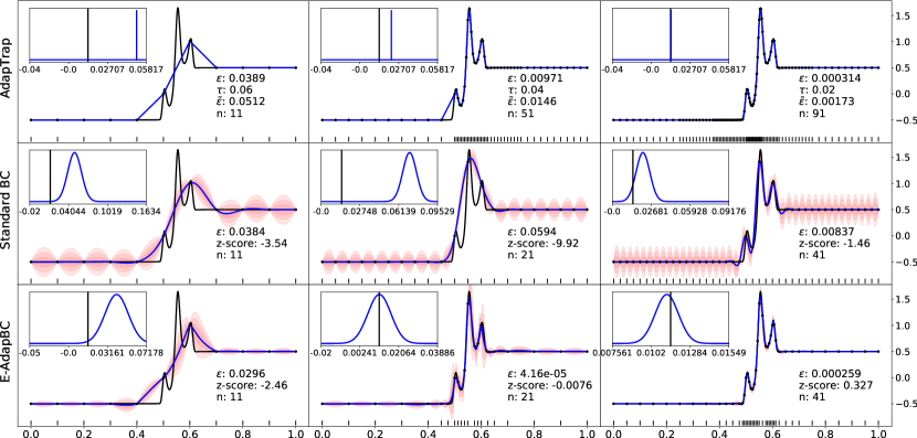
Figure 1: Comparison of AdapTrap, StdBC and E-AdapBC. [Here represents the true integrand $f^{*}$, represents the mean of the conditional process $f|\mathcal{D}_{n}$ and represents pointwise credible intervals. The tick marks indicate where the integrand was evaluated. For StdBC and E-AdapBC the error $\epsilon\vcentcolon=|\mu_{n}(f^{*})-I(f^{*})|$, the z-score $[\mu_{n}(f^{*})-I(f^{*})]/\sigma_{n}(f^{*})$ and the number of integrand evaluations $n$ are reported. For AdapTrap the error $\epsilon$, the global error tolerance $\tau$, the estimated error $\tilde{\epsilon}\vcentcolon=\sum_{r}\tilde{\epsilon}_{r}$ and the number of integrand evaluations $n$ are reported. Inset panels compare the true value $I(f^{*})\approx 0.011$ to the distribution $I(f)|\theta_{n},\mathcal{D}_{n}$. Settings for all methods are detailed in Appendix E.]

5 Experimental Assessment

The purpose of this section is to investigate whether (AdapBC and) E-AdapBC provide the local adaptation that is missing from standard BC. For the remainder, we use StdBC to signify the simplified version of E-AdapBC in which the lengthscale field $\ell(\cdot)$ is simply a constant, to be estimated. All other settings (e.g. the choice of $\phi$), were taken to be identical between StdBC and E-AdapBC. All methods that we consider incur an auxiliary computational cost that is orders of magnitude larger than that which would be associated with a classical cubature method. BC methods are motivated by situations where evaluation of $f^{*}$ is associated with a substantial computational cost (an explicit example is provided in Section 5.3), so that such auxiliary computation can be justified. For this reason, computational cost is quantified in the results that follow only through the number of evaluations of the integrand.

A BC method is considered to perform well if, loosely speaking, the posterior mean $\mu_{n}(f^{*})\vcentcolon=\mathbb{E}[I(f)|\theta_{n},\mathcal{D}_{n}]$ provides an accurate point estimate of (1) and the posterior spread $\sigma_{n}(f^{*})\vcentcolon=\mathbb{V}[I(f)|\theta_{n},\mathcal{D}_{n}]^{\frac{1}{2}}$ is well-calibrated as an indicator of the true error $|\mu_{n}(f^{*})-I(f^{*})|$; in this paper calibratedness is quantified by $Z_{n}(f^{*})\vcentcolon=\frac{\mu_{n}(f^{*})-I(f^{*})}{\sigma_{n}(f^{*})}$ whose values should be plausible as samples from $\mathcal{N}(0,1)$ when the BC method is well-calibrated (Briol et al.,, 2019). The ideas are illustrated next in Section 5.1. In Section 5.2 the results of detailed synthetic assessment are presented and in Section 5.3 we report results based on a realistic integration task involving trajectories of an autonomous robot. All results in this paper can be reproduced in Python using code available at github.com/MatthewAlexanderFisher/LocalABC.

5.1 Illustration of Adaptation

Figure 1 compares the performance of AdapTrap (top), StdBC (middle) and E-AdapBC (bottom) on a toy integrand $f^{*}$ in dimension $d=1$. Full details of the specific settings used for all methods are reserved for Section E.1. Theoretical analysis of StdBC indicates that the points $X$ at which the integrand is evaluated are essentially space-filling (Cor. 11 of Santin et al.,, 2017). In contrast, both AdapTrap and E-AdapBC deploy their computational resources in the region where $f^{*}$ is varying the most. AdapTrap provides an accurate point estimate for (1) and a deterministic error estimate $\tilde{\epsilon}$. In each case $\epsilon<\tau$, i.e. the true error has been controlled succesfully by AdapTrap. In contrast, both BC methods provide distributional output whose uncertainty is well-calibrated once $n$ is large enough that the regions of highest variation have been found. Of course, Figure 1 studies a single integrand and a more systematic assessment is performed next.

5.2 Synthetic Assessment

To assess the proposed methods on a wider range of test problems, we automatically generated integrands $f_{i}^{*}$, $i=1,\dots,100$, in a manner described in Section E.2. The negligible cost of evaluating the synthetic $f_{i}^{*}$ ensures that their integrals $I(f_{i}^{*})$ can be accurately approximated using a classical method, providing a gold-standard for assessment. The methods AdapBC and E-AdapBC were compared to StdBC. Figure 2 (top row) displays the mean of the relative errors $\left|\frac{\mu_{n}(f_{i}^{*})-I(f_{i}^{*})}{I(f_{i}^{*})}\right|$ for StdBC and E-AdapBC. Results are reported for the case $\mathrm{d}\pi(x)=\mathrm{d}x$ and in dimension $d=1$ (left) and $d=3$ (right). It can be seen that the conclusions of Figure 1 hold in broad terms over an ensemble of integrands, though of course there exist particular integrands for which StdBC happens due to chance to outperform E-AdapBC. The bottom row of Figure 2 reports coverage frequencies for the 95% highest-posterior density interval. Over-confidence is apparent at small values of $n$, especially for StdBC and for $d=3$, but for larger $n$ (when the most variable regions of the integrand are discovered) the methods are better calibrated. The impact of the choice of radial basis function $\phi(\cdot)$ and the parametrisation of the lengthscale field $\ell(\cdot)$ was investigated in Section E.3. Results for AdapBC were broadly similar to E-AdapBC after manual tuning of the MCMC and these are deferred to Section E.4.

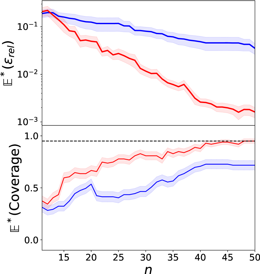
(a)

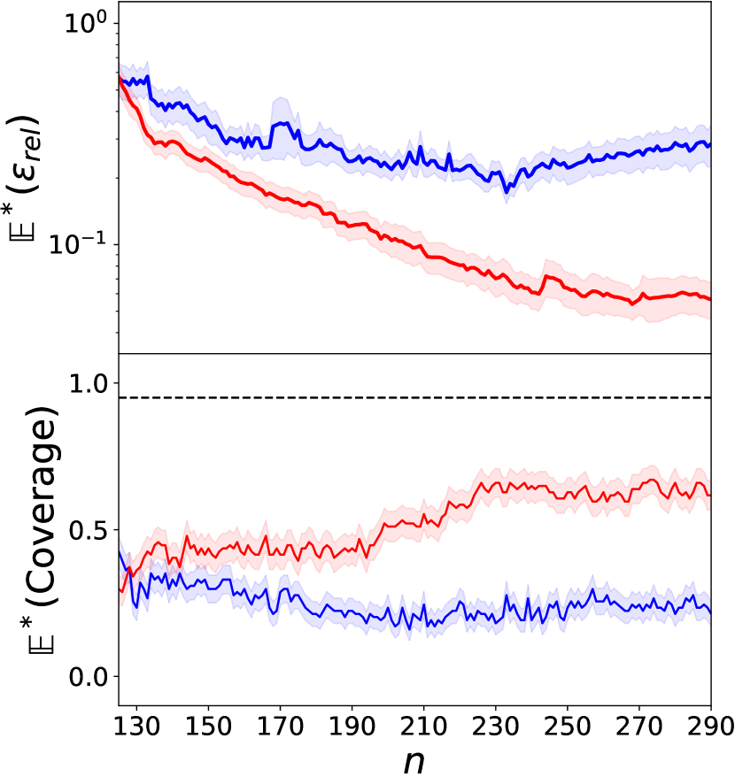
(b)

Figure 2: Synthetic assessment in (a) $d=1$ and (b) $d=3$ for StdBC ( ) and E-AdapBC ( ), where 100 integrands were randomly generated. Top row: the mean relative error against the number of evaluations $n$. Bottom row: the coverage frequencies for 95% credible intervals for each method. The notional coverage ( ) is indicated. [Standard errors displayed.]

5.3 Autonomous Robot Assessment

The final experiment concerns an application of E-AdapBC to autonomous robotics (Chrono, 2019a, ). Here $x\in\mathbb{R}^{3}$ represents parameters that describe the performance of a set of actuators in an autonomous walking robot. The notional value and actual value of $x$ will not be equal in general and there is interest in understanding the effect of parameter variability on the actual trajectory of the robot; see Figure 3(a). Let $(z_{1}(x),z_{2}(x))$ denote the spatial coordinates of the robot after a fixed sequence of commands have been completed. Conceptually, the variability in the parameters can be represented (after re-parametrisation) as $x\sim\mathcal{N}(0,I_{3\times 3})$ and there is interest in evaluating moments $I(f^{*})$ where $f^{*}\in\{z_{1},z_{2},z_{1}^{2},z_{2}^{2}\}$. The situation typifies instances where $f^{*}$ is associated with a substantial computational cost, since simulation of the robot moving requires the numerical solution of a system of ordinary differential equations. The methods StdBC and E-AdapBC were each applied to this task, with full details contained in Section E.5. The intractability of the true integrals $I(f^{*})$ precludes a direct assessment as in Section 5.2. Instead, we focus on estimation accuracy (only) and report an approximate bound based on Jensen’s inequality and Monte Carlo:

$$\mathbb{E}[(I(f)-I(f^{*}))^{2}|\theta_{n},\mathcal{D}_{n}] \;\leq\;\mathbb{E}[I((f-f^{*})^{2})|\theta_{n},\mathcal{D}_{n}]$$

$$=\;\int_{D}\mathbb{E}[(f(x)-f^{*}(x))^{2}|\theta_{n},\mathcal{D}_{n}]\mathrm{d}\pi(x)$$

$$\approx\;\frac{1}{m}\sum_{i=1}^{m}\mathbb{E}[(f(y_{i})-f^{*}(y_{i}))^{2}|\theta_{n},\mathcal{D}_{n}]$$ (9)

where $y_{i}\stackrel{{\scriptstyle\text{iid}}}{{\sim}}\mathcal{N}(0,I_{d\times d})$ and $m=264$. For each integrand, E-AdapBC outperformed StdBC as quantified by (9); see Figure 3(b).

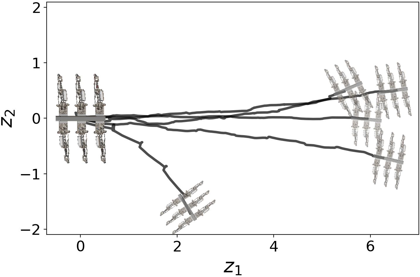
(a)

	Mean Sq. Error (9)
$f^{*}$	StdBC	E-AdapBC
$z_{1}$	$\underset{\pm 0.07}{0.895}$	$\underset{\pm 0.03}{\bf 0.293}$
$z_{2}$	$\underset{\pm 2.05}{14.3}$	$\underset{\pm 0.26}{\bf 2.28}$
$z_{1}^{2}$	$\underset{\pm 0.11}{0.884}$	$\underset{\pm 0.07}{\bf 0.336}$
$z_{2}^{2}$	$\underset{\pm 268.13}{1527}$	$\underset{\pm 11.13}{\bf 132.13}$

(b)

Figure 3: Autonomous robot assessment. (a) Trajectories produced by the robot. (b) Error as quantified in (9), for each of integrand $f^{*}$ relating to the final position of the robot. [Standard errors displayed.]

6 Conclusion

This paper highlighted the important issue of local adaptivity in the context of BC methods and discussed why naive constructions based on lifting classical adaptive methods to the Bayesian framework can fail. To address these issues, a novel locally adaptive BC method was proposed and demonstrated to perform well in both a synthetic and realistic empirical assessment. The construction was quite general, in the sense that essentially any sufficiently flexible Bayesian regression model can be used, and investigation of alternative regression models can form the basis of further work. Also of interest, non-myopic alternatives to (2) have been proposed for BC (Jiang et al.,, 2019) and these could also be investigated.

Our focus was on cubature, but local adaptation can be considered in the context of other probabilistic numerical methods (Hennig et al.,, 2015). For example, adaptive time-stepping has recently received attention in the probabilistic numerical solution of ordinary differential equations (Chkrebtii and Campbell,, 2019) and analogous methods for partial differential equations have yet to be developed.

Acknowledgements

The authors are grateful for discussions with Toni Karvonen, Lassi Roininen, Simo Särkkä and Filip Tronarp. MAF was supported by the EPSRC Centre for Doctoral Training in Cloud Computing for Big Data EP/L015358/1 at Newcastle University, UK. CJO was supported by the Lloyd’s Register Foundation programme on data-centric engineering at the Alan Turing Institute, UK. The authors thank the Isaac Newton Institute for Mathematical Sciences for support and hospitality during the programme Uncertainty Quantification for Complex Systems: Theory and Methodologies, EPSRC grant number EP/R014604/1. This research made use of the Rocket High Performance Computing service at Newcastle University.

These appendices are structured as follows:

• Appendix A contains the proof of 3.1 from the main text. In addition, we provide an average-case analysis of the number of integrand evaluations required by AdapTrap (in A.3 and A.4).

• Appendix B contains the AdapBC algorithm, the idealised version of the E-AdapBC algorithm that we presented in the main text where $\theta$ is marginalised rather than optimised.

• Full details for the stochastic process model used in our experiments are contained in Appendix C.

• Aspects of the implementation of all algorithms considered are addressed in Appendix D. These include details for the marginalisation of $\theta$ in AdapBC and for the optimisation over $\theta$ in E-AdapBC.

• Appendix E completes a full description of the experiments that were carried out and reported in the main text. In addition, the impact of the choice of $\phi$ and $\ell$ is empirically assessed in Section E.3, while the AdapBC and E-AdapBC methods are compared in Section E.4.

• Finally, for completeness Appendix F recalls standard mathematical definitions that are used in the arguments of Appendix A.

Appendix A Average Cases Analysis of AdapTrap

In Section A.1 we introduce our notation, then in Section A.2 we provide a detailed average-case analysis of the expected number of evaluations of the integrand required by the AdapTrap method. Finally, in Section A.3 we prove 3.1 from the main text. The arguments that we present in this appendix exploit definitions and basic results about full $k$-ary trees. For completeness, the required background knowledge is set out in Appendix F.

A.1 Notation and Set-Up

In what follows we let $C([a,b])$ denote the set of continuous functions $g:[a,b]\rightarrow\mathbb{R}$. The set $C([a,b])$ can be endowed with the structure of a measurable space using the Borel $\sigma$-field generated from the topology induced by the supremum norm $\|g\|_{\infty}\vcentcolon=\sup_{a\leq x\leq b}|g(x)|$. The stochastic processes considered in this work are all Gaussian measures on the measurable space $C([a,b])$; we refer the reader to Bogachev, (1998) for full mathematical background.

In the main text we followed the usual convention in numerical analysis that the error of a quadrature method $Q_{n}(\cdot)$ is defined as $\epsilon=|I(f^{*})-Q_{n}(f^{*})|$, i.e. as the absolute value of the difference between the quadrature rule and the true integral. However, when it comes to performing an average-case analysis, it is more natural (and convenient) to consider the signed error instead. Therefore we now re-instantiate our notation as per the statement of 3.1, namely we use the signed error $\epsilon\vcentcolon=I(f^{*})-Q_{n}(f^{*})$ in the sequel.

Following the discussion of Section 3, we are interested in Gaussian measures on $C([a,b])$ whose conditional mean function $f|\mathcal{D}_{n}$ is the piecewise linear interpolant (in the range of $x_{1},\dots,x_{n}$) of the data $\mathcal{D}_{n}$. Diaconis, (1988) noted that the only non-trivial Gaussian measures with this property are based on the covariance function $k(x,y)=\lambda\min(x,y)+\gamma$, where $\gamma>-a$ controls the initial starting point of the process and $\lambda>0$ is the amplitude parameter with mean function $m(x)=0$. In other words, the only processes satisfying the preconditions of 3.1 are shifted and scaled Wiener processes. In the following we therefore consider an integrand $f^{*}$ that is drawn at random from the Gaussian process on $C([a,b])$ with mean $m(x)=0$ and covariance $k(x,y)=\lambda\min(x,y)+\gamma$ where $\lambda>0$ and $\gamma>-a$. The law of this process will be denoted $\mathbb{P}^{*}$ and we use $\mathbb{E}^{*}$, $\mathbb{V}^{*}$ and $\mathbb{C}^{*}$ to denote expectation, variance and covariance with respect to $\mathbb{P}^{*}$.

Recall that the algorithm AdapTrap was presented as Algorithm 1 in the main text. Note that if we want to ensure we use previous evaluations of $f^{*}$ at each level of recursion then we only require that $m$ is an integer multiple of $k$. This allows computational speed up by memoising the previous iteration’s function calls. A termination of $\texttt{AdapTrap}_{\rho,m,k}(f^{*},a,b,\tau)$ can be represented as a full $k$-ary tree.

In what follows let $\mathcal{T}^{k}$ be the set of full $k$-ary trees. Full background is provided in Appendix F but for illustration we provide an example of a full $3$-ary tree:

Figure 4: Example of a full $3$-ary tree, with levels 0,1,2. Level 1 has the maximum of 3 nodes, while level 2 has 3 of a maximum 9 nodes present.

A full $k$-ary tree $T$ is characterised by its nodes, and the $p$th possible node at depth $q$ will be represented as the vector $(p,q)$; c.f. Appendix F. The points $x_{i}$ at which $f^{*}$ is evaluated in $\texttt{AdapTrap}_{\rho,m,k}(f^{*},a,b,\tau)$ can be represented as the nodes of a full $k$-ary tree and we denote this tree by $A_{\rho,m,k,\tau}(f^{*})$. That is, each node $(p,q)$ in $A_{\rho,m,k,\tau}(f^{*})$ corresponds to a recursive step in the running of $\texttt{AdapTrap}_{\rho,m,k}(f^{*},a,b,\tau)$, namely the step

$$\texttt{AdapTrap}_{\rho,m,k}\left(f^{*},a+\frac{(b-a)(p-1)}{k^{q}},a+\frac{(b-a)p}{k^{q}},\tau\rho^{q}\right).$$ (10)

Formally, the full $k$-ary tree representation defines a map $A_{\rho,m,k,\tau}:C([a,b])\rightarrow\mathcal{T}^{k}$ and, with $C([a,b])$ endowed with the measure $\mathbb{P}^{*}$, then $A_{\rho,m,k,\tau}$ can be considered as a random variable on $\mathcal{T}^{k}$. Our aim in the remainder is to study the random variable $A_{\rho,m,k,\tau}$ and, in doing so, we shall establish 3.1 from the main text.

The notation $\tilde{\epsilon}^{(p,q)}=Q^{(p,q)}_{2}-Q^{(p,q)}_{1}$ will be used to denote the local error estimate computed in the recursive step in (10), corresponding to node $(p,q)$ of $A_{\rho,m,k,\tau}(f^{*})$. From the definition we have that, letting $X_{Q_{1}}^{(p,q)}\coloneqq\{x_{i}\}_{i=1}^{m+1}$ denote the set of ordered ($x_{1}<\ldots<x_{m+1}$) abscissae used in the calculation of $Q_{1}^{(p,q)}$ and $x_{\text{mid}}^{(i)}\vcentcolon=\frac{x_{i}+x_{i+1}}{2}$,

$$\tilde{\epsilon}^{(p,q)} =\frac{b-a}{2mk^{q}}\sum_{i=1}^{m}f^{*}(x_{\text{mid}}^{(i)})-\frac{f^{*}(x_{i})+f^{*}(x_{i+1})}{2}$$ (11)

$$=\frac{b-a}{4mk^{q}}\sum_{i=1}^{m}\left[\left(f^{*}(x_{\text{mid}}^{(i)})-f^{*}(x_{i})\right)-\left(f^{*}(x_{i+1})-f^{*}(x_{\text{mid}}^{(i)})\right)\right].$$

Thus, with $f^{*}\sim\mathbb{P}^{*}$, $\tilde{\epsilon}^{(p,q)}$ is a random variable on $\mathbb{R}$. By the independent increment property of the Wiener process, each of the random variables $f^{*}(x_{\text{mid}}^{(i)})-f^{*}(x_{i})$ and $f^{*}(x_{i+1})-f^{*}(x_{\text{mid}}^{(i)})$ are independent. By the Gaussian increment property of the Wiener process, $f^{*}(x_{\text{mid}}^{(i)})-f^{*}(x_{i})\overset{d}{=}f^{*}(x_{i+1})-f^{*}(x_{\text{mid}}^{(i)})\sim\mathcal{N}\left(0,\frac{\lambda(b-a)}{2mk^{q}}\right)$, where $\overset{d}{=}$ is equality in distribution. Thus,

$$\tilde{\epsilon}^{(p,q)} \sim\frac{b-a}{4mk^{q}}\mathcal{N}\left(0,\frac{\lambda(b-a)}{k^{q}}\right)\;=\;\mathcal{N}\left(0,\frac{\lambda(b-a)^{3}}{(4m)^{2}k^{3q}}\right).$$ (12)

Before addressing 3.1, we will establish results on the expected number of steps of AdapTrap next.

A.2 Expected number of steps of AdapTrap

The first of these intermediate results is an elementary property of the local error random variables $\tilde{\epsilon}^{(p,q)}$. To present this, let $I^{(p,q)}$ be the closed interval over which $\tilde{\epsilon}^{(p,q)}$ is computed and recall that $X_{Q_{1}}^{(p,q)}$ is the set of ordered abscissae used in the computation of $Q_{1}^{(p,q)}$; for instance, with $m=1$ and $a=0,b=1$ the tree in Figure 4 has $I^{(3,1)}=[2/3,1]$ and $X_{Q_{1}}^{(3,1)}=\{2/3,1\}$. Then we have the following independence result:

Lemma A.1.

Under $\mathbb{P}^{*}$, the local error estimate random variable $\tilde{\epsilon}^{(p,q)}$ is independent of the random variable $f^{*}(x)$ for all $x\in(\mathbb{R}\setminus I^{(p,q)})\cup X_{Q_{1}}^{(p,q)}$.

Proof.

From joint Gaussianity of the random variables, it is sufficient to show that $\mathbb{C}^{*}\left(\tilde{\epsilon}^{(p,q)},f^{*}(x)\right)=0$ for any $x\in\mathbb{R}\setminus I^{(p,q)}$ or $x\in X_{Q_{1}}^{(p,q)}$. In fact, since $b-a>0$, from bilinearity of $\mathbb{C}^{*}(\cdot,\cdot)$ it is sufficient to consider $\mathbb{C}^{*}\left(\overline{\epsilon}^{(p,q)},f^{*}(x)\right)=0$ where $\overline{\epsilon}^{(p,q)}\vcentcolon=\frac{4mk^{q}}{b-a}\tilde{\epsilon}^{(p,q)}$. Note that $I^{(p,q)}=[\alpha,\beta]$ for some $\alpha<\beta$. Consider the three cases in turn, using (11):

For $$x<\alpha \mathbb{C}^{*}\left(\overline{\epsilon}^{(p,q)},f(x)\right) =\sum_{i=1}^{m}2\mathbb{C}^{*}[f^{*}(x_{\text{mid}}^{(i)}),f^{*}(x)]-\mathbb{C}^{*}[f(x_{i}),f(x)]-\mathbb{C}^{*}[f(x_{i+1}),f(x)]$$:

$$=\sum_{i=1}^{m}2(\lambda x+\gamma)-(\lambda x+\gamma)-(\lambda x+\gamma)\;=\;0.$$

For $$x>\beta \mathbb{C}^{*}\left(\overline{\epsilon}^{(p,q)},f(x)\right) =\sum_{i=1}^{m}2\mathbb{C}^{*}[f^{*}(x_{\text{mid}}^{(i)}),f^{*}(x)]-\mathbb{C}^{*}[f^{*}(x_{i}),f^{*}(x)]-\mathbb{C}^{*}[f^{*}(x_{i+1}),f^{*}(x)]$$:

$$=\sum_{i=1}^{m}[\lambda(x_{i+1}+x_{i})+2\gamma]-(\lambda x_{i}+\gamma)-(\lambda x_{i+1}+\gamma)\;=\;0.$$

For $$x=x_{j}\in X_{Q_{1}}^{(p,q)} \mathbb{C}^{*}\left(\overline{\epsilon}^{(p,q)},f(x)\right) =\sum_{i=1}^{j-1}\mathbb{C}^{*}[2f^{*}(x_{\text{mid}}^{(i)})-f^{*}(x_{i})-f^{*}(x_{i+1}),f^{*}(x_{j})]$$:

$$\hskip 60.0pt+\sum_{i=j}^{m}\mathbb{C}^{*}[2f^{*}(x_{\text{mid}}^{(i)})-f^{*}(x_{i})-f^{*}(x_{i+1}),f^{*}(x_{j})]$$

$$=\sum_{i=1}^{j-1}\lambda(x_{i+1}+x_{i})+2\gamma-(\lambda x_{i}+\gamma)-(\lambda x_{i+1}+\gamma)$$

$$\hskip 60.0pt+\sum_{i=j}^{m}2(\lambda x_{j}+\gamma)-(\lambda x_{j}+\gamma)-(\lambda x_{j}+\gamma)\;=\;0.$$

This completes the proof. ∎

Our next intermediate result concerns the probability of obtaining any given full $k$-ary tree $T$ as the value of the random variable $A_{\rho,m,k,\tau}(f^{*})$:

Proposition A.2 (Probability of $A_{\rho,m,k,\tau}=T$).

Let $k$ be an even positive integer and let $T\in\mathcal{T}^{k}$ be finite. Denote by $D$, $L_{i}$ and $V_{i}$ the height of $T$, the number of leaves of $T$ at depth $i$ and the number of inner nodes of $T$ at depth $i$, respectively (recall that these definitions are reserved for Appendix F). Then

$$\mathbb{P}^{*}(A_{\rho,m,k,\tau}=T)=\prod_{i=0}^{D}\alpha_{i}^{L_{i}}(1-\alpha_{i})^{V_{i}},$$

where $\alpha_{i}=\text{Prob}_{Z\sim\mathcal{N}(0,1)}\left(|Z|<\frac{4m\tau(k^{3/2}\rho)^{i}}{\sqrt{\lambda(b-a)^{3}}}\right)$.

Proof.

Let $T\in\mathcal{T}^{k}$ be finite, so that we seek to compute

$$\mathbb{P}^{*}(A_{\rho,m,k,\tau}=T)=\int\mathds{1}[f^{*}\in A_{\rho,m,k,\tau}^{-1}(T)]\,\mathrm{d}\mathbb{P}^{*}(f^{*}).$$

Note that from a given full $k$-ary tree $T$ we know the local error tolerance intervals $I_{\tau}^{(p,q)}\coloneqq[-\tau\rho^{q},\tau\rho^{q}]$ and whether the local error estimates $\tilde{\epsilon}^{(p,q)}\in I_{\tau}^{(p,q)}$ or $\tilde{\epsilon}^{(p,q)}\not\in I_{\tau}^{(p,q)}$ for each node $(p,q)\in T$. That is, if $(p,q)$ is a leaf then $\tilde{\epsilon}^{(p,q)}\in I_{\tau}^{(p,q)}$ and if $(p,q)$ is an inner node then $\tilde{\epsilon}^{(p,q)}\not\in I_{\tau}^{(p,q)}$. Define

$$S^{(p,q)}\coloneqq\begin{cases}I_{\tau}^{(p,q)},&\text{if }(p,q)\text{ is a leaf in $T$},\\ \mathbb{R}\setminus I_{\tau}^{(p,q)},&\text{if }(p,q)\text{ is an inner node in $T$}.\end{cases}$$

Further, let $\langle(p_{i},q_{i})\rangle_{i=1}^{N}$ be the preorder traversal of $T$ (see Definition F.4 in Appendix F). For notational convenience in the following we will denote $v_{i}\vcentcolon=(p_{i},q_{i})$, $\tilde{\epsilon}_{i}\vcentcolon=\tilde{\epsilon}^{v_{i}}$ and $S_{i}\vcentcolon=S^{v_{i}}$. Thus, returning to our original problem, we have

$$\mathbb{P}^{*}(A_{\rho,m,k,\tau}=T) =\int\prod_{(p,q)\in T}\mathds{1}[\tilde{\epsilon}^{(p,q)}\in S^{(p,q)}]\,\mathrm{d}\mathbb{P}^{*}(f^{*})$$

$$=\int_{S_{N}}\ldots\int_{S_{1}}p(\tilde{\epsilon}_{1},\ldots,\tilde{\epsilon}_{N})\,\mathrm{d}\tilde{\epsilon}_{1}\ldots\,\mathrm{d}\tilde{\epsilon}_{N},$$

where $p(\tilde{\epsilon}_{1},\ldots,\tilde{\epsilon}_{N})$ is the joint density function of $\tilde{\epsilon}_{1},\ldots,\tilde{\epsilon}_{N}$.

Now, motivated by the factorisation

$$p(\tilde{\epsilon}_{1},\ldots,\tilde{\epsilon}_{N})=\prod_{i=0}^{N-1}p(\tilde{\epsilon}_{N-i}\,|\,\tilde{\epsilon}_{N-i-1},\ldots,\tilde{\epsilon}_{1}),$$

we make the following claim (whose proof is provided immediately after the present proof):

Claim:

For $i\in\{0,\ldots,N-1\}$ and $k$ an even positive integer we have $p(\tilde{\epsilon}_{N-i}\,|\,\tilde{\epsilon}_{N-i-1},\ldots,\tilde{\epsilon}_{1})=p(\tilde{\epsilon}_{N-i})$.

Using the claim, we have that

$$\mathbb{P}^{*}(A_{\rho,m,k,\tau}=T) =\int_{S_{N}}\ldots\int_{S_{1}}\prod_{i=1}^{N}p(\tilde{\epsilon}_{i})\,\mathrm{d}\tilde{\epsilon}_{1}\ldots\,\mathrm{d}\tilde{\epsilon}_{N}\;=\;\prod_{i=1}^{N}\int_{S_{i}}p(\tilde{\epsilon}_{i})\,\mathrm{d}\tilde{\epsilon}_{i}.$$

Recalling that $n_{i}$ is the depth of node $v_{i}$, the integrals in the final product can be expressed as

$$\int_{S_{i}}p(\tilde{\epsilon}_{i})\,\mathrm{d}\tilde{\epsilon}_{i}=\begin{cases}\int_{-\tau\rho^{n_{i}}}^{\tau\rho^{n_{i}}}p(\tilde{\epsilon}_{i})\,\mathrm{d}\tilde{\epsilon}_{i},&\text{if }v_{i}\text{ is a leaf in }T,\\ 1-\int_{-\tau\rho^{n_{i}}}^{\tau\rho^{n_{i}}}p(\tilde{\epsilon}_{i})\,\mathrm{d}\tilde{\epsilon}_{i},&\text{if }v_{i}\text{ is a inner node in }T.\end{cases}$$

By (12) we have,

$$\int_{-\tau\rho^{n_{i}}}^{\tau\rho^{n_{i}}}p(\tilde{\epsilon}_{i})\,\mathrm{d}\tilde{\epsilon}_{i} =\int_{-L}^{L}p_{Z}(z)\,\mathrm{d}z,$$

where $p(z)$ is the density function of $Z\sim\mathcal{N}(0,1)$ and $L=\frac{4m\tau(k^{3/2}\rho)^{n_{i}}}{\sqrt{\lambda(b-a)^{3}}}$. Letting $\bar{\alpha}_{i}=\text{Prob}_{Z\sim\mathcal{N}(0,1)}\left(|Z|<\frac{4m\tau(k^{3/2}\rho)^{n_{i}}}{\sqrt{\lambda(b-a)^{3}}}\right)$ we have,

$$\mathbb{P}^{*}(A_{\rho,m,k,\tau}=T)=\prod_{i=1}^{N}\bar{\alpha}_{i}^{\mathds{1}(v_{i}\in L(T))}(1-\bar{\alpha}_{i})^{1-\mathds{1}(v_{i}\in L(T))},$$

where $L(T)$ is the set of leaves in $T$. By noting that $\bar{\alpha}_{i}$ only depends on the depth $n_{i}$ of each node $v_{i}$, we can rearrange this product by multiplying by depth instead of by the preorder traversal. Thus,

$$\mathbb{P}^{*}(A_{\rho,m,k,\tau}=T)=\prod_{i=0}^{D}\alpha_{i}^{L_{i}}(1-\alpha_{i})^{V_{i}},$$

where $\alpha_{i}=\text{Prob}_{Z\sim\mathcal{N}(0,1)}\left(|Z|<\frac{4m\tau(k^{3/2}\rho)^{i}}{\sqrt{\lambda(b-a)^{3}}}\right)$, $L_{i}$ and $V_{i}$ are the number of leaves and inner nodes at depth $i$ respectively and $D$ is the height of $T$. ∎

The claim used in the above proof is established as follows:

Proof of Claim.

Let $X^{i}_{\tilde{\epsilon}}$ be the abscissae used in the computation of $\tilde{\epsilon}_{i}$ and let $N_{i}=\{v_{1},\ldots,v_{i-1}\}$. By A.1 and bilinearity of $\mathbb{C}^{*}(\cdot,\cdot)$, if $X^{i}_{\tilde{\epsilon}}\cap X^{j}_{\tilde{\epsilon}}=\emptyset$ for $i\neq j$, then $\tilde{\epsilon}_{i}$ is independent of $\tilde{\epsilon}_{j}$. This immediately implies that $\tilde{\epsilon}_{i}$ is conditionally independent of all $\tilde{\epsilon}_{N_{i}\setminus\text{asc}(v_{i})}$ given $\tilde{\epsilon}_{\text{asc}(v_{i})}$, where $\text{asc}(v_{i})$ are the nodes in $T$ that are ascendants of $v_{i}$. Thus we are left to prove that $\tilde{\epsilon}_{i}$ is independent of any $\tilde{\epsilon}_{j}$ with $j\in\text{asc}(v_{i})$.

Let $p$ be the parent node of $v_{i}$ and let $d$ be the depth of $v_{i}$. We will prove that $X^{i}_{\tilde{\epsilon}}\cap X^{p}_{\tilde{\epsilon}}\subseteq X^{v_{i}}_{Q_{1}}$ and by induction and the application of A.1 the result will be established.

Note that $X^{i}_{\tilde{\epsilon}}$ is an affine transformation of $X^{p}_{\tilde{\epsilon}}=\{x+\frac{i}{2k^{d-1}m}\}_{i=0}^{2m}$, where $x$ is the left-hand end point of the subinterval, of the form $X^{i}_{\tilde{\epsilon}}=\frac{1}{k}(X^{p}_{\tilde{\epsilon}}-x)+x+nk^{-d}$ for some $n=0,\ldots,k-1$. Furthermore, both $X^{i}_{\tilde{\epsilon}}$ and $X^{p}_{\tilde{\epsilon}}$ are affine transformations of the set $\{\frac{i}{2m}\}_{i=0}^{2m}$. Thus it is enough to prove that $\{\frac{i}{2m}\}_{i=0}^{2m}\cap\{\frac{i}{2km}\}_{i=0}^{2m}\subseteq\{\frac{i}{km}\}_{i=0}^{m}=\{\frac{2i}{2km}\}_{i=0}^{m}$.

Let $2m=ak+b$ where $0\leq b<k$. Then $\{\frac{ik}{2km}\}_{i=0}^{2m}\cap\{\frac{i}{2km}\}_{i=0}^{2m}=\{\frac{ik}{2km}\}_{i=0}^{a}$ and so, if $k$ is even then $\{k,2k,\ldots,ak\}\subseteq\{2i\}_{i=0}^{m}$ and we are finished. By the definition of a preorder traversal we have, for each $i$, $\text{asc}(v_{i})\subseteq N_{i}$ and further $N_{i}\cap\text{desc}(v_{i})=\emptyset$, where $\text{desc}(v_{i})$ are the descendants of $v_{i}$. Thus we have $p(\tilde{\epsilon}_{N-i}\,|\,\tilde{\epsilon}_{N-i-1},\ldots,\tilde{\epsilon}_{1})=p(\tilde{\epsilon}_{N-i})$ as required. ∎

The main result in this section shows that there are settings (albeit not the standard setting of $\rho=k^{-1}$) for AdapTrap for which the expected number of steps is unbounded:

Proposition A.3 (Expected number of steps of AdapTrap).

Let $a<b$ and let $f^{*}$ be drawn at random from any centred Gaussian process on $D=[a,b]$ whose whose conditional mean function $f|\mathcal{D}_{n}$ is the piecewise linear interpolant (in the range of $x_{1},\dots,x_{n}$) of the data $\mathcal{D}_{n}$. Let $\mathbb{E}^{*}$ denote expectation with respect to this random integrand. Let $N_{\rho,m,k}(f^{*},\tau)$ be the total number of integrand evaluations incurred in the running of $\texttt{AdapTrap}_{\rho,m,k}(f^{*},a,b,\tau)$. Then for every $k\in\mathbb{N}$ and $k$ a positive even integer, there exists $C>0$ such that for every $\tau\leq C$ and any $\rho\leq k^{-3/2}$ we have $\mathbb{E}^{*}[N_{\rho,m,k}(f^{*},\tau)]=\infty$.

Proof.

Let $V_{n}$ be the number of inner nodes of $T$ at depth $n$. Then, by A.2,

$$\mathbb{E}^{*}[V_{n}\,|\,V_{n-1}]=k(1-\alpha_{n-1})V_{n-1}.$$

By the law of total expectation, induction and noting that $\mathbb{E}^{*}[V_{0}]=1-\alpha_{0}$, we have

$$\mathbb{E}^{*}[V_{n}]\;=\;\mathbb{E}^{*}[\mathbb{E}^{*}[V_{n}\,|\,V_{n-1}]]\;=\;k(1-\alpha_{n-1})\mathbb{E}^{*}[V_{n-1}]\;=\;\prod_{i=0}^{n-1}k(1-\alpha_{i}).$$

Note that if we have $\mathbb{E}^{*}[V_{n}]\nrightarrow 0$ as $n\rightarrow\infty$ then this implies $\mathbb{E}^{*}[N_{\rho,m,k}(f^{*},\tau)]=\infty.$ Thus studying the convergence properties of the infinite product $\prod_{i=0}^{\infty}k(1-\alpha_{i})$ with varying $\rho,k,\tau$ and $\lambda$ is sufficient to prove the result.

For $\rho=\frac{1}{k^{3/2}}$ we have $\alpha_{i}=\alpha\coloneqq\text{Prob}_{Z\sim\mathcal{N}(0,1)}\left(|Z|<\frac{4m\tau}{\sqrt{\lambda(b-a)^{3}}}\right)$. Then the product simplifies to $\mathbb{E}^{*}[V_{n}]=k^{n}(1-\alpha)^{n}$. This implies that if $\tau$ and $\lambda$ are selected such that $\alpha\leq\frac{k-1}{k}$, then $\mathbb{E}^{*}[X_{n}]\nrightarrow 0$. This is the case if and only if

$$\tau\leq-\frac{\Phi^{-1}\left(\frac{1}{2m}\right)\sqrt{\lambda(b-a)^{3}}}{4m}.$$ (13)

Note further that for $\rho\leq\frac{1}{k^{3/2}}$ we have $\alpha_{i}\leq\alpha.$ Thus, for $\rho\leq\frac{1}{k^{3/2}}$ we have,

$$k(1-\alpha_{i})\geq k(1-\alpha)\implies\prod_{i=0}^{n-1}k(1-\alpha_{i})\geq k^{n}(1-\alpha)^{n}.$$

So, if $\tau$ satisfies (13) then for any $\rho\leq\frac{1}{k^{3/2}}$ we have $\mathbb{E}[V_{n}]\nrightarrow 0.$ This completes the proof. ∎

Our final contribution is to provide a closed form for the probability of non-termination in the case $k=2$:

Corollary A.4 (Probability of non-termination for $k=2$).

Let $T_{\infty}$ be the set of full $k$-ary trees with infinite depth. For $k=2$, $\rho=\frac{1}{k^{3/2}}$ and $\tau$ satisfying (13) then the probability of non-termination is

$$\mathbb{P}^{*}(A_{\rho,m,k,\tau}\in T_{\infty})=\frac{1-2\alpha}{1-\alpha},$$

where $\alpha=\text{Prob}_{Z\sim\mathcal{N}(0,1)}\left(|Z|<\frac{4m\tau}{\sqrt{\lambda(b-a)^{3}}}\right)$. Further, for $\rho<\frac{1}{k^{3/2}}$ we have

$$\mathbb{P}^{*}(A_{\rho,m,k,\tau}\in T_{\infty})>\frac{1-2\alpha}{1-\alpha},$$ (14)

Proof.

Assume that $\rho=\frac{1}{k^{3/2}}$ and that $\tau$ satisfies (13). The probability of an outcome being a full $k$-ary tree with $kn+1$ (for $n\in\mathbb{N}_{0}$) nodes is

$$\mathbb{P}^{*}(|A_{\rho,m,k,\tau}|=kn+1)=C_{n}^{(k)}\alpha^{n(k-1)+1}(1-\alpha)^{n},$$

where $C_{n}^{(k)}=\frac{1}{(k-1)n+1}\binom{nk}{n}$ is the number of $k$-ary trees with $n$ nodes (see F.2). Define the probability of termination function

$$P_{k}(\alpha)=\sum_{i=0}^{\infty}\mathbb{P}^{*}(|A_{\rho,m,k,\tau}|=ki+1).$$

Recall the generating function of the standard Catalan numbers (18),

$$C_{2}(x)\coloneqq\sum_{i=0}^{\infty}C_{i}^{(2)}x^{i}=\frac{1-\sqrt{1-4x}}{2x}.$$

Thus, by noting that

$$P_{2}(\alpha)=\alpha\sum_{i=0}^{\infty}C_{i}^{(2)}[\alpha(1-\alpha)]^{i},$$

we have

$$P_{2}(\alpha) =\alpha C_{2}(\alpha(1-\alpha))$$

$$=\alpha\frac{1-\sqrt{1-4\alpha(1-\alpha)}}{2\alpha(1-\alpha)}\;=\;\frac{1-\sqrt{(2\alpha-1)^{2}}}{2(1-\alpha)}\;=\;\frac{1-|2\alpha-1|}{2(1-\alpha)}\;=\;\begin{cases}\frac{\alpha}{1-\alpha},&\text{for }\alpha\in[0,0.5),\\ 1,&\text{for }\alpha\in[0.5,1].\end{cases}$$

The inequality (14) can be derived by noting that for $\rho<\frac{1}{k^{3/2}}$ and for every $i$ we have $\alpha_{i}<\alpha$. Thus,

$$\mathbb{P}^{*}(|A_{\rho,m,2,\tau}|=2n+1)>C_{n}^{(2)}\alpha^{n+1}(1-\alpha)^{n},$$

since $g(x)=x^{n}(1-x)^{n-1}$ is monotonically increasing for $0<x<\frac{n}{2n-1}$. ∎

As a final remark, note that using the same approach we can show that, for $k\geq 5$, the probability of termination $1-P_{k}(\alpha)$ does not have a closed form. Note that

$$P_{k}(\alpha)=\alpha C_{k}(\alpha(1-\alpha)),$$

where $C_{k}$ is the generating function of the $k$-Catalan numbers. $C_{k}$ obeys the following functional equation

$$C_{k}(x)=1+x[C_{k}(x)]^{k}.$$

Thus expressing $C_{k}$ as a function of $x$ in closed form is equivalent to solving a degree $k$ trinomial. This has no algebraic solution for $k\geq 5$ with general $x$ and so one cannot express $P_{k}(\alpha)$ in closed form for $k\geq 5.$

A.3 Proof of 3.1

This section contains the proof of 3.1 from the main text. Recall that we aim to perform an average-case analysis of the AdapTrap method which is simply the composite trapezoidal rule on a non-uniform grid of abscissae under the aforementioned prior measure $\mathbb{P}^{*}$. We have,

$$I(f^{*})\coloneqq\int_{a}^{b}f^{*}(x)\,\mathrm{d}x\approx\texttt{Trap}(f^{*},a,b,X)\coloneqq\frac{1}{2}\sum_{i=1}^{n}[f^{*}(x_{i+1})+f^{*}(x_{i})][x_{i+1}-x_{i}]$$

with $X=\{x_{i}\}_{i=1}^{n+1}$ a given set of $n+1$ ordered abscissae such that $a=x_{1}<\ldots<x_{n}=b$. Then the error of the trapezoidal rule is $\epsilon^{\texttt{Trap}}_{X}(f^{*})=I(f^{*})-\texttt{Trap}(f^{*},a,b,X)$. Under $\mathbb{P}^{*}$, the error $\epsilon^{\texttt{Trap}}_{X}$ can now be considered a random variable. Let $f^{*}(X)=(f^{*}(x_{i}))_{i=1}^{n+1}$.

Recall that, due to Diaconis, (1988), the mean of $f^{*}|\mathcal{D}_{n}$ is the piecewise linear interpolant of the data $\mathcal{D}_{n}$. Thus, by (7), $\mathbb{E}^{*}[I(f^{*})\,|\,f^{*}(X)]=\texttt{Trap}(f^{*},a,b,X)$ and by Gaussianity of $\mathbb{P}^{*}$ we have $\epsilon^{\texttt{Trap}}_{X}\,|\,f^{*}(X)\sim\mathcal{N}(0,\sigma^{2})$ for some $\sigma^{2}>0$. By (8) note that under $\mathbb{P}^{*}$, $\sigma^{2}$ is only dependent on the set of abscissae $X$. Before directly proving 3.1 we derive the variance of $\epsilon^{\texttt{Trap}}_{X}\,|\,f^{*}(X)$. In the following we use the notation $f^{*}_{\mathcal{D}}\coloneqq f^{*}\,|\,f^{*}(X)$ and $f^{*}_{\mathcal{D}}\sim\mathcal{GP}(m_{\mathcal{D}},k_{\mathcal{D}})$.

Proposition A.5.

We have

$$\epsilon_{X}^{\texttt{Trap}}\,|\,f^{*}(X)\sim\mathcal{N}\left(0,\sum_{i=1}^{n}\sigma^{2}_{i}\right),$$

where $\sigma^{2}_{i}=\frac{\lambda}{12}(x_{i+1}-x_{i})^{3}$ and with $X=\{x_{i}\}_{i=1}^{n+1}$ a given set of $n+1$ ordered abscissae such that $a=x_{1}<\ldots<x_{n}=b$.

Proof.

Define $\epsilon_{i}\coloneqq\int_{x_{i}}^{x_{i+1}}f^{*}_{\mathcal{D}}(x)\,\mathrm{d}x-\frac{1}{2}[f^{*}_{\mathcal{D}}(x_{i+1})+f^{*}_{\mathcal{D}}(x_{i})][x_{i+1}-x_{i}]$. Then $\epsilon_{X}^{\texttt{Trap}}\,|\,f^{*}(X)=\sum_{i=1}^{n}\epsilon_{i}$. Note that by the Markov property of $f^{*}$ for $x\in[x_{i},x_{i+1}]$, $f^{*}_{\mathcal{D}}(x)\overset{D}{=}f^{*}(x)\,|\,f^{*}(x_{i+1}),f^{*}(x_{i})$ and so $\epsilon_{i}\sim\mathcal{N}(0,\sigma_{i}^{2})$, where $\sigma_{i}^{2}=\mathbb{V}^{*}(\epsilon_{i})$.

For $x,y\in[x_{i},x_{i+1}]$ we have $f^{*}(x)\,|\,f^{*}(x_{i+1}),f^{*}(x_{i})\sim\mathcal{GP}(m_{i}(x),k_{i}(x,y))$ where $m_{i}(x)$ is the linear interpolant between $(x_{i},f^{*}(x_{i}))$ and $(x_{i+1},f^{*}(x_{i+1}))$ and, for $x<y$,

$$k_{i}(x,y) =k(x,y)-[k(x_{i},x),k(x_{i+1},x)]\begin{pmatrix}k(x_{i},x_{i})&k(x_{i},x_{i+1})\\ k(x_{i},x_{i+1})&k(x_{i+1},x_{i+1})\end{pmatrix}^{-1}[k(x_{i},y),k(x_{i+1},y)]^{\top}$$

$$=\lambda x+\gamma-\frac{1}{\lambda(x_{i+1}-x_{i})}\left[(\lambda x_{i+1}-\lambda x)(\lambda x_{i}+\gamma)+(\lambda x-\lambda x_{i})(\lambda y+\gamma)\right]$$

$$=\lambda x-\frac{\lambda}{x_{i+1}-x_{i}}\left[(x_{i+1}-x)x_{i}+(x-x_{i})y\right]$$

$$=\lambda\frac{xx_{i+1}-xx_{i}-x_{i}x_{i+1}+xx_{i}-xy+x_{i}y}{x_{i+1}-x_{i}}\;=\;\lambda\frac{(x_{i+1}-x)(y-x_{i})}{x_{i+1}-x_{i}}.$$

Thus we have,

$$\sigma_{i}^{2} =\mathbb{V}^{*}(\epsilon_{i})$$

$$=\int_{x_{i}}^{x_{i+1}}\int_{x_{i}}^{x_{i+1}}k_{i}(x,y)\,\mathrm{d}x\,\mathrm{d}y$$

$$=\int_{x_{i}}^{x_{i+1}}\int_{x_{i}}^{x}\lambda\frac{(x_{i+1}-x)(y-x_{i})}{x_{i+1}-x_{i}}\,\mathrm{d}y\,\mathrm{d}x+\int_{x_{i}}^{x_{i+1}}\int_{x_{i}}^{y}\lambda\frac{(x_{i+1}-y)(x-x_{i})}{x_{i+1}-x_{i}}\,\mathrm{d}x\,\mathrm{d}y$$

$$=2\lambda\int_{x_{i}}^{x_{i+1}}\int_{x_{i}}^{x}\frac{(x_{i+1}-x)(y-x_{i})}{x_{i+1}-x_{i}}\,\mathrm{d}y\,\mathrm{d}x$$

$$=\frac{\lambda}{x_{i+1}-x_{i}}\int_{x_{i}}^{x_{i+1}}-x^{3}+x^{2}(x_{i+1}+2x_{i})+x(-2x_{i+1}x_{i}-x_{i}^{2})+x_{i+1}x_{i}^{2}\,\mathrm{d}x$$

$$=\frac{\lambda}{12(x_{i+1}-x_{i})}[x_{i+1}^{4}-4x_{i+1}^{3}x_{i}+6x_{i+1}^{2}x_{i}^{2}-4x_{i+1}x_{i}^{3}+x_{i}^{4}]\;=\;\frac{\lambda(x_{i+1}-x_{i})^{3}}{12}.$$

The final part to prove is that for $i\neq j$ we have $\mathbb{C}^{*}(\epsilon_{i},\epsilon_{j})=0.$ Since $\mathbb{E}^{*}[\epsilon_{i}]=\mathbb{E}^{*}[\epsilon_{j}]=0$, we have

$$\mathbb{C}^{*}(\epsilon_{i},\epsilon_{j}) =\mathbb{E}^{*}[\epsilon_{i}\epsilon_{j}]$$

$$=\mathbb{E}^{*}\left[\int_{x_{i}}^{x_{i+1}}f^{*}_{\mathcal{D}}(x)-m_{i}(x)\,\mathrm{d}x\int_{x_{j}}^{x_{j+1}}f^{*}_{\mathcal{D}}(x)-m_{j}(x)\,\mathrm{d}x\right]$$

$$=\mathbb{E}^{*}\left[\int_{x_{j}}^{x_{j+1}}\int_{x_{i}}^{x_{i+1}}[f^{*}_{\mathcal{D}}(x)-m_{i}(x)][f^{*}_{\mathcal{D}}(y)-m_{j}(y)]\,\mathrm{d}x\,\mathrm{d}y\right].$$

By Fubini’s theorem we can interchange the expectation and the integral. We obtain,

$$\mathbb{C}^{*}(\epsilon_{i},\epsilon_{j})=\int_{x_{j}}^{x_{j+1}}\int_{x_{i}}^{x_{i+1}}k_{\mathcal{D}}(x,y)\,\mathrm{d}x\,\mathrm{d}y.$$

By the Markov property of the Wiener process we have $k_{\mathcal{D}}(x,y)$ for $x\in[x_{i},x_{i+1}]$ and $y\in[x_{j},x_{j+1}]$. Thus the $\epsilon_{i}$ are independent and our results follows. ∎

Recall that we defined the error distribution at termination of the AdapTrap algorithm as $\epsilon_{\rho,m,k,\tau}(f^{*})\coloneqq I(f^{*})-\texttt{AdapTrap}_{\rho,m,k}(f^{*},a,b,\tau)$. From now on we will denote the error of AdapTrap as $\epsilon\coloneqq\epsilon_{\rho,m,k,\tau}.$ Thus, letting $X=\{x_{i}\}_{i=1}^{M}$ be the set of $M$ ordered abscissae used in the computation of $\texttt{AdapTrap}_{\rho,m,k}(f^{*},a,b,\tau)$ and $f^{*}(X)=(f^{*}(x_{i}))_{i=1}^{M}$, we have the following result.

Proposition A.6.

Let $T\in\mathcal{T}^{k}$ be finite. Then for any $f^{*}$ drawn at random from any centred Gaussian process on $D=[a,b]$ whose conditional mean $f^{*}|\mathcal{D}_{n}$ is the piecewise linear interpolant (in the range of $x_{1},\dots,x_{n}$) of the data $\mathcal{D}_{n}$ such that $A_{\rho,m,k,\tau}(f^{*})=T$, we have $\epsilon\,|\,T\overset{d}{=}\epsilon^{\texttt{Trap}}_{X}\,|\,f^{*}(X)$.

Proof.

A termination $T$ of AdapTrap corresponds to a set $S\subseteq\mathbb{R}^{M}$ such that $f^{*}(X)\in S.$ Note that for any $f^{*}\in C([a,b])$ such that $f^{*}(X)\in S$ we have

$$\texttt{AdapTrap}_{\rho,m,k}(f^{*},a,b,\tau)=\texttt{Trap}(f^{*},a,b,X)\Rightarrow\epsilon(f^{*})=\epsilon^{\texttt{Trap}}_{X}(f^{*}).$$

In the following we identify $f^{*}_{i}=f^{*}(x_{i})$. Thus,

$$p(\epsilon\,|\,T)=\frac{1}{\mathbb{P}^{*}(T)}\int_{S}p(\epsilon\,|\,f^{*}_{1},\ldots,f^{*}_{M})p(f^{*}_{1},\ldots,f^{*}_{M})\,\mathrm{d}\mathbf{f^{*}},$$

where $\mathbf{f^{*}}=(f^{*}_{1},\ldots,f^{*}_{M})$. Since, for any $f^{*}(X)\in S$, $\epsilon\,|\,f^{*}_{1},\ldots,f^{*}_{M}\overset{d}{=}\epsilon^{\texttt{Trap}}_{X}\,|\,f^{*}_{1},\ldots,f^{*}_{M}$ and $p(\epsilon^{\texttt{Trap}}_{X}\,|\,f^{*}_{1},\ldots,f^{*}_{M})$ is only a function of $X$, we have $p(\epsilon\,|\,f^{*}_{1},\ldots,f^{*}_{M})=g(\epsilon,X)$. Thus,

$$p(\epsilon\,|\,T) =g(\epsilon,X)\frac{1}{\mathbb{P}^{*}(T)}\int_{S}p(f^{*}_{1},\ldots,f^{*}_{M})\,\mathrm{d}\mathbf{f^{*}}$$

$$=g(\epsilon,X)\frac{\mathbb{P}^{*}(T)}{\mathbb{P}^{*}(T)}$$

$$=g(\epsilon,X).$$

For any $f^{*}(X)\in S$ we have $g(\epsilon,X)=p(\epsilon\,|\,f^{*}(X))$ which implies that $\epsilon\,|\,T\overset{d}{=}\epsilon^{\texttt{Trap}}_{X}\,|\,f^{*}(X)$. ∎

Finally we turn our attention to the proof of 3.1. The distribution of the error of AdapTrap can be computed as

$$p(\epsilon)=\sum_{T\in\mathcal{T}^{k}\setminus T_{\infty}}p(\epsilon\,|\,T)\mathbb{P}^{*}(T)+\delta(\infty)\mathbb{P}^{*}(A_{\rho,m,k,\tau}\in T_{\infty}),$$

where we have formally defined the event of non-termination as having infinite error (i.e. for $T\in T_{\infty}$). We can now directly prove 3.1:

Proof of 3.1.

For any $\rho,m,\tau$ and $k$ an even integer we have

$$p(\epsilon)=\sum_{T\in\mathcal{T}^{k}\setminus T_{\infty}}p(\epsilon\,|\,T)\mathbb{P}^{*}(T)+\delta(\infty)\mathbb{P}^{*}(A_{\rho,m,k,\tau}\in T_{\infty}),$$

then for any finite $T\in\mathcal{T}^{k}$ we have $\mathbb{P}^{*}(|\epsilon|>\tau)>\mathbb{P}^{*}(|\epsilon|>\tau\,|\,T)\mathbb{P}^{*}(T)$. Let $T_{1}$ be the full $k$-ary tree with 1 node. Then, by A.2 we have $\mathbb{P}^{*}(T_{1})=\alpha_{0}$ where $\alpha_{0}=\text{Prob}_{Z\sim\mathcal{N}(0,1)}\left(|Z|<\frac{4m\tau}{\sqrt{\lambda(b-a)^{3}}}\right)$ and further by A.6, we have $\epsilon\,|\,T_{1}\sim\mathcal{N}(0,\sigma_{1}^{2})$ and so

$$\mathbb{P}^{*}(|\epsilon|>\tau)>\mathbb{P}^{*}(|\epsilon|>\tau\,|\,T_{1})\mathbb{P}^{*}(T_{1})$$

By A.5 we have

$$\sigma_{1}^{2}=\frac{\lambda}{12}\sum_{i=1}^{2m}\frac{(b-a)^{3}}{(2m)^{3}}=\frac{\lambda(b-a)^{3}}{48m^{2}}.$$

Thus we have

$$\mathbb{P}^{*}(|\epsilon|>\tau) >\mathbb{P}^{*}(|\epsilon|>\tau\,|\,T_{1})\mathbb{P}^{*}(T_{1})$$

$$=\left[1-\text{erf}\left(\frac{2\sqrt{6}m\tau}{\sqrt{\lambda(b-a)^{3}}}\right)\right]\text{erf}\left(\frac{2\sqrt{2}m\tau}{\sqrt{\lambda(b-a)^{3}}}\right).$$

where $\text{erf}(x)\coloneqq\frac{1}{\sqrt{\pi}}\int_{-x}^{x}e^{-t^{2}}\,\mathrm{d}t$ is the error function. This completes the proof, with $\mathbb{P}^{*}$-dependent constant $c\vcentcolon=2\sqrt{2}m\lambda^{-1/2}(b-a)^{-3/2}$. ∎

It is clear that the $T_{1}$-based bound employed in the proof of 3.1 can be improved by taking into account a larger number of terms; however we were unable to find an elegant bound when proceeding in this manner and therefore we present only the simplest bound.

Appendix B The AdapBC Algorithm

The AdapBC algorithm, in which $\theta=(c,\sigma,\ell(\cdot))$ is marginalised instead of being optimised, is displayed in Algorithm 3.

Lines 4 and 8 each require MCMC to be used. As such, AdapBC demands that the user carefully monitors the convergence of a Markov chain and, in turn, requires more technical knowledge on the part of the user compared to E-AdapBC.

Algorithm 3 Adaptive Bayesian Cubature

1:procedure AdapBC($f^{*},\tau$)

2:   $n\leftarrow 1$, $\tilde{\epsilon}\leftarrow\infty$

3:   while $\tilde{\epsilon}\geq\tau$ do

4:      Sample $(f_{m})_{m=1}^{M}\sim f\,|\,\mathcal{D}_{n-1}$ $\triangleright$ $M\gg 1$

5:      for each $x$ in $D_{n}$ do

6:         for $m=1,\dots,M$ do

7:            $\tilde{\mathcal{D}}_{n}\leftarrow\mathcal{D}_{n-1}\cup\{(x,f_{m}(x))\}$

8:            Sample $(\theta_{k})_{k=1}^{K}\sim\theta\,|\,\tilde{\mathcal{D}}_{n}$ $\triangleright$ $K\gg 1$

9:            $V^{k}_{m}\leftarrow\mathbb{V}[I(f)|\tilde{\mathcal{D}}_{n},\theta_{k}]$

10:            $E^{k}_{m}\leftarrow\mathbb{E}[I(f)|\tilde{\mathcal{D}}_{n},\theta_{k}]$

11:            $\bar{V}_{m}\leftarrow\frac{1}{K}\sum_{k=1}^{K}V^{k}_{m}$

12:            $\bar{E}_{m}\leftarrow\frac{1}{K}\sum_{k=1}^{K}E^{k}_{m}$

13:            $\hat{V}_{m}(x)\leftarrow\hat{V}_{m}+\frac{1}{K}\sum_{k=1}^{K}(E^{k}_{m}-\bar{E}_{m})^{2}$          

14:         $\hat{E}(x)\leftarrow\frac{1}{M}\sum_{m=1}^{M}\hat{V}_{m}(x)$       

15:      Pick $x_{n}\in\operatorname*{arg\,min}_{x\in D_{n}}\hat{E}(x)$

16:      $\mathcal{D}_{n}\leftarrow\mathcal{D}_{n-1}\cup\{(x_{n},f^{*}(x_{n})\}$

17:      $n\leftarrow n+1$, $\tilde{\epsilon}\leftarrow\mathbb{V}[I(f)|\mathcal{D}_{n}]^{\frac{1}{2}}$    

18:   return $I(f)|\mathcal{D}_{n}$

Here $M$ is the number of samples of $f\,|\,\mathcal{D}_{n-1}$ and for each $m=1,\ldots,M$ and each $x\in D_{n}$, $K$ is the number of samples of $\theta\,|\,\mathcal{D}_{n-1}\cup\{x,f_{m}(x)\}$. Note that to estimate $\mathbb{V}[I(f)|\tilde{\mathcal{D}}_{n}]$ we used the law of total variance, that is

$$\mathbb{V}[I(f)\,|\,\tilde{\mathcal{D}}_{n}] =\mathbb{E}[\mathbb{V}[I(f)\,|\,\tilde{\mathcal{D}}_{n},\theta]]+\mathbb{V}[\mathbb{E}[I(f)\,|\,\tilde{\mathcal{D}}_{n},\theta]]$$

$$\approx\frac{1}{K}\sum_{k=1}^{K}\mathbb{V}[I(f)\,|\,\tilde{\mathcal{D}}_{n},\theta_{k}]+s.v.\left(\{\mathbb{E}[I(f)\,|\,\tilde{\mathcal{D}}_{n},\theta_{k}]\}_{k=1}^{m}\right),$$

where $s.v.(X)$ is the sample variance of the set $X$.

Appendix C Details on the Non-Stationary Model

In this section we provide full details of the non-stationary stochastic process model that our algorithms employed for the experimental assessment. In particular, we employed a hierarchical Gaussian process model $f|\theta\sim\mathcal{GP}(m_{\theta},k_{\theta})$ on $[0,1]^{d}\subset\mathbb{R}^{d}$ with

$$m_{\theta}(x)\;=\;c,\qquad k_{\theta}(x,y)\;=\;\sigma^{2}\prod_{i=1}^{d}k_{i}(x_{i},y_{i}),$$ (15)

where $x=(x_{1},\ldots,x_{d}),y=(y_{1},\ldots,y_{d})$ and the $k_{i}(x_{i},y_{i})$ are symmetric positive definite functions defined over $[0,1]$ of the form

$$k_{i}(x_{i},y_{i})=\frac{\sqrt{\ell_{i}(x_{i})\ell_{i}(y_{i})}}{\sqrt{\ell_{i}(x_{i})^{2}+\ell_{i}(y_{i})^{2}}}\phi\left(\frac{|x_{i}-y_{i}|}{\sqrt{\ell_{i}(x_{i})^{2}+\ell_{i}(y_{i})^{2}}}\right),$$ (16)

where $\phi:[0,\infty)\rightarrow\mathbb{R}$ is a symmetric positive definite radial basis function and $\ell_{i}:[0,1]\rightarrow(0,\infty)$ is a length scale function. Thus the parameters to be inferred are $\theta=\{c,\sigma,\ell_{1}(\cdot),\ldots,\ell_{d}(\cdot)\}$.

Radial Basis function:

In the computational experiments detailed in the paper the choice of radial basis function $\phi$ was the standard Matérn radial basis function with smoothness parameter $\nu=3/2$. Recall that the Matérn radial basis function for $\nu=a+1/2$ for some $a\in\mathbb{Z}^{+}$ is of the form

$$\phi_{\text{Mat}}^{\nu}(d)=\exp\left(-d\sqrt{2a+1}\right)\frac{a!}{(2a)!}\sum_{i=0}^{a}\frac{(a+i)!}{i!(a-i)!}\left(2d\sqrt{2a+1}\right)^{a-i}.$$ (17)

For fixed $\theta$, the kernel $k_{\theta}$ reproduces a Sobolev space of dominating mixed smoothness; see e.g. Dick and Pillichshammer, (2010). The impact of this choice is explored in Section E.2.

Lengthscale Field:

The lengthscale field can be parameterised in arbitrarily complex ways. In particular, we highlight the recent work of Roininen et al., (2019) who focussed on performing computation with a hierarchical parametrisation of a Matérn kernel. In that paper, sophisticated MCMC samplers were proposed, along with an acknowledgement of the difficulty of the computational task. Since sampling methods are not the focus of our work, for computational tractability we specified a simple and transparent parameterisation for each $i=1,\ldots,d$,

$$\ell_{\theta_{i}}(x_{i})=\sum_{j=1}^{n-1}\frac{\beta_{i,j+1}-\beta_{i,j}}{\bar{x}_{i,j+1}-\bar{x}_{i,j}}x_{i}-\frac{\beta_{i,j+1}-\beta_{i,j}}{\bar{x}_{i,j+1}-\bar{x}_{i,j}}\bar{x}_{i,j}+\beta_{i,j}.$$

Thus $\ell_{i}(\cdot)\coloneqq\ell_{\theta_{i}}(\cdot)$ is the piecewise linear interpolant of a finite number of fixed reference points $(\bar{x}_{i,1},\beta_{i,1}),\ldots,(\bar{x}_{i,n},\beta_{i,n})$ with $\bar{x}_{i,1}=0$ and $\bar{x}_{i,n}=1$ and thus the parameters to be inferred are $\theta_{i}=(\beta_{i,1},\ldots,\beta_{i,n})$. This is computationally tractable since the number of parameters can be controlled and both the $\ell_{i}(\cdot)$ and $\ell_{i}(\cdot)^{-1}$ have closed form integrals (which we used in the regularisation of E-AdapBC in Section D.4). Positivity of $\ell_{i}(x_{i})$ is ensured by taking $\beta_{i,j}=\exp(\alpha_{i,j})$ and inferring the $\alpha_{i,j}\in\mathbb{R}$. In all of our experiments we re-parametrise the domain to be $D=[0,1]^{d}$ and we took $n=11$ and $\bar{x}_{i,j}=\frac{j-1}{n-1}$, which allowed for sufficient expressiveness of the associated stochastic process model whilst controlling the complexity of the auxiliary computational task of estimating the $\alpha_{i,j}$. The total number of parameters associated with the lengthscale field $\ell(\cdot)$ is therefore $11d$. The impact of using this parametrisation of the lengthscale field was investigated in Section E.3.

Appendix D Computational Details

It still remains to provide full computation details for AdapBC (Algorithm 3) and E-AdapBC (Algorithm 2) in each of the experiments performed. In this section the generic aspects of these details are provided. However, we note that certain details are particular to one or more of the experiments and these remaining experiment-specific details are clarified in full in Appendix E, where the experiments are described.

D.1 Generic Aspects of AdapBC and E-AdapBC

First we discuss the computational details that both AdapBC and E-AdapBC have in common before discussing their differing aspects individually.

Initial Data:

The set $\mathcal{D}_{0}$ of points on which our integrand $f^{*}$ is a priori evaluated must be specified. In this work we avoided the “obvious” choice $\mathcal{D}_{0}=\emptyset$ since it is unreasonable to expect any inferential approach to provide well-calibrated uncertainty assessment at such low values as $n=2,3$ etc. Therefore, we took $\mathcal{D}_{0}$ to be an experiment-specific small set of mesh points in $D$. The specific choices are reported in Appendix E.

Point Set Selection:

The point set $D_{n}$ is the set over which we optimise the objective function $x\mapsto E(x)$ (for E-AdapBC) or $x\mapsto\hat{E}(x)$ (for AdapBC). These objectives are non-convex in general and thus a global optimisation method must be employed. Since this auxiliary computation is assumed negligible with respect to evaluation of the integrand, we employed brute force grid search with $D_{n}$ used to define the grid.

In one dimension, $D_{n}$ was taken to be the following: Let $\{x_{i}\}_{i=1}^{K}$ be the set of abscissae on which $f^{*}$ has been evaluated after iteration $n$ of the algorithm has completed. Then we set

$$D_{n}\vcentcolon=\{(x_{i}+x_{i+1})/2\,|\,i=1,\ldots,K-1\}.$$

Although the “natural” generalisation of this approach to dimension $d>1$ is a Voronoi point set, we instead preferred to endow $D_{n}$ with a structure commensurate with the tensor product form of the kernel $k_{\theta}$ in (15). Thus, in dimensions $d>1$, $D_{n}$ was taken to be a randomly sampled subset of cardinality $K_{n}\coloneqq K+1-n$ for some $K\in\mathbb{N}$ of a uniform grid of points on $D$. The computational convenience of the grid structure is explained in further detail in Section D.2.

More precisely, let $U=\{u_{1},\ldots,u_{k}\}\subset[0,1]$ be a uniform grid of points on $[0,1]$ and define $\bar{D}_{1}=U^{d}\setminus D_{0}$ and $\bar{D}_{n+1}=\bar{D}_{n}\setminus\{x_{n}\}$, where $x_{n}$ is the point selected at step $n$ of the integration method. Then $D_{n}$ was taken to be a random sample without replacement from $\bar{D}_{n}$ such that $|D_{n}|=K_{n}$.

D.2 Consequences of the Tensor Product Set-Up

Note that, at iteration $n$, the evaluation of the objective functions $E(x)$ (for E-AdapBC) and $\hat{E}(x)$ (for AdapBC) requires the computation of integrals of the conditional mean and covariance of $f|\theta,\mathcal{D}_{n}$ to be performed. In the discussion that follows we focus on E-AdapBC for simplicity, where in principle $K$ separate $d$-dimensional integrals are required to evaluate $E(x)$. Further, the approximate computation of $\operatorname*{arg\,min}_{x\in D_{n}}E(x)$ that we perform requires the computation of $K\times|D_{n}|$ of these $d$-dimensional integrals. However, since the kernel $k_{\theta}$ in (15) is a tensor product, then at most $dK\times|D_{n}|$ univariate integrals are necessary for computation of $\operatorname*{arg\,min}_{x\in D_{n}}E(x)$. Furthermore, if the chosen point set $D_{n}$ is some subset of a uniform grid $\{u_{1},\ldots,u_{k}\}^{d}\subset[0,1]^{d}$, we can perform memoisation of the univariate integrals at each $u_{i}$. This reduces the computation of $\operatorname*{arg\,min}_{x\in D_{n}}E(x)$ to only require $dk$ univariate integrals. If the chosen univariate kernels are of the form in (16), then the integrals are of the form

$$\int_{0}^{1}\frac{\sqrt{\ell_{\theta_{i}}(x)\ell_{\theta_{i}}(u_{k})}}{\sqrt{\ell_{\theta_{i}}(x)^{2}+\ell_{\theta_{i}}(u_{k})^{2}}}\phi\left(\frac{|x-u_{k}|}{\sqrt{\ell_{\theta_{i}}(x)^{2}+\ell_{\theta_{i}}(u_{k})^{2}}}\right)\,\mathrm{d}x.$$

If the length scale function is piecewise linear, this integrand is piecewise as smooth as the choice of $\phi$ and further has no closed form integral. Thus to integrate these functions we integrated each piece separately using a standard Python quadrature function in scipy. In the cases where the integral of the kernel was available in closed form then this was used instead.

To return $I(f)|\mathcal{D}_{n}$ we need to compute the mean and variance of the integral of the posterior process (see (7) and (8)). The computation of these terms requires computing $|\mathcal{D}_{n}|$ $d$-dimensional integrals and $|\mathcal{D}_{n}|$ $2d$-dimensional integrals. The univariate integrals were computed in the same way as before. For similar reasons to those outlined in the previous paragraph, the use of the tensor product reduces this requirement to $d|\mathcal{D}_{n}|$ bivariate integrals. If the chosen univariate kernels are of the form in (16), then the integrals are of the form

$$\int_{0}^{1}\int_{0}^{1}\frac{\sqrt{\ell_{\theta_{i}}(x)\ell_{\theta_{i}}(y)}}{\sqrt{\ell_{\theta_{i}}(x)^{2}+\ell_{\theta_{i}}(y)^{2}}}\phi\left(\frac{|x-y|}{\sqrt{\ell_{\theta_{i}}(x)^{2}+\ell_{\theta_{i}}(y)^{2}}}\right)\,\mathrm{d}x\,\mathrm{d}y.$$

This integrand is smooth over square subregions of $[0,1]^{2}$ and so is computed by integrating over each of these subregions separately using the standard double quadrature function in scipy. Again, if this integral was available in closed form then this was used instead.

D.3 Details Specific to AdapBC

It remains to explain how MCMC was used to facilitate the computation on lines 4 and 8 of Algorithm 3 describing the AdapBC method. These details are now provided.

Sampling from $\theta\,|\,\tilde{\mathcal{D}_{n}}$:

Due to the difficulty in directly sampling from $\theta\,|\,\mathcal{D}_{n}$ we used a Metropolis-Hastings algorithm. Note that

$$p(\theta\,|\,\mathcal{D}_{n}) \propto p(\theta)p(\mathcal{D}_{n}\,|\,\theta),$$

where $p(\theta)$ is the prior density of $\theta$ (yet to be specified) and we have $\mathcal{D}_{n}\,|\,\mathcal{\theta}\sim\mathcal{N}(c\mathbf{1},k_{\theta,X,X})$. Define $q(\theta)\coloneqq p(\theta)p(\mathcal{D}_{n}\,|\,\theta)$, then our Metropolis algorithm is as follows:

Algorithm 4 Metropolis-Hastings Algorithm

1:procedure Metropolis($\theta_{0},n,s$)

2:   $\theta\leftarrow\theta_{0}$

3:   for $i=1,\dots,n$ do

4:      Sample $\theta^{*}\leftarrow\theta_{i-1}+\mathcal{N}(\mathbf{0},s^{2}I)$

5:      Sample $u\sim U(0,1)$

6:      if $\log u<\log q(\theta^{*})-\log q(\theta_{i-1})$ then

7:         $\theta_{i}\leftarrow\theta^{*}$

8:      else

9:         $\theta_{i}\leftarrow\theta_{i-1}$          

10:   return $(\theta_{i})_{i=1}^{n}$

The proposal distribution here is thus $\mathcal{N}(\mathbf{0},s^{2}I)$. Figure 5 contains typical trace plots of Metropolis output.

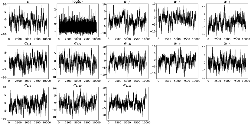
Figure 5: Trace plots for components of the parameter $\theta$ obtained using Metropolis under the prior $\theta\sim\mathcal{N}(-\mathbf{1},2I)$ with data $\mathcal{D}_{0}=\{(i/5,f^{*}(i/5))\}_{i=0}^{5}$ with $f^{*}$ as in Figure 10.

Sampling from $f\,|\,\mathcal{D}_{n-1}$:

In order to obtain a sample $\tilde{f}$ from the posterior marginal $f\,|\,\mathcal{D}_{n-1}$ we used ancestral sampling; i.e. we first sample $\tilde{\theta}$ from $\theta\,|\,\mathcal{D}_{n-1}$ and then we sample $\tilde{f}$ from $f\,|\,\mathcal{D}_{n-1},\tilde{\theta}$. To obtain the sample $\tilde{\theta}$ we used the aforementioned Metropolis algorithm.

Computing $\mathbb{E}[I(f)|\theta_{k},\tilde{\mathcal{D}}_{n}]$ and $\mathbb{V}[I(f)|\theta_{k},\tilde{\mathcal{D}}_{n}]$:

To compute $\mathbb{E}[I(f)|\theta_{k},\tilde{\mathcal{D}}_{n}]$ we used the $1d$ integration methodology discussed in Section D.2. In order to compute $\mathbb{V}[I(f)|\theta_{k},\tilde{\mathcal{D}}_{n}]$ we approximated the $2d$ integral in (8) with

$$\int_{0}^{1}\int_{0}^{1}k_{\theta_{k}}(x,y)\,\mathrm{d}x\,\mathrm{d}y\approx\frac{1}{N^{2}}\sum_{i=1}^{N}\sum_{j=1}^{N}k_{\theta_{k}}(x_{i},x_{j}),$$

where $x_{i}=\frac{i-1}{N-1}$ for some $N\in\mathbb{Z}^{+}$.

Returning $I(f)\,|\,\mathcal{D}_{n}$:

To compute $\mathbb{E}[I(f)\,|\,\mathcal{D}_{n}]$ we use the following approximation, by the law of total expectation,

$$\mathbb{E}[I(f)\,|\,\mathcal{D}_{n}] =\mathbb{E}[\mathbb{E}[I(f)\,|\,\mathcal{D}_{n},\theta]]$$

$$\approx\frac{1}{J}\sum_{i=1}^{J}\mathbb{E}[I(f)\,|\,\mathcal{D}_{n},\theta_{j}],$$

where $(\theta_{j})_{j=1}^{J}$ is sampled from Metropolis and the expectation is computed using the methodology in Section D.2. To compute $\mathbb{V}[I(f)\,|\,\mathcal{D}_{n}]$ we use the following approximation, again using the law of total variance,

$$\mathbb{V}[I(f)\,|\,\mathcal{D}_{n}] =\mathbb{E}[\mathbb{V}[I(f)\,|\,\mathcal{D}_{n},\theta]]+\mathbb{V}[\mathbb{E}[I(f)\,|\,\mathcal{D}_{n},\theta]]$$

$$\approx\frac{1}{J}\sum_{j=1}^{J}\mathbb{V}[I(f)\,|\,\mathcal{D}_{n},\theta_{j}]+s.v.\left(\{\mathbb{E}[I(f)\,|\,\mathcal{D}_{n},\theta_{j}]\}_{j=1}^{J}\right),$$

where $s.v.(X)$ is the sample variance of the set $X$. To compute the double integral in the computation of $\mathbb{V}[I(f)\,|\,\mathcal{D}_{n},\theta]$ we used the $2d$ integration methodology discussed in Section D.2.

D.4 Details Specific to E-AdapBC

It remains to be explained how the marginal likelihood $p(\mathcal{D}_{n-1}|\theta)$ was penalised to facilitate line 4 of Algorithm 2 describing the E-AdapBC method.

Line 4 of Algorithm 2 relates to computing the maximum of the (penalised) marginal likelihood $\theta\mapsto p(\mathcal{D}_{n-1}\,|\,\theta)-r(\theta)$. The likelihood function itself is derived from the Gaussian finite dimensional distribution of $f$ under the stochastic process model:

$$\log p(\mathcal{D}_{n-1}\,|\,\theta)=-\frac{n}{2}\log(2\pi)-\frac{1}{2}\log[\det(k_{\theta,X,X})]-\frac{[f_{X}^{*}-c\mathbf{1}]^{\top}k_{\theta,X,X}^{-1}[f_{X}^{*}-c\mathbf{1}]}{2},$$

where $X$ is the abscissae of $\mathcal{D}_{n-1}$ and $k_{\theta,X,X}$ is the matrix $k_{X,X}$ based on the kernel $k=k_{\theta}$.

It was demonstrated in Briol et al., (2019) that the empirical Bayesian approach to kernel parameters can lead to over-confident uncertainty quantification at small values of $n$ in the context of a standard BC method. The issue is more pronounced in E-AdapBC due to the increased dimension of the kernel parameter $\theta$ compared to StdBC. For this reason we included a penalty term $r(\theta)$ on line 2 to regularise the non-asymptotic regime (only) and to try to avoid over-confident estimation under the proposed E-AdapBC method. The regularisation term we used in $d$-dimensions was the following

$$r(\theta)=\prod_{i=1}^{d}\left(\lambda_{1}\|\ell_{\theta_{i}}(\cdot)\|_{1}+\lambda_{2}\|1/\ell_{\theta_{i}}(\cdot)\|_{1}\right)$$

where $\|g\|_{1}\vcentcolon=\int_{D}|g(x)|\mathrm{d}\pi(x)$. The specific form of regularisation was heuristically motivated (only) and many other choices are possible - to limit scope these were not explored. The regularisation term includes two parameters, $\lambda_{1}$ and $\lambda_{2}$, which are used respectively to ensure the length scale doesn’t get too large or small when the number $n$ of data is small. Specific values of $\lambda_{1}$ and $\lambda_{2}$ are reported in Appendix E. To optimise the (logarithm of the) penalised marginal likelihood the standard BFGS method was used.

Appendix E Details for the Experimental Assessment

In this section all remaining experiment-specific details are provided.

E.1 Illustration of Adaptation

In this section we detail the integration problem and how it was solved by AdapTrap, StdBC and E-AdapBC in the production of Figure 1.

The integrand in Figure 1 was randomly sampled according to the procedure in Section E.2 with parameters (to $3$ s.f.) $C=0.554,R=0.0726,H=1.64,F=2.65$ and $P=1$.

AdapTrap parameters:

For AdapTrap we used $\rho=0.5,m=5,k=2$ and with global error tolerances (from left to right) $\tau=0.06,0.04,0.02$.

StdBC setup:

In our StdBC arrangement we used the following Gaussian process model: Using the same Matérn ($\nu=3/2$) radial basis function as we used for E-AdapBC, we took $f\,|\,c,\sigma,\ell\sim\mathcal{GP}(c,k_{\sigma,\ell}(x,y))$, where

$$k_{\sigma,\ell}(x,y)=\sigma^{2}\phi_{\text{Mat}}^{\nu}\left(\frac{|x-y|}{\ell}\right).$$

In our implementation of StdBC we used the E-AdapBC algorithm with this stationary Gaussian process with $\theta=(c,\sigma,\ell)$, $r(\theta)=0$, with initial data $\mathcal{D}_{0}=\{(\frac{i}{10},f^{*}\left(\frac{i}{10}\right))\}_{i=0}^{10}$ and the point selection algorithm as detailed in Section D.1.

E-AdapBC setup:

In our E-AdapBC implementation we used the non-stationary model detailed in Appendix C, where $\ell_{1}$ is a piecewise linear function defined on $n=11$ uniform knots. Our regularisation term $r(\theta)$ was detailed in Section D.4, we took $\lambda_{1}=30$ and $\lambda_{2}=1$. We further used the initial data $\mathcal{D}_{0}=\{(\frac{i}{10},f^{*}\left(\frac{i}{10}\right))\}_{i=0}^{10}$ and the point selection algorithm as detailed in Section D.1.

E.2 Synthetic Assessment

In this section we detail how our results in Section 5.2 were created.

Synthetic Integrand Generation:

Our synthetic integrands in $d$ dimensions are generated as follows: First, we sample

1. $C=(C_{1},\ldots,C_{d})\sim U(0.1,0.9)^{d}$,

2. $R=(R_{1},\ldots,R_{d})\sim\text{Beta}(5,2)^{d}$,

3. $H=(H_{1},\ldots,H_{d})\sim U(0.5e,1.5e)^{d}$,

4. $F=(F_{1},\ldots,F_{d})\sim U(0,5)^{d}$,

5. $P=(P_{1},\ldots,P_{d})\sim\text{Bernoulli}(0.5)^{d}$.

Then we let

$$h(x)=\frac{1}{1+\exp\left(-80x\right)},\qquad g_{F}(x)=\begin{cases}0,&|x|<1,\\ \exp\left\{\frac{-1}{1-|x|^{2}}+\cos(F\pi|x|)\right\},&|x|\geq 1.\end{cases}$$

Our synthetic integrand is then

$$f^{*}(x)=\prod_{i=1}^{d}H_{i}g_{F_{i}}\left(\frac{1}{R_{i}}[x_{i}-C_{i}]\right)+(-1)^{P_{i}}[1/2-h(x_{i}-C_{i})],$$

with $x=(x_{1}\ldots,x_{d})$. In Figure 6 we plot $25$ randomly sampled synthetic integrands. To obtain the true integrals of these synthetic integrands we compute

$$\int_{[0,1]^{d}}f^{*}(x)\,\mathrm{d}x=\prod_{i=1}^{d}\int_{0}^{1}H_{i}g_{F_{i}}\left(\frac{1}{R_{i}}[x_{i}-C_{i}]\right)+(-1)^{P_{i}}[1/2-h(x_{i}-C_{i})]\,\mathrm{d}x_{i}$$

and for each of the $1d$ integration problems we integrate each term separately using the routine scipy.integrate.quad with its absolute error and relative error parameters taken as $10^{-10}$.

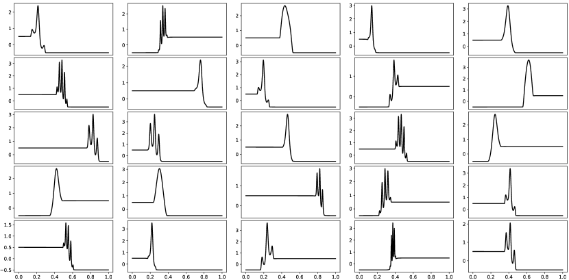
Figure 6: $25$ randomly generated synthetic functions in $1d$.

Experiments in $1d$:

For our experiments in $1d$ we sampled 100 integrands according to our synthetic integrand generation procedure discussed in the previous paragraph and used the same implementations of StdBC and E-AdapBC discussed in Section E.1.

Experiments in $3d$:

For our experiments in $3d$ we sampled 100 integrands according to our synthetic integrand generation procedure discussed in the previous paragraph. For both our implementations of StdBC and E-AdapBC we used the E-AdapBC algorithm with slight variations with each implementation. For both StdBC and E-AdapBC we took $\mathcal{D}_{0}=\{(x,f^{*}(x))\}_{x\in G}$ where $G=\{0,1/5,2/5,3/5,4/5,1\}^{3}$ and we used the point set selection algorithm discussed in Section D.1 with $U=\{i/40\}_{i=0}^{40}$ and $K_{1}=8000$.

For our implementation of E-AdapBC the underlying Gaussian process follows what we detailed in Appendix C and the regularisation term follows what was detailed in Section D.4 with $\lambda_{1}=9,\lambda_{2}=0.9$.

For our implementation of StdBC the underlying Gaussian process was $f\,|\,c,\sigma,\ell\sim\mathcal{GP}(c,k_{\sigma,\ell}(x,y))$ where,

$$k_{\sigma,\ell}(x,y)=\sigma^{2}\prod_{i=1}^{3}\phi_{\text{Mat}}^{\nu}\left(\frac{|x_{i}-y_{i}|}{\ell_{i}}\right).$$

where $\ell=(\ell_{1},\ell_{2},\ell_{3}),x=(x_{1},x_{2},x_{3}),y=(y_{1},y_{2},y_{3})$ and $\nu=3/2$. We further took $r(\theta)=2(|\ell_{1}|+|\ell_{2}|+|\ell_{3}|)$, where $\theta=(c,\sigma,\ell)$.

E.3 Variations of the Non-Stationary Model

In this section we explore variations in our non-stationary model specification in the use of the Algorithm 3.

Different Choice of Radial Basis Function:

As discussed in Appendix C the radial basis function $\phi$ was taken to be the standard Matérn radial basis function with smoothness parameter $\nu=3/2$ in all the experiments in the main text. In Figure 7 and Figure 9 we explore the robustness of E-AdapBC under different choices of radial basis function in our non-stationary model. In these experiments all other settings used in our non-stationary model (detailed in Appendix C) were kept the same. The radial basis functions that we chose were the Matérn radial basis function (17) with smoothness parameters $\nu=1/2,3/2,5/2$.

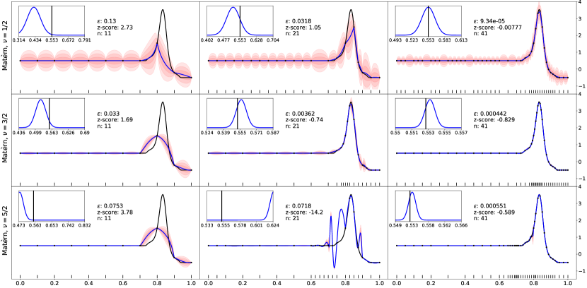
Figure 7: Each row corresponds to a different radial basis function with E-AdapBC run on the same integrand. The integrand was generated randomly from our synthetic integrand generation procedure with parameters (to 3 s.f.) $C=0.835,R=0.111,H=3.50,F=1.63,P=0.$ [Here represents the true integrand $f^{*}$, represents the mean of the conditional process $f|\mathcal{D}_{n}$ and represents pointwise credible intervals. The tick marks indicate where the integrand was evaluated. For each radial basis function the error $\epsilon\vcentcolon=|\mu_{n}(f^{*})-I(f^{*})|$, the z-score $[\mu_{n}(f^{*})-I(f^{*})]/\sigma_{n}(f^{*})$ and the number of integrand evaluations $n$ are reported. Inset panels compare the true value $I(f^{*})\approx 0.156$ to the distribution $I(f)|\mathcal{D}_{n}$.]

Different Lengthscale Fields:

In the following we explore the behaviour of E-AdapBC for different choices of lengthscale function in our non-stationary model. In these experiments all other settings used in our non-stationary model (detailed in Appendix C) were kept the same. The lengthscale functions that we compared were piecewise linear, piecewise constant

$$\ell_{\theta_{i}}^{\text{const.}}(x_{i})=\sum_{j=1}^{n}\beta_{i,j}\mathds{1}_{[(j-1)/n,j/n)}(x_{i}),$$

where $\mathds{1}_{A}(x)$ is the indicator function, and the exponential of piecewise linear

$$\ell_{\theta_{i}}^{\text{exp}}(x_{i})=\exp\left\{\sum_{j=1}^{n-1}\frac{\beta_{i,j+1}-\beta_{i,j}}{\bar{x}_{i,j+1}-\bar{x}_{i,j}}x_{i}-\frac{\beta_{i,j+1}-\beta_{i,j}}{\bar{x}_{i,j+1}-\bar{x}_{i,j}}\bar{x}_{i,j}+\beta_{i,j}\right\}.$$

For the piecewise constant lengthscale, to ensure positivity we took $\beta_{i,j}=\exp(\alpha_{i,j})$ and inferred the $\alpha_{i,j}\in\mathbb{R}$. For the piecewise constant lengthscale we took $n=10$ and for the other lengthscale functions we took $n=11$. See Figure 8 and Figure 9 for our results.

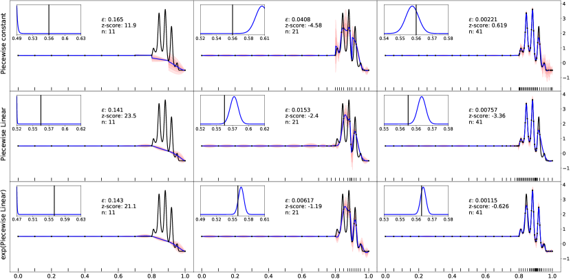
Figure 8: Each row corresponds to a different length scale function with E-AdapBC run on the same integrand. The integrand was generated randomly from our synthetic integrand generation procedure with parameters (to 3 s.f.) $C=0.882,R=0.0892,H=3.61,F=4.73,P=0.$ [Here represents the true integrand $f^{*}$, represents the mean of the conditional process $f|\mathcal{D}_{n}$ and represents pointwise credible intervals. The tick marks indicate where the integrand was evaluated. For each length scale function the error $\epsilon\vcentcolon=|\mu_{n}(f^{*})-I(f^{*})|$, the z-score $[\mu_{n}(f^{*})-I(f^{*})]/\sigma_{n}(f^{*})$ and the number of integrand evaluations $n$ are reported. Inset panels compare the true value $I(f^{*})\approx 0.156$ to the distribution $I(f)|\mathcal{D}_{n}$.]

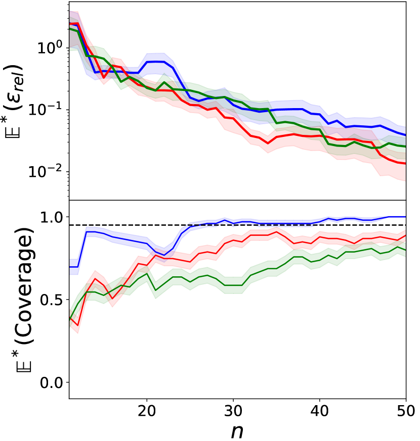
(a)

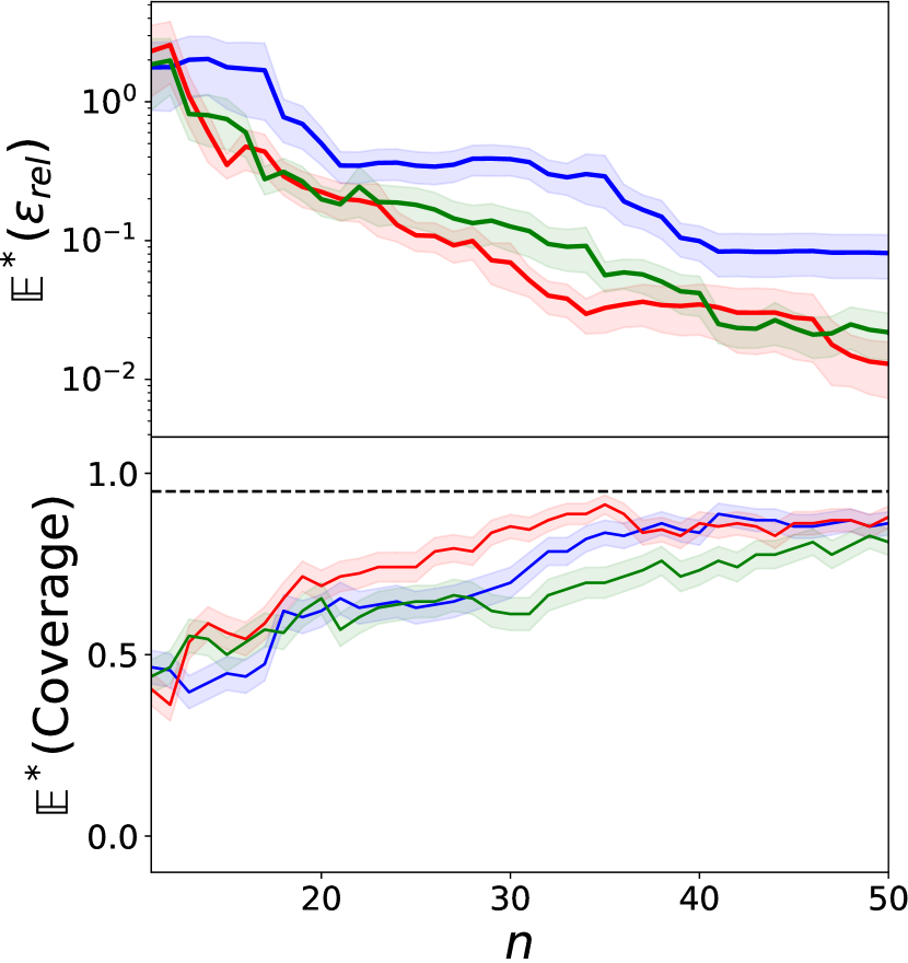
(b)

Figure 9: Synthetic assessment in $d=1$ of E-AdapBC with (a) different choices of radial basis function and (b) different choices of lengthscale function. Plot (a) Matérn $\nu=1/2$ ( ), Matérn $\nu=3/2$ ( ) and Matérn $\nu=5/2$ ( ), where 100 integrands were randomly generated. Plot (b) piecewise constant ( ), piecewise linear ( ) and exponential of piecewise linear ( ), where 100 integrands were randomly generated. Top row: the mean relative error against the number of evaluations $n$. Bottom row: the coverage frequencies for 95% credible intervals for each method. The notional coverage ( ) is indicated. [Standard errors displayed.]

E.4 Full Bayes vs Empirical Bayes

In the following we test the differences in behaviour between AdapBC (Algorithm 3) and E-AdapBC (Algorithm 2). For this test we ran both methods on the same integrand which was generated randomly from our synthetic integrand generation procedure detailed in Section E.2. Results are shown in Figure 10s.

For our implementation of E-AdapBC we used the same settings as detailed in Section E.1.

For our implementation of AdapBC we used the same initial data $\mathcal{D}_{0}=\{(\frac{i}{10},f^{*}\left(\frac{i}{10}\right))\}_{i=0}^{10}$, the same point set selection algorithm and the same non-stationary Gaussian process as our implementation of E-AdapBC used. Our choice of prior was $\theta\sim\mathcal{N}(-\mathbf{1},2I)$. When sampling the $\theta\,|\,\tilde{\mathcal{D}}_{n}$ and the $\theta\,|\,\mathcal{D}_{n-1}$, to ensure a tolerable acceptance rate in the output from Metropolis, at each step of AdapBC we set $s=0.3-0.07n$ for $n=0,\ldots,30$, so our proposal distribution used in Metropolis at step $n$ was $\mathcal{N}\left(\mathbf{0},(0.3-0.07n)^{2}I\right)$. In our approximation of $\mathbb{V}[I(f)\,|\,\theta_{k},\tilde{\mathcal{D}}_{n}]$ we set $N=101$. For our parameters $M$ and $K$ that control the number of samples of $f\,|\,\tilde{\mathcal{D}}_{n-1}$ and $\theta\,|\,\tilde{\mathcal{D}_{n}}$ in AdapBC respectively, we took $M=K=8$. All the output obtained from Metropolis was preceded by a length $1000$ burn in and was thinned by $5$. The $\theta_{0}$ in each run of Metropolis was taken as the last sample from the previous Metropolis output and at step $0$ was taken to be the mean of the prior on $\theta$. In outputting $I(f)\,|\,\mathcal{D}_{n}$ we took $J=50$.

Figure 10 suggests that AdapBC provides locally adaptive behaviour similar to E-AdapBC, but that AdapBC has better-calibrated uncertainty (in line with the previously documented over-confidence of Empirical Bayes in this context; Briol et al.,, 2019). However, the auxiliary computational cost associated with AdapBC is substantial - to produce Figure 10 the AdapBC method required 24 hours of CPU time whereas E-AdapBC required approximately one minute of CPU time. In addition, the need to carefully control the MCMC algorithm within AdapBC makes this method less attractive compared to E-AdapBC.

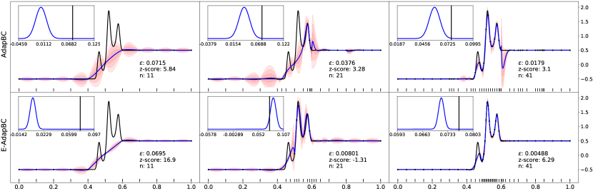
Figure 10: The upper and lower rows correspond to AdapBC and E-AdapBC respectively, run on the same integrand. The integrand was generated randomly from our synthetic integrand generation procedure with parameters (to 3 s.f.) $C=0.520,R=0.0897,H=1.87,F=3.04,P=1.$ [Here represents the true integrand $f^{*}$, represents the mean of the conditional process $f|\mathcal{D}_{n}$ and represents pointwise credible intervals. The tick marks indicate where the integrand was evaluated. For both methods the error $\epsilon\vcentcolon=|\mu_{n}(f^{*})-I(f^{*})|$, the z-score $[\mu_{n}(f^{*})-I(f^{*})]/\sigma_{n}(f^{*})$ and the number of integrand evaluations $n$ are reported. Inset panels compare the true value $I(f^{*})\approx 0.0764$ to the distribution $I(f)|\mathcal{D}_{n}$.]

E.5 Autonomous Robot Assessment

In this section we detail our autonomous robot experiment. The autonomous robot that we studied is due to Chrono, 2019b .

Details of Robot:

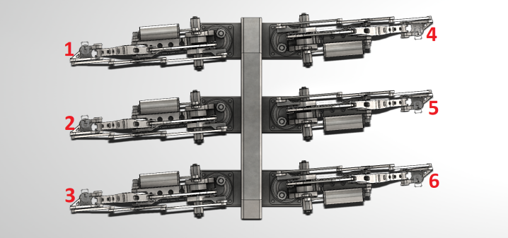
Figure 11: Elevated view of the robot, with each leg annotated.

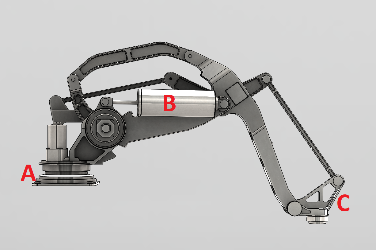
Figure 12: Detailed view of robot leg with each actuator labelled. Actuator A controls the rotation of the leg in the horizontal plane. Actuator B controls the up/down retraction of the leg. Actuator C controls the left/right extension of the leg.

In the following we provide the necessary details on the robot and how the actuators give motion. The robot was simulated in the open source physics engine Chrono, 2019a . The robot has $6$ legs with each leg consisting of $3$ actuators which control the walking motion of the robot; see Figure 11. Each leg has $3$ associated actuators that are depicted in Figure 12. Each actuator has a predefined loop. For each period $T=[\alpha,\beta]$ (lasting $\beta-\alpha=2$ seconds) of the loop the actuators are controlled as follows:

• Legs 1, 3 and 5:

  1. Actuator A:

     $$f_{A}(x)=0.2\sin\left(\pi(x-\alpha)\right).$$

  2. Actuator B:

     $$f_{B}(x)=\begin{cases}-0.2\,\text{Sig}(x-\alpha),&x\in[\alpha,\alpha+0.5],\\ -0.2,&x\in[\alpha+0.5,\alpha+1.5],\\ 0.2\,\text{Sig}(x-\alpha-1.5),&x\in[\alpha+1.5,\beta].\end{cases}$$

  3. Actuator C:

     $$f_{C}(x)=0.$$

• Legs 2, 4 and 6:

  1. Actuator A:

     $$g_{A}(x)=-0.2\sin\left(\pi(x-\alpha)\right)$$

  2. Actuator B:

     $$g_{B}(x)=\begin{cases}-0.2,&x\in[\alpha,\alpha+0.5],\\ 0.2\,\text{Sig}(x-\alpha-0.5),&x\in[\alpha+0.5,\alpha+1],\\ -0.2\,\text{Sig}(x-\alpha-1),&x\in[\alpha+1,\alpha+1.5],\\ -0.2,&x\in[\alpha+1.5,\beta].\end{cases}$$

  3. Actuator C:

     $$g_{C}(x)=0.$$

Here $\text{Sig}(x)$ is a polynomial smooth ramp such that $\text{Sig}(0)=0$ and $\text{Sig}(0.5)=1$.

Robot Experimental Details:

In our robot experiment we investigated the distribution of spatial location of the robot after a prescribed time of movement under uncertainty in the parameterisation of the functions that control the actuators in leg 1 of the robot. Our functions that controlled the actuators in leg 1 subject to our parameterisation are as follows, for each period $T=[\alpha,\beta]$:

$$f_{A}(x) =\sin(\pi(x-\alpha)),$$

$$f_{B}(x) =f_{B}(x)=\begin{cases}-(0.2+p_{1})\,\text{Sig}(x-\alpha),&x\in[\alpha,\alpha+(1-p_{2})/2],\\ -(0.2+p_{1}),&x\in[\alpha+(1-p_{2})/2,\alpha+(3+p_{2})/2],\\ (0.2+p_{1})\,\text{Sig}(x-\alpha-1.5),&x\in[\alpha+(3+p_{2})/2,\beta].\end{cases}$$

$$f_{C}(x) =p_{3},$$

Thus $p_{1}$ controls the how far the leg travels up and down in each period, $p_{2}$ controls how long the leg is down for in each period and $p_{3}$ controls the extension of the leg. In our experiment we took $(p_{1},p_{2},p_{3})\sim\mathcal{N}(0,\frac{1}{10}I_{3\times 3})$ and so after reparameterisation we have $x=(x_{1},x_{2},x_{3})\sim\mathcal{N}(0,I_{3\times 3})$ such that each $x_{i}=\frac{1}{\sqrt{10}}p_{i}$. In our experiment $z_{1}(x)$ and $z_{2}(x)$ were the spatial coordinates of the robot after $10$ seconds of movement. In our implementation we used Chrono’s inbuilt Barzila-Borwein solver with a discretisation time step of $0.005$s.

For both our implementations of StdBC and E-AdapBC we used the E-AdapBC algorithm with slight variations with each implementation. For both StdBC and E-AdapBC we took $\mathcal{D}_{0}=\{(x,f^{*}(x))\}_{x\in G}$ where $G=\{1/5,2/5,3/5,4/5\}^{3}$ and we used the point set selection algorithm discussed in Section D.1 with $U=\{i/40\}_{i=1}^{39}$ and $K_{1}=8000$. For each integrand we ran both methods to evaluate the integrand $200$ times and thus at termination we were using $264$ points.

For our implementation of E-AdapBC the underlying Gaussian process follows what we detailed in Appendix C and the regularisation term follows what was detailed in Section D.4 with $\lambda_{1}=10,\lambda_{2}=0.8$.

For our implementation of StdBC the underlying Gaussian process was $f\,|\,c,\sigma,\ell\sim\mathcal{GP}(c,k_{\sigma,\ell}(x,y))$ where,

$$k_{\sigma,\ell}(x,y)=\sigma^{2}\prod_{i=1}^{3}\phi_{\text{Mat}}^{\nu}\left(\frac{|x_{i}-y_{i}|}{\ell_{i}}\right).$$

where $\ell=(\ell_{1},\ell_{2},\ell_{3}),x=(x_{1},x_{2},x_{3}),y=(y_{1},y_{2},y_{3})$ and $\nu=3/2$. We further took $r(\theta)=2(|\ell_{1}|+|\ell_{2}|+|\ell_{3}|)$, where $\theta=(c,\sigma,\ell)$. The output of the experiments can be seen in Figure 13.

$f^{*}$	StdBC	E-AdapBC
$z_{1}$	$\mu_{n}=0.1095,\sigma_{n}=0.02129$	$\mu_{n}=0.06451,\sigma_{n}=0.008535$
$z_{2}$	$\mu_{n}=-5.760,\sigma_{n}=0.03812$	$\mu_{n}=-5.4913,\sigma_{n}=0.02373$
$z_{1}^{2}$	$\mu_{n}=0.1643,\sigma_{n}=0.01897$	$\mu_{n}=0.1252,\sigma_{n}=0.007559$
$z_{2}^{2}$	$\mu_{n}=32.93,\sigma_{n}=0.3969$	$\mu_{n}=32.43,\sigma_{n}=0.1562$

Figure 13: Autonomous robot experiment output to $4$ s.f.

Appendix F Full $k$-ary Trees

This section provides supporting material on the combinatorial results used in the average case analysis of the adaptive trapezoidal rule in Appendix A. In addition to basic definitions, it contains F.2 which was used in the proof of A.4.

Definition F.1 (Rooted tree).

A rooted tree is a (possibly infinite) tree where one node is specified to be the root.

The depth $d(v)$ of a node $v$ in a rooted tree is the length of the path from the root to $v$. A node $v$ is a child of a node $u$ if $u$ and $v$ are connected by an edge and the depth of $v$ is 1 greater than the depth of $u$. A leaf of a rooted tree is a node with degree 1. An inner node of a rooted tree is a node with degree greater than 1. The height of a rooted tree $T$ is $\sup_{v\in T}d(v).$

Definition F.2 ($k$-ary tree).

A $k$-ary tree is a rooted tree such that every node has at most $k$ children.

A full $k$-ary tree is a $k$-ary tree where every node has exactly $k$ children or $0$ children. We define the null tree to be a $k$-ary tree but not a full $k$-ary tree. Note that a tree with a single node is both a $k$-ary tree and a full $k$-ary tree. The set of all full $k$-ary trees is denoted $\mathcal{T}^{k}.$ One can always create a full $k$-ary tree from a $k$-ary tree:

Definition F.3 (Extension of a $k$-ary tree).

Let $S$ be a non-null $k$-ary tree. The extension of $S$ is the full $k$-ary tree $\overline{S}$ obtained by adding leaf nodes to $S$ such that every node in the original tree $S\subseteq\overline{S}$ has precisely $k$ children. The extension of the null $k$-ary tree is taken to be the single node full $k$-ary tree.

Note that this extension function $S\mapsto\overline{S}$ forms a bijection from the set of $k$-ary trees to the set of full $k$-ary trees.

Theorem F.1 (Full $k$-ary tree theorem).

Let $S$ be a $k$-ary tree with $n$ nodes and let $\overline{S}$ be its extension. Then $\overline{S}$ has $nk+1$ nodes.

Proof.

The proof is by induction. The base case is trivial: Consider the null tree with $0$ nodes, the extension of this tree has $1$ node. Assume now that every $k$-ary tree with $n$ nodes has, in its extension, $nk+1$ nodes. Note that any $k$-ary tree with $n+1$ nodes can be formed by adding an additional node and edge to a $k$-ary tree with $n$ nodes. We can only add this extra node and edge to a node of degree at most $k$. In any of these cases the number of extra nodes added in this new tree’s extension is $k$. That is, in this new tree of $n+1$ nodes, the number of nodes in its extension is $nk+1+k=(n+1)k+1$. ∎

Thus a full $k$-ary tree with $n$ nodes has $\frac{n-1}{k}$ inner nodes and $\frac{(k-1)n+1}{k}$ leaves.

Next we consider the problem of counting the number of $k$-ary trees with a given number of nodes. Let $C_{n}^{(k)}$ be the number of $k$-ary trees with $n$ nodes with corresponding generating function $C_{k}(x)\coloneqq\sum_{i=0}^{\infty}C_{i}^{(k)}x^{i}.$ From (Graham et al.,, 1994), the $C_{n}^{(k)}$ follow the recurrence relation

$$C^{(k)}_{n+1}=\sum_{n_{1}+n_{2}+\ldots+n_{k}=n}C^{(k)}_{n_{1}}C^{(k)}_{n_{2}}\ldots C^{(k)}_{n_{k}}.$$

This recurrence relation yields the following functional equation,

$$C_{k}(x)=1+x[C_{k}(x)]^{k}.$$

For $k=2$ this has the solution

$$C_{2}(x)=\frac{1-\sqrt{1-4x}}{2x}.$$ (18)

Theorem F.2 (Number of $k$-ary trees with $n$ nodes).

The total number of $k$-ary trees with $n$ nodes is

$$C_{n}^{(k)}=\frac{1}{(k-1)n+1}\binom{nk}{n},$$

where $C_{n}^{(k)}$ is the $n$th $k$-Catalan number. Note that for $k=2$, we get the standard Catalan numbers.

Proof.

Use the Lagrange inversion theorem on the generating function’s functional equation. See (Graham et al.,, 1994). ∎

Since the extension function defines a bijection from the set of $k$-ary trees to the set of full $k$-ary trees, the above result also counts the total number of full $k$-ary trees with $nk+1$ nodes as $C_{n}^{(k)}.$

Definition F.4 (Preorder traversal).

Let $T\in\mathcal{T}^{k}$ be finite. A preorder traversal of $T$ is a sequence of nodes $\langle v_{i}\rangle_{i=1}^{N}$ that is defined by the following steps:

1. Visit the root.

2. For $i=1,\ldots,k$, traverse the $i$th subtree from the left.

For example, consider the following full $3$-ary tree:

The preorder traversal of this tree is the sequence $(1,0),(1,1),(2,1),(3,1),(7,2),(19,3)$, $(20,3),(21,3),(8,2),(9,2)$.

References

- Ba et al., (2012) Ba, S., Joseph, V. R., et al. (2012). Composite Gaussian process models for emulating expensive functions. The Annals of Applied Statistics, 6(4):1838–1860.
- Berntsen et al., (1991) Berntsen, J., Espelid, T. O., and Sørevik, T. (1991). On the subdivision strategy in adaptive quadrature algorithms. Journal of Computational and Applied Mathematics, 35(1-3):119–132.
- Bogachev, (1998) Bogachev, V. I. (1998). Gaussian Measures. Number 62 in Mathematical Surveys and Monographs. American Mathematical Society.
- Briol et al., (2019) Briol, F.-X., Oates, C. J., Girolami, M., Osborne, M. A., and Sejdinovic, D. (2019). Probabilistic Integration: A Role in Statistical Computation? Statistical Science, 34(1):1–22. Appeared with discussion and rejoinder.
- Chai and Garnett, (2019) Chai, H. and Garnett, R. (2019). Improving Quadrature for Constrained Integrands. In Proceedings of the 22nd International Conference on Artificial Intelligence and Statistics.
- Chaloner and Verdinelli, (1995) Chaloner, K. and Verdinelli, I. (1995). Bayesian experimental design: A review. Statistical Science, 10(3):273–304.
- Chkrebtii and Campbell, (2019) Chkrebtii, O. and Campbell, D. (2019). Adaptive step-size selection for state-space probabilistic differential equation solvers. Statistics and Computing. To appear.
- (8) Chrono, P. (2019a). Chrono: An Open Source Framework for the Physics-Based Simulation of Dynamic Systems. Accessed: 2019-09-15.
- (9) Chrono, P. (2019b). Make a spider robot in solidworks and simulate it. Accessed: 2019-10-6.
- Clancy et al., (2014) Clancy, N., Ding, Y., Hamilton, C., Hickernell, F. J., and Zhang, Y. (2014). The cost of deterministic, adaptive, automatic algorithms: Cones, not balls. Journal of Complexity, 30(1):21–45.
- Damian et al., (2001) Damian, D., Sampson, P. D., and Guttorp, P. (2001). Bayesian estimation of semi-parametric non-stationary spatial covariance structures. Environmetrics, 12(2):161–178.
- Damianou and Lawrence, (2013) Damianou, A. and Lawrence, N. (2013). Deep Gaussian processes. In Artificial Intelligence and Statistics, pages 207–215.
- Davis and Rabinowitz, (1984) Davis, P. J. and Rabinowitz, P. (1984). Methods of Numerical Integration. Academic Press.
- Diaconis, (1988) Diaconis, P. (1988). Bayesian numerical analysis. Statistical Decision Theory and Related Topics IV, 1:163–175.
- Dick and Pillichshammer, (2010) Dick, J. and Pillichshammer, F. (2010). Digital nets and sequences: discrepancy theory and quasi–Monte Carlo integration. Cambridge University Press.
- Dunlop et al., (2018) Dunlop, M., Girolami, M., Stuart, A., and Teckentrup, A. (2018). How Deep Are Deep Gaussian Processes? Journal of Machine Learning Research, 19(1):2100–2145.
- Gonnet, (2012) Gonnet, P. (2012). A Review of Error Estimation in Adaptive Quadrature. ACM Computing Surveys (CSUR), 44(4):22.
- Graham et al., (1994) Graham, R. L., Knuth, D. E., and Patashnik, O. (1994). Concrete Mathematics: A Foundation for Computer Science. Addison-Wesley Longman Publishing Co., Inc., Boston, MA, USA, 2nd edition.
- Gramacy and Lee, (2008) Gramacy, R. B. and Lee, H. K. H. (2008). Bayesian Treed Gaussian Process Models with an Application to Computer Modeling. Journal of the American Statistical Association, 103(483):1119–1130.
- Gunter et al., (2014) Gunter, T., Osborne, M. A., Garnett, R., Hennig, P., and Roberts, S. J. (2014). Sampling for Inference in Probabilistic Models with Fast Bayesian Quadrature. In Advances in Neural Information Processing Systems, pages 2789–2797.
- Hennig et al., (2015) Hennig, P., Osborne, M. A., and Girolami, M. (2015). Probabilistic numerics and uncertainty in computations. Proceedings of the Royal Society A: Mathematical, Physical and Engineering Sciences, 471(2179):20150142.
- Higdon et al., (1999) Higdon, D. M., Swall, J. L., and Kern, J. C. (1999). Bayesian Statistics, volume 6, chapter Non-Stationary Spatial Modeling.
- Jagadeeswaran and Hickernell, (2019) Jagadeeswaran, R. and Hickernell, F. J. (2019). Fast Automatic Bayesian Cubature Using Lattice Sampling. Statistics and Computing. To appear.
- Jiang et al., (2019) Jiang, S., Chai, H., Gonzalez, J., and Garnett, R. (2019). Efficient nonmyopic Bayesian optimization and quadrature. arXiv:1909.04568.
- Kahaner and Rechard, (1987) Kahaner, D. K. and Rechard, O. W. (1987). TWODQD an adaptive routine for two-dimensional integration. Journal of Computational and Applied Mathematics, 17(1-2):215–234.
- Kanagawa and Hennig, (2019) Kanagawa, M. and Hennig, P. (2019). Convergence Guarantees for Adaptive Bayesian Quadrature Methods. arXiv:1905.10271.
- Karvonen et al., (2018) Karvonen, T., Oates, C. J., and Särkkä, S. (2018). A Bayes–Sard cubature method. In 32nd Conference on Neural Information Processing Systems (NeurIPS 2018).
- Karvonen and Särkkä, (2018) Karvonen, T. and Särkkä, S. (2018). Fully Symmetric Kernel Quadrature. SIAM Journal on Scientific Computing, 40(2):A697–A720.
- Karvonen et al., (2019) Karvonen, T., Särkkä, S., and Oates, C. J. (2019). Symmetry Exploits for Bayesian Cubature Methods. Statistics and Computing. To appear.
- Kim et al., (2005) Kim, H.-M., Mallick, B. K., and Holmes, C. C. (2005). Analyzing Nonstationary Spatial Data Using Piecewise Gaussian Processes. Journal of the American Statistical Association, 100(470):653–668.
- Larkin, (1972) Larkin, F. (1972). Gaussian measure in Hilbert space and applications in numerical analysis. Rocky Mountain Journal of Mathematics, 2(3):379–422.
- Larkin, (1974) Larkin, F. (1974). Probabilistic error estimates in spline interpolation and quadrature. In IFIP Congress; Information Processing, volume 74, pages 605–609.
- Minka, (2000) Minka, T. (2000). Deriving Quadrature Rules from Gaussian Processes. Technical report, Statistics Department, Carnegie Mellon University.
- Oettershagen, (2017) Oettershagen, J. (2017). Construction of Optimal Cubature Algorithms with Applications to Econometrics and Uncertainty Quantification. PhD thesis, Institut für Numerische Simulation, Universität Bonn.
- O’Hagan, (1991) O’Hagan, A. (1991). Bayes–Hermite quadrature. Journal of Statistical Planning and Inference, 29(3):245–260.
- Osborne, (2010) Osborne, M. (2010). Bayesian Gaussian Processes for Sequential Prediction, Optimisation and Quadrature. PhD thesis, University of Oxford.
- Osborne et al., (2012) Osborne, M. A., Duvenaud, D., Garnett, R., Rasmussen, C. E., Roberts, S. J., and Ghahramani, Z. (2012). Active Learning of Model Evidence Using Bayesian Quadrature. In Advances in Neural Information Processing Systems.
- Overstall et al., (2018) Overstall, A. M., McGree, J. M., and Drovandi, C. C. (2018). An approach for finding fully Bayesian optimal designs using normal-based approximations to loss functions. Statistics and Computing, 28(2):343–358.
- Paciorek, (2003) Paciorek, C. J. (2003). Nonstationary Gaussian processes for regression and spatial modelling. PhD thesis, Carnegie Mellon University.
- Piessens, (1983) Piessens, R. (1983). Quadpack : a subroutine package for automatic integration. Springer-Verlag.
- Pronzato and Zhigljavsky, (2018) Pronzato, L. and Zhigljavsky, A. (2018). Bayesian quadrature and energy minimization for space-filling design. arXiv:1808.10722.
- Prüher et al., (2018) Prüher, J., Karvonen, T., Oates, C. J., Straka, O., and Särkkä, S. (2018). Improved calibration of numerical integration error in sigma-point filters. arXiv:1811.11474.
- Rabe-Hesketh et al., (2002) Rabe-Hesketh, S., Skrondal, A., and Pickles, A. (2002). Reliable estimation of generalized linear mixed models using adaptive quadrature. The Stata Journal, 2(1):1–21.
- Rasmussen and Williams, (2006) Rasmussen, C. E. and Williams, C. K. I. (2006). Gaussian Processes for Machine Learning. MIT Press.
- Richardson and Gaunt, (1927) Richardson, L. F. and Gaunt, J. A. (1927). The deferred approach to the limit. Philosophical Transactions of the Royal Society of London. Series A, 226(636-646):299–361.
- Ritter, (2000) Ritter, K. (2000). Average-Case Analysis of Numerical Problems, volume 1733 of Lecture Notes in Mathematics. Springer Berlin Heidelberg, Berlin, Heidelberg.
- Roininen et al., (2019) Roininen, L., Girolami, M., Lasanen, S., and Markkanen, M. (2019). Hyperpriors for Matérn fields with applications in Bayesian inversion. Inverse Problems & Imaging, 13(1):1–29.
- Sampson and Guttorp, (1992) Sampson, P. and Guttorp, P. (1992). Nonparametric Estimation of Nonstationary Spatial Covariance Structure. Journal of the American Statistical Association, 87(417):108–119.
- Santin et al., (2017) Santin, G., Haasdonk Communicated by De Rossi, B. A., and Francomano, E. (2017). Convergence rate of the data-independent P-greedy algorithm in kernel-based approximation. Dolomites Research Notes on Approximation, 10.
- Schmidt and O’Hagan, (2003) Schmidt, A. M. and O’Hagan, A. (2003). Bayesian Inference for Non-Stationary Spatial Covariance Structure via Spatial Deformations. Journal of the Royal Statistical Society, Series B, 65(3):743–758.
- Sul’din, (1959) Sul’din, A. V. (1959). Wiener measure and its applications to approximation methods. I. Izv. Vyssh. Uchebn. Zaved. Mat., 6(13):145–158.
- Sul’din, (1960) Sul’din, A. V. (1960). Wiener measure and its applications to approximation methods. II. Izv. Vyssh. Uchebn. Zaved. Mat., 5(18):165–179.