Repeated Gravitational Lensing of Gravitational Waves in Hierarchical Black Hole Triples

Abstract

We consider binary black holes (BBHs) in a hierarchical triple system where a more compact, less-massive binary is emitting detectable gravitational waves (GWs), and the tertiary is a supermassive BH at the center of a nuclear star cluster. As previous works have shown, the orbital motion of the outer binary can generate a detectable relativistic Doppler boost of the GWs emitted by the orbiting inner binary. We show here that for outer-binary orbits with a period of order one year, there can be a non-negligible probability for repeated gravitational lensing of the GWs emitted by the inner binary. Repeating gravitational lensing events could be detected by the LISA observatory as periodic GW amplitude spikes before the BBH enters the LIGO band. Such a detection would confirm the origin of some BBH mergers in nuclear star clusters. GW lensing also offers new testing grounds for strong gravity.

I Introduction

Although gravitational waves (GWs) from merging binary black holes (BBHs) have been detected (The LIGO Scientific Collaboration et al., 2018), the astrophysical origin and path towards merger of these systems remains a mystery. GWs emitted during inspiral and merger encode the binary parameters: masses, mass ratios, eccentricities, and spins. A major goal of the GW-astrophysics community is to use the measured distributions of these parameters to infer their astrophysical origins (e.g., Ref. The LIGO Scientific Collaboration and the Virgo Collaboration, 2018).

For this task, binary parameters are not the only useful information that GWs can provide. GWs can also carry information on the merger environment. This can occur either through external actors affecting the GW inspiral, such as gas dynamics slowing or accelerating the inspiral (Yunes et al., 2011; Kocsis et al., 2011; Fedrow et al., 2017; D’Orazio and Loeb, 2018; Derdzinski et al., 2019), or tidal effects in non-BBH inspiral (see Ref. LIGO Scientific Collaboration and the Virgo Collaboration, 2018, and references therin). The environment of the merger can also affect the observed waveform without directly affecting the inspiral. Such a situation arises through frame-dependent effects caused by relative motion of the GW source or an intervening gravitational potential resulting in relativistic Doppler boosting and gravitational lensing of the rest-frame GWs, as well as time-dependent gravitational redshift and the Shapiro-delay (Meiron et al., 2017). In this work we consider such frame-dependent modulations, focusing on gravitational lensing of GWs.

Previous papers have considered Doppler boost and gravitational lensing of GWs. The Doppler boost due to peculiar velocities of GW sources has been investigated for its degeneracy with the source luminosity distance (e.g., Ref. Kocsis et al., 2006; Bonvin et al., 2017; Chen et al., 2019). Recent work has also considered the Doppler boost of GWs, detectable in deviations from the vacuum GW phase, as an indicator of orbital motion around a companion BH (Inayoshi et al., 2017; Meiron et al., 2017; Robson et al., 2018; Wong et al., 2019) or other intervening mass distributions (Randall and Xianyu, 2019).

Lensing of GWs has been considered in the wave and geometrical optics limits (e.g., Ref. Takahashi and Nakamura, 2003). The lens itself has been imagined as an intervening mass at a large distance from the observer and from the source (e.g., Refs. Ruffa, 1999; Takahashi and Nakamura, 2003; Christian et al., 2018), but also as a supermassive BH (SMBH) that an inspiraling BBH orbits in an hierarchical triple (Kocsis, 2013). The latter case, most relevant to this study, considers observables in the magnified GW echoes caused by lensing-induced time delays; these calculations were carried out for a source that is stationary with respect to the SMBH lens.

Here we consider for the first time a different lensing regime, the case of a moving lensed source of GWs. Importantly, we find that such a system can have orders of magnitude higher probabilities for lensing, exhibit a unique, and possibly repeating magnification signature in the GW amplitude, and naturally arise in BBH formation scenarios that involve hierarchical triple systems with a SMBH tertiary, e.g., Kozai-Lidov oscillation-induced mergers (Antonini and Perets, 2012), binary-EMRI capture (Chen and Han, 2018; Chen et al., 2019; Fernández and Kobayashi, 2018), and, generally, the formation of binaries in the disks of Active Galactic Nuclei (AGN) (Bellovary et al., 2016; Stone et al., 2017; Bartos et al., 2017; McKernan et al., 2018).

We estimate that BBH inspirals and mergers that occur while a BBH is on a year-timescale orbit around a tertiary SMBH could be detected by the Laser Interferometer Space Antenna (LISA, Amaro-Seoane and et al., 2017) as exhibiting strong (factor of $\sim 1.5$) periodic magnification of the GW amplitude. Depending on astrophysical formation channels, up to of order one percent of all such BBHs passing through the LISA band could exhibit repeated lensing. Detection of GW lensing would strongly constrain the distribution of BBHs in galactic nuclei and offer tests of gravity through GW propagation (Chesler and Loeb, 2017). Non-detection will help rule out some formation scenarios.

This work is organized as follows. In §II we present the probability, timescale, and magnification of GW lensing events in a general wave-optics treatment, and for a wide range of triple-system parameters. In §III we illustrate the GW amplitude evolution for two example lensed systems. In §IV we consider the astrophysical population of such triple systems in order to gauge the detection probability of a lensed event. In §V we discuss implications for understanding astrophysical formation channels of BBH mergers as well as studying gravity. In §VI we summarize our main conclusions.

II Lensing Regimes

We begin by specifying the different lensing regimes for hierarchical triples and the probability for detecting lensing events in these regimes. Throughout we consider a smaller (in separation and mass) inner BBH, called binary $i$ with observed total mass $M_{i}$, orbital frequency $f_{i}$, and mass ratio $q_{i}$. This binary orbits a larger black hole with mass $M_{L}$ in an outer binary called binary $o$ with total mass, orbital frequency, and mass ratio, $M_{o}$, $f_{o}$, $q_{o}$. The chirp mass is given in terms of the binary total mass as $\mathcal{M}=Mq^{3/5}/(1+q)^{6/5}$, where $q\leq 1$ is the ratio of the two binary masses. For a generally eccentric orbit, GWs are emitted by the inner binary at $n^{\text{th}}$ harmonics of the orbital frequency $f_{\text{GW},i}\equiv nf_{i}$. Throughout we primarily consider binaries on circular orbits where $n=2$. As the BBH passes behind the tertiary SMBH along the observer’s line of sight, the emitted GWs are lensed. We primarily consider the case where $M_{L}$ is a larger, SMBH tertiary and the inner binary is one that will eventually merge in the LIGO band. In all cases we consider only stable hierarchical triples. We gauge stability with the criteria of Ref. Mardling and Aarseth (2001),

$$f_{i} \geq q^{1/2}_{o}Y^{-3/2}f_{o}\quad$$ (1)

$$Y \equiv 3.3\left[\frac{2}{3}\left(\frac{1+q_{o}}{q_{o}}\right)\right]^{2/5}\left(1-0.3\frac{i}{\pi}\right)$$

where we conservatively assume that the relative inclination $i$ of inner and outer binary angular momentum is set to $\pi$ radians.

II.1 Spatial Scales: Wave vs. Geometrical Optics

Because of the relatively long wavelength of GWs compared to electromagnetic waves, the wave period can be comparable to the lensing time delay, in which case we must treat lensing in the wave-optics regime (Schneider et al., 1992). The wave- and geometrical optics regimes are delineated by comparing the time delay and the GW period via the parameter (e.g., Ref. Takahashi and Nakamura, 2003),

$$\chi\equiv\frac{8\pi GM_{L}}{c^{3}}f_{\text{GW},i},$$ (2)

where $M_{L}$ and $f_{\text{GW},i}$ are the observer-frame (redshifted) quantities. The inner-binary GW frequency $f_{\text{GW},i}$ is set by the inner-binary orbital period and eccentricity. In the limit that $\chi\gg 1$, the wave-optics treatment asymptotes to the geometrical optics case.

While not wholly in the geometrical optics regime, for $\chi\geq 1$ lensing magnification becomes significant. Hence, it is useful to rearrange the above equation for the frequency above which the transition to geometrical optics begins and significant magnification is expected,

$$f_{\text{GW},i}\geq 0.08\text{Hz}\left(\frac{M_{L}}{10^{5}{M_{\odot}}}\right)^{-1}.$$ (3)

This means that for GW emitting BBHs orbiting SMBH lenses with masses above $10^{5}{M_{\odot}}$, the transition from wave-optics to geometrical optics begins before or during the evolution of the BBH through the LISA band ($\sim 10^{-3}$ Hz to $10^{-1}$ Hz for the context of this work).

II.2 Timescales

We further delineate three different lensing regimes based upon the motion of the source with respect to the lens over its observable lifetime. The three relevant timescales are the orbital period of the outer binary $1/f_{o}$, the time in band, $\tau_{\text{obs}}$, and the time for the inner-binary GW source to cross the Einstein radius of the lens, $\tau_{\text{lens}}$. The resulting three lensing regimes are

• The Repeating-Lens Regime: $1/f_{o}\lesssim\tau_{\text{obs}}$

• The Slowly-Moving Lens Regime: $1/f_{o}\geq\tau_{\text{obs}}\geq\tau_{\text{lens}}$

• The Stationary-Lens Regime: $1/f_{o}\geq\tau_{\text{obs}}\leq\tau_{\text{lens}}$.

The time in band $\tau_{\text{obs}}$ is set by the time that the inner binary emits GWs above a set signal-to-noise ratio (SNR) in all GW-bands through which the binary passes over its lifetime, and $\tau_{\text{lens}}\equiv r^{\text{max}}_{E}/v_{\text{orb},o}$, where $v_{\text{orb},o}$ is the orbital velocity of the inner binary around the tertiary SMBH, and $r^{\text{max}}_{E}=\sqrt{4GM_{L}/c^{2}a_{o}\sin{I_{o}}}$ is the Einstein radius when the inner binary (source) is directly behind the tertiary (lens), for outer binary inclination $I_{o}$ (see e.g., Ref. D’Orazio and Di Stefano, 2018).

In the repeating-lens regime we require, as a hard limit on detection of such a flare, that the timescale constraint $\tau_{\text{lens}}\gg f^{-1}_{\text{GW},i}$ be satisfied. We find this only to affect very short outer-orbital periods for small tertiary masses, which we have already shown exhibit low magnification and, as we show in the subsequent sections are low probability events due to rapid decay of the inner binary into the tertiary SMBH.

II.3 Probabilities

The probability for the tertiary SMBH to lens GWs emitted by the inner binary can be computed separately in each of the above-mentioned regimes. Conservatively, we focus on the geometrical optics limit. In the wave-optics limits, these probabilities are higher (Ruffa, 1999), but as we discuss below, the magnification can be lower in that case, and not as observationally interesting. Hence, we compute the probability of a significant lensing event in the geometrical optics limit as in Refs. D’Orazio and Di Stefano (2018, 2019). To do so we define a significant lensing event as one in which the projected distance between the GW source and the SMBH lens falls within one Einstein radius (see $r^{\text{max}}_{E}$ above). The lensing probability is then computed from the geometrical cross section of the Einstein radius compared to the total area available to the inner binary along its orbit around the tertiary, $M_{L}$:

1. In the repeating-lens regime we observe the system for longer than an orbit of the outer binary and so treat the outer orbit as a ring that can be randomly oriented with respect to the line of sight. Then the probability that this ring falls within one Einstein radius of the lens is the lensing probability in the repeating-lens regime,

   $$\mathcal{P}_{\text{rl}} \approx \frac{2}{\pi}\sin^{-1}\left(\frac{r^{\text{max}}_{E}}{a}\right)$$

   $$= \frac{2}{\pi}\sin^{-1}\left[\sqrt{\frac{4GM_{L}}{c^{2}}}\frac{\left(2\pi f_{o}\right)^{1/3}}{\left[GM_{o}\right]^{1/6}}\right].$$

   This is the probability that the source, observed for one orbit, will be inclined within one Einstein radius of the lens. This condition sets the required outer-binary inclination given the outer-binary separation and the lens mass (see Eq. (6) of Ref. D’Orazio and Di Stefano, 2018). The duration of strongly lensed emission in this regime is given approximately by $0.5\mathcal{P}_{rl}P_{o}$.

2. In the slowly-moving regime, the outer binary does not execute a full orbit while GWs from the inner binary are detectable, and the above probability is simply decreased by the fraction of an outer orbit that is observed.

   $$\mathcal{P}_{\text{sm}}\approx\text{min}\left\{\frac{\tau_{\text{obs}}f_{o}}{2},1\right\}\mathcal{P}_{rl}.$$ (5)

3. In the stationary-lens regime the probability decreases to the ratio of the area enclosed by the Einstein radius to the sphere of possible positions of the inner binary on its orbit at an arbitrary inclination around the lens,

   $$\mathcal{P}_{\text{sl}} \approx \frac{GM_{L}}{a_{o}c^{2}}=\dfrac{\dfrac{GM_{L}}{c^{3}}2\pi f_{o}}{\left(\dfrac{GM_{o}}{c^{3}}2\pi f_{o}\right)^{1/3}}$$ (6)

   $$\approx \left(\frac{GM_{o}}{c^{3}}2\pi f_{o}\right)^{2/3}.$$

We label the general probability of a lensing event, encompassing all of the above lensing regimes, $\mathcal{P}$.

Figure 1: Contours of the lensing probability $\mathcal{P}$ delineated into the three lensing regimes discussed in the text (marked by the solid white lines). The vertical axis denotes the orbital frequency of the outer binary and the horizontal axis denotes the mass of the tertiary BH that the inspiraling BBH orbits. The cyan dashed lines pick out specific lensing-probability contours. The black region denotes unphysical outer orbits set by the innermost stable circular orbit (ISCO) and the gray region denotes unstable hierarchical triples (assuming the inner binary is separated such that it will merge in a Hubble time). Above the bright green line, the outer binary inspirals in less than a Hubble time, and hence, as discussed in §IV, such systems may be less common. Triple systems falling above the magenta line will have lensing durations that are shorter than than 100 seconds, and are, hence, not detectable at the ($\sim 10^{-2}$ Hz) GW frequency band of interest.

Figure 1 shows contours of these lensing probabilities for a range of relevant outer binary frequencies (vertical axis) and lens masses (horizontal axis). Here purple contours denote low probabilities while yellow contours denote high probabilities, with the labeled dashed-cyan lines delineating $1\%$, $10\%$, and $50\%$ probabilities. These probabilities are computed assuming that the emitting BBH falls within one Einstein radius of the lens in projection, for randomly oriented outer orbits. The black and gray regions shade forbidden orbits due to the innermost stable circular orbit (ISCO) of the outer binary, and triple stability (Eq. 1), respectively.

The white labeled lines are drawn to delineate the three different timescale regimes discussed above. It is apparent that the highest probabilities for lensing occur for short outer orbits, in the repeating-lens regime, while chance lensing of BBHs on longer period orbits are rare. As we will discuss in the next section, however, shorter outer orbits may be depleted by rapid orbital decay into the central SMBH. In green we have drawn a line where the GW-induced inspiral time of the BBH into the SMBH is equal to the Hubble time, for a circular outer orbit. Systems falling above this green line are less likely to last long enough to fulfill their full lensing probability. The magenta line denotes systems above which the lensing timescale is shorter than the period of a GW at $10^{-2}$ Hz. The majority of triple parameter space allows lensing flares that are long enough in duration for detection in the LISA band.

To draw Figure 1, we have chosen an inner-binary with equal mass components, a total mass of $50{M_{\odot}}$, and a separation such that it will merge in a Hubble time. We choose an observation time of $8$ yrs corresponding to a maximum observation time in the LISA band (e.g., Ref. Sesana, 2016). For longer (shorter) observation times, the white lines delineating the different lensing regimes shift downwards (upwards). Hence, this plot is qualitatively similar for year timescale observations that would apply to BBH inspirals that leave the LISA band during the LISA mission, or for those observed in a 4-year mission. For the heavy stellar-mass BBHs that can be observed for year timescales with LISA, the most promising lensing systems are those with a $\sim 0.1-8$ year outer-orbital period and a central SMBH with mass in the range of $10^{5}{M_{\odot}}-10^{10}{M_{\odot}}$. As discussed above, the lensing magnification will be low in the LISA band for SMBH lenses below $10^{5}{M_{\odot}}$.

II.4 Magnification

In the case of a point mass lens, the GW-amplitude magnification factor due to lensing can be written in terms of the parameter $\chi$ (Takahashi and Nakamura, 2003), defined in Eq. (2),

$$F(\chi) = \exp\left\{\frac{\pi^{2}\chi}{2}+\sqrt{-1}\pi\chi\left[\log\left(\pi\chi\right)-2\phi_{m}(u)\right]\right\}\Gamma\left(1-\sqrt{-1}\pi\chi\right)\ {}_{1}F_{1}\left(\sqrt{-1}\pi\chi,1;\sqrt{-1}\pi\chi u^{2}\right)$$ (7)

$$\phi_{m}(u) \equiv \left(x_{m}-u\right)^{2}/2-\log x_{m},\qquad x_{m}=\frac{u+\sqrt{u^{2}+4}}{2}$$

where $u$ is the separation between source and lens in units of the Einstein radius, $r_{E}=\sqrt{4GM_{L}/c^{2}a_{o}\sin{I_{o}}\sin\left(2\pi/P_{o}t\right)}$, assuming a circular orbit here and for outer binary inclination $I_{o}$ (see e.g., Ref. D’Orazio and Di Stefano, 2018), and ${}_{1}F_{1}$ is the confluent hypergeometric function of the first kind.

For $\chi\ll 1$ the GWs are diffracted by the BH, resulting in very little magnification. As $\chi$ approaches unity, however, GWs traversing the lens BH, being coherent, interfere resulting in a time-oscillatory magnification with amplitude approaching that of the point mass geometrical optics limit ($|\mu_{+}|+|\mu_{-}|$) and oscillation frequency given by the lens time delay $\tau_{d}$ and the GW frequency,

$$|F|^{2}\rightarrow|\mu_{+}|+|\mu_{-}|+2|\mu_{+}\mu_{-}|^{1/2}\sin{\left(2\pi f_{\text{GW},i}\tau_{d}\right)},$$ (8)

where $\mu_{\pm}=1/2\pm(u^{2}+2)/(2u\sqrt{u^{2}+4})$. The time delay between the two lensing ‘images’ is given by

$$\tau_{d}=4M_{L}\left[\frac{u}{2}\sqrt{u^{2}+4}+\ln{\left(\frac{\sqrt{u^{2}+4}+u}{\sqrt{u^{2}+4}-u}\right)}\right],$$ (9)

where again, $M_{L}$ is the redshifted quantity. In the next section we explore magnification signatures in the GW amplitude using the general form of the magnification factor, Eq. (7).

III Lensing Signatures

$\begin{array}[]{cccc}\includegraphics[scale={0.55}]{hc_vs_f_ML5_Mi50_Po0p25yr_umin1}\end{array}$

Figure 2: Example lensing strain tracks for a $50{M_{\odot}}$ BBH with equal mass components orbiting a $10^{5}{M_{\odot}}$ SMBH (lens). The orange lines represent the unlensed characteristic strain amplitude of the BBH inspiral and purple curves represent the lensed characteristic strain amplitudes. The upper purple track, which oscillates in amplitude as it leaves the LISA band, is drawn for the (much less probable) stationary-lens case, where the merging BBH is on a wide orbit around the central SMBH and has a projected separation from the SMBH lens of one Einstein radius ($u=1$). The lower amplitude track is for a BBH on a $0.25$ year orbit that is lensed 32 times over the 8 years until merger considered here. The closest approach of the inspiraling BBH source and the SMBH lens is one Einstein radius ($u=1$), at the peak of the lensing flares. Green vertical lines denote where the geometric factor $\chi$ is equal to 0.1, 1, and 10, with $\chi\leq 1$ denoting the wave-optics lensing regime. The two inspirals are placed at redshifts $z=0.05$ and $z=0.2$ for ease of visualization. The black line is the LISA sensitivity curve from Robson et al. (2019), while the gray curves represent the sensitivities of LIGO O2 and a planned third generation detector (the Einstein Telescope http://www.et gw.eu/, 2018). The repeating-lens case is explored further in Figure 3.

$\begin{array}[]{cc}\includegraphics[scale={0.35}]{Zoom1_hc_vs_f_ML5_Mi50_Po0p25yr_umin1}&\includegraphics[scale={0.35}]{Zoom2_hc_vs_f_ML5_Mi50_Po0p25yr_umin1}\end{array}$

Figure 3: Successive zoom-in on the repeating-lens case of Figure 2. The left panel captures all 32 lensing events and the right panel zooms in on the event with the highest SNR in LISA, which occurs at $\chi\approx 0.2$, approaching the geometrical optics regime. The duration of the lensed signal in the right panel is approximately 14 hours.

In Figure 2, we plot the characteristic strain vs. GW frequency tracks of possible lensed BBH inspirals. The orange curves are the unlensed sky and polarization averaged characteristic strains for BBHs on circular orbits, with no proper motion with respect to the observer. That is, the orange tracks have characteristic strain,

$$h_{c,0}=\frac{8\pi^{2/3}}{\sqrt{10}}\frac{G^{5/3}}{c^{4}}\frac{\mathcal{M}^{5/3}_{i}f^{2/3}_{\text{GW},i}}{d(z)}\text{min}\left[\sqrt{f_{\text{GW},i}\tau_{\text{LISA}}},\sqrt{\frac{f^{2}_{i}}{\dot{f}_{i}}}\right],$$ (10)

where $\mathcal{M}_{i}$ $f_{\text{GW},i}$, and $f_{i}$ are the redshifted quantities and so $d(z)$ is the luminosity distance to the source. The quantities in brackets denote the number of observed cycles per frequency bin given the LISA mission lifetime $\tau_{\text{LISA}}$, which we assume to be $8$ years. Plotting this quantity gives a good by-eye estimate of the signal to noise ratio (see e.g., Ref. Sesana et al., 2005; D’Orazio and Samsing, 2018). We plot each of the two orange curves for a $M_{i}=50{M_{\odot}}$, $q_{i}=1$ binary, but at two different redshifts, $z=0.05$ and $z=0.2$, for visualization purposes.

The overplotted purple curves are the lensed and Doppler-boosted versions of the orange curves in the stationary-lens (upper curve) and repeating-lens (lower curve) regimes. These are computed as,

$$h_{c,\text{obs}}=DF(\chi)h_{c,0}$$ (11)

where the time dependent Doppler factor, $D=\left[\gamma_{o}\left(1-\beta_{||,o}(t)\right)\right]^{-1}$, for a Lorentz factor $\gamma_{o}$ and line of sight orbital speed $\beta_{||,o}(t)$ of the outer binary, and $F(\chi)$ is the lensing magnification given by Eq. (7). While the GW amplitude is not affected to first order by a boost, this factor of $D$ appears in the frequency and chirp mass terms just as the cosmological redshift does (see the Appendix). We note that we have neglected the Doppler boost of the GW frequency that appears in the lensing magnification (through $\chi$) because lensing only occurs when the line of sight velocity of the orbit crosses zero. For simplicity in describing the lensing signature, we also neglect $\ll 1\%$ finite light-travel-time effects due to the extent of the outer orbit.

The upper curve in Figure 2 ($z=0.05$, stationary lens), assumes $M_{L}=10^{5}{M_{\odot}}$ in the stationary-lens regime with a source position of $u=1$. While this case has a low probability for occurrence, it is the GW-lensing scenario most commonly studied – see similar magnification curves in Christian et al. (2018); Takahashi and Nakamura (2003) – and we present it here to contrast with the repeating-lens scenario. For reference, we draw lines of constant $\chi=0.1,1,10$ in green, denoting the wave-optics regime to the left, and the geometrical optics regime to the right of the $\chi=1$ line. For lower GW frequencies, earlier in the BBH evolution, the emitted GWs are longer than the size of the lens BH and are diffracted, resulting in low magnification of the inner BBH GW emission. As the binary frequency evolves to higher values, the full geometrical optics limit magnification is reached and interference causes oscillation of the lensing magnification at an increasing frequency given by Eqs. (8) and (9). Interestingly, the wave-optics to geometrical optics transition occurs just as the binary leaves the LISA band.

The lower purple curve ($z=0.2$, repeating lens) assumes a lens SMBH with mass $M_{L}=10^{5}{M_{\odot}}$, and outer-orbital period of $P_{o}=0.25$ yr, squarely in the repeating-lens regime for a multi-year LISA mission. The binary inclination is set so that the closest separation between source and lens is one Einstein radius ($u=1$). This case corresponds to a lensing probability of $\mathcal{P}\sim 0.01$, denoted by the purple ‘x’ in Figure 1. In this case, lensing manifests as repeated, symmetric spikes in the GW amplitude that last for of order $0.5\mathcal{P}_{rl}P_{o}=14$ hrs each, for the example drawn here. Figure 3 zooms in on these lensing flares. In the left panel of Figure 3, one can see the much smaller Doppler-boost oscillation between lensing flares (essentially a time-variable redshift), crossing $D=1$ during the lensing flare, as the line-of sight orbital velocity crosses zero. The right panel of Figure 3 zooms in on the flare with the highest SNR, at the ‘knee’ of the strain track near $2\times 10^{-2}$ Hz. Depending on when the final lensing event occurs with respect to merger, such a flare could occur in the LIGO band, but with probability $(\tau_{LIGO}/P_{o})\mathcal{P}_{rl}$ instead of $\mathcal{P}_{rl}$.

We note that in each of the lensing events drawn in Figure 2, we have chosen the marginal source and lens separation for our definition of a strong-lensing event, $u=1$, and a lens mass on the small end of the SMBH spectrum. Because the lensing magnification increases with smaller $u$ and larger lens mass (through $\chi$), these strain tracks are conservative examples of possible lensing signatures.

IV Astrophysical Population

We have shown that strong lensing of GWs from a BBH in a hierarchal triple system can occur at a few to a few tens of percent of systems with outer orbits that are comparable to or shorter than the detectable lifetime ($\tau_{\text{obs}}$) of the inspiraling inner binary. We have also shown that lensing causes a unique signature in the GW amplitude that can manifest from the time-dependent magnification due to the moving and frequency-evolving GW source. We now estimate how many such systems should exist based on possible BBH populations.

IV.1 General Consideration

We first take an approach agnostic to specific formation channels and assume only that some fraction of BBH mergers occur in the clusters surrounding SMBHs and that the number of BBHs per outer-orbital semi-major axis, $dN_{\text{BBH}}/da_{o}$, that will merge, follows a power-law distribution in the outer binary semi-major axis $\propto a^{\gamma}_{o}$, but depleted at close separations by GW decay into the SMBH. That is,

$$\frac{dN_{\text{BBH}}}{da_{o}}\propto a^{\gamma}_{o}\text{min}\left[\frac{t_{\text{GW}}(M_{L},M_{i},a_{o})}{t_{H}},1\right],$$ (12)

where $t_{H}$ is the Hubble time, and we assume circular outer-binary orbits (however, see §V). Below we will consider a Bahcall-Wolf cusp (with a stellar number density proportional to $a^{-7/4}_{o}$ implying $\gamma=1/4$), (Ref. Bahcall and Wolf, 1976, 1977) and also a distribution uniform in log separation (number density proportional to $a^{-3}_{o}$ implying $\gamma=-1$) motivated by the models of Ref. O’Leary et al. (2009).

Given the BBH merger rate $\mathcal{R}_{\text{BBH}}$, probability $\mathcal{P}$ for lensing as a function of distance from the SMBH $a_{o}$ and SMBH mass $M_{L}$, and the fraction of mergers $\xi$ that occur in nuclear clusters with the assumed BBH distribution, we compute the lensed merger rate for a given lensing regime,

$$\mathcal{R}_{\text{lens},*}=\xi\mathcal{R}_{\text{BBH}}\frac{\int_{M_{L}}\int^{a_{\text{max},*}}_{a_{\text{min},*}}{P(M_{L})\frac{dN_{\text{BBH}}}{da_{o}}\mathcal{P}(a_{o},M_{L})\ da_{o}\ dM_{L}}}{\\ \int_{M_{L}}\int^{r_{\text{infl}}}_{r_{\text{ISCO}}}{P(M_{L})\frac{dN_{\text{BBH}}}{da_{o}}da_{o}\ dM_{L}}},$$ (13)

where $a_{\text{min},*}$ to $a_{\text{max},*}$ is the range of outer-orbital separations where the given lensing regime (denoted by *) is valid. The normalization integrates over the entire distribution between SMBH ISCO and the radius of influence of the BH, $r_{\text{infl}}=GM_{L}/\sigma^{2}$, for a stellar velocity dispersion $\sigma$ that we take to be $100$ km/s (with our results being fairly insensitive to this choice). The numerator also integrates over the SMBH population by incorporating the BH mass function $P(M_{L})$, from Shankar et al. (2004), normalized to integrate to unity over the range $10^{6}-5\times 10^{9}{M_{\odot}}$.

We denote $\mathcal{R}_{\text{lens},rl}$ the rate of occurrence of repeating-lens systems where $a_{\text{min},rl}=r_{\text{ISCO}}(M_{L})$ and $a_{\text{max},rl}=(\tau_{\text{obs}}/(2\pi))^{2/3}(GM_{o})^{1/3}$. We denote $\mathcal{R}_{\text{lens},s}$ the combined rate of the slowly-moving and stationary lensing systems, where $a_{\text{min},s}=a_{\text{max},rl}$ and $a_{\text{max},s}=r_{\text{infl}}(M_{L})$.

Figure 4 plots $\mathcal{R}_{\text{lens},rl}$, in units of the number of BBH mergers that occur in galactic nuclei $\xi\mathcal{R}_{\text{BBH}}$, vs. the time $\tau_{\text{obs}}$ that the inner BBH can be observed in GWs, for the case of the $\gamma=-1$ merger distribution. The lensing rate increases linearly with $\tau_{\text{obs}}$, and then saturates for observation times above approximately one year. This is because outer orbits that are shorter than about $P_{o}\sim 0.13$ yr (for $M_{L}\geq 10^{5}{M_{\odot}}$ and $M_{i}=50{M_{\odot}}$) will decay into the SMBH in less than a Hubble time, and hence decrease $dN_{\text{BBH}}/da_{o}$.

For fiducial values of $\sigma=100$ km/s, $q_{i}=1$, and $M_{i}=50{M_{\odot}}$, and assuming a range of Bahcall-Wolf cusp to log-uniform number per outer binary separation distributions of BBHs, the limiting value of the lensing rate is, for $\tau_{\text{obs}}\gtrsim 1$ yr,

$$\begin{array}[]{l}\dfrac{\mathcal{R}_{\text{lens},rl}}{\xi\mathcal{R}_{\text{BBH}}};\rightarrow 0.0001\%-0.7\%\\ \\ \dfrac{\mathcal{R}_{\text{lens},s}}{\xi\mathcal{R}_{\text{BBH}}};\rightarrow 0.0002\%-0.007\%\end{array}\quad\gamma=\left\{1/4,-1\right\}.$$ (16)

Therefore for the steeper, $\gamma=-1$ distributions, lensing probabilities reach the percent level, and are found in the rapidly moving source regime, which has not been considered in previous works. Note that while the Bahcall-Wolf cusp predicts many more possible BBHs far from the SMBH, in the stationary-lens regime, the lensing probabilities are much lower, and so the only high-lensing probability scenarios arise for steep BBH distributions in the repeating lens regime. This estimate implies that for the $\gamma=-1$ case, if at least $150$ BBH systems with $\gtrsim 1$ yr to merge are found in LISA, at least one would exhibit a time-dependent lensing flare in the GW amplitude.

$\begin{array}[]{c}\includegraphics[scale={0.45}]{Rlensrl_tobs_M10to1000}\end{array}$

Figure 4: Probability for repeating-lens events occurring around SHBs, assuming a constant-in-log-separation distribution of outer-binary orbits, and depleted at close separations due to GW decay of the outer binary.

IV.2 Specific Channels

IV.2.1 Single-Single Capture in Nuclear Star Clusters

Ref. O’Leary et al. (2009) compute the distribution of mergers due to BH- BH GW induced captures in the BH cusps of nuclear star clusters. They find that the distribution of mergers is roughly constant per log distance from the BH. They also find $\sim 30\%$ of such BBH mergers occur within $10^{4}GM_{L}/c^{2}$ of the central SMBH. This projection is consistent with our simple approximation for $\gamma=-1$ in the previous section. Hence, one could interpret the results of the previous subsection as predicting that one percent of GW-capture mergers will be lensed in the LISA band. An important point to consider, however, is that the lifetime of BBHs formed in such extreme dynamical channels will be greatly shortened due to the high initial eccentricities required for single-single BH capture. If the BBH lifetime falls below the period of the outer-binary orbit, then the lensing probability also decreases.

The maximum lifetime of single-single BBH mergers is given in O’Leary et al. (2009) as $t_{\text{mrg},i}\leq 4\pi GM_{i}/v^{3}_{\text{rel}}$, where $v_{\text{rel}}$ is the relative velocity between two BHs before capture. For merger times shorter than the outer-orbital period, we must decrease our rate estimate above by a factor of $t_{\text{mrg},i}/P_{o}$. Taking the average relative velocity between BHs in the nuclear star cluster to be on average the circular velocity, $v_{\text{rel}}\sim\sqrt{GM_{L}/a_{o}}\sim 1400$ km/s, at $P_{o}=1$ yr and $M_{L}=10^{5}{M_{\odot}}$, and using our fiducial BBH mass of $50{M_{\odot}}$, we see that single-single captures with such high relative velocity will only last for $\sim 9$ hours – effectively eliminating chances to observe lensing for these systems because such eccentric mergers will ensue before completing an orbit around the central SMBH. They may also not appear in LISA at all due to their high eccentricities (O’Leary et al., 2009; Samsing et al., 2019; Chen and Amaro-Seoane, 2017). If, however, the relative velocity is estimated at the velocity dispersion of $\sim 100$ km/s, then the lifetime of the inner binary is again of order years, predicting eccentric lensed mergers in the LISA band. A combination of eccentricity and the appearance of lensing signatures could serve as a probe of the properties of nuclear clusters in the single-single GW capture scenario.

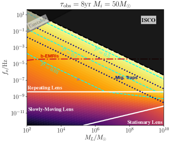
Figure 5: The same as Figure 1, except we draw characteristic locations of the outer-binary orbit in the migration trap (dark-blue dashed lines) and binary-EMRI (red dot-dashed line) scenarios discussed in the text.

IV.2.2 The AGN channel and migration traps

Within the AGN channel for merging BBHs (e.g., McKernan et al., 2018), gaseous torques can migrate BHs through an AGN disk. Within some models of AGN disks, peaks in the disk density profile can cause torques with opposite signs outward and inward of the density peak. This causes a radial migration trap that can bring two BHs to the location of the trap where they can merge, and even build up larger, second generation mergers (Bellovary et al., 2016; Secunda et al., 2018; Yang et al., 2019). Figure 5 replicates Figure 1 but includes the location of two possible migration traps from the literature, drawn as dark-blue dotted lines. These traps are located at $49$ and $662$ gravitational radii from the central SMBH (Sirko and Goodman, 2003). If the migration traps can hold the outer binary, and if gas forces do not merge the inner binary too quickly, then such migration trap binaries would have a high probability of exhibiting repeating-GW-lens flares, as well as a strong Doppler boost signature. Hence, lensing could also be a powerful discriminator for migration traps, and the AGN channel in general.

IV.2.3 binary-EMRI capture

In the tidal capture scenario, a binary black hole in the vicinity of a SMBH passes close to the tidal break-up radius of the binary on an eccentric orbit. Orbital energy is taken from the outer binary and traded to the inner binary, causing the inner binary to become eccentric. The outer binary circularizes to the original outer-pericenter distance of tens of SMBH gravitational radii, while the inner binary circularizes more slowly and can be emitting GWs in the LISA band. (Chen and Han, 2018; Chen et al., 2019). Depending on the detectable lifetime of the inner binary in the LISA band, such tidal captures would have a high probability of being lensed because of the tight orbit of the inner BBH around the SMBH. In Figure 5 we plot this b-EMRI capture radius (red dot-dashed line) for our fiducial $50{M_{\odot}}$ BBH with equal mass components.

We note that in both the b-EMRI and migration trap channels, the outer binary can be compact enough for detection of GWs by LISA or a future Deci-hertz GW detector. Lensing and the Doppler boost of GWs could be used to link the inner and outer binary GW signals to each other. We leave further exploration of this fascinating prospect to future work.

V Discussion

While the current predictions for the number of LISA stellar-mass BBHs detectable with pre-warning ability for the ground-based detectors number only in the few to tens, the BBH inspirals that can be uncovered in LISA at lower SNR from known LIGO mergers could number in the hundreds (Sesana, 2016; Kremer et al., 2019; Gerosa et al., 2019). Hence, the best case $\mathcal{O}(1\%)$ lensing predictions of the previous section are promising. The detection of a repeating-lens event would confirm that some BBHs merge in the environments of nuclear star clusters, close to the central SMBH. Depending on the occurrence rate, lensing detection would constrain the fraction of BBH mergers taking place in nuclear star cluster, $\xi$. Coupled with measurements of binary parameters such as eccentricity, lensing detections could also constrain the processes within a nuclear star cluster that lead to merger. That is, each of the specific merger scenarios discussed in §IV suggest different outer-binary orbital distributions as well as expected inner-and outer-binary eccentricities.

For example, single-single capture, binary-tidal capture, and the Kozai-Lidov mechanism can generate highly eccentric BBH inspirals in nuclear star clusters (O’Leary et al., 2009; Chen and Han, 2018; Nishizawa et al., 2017; Randall and Xianyu, 2018; Fragione et al., 2019). However, so can resonant three-body processes in the BH cores of globular clusters (e.g. Samsing, 2018; Rodriguez et al., 2018; D’Orazio and Samsing, 2018; Samsing and D’Orazio, 2018). Hence, it could be difficult to use binary parameter statistics alone to disentangle these different formation scenarios. However, a lensing detection would allow measurement of the central SMBH mass (e.g. Takahashi and Nakamura, 2003) and imply that the merger is occurring next to a SMBH in the nuclear cluster at the center of a galaxy, rather than in a globular cluster. From Doppler and lensing information we will also know the size (up to the redshift) and shape of the outer orbit, allowing to vet the efficiency of secular effects on the BBH inspiral, or compare to predictions from gas migration and binary tidal capture.

Even for the non-detection of lensing events, $\mathcal{O}(100)$ LISA detections of unlensed BBHs would begin to constrain the fraction of BBH mergers occurring in nuclear star clusters, and the distribution of mergers in such clusters.

As this work aims simply to point out the novelty and non-negligible occurrence of repeating-lens events, we have not computed differential SNRs for GW signals with and without lensing, and we have not computed the accuracy of parameter recovery from lensed waveforms. These of course, will depend on the SNR of the event, and so recovery of the lensing signature will depend on the redshift of the source. However, Ref. Wong et al. (2019) show that for triple systems similar to the example repeating-lens system displayed in Figure 2, and generally those with year outer-orbital timescales, have a detectable Doppler-boost signature (for non-face-on outer-orbital orientations) for which the orbital period can be recovered at $1\%$ precision (for an $\text{SNR}=10$ detection). With a detection of the Doppler boost and such a precise determination of the outer-orbital period, the time of a putative flare can be specified for recovery from the LISA data stream. Furthermore, a $\sim 1.5$ increase in amplitude over the course of hours to days, for an already detected BBH inspiral, is very likely discernible as it would be equivalent to a $\sim 30\%$ change in the inferred chirp mass for an unlensed waveform, whereas the chirp mass relative error determination is projected to be of order one part in a million (Sesana, 2016). Analysis of detection and parameter recovery for repeating-lens events should be carried out in future work.

For simplicity, we have considered only circular orbits for both binaries. However, both inner- and outer-binary orbits could be eccentric. Here we briefly discuss how eccentricity could affect our results. For an eccentric binary, the decay time will be shorter for the same outer-orbital period, meaning that the green line in Figure 1 will be moved downwards and the lensing probabilities presented in Figure 4 will saturate at longer observational timescales. Typically, for average outer binary eccentricities of $e\lesssim 0.5$, the decrease in orbital decay time is less then a factor of three and our results are not changed significantly. Eccentricity of the outer binary will also affect the shape of the lensing flares plus Doppler signature in a predictable way that is presented for EM lensing in Hu et al. (2019).

Eccentricity of the inner binary will also cause the inner binary to merge more quickly. As discussed in §IV.2.1, highly eccentric BBHs formed through GW capture could merge more quickly than an outer-orbital time, greatly reducing the lensing probability. These mergers will likely have an eccentricity signature in the LIGO 3rd generation or DECIGO bands (O’Leary et al., 2009; Samsing et al., 2019); evidence of high eccentricity, in conjunction with non-detection of lensing events, could corroborate such a scenario.

Eccentric inner binaries will also emit GWs at multiple higher harmonics of the binary orbital frequency. Hence, the same binary will be lensed differently for different harmonics because the value of $\chi$ in the lensing magnification (Eq. 7) is different for each harmonic. For high-SNR lensing events where multiple harmonics can be detected, propagation of GWs in the wave and geometrical optics limit could be observed simultaneously. We note, however, that the spread of GW power into higher harmonics could result in lower SNRs for highly eccentric systems.

Finally, eccentricity of either binary will act to destabilize the triple, resulting in the gray forbidden region in Figures 1 and 5 moving downwards. However, as stability only affects very compact outer orbits, the shorter decay times of eccentric binaries will likely affect our results before stability becomes an issue.

Further study of the effects of eccentricity and the eccentricity inducing Kozai-Lidov mechanism on our results is warranted in a future study. It may be especially important to include higher order relativistic effects (e.g. Liu et al., 2019) in the regimes important for repeated lensing.

Figure 4 also shows the expected lensing rate for more massive BBH mergers, up to $M_{i}=1000{M_{\odot}}$. While lensing of these more massive mergers is less probable, it may be that many more can be detected by LISA. LISA is the most sensitive to such $10^{3}-10^{4}{M_{\odot}}$ mergers and could detect them out to redshifts of $z\sim 10^{2}$ (Jani et al., 2019). If intermediate mass BH (IMBH) mergers occur close to SMBHs in hierarchical triples, e.g. through IMBH delivery via devoured globular clusters (Ebisuzaki et al., 2001; Fragione et al., 2018), or through BH build-up in migration traps (Bellovary et al., 2016), then lensing would be a common feature in the IMBH mergers detected in the LISA band.

At the opposite end of the mass spectrum, binary neutron star, or binary white dwarf mergers could be detected by LISA within the galaxy (Kremer et al., 2018). Hence, if such mergers occur in nearby globular clusters harboring a putative IMBH, or the galactic center, they could also be lensed.

While we have stressed the utility of lensing events to elucidate astrophysical channels for BBH formation and evolution, we note also that observing repeating lensing of GWs emitted from a BBH as it evolves in orbital frequency and possibly eccentricity could allow novel tests of GW propagation.

For example, the lens magnification was derived under the assumption that the GWs propagate following a linear wave equation in the weak field. If this is violated by, e.g. MONDIAN theories of gravity that predict non-linear propagation, then the magnification predicted here could also be altered (see e.g. Chesler and Loeb, 2017; Nishizawa, 2018). Such changes to the lensing waveforms can be worked out within a chosen modified theory. Additionally, the oscillation of the lensed amplitude of GWs seen in both types of lensing events in Figure 2 is set by the GW time delay. If GWs do not travel at the speed of light, or interact with themselves or the background spacetime non-linearly, one might expect this delay time to be altered, and so directly observable from a GW lensing event.

Such tests may be especially interesting when lensing can be observed in both the wave and geometrical optics regimes for the same GW source. Comparison of the two regimes can occur at different times over the evolution of the BBH in frequency, or in a simultaneous manner for eccentric binaries emitting GWs at multiple harmonics.

We have not treated changes in the polarization tensor of the GW due to lensing. These changes come in at the order of the lensing potential experienced by the propagating GWs, which is assumed to be much smaller than unity in the derivation of the lensing magnification (Takahashi and Nakamura, 2003). In situations where the source of GWs is within tens of gravitational radii from the SMBH however, polarization effects could enter at the few to ten percent level and could offer another probe of the central SMBH spacetime.

Finally, we note that electromagnetic lensing could occur if the BBH emits light, as might occur in the AGN channel. In that case, it is usually assumed that the AGN outshines the accretion powered luminosity generated by the inner BBH. However, if the lensing+Doppler period is already known, then a targeted search for that AGN periodicity in the localized error box could help to identify the weak periodicity and hence the host AGN. This would work similarly to a lock-in amplifier where the signal dithering is generated by the outer-binary orbit. The fractional amplitude of modulation that could be recovered would be proportional to the precision at which the outer-binary period can be determined from the GW lensing plus Doppler signature. This would also allow a direct comparison of the lensing of light and GWs as a test of the equivalence principle (Haiman, 2017) and also isolate the electromagnetic emission coming from accretion onto the BBH as opposed to accretion onto the SMBH.

VI Conclusions

We have shown that inspiraling BBHs that emit GWs in the LISA band and orbit a tertiary SMBH in a hierarchical triple with of order one year outer orbital periods, have up to a percent probability of being repeatedly strongly lensed by the SMBH. This lensing probability is only large when GWs from the inspiraling BBH can be observed for the orbital period of the BBH around the SMBH or longer and when the decay time of the BBH into the SMBH is of order a Hubble time or longer. The balance of the two sets the required $\mathcal{O}(\text{yr})$ orbital timescales. These short outer-orbital timescales can be populated for steep distributions of BBHs around the central SMBH ($dN/da_{0}\propto a^{-1}_{o}$ or steeper) that have been shown to occur for single-single GW capture scenarios or via migration traps in AGN disks, or through binary tidal capture by the central SMBH. LISA has the best chance of discovering such a repeating-lens event, because it will be able to detect inspiraling BBHs for the final years of their lives and because it could detect up to hundreds of such events (Sesana, 2016; Kremer et al., 2018; Gerosa et al., 2019, though fewer at high SNR).

The characteristic signature of these lensing events is magnification by a factor of $\sim 1.1\times$ to $2\times$ (cf. Eq. 7) of the GW amplitude for a duration of $\sim 0.01$ of the period of the BBH in its orbit around the SMBH (hours to days). The event will repeat once every outer-binary orbital period and be accompanied by detectable deviations in the GW phase due to the relativistic Doppler boost (e.g., Wong et al., 2019). A detection of this phenomenon will provide the mass of the central SMBH, helping to constrain BBH formation scenarios, specifically pointing to formation in nuclear star clusters. Detection of time and frequency variable lensing of GWs could also provide a new testing ground for theories of gravity. Non-detection will put upper limits on the fraction of BBHs formed in the vicinity of SMBHs and the astrophysical processes that form them.

Appendix A Effect of the Doppler Boost on the GW Amplitude

We sketch a derivation of the relativistic Doppler boost formula for GWs, ignoring at first any cosmological redshift. We consider a GW in the time domain with frequency $f$, amplitude $|h(t(f))|$ and phase $\phi(t(f))$ (for notational simplicity, we will write $|h(f)|$ hereafter). We do not consider the detection of different GW polarizations, although see Ref. Torres-Orjuela et al. (2018).

In the rest frame of the GW emitting source the GW frequency at any time is given by $f_{\text{em}}$. In the frame of an observer for which the source has a relative speed $\beta=v/c$ with a fraction $\beta_{||}$ along the line of sight, the observed GW frequency is $f_{\text{obs}}=Df_{\text{em}}$, where the Doppler factor $D$ is,

$$D \equiv\left[\gamma\left(1-\beta_{||}\right)\right]^{-1}$$ (17)

with $\gamma=\left(1-\beta^{2}\right)^{-1/2}$. Then the measured phase of the wave changes over time due to the Doppler boost. The phase accumulated over an observation time of length $\tau$ is

$$\phi(\tau)=\int^{t_{0}+\tau}_{t_{0}}{\pi Df_{\text{em}}dt}.$$ (18)

which has been considered in many other works (see Ref. Wong et al., 2019, and references therein)

We also consider the effect of the Doppler boost on the wave amplitude. Just as for electromagnetic waves, we use that the photon/graviton occupation number is Lorentz invariant,

$$\frac{I_{E}}{E^{3}}=\frac{I_{f}}{f^{3}}=\text{Invar.},$$ (19)

where $E$ is the energy of a photon or graviton, $f$ is the wave frequency and the first equality makes the assumption that the energy and frequency of a gravitational wave are related linearly (if they are not, the observed Doppler boost of GWs would recover this). $I_{f}$ is the specific intensity of the radiation.

For GWs, occupation number is still a Lorentz invariant and the transformation of the specific intensity still holds, but we are interested in the transformation of the wave amplitude $|h(f)|$. The specific intensity and $|h(f)|$ are related by

$$|h(f)|^{2}=\frac{\pi c^{3}}{4G}f^{-2}\frac{dE}{dAdt}=\frac{\pi c^{3}}{4Gf^{2}}\int{I_{f}\ d\Omega df},$$ (20)

and for gravitational waves we can write,

$$I_{f}\equiv\frac{dE_{n}}{dAdtd\Omega df}=\frac{1}{4\pi r^{2}(z)}\frac{dP}{d\Omega}\delta\left(f-nf_{K}\right)$$ (21)

where $dP/d\Omega$ is the angle dependent emitted power, $f_{K}$ is the Keplerian orbital frequency, and GWs are emitted with frequency at the $n^{\text{th}}$ harmonic of $f_{K}$. Using that $I_{f\text{obs}}=D^{3}I_{f,\text{em}}$, $d\Omega_{\text{obs}}=D^{-2}d\Omega_{\text{em}}$, $df_{\text{obs}}=Ddf_{\text{em}}$ and integrating we find,

$$|h(f_{\text{obs}})|^{2}_{n,\text{obs}} = |h(f_{\text{obs}}/D)|^{2}_{n,\text{em}}.$$ (22)

This may also be found by simply transforming the first quantity in Eq. (20), using that $dE_{\text{obs}}=DdE_{\text{em}}$, $dA_{\text{obs}}=dA_{\text{em}}$, and $dt_{\text{obs}}=D^{-1}dt_{\text{em}}$.

Dropping the $n$ subscript, the characteristic strain, $h^{2}_{c}(f)=|h(f)|^{2}f^{2}/\dot{f}$, transforms the same as $|h(f)|$ because $\dot{f}_{\text{obs}}=D^{2}\dot{f}_{\text{em}}$, that is, the number of cycles per frequency bin is invariant. The Fourier transform of the strain amplitude is given by $|\tilde{h}(f_{\text{obs}})|^{2}_{\text{obs}}=D^{-2}|\tilde{h}(f_{\text{obs}}/D)|^{2}_{\text{em}}$, where the extra factor of $D^{-2}$ from Eq. (22) simply accounts for the extra factor of $\dot{f}$ in $|\tilde{h}(f)|^{2}$.

Hence, the transformation of the strain amplitude does not explicitly contain the Doppler factor, but the amplitude is altered by its dependence on the frequency. This frequency dependence arises for the same reason that the electromagnetic Doppler formula is written with a $D^{3-\alpha}$ dependence for a specific intensity that goes as $f^{-\alpha}$, and for the same reason that the redshifted GW amplitude depends on the luminosity distance and not the co-moving distance.

We can then write the strain amplitude for the inner-binary in terms of observed quantities as,

$$|h_{i}|\propto D\frac{\mathcal{M}^{5/3}_{i}f^{2/3}_{i}}{d(z)}g(I_{i}),$$ (23)

where $g(I_{i})$ is the inclination dependence of the inner binary and $d(z)$ is the luminosity distance to the source. This follows from the relations

$$f=\frac{D}{1+z}f_{\text{em}},\quad\dot{f}=\left(\frac{D}{1+z}\right)^{2}\dot{f}_{\text{em}},$$

$$\mathcal{M}\propto\dot{f}^{3/5}f^{-11/5}.$$ (24)

References

- The LIGO Scientific Collaboration et al. (2018) The LIGO Scientific Collaboration, the Virgo Collaboration, B. P. Abbott, R. Abbott, T. D. Abbott, S. Abraham, F. Acernese, K. Ackley, C. Adams, and R. X. Adhikari, arXiv e-prints arXiv:1811.12907 (2018), eprint 1811.12907.
- The LIGO Scientific Collaboration and the Virgo Collaboration (2018) The LIGO Scientific Collaboration and the Virgo Collaboration, arXiv e-prints arXiv:1811.12940 (2018), eprint 1811.12940.
- Yunes et al. (2011) N. Yunes, B. Kocsis, A. Loeb, and Z. Haiman, Phys. Rev. Lett. 107, 171103 (2011), eprint 1103.4609.
- Kocsis et al. (2011) B. Kocsis, N. Yunes, and A. Loeb, PRD 84, 024032 (2011), eprint 1104.2322.
- Fedrow et al. (2017) J. M. Fedrow, C. D. Ott, U. Sperhake, J. Blackman, R. Haas, C. Reisswig, and A. De Felice, Phys. Rev. Lett. 119, 171103 (2017), eprint 1704.07383.
- D’Orazio and Loeb (2018) D. J. D’Orazio and A. Loeb, PRD 97, 083008 (2018), eprint 1706.04211.
- Derdzinski et al. (2019) A. M. Derdzinski, D. D’Orazio, P. Duffell, Z. Haiman, and A. MacFadyen, MNRAS 486, 2754 (2019), eprint 1810.03623.
- LIGO Scientific Collaboration and the Virgo Collaboration (2018) LIGO Scientific Collaboration and the Virgo Collaboration, Phys. Rev. Lett. 121, 161101 (2018), eprint 1805.11581.
- Meiron et al. (2017) Y. Meiron, B. Kocsis, and A. Loeb, ApJ 834, 200 (2017), eprint 1604.02148.
- Kocsis et al. (2006) B. Kocsis, Z. Frei, Z. Haiman, and K. Menou, ApJ 637, 27 (2006), eprint astro-ph/0505394.
- Bonvin et al. (2017) C. Bonvin, C. Caprini, R. Sturani, and N. Tamanini, PRD 95, 044029 (2017), eprint 1609.08093.
- Chen et al. (2019) X. Chen, S. Li, and Z. Cao, MNRAS 485, L141 (2019), eprint 1703.10543.
- Inayoshi et al. (2017) K. Inayoshi, N. Tamanini, C. Caprini, and Z. Haiman, PRD 96, 063014 (2017), eprint 1702.06529.
- Robson et al. (2018) T. Robson, N. J. Cornish, N. Tamanini, and S. Toonen, PRD 98, 064012 (2018), eprint 1806.00500.
- Wong et al. (2019) K. W. K. Wong, V. Baibhav, and E. Berti, MNRAS 488, 5665 (2019), eprint 1902.01402.
- Randall and Xianyu (2019) L. Randall and Z.-Z. Xianyu, ApJ 878, 75 (2019), eprint 1805.05335.
- Takahashi and Nakamura (2003) R. Takahashi and T. Nakamura, ApJ 595, 1039 (2003), eprint astro-ph/0305055.
- Ruffa (1999) A. A. Ruffa, ApJL 517, L31 (1999).
- Christian et al. (2018) P. Christian, S. Vitale, and A. Loeb, PRD 98, 103022 (2018), eprint 1802.02586.
- Kocsis (2013) B. Kocsis, ApJ 763, 122 (2013), eprint 1211.6427.
- Antonini and Perets (2012) F. Antonini and H. B. Perets, ApJ 757, 27 (2012), eprint 1203.2938.
- Chen and Han (2018) X. Chen and W.-B. Han, Condensed Matter Physics 1, 53 (2018), eprint 1801.05780.
- Fernández and Kobayashi (2018) J. J. Fernández and S. Kobayashi, arXiv e-prints (2018), eprint 1805.09593.
- Bellovary et al. (2016) J. M. Bellovary, M.-M. Mac Low, B. McKernan, and K. E. S. Ford, ApJL 819, L17 (2016), eprint 1511.00005.
- Stone et al. (2017) N. C. Stone, B. D. Metzger, and Z. Haiman, MNRAS 464, 946 (2017), eprint 1602.04226.
- Bartos et al. (2017) I. Bartos, B. Kocsis, Z. Haiman, and S. Márka, ApJ 835, 165 (2017), eprint 1602.03831.
- McKernan et al. (2018) B. McKernan, K. E. S. Ford, J. Bellovary, N. W. C. Leigh, Z. Haiman, B. Kocsis, W. Lyra, M. M. Mac Low, B. Metzger, M. O’Dowd, et al., ApJ 866, 66 (2018), eprint 1702.07818.
- Amaro-Seoane and et al. (2017) P. Amaro-Seoane and et al., ArXiv e-prints (2017), eprint 1702.00786.
- Chesler and Loeb (2017) P. M. Chesler and A. Loeb, Phys. Rev. Lett. 119, 031102 (2017), eprint 1704.05116.
- Mardling and Aarseth (2001) R. A. Mardling and S. J. Aarseth, MNRAS 321, 398 (2001).
- Schneider et al. (1992) P. Schneider, J. Ehlers, and E. E. Falco, Gravitational Lenses (1992).
- D’Orazio and Di Stefano (2018) D. J. D’Orazio and R. Di Stefano, MNRAS 474, 2975 (2018), eprint 1707.02335.
- D’Orazio and Di Stefano (2019) D. J. D’Orazio and R. Di Stefano, arXiv e-prints arXiv:1906.11149 (2019), eprint 1906.11149.
- Sesana (2016) A. Sesana, Phys. Rev. Lett. 116, 231102 (2016), eprint 1602.06951.
- Robson et al. (2019) T. Robson, N. J. Cornish, and C. Liu, Classical and Quantum Gravity 36, 105011 (2019), eprint 1803.01944.
- http://www.et gw.eu/ (2018) T. E. T. P. http://www.et gw.eu/ (2018).
- Sesana et al. (2005) A. Sesana, F. Haardt, P. Madau, and M. Volonteri, ApJ 623, 23 (2005), eprint astro-ph/0409255.
- D’Orazio and Samsing (2018) D. J. D’Orazio and J. Samsing, MNRAS 481, 4775 (2018), eprint 1805.06194.
- Bahcall and Wolf (1976) J. N. Bahcall and R. A. Wolf, ApJ 209, 214 (1976).
- Bahcall and Wolf (1977) J. N. Bahcall and R. A. Wolf, ApJ 216, 883 (1977).
- O’Leary et al. (2009) R. M. O’Leary, B. Kocsis, and A. Loeb, MNRAS 395, 2127 (2009), eprint 0807.2638.
- Shankar et al. (2004) F. Shankar, P. Salucci, G. L. Granato, G. De Zotti, and L. Danese, MNRAS 354, 1020 (2004), eprint astro-ph/0405585.
- Samsing et al. (2019) J. Samsing, D. J. D’Orazio, K. Kremer, C. L. Rodriguez, and A. Askar, arXiv e-prints arXiv:1907.11231 (2019), eprint 1907.11231.
- Chen and Amaro-Seoane (2017) X. Chen and P. Amaro-Seoane, ApJL 842, L2 (2017), eprint 1702.08479.
- Secunda et al. (2018) A. Secunda, J. Bellovary, M.-M. Mac Low, K. E. S. Ford, B. McKernan, N. Leigh, and W. Lyra, arXiv e-prints (2018), eprint 1807.02859.
- Yang et al. (2019) Y. Yang, I. Bartos, V. Gayathri, S. Ford, Z. Haiman, S. Klimenko, B. Kocsis, S. Márka, Z. Márka, B. McKernan, et al., arXiv e-prints arXiv:1906.09281 (2019), eprint 1906.09281.
- Sirko and Goodman (2003) E. Sirko and J. Goodman, MNRAS 341, 501 (2003), eprint astro-ph/0209469.
- Tang et al. (2017) Y. Tang, A. MacFadyen, and Z. Haiman, MNRAS 469, 4258 (2017), eprint 1703.03913.
- Muñoz et al. (2019) D. J. Muñoz, R. Miranda, and D. Lai, ApJ 871, 84 (2019), eprint 1810.04676.
- Duffell et al. (2019) P. C. Duffell, D. D’Orazio, A. Derdzinski, Z. Haiman, A. MacFadyen, A. L. Rosen, and J. Zrake, arXiv e-prints arXiv:1911.05506 (2019), eprint 1911.05506.
- Kremer et al. (2019) K. Kremer, C. L. Rodriguez, P. Amaro-Seoane, K. Breivik, S. Chatterjee, M. L. Katz, S. L. Larson, F. A. Rasio, J. Samsing, C. S. Ye, et al., PRD 99, 063003 (2019), eprint 1811.11812.
- Gerosa et al. (2019) D. Gerosa, S. Ma, K. W. K. Wong, E. Berti, R. O’Shaughnessy, Y. Chen, and K. Belczynski, PRD 99, 103004 (2019), eprint 1902.00021.
- Nishizawa et al. (2017) A. Nishizawa, A. Sesana, E. Berti, and A. Klein, MNRAS 465, 4375 (2017), eprint 1606.09295.
- Randall and Xianyu (2018) L. Randall and Z.-Z. Xianyu, ApJ 853, 93 (2018), eprint 1708.08569.
- Fragione et al. (2019) G. Fragione, E. Grishin, N. W. C. Leigh, H. B. Perets, and R. Perna, MNRAS 488, 47 (2019), eprint 1811.10627.
- Samsing (2018) J. Samsing, PRD 97, 103014 (2018), eprint 1711.07452.
- Rodriguez et al. (2018) C. L. Rodriguez, P. Amaro-Seoane, S. Chatterjee, K. Kremer, F. A. Rasio, J. Samsing, C. S. Ye, and M. Zevin, PRD 98, 123005 (2018), eprint 1811.04926.
- Samsing and D’Orazio (2018) J. Samsing and D. J. D’Orazio, MNRAS 481, 5445 (2018), eprint 1804.06519.
- Hu et al. (2019) B. X. Hu, D. J. D’Orazio, Z. Haiman, K. L. Smith, B. Snios, M. Charisi, and R. Di Stefano, arXiv e-prints arXiv:1910.05348 (2019), eprint 1910.05348.
- Liu et al. (2019) B. Liu, D. Lai, and Y.-H. Wang, ApJL 883, L7 (2019), eprint 1906.07726.
- Jani et al. (2019) K. Jani, D. Shoemaker, and C. Cutler, arXiv e-prints arXiv:1908.04985 (2019), eprint 1908.04985.
- Ebisuzaki et al. (2001) T. Ebisuzaki, J. Makino, T. G. Tsuru, Y. Funato, S. Portegies Zwart, P. Hut, S. McMillan, S. Matsushita, H. Matsumoto, and R. Kawabe, ApJL 562, L19 (2001), eprint astro-ph/0106252.
- Fragione et al. (2018) G. Fragione, I. Ginsburg, and B. Kocsis, ApJ 856, 92 (2018), eprint 1711.00483.
- Kremer et al. (2018) K. Kremer, S. Chatterjee, K. Breivik, C. L. Rodriguez, S. L. Larson, and F. A. Rasio, Phys. Rev. Lett. 120, 191103 (2018), eprint 1802.05661.
- Nishizawa (2018) A. Nishizawa, PRD 97, 104037 (2018), eprint 1710.04825.
- Haiman (2017) Z. Haiman, PRD 96, 023004 (2017), eprint 1705.06765.
- Torres-Orjuela et al. (2018) A. Torres-Orjuela, X. Chen, Z. Cao, P. Amaro-Seoane, and P. Peng, arXiv e-prints (2018), eprint 1806.09857.