The Possible Astrometric Signature of a Planetary-mass Companion to the Nearby Young Star TW Piscis Austrini (Fomalhaut B): Constraints from Astrometry, Radial Velocities, and Direct Imaging

Abstract

We present constraints on the presence of substellar companions to the nearby ($d\sim 7.6$ pc), young ($440\pm 40$ Myr) K4Ve star TW Piscis Austrini, the wide ($\sim$0.3 pc) companion to the A4V star Fomalhaut. We combined absolute astrometry from Hipparcos and Gaia with literature radial velocity measurements and dedicated high-contrast imaging observations obtained with Keck/NIRC2 to achieve sensitivity to brown dwarf and planetary-mass companions ($\gtrsim 2$ M_Jup) over many decades of orbital period ($\lesssim 10^{3}$ yr). The significant astrometric acceleration measured between the Hipparcos and Gaia catalogues, reported previously in the literature, cannot be explained by the orbital motion of TW PsA around the barycenter of the Fomalhaut triple system. Instead, we find that it is consistent with the reflex motion induced by an orbiting substellar companion. The combination of astrometry, radial velocities, and a deep $L^{\prime}$ imaging dataset leads to a constraint on the companion mass of $1.2_{-0.6}^{+0.7}$ M_Jup. However, the period of the companion is poorly constrained, with a highly multi-modal period posterior distribution due to aliasing with the 24.25 year baseline between Hipparcos and Gaia. If confirmed through continued astrometric or spectroscopic monitoring, or via direct detection, the companion to TW PsA would represent a choice target for detailed atmospheric characterization with high-contrast instruments on the upcoming James Webb Space Telescope and Wide Field Infrared Survey Telescope.

1 Introduction

The field of astrometric detection of exoplanets will soon be transformed with the discovery of thousands of planetary-mass companions via the astrometric reflex motion induced on their host star measured by Gaia (Perryman et al., 2014). While these discoveries will span a wide range of orbital periods, a small subset of them will be at separations wide enough, and around stars young enough, that they will be amenable to direct detection and characterization with ground- and space-based instrumentation. Previous ground-based surveys searching for the astrometric signal induced by an orbiting planet have typically targeted fainter stars due to the requirement to have similar-magnitude reference stars (e.g., Sahlmann et al., 2014), whilst space-based observations have focused on characterizing known systems (e.g., Benedict et al., 2017). These observations are typically expensive, and dedicated astrometric missions such as Gaia are required to have sufficient sensitivity around a large enough number of stars for a blind search to be worthwhile. While we await the release of the final Gaia astrometric catalog, the intermediate data releases (e.g. Gaia Collaboration et al., 2018) can be combined with previous measurements from Hipparcos to search for planetary-mass companions to nearby stars (e.g. Brandt, 2018; Kervella et al., 2019).

TW Piscis Austrini (catalog ) (TW PsA) is a K4Ve star (Keenan & McNeil, 1989) at a distance of 7.6 pc (Gaia Collaboration et al., 2018). It shares a similar three-dimensional velocity to the naked-eye star Fomalhaut (catalog ) (Luyten, 1938) and the faint M-dwarf LP 876-10 (catalog ) (Mamajek et al., 2013), forming a wide triple system that extends several degrees across the sky. The Fomalhaut system is young, with an estimated age of $440\pm 40$ Myr (Mamajek, 2012). This system has been well-studied given its proximity. The primary hosts an extended debris disk (Holland et al., 1998), within which a candidate exoplanet with a circumplanetary dust ring has been detected via direct imaging at optical wavelengths (Kalas et al., 2008). LP 876-10 also hosts a debris disk (Kennedy et al., 2014), unusual given the apparent rarity of debris disks around M-dwarfs. Thermal-infrared measurements of TW PsA between 24 and 100 $\mu$m do not any show evidence of emission in excess of the predicted photospheric flux (Carpenter et al., 2008; Kennedy et al., 2014). Shannon et al. (2014) propose that all three stars originate from the same birth cluster, with Fomalhaut and LP 876-10 forming as a binary and TW PsA captured from the cluster into a weakly bound orbit. While Fomalhaut shows evidence of a planetary system (Kalas et al., 2008), searches for giant planets around TW PsA via direct imaging (Heinze et al., 2010; Durkan et al., 2016; Nielsen et al., 2019) and radial velocity (Butler et al., 2017) have thus far yielded nothing.

In this paper we present constraints on the presence of wide-orbit giant planets around TW PsA with a joint analysis of absolute astrometry from Hipparcos and Gaia, a deep high-contrast imaging dataset, and a long-term radial velocity record. We discuss the measured astrometric acceleration, previously noted by (Kervella et al., 2019), in Section 2, where we demonstrate it cannot be explained by the orbit of TW PsA around Fomalhaut, and present limits on the period and mass of an orbiting companion consistent with the measured acceleration. The long-term radial velocity record is presented in Section 3, and the deep coronagraphic imaging dataset in Section 4. Finally, we present joint constraints on the properties of a companion consistent with the astrometric signal in Section 5.

2 Astrometry

Absolute astrometry for TW PsA was included in both the Hipparcos (HIP 113283; ESA, 1997; van Leeuwen, 2007a) and the recent Gaia (Gaia DR2 6604147121141267712; Gaia Collaboration et al., 2018) catalogues. In the Hipparcos catalogue, the star appears typical compared to other stars within a factor of two in $H_{\rm p}$-band flux. The catalogue goodness of fit metric is $1.33$ compared to $1.30_{-1.39}^{+2.19}$ for the similar brightness stars. This metric is equivalent to $\chi^{2}=99.5$ for TW PsA, ($\chi^{2}=131_{-47}^{+71}$ for the comparison sample), corresponding to a $\chi^{2}_{\nu}=1.2$ given the 87 one-dimensional astrometric measurements of the star and the five model parameters. The quality of fit was good enough that no attempt was made to fit either additional acceleration terms or a stochastic solution (van Leeuwen, 2007b).

We performed a similar check of the quality of the astrometry in the Gaia Data Release 2 catalogue. We selected stars within a factor of two in $G$-band flux, that had good quality parallax and photometric measurements as in Lindegren et al. (2018). The goodness of fit metric for TW PsA was unusually low at 4.7 compared with $19.1_{-9.7}^{+35.1}$ for stars in the comparison sample, indicating a relatively good quality of fit of the five parameter model to the astrometric measurements ($\chi^{2}=136$ for TW PsA and $\chi^{2}=960_{-530}^{+3560}$ for the comparison sample). The reduced $\chi^{2}$ is somewhat high, $\chi^{2}_{\nu}=2.0$ ($\chi^{2}_{\nu}=4.3_{-1.9}^{+15.7}$ for the comparison sample), suggesting that the uncertainties on the individual astrometric measurements are slightly underestimated. No significant astrometric excess noise was reported in the catalogue.

2.1 Astrometric acceleration

The acceleration of TW PsA between the Hipparcos and Gaia missions was estimated by computing three proper motion differentials; (1) $\mu_{\rm G}-\mu_{\rm H}$ the difference between the two catalogue proper motions, (2) $\mu_{\rm H}-\mu_{\rm HG}$ the difference between the proper motion computed from the absolute position of the star in the two catalogues and the Hipparcos proper motion, and (3) $\mu_{\rm G}-\mu_{\rm HG}$ the same but with respect to the Gaia proper motion. The proximity of TW PsA (7.6 pc) causes a non-negligible change in its apparent proper motion across the sky simply due to perspective effects. Without correcting for these, the estimated position of the star at the Gaia epoch using Hipparcos astrometry will be systematically offset by 0.2 mas, biasing the derived $\mu_{\rm HG}$ proper motion by $\sim$10 $\mu$as yr^-1. The magnitude of this effect is comparable to the size of the uncertainty on $\mu_{\rm HG}$ given the precision of the absolute astrometric measurement of the star within both catalogues.

We account for this effect using the prescription laid out in Butkevich & Lindegren (2014), propagating the Hipparcos astrometry from the Hipparcos to the Gaia epoch (and vice versa) before computing the difference. Rather than simply dividing the offset between the Hipparcos and Gaia coordinates by the 24.25 yr baseline, $\mu_{\rm HG}$ was instead calculated numerically using a Monte Carlo algorithm given the measurement and uncertainty on the absolute positions of the star at the two epochs and the propagation formalism described in Butkevich & Lindegren (2014). We assumed that the parallax and radial velocity of the star did not change significantly over the 24.25-year baseline.

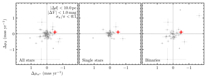
Figure 1: The acceleration measured using the Gaia proper motion $\mu_{\rm G}$ and that derived from the absolute position in the Hipparcos and Gaia catalogues $\mu_{\rm HG}$ for a sample of stars sharing similar properties to TW PsA (red symbol). The three panels show all stars (left), those that are thought to be single (middle), and those with evidence of binarity (right). The binary sample contains stars with proper motion differentials of up to 140 mas yr^-1 (17 of the sample are outside of the plotting window), whereas no star in the single sample has an amplitude greater than 1.1 mas yr^-1.

We performed a similar analysis on 106 nearby ($<17$ pc) stars that have good quality Hipparcos parallax measurements ($\sigma_{\pi}/\pi<0.1$) and that share a similar apparent magnitude to TW PsA ($|\Delta V|<1$ mag). We plot the $\mu_{\rm G}-\mu_{\rm HG}$ proper motion differential—the most precisely determined—for this sample in Figure 1. We created two sub-samples based on the binarity of each of the 106 stars; one consisting of the 53 stars that show some evidence of binarity in the literature (either from stellar, substellar, or degenerate companions), and another with those that to the best of our knowledge are single. TW PsA appears to be more discrepant with the majority of the stars in the single sub-sample that have accelerations clustered tightly around zero. The other outliers within the single star sample are likely host to massive companions that have yet to be discovered that are inducing an astrometric acceleration.

2.2 Orbital motion?

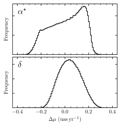
Figure 2: Change in the proper motion of TW PsA between the Hipparcos and Gaia epochs in the $\alpha^{\star}$ (top) and $\delta$ (bottom) directions induced by orbital motion around Fomalhaut, at a three-dimensional distance of $0.280_{-0.012}^{+0.019}$ pc. The gravitational influence of the distant companion LP 876-10 is assumed to be negligible.

TW PsA’s association with Fomalhaut was first suggested by Luyten (1938), and was later confirmed with Hipparcos astrometry by Shaya & Olling (2010); Mamajek (2012). The current projected separation of the two stars is almost two degrees on the sky, corresponding to a true separation of $0.280_{-0.012}^{+0.019}$ pc (Mamajek, 2012). The third component of this system is the M4 star LP 876-10, located at a projected separation of approximately six degrees (true separation of $0.77\pm 0.01$ pc) from Fomalhaut (Mamajek et al., 2013). Both of these stars lie within the tidal radius of Fomalhaut, and it is assumed that they form a gravitationally bound triple system. The barycenter of this system lies close to Fomalhaut A (1.92 M_⊙), given its mass relative to TW PsA (0.725 M_⊙; Demory et al., 2009) and LP 876-10 (0.18 M_⊙).

The orbital motion of TW PsA around Fomalhaut was noted by Kervella et al. (2019) as being a potential source of the astrometric acceleration measured between the Hipparcos and Gaia astrometry. The magnitude of the tangential velocity differential ($\Delta v_{\rm tan}=18.7\pm 6.4$ m s^-1, Kervella et al., 2019) seems inconsistent with the change in orbital velocity expected for an orbital period of close to 8 Myr (Mamajek, 2012). The escape velocity from Fomalhaut is estimated to be 210 m s^-1 (Mamajek, 2012), so it would be surprising for the velocity of TW PsA to change by close to 10% of the escape velocity in a negligible fraction of the orbital period.

We therefore investigated the plausible ranges of astrometric acceleration over the 24.25-year baseline between the Hipparcos and Gaia epochs induced by the orbital motion of TW PsA. For simplicity, we ignored the presence of the low-mass companion LP 876-10 and assumed that Fomalhaut and TW PsA formed a binary with no other massive companions in the system. While this assumption will lead to an imprecise determination of the acceleration induced by the orbit of TW PsA around the barycenter of the triple system, it will be sufficient for an order-of-magnitude estimate of the effect. Given the large angular separation between the two stars, we needed to determine their relative positions in a tangent plane within which the visual orbit could be fit. To achieve this we converted Hipparcos astrometry and literature radial velocities of the two stars into Cartesian coordinates in the ICRS frame. This coordinate system was then rotated so that the $yz$ plane was tangent to the celestial sphere at the mid-point between the two stars ($\alpha=22^{\rm h}57^{\rm m}1^{\rm s}.33$, $\delta=-30^{\circ}35^{\prime}36.63^{\prime\prime}$), with $+x$ pointing away from Earth.

We used rejection sampling (Blunt et al., 2017, 2019) to identify visual orbits consistent with the tangent plane separation ($\rho=54070\pm 160$ au) and position angle ($\theta=187.8805\pm 0.0002$ deg) of the pair. The tangent plane position and velocity of the companion from these accepted orbits were first rotated back into the standard ICRS frame and then converted into spherical coordinates to determine the relative parallax and proper motion for each accepted orbit. We then performed an additional rejection step to select only those orbits consistent with the relative parallax ($\Delta\pi=1.61\pm 0.78$ mas) and proper motion ($\Delta\mu_{\alpha^{\star}}=2.16\pm 0.82$ mas yr^-1, $\Delta\mu_{\delta}=5.69\pm 0.59$ mas yr^-1) of the two stars from the Hipparcos catalogue. Here we use the notation $\alpha^{\star}=\alpha\cos\delta$.

From these accepted orbits we calculated the expected change in the proper motion of TW PsA between the Hipparcos and Gaia epochs due to orbital motion alone. We find a $3\sigma$ upper limit for the amplitude of the acceleration due to orbital motion of 0.3 $\mu$as yr^-1 in both the $\alpha^{\star}$ and $\delta$ directions (Figure 2), corresponding to a tangential velocity change of $\Delta v_{\rm tan}<0.01$ m s^-1. While the visual orbit is still rather unconstrained due to the long orbital period ($5.8_{-2.2}^{+3.8}$ Myr, $4.5_{-1.2}^{+1.8}\times 10^{4}$ au), the inclination is marginally constrained $i=65_{-29}^{+30}$ deg, suggestive of a counter-clockwise orbit for TW PsA around Fomalhaut.

2.3 Inferred companion properties

The astrometry of TW PsA measured in the Hipparcos and Gaia epochs can be used to infer the range of periods and masses that are consistent with the measured astrometric acceleration. The framework is described in detail in De Rosa et al. 2019, submitted, but a brief summary will be given here. The astrometric model consists of eleven free parameters. Seven define the orbit of the companion that is perturbing the star; the total semi-major axis $a$, the inclination $i$, eccentricity $e$, argument of periastron $\omega$, longitude of the ascending node $\Omega$, epoch of periastron $\tau$ (in fractions of the orbital period), and the mass of the companion $M_{2}$. We assume a fixed mass for the primary of 0.725 M_⊙. The remaining parameters define the proper motion of the barycenter of the TW PsA system ($\mu_{\alpha^{\star}}$, $\mu_{\delta}$) and an offset for the photocenter position at the Hipparcos epoch to account for the catalogue uncertainties.

The location and instantaneous proper motion of the photocenter was calculated at both the Hipparcos and Gaia epochs by combining the constant motion of the barycenter with the photocenter orbit computed from the orbital elements. The displacement between the barycenter and photocenter was calculated using the mass ratio and flux ratio of the two stars. We used an empirical mass-magnitude relation (Pecaut & Mamajek, 2013) to estimate the absolute magnitude of TW PsA and the companion, if $M_{2}$ was above the stellar-substellar limit. The flux of companions with $M_{2}<0.077$ $M_{\odot}$ was assumed to be negligible. We corrected for perspective effects using the formalism outlined in Butkevich & Lindegren (2014), assuming a parallax of 131.438 mas and a radial velocity of 7.217 km s^-1 (Soubiran et al., 2013). We assume that the parallax and radial velocity are precisely determined to minimize the number of free parameters within the fit.

Table 1: Measurements and derived quantities in the astrometric model

Symbol	Unit	Description
$\Delta\alpha_{0}^{\star}$, $\Delta\delta_{0}$	mas	Offset between barycenter and Hipparcos catalogue position (1991.25)
$\alpha_{1}^{\star}$, $\delta_{1}$	mas	Predicted position of $G$-band photocenter (2015.5)
$\alpha_{\rm G}^{\star}$, $\delta_{\rm G}$	mas	Position of $G$-band photocenter measured by Gaia (2015.5)
$\mu_{\alpha^{\star}}$, $\mu_{\alpha^{\star}}$	mas yr-1	Proper motion of system barycenter (1991.25)
$\mu_{\alpha^{\star},0}$, $\mu_{\delta,0}$	mas yr-1	Orbital motion of photocenter around barycenter (1991.25)
$\mu_{\alpha^{\star},1}$, $\mu_{\delta,1}$	mas yr-1	Orbital motion of photocenter around barycenter (2015.5)
$\mu_{\alpha^{\star},{\rm H}}$, $\mu_{\delta,{\rm H}}$	mas yr-1	Proper motion measured by Hipparcos (1991.25)
$\mu_{\alpha^{\star},{\rm G}}$, $\mu_{\delta,{\rm G}}$	mas yr-1	Proper motion measured by Gaia (2015.5)

As in De Rosa et al. 2019, submitted, we used the parallel-tempered affine-invariant Markov chain Monte Carlo ensemble sampler emcee (Foreman-Mackey et al., 2013) to sample the posterior distributions of the eleven model parameters. We computed the likelihood $\ln{\mathcal{L}}=-\chi^{2}/2$ at each step in the chain by comparing the predicted position and proper motion of the photocenter at both the Hipparcos and Gaia epochs with the measurements from both catalogues as

$$\chi^{2}=R_{\rm H}^{\top}{\mathbf{C}}_{\rm H}^{-1}R_{\rm H}+R_{\rm G}^{\top}{\mathbf{C}}_{\rm G}^{-1}R_{\rm G}$$ (1)

with H and G subscripts denoting measurements of TW PsA from the Hipparcos and Gaia catalogues, respectively. The residual vectors $R$ were calculated as

$$\begin{split}R_{\rm H}=&[\Delta\alpha^{\star}_{0},\Delta\delta_{0},\\ &\mu_{\alpha}^{\star}+\mu_{\alpha^{\star},0}-\mu_{\alpha^{\star},{\rm H}},\mu_{\delta}+\mu_{\delta,0}-\mu_{\delta,{\rm H}}]\\ R_{\rm G}=&[(\alpha_{1}-\alpha_{\rm G})\cos\delta_{1},\delta_{1}-\delta_{\rm G},\\ &\mu_{\alpha}^{\star}+\mu_{\alpha^{\star},1}-\mu_{\alpha^{\star},{\rm G}},\mu_{\delta}+\mu_{\delta,1}-\mu_{\delta,{\rm G}}].\end{split}$$ (2)

The variables are described in Table 1. The covariance matrices ${\mathbf{C}}_{\rm H}$ and ${\mathbf{C}}_{\rm G}$ for the Hipparcos and Gaia measurements of TW PsA. ${\mathbf{C}}_{\rm H}$ was computed from the weight matrix ${\mathbf{U}}$ obtained from the Hipparcos catalogue using the procedure described in Michalik et al. (2014), while ${\mathbf{C}}_{\rm G}$ was computed directly from the correlation coefficients given in the Gaia catalogue. The column and row corresponding to the covariance between the parallax and the coordinates and proper motion were removed as the parallax of the star was not a free parameter in this fit.

We used a parallel-tempered scheme with 24 steps on the temperature ladder; the lowest temperatures sample the posterior distribution, whilst the highest sample the priors. The walkers at each step of the temperature ladder periodically exchange positions, allowing for a more efficient sampling of a highly multi-modal likelihood surface (Earl & Deem, 2005). At each temperature we initialized 2048 chains and advanced them for $10^{6}$ steps, saving every hundredth step. The first half of each chain was discarded as a “burn-in”. The auto-correlation length of the decimated chains was close to unity, suggesting that each saved sample was independent of the last. Despite the large number of iterations the chains did not appear fully converged. The median and $1\sigma$ ranges of several of the parameters were still slowly evolving when the chains were terminated. This is likely due to the highly multi-modal likelihood surface, and the difficulty in efficiently moving between the distinct areas of high likelihood. We decided not to advance the chains further; the islands of high likelihood in the mass-period plane have all been explored, it is only the relative likelihood that would be better constrained with fully converged chains.

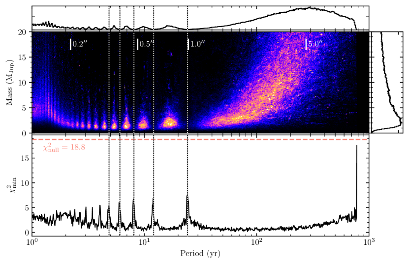
Figure 3: Period-mass posterior distribution for companions consistent with the astrometric acceleration of TW PsA measured between Hipparcos and Gaia (top panel), with associated marginalized distributions. The minimum $\chi^{2}$ as a function of period is also plotted (bottom panel), highlighting the aliasing with integer fractions of the 24.25-year baseline between the two missions (dashed vertical lines).

A two-dimensional histogram of the period and mass of companions consistent with the measured astrometry is shown in Figure 3, along with their marginalized distributions and a plot of the minimum $\chi^{2}$ as a function of orbital period. The astrometric signal is consistent with the perturbation of TW PsA by a planetary-mass companion, although the period is almost completely unconstrained. The periodic nature of the high probability regions in the mass-period plane is due to aliasing of the orbit with the 24.25-year baseline between the Hipparcos and Gaia missions. At periods greater than 25 yr the mass and period are strongly correlated; a longer period corresponds to a smaller acceleration over a 25-year baseline given a fixed mass and so a more massive companion is required to explain the observed signal.

The astrometric acceleration is also consistent with near equal mass (and thus equal brightness) companions that, for clarity, are not shown in Figure 3. The photocenter orbit induced by a near equal brightness companion mimics that of a significantly lower mass companion that contributes negligible flux. A massive stellar companion would induce a significant radial velocity signal, or would be readily identified with high-contrast imaging, depending on its orbital period. It would be surprising if such a well-studied nearby, young star had a stellar companion that had not been discovered despite numerous studies with a variety of instruments. Indeed, we strongly exclude a stellar companion to TW PsA over a wide range of orbital periods based on literature radial velocities (Section 3), and dedicated high-contrast imaging (Section 4).

2.4 Null hypothesis

The significance of the astrometric acceleration can be tested by repeating the same fit with $M_{2}$ fixed to zero and comparing the goodness of fit to that of the original model. The only free parameters in this fit are the four astrometric parameters defining the position and motion of the barycenter. We find a $\chi^{2}_{\rm min}=18.8$ for this simplified model, compared with $\chi^{2}_{\rm min}=0.05$ found previously. While the change in the $\chi^{2}_{\rm min}$ suggests that adding a massive companion significantly improves the quality of the fit, the magnitude of the change is not surprising given that the number of free parameters in the model has more than doubled. We therefore used the Bayesian information criterion (BIC) to evaluate the improvement in the quality of the fit. The BIC is defined as $\chi^{2}+k\ln n$, where $k$ is the number of parameters in the model, and $n$ is the number of data points. The BIC strongly penalizes the inclusion of additional free parameters in the model to improve the quality of the fit. The $\Delta$BIC between the two models was calculated to be $4.2$ in favour of the eleven-parameter fit, supporting the companion hypothesis but not at a significant level using the categorization from (Kass & Raftery, 1995). The penalty for having more model parameters is particularly apparent from the $\Delta$BIC calculated when considering only near-circular ($e<0.001$) orbits from the fit in Section 2.3. For this subset $e$ and $\omega$ are effectively fixed, reducing the number of free parameters to seven. We find $\chi^{2}_{\rm min}=0.5$ for this subset, corresponding to $\Delta$BIC=12.0, strong evidence in favour of the companion hypothesis in this restricted scenario.

3 Radial Velocities

TW PsA was noted by Busko & Torres (1978) as potentially being a spectroscopic binary, probably due to the range of radial velocities given for the star in the literature at the time (0–15 km s^-1; Popper, 1942; Joy, 1947; Evans et al., 1957). No individual investigator noted a variable velocity for the star, although only a handful of measurements were taken by each. Another astrophysical source of radial velocity variations is stellar jitter, a signal induced by the chromospheric activity of young, solar-type stars. TW PsA appears moderately active relative to stars of a similar age, with $\log R^{\prime}_{\rm HK}=-4.5$ to $-4.3$ (Henry et al., 1996; Gray et al., 2006; Jenkins et al., 2006). A fit to the scatter of radial velocity measurements as a function of stellar activity for a large sample of young stars demonstrates a clear trend of decreasing jitter with decreasing $\log R^{\prime}_{\rm HK}$ (Hillenbrand et al., 2015). Using this empirical relation, the measured activity index for TW PsA suggests a jitter amplitude of $\sigma_{v}=25_{-13}^{+25}$ m s^-1, several orders of magnitude smaller than the discrepancy between the historical radial velocity measurements. More modern radial velocity measurements have provided a more consistent estimate for the velocity of 7.0–7.2 km s^-1 (Chubak & Marcy, 2011; Soubiran et al., 2013; Gaia Collaboration et al., 2018), evidence against TW PsA being a spectroscopic binary.

3.1 Literature Keck/HIRES velocities

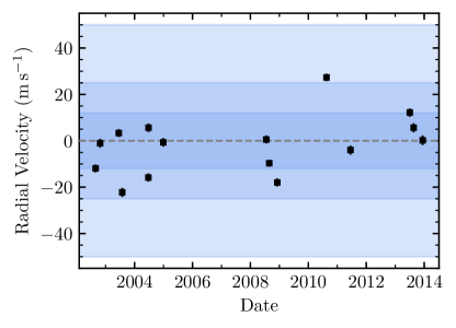
Figure 4: Radial velocity measurements of TW PsA obtained with Keck/HIRES over an eleven year baseline (Butler et al., 2017; Tal-Or et al., 2019). The weighted average of the velocities was subtracted, centering the measurements around 0 km s^-1. The amplitude of the stellar jitter estimated from activity indicators is highlighted (dark blue - 16th percentile, blue - median, light blue - 84th percentile).

Comparing radial velocities measured using different instruments and different data reduction techniques can be problematic when searching for small-amplitude velocity variations. To mitigate these potential biases, we used spectroscopic measurements of TW PsA taken over a long baseline with the same instrument and reduced and analyzed with the same pipeline. High-resolution optical echelle spectra of TW PsA were taken regularly with the HIRES instrument on the Keck I telescope as part of the Lick-Carnegie Exoplanet Survey (Butler et al., 2017). A total of fifteen radial velocity measurements of the star were made between mid-2002 and late-2013 (Figure 4). The velocities were initially published in Butler et al. (2017), but were recently corrected for small systematic errors by Tal-Or et al. (2019). While the measurement error on each individual velocity is small, there is a significant scatter about the mean. The amplitude of this scatter is consistent with the amplitude of the stellar jitter expected given the activity indicators measured for TW PsA.

The radial velocities do not exhibit large-amplitude variations induced by an orbiting stellar companion. Face-on orbits are not strictly excluded, however the inclination for a stellar companion would have to be very small. For example, a 0.1 $M_{\odot}$ companion on a circular orbit with a semi-major axis of 0.1  au requires an inclination of $i<1^{\circ}$ to induce a velocity semi-amplitude less than $30$ m s^-1. This limit rises to $i<3^{\circ}$ for a 1 au orbit, and $i<8^{\circ}$ for a 10 au orbit, wide enough to be resolved via direct imaging.

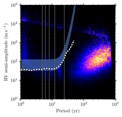
Figure 5: Period-RV semi-amplitude posterior distribution for companions consistent with the astrometric acceleration of TW PsA measured between Hipparcos and Gaia. A distinct population of stellar companions is seen with a semi-amplitude of $K_{1}>1$ km s^-1, as well as a significant population at longer periods and lower semi-amplitudes. The sensitivity of the HIRES RV record calculated using the injection recovery framework is plotted (dashed), as well as an analytical approximation using the framework described in Howard & Fulton (2016) (blue region denotes possible range of the sensitivity limit).

To assess the sensitivity of these measurements to stellar and substellar companions, we used an injection and recovery scheme written within the framework of the radvel radial velocity analysis code (Fulton et al., 2018). In brief, we simulated 10000 synthetic orbital signatures with orbital periods ranging from 10 to 20000 days and Doppler semi-amplitudes ranging from 10 m s^-1 to 100 km s^-1. These broad ranges allowed us to probe companions from the planetary to the stellar mass regime, and out to well beyond the time baseline of the RV data. For each synthetic companion, the RV curve was computed and added to the existing RV data. A least-squares minimization was then performed with period fixed near the injected period and all other parameters allowed to vary. We compared the resulting best-fit solution to a zero-companion solution via the BIC to determine whether the injected companion was recovered.

This methodology was a simplified version of a full injection and recovery test as described in Howard & Fulton (2016), since we checked the solution at only the injected period, rather than computing a full periodogram for each injected companion. We found that the small number of RV observations and sparsity of the cadence prevented traditional recovery from a full periodogram. Because of the complicated window function of the data, the periodogram structure was characterized by strong peaks at many different aliases of the injected period, which overwhelmed the true injected peak, particularly for large-amplitude injections. A real high-mass companion would therefore be evident in the periodogram structure, but would be difficult to characterize from this data alone. Because of this detail, we note that the results of our injection/recovery test likely overestimate our sensitivity to companions. However, the results, plotted in Figure 5, are useful as an estimate for the regions of parameter space in which a companion could still be located. As a conservative estimate, the RV data alone cannot rule out companions with periods $\gtrsim 40$ yr or with RV semi-amplitudes of $<30$ m s^-1.

4 Direct Imaging

TW PsA has been observed with several high-contrast imaging systems (e.g., Keck/NIRC2, Gemini South/GPI, VLT/SPHERE) that have sufficient sensitivity to detect stellar and substellar companions over a range of angular separations and masses. For example, Nielsen et al. (2019) report a null detection of substellar companions around TW PsA in their Gemini Planet Imager observations, despite having sensitivity to stellar, brown dwarf, and high-mass giant planets between $\sim 0\farcs 2$ and $1\arcsec$ radius. TW PsA is not an optimal target for instruments such as GPI that operate at near-infrared wavelengths (1–2 µm); at $\sim$450 Myr, giant planets will have cooled sufficiently such that the contrast between star and planet will be more favourable for direct detection at wavelengths between 3 µm and 5 µm.

4.1 Keck II/NIRC2 observations

TW PsA was observed on 2012 July 20 with the NIRC2 instrument on the Keck II telescope in conjunction with the facility adaptive optics (AO) system. Observations were conducted with TW PsA serving as its own AO natural guide star and the instrument in vertical angle mode, causing the angle of North to change with the parallactic angle of the target over time. This observing mode enables angular differential imaging (ADI; Marois et al., 2006), where the point-spread function remains fixed relative to the detector while astrophysical signals rotate as the target transits the observatory. Conditions were photometric with atmospheric seeing ${\sim}0\farcs 6$ and precipitable water vapor ${\sim}2$ mm. The star was placed behind the 100 mas radius semi-transparent coronagraphic mask (“corona200”), except when offset to obtain a measurement of the sky background. We obtained 49 0.8-s images with 30 coadds, the short exposure time being necessary to both prevent saturation near the edge of the coronagraphic mask and to limit the number of thermal background counts within each image. The field of view rotated by $15.6\deg$ and airmass ranged from 1.60 to 1.69 over the course of the sequence. 48 sky offset frames were obtained at the mid-point and end of the observing sequence. All observations were taken using the $L^{\prime}$ filter (3.4–4.1 µm), inscribed circle pupil, and the narrow camera with a $10\arcsec\times 10\arcsec$ field of view and 9.952 mas pixel^-1 plate scale (Yelda et al., 2010). We did not obtain any images of TW PsA where the star was not saturated. Instead, we observed the $L^{\prime}$ photometric calibrator star G158-27 ($L^{\prime}=6.898\pm 0.014$ mag) immediately afterwards, obtaining nine 0.2-s images, with 50 coadds per image, in a three-point dither pattern.

After standard bias subtraction and thermal background subtraction, we masked cosmic-ray hits and other bad pixels. We then aligned individual exposures relative to each other via cross-correlation of their stellar diffraction spikes (Marois et al., 2006) and the absolute star center was measured via radon transform (Pueyo et al., 2015). Following the procedure described in Esposito et al. (2014), we applied a LOCI algorithm (“locally optimized combination of images”; Lafrenière et al., 2007) to suppress the stellar PSF and quasistatic speckle noise in the data. The reduction presented herein used manually tuned parameters of $N_{\delta}=0.1$, $W=10$ pixels, $dr=10$ pixels, $g=0.5$, and $N_{a}=10$ to subtract the region between radii of 11 and 470 pixels, following the conventional parameter definitions in Lafrenière et al. (2007). Individual PSF-subtracted frames were then derotated to place north up and averaged to produce the final image.

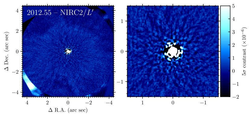
Figure 6: Sensitivity to point sources in the vicinity of TW PsA from the NIRC2 $L^{\prime}$ images after PSF subtraction and combination. The two panels show the full field of view (left) and the inner $1\farcs 5$ (right). No point source is detected at a significant level within $4\farcs 7$.

4.2 Companion mass limits

We established our sensitivity to point sources in the NIRC2 data by computing achieved contrast as a function of projected separation. To do so, we first converted the final LOCI image from detector counts to contrast units via the measured flux of the photometric calibrator star (G158-27), assuming the photometric conditions to be constant between the science and calibration observations. We then measured the azimuthally-averaged $5\sigma$-equivalent contrast limits as a function of separation from the star (Mawet et al., 2014). Finally, we corrected the contrast curves for point-source flux attenuation from LOCI PSF subtraction, which we determined by injecting and recovering simulated planets of known brightness across our separation range. The final contrast curve is shown in Figure 7.

To assess the sensitivity of these observations to planets around TW PsA, we used the Sonora grid, a combined evolutionary and atmospheric model grid for cloud-free substellar objects (Marley et al. 2019, in prep.). A mass-magnitude relationship was created for each filter by performing a linear interpolation of the atmospheric model grid at the predicted temperature and surface gravity of each point within the evolutionary grid. Fluxes at arbitrary planet mass and age could then be calculated by performing a linear interpolation of this new grid. The rapid decline in temperature for substellar objects as a function of their age results in companions $<1$ M_Jup having temperatures lower than the lowest temperature within the grid at 320 Myr, rising to $<1.5$ M_Jup at 560 Myr. For the purposes of this study, we assume that planets that do not lie within the boundary of the atmospheric grid have zero flux. For higher-mass brown dwarf and stellar companions we instead use the COND03 evolutionary models (Baraffe et al., 2003). The mass limits for a given $\Delta L^{\prime}$ from both the Sonora and COND03 evolutionary models are shown in Figure 7.

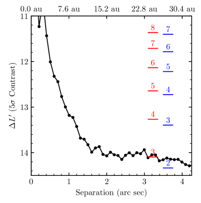
Figure 7: Azimuthally averaged $5\sigma$ contrast curve calculated from the final PSF-subtracted image of TW PsA. Companion mass limits (in $M_{\rm Jup}$) are shown, derived from the Sonora (red) and COND03 (blue) evolutionary models assuming an age of 440 Myr, and an apparent magnitude of $L^{\prime}=3.8$ mag for TW PsA. Projected separation is shown assuming a distance of 7.6 pc.

5 Joint Constraints

5.1 Revised astrometric model

The model described in Section 2.3 used to identify TW PsA as potentially hosting a substellar companion makes a simplifying assumption that Hipparcos and Gaia both measured the average proper motion of the photocenter over the duration of their respective missions. While this assumption is valid for companions on a long orbital period, where the change in proper motion over a few years is small relative to the astrometric precision, it breaks down for short-period systems that exhibit significant curvature in the photocenter orbit over a few years. For these short-period systems, the average proper motion measured by either Hipparcos or Gaia is a strong function of the phasing of the measurements with respect to the photocenter orbit, especially for eccentric systems. The model described in Section 2.3 attempts to account for this bias by performing a least-squares fit to the location of the photocenter on the dates that Hipparcos and Gaia obtained an astrometric measurement of the star. This approximation assumes that the measurements are equally weighted, and does not account for the one-dimensional nature of the measurement where the location of the star is only constrained along a given direction.

The plausible range of periods for the companion (Figure 3) motivated us to use the actual astrometric measurements made by the Hipparcos satellite to constrain the curvature of the photocenter orbit over the Hipparcos epoch. These observations, the Intermediate Astrometric Data (IAD; van Leeuwen, 2007b), are 87 one-dimensional measurements of the position of TW PsA measured by the Hipparcos satellite between 1989.96 and 1992.86. The orientation ($\psi$) of these scans relative to the celestial sphere determines how constraining each measurement is in the $\alpha^{\star}$ and $\delta$ directions, with a typical scan uncertainty of $2.8\pm 0.6$ mas. We reconstructed the original abscissa measurement using the residuals to the five-parameter fit ($\alpha^{\star}_{0}$, $\delta_{0}$, $\pi$, $\mu_{\alpha^{\star}}$, $\mu_{\delta}$) given in the IAD, and the catalogue astrometry for TW PsA from the Hipparcos re-reduction (van Leeuwen, 2007a).

The reconstructed abscissa $\Lambda_{\rm HIP}$ can be compared to a model abscissa $\Lambda_{\rm phot}$ that includes the photocenter motion induced by the orbiting companion, calculated as

$$\begin{split}\Lambda_{\rm phot}=&\left[\alpha^{\star}+t\mu_{\alpha^{\star}}+x_{\rm orbit}\left(t\right)\right]\cos\psi\\ &+\left[\delta+t\mu_{\delta}+y_{\rm orbit}\left(t\right)\right]\sin\psi\\ &+\pi\Pi\left(t\right),\end{split}$$ (3)

where $t$ are the scan epochs in years relative to 1991.25, $x_{\rm orbit}$ and $y_{\rm orbit}$ are the position of the photocenter relative to the barycenter, and $\Pi$ is the parallax factor (Sahlmann et al., 2010). Reconstructing the abscissa and performing the fit in two dimensions using the method outlined in Nielsen et al. (2019b, submitted) produces consistent results. These measurements were incorporated into the model described in Section 2.3 by replacing the first term of Equation 1 with $\chi^{2}_{\rm H}$, calculated using the reconstructed abscissa and Equation 3 as

$$\chi^{2}_{\rm H}=\left[\left(\Lambda_{\rm HIP}-\Lambda_{\rm phot}\right)/\sigma_{\Lambda_{\rm HIP}}\right]^{2}.$$ (4)

The measurements used to construct the Gaia DR2 catalogue are not due to be released until the conclusion of the nominal mission, so we are not yet able to incorporate the individual Gaia measurements into our model. The good quality of the astrometric fit relative to stars of a similar magnitude, and the lack of any significant detection of astrometric excess noise, suggests that the assumption of linear motion of the photocenter over the Gaia epoch is reasonable. A significant detection of curvature in the photocenter motion would lead to a worse $\chi^{2}$ as all stars within the catalogue were fit using the same five-parameter astrometric model. Once these individual measurements become publicly available, the analysis presented within this work should be repeated. The improvement in the precision of the astrometric measurements relative to Hipparcos will significantly constrain the mass and orbital properties of any companion to TW PsA.

5.2 RV and imaging constraints

The constraints provided by the radial velocity record (Section 3) and the high-contrast imaging dataset (Section 4) were incorporated into the model by including two additional terms when calculating the goodness of fit; $\chi^{2}_{\rm RV}$ and $\chi^{2}_{\rm Img}$. The first was calculated as

$$\chi^{2}_{\rm RV}=\sum_{i}\left(\frac{v_{i,\rm obs}-v_{i,\rm model}}{\sqrt{\sigma_{v_{i}}^{2}+\sigma_{\rm jitter}^{2}}}\right)^{2},$$ (5)

where $v_{\rm obs}$ are the HIRES radial velocities, $v_{\rm model}$ are the predicted radial velocities (a combination of the reflex motion induced by the companion at each epoch and systemic velocity $\gamma$), $\sigma_{v}$ are the uncertainties on each HIRES measurement, and $\sigma_{\rm jitter}$ is the amplitude of the radial velocity jitter. Following Howard et al. (2014), we added the following penalty term to the log likelihood to limit values of $\sigma_{\rm jitter}$

$$-\sum_{i}\ln\sqrt{2\pi\left(\sigma_{v_{i}}^{2}+\sigma_{\rm jitter}^{2}\right)}$$ (6)

The second term added to the goodness of fit, $\chi^{2}_{\rm Img}$, was calculated using the predicted angular separation of the companion at the NIRC2 epoch (2012.55), its apparent $L^{\prime}$ magnitude, and the NIRC2 contrast curve given in Section 4. We used the interpolated Sonora grid to predict the apparent $L^{\prime}$ magnitude of the companion. As the flux of substellar objects is a strong function of their age, we included the age of the system as a free parameter to marginalize over the age uncertainty. A magnitude difference $\Delta L^{\prime}$ was calculated assuming $L^{\prime}=3.8$ mag for TW PsA derived from empirical spectral type–color relations. $\chi^{2}_{\rm Img}$ was then calculated as

$$\chi^{2}_{\rm Img}=\left(\frac{10^{-0.4\Delta L^{\prime}}}{C\left(\rho\right)}\right)^{2},$$ (7)

where $C(\rho)$ is the value of the 1$\sigma$ contrast curve at the angular separation $\rho$ of the companion in 2012.55. The contrast curve was assumed to be azimuthally symmetric. The value of $C$ interior to the inner working angle and exterior to the outer working angle was fixed to $\infty$, resulting in $\chi^{2}_{\rm Img}=0$ for companions at these separations.

5.3 MCMC parameter estimation

Table 2: MCMC parameters, prior distributions, and fit intervals.

Parameter	Symbol	Unit	Prior	Prior interval
Semi-major axis	$a$	arc sec	Uniform ($\log a$)	$[0.001,10]$
Inclination	$i$	rad	Uniform ($\cos i$)	$[0,\pi]$
Eccentricity	$e$	$\cdots$	Uniform	$[0,1)$
Argument of periapse	$\omega$	rad	Uniform	$[0,2\pi)$
Longitude of ascending node	$\Omega$	rad	Uniform	$[0,2\pi)$
Mean anomaly at epoch	$\tau$	$\cdots$	Uniform	$[0,1)$
Companion mass	$M_{2}$	$M_{\odot}$	Uniform ($\log M_{2}$)	$[10^{-4},M_{1}]$
Systemic velocity	$\gamma$	km s-1	Uniform	$[-100,100]$
RV jitter	$\sigma_{\rm jitter}$	km s-1	$\log\sigma_{\rm jitter}\sim\mathcal{N}(-1.6,0.3^{2})$	$(0,1]$
Age	$t_{\rm age}$	Myr	$\mathcal{N}(440,40^{2})$	[100, 780]
R.A. offset at 1991.25	$\Delta\alpha^{\star}$	mas	Uniform	$[-50,50]$
Dec. offset at 1991.25	$\Delta\delta$	mas	Uniform	$[-50,50]$
Parallax	$\pi$	mas	Uniform	$(0,1000]$
System R.A. proper motion	$\mu_{\alpha^{\star}}$	mas yr-1	Uniform	$[281,381]$
System Dec. proper motion	$\mu_{\delta}$	mas yr-1	Uniform	$[-209,-109]$

This revised astrometric model included fifteen free parameters; the eleven outlined in Section 2.3, the parallax $\pi$, the systemic radial velocity $\gamma$, the amplitude of the radial velocity jitter $\sigma_{\rm jitter}$, and the age of the system $t_{\rm age}$. As in Section 2.3, we used emcee to sample the posterior distribution of these fifteen parameters. Table 2 lists the parameters, the assumed prior distribution, and the interval over which the posterior distribution was estimated. Although the prior on the RV jitter parameter was a normal distribution in $\log\sigma_{\rm jitter}$ based on the estimate for the RV jitter given in Section 3 ($\log\sigma_{\rm jitter}=-1.6\pm 0.3$ [km s^-1]; Hillenbrand et al., 2015), we fit for $\sigma_{\rm jitter}$, enforcing a log-normal prior on the parameter. The only difference in choice of priors between this and the previous fit was for the secondary mass. In Section 2.3 we used a uniform prior for $M_{2}$ where $dp/dM_{2}\propto 1$. Given that the distribution of masses for the wide-orbit giant planet population is more consistent with a power law distribution (e.g., Nielsen et al., 2019), we instead adopt a uniform prior in the logarithm of the companion mass, $dp/d\log M_{2}\propto 1$ to better match the observed distribution. The prior on the age of the system was a normal distribution using the age estimate of $440\pm 40$ Myr from Mamajek (2012).

Figure 8: As Figure 3 but for the model described in Section 5.3 that incorporates the Hipparcos IAD, the radial velocity record, and the Keck/NIRC2 contrast curves. The plausible range of companion properties has been significantly reduced relative to the initial fit shown in Figure 3; the radial velocity record has excluded short-period stellar companions, while the NIRC2 imaging data has excluded substellar companions down to $\sim$3 M_Jup beyond an arcsecond. The fit favors

a long-period ($\gtrsim$3 yr) Jovian-mass ($M_{2}=1.2_{-0.6}^{+0.7}$ M_Jup) companion.

We initialized 1024 walkers throughout parameter space at each of 20 temperatures, yielding a total of 20480 chains. Each chain was advanced for $10^{6}$ steps, and the positions were saved every hundredth step. The first half of each chain was discarded as a “burn-in”. At each step, the log likelihood $\ln\mathcal{L}$ was calculated as

$$\begin{split}\ln\mathcal{L}=&-\frac{1}{2}\left(\chi^{2}_{\rm H}+R_{\rm G}^{\top}{\mathbf{G}}_{\rm G}^{-1}R_{\rm G}+\chi^{2}_{\rm RV}+\chi^{2}_{\rm Img}\right)\\ &-\sum\ln\sqrt{2\pi\left(\sigma_{v}^{2}+\sigma_{\rm jitter}^{2}\right)}.\end{split}$$ (8)

We measured auto-correlation lengths close to unity for each parameter in the decimated chains, suggesting that each saved sample was independent from the previous sample. The median and $1\sigma$ range for each parameter did not significantly change in the remaining half of the chains. The covariance between companion period and mass after marginalizing over the remaining thirteen parameters, and corresponding 1-d marginalized distributions, are shown in Figure 8. Relative to the fit that only includes the absolute astrometry for TW PsA (Figure 3), the allowed range of parameter space has been significantly constrained. Massive ($\gtrsim$5 M_Jup) companions are excluded at short periods by the radial velocity record, and at long periods by the deep NIRC2 imaging data. Furthermore, lower-mass companions with periods shorter than $\sim$2 yrs are excluded by the radial velocity record. We find a tight constraint on the companion mass $M_{2}=1.2_{-0.6}^{+0.7}$ M_Jup, with a 1, 2, and 3$\sigma$ lower limits of 0.9, 0.2, and 0.1 M_Jup and upper limits of 1.5, 2.4, and 4.5 M_Jup. The period is less well constrained ($P=25_{-21}^{+52}$ yr), with a multi-modal posterior distribution caused by aliasing of the orbit with the 24.25-year baseline between the Hipparcos and Gaia missions.

5.4 Null hypothesis

We repeated the same exercise described in Section 2.4 where the companion mass is fixed to zero, and the only parameters that are fit are the five astrometric parameters describing the position and motion of the system barycenter ($\Delta\alpha^{\star}$, $\Delta\delta$, $\pi$, $\mu_{\alpha^{\star}}$, $\mu_{\delta}$) and the two parameters describing its radial velocity ($\gamma$, $\sigma_{\rm jitter}$). We used the same MCMC framework described in the previous subsection. We advanced 1024 walkers at each of 20 temperatures for $10^{6}$ steps, using the likelihood given in Equation 8 and the relevant priors given in Table 2. The best fit model had $\chi_{\rm null}^{2}=119.9$, compared with $\chi^{2}=101.5$ for the model including a massive companion. We calculated the BIC for the model including a massive companion (${\rm BIC}=171.6$, $k=15$, $n=107$) and the model without (${\rm BIC}_{\rm null}=152.6$, $k=7$, $n=107$). The $\Delta{\rm BIC}$ of 19.0 corresponds to very strong evidence against the companion hypothesis using the categorization from Kass & Raftery (1995), despite the significant reduction in $\chi^{2}$. The large number of measurements included in the fit leads to a very strong penalty term for each additional parameter used in the model, several of which are effectively nuisance parameters that are marginalized over.

The $\Delta$BIC suggests that the current astrometric measurements are not sufficiently constraining to justify the use of the model described in this section that incorporates a massive orbiting companion over one that assumes linear motion of the star in the sky plane. While there was evidence against the null hypothesis when using this test for the model described in Section 2.4, the addition of the 87 measurements from the Hipparcos IAD significantly increased the magnitude of the penalty term in the BIC from 2.1 to 4.7 per additional parameter. Consequently, a significantly smaller $\chi^{2}$ from the massive companion model in this section is required for there to be significant evidence against the null hypothesis here. A more precise measurement of the astrometric acceleration with future Gaia data releases will be required in order to reject the null hypothesis at a significant level using the BIC.

6 Future Prospects for Direct Detection

The range of orbital periods that satisfy the joint constraints described in the previous section correspond to angular separations ($0\farcs 2$–$5\arcsec$) at which the planet could be resolved with current and/or future ground and space-based instrumentation. Two such examples are the Near-Infrared Camera (NIRCam; Horner & Rieke, 2004) on the James Webb Space Telescope (JWST), and the visible light coronagraphic instrument (CGI; Noecker et al., 2016) on the Wide Field Infrared Survey Telescope (WFIRST). These two instruments are highly complementary. NIRCam is sensitive to thermal emission from the planet, whilst CGI is sensitive to visible light from the host star reflected off the top of the planet’s atmosphere. The youth and proximity of TW PsA, and the evidence presented here suggestive of an orbiting giant planet at a relatively wide angular separation, make it a choice target for these two missions.

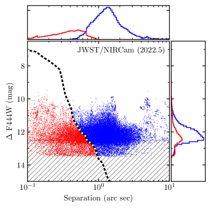
Figure 9: Predicted contrast in NIRCam’s F444W bandpass as a function of angular separation in 2022.5 for draws from the posterior distributions described in Section 5.3 that lie within the bounds of the Sonora grid. Companions that lie above the predicted NIRCam contrast curve (dashed) are plotted in blue, whereas those that are not detectable are plotted in red. The hatched region indicates contrasts at which some planets are beyond the range of the Sonora evolutionary and/or atmospheric grids. Marginalized distributions for the detectable and non-detectable samples are also plotted.

We used the Sonora model grid described previously to predict the flux of the planet in the F444W bandpass, one of the standard filters that will be used in conjunction with coronagraphic imaging with JWST. We computed the projected separation at 2022.5 for each sample within the MCMC chains from Section 5.3, and used the corresponding companion mass and system age to predict the flux in the F444W bandpass. We assumed an apparent F444W magnitude for TW PsA of 3.8 based on color transformations computed for main sequence stars. The magnitude difference between star and planet are plotted as a function of angular separation at 2022.5 in Figure 9. We find that 24 % of the draws from the posterior distributions lie above the predicted contrast of NIRCam (Beichman et al., 2010). A significant fraction (68 %) of the MCMC samples were for masses and ages that fell outside of the Sonora evolutionary and/or atmospheric grids, typically due to the predicted temperature for the planet being beyond the range of the atmospheric grid. We cannot assess their detectability with the current model grid, but a small subset at the widest angular separations will lie above the predicted contrast curve unless a significant decrease in flux at 4.5 $\micron$ occurs at temperatures below 200 K.

The proximity of TW PsA (7.6 pc) and the small angular separation make this target particularly favourable for the direct detection of the reflected light of the host star from the top of the planet’s atmosphere. We used a grid of reflectance spectra for giant planets (Batalha et al., 2018) to predict the contrast between the star and planet at 575 and 825 nm, two of the filters proposed for the CGI instrument. Within this model grid the reflectivity is expressed as the geometric albedo $p$ scaled by the phase function $\Phi$ at a given orbital phase angle $\beta$, and depends on the planet metallicity $[M/H]$, separation $r$, cloud sedimentation parameter $f_{\rm sed}$ (Ackerman & Marley, 2001), and the wavelength of the observations. We calculated orbital separations and phase angles at 2027.0 for each MCMC sample, and estimated radii using an empirical mass-radius relationship (Chen & Kipping, 2017). As the metallicity and cloud properties of the planet are not known, we calculate star to planet contrasts at each grid point within the ($[M/H]$, $f_{\rm sed}$) plane to evaluate detectability over a representative range of planet properties. The contrast and angular separation at 2027.0 was then compared to predicted CGI sensitivity curves at 575 and 825 nm assuming 100 hr of on-source integration (Nemati et al., 2017). We note that the mass-radius relationship and the reflectence model are not coupled; the radius of a solar composition planet of a given mass is assumed to be the same as one with an enhanced abundance. In reality, these higher metallicity planets would have smaller radii, and our model overestimates their detectibility.

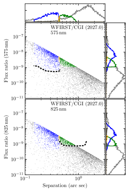
Figure 10: Reflected light contrast at 575 nm (top panel) and 825 nm (bottom panel) as a function of angular separation in 2027 for draws from the posterior distributions described in Section 5.3. Planets detectable in 100 hr with the 575 nm filter (blue), the 825 nm filter (green), or with both filters (yellow) are highlighted. Predicted sensitivity curves for imaging observations with WFIRST/CGI are overplotted (dashed lines), limited by angular size of the control region of the deformable mirror in the focal plane. Corresponding marginalized distributions are also shown.

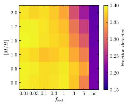
Figure 11: Fraction of planets from the MCMC posterior distributions that are detectable with WFIRST/CGI as a function of the cloud sedimentation parameter $f_{\rm sed}$ and metallicity $[M/H]$. Detection limits calculated assuming 100 hr exposure time per filter.

The predicted contrast as a function of angular separation in 2027.0 is shown for the 575 nm and 825 nm filters in Figure 10 assuming $[M/H]=0$ and $f_{\rm sed}=6$ (thin clouds), a median scenario in terms of planet detectability. The strong dependence of the planetary albedo on the cloud sedimentation parameter, and to a lesser extent the metallicity, leads to a large variation in the probability of detection as a function of these parameters (Figure 11). With efficient sedimentation (large values of $f_{\rm sed}$) the clouds are vertically thin, resulting in a relatively low albedo. As $f_{\rm sed}$ is decreased the clouds become thicker, resulting in a higher albedo. Low values for this sedimentation parameter have been required to explain observations of the atmospheres of transiting hot Jupiters (e.g., Demory et al., 2013), whereas more widely separated gas giants like Jupiter might be limited to $f_{\rm sed}\geq 3$ (Batalha et al., 2018). Assuming a solar metallicity, going from the cloud-free albedo spectra to one with thin clouds ($f_{\rm sed}=6$) increases the fraction of planets that are detectable with CGI from 20 % to 29 % due to the significant increase in the geometric albedo.

7 Conclusions

We have presented the first constraints on planetary-mass companions to the nearby (7.6 pc) young ($\sim$440 Myr) K4Ve star TW Piscis Austrini, a wide common proper motion companion to Fomalhaut, that combine absolute astrometry, direct imaging, and radial velocities. Previous studies had identified this star as exhibiting an astrometric acceleration between the Hipparcos and Gaia missions (Kervella et al., 2019). While the significance of the acceleration is $\leq 4\sigma$ in each pair of derived proper motions, the goodness of fit of the measurements to an astrometric model describing the motion of the star across the sky is significantly worse without accounting for the reflex motion induced by a massive orbiting companion. We combined these absolute astrometric measurements with Keck/NIRC2 $L^{\prime}$ coronagraphic imaging and an 11-year radial velocity record (Tal-Or et al., 2019; Butler et al., 2017) that exclude massive ($\gtrsim 5$ M_Jup $3\sigma$ limit) companions over all plausible orbital periods. The combination of this upper limit with a lower limit derived from the significant astrometric acceleration leads to a tight constraint on the mass of a companion consistent with the magnitude and direction of the acceleration of $M_{2}=1.2_{-0.6}^{+0.7}$ M_Jup. The orbital period is less constrained ($P=25_{-21}^{+52}$ yr), and is aliased with the 24.25-year baseline between the Hipparcos and Gaia missions. Continued radial velocity monitoring and deep imaging observations will further constrain the properties of this putative companion, while the upcoming Gaia data releases will more precisely measure the acceleration of the host star.

Searches for exoplanets via absolute astrometry using ground-based instrumentation have yielded either null results or candidates that were later found to be spurious (e.g., 61 Cygni, Strand, 1943; Wittenmyer et al., 2006; Van Biesbroeck’s star, Pravdo & Shaklan, 2009; Lazorenko et al., 2011). Such surveys are limited by the astrometric precision of the individual measurements, typically $>0.1$ mas (Lazorenko et al., 2009). There have also been numerous attempts to measure the astrometric signal of known exoplanets with the Fine Guidance Sensors on the Hubble Space Telescope (e.g., Benedict et al., 2017); however, several of these measurements were later found to be inconsistent with analyses incorporating additional radial velocity data (e.g., Rivera et al., 2010; Mawet et al., 2019). The exquisite precision of Gaia, an order of magnitude better than current ground-based instrumentation, is set to transform this field of study with thousands of exoplanets detected via astrometry alone (Perryman et al., 2014), the first since the discovery of Neptune in the mid-19th century.

References

- Ackerman & Marley (2001) Ackerman, A. S., & Marley, M. S. 2001, Astrophys. J., 556, 872
- Baraffe et al. (2003) Baraffe, I., Chabrier, G., Barman, T. S., Allard, F., & Hauschildt, P. H. 2003, A&A, 402, 701
- Batalha et al. (2018) Batalha, N. E., Smith, A. J. R. W., Lewis, N. K., et al. 2018, AJ, 156, 158
- Beichman et al. (2010) Beichman, C. A., Krist, J., Trauger, J. T., et al. 2010, PASP, 122, 162
- Benedict et al. (2017) Benedict, G. F., McArthur, B. E., Nelan, E. P., & Harrison, T. E. 2017, PASP, 129, 012001
- Blunt et al. (2017) Blunt, S., Nielsen, E. L., De Rosa, R. J., et al. 2017, AJ, 153, 229
- Blunt et al. (2019) Blunt, S., Wang, J., Angelo, I., et al. 2019, eprint arXiv:1910.01756
- Brandt (2018) Brandt, T. D. 2018, ApJS, 239, 31
- Busko & Torres (1978) Busko, I. C., & Torres, C. A. O. 1978, A&A, 64, 153
- Butkevich & Lindegren (2014) Butkevich, A. G., & Lindegren, L. 2014, A&A, 570, A62
- Butler et al. (2017) Butler, R. P., Vogt, S. S., Laughlin, G., et al. 2017, AJ, 153, 208
- Carpenter et al. (2008) Carpenter, J. M., Bouwman, J., Silverstone, M. D., et al. 2008, ApJS, 179, 423
- Chen & Kipping (2017) Chen, J., & Kipping, D. 2017, Astrophys. J., 834, 17
- Chubak & Marcy (2011) Chubak, C., & Marcy, G. 2011, Bulletin of the American Astronomical Society, 43
- Demory et al. (2009) Demory, B. O., Segransan, D., Forveille, T., et al. 2009, A&A, 505, 205
- Demory et al. (2013) Demory, B.-O., de Wit, J., Lewis, N., et al. 2013, ApJ, 776, L25
- Durkan et al. (2016) Durkan, S., Janson, M., & Carson, J. C. 2016, ApJ, 824, 58
- Earl & Deem (2005) Earl, D. J., & Deem, M. W. 2005, Physical Chemistry Chemical Physics (Incorporating Faraday Transactions), 7, 3910
- ESA (1997) ESA. 1997, The Hipparcos and Tycho Catalogues, ESA SP-1200
- Esposito et al. (2014) Esposito, T. M., Fitzgerald, M. P., Graham, J. R., & Kalas, P. 2014, Astrophys. J., 780, 25
- Evans et al. (1957) Evans, D. S., Menzies, A., & Stoy, R. H. 1957, MNRAS, 117, 534
- Foreman-Mackey et al. (2013) Foreman-Mackey, D., Hogg, D. W., Lang, D., & Goodman, J. 2013, PASP, 125, 306
- Fulton et al. (2018) Fulton, B. J., Petigura, E. A., Blunt, S., & Sinukoff, E. 2018, PASP, 130, 044504
- Gaia Collaboration et al. (2018) Gaia Collaboration, Brown, A. G. A., Vallenari, A., et al. 2018, A&A, 616, A1
- Gray et al. (2006) Gray, R. O., Corbally, C. J., Garrison, R. F., et al. 2006, AJ, 132, 161
- Heinze et al. (2010) Heinze, A. N., Hinz, P. M., Sivanandam, S., et al. 2010, Astrophys. J., 714, 1551
- Henry et al. (1996) Henry, T. J., Soderblom, D. R., Donahue, R. A., & Baliunas, S. L. 1996, AJ, 111, 439
- Hillenbrand et al. (2015) Hillenbrand, L., Isaacson, H., Marcy, G., et al. 2015, 18th Cambridge Workshop on Cool Stars, Stellar Systems, and the Sun, 759
- Holland et al. (1998) Holland, W. S., Greaves, J. S., Zuckerman, B., et al. 1998, Nature, 392, 788
- Horner & Rieke (2004) Horner, S. D., & Rieke, M. J. 2004, Ground-based and Airborne Instrumentation for Astronomy VI, 5487, 628
- Howard & Fulton (2016) Howard, A. W., & Fulton, B. J. 2016, PASP, 128, 114401
- Howard et al. (2014) Howard, A. W., Marcy, G. W., Fischer, D. A., et al. 2014, Astrophys. J., 794, 51
- Hunter (2007) Hunter, J. D. 2007, Comput. Sci. Eng., 9, 90
- Jenkins et al. (2006) Jenkins, J. S., Jones, H. R. A., Tinney, C. G., et al. 2006, MNRAS, 372, 163
- Joy (1947) Joy, A. H. 1947, Astrophys. J., 105, 96
- Kalas et al. (2008) Kalas, P., Graham, J. R., Chiang, E., et al. 2008, Science, 322, 1345
- Kass & Raftery (1995) Kass, R. E., & Raftery, A. E. 1995, Journal of the American Statistical Association, 90, 773
- Keenan & McNeil (1989) Keenan, P. C., & McNeil, R. C. 1989, ApJS, 71, 245
- Kennedy et al. (2014) Kennedy, G. M., Wyatt, M. C., Kalas, P., et al. 2014, Monthly Notices of the Royal Astronomical Society: Letters, 438, L96
- Kervella et al. (2019) Kervella, P., Arenou, F., Mignard, F., & Thévenin, F. 2019, A&A, 623, A72
- Lafrenière et al. (2007) Lafrenière, D., Marois, C., Doyon, R., Nadeau, D., & Artigau, É. 2007, ApJ, 660, 770
- Lazorenko et al. (2009) Lazorenko, P. F., Mayor, M., Dominik, M., et al. 2009, A&A, 505, 903
- Lazorenko et al. (2011) Lazorenko, P. F., Sahlmann, J., Segransan, D., et al. 2011, A&A, 527, A25
- Lindegren et al. (2018) Lindegren, L., Hernández, J., Bombrun, A., et al. 2018, A&A, 616, A2
- Luyten (1938) Luyten, W. J. 1938, AJ, 47, 115
- Mamajek (2012) Mamajek, E. E. 2012, Astrophys. J., 754, L20
- Mamajek et al. (2013) Mamajek, E. E., Bartlett, J. L., Seifahrt, A., et al. 2013, AJ, 146, 154
- Marois et al. (2006) Marois, C., Lafrenière, D., Doyon, R., Macintosh, B., & Nadeau, D. 2006, ApJ, 641, 556
- Mawet et al. (2014) Mawet, D., Milli, J., Wahhaj, Z., et al. 2014, Astrophys. J., 792, 97
- Mawet et al. (2019) Mawet, D., Hirsch, L., Lee, E. J., et al. 2019, VizieR Online Data Catalog, 157, 33
- Michalik et al. (2014) Michalik, D., Lindegren, L., Hobbs, D., & Lammers, U. 2014, A&A, 571, A85
- Nemati et al. (2017) Nemati, B., Krist, J. E., & Mennesson, B. 2017, in Techniques and Instrumentation for Detection of Exoplanets VIII, ed. S. Shaklan (SPIE), 7
- Nielsen et al. (2019) Nielsen, E. L., De Rosa, R. J., Macintosh, B., et al. 2019, eprint arXiv:1904.05358
- Noecker et al. (2016) Noecker, M. C., Zhao, F., Demers, R., et al. 2016, J. Astron. Telesc. Instrum. Syst., 2, 011001
- Pecaut & Mamajek (2013) Pecaut, M. J., & Mamajek, E. E. 2013, ApJS, 208, 9
- Perryman et al. (2014) Perryman, M., Hartman, J., Bakos, G. Á., & Lindegren, L. 2014, ApJ, 797, 14
- Popper (1942) Popper, D. M. 1942, Astrophys. J., 95, 307
- Pravdo & Shaklan (2009) Pravdo, S. H., & Shaklan, S. B. 2009, Astrophys. J., 700, 623
- Pueyo et al. (2015) Pueyo, L., Soummer, R., Hoffmann, J., et al. 2015, ApJ, 803, 31
- Rivera et al. (2010) Rivera, E. J., Laughlin, G., Butler, R. P., et al. 2010, Astrophys. J., 719, 890
- Sahlmann et al. (2014) Sahlmann, J., Lazorenko, P. F., Segransan, D., et al. 2014, A&A, 565, A20
- Sahlmann et al. (2010) Sahlmann, J., Segransan, D., Queloz, D., et al. 2010, A&A, 525, A95
- Shannon et al. (2014) Shannon, A., Clarke, C., & Wyatt, M. 2014, MNRAS, 442, 142
- Shaya & Olling (2010) Shaya, E. J., & Olling, R. P. 2010, ApJS, 192, 2
- Soubiran et al. (2013) Soubiran, C., Jasniewicz, G., Chemin, L., et al. 2013, A&A, 552, A64
- Strand (1943) Strand, K. A. 1943, PASP, 55, 29
- Tal-Or et al. (2019) Tal-Or, L., Trifonov, T., Zucker, S., Mazeh, T., & Zechmeister, M. 2019, MNRAS, 484, L8
- The Astropy Collaboration et al. (2013) The Astropy Collaboration, Robitaille, T. P., Tollerud, E. J., et al. 2013, A&A, 558, A33
- van Leeuwen (2007a) van Leeuwen, F. 2007a, A&A, 474, 653
- van Leeuwen (2007b) —. 2007b, Astrophysics and Space Science Library, 350
- Wittenmyer et al. (2006) Wittenmyer, R. A., Endl, M., Cochran, W. D., et al. 2006, AJ, 132, 177
- Yelda et al. (2010) Yelda, S., Lu, J. R., Ghez, A. M., et al. 2010, ApJ, 725, 331