ZMCintegral-v5: Support for Integrations with the Scanning of Large Parameter Grids on Multi-GPUs

Abstract

In this updated vesion of ZMCintegral, we have added the functionality of integrations with parameter scan on distributed Graphics Processing Units(GPUs). Given a large parameter grid (up to $10^{10}$ parameter points to be scanned), the code will evaluate integrations for each parameter grid value. To ensure the evaluation speed, this new functionality employs a direct Monte Carlo method for the integraion. The Python API is kept the same as the previous ones and users have a full flexibility to define their own integrands. The performance of this new functionality is tested for both one node and multi-nodes conditions.

PROGRAM SUMMARY

Manuscript Title: ZMCintegral-v5: Support for Integrations with the Scanning of Large Parameter Grids on Multi-GPUs
Authors: Jun-Jie Zhang;Hong-Zhong Wu
Program Title: ZMCintegral
Journal Reference:
Catalogue identifier:
Licensing provisions: Apache License Version, 2.0(Apache-2.0)
Programming language: Python
Operating system: Linux
Keywords: Grid parameter search;parameter scan;Numba; Ray; Monte Carlo integration.
Classification: 4.12 Other Numerical Methods
External routines/libraries: Numba; Ray;
Nature of problem: Easy to use python package for integrations with large parameter grids using Monte Carlo method on distributed GPU clusters.
Solution method: Direct Monte Carlo method and distributed computing.

1 Introduction

In the real application of ZMCintegral, we find that for many cases users usually have integrations with various parameters. The previous versions[1] of our package mainly fouces on high dimensional integration, and lack the performance for a search of the parameter grids. Furthermore, there are many ereas that require the integration involving parameters while the dimensionality is not very high. For example, the solving of GAP equations in finite temperature field[2, 3], the branching fractions predictions in meson decay[4], the solving of transport equations in phase space for quark gluon plasma[5, 6, 7], the calculation of global polarization at different coherent length in heavy iron collisions[8], etc. Therefore, we add this new functionality of parameter grid search to version-5. In fact, there have been many packages[9, 10, 11, 12] (for specific use), and also commercial softwares (Mathematica, Matlab, etc.) that have good performance for parameter grid search with CPU devices. Also, with the development of GPU CUDA[13], integrations on CUDA for decoupled ODEs (ordinary differential equations) with various initial conditions (can be seen as parameters), has also been developed[14].

For our scheme, we mainly work on a general-use Python package with Monte Carlo integration on multi-GPUs of distributted clusters. In this updated version, we have added the functionality where users can provide a large series of parameters for the integration, and the package requires Numba[15] and Ray[16] to be pre-installed. Since this functionality is mainly for the search of the parameter grid, we have merely applied the direct (or simple) Monte Carlo method[17] without stratified sampling and heuristic tree search to ensure the speed performance. The source codes and manual can be found in Ref. [18]. The Python API is kept the same as the previous ones and users have a full flexibility to define their own integrands.

In this paper, we first introduce the general structure of the functionality of this new version. Then, few examples have been introduced to demonstrate the performance of the speed and accuracy. For users who have a large parameter grid (up to $10^{10}$ parameter grid points), this new functionality (version-5) will be suitable.

2 Integration with parameter grid

In our code, the general form of the integration with parameters is defined as

$$f(\mathbf{x}) = \int\text{$d\mathbf{y}$}g(\mathbf{y};\mathbf{x}),$$ (1)

where vector $\mathbf{y}=(y_{1},\cdots y_{N})$ is the integration variable, $\int\text{$d\mathbf{y}$}\equiv\int\prod_{k=1}^{N}dy_{k}$, and vector $\mathbf{x}=(x_{1},\cdots x_{M})$ is the grid point of the parameter grid. Each parameter $x_{i}$ in $\mathbf{x}=(x_{1},\cdots x_{M})$ takes values from a list, which contains the values that need to be scanned for this specific parameter $x_{i}$.

With any given $\mathbf{x}$, the integration will be evaluated using the direct Monte Carlo method. Currently, it is time consuming to perform a stratified sampling with large parameter grids. Hence, to increase speed, we only consider the application of a direct MC, and limit the usage for this version to large parameter grid and small dimensional integration . For higher dimensional integration with small parameter grid , the previous versions[1] can take the role.

The same as the previous versions, we haved used the package Ray[16] and Numba[15] to perform multi-GPU calculations on distributed clusters. The returned result is a multi-dimensional grid with each element being the integrated values.

In the real calculation, we cut the parameter grid into several batches. Each batch is fed into one GPU device for evaluation. A task can either be assigned sequentially to one GPU or parallelly to several distributed GPUs. The integration is performed on every GPU thread, hence, each thread gives the integration value of one parameter. This porcess is shown in Fig. 1.

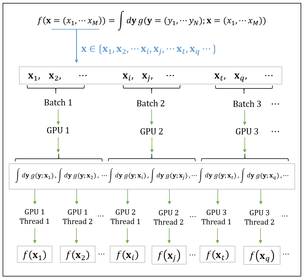
Figure 1: Schematic diagram of distributed GPU evaluation. Given the parameter grid value $\mathbf{x}_{1},\mathbf{x}_{2}\cdots$, the corresponding integrations $\int d\mathbf{y}g(\mathbf{y};\mathbf{x}_{1})$, $\int d\mathbf{y}g(\mathbf{y};\mathbf{x}_{1})\cdots$ can be evaluated in different GPU threads via direct Monte Carlo method. In our algorithm, each batch is assigned to one GPU and each integration is assigned to one thread.

3 Results and performance

3.1 Test on one node

The hardware condition for this node is Intel(R) Xeon(R) Silver 4110 CPU@2.10GHz CPU with 10 processors + 1 Nvidia Tesla V100 GPU.

We test our code with an oscillating integrand

$$f(x_{1},x_{2},\cdots x_{M}) = (\prod_{k=1}^{N}\int_{0}^{10}dy_{k})\text{sin}(\sum_{j}^{N}y_{j}+\sum_{l=1}^{M}x_{l}),$$ (2)

where $N$ is the dimension of the integrations. Each parameter $x_{i}$ in $\mathbf{x}=(x_{1},\cdots x_{M})$ takes values from the list $\{0,1,2,\cdots 99\}$, which contains the values that need to be scanned for this specific parameter $x_{i}$. Therefore, the parameter grid has $100^{M}$ points. Hence we need to scan over $100^{M}$ points, with each point containing an integration of $N$ dimensions.

Here we choose $M\in\{1,2,3,4\}$ and $N\in\{1,2,3,4\}$to see the time consumption of HToD(host to device), DToH(device to host) and the total evaluation. Since the theoretical value of this integration can be obtained directly, we also compare our results with the theoretical ones. We introduce the relative error $\delta r$ as

$$\delta r \equiv \frac{1}{100^{M}}\sum_{i=1}^{100^{M}}\frac{|f_{\text{theoretical}}^{i}-f_{\text{ZMC}}^{i}|}{f_{\text{theoretical}}^{i}}.$$ (3)

Tab. 1 and Fig. 2 show the results of the performance of our code on one node. We can see from the upper-left part of Fig. 2 that for a large parameter scan, the dimension of the integration should not be very large. In our case, we have chosen an oscillating function and used merely $10^{4}$ sample points for each integration. Therefore, we obtain a large error for dimension $N=4$. However, in real ceses one can use more sample points (e.g. $\geq 10^{4}$) for higher dimensinal integrations (e.g. $N\geq 4$, see Sec. 3.2). Since the parameter grid has $100^{M}$ points, with the increase of $M$, the parameter grid size increases exponentially. This exponential increase explains the close gap between $M=1,2,3$, and a large gap between $M=4$ and $M=1,2,3$ in Fig. 2.

Table 1: Performance for oscillating integrands on one node. This node contains one V100 GPU. $M\in\{1,2,3,4\}$ and $N\in\{1,2,3,4\}$ stand for the number of parameters and the dimension of the integration respectively. The integration is performed via the direct Monte Carlo method with 10000 samples. Number of batches is set to 1. The data is plotted in Fig. 2.

$(M,N)$	$(1,1)$	$(1,2)$	$(1,3)$	$(1,4)$	$(2,1)$	$(2,2)$	$(2,3)$	$(2,4)$
$\delta r$	0.02512	0.25034	1.19949	6.19901	0.03379	0.16417	0.87280	4.12216
HToD (ms)	0.72227	0.84085	0.70653	0.96030	1.14849	1.01440	1.19109	1.13764
DToH (s)	0.00010	0.00011	0.00010	0.00010	0.00012	0.00013	0.00012	0.00013
total time (s)	0.59343	0.57227	0.59330	0.60408	0.61858	0.59581	0.61055	0.62169
$(M,N)$	$(3,1)$	$(3,2)$	$(3,3)$	$(3,4)$	$(4,1)$	$(4,2)$	$(4,3)$	$(4,4)$
$\delta r$	0.02927	0.15052	0.78052	4.05029	0.08806	0.55222	3.55857	22.62904
HToD (ms)	1.23856	1.19336	1.37538	1.41807	2.79922	2.68347	2.77383	2.64370
DToH (s)	0.00200	0.00303	0.00197	0.00268	0.60880	0.61748	0.59681	0.59422
total time (s)	1.26269	1.51221	1.78097	2.07094	64.8745	91.5998	118.275	147.347

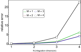
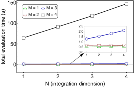
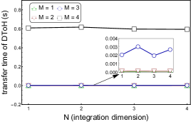
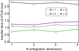
Figure 2: Performance for oscillating integrands on one node. This node contains one Nvidia Tesla V100 GPU. The upper-left panel demonstrates the calculation error (defined in Eq. (3)) in terms of $M$ and $N$. It can be seen that with the increase of the dimensions, the relative error increases really fast. The upper-right panel shows the total evaluation time of Eq. (2). We can see that the total time increases with the increase of both $M$ and $N$. The lower panel dimenstrates the transfer time of DToH (device to host) and HToD (host to device). This transfer time mainly depends on the size of the parameter grid, i.e. $M$, and is not sensitive to the integration dimension $N$.

3.2 Test on multipole nodes

We use totally three nodes in this section. The hardware condition for the three nodes are Intel(R) Xeon(R) CPU E5-2620 v3@2.40GHz CPU with 24 processors + 4 Nvidia Tesla K40m GPUs, Intel(R) Xeon(R) CPU E5-2680 V4@2.40GHz CPU with 10 processors + 2 Nvidia Tesla K80 GPUs, and Intel(R) Xeon(R) Silver 4110 CPU@2.10GHz CPU with 10 processors + 1 Nvidia Tesla V100 GPU. The K80 card can be seen as the combination of two K40 cards in physical structure. These three nodes are in a local area network.

Different from integrating one single function, where most computational resources can be used to generate sample points, the parameter grid search deals with millions of integrands of different parameters. Therefore, the computational resources are used to loop thorugh the parameters. As is introduced in Sec. 2, a single thread needs to generate all sample points to perform the integration of a certain parameter point. This means that the sample points for each thread can not be very large. For this parameter scan functionality, we suggest a number of sample points not exceed $10^{6}$ (for grid size ~ $10^{8}$) for one Tesla V100 (this configuration will take roughly 6 hours with Intel(R) Xeon(R) Silver 4110 CPU@2.10GHz CPU with 10 processors + 1 Nvidia Tesla V100 GPU). However, for users with large GPU clusters, this number can be set higher. Since we adopt the direct Monte Carlo method to implement the integration, the accuracy of the integration only depends on the number of sample points. In the real application, users need to firstly determine the number of sample points based on the desired accuracy. Then start with some small value for the sample number, and increase this value to see if the evaluation time is acceptable.

Now we test the performance of the code on three nodes with the integrand

$$f(x_{1},x_{2},x_{3},x_{4}) = (\prod_{k=1}^{6}\int_{0}^{1}dy_{k})\text{sin}(\sum_{j}^{6}y_{j}+\sum_{l=1}^{4}x_{l}),$$ (4)

which is similar as Eq. (2), but with different integration domain. We set $M=4$, $N=6$ and each parameter $x_{l}\in\{x_{1},x_{2},x_{3},x_{4}\}$ takes values in list $\{0,1,2,\cdots 99\}$. To gain a rather stable result of this sine function with domain $[0,10]^{6}$, we need $10^{10}$ sample points. $10^{10}$ ponits will take us a few years for a parameter grid of size $10^{8}$ in the current cluster. Therefore, we choose a domain $[0,1]^{6}$ where the function is not oscillating and limiting the number of sample points to $10^{5}$. We emphasize that it is still challenging to handle both the oscillation and large parameter grid under the current GPU device.

In this test, we used all three nodes and perform the integration of Eq. (4) independently for 10 times. The results are shown in Tab. 2. It can be seen that compared with the GPU evaluation time, HToD and DToH are almost negligible. Meanwhile, the time consumption for task (data) allocation and retrieve is negligible compared with the total evaluation time. Therefore, most of the time are spent on GPU calculation and the data transfer time is tiny in our test.

Furthermore, we also plot the relative error $\delta r$ in terms of grid parameters $x_{1}$ and $x_{2}$ with

$$\delta r(x_{1},x_{2}) \equiv \frac{1}{100^{2}}\sum_{x_{3},x_{4}}\frac{|f_{\text{theoretical}}(x_{1},x_{2},x_{3},x_{4})-f_{\text{ZMC}}(x_{1},x_{2},x_{3},x_{4})|}{f_{\text{theoretical}}(x_{1},x_{2},x_{3},x_{4})}.$$ (5)

It can be seen from Fig. 3 that the relative error at each parameter grid is always smaller 0.2. Therefore, for normal integrands (not oscillating rapidly), our code is able to yield acceptable results.

Table 2: Performance for integrands on three nodes. One node contains 2 K80m, one contains 4 K40m and another contains one V100. $M=4$, $N=6$ stand for the number of parameters and the dimension of the integration. The integration is performed via the direct Monte Carlo method with $10^{5}$ samples. Number of batches is set to 100. HToD, DToH and GPU evaluation time are averaged over 100 batches with each batch being evaluated on one GPU. Total, allocation and retrieve time are averaged over the 10 independent evaluations.

	HToD (ms)	DToH (ms)	GPU evaluation time (s)
K40m (per batch)	1.42190	1.71204	79.62744
K80m (per batch)	1.40043	3.60045	89.30734
V100 (per batch)	1.74385	4.21762	18.19497
	allocation time (s)	retrieve time(s)	total evaluation time (s)
all three nodes	0.0415871	10.6061	721.20234

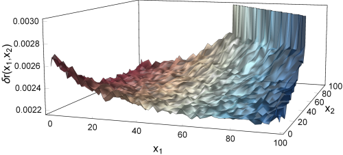
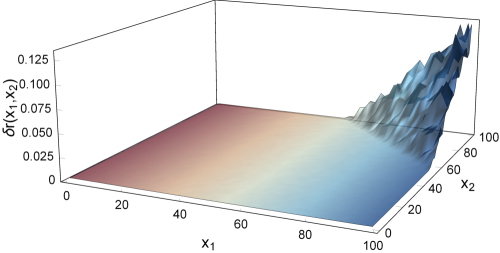
Figure 3: Relative error $\delta r(x_{1},x_{2})$ with $x_{1}=x_{2}=\{0,1,2,\cdots 99\}$. The cluster contains three nodes. One node contains 2 K80m, one contains 4 K40m and another contains one V100. $x_{1}$ and $x_{2}$ expand a parameter grid, and at each grid value we plot the relative error of the integration. In the upper panel we have clipped the $\delta r$ axis such that the variations for low error regions can be seen clearly, while in the lower panel, we have plotted the full range of $\delta r$.

3.3 Functional integration for relativistic Boltzmann equation

A straight forward application of ZMCintegral-v5 is the solving of the relativistic Boltzman Equation for Quark Gluon plamsa[19]. There, we have seven coupled first order differential equations with an integration of 5 dimensions

$$\frac{\partial\widetilde{f}_{\mathbf{p}}^{a}(x)}{\partial t}+\frac{\mathbf{p}}{E_{\mathbf{p}}^{a}(x)}\cdot\nabla_{x}\widetilde{f}_{\mathbf{p}}^{a}(x)$$

$$-\nabla_{x}\left[E_{\mathbf{p}}^{a}(x)\right]\cdot\nabla_{\mathbf{p}}\widetilde{f}_{\mathbf{p}}^{a}(x) = C_{a}(\mathbf{x},\mathbf{p}),$$ (6)

where $\widetilde{f}_{\mathbf{p}}^{a}(x)$, the color and spin averaged distribution function for particle $a$ ($a$ denotes u,d,s,$\bar{\text{u}}$,$\bar{\text{d}}$,$\bar{\text{s}}$ and gluon), is a function of space-time $x^{\mu}=(t,\mathbf{x})$ and momentum $p^{\mu}=(E_{\mathbf{p}},\mathbf{p})$, $C_{a}(\mathbf{x},\mathbf{p})$ is the collision term (5 dimensional integration) for quarks or gluon, $E_{\mathbf{p}}(\mathbf{x})=\sqrt{\mathbf{p}^{2}+m_{a}^{2}(\mathbf{x})}$. The complexity of this equation lies in the collision term $C_{a}(\mathbf{x},\mathbf{p})$ which has a large parameter grid.

For Eq. (6), the parameter grid is $\widetilde{f}_{\mathbf{p}}^{a}(\mathbf{x})$ where $\mathbf{p}=[p_{x},p_{y},p_{z}]$, $\mathbf{x}=[x,y,z]$ and $a$ being u,d,s,$\bar{\text{u}}$,$\bar{\text{d}}$,$\bar{\text{s}}$ and gluon. This is a large parameter grid with $[n_{p_{x}},n_{p_{y}},n_{p_{z}},n_{x},n_{y},n_{z}]=[30,30,30,10,10,10]$. Threfore we have $30^{3}\times 10^{3}\times 7\sim 2\times 10^{8}$ grid points to scan. When evaluate $C_{a}(\mathbf{x},\mathbf{p})$, which is a 5 dimensional integration, since $\mathbf{x}$ and $\mathbf{p}$ are parameters, we need to evaluate $2\times 10^{8}$ $C_{a}$. For this specific task, our previous versions perform poorly since users have to provide the parameter grid in CPU, and evaluate each integration in GPU one by one. The newest version, which returns the entire parameter grid from GPU with each element being the integrated values, saves much of the communication time between Host (CPU) and Device (GPU). Thus it is more suitable for large parameter scan and relatively lower dimensional integrations.

4 Conclusion and Discussion

To meet the requirement of integration with large parameter grids, we have added a new functionality to ZMCintegral-5 which is able to give the integration results at each grid point on multi-GPUs. The code supports user defined functions and is easy to use in the Python language. To ensure the calculation speed, we only adopt the direct Monte Carlo method to evaluate integrations. For the parameter scan functionality, we suggest a number of sample points not exceed $10^{6}$ (for parameter grid size ~ $10^{8}$) for one Tesla V100. However, for users with large GPU clusters, this number can be set higher. The time consumption for data transfer from host to device and between different nodes is negligible compared with the GPU evaluation time. Therefore, users only need to consider the number of sample points, which determines the accuracy and calculation time of the integration task.

References

- [1] H.-Z. Wu, J.-J. Zhang, L.-G. Pang, Q. Wang, ZMCintegral: A package for multi-dimensional monte carlo integration on multi-GPUs, Computer Physics Communications (2019) 106962doi:10.1016/j.cpc.2019.106962.
- [2] C. Shi, Y. long Wang, Y. Jiang, Z. fang Cui, H.-S. Zong, Locate QCD critical end point in a continuum model study, Journal of High Energy Physics 2014 (7). doi:10.1007/jhep07(2014)014.
- [3] C. Shi, Y.-L. Du, S.-S. Xu, X.-J. Liu, H.-S. Zong, Continuum study of the QCD phase diagram through an OPE-modified gluon propagator, Physical Review D 93 (3). doi:10.1103/physrevd.93.036006.
- [4] B.-Y. Cui, Y.-Y. Fan, F.-H. Liu, W.-F. Wang, Quasi-two-body decays in the perturbative qcd approacharXiv:http://arxiv.org/abs/1906.09387v2, doi:10.1103/PhysRevD.100.014017.
- [5] A. Kurkela, A. Mazeliauskas, Chemical equilibration in weakly coupled QCD, Physical Review D 99 (5). doi:10.1103/physrevd.99.054018.
- [6] S. R. De Groot, Relativistic Kinetic Theory. Principles and Applications, 1980.
- [7] Z. Xu, C. Greiner, Thermalization of gluons in ultrarelativistic heavy ion collisions by including three-body interactions in a parton cascade, Physical Review C 71 (6). doi:10.1103/physrevc.71.064901.
- [8] J. jie Zhang, R. hong Fang, Q. Wang, X.-N. Wang, A microscopic description for polarization in particle scatteringsarXiv:http://arxiv.org/abs/1904.09152v1.
- [9] J. Back, T. Gershon, P. Harrison, T. Latham, D. O’Hanlon, W. Qian, P. del Amo Sanchez, D. Craik, J. Ilic, J. M. O. Goicochea, E. Puccio, R. S. Coutinho, M. Whitehead, Laura++mathplus: A dalitz plot fitter, Computer Physics Communications 231 (2018) 198–242. doi:10.1016/j.cpc.2018.04.017.
- [10] F. James, MINUIT Function Minimization and Error Analysis: Reference Manual Version 94.1.
-
[11]
G. P. Lepage,
A
new algorithm for adaptive multidimensional integration, Journal of
Computational Physics 27 (2) (1978) 192 – 203.
doi:https://doi.org/10.1016/0021-9991(78)90004-9.
URL http://www.sciencedirect.com/science/article/pii/0021999178900049 -
[12]
S. Jadach,
Foam:
A general-purpose cellular monte carlo event generator, Computer Physics
Communications 152 (1) (2003) 55 – 100.
doi:https://doi.org/10.1016/S0010-4655(02)00755-5.
URL http://www.sciencedirect.com/science/article/pii/S0010465502007555 - [13] I. Buck, T. Purcell, A Toolkit for Computation on GPUs, 2004.
- [14] K. E. Niemeyer, C.-J. Sung, GPU-based parallel integration of large numbers of independent ODE systems, in: Numerical Computations with GPUs, Springer International Publishing, 2014, pp. 159–182.
- [15] S. Kwan Lam, A. Pitrou, S. Seibert, Numba: a llvm-based python jit compiler, 2015, pp. 1–6. doi:10.1145/2833157.2833162.
-
[16]
P. Moritz, R. Nishihara, S. Wang, A. Tumanov, R. Liaw, E. Liang, M. Elibol,
Z. Yang, W. Paul, M. I. Jordan, I. Stoica,
Ray: A
distributed framework for emerging AI applications, in: 13th USENIX
Symposium on Operating Systems Design and Implementation (OSDI 18),
USENIX Association, Carlsbad, CA, 2018, pp. 561–577.
URL https://www.usenix.org/conference/osdi18/presentation/moritz - [17] A. B. Owen, Monte Carlo theory, methods and examples, 2013.
- [18] Location of zmcintegral package, https://github.com/Letianwu/ZMCintegral.git.
- [19] to be published.
-
[20]
R. E. Bellman,
Dynamic
Programming, PRINCETON UNIV PR, 1957.
URL https://www.ebook.de/de/product/34448612/richard_e_bellman_dynamic_programming.html -
[21]
R. Bellman,
Dynamic
Programming, Dover Publications Inc., 2003.
URL https://www.ebook.de/de/product/3396699/richard_bellman_dynamic_programming.html - [22] J.-W. Chen, Y.-F. Liu, Y.-K. Song, Q. Wang, Shear and bulk viscosities of a weakly coupled quark gluon plasma with finite chemical potential and temperature: Leading-log results, Physical Review D 87 (3). doi:10.1103/physrevd.87.036002.
-
[23]
M. E. Peskin, D. V. Schroeder,
An Introduction to
quantum field theory, Addison-Wesley, Reading, USA, 1995.
URL http://www.slac.stanford.edu/~mpeskin/QFT.html -
[24]
J. Kanzaki, Monte carlo
integration on gpu, The European Physical Journal C 71 (2) (2011) 1559.
doi:10.1140/epjc/s10052-011-1559-8.
URL https://doi.org/10.1140/epjc/s10052-011-1559-8 -
[25]
S. Kawabata,
A
new version of the multi-dimensional integration and event generation package
bases/spring, Computer Physics Communications 88 (2) (1995) 309 – 326.
doi:https://doi.org/10.1016/0010-4655(95)00028-E.
URL http://www.sciencedirect.com/science/article/pii/001046559500028E -
[26]
M. Abadi, P. Barham, J. Chen, Z. Chen, A. Davis, J. Dean, M. Devin,
S. Ghemawat, G. Irving, M. Isard, M. Kudlur, J. Levenberg, R. Monga,
S. Moore, D. G. Murray, B. Steiner, P. Tucker, V. Vasudevan, P. Warden,
M. Wicke, Y. Yu, X. Zheng,
Tensorflow:
A system for large-scale machine learning, in: 12th USENIX Symposium on
Operating Systems Design and Implementation (OSDI 16), USENIX
Association, Savannah, GA, 2016, pp. 265–283.
URL https://www.usenix.org/conference/osdi16/technical-sessions/presentation/abadi - [27] I. Deák, Uniform random number generators for parallel computers, Parallel Computing 15 (1990) 155–164. doi:10.1016/0167-8191(90)90039-C.
- [28] J. Bendavid, Efficient monte carlo integration using boosted decision trees and generative deep neural networks.
- [29] M. Abadi, A. Agarwal, P. Barham, E. Brevdo, Z. Chen, C. Citro, G. Corrado, A. Davis, J. Dean, M. Devin, S. Ghemawat, I. Goodfellow, A. Harp, G. Irving, M. Isard, Y. Jia, L. Kaiser, M. Kudlur, J. Levenberg, X. Zheng, Tensorflow : Large-scale machine learning on heterogeneous distributed systems (01 2015).
-
[30]
T. Ohl,
Vegas
revisited: Adaptive monte carlo integration beyond factorization, Computer
Physics Communications 120 (1) (1999) 13 – 19.
doi:https://doi.org/10.1016/S0010-4655(99)00209-X.
URL http://www.sciencedirect.com/science/article/pii/S001046559900209X -
[31]
R. Kreckel,
Parallelization
of adaptive mc integrators, Computer Physics Communications 106 (3) (1997)
258 – 266.
doi:https://doi.org/10.1016/S0010-4655(97)00099-4.
URL http://www.sciencedirect.com/science/article/pii/S0010465597000994 - [32] Tensorflow eager mode, https://www.tensorflow.org/guide/eager.
- [33] Vegas tutorial, https://www.vegas.readthedocs.io/en/latest/tutorial.html.
- [34] P. Jian-wei, The quantum computing: Present and future, MIT China Submit (2018).
- [35] J. Nickolls, W. J. Dally, The gpu computing era, IEEE Micro 30 (2) (2010) 56–69. doi:10.1109/MM.2010.41.